INSTITUTE OF PHYSICS PUBLISHING PHYSICS IN MEDICINE AND BIOLOGY

Phys. Med. Biol. 51 (2006) 3189–3210 doi:10.1088/0031-9155/51/12/013

A shift-invariant filtered backprojection (FBP)cone-beam reconstruction algorithm for the sourcetrajectory of two concentric circles using an equalweighting scheme

Tingliang Zhuang1, Brian E Nett1, Shuai Leng1 and Guang-Hong Chen1,2

1 Department of Medical Physics, University of Wisconsin-Madison, Madison, WI 53704, USA2 Department of Radiology, University of Wisconsin-Madison, Madison, WI 53792, USA

E-mail: gchen7@wisc.edu

Received 2 December 2005, in final form 21 April 2006Published 6 June 2006Online at stacks.iop.org/PMB/51/3189

AbstractIn this paper, a shift-invariant filtered backprojection cone-beam imagereconstruction algorithm is derived, based upon Katsevich’s general inversionscheme, and validated for the source trajectory of two concentric circles. Thesource trajectory is complete according to Tuy’s data sufficiency condition andis used as the basis for an exact image reconstruction algorithm. The algorithmproceeds according to the following steps. First, differentiate the cone-beamprojection data with respect to the detector coordinates and with respect tothe source trajectory parameter. The data are then separately filtered alongthree different orientations in the detector plane with a shift-invariant Hilbertkernel. Eight different filtration groups are obtained via linear combinationsof weighted filtered data. Voxel-based backprojection is then carried outfrom eight sets of view angles, where separate filtered data are backprojectedfrom each set according to the backprojection sets’ associated filtration group.The algorithm is first derived for a scanning configuration consisting of twoconcentric and orthogonal circles. By performing an affine transformationon the image object, the developed image reconstruction algorithm has beengeneralized to the case where the two concentric circles are not orthogonal.Numerical simulations are presented to validate the reconstruction algorithmand demonstrate the dose advantage of the equal weighting scheme.

(Some figures in this article are in colour only in the electronic version)

0031-9155/06/123189+22$30.00 © 2006 IOP Publishing Ltd Printed in the UK 3189

3190 T Zhuang et al

1. Introduction

The recent developments in large-area flat-panel detectors have encouraged increasedinvestigations in cone-beam computed tomography (CT). One example of the use of suchdetectors in medical imaging is in the case of interventional C-arm systems. These C-armsystems enable flexible data acquisition due to the presence of multiple independent motioncontrol motors. This flexible data acquisition provides the opportunity for mathematicallyexact reconstruction of a volume of interest (VOI). The desire for mathematically exactreconstruction is to eliminate the cone-beam artefacts present when images are reconstructedfrom data collected from a single circle. Examples of such data acquisition modes include theCC-geometry (which consists of two concentric arcs) proposed at the University of Wisconsinin Madison (Chen et al 2003) and the saddle trajectories proposed by other investigators(Pack et al 2004). The CC-geometry utilizes a source trajectory consisting of subsets of twoconcentric circles with equal radius and thus the trajectories which may be formed using thisgeometry include circle plus circle, circle plus arc, circle plus multiple arcs and arc plus arc.The scanning geometry of two concentric complete circles (Tuy 1983) can be considered as aspecial limit of the proposed CC-geometry when the angular ranges for two arcs are 2π . Onemay envision that in future small animal imaging or industrial CT applications one may utilizethis source trajectory. The two concentric circles with equal radius generate a complete cone-beam projection data set in the sense of the Tuy data sufficiency condition (Tuy 1983). Thiscompleteness condition distinguishes the two-concentric-circle case from the trajectories of asingle arc or a single circular source trajectory. Note that the two-orthogonal-circle trajectoryis a special case of the two-concentric-circle trajectory.

In this paper, we develop a shift-invariant and mathematically exact filtered backprojection(FBP) image reconstruction algorithm for two concentric circles. These two concentriccircles may be either orthogonal or non-orthogonal. The basic method used to developa shift-invariant FBP image reconstruction algorithm for a general source trajectory hasbeen outlined by Katsevich (2003) and by one of the present authors (Chen 2003). Theessence of this method for generating exact reconstruction algorithms is to analyse thestructure factor of the scanning geometry. The structure factor dictates the correspondingstructure of the backprojection segments as discussed below. It is important to note thatthe structure factor is highly dependent upon the choice of the weighting function forredundantly measured projection data. Theoretically, an equal weighting is optimal withrespect to the noise properties of the reconstruction algorithm (Parker et al 1981). This equalweighting scheme has previously been utilized to develop a cone-beam image reconstructionalgorithm from a single arc scanning trajectory (Zhuang et al 2004b) using the general shift-invariant FBP cone-beam image reconstruction framework (Katsevich 2003, Chen 2003).In the current work, the same equal weighting scheme was used in the calculation of thestructure factor. Using an equal weighting scheme, as argued by Katsevich (2003), themagnitude of the structure factor is either 1

2 or 14 in a scanning configuration of two concentric

and orthogonal complete circles. However, the calculation of the structure factor was notexplicitly carried out by Katsevich (2003). This structure factor is necessary in order toobtain a numerically implementable reconstruction algorithm. In this work, the explicitcalculation of the structure factor is carried out to derive an explicit image reconstructionalgorithm for the scanning configuration of two concentric and orthogonal circles. Afterintroducing an affine transformation, the derived shift-invariant image reconstructionalgorithm for a source trajectory consisting of two concentric and orthogonal circles hasbeen generalized to the source trajectories consisting of two concentric non-orthogonalcircles.

A shift-invariant FBP cone-beam reconstruction algorithm 3191

x

β

y(t)

x

v

u w

z

t

y

o

S

D

Figure 1. The geometric parameters used in this paper are provided above. The origin of theworld coordinate system (o) is shown and a Cartesian coordinate system is established. The sourcetrajectory is parameterized by the angle t and a given source position is thus referenced as �y(t).The vector β originates at �y(t) and points towards a given image point.

An overview of the properties of the derived reconstruction algorithm is given below.This algorithm utilizes projection data from every source position in order to reconstructeach image point. In order to facilitate the numerical implementation, the differentiation ofthe cone-beam projection data with respect to the source parameter, for a fixed projectiondirection, has been expressed using the detector coordinates and the direct partial derivativeof the cone-beam projection data with respect to the source parameter. After the data havebeen differentiated, they are separately filtered along three different orientations using a 1Dshift-invariant Hilbert kernel. This yields three sets of filtered data. Eight filtration groups areobtained by linear combinations of the weighted filtered data. Voxel-specific backprojectionis carried out from the eight sets of view angles, where separate filtered data are backprojectedfrom each set according to the backprojection sets’ associated filtration group. In order tovalidate the developed algorithm, mathematically generated cone-beam projection data, withand without Poisson noise, from the standard Shepp–Logan and Defrise phantoms were used inthe numerical simulations. There has been significant research directed towards reconstructingan image function from cone-beam projections acquired from circle-based trajectories. Thenovel features of this algorithm in comparison with the previously published analytic methodsfor such trajectories will be covered in the discussion section.

2. Cone-beam reconstruction algorithm for a complete source trajectory

2.1. The data acquisition geometry

In this paper, a third-generation cone-beam source–detector configuration is used. Thecoordinate system is shown in figure 1. Letter ‘o’ labels the isocentre of rotation. Thecoordinate system x–y–z located at ‘o’ is denoted as the world system. The detector plane isperpendicular to the iso-ray originating from the source point S. The distance along the iso-ray

3192 T Zhuang et al

between the source and the detector is D. In the world system, the point �x of the object iswritten as �x = (x, y, z). The density of a 3D object to be reconstructed is denoted as f (�x).The cone-beam projection of the object from the source point �y(t) is written as

g(r, t) =∫ ∞

0dsf [ �y(t) + sr], (1)

where r is a unit vector originating from the source point �y(t).

2.2. Review of cone-beam FBP reconstruction algorithm for a complete source trajectory

In this subsection, we will briefly review the main results of the cone-beam FBP reconstructionframework (Katsevich 2003, Chen 2003) for a general source trajectory fulfilling Tuy’s datasufficiency condition (Tuy 1983).

The unit vector originating from source position �y(t) and passing through a point �x of theobject will be denoted as β:

β = �x − �y(t)

| �x − �y(t)| = (cos β sin α, sin β sin α, cos α), (2)

where α and β are the longitudinal and azimuthal angles which are functions of the imagepoint �x and the source point �y(t). A plane containing the unit vector β is now introducedwhich can be characterized by its normal vector. After properly selecting a local coordinatesystem, the normal vector of this plane may be locally parameterized by an angle φ (Chen2003). In the world system, this normal vector can be represented by

kφ = ζ cos φ + β × ζ sin φ, (3)

where the unit vector ζ can be chosen to be ζ = (−sin β, cos β, 0). Throughout this paper,the plane containing β and having normal vector kφ will be denoted as �( �x, t;φ). Any unitvector r which originates from the source position S and lies within the plane �( �x, t;φ) maybe represented as

r(γ, φ) = β cos γ + β × kφ sin γ, γ ∈ [−π, π ]. (4)

The Katsevich-type cone-beam reconstruction formula (Chen 2003) is given by

f ( �x) = − 1

4π2

∑m

∫dt

cm( �x, t)

| �x − �y(t)|∫ π

−π

dγ1

sin γ

∂

∂qg[r(γ, φm), �y(q)]|q=t , (5)

where φm ∈ [0, π). The function cm( �x, t) termed as the structure factor is determined asfollows:

cm( �x, t) = limε→0+

sgn[kφ · �y ′(t)]w[ �x, kφ; t]|φ=φm+εφ=φm−ε, (6)

where either the function sgn[kφ · �y ′(t)] or the weighting function w[ �x, kφ; t] as a function ofφ will be discontinuous at the angle φm. The weighting function w[ �x, kφ; t] is introduced totake into account the data redundancy when a plane containing the image point intersects thesource trajectory more than once.

Obviously, the angle φm is a function of the image point �x and the source point �y(t),namely φm = φm( �x, t)). In this paper, the angle φm and the plane �( �x, t;φ = φm( �x, t))

will be referred to as the critical angle and the critical plane, respectively. The intersectionsbetween the critical planes �( �x, t;φm( �x, t)) and the detector plane provide the directions forthe filtering operation and thus will be referred to as the filtering lines.

In summary, to reconstruct an image point �x using a Katsevich-type cone-beam algorithm,the following steps may be utilized:

A shift-invariant FBP cone-beam reconstruction algorithm 3193

z

x

y

z’

x’

y’

(a) (b)

Figure 2. (a) The source trajectory shown in the original coordinate system where the horizontalcircle lies in the x–y plane and the vertical circle lies in the y–z plane. (b) The source trajectoryshown in the new coordinate system after rotation where the horizontal circle lies in the y′–z′ planeand the vertical circle lies in the x′–y′ plane.

• Step 1: extract the measured projection data from the critical planes �( �x, t;φm( �x, t)) foreach source point �y(t).

• Step 2: differentiate the projection data with respect to the source parameter t.• Step 3: perform a 1D filtering operation using a modified Hilbert filtering kernel

1sin γ

along the filtering lines determined by the intersection between the critical planes�( �x, t;φm( �x, t)) and the detector.

• Step 4: sum the contributions from the critical planes �( �x, t;φm( �x, t)) using the weightgiven by the structure factors cm( �x, t).

• Step 5: perform a distance-weighted backprojection.

It is important to point out that the process described above involves a shift-invariantfiltering operation; thus, in implementation the filtration step may be conducted only oncein order to reconstruct the entire volume. From the above steps, we see that it is importantto determine the critical plane and the associated structure factor which is highly dependentupon the weighting function. As discussed by Chen (2003), to obtain the above reconstructionformula, a necessary condition on the weighting function has to be imposed:

∂

∂φw[ �x, kφ; t] = 0. (7)

A natural choice of a weighting function which satisfies the above condition is

w[ �x, kφ; t] = 1

n[ �x, kφ; t], (8)

where n[ �x, kφ; t] is the number of intersecting points between the plane �( �x, t;φ) and thesource trajectory. The equal weighting scheme is desirable as it yields optimal noise propertiesin the resulting reconstruction algorithm (Parker et al 1981). In this paper, the equal weightingscheme will be used to derive a cone-beam reconstruction formula for the source trajectoryconsisting of two orthogonal circles.

3. Cone-beam reconstruction algorithm for the two-orthogonal-circle source trajectory

As shown in figure 2(a), a two-orthogonal-circle source trajectory with radius R can beparameterized by t as follows:

3194 T Zhuang et al

�yh(t) = R(cos t, sin t, 0), t ∈ [0, 2π), (9)

�yv(t) = R(0,−sin t, cos t), t ∈ [2π, 4π). (10)

Here, the subscripts ‘h’ and ‘v’ denote the horizontal and vertical circles, respectively. Sincethe backprojection step is linear, the reconstruction formula for this source trajectory maybe written as the summation of backprojections from the horizontal and vertical circles,respectively. Namely,

f ( �x) = fh( �x) + f v( �x). (11)

In order to obtain the explicit expressions for fh( �x) and f v( �x), the key is to calculatethe structure factor cm( �x, t) for t ∈ [0, 4π). In the following, we show that the expressionsof cm( �x, t) for t ∈ [2π, 4π) can be obtained from those for t ∈ [0, 2π) due to a symmetryproperty of the two-orthogonal-circle scanning geometry. As shown in figure 2(b), if thecoordinate is transformed using

{x, y, z} → {x ′ = z, y ′ = −y, z′ = x}, (12)

then the following relationship exists between the horizontal and vertical scanning paths:

�yh(t) ↔ �yv(t). (13)

Therefore, the vertical circle (lies in the y–z plane) in the original coordinate system will be a‘horizontal’ circle (lies in the x ′-y ′ plane) in the coordinate system after transformation. Sincethe structure factor only depends on the geometric configuration of the source trajectory, weconclude that

cm( �x ′, t) for t ∈ [2π, 4π) = cm( �x, t) for t ∈ [0, 2π). (14)

Thus, the formula used to calculate the contributions from the horizontal circle (fh( �x)) canalso be used to calculate the contributions from the vertical circle (f v( �x)) with two changes:(1) the reconstruction point �x = (x, y, z) should be replaced by the point �x ′ = (z,−y, x);(2) the cone-beam projection data acquired from the horizontal circle should be replaced bythose from the vertical circle. Namely,

f v( �x) = fv( �x ′). (15)

In summary, the reconstruction formula (11) may be written as

f ( �x) = fh( �x) + fv( �x ′). (16)

In the following section, we will first present the result for the source moving along thehorizontal circle.

3.1. The image reconstruction structure for the horizontal circular trajectory

As discussed above, due to the symmetry of the acquisition geometry, a simple transformationis sufficient to obtain the part of reconstruction formula for the source residing in the verticalcircle when one has the horizontal reconstruction formula. In this section, we will present thestructure of the reconstruction formula for the source located in the horizontal circle.

For the third-generation flat-panel-detector data acquisition geometry, it is convenient todefine the following rotating coordinate system for the horizontal source trajectory:

w = (−cos t,−sin t, 0), u = (sin t,−cos t, 0), v = (0, 0, 1).

A shift-invariant FBP cone-beam reconstruction algorithm 3195

The detector Cartesian coordinates u, v which are measured in the detector plane alongdirections u, v are given below (Noo et al 2003):

u = Dr · u

r · w, v = D

r · v

r · w. (17)

Equation (5) can be rewritten using detector coordinate as follows (Zhuang et al 2004b):

f ( �x) = − 1

4π2

∑m

∫dt

cm( �x, t)

L( �x, t)Qm[uβ( �x, t), vβ( �x, t), t], (18)

whereL( �x, t) = R − x cos t − y sin t,

Qm[u, v, t] =∫ +∞

−∞

∫ +∞

−∞du dv δ[v − v − κm(u − u)]hH(u − u)g(u, v, t),

g(u, v, t) = D√D2 + u2 + v2

(D2 + u2

D

∂

∂u+

uv

D

∂

∂v− ∂

∂t

)g(u, v, t)

(19)

and

uβ( �x, t) = Dx sin t − y cos t

L( �x, t), vβ( �x, t) = D

z

L( �x, t); (20)

hH(x) = 1x

is the kernel of Hilbert transform and κm is the slope of the filtering line wherethe plane �( �x, t;φm) intersects the detector plane. The calculation of the structure factor,cm( �x, t) for t ∈ [0, 2π), will be discussed in the next subsection.

3.2. Structure factor

The structure factor is given by the amplitude of the discontinuity of the product of theweighting function w( �x, kφ; t) and the function sgn[kφ · �y ′(t)] for t ∈ [0, 2π). In the following,we will separately study the dependence on the angle φ of the weighting function w( �x, kφ; t)

defined in equation (8) and the function sgn[kφ · �y ′(t)].

3.2.1. Analysis of the weighting function. The purpose of this section is to determinethe number of intersection points between the plane �( �x, t;φ), t ∈ [0, 2π) and the twoorthogonal circles. Once the number of intersection points is calculated, the weightingfunction is expressed as simply the inverse of the number of intersection points.

Any point �x0 in the plane �( �x, t;φ) can be described by the following equation:

kφ · ( �x0 − �x) = 0. (21)

Since this plane also passes through the source point �yh(t), the above equation can also bewritten as

kφ · [ �x0 − �yh(t)] = 0. (22)

For fixed values of �x and t ∈ [0, 2π), by setting �x0 = �yh(t′) or �x0 = �yv(t

′) and determiningthe number of values of t ′ which satisfy the above equation, we can obtain the number ofintersection points between the plane �( �x, t;φ) and the horizontal as well as the verticalcircle.

First, let us consider the number of intersection points between the plane �( �x, t;φ) andthe horizontal circle by setting �x0 = �yh(t

′) in (22). Almost every plane (�( �x, t;φ) with adifferent value of φ) will intersect with the horizontal circle twice. The exception is the plane�( �x, t;φ = φtan( �x, t)), where

cot φtan( �x, t) = cos α tan(β − t). (23)

3196 T Zhuang et al

In order to clarify the meaning of this condition, we consider the following two situations forthe intersections between the plane �( �x, t;φ = φtan( �x, t)) and the horizontal source. Theplane �( �x in = (x, y, 0), t;φ = φtan( �x in, t)) intersects the horizontal circle infinitely manytimes and the plane �( �xoff = (x, y, z �= 0), t;φ = φtan( �xoff, t)) is tangential to the horizontalcircle (intersecting once). In any case, the weighting function w[ �x, kφ; t] will be discontinuousat the angle φ = φtan( �x, t) due to the change of the number of the intersection points betweenthe �( �x, t;φ) plane and the horizontal circle.

Second, let us consider the number of intersection points between the plane �( �x, t;φ)

and the vertical circle by setting �x0 = �yv(t′) in (22). After substituting the expression of kφ

(equation (3)) into equation (22), we obtain

l1(φ;α, β, t) cos t ′ + l2(φ;α, β, t) sin t ′ = l3(φ;α, β, t)

=√

l21(φ;α, β, t) + l2

2(φ;α, β, t) cos(t ′ + ξ), (24)

wherel1(φ;α, β, t) = sin α sin φ,

l2(φ;α, β, t) = cos α sin β sin φ − cos β cos φ,

l3(φ;α, β, t) = −sin(β − t) cos φ − cos α cos(β − t) sin φ,

ξ = tan−1

[l2(φ;α, β, t)

l1(φ;α, β, t)

].

(25)

This equation can be simplified as

cos(t ′ + ξ) = l3(φ;α, β, t)√l21(φ;α, β, t) + l2

2(φ;α, β, t)

. (26)

The number of solutions for t ′ of (26) is equal to the number of intersection points betweenthe vertical source trajectory and the �( �x, t;φ) plane. If the magnitude of the right-hand side(rhs) of equation (26) is greater than unity there are no solutions to the equation, otherwisethere are either one or two solutions to equation (26). In order to find the number of solutionsfor t ′ in equation (26), we introduce the following function p( �x, t;φ):

p( �x, t;φ) = l21(φ;α, β, t) + l2

2(φ;α, β, t) − l23(φ;α, β, t)

= [p1(α, β, t) cot2 φ + p2(α, β, t) cot φ + p3(α, β, t)] sin2 φ, (27)

where

p1(α, β, t) = cos2 β − sin2(β − t),

p2(α, β, t) = −2 cos α sin(2β − t) cos t,

p3(α, β, t) = sin2 α − [cos2 β − sin2(β − t)] cos2 α.

Therefore, for a given image point �x and a source point �yh(t), t ∈ [0, 2π) on the horizontalcircle, the number of intersection points between the plane �( �x, t, ;φ0) (a plane parameterizedby angle φ0 that passes through the points �x and �yh(t)) and the vertical circle will be determinedby investigating the corresponding value p( �x, t;φ0):

• If p( �x, t;φ0) > 0, then there will be two solutions of equation (26). Therefore, thereexist two intersections between �( �x, t;φ0) and the vertical circle.

• If p( �x, t;φ0) = 0, then there will be one solution of equation (26). Therefore, there existsone intersection between �( �x, t;φ0) and the vertical circle.

• If p( �x, t;φ0) < 0, then there is no solution of equation (26). Therefore, there is nointersection between �( �x, t;φ0) and the vertical circle.

A shift-invariant FBP cone-beam reconstruction algorithm 3197

Therefore, using the plot of φ–p( �x, t;φ), the discontinuity of the weighting functionw[ �x, kφ; t] due to the change in the number of intersections between the plane �( �x, t;φ) withthe vertical circle can be obtained:

• Case 1: the plot of p( �x, t;φ) with respect to the angle φ intersects with the φ-axis atφn1( �x, t) and φn2( �x, t). The discontinuity in the weighting function w[ �x, kφ; t] will occurat φ = φn1( �x, t), φn2( �x, t). Note that these two critical angles may be equal to each other.

• Case 2: the plot of p( �x, t;φ) with respect to the angle φ does not intersect with the φ-axis.There is no discontinuity in the weighting function.

In summary, the discontinuities in the weighting function w[ �x, kφ; t] will occur atφ = φtan( �x, t), φn1( �x, t), φn2( �x, t), due to the change in the number of intersection pointsbetween the �( �x, t;φ) plane and either the horizontal circle or the vertical one.

3.2.2. Analysis of the sgn function. Let us consider sgn[kφ · �y ′h(t)]. The argument of this

function is calculated to be

kφ · �y ′h(t) = D

2

√cos2(β − t) + cos2 α sin2(β − t) sin(φ − φh( �x, t)). (28)

Then we have

sgn[kφ · �y ′h(t)] =

{−1, if φ ∈ [0, φh( �x, t)),

1, if φ ∈ (φh( �x, t), π ].(29)

3.2.3. Explicit form of the structure factor. Using the results in the preceding subsections,we obtain the structure factor for t ∈ [0, 2π):

ctan( �x, t) = 12 , for t ∈ T1( �x) ∪ T21( �x) ∪ T22( �x) ∪ T3( �x) = [0, 2π), (30)

cn1( �x, t) ={ 1

4 , if t ∈ T1( �x) ∪ T21( �x),

−14 , if t ∈ T22( �x),

(31)

cn2( �x, t) ={ 1

4 , if t ∈ T1( �x) ∪ T22( �x),

−14 , if t ∈ T21( �x),

(32)

where

T1( �x) = {t |p1(α, β, t) < 0, (α, β, t) > 0},T21( �x) = {t |p1(α, β, t) > 0, (α, β, t) > 0} ∩ {

t |φtan( �x, t) < φn1( �x, t)},

T22( �x) = {t |p1(α, β, t) > 0, (α, β, t) > 0} ∩ {t |φtan( �x, t) > φn2( �x, t)

},

T3( �x) = {t | (α, β, t) < 0},with

(α, β, t) = p22(α, β, t) − 4p1(α, β, t)p3(α, β, t). (33)

The explicit expressions of these sets are given in the appendix.

3.3. Final formula

Based on the symmetry of the data acquisition geometry, utilizing the coordinatetransformation introduced in equation (12), we obtain the following reconstruction formula:

f ( �x) = fh( �x) + fv( �x ′), (34)

3198 T Zhuang et al

where

−4π2fs( �x) =∑A

∫TA( �x)

dt1

L( �x, t)Qs

A[uβ( �x, t), vβ( �x, t), t], (35)

with QsA(u, v, t), A = 1, 21, 22, 3, s = h, v, given by

Qs1(u, v, t) = 1

2qs0(u, v, t) + 1

4qs1(u, v, t) + 1

4qs2(u, v, t),

Qs21(u, v, t) = 1

2qs0(u, v, t) + 1

4qs1(u, v, t) − 1

4qs2(u, v, t),

Qs22(u, v, t) = 1

2qs0(u, v, t) − 1

4qs1(u, v, t) + 1

4qs2(u, v, t),

Qs3(u, v, t) = 1

2qs0(u, v, t),

(36)

where

qs0(u, v, t) =

∫duhH(u − u)gs[u, v, t],

qs1(u, v, t) =

∫duhH(u − u)gs[u, v1(u, v, t), t],

qs2(u, v, t) =

∫duhH(u − u)gs[u, v2(u, v, t), t]

(37)

and

vm(u, v, t) = v + κm

(u

D,

v

D, t

)(u − u),

κm(y1, y2, t) = −y1y2 cos2 t − 12y2 sin(2t)(

1 − y21

)cos2 t − y1 sin(2t)

+(−1)m−1

√(y2

1 + y22 − 1

)cos2 t + y1 sin(2t)(

1 − y21

)cos2 t − y1 sin(2t)

.

Here the index m may take value 1 or 2. Before passing, we would like to point out that thereare eight filtration groups since index s may take either ‘h’ or ‘v’ in equation (36).

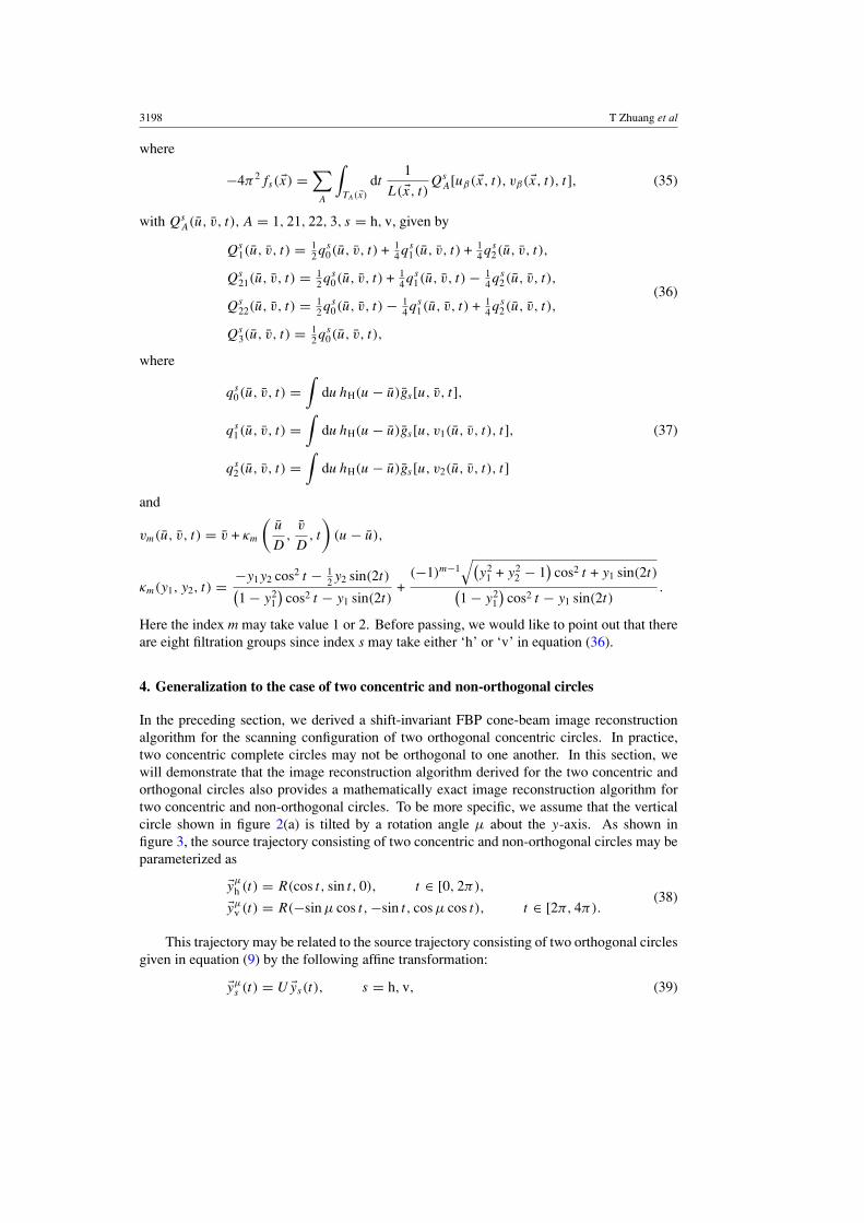
4. Generalization to the case of two concentric and non-orthogonal circles

In the preceding section, we derived a shift-invariant FBP cone-beam image reconstructionalgorithm for the scanning configuration of two orthogonal concentric circles. In practice,two concentric complete circles may not be orthogonal to one another. In this section, wewill demonstrate that the image reconstruction algorithm derived for the two concentric andorthogonal circles also provides a mathematically exact image reconstruction algorithm fortwo concentric and non-orthogonal circles. To be more specific, we assume that the verticalcircle shown in figure 2(a) is tilted by a rotation angle µ about the y-axis. As shown infigure 3, the source trajectory consisting of two concentric and non-orthogonal circles may beparameterized as

�yµ

h (t) = R(cos t, sin t, 0), t ∈ [0, 2π),

�yµv (t) = R(−sin µ cos t,−sin t, cos µ cos t), t ∈ [2π, 4π).

(38)

This trajectory may be related to the source trajectory consisting of two orthogonal circlesgiven in equation (9) by the following affine transformation:

�yµs (t) = U �ys(t), s = h, v, (39)

A shift-invariant FBP cone-beam reconstruction algorithm 3199

x

y

z

µ

o

Figure 3. Demonstration of the source trajectory consisting of two concentric non-orthogonalcircles. The vertical circle is tilted by an angle µ about the y-axis clockwise.

U =1 0 −sin µ

0 1 00 0 cos µ

, U−1 =

1 0 tan µ

0 1 00 0 1

cos µ

. (40)

As demonstrated by Noo et al (2004), exact reconstruction is achievable for a deformedtrajectory when a known affine transform relates the deformed trajectory to a trajectory forwhich an exact reconstruction formula exists. In their work, an affine transformation wasused to relate the standard helical trajectory to an elliptical helical trajectory which occurswhen the CT gantry is positioned at a fixed tilt angle during the scan. In this case, wewill use the same methodology to reconstruct images from the trajectory of two concentricnon-orthogonal circles. The reconstruction of the image function f ( �x) from the projectiondata gs(r, t) acquired from a two-non-orthogonal-circle source trajectory may be obtained byreconstructing a virtual image function f ( �x) from the two-orthogonal-circle source trajectoryusing the rebinned projection data gs(r, t), where

f ( �x) = f (U �x), (41)

gs(r, t) = 1

|Ur|gs

(Ur

|Ur| , t)

. (42)

In this paper, the previously developed algorithm for the source trajectory of two orthogonalcircles may be utilized to reconstruct the virtual image function f ( �x) from the projection datags(r, t). After the virtual image function f ( �x) has been reconstructed, the original imagefunction f ( �x) is obtained by

f ( �x) = f (U−1�x). (43)

To be more specific, the reconstruction may be accomplished by the following steps:

• Step 1: rebin the measured projection data gs(u′, v′, t) to the virtual projection data

gs(u, v, t) = gs(u′,v′,t)

λ(u,v,t), where

u′ = Du − v sin t sin µ

D + v cos t sin µ, v′ = D

v cos µ

D + v cos t sin µ, (44)

λ(u, v, t) =√

1 − 2v sin µ(u sin t − D cos t)

D2 + u2 + v2. (45)

• Step 2: reconstruct the virtual image function f ( �x) using the rebinned projection datags(u, v, t) and the algorithm developed in this paper.

• Step 3: obtain the real image function f ( �x) = f (U−1 �x).

3200 T Zhuang et al

Table 1. The simulation parameters used for the validation of this reconstruction formula.

Simulation parameter Parameter value

Gantry radius 3Source-to-detector distance (D) 6Detector matrix size 401 × 401View sampling per circle 2π/550Image matrix 256 × 256 × 256

5. Computer simulations and results

The final reconstruction formula given in equation (34) was validated using the standardlow-contrast 3D Shepp–Logan phantom (Kak and Slaney 1988) and a high-contrast Defrisephantom. The parameters used in the numerical simulations are given in table 1. Theuntruncated cone-beam projections were calculated analytically assuming a single focal pointand 3 × 3 sub-sampling for each detector element for each given view angle. The derivativeswith respect to t, u and v were implemented using a three-point difference formula. Afterthe pre-weighting and differentiation steps, a voxel-driven backprojection was performed overeach of the separate segments using linear interpolation of the filtered data sets.

5.1. Reconstruction from orthogonal concentric circles

The first set of reconstruction results is presented here to demonstrate the ability of thisalgorithm to accurately reconstruct low-contrast objects and thus the Shepp–Logan phantomwas used for this purpose. The reconstruction results presented in figure 4 correspond to threeorthogonal planes from the phantom: the x–y plane (z = 0.0039), the y–z plane (x = 0.0039)

and the x–z plane (y = 0.0039). In addition to the noise-free projection data, reconstructionswere performed where Poisson noise was simulated corresponding to 20 000 entrance photonsper detector element (figure 4). All of the Shepp–Logan reconstruction images have beenpresented within a compressed window of [0.95, 1.05]. Note that the reconstruction of the x–z

plane is the most demanding as this plane is orthogonal to both of the circular trajectories, andthus neither of the trajectories alone provide sufficient support for an exact reconstruction.

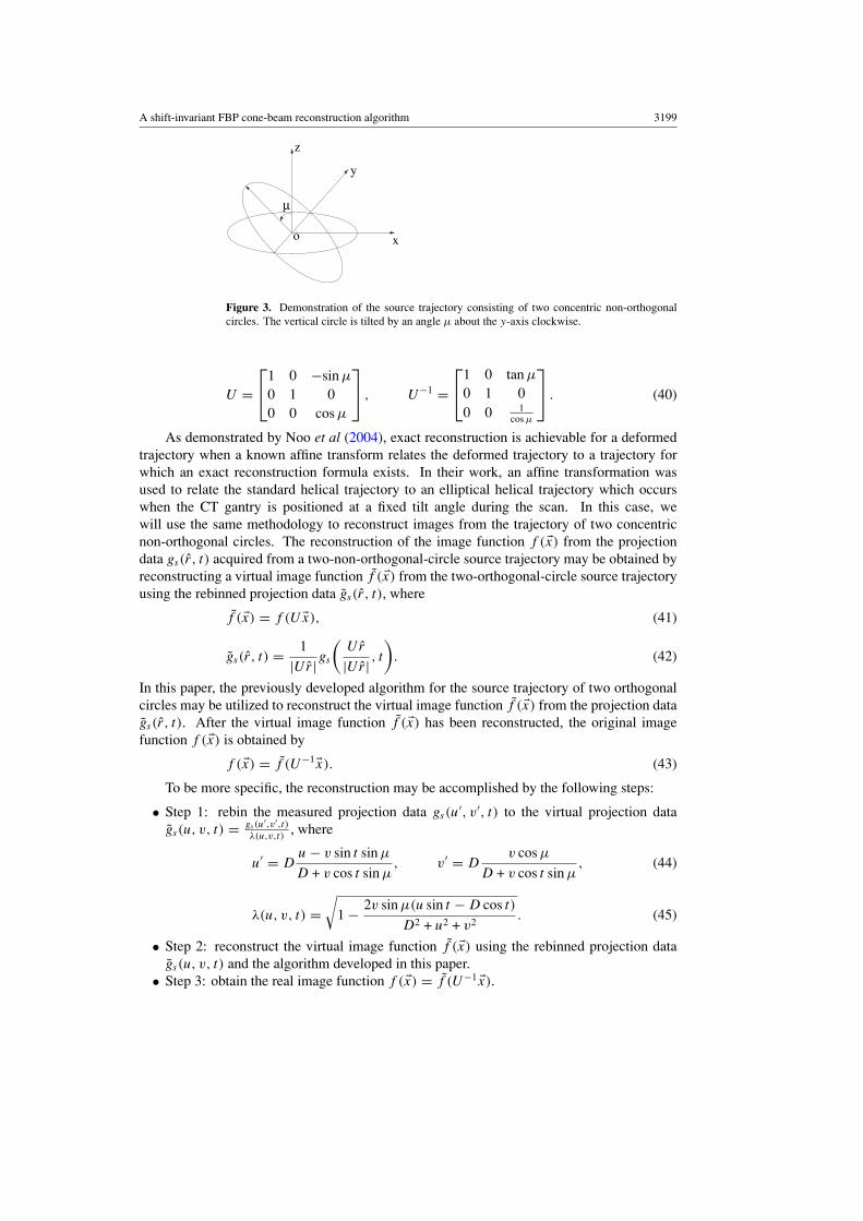
The second set of reconstruction results is presented to demonstrate the ability of thealgorithm to reconstruct a phantom which is theoretically challenging for a single circulartrajectory. A Defrise phantom has been reconstructed where several ellipsoids are stackedalong the z-axis (figures 5(a) and (b)). Density plots have also been provided in figures 5(c)and (d). As described above, the final reconstruction result is the sum of a contribution fromthe source trajectory in the x–y plane and in the y–z plane. These contributions are displayedseparately here so that one may assess the relative contribution from each of these two circlesto the final image. One may note that the reconstruction of the x–y plane contains nearly equalcontributions from each of the source trajectories. The more interesting case is that of thereconstruction of the x–z plane. The contribution from the horizontal circle displays artefactswhich are well known and encountered when reconstructing the Defrise phantom from asingle circular source trajectory. However, in this case the contribution from the verticalcircle actually compensates for these artefacts, as one may note by examining figures 5(b) and(d). Thus, in the portions of image space where the contribution from the horizontal circleoverestimates the true value of the phantom, the contribution from the vertical circle providesless positive values. This algorithm provides exact reconstruction from two orthogonal circleswhich satisfies the Tuy data sufficiency condition; thus, this type of compensation behaviouris anticipated so that the final combined image is an accurate reconstruction of the phantom.

A shift-invariant FBP cone-beam reconstruction algorithm 3201

Figure 4. The images provide a comparison between the theoretical phantom values (left column),the reconstructed values from noise-free projection data (centre column) and the reconstructedvalues using projection data with Poisson noise (right column). Images are displayed from thethree orthogonal planes defined in the text: the x–y plane (upper row), the y–z plane (centre row)and the x–z plane (lower row).

5.2. Reconstruction from non-orthogonal concentric circles

In order to validate the reconstruction algorithm presented here for the case of two concentricnon-orthogonal circles, further experimental simulations were performed. In this case, thetilt angle parameter was set as µ = 20◦. Sample projection data acquired using the Defrisephantom are given in figure 6. Note that the horizontal acquisition is unchanged and onlythe acquisition from the vertical circle has changed for this simulation of a non-orthogonalacquisition. The rebinned data are also demonstrated here and correspond to the projection of avirtual image object acquired from two concentric orthogonal circles. It is these rebinned datawhich are used to reconstruct, via the reconstruction formula for two concentric orthogonalcircles based on the procedure outlined above.

The third set of reconstruction results presented here corresponds directly to the first set,i.e. the positions of the reconstructed planes are identical. The difference between these twosets is that the first set was acquired from orthogonal concentric circles (µ = 0◦) and thesecond set was acquired from non-orthogonal concentric circles (µ = 20◦). These results areshown in figure 7 and are consistent with the claim that exact reconstruction is also achievedfor a non-orthogonal concentric circle acquisition. Additionally, the Defrise phantom wasreconstructed as shown in figure 8. The results are displayed in the same window and maybe compared with the final reconstruction results given in figure 5 for the case of orthogonalconcentric circles. Finally, density plots are provided for both the Shepp–Logan phantom andthe Defrise phantom (figures 9(a)–(e)) to demonstrate the quantitative reconstruction accuracyachieved with this exact algorithm.

3202 T Zhuang et al

(a)

(b)

50 100 150 200 250

0

0.2

0.4

0.6

0.8

1

Image Voxel Index

Rel

ativ

e D

ensi

ty

(c)

50 100 150 200 250−0.4

−0.2

0

0.2

0.4

0.6

0.8

1

1.2

Image Voxel Index

Rel

ativ

e D

ensi

ty

(d)

Figure 5. Reconstructed images from two orthogonal slices of the Defrise phantom aredemonstrated here. The x–y slice (z = 0.0039) is given in (a) with a display window [0, 1]and the x–z slice (y = 0.0039) is shown in (b) with a display window [−1, 1]. The contributionto the final reconstruction from the horizontal circular trajectory is given in the left-most images.The contribution to the final reconstruction from the vertical circular trajectory is given in thecentral images. The sum of these two contributions is the final reconstruction and is given in theright-most images. Density plots from vertical lines through the images in (a) and (b) are given in(c) and (d). The line plotted in (c) corresponds to (y = 0.0039, z = 0.0039) and the line plotted in(d) corresponds to (x = 0.0977, y = 0.0039). The theoretical expected result (blue dashed line),the horizontal contribution (black dash-dotted line), the vertical contribution (red dotted line) andthe final reconstructed result (green solid line) are plotted for comparison in each case.

A shift-invariant FBP cone-beam reconstruction algorithm 3203

Figure 6. Sample projection data of the Defrise phantom acquired for orthogonal and non-orthogonal concentric circles as well as the results of the rebinning operation. The acquired dataare shown where u is increasing from right to left and v is increasing from the bottom to the top.Likewise, in the rebinned data u′ is increasing from right to left and v′ is increasing from thebottom to the top. The two sample projections are taken from the view angles t = π/4 (in thehorizontal circle) and t = 9π/4 (in the vertical circle).

Figure 7. The images provide a comparison between the theoretical phantom values (left column),the reconstructed values from noise-free projection data (centre column) and the reconstructedvalues using projection data with Poisson noise (right column). Images are displayed from thethree orthogonal planes defined in the text: the x–y plane (upper row), the y–z plane (centre row)and the x–z plane (lower row).

3204 T Zhuang et al

(a) (b)

Figure 8. Reconstructed images from two orthogonal slices of the Defrise phantom are presentedhere. The x–y slice is given in (a) with a display window [0, 1] and the x–z slice is shown in(b) with a display window [−1, 1].

5.3. Numerical demonstration of the benefit of equal weighting

This algorithm was derived using an equal weighting scheme which is optimal with respectto the noise variance of the reconstruction algorithm and consequently optimal for doseminimization (Parker et al 1981). An overview of exact reconstruction formulae published inthe literature for circle-based trajectories will be given in the discussion section. In this section,we will compare the noise properties of this algorithm with one of the recently published shift-invariant FBP reconstruction formulae for the case of a circle–arc source trajectory (Katsevich2005). There are a couple of crucial differences between our algorithm and that given byKatsevich for the circle–arc source trajectory. The first difference is that in reconstructingany given image point the new algorithm presented here enables utilization of projectiondata collected from all view angles on the two concentric circles. In contrast, Katsevich’scircle–arc algorithm utilizes the geometric concept of generalized PI-lines (see the discussionsection for more details) and in reconstructing a given image point only uses data from a givenPI-segment of the source trajectory (referred to by Katsevich as the π -parametric interval ofthe image point) (Katsevich 2005). The second difference is that non-equal weighting of theredundantly measured projection data is used in the Katsevich algorithm, whereas redundantdata are given an equal weighting in this new algorithm. On the other hand, there areseveral similarities between these algorithms including shift-invariant filtering and a filteredbackprojection structure in which the data are first differentiated, Hilbert filtered along linesin the detector plane and then backprojected. Since identical implementation was used herefor the differentiation step and the filtering operation, an unbiased noise comparison may beconducted directly between this new algorithm and Katsevich’s circle–arc algorithm.

Numerical simulations using the Shepp–Logan phantom were performed in order toverify that this new algorithm will have improved noise characteristics. The same geometricparameters introduced above were utilized for this comparison. A volume of the Shepp–Logan phantom was reconstructed with both reconstruction algorithms with a total z extentof 0.5625 and the same image volume sampling given above. The noise response of thereconstruction algorithms has been assessed by subtracting the reconstruction results usingnoise-free projection data from the projection data with simulated Poisson noise. In thecase of the Katsevich algorithm for this geometry the total scan range in the x–y plane was11π

9 rad (this angular range fulfils the short scan condition) and the total scan range on thevertical circular trajectory was 8π

45 rad (this value is determined by the height of the volumeof interest). Thus, for this reconstruction the Katsevich algorithm only uses data from a total

A shift-invariant FBP cone-beam reconstruction algorithm 3205

50 100 150 200 2500.98

0.99

1

1.01

1.02

1.03

1.04

1.05

1.06

Image Voxel Index

Rel

ativ

e D

ensi

ty

50 100 150 200 2500.9

0.92

0.94

0.96

0.98

1

1.02

1.04

1.06

1.08

1.1

Image Voxel Index

Rel

ativ

e D

ensi

ty

50 100 150 200 2500.9

0.92

0.94

0.96

0.98

1

1.02

1.04

1.06

1.08

1.1

Image Voxel Index

Rel

ativ

e D

ensi

ty

50 100 150 200 250

0

0.2

0.4

0.6

0.8

1

Image Voxel Index

Rel

ativ

e D

ensi

ty

50 100 150 200 250

0

0.2

0.4

0.6

0.8

1

Image Voxel Index

Rel

ativ

e D

ensi

ty

(a) (b)

(c)

(e)

(d)

Figure 9. Density plots comparing the theoretical phantom values (solid line), the noiselessreconstruction results for two orthogonal circles (dotted line) and the noiseless reconstructionresults for two non-orthogonal circles (dashed line). The upper row of results corresponds to thelines shown in the central column of the images in figure 4: (a) density plot of a central horizontalline from the images in the upper row of figures 4 and 7 (x = 0.0039, z = 0.0039), (b) density plotof a vertical line from the images in the middle row (x = 0.0039, y = 0.0820), and (c) densityplot of a horizontal line from the images in the lower row (x = 0.0039, z = −0.2539). Thelower row of plots shown here correspond to the density plots from figures 5 and 8: (d) densityplot of a horizontal line from the x–y plane (y = 0.0039, z = 0.0039), and the line plotted in(e) corresponds to (x = 0.0977, y = 0.003 9).

3206 T Zhuang et al

(a) (b) (c)

(d) (e) (f)

Figure 10. Reconstructed images of the plane z = −0.246 are shown along with the purenoise images obtained after subtraction of the noiseless reconstruction to visually compare thenoise patterns of the reconstructed results: the results for the new algorithm (a), (d), the results forthe Katsevich algorithm with the total dose conserved (b), (e) and the Katsevich algorithm withthe dose per view angle conserved (c), (f).

angular range of 63π45 rad, whereas this new algorithm uses data from the complete 4π rad

of the two concentric circles. Due to this difference in data utilization of the algorithms,the comparison between this new algorithm and the Katsevich algorithm will be under twoseparate conditions. First, equal delivered dose from each view angle (N0 = 20 000 deliveredphotons per detector element) on the complete two-orthogonal-circle trajectory (i.e. 4π ).Second, equal delivered dose for the entire scan where the Katsevich algorithm has a reducedscan range. Therefore, in this comparison the effective dose per view angle will be increased(N0 = 57 143 delivered photons per detector element) for the Katsevich algorithm. Imagesfrom the reconstructed volumes are provided to compare the noise response of the algorithms(figure 10). In addition to the visual demonstration of the differences in noise response,quantitative comparisons have been made over the reconstructed volumes using the noisevariance as the statistic of interest. The noise variance was measured in the uniform backgroundportion of the Shepp–Logan phantom over the entire reconstructed volume and the resultsare summarized in table 1. These results demonstrate the dramatic dose penalty (factorof 4) which would occur if data were collected over two complete concentric circles andreconstructed using Katsevich’s circle–arc algorithm. This result is due primarily to thefact that many of the acquired view angles would not be utilized in Katsevich’s circle–arcalgorithm. The more interesting comparison is that of our new algorithm and Katsevich’scircle–arc algorithm under the condition of equivalent total dose. In that case, this new

A shift-invariant FBP cone-beam reconstruction algorithm 3207

Katsevich @ equivalent Katsevich @ equivalentThis algorithm total dose dose per view

σ 2 1.203 × 10−4 1.689 × 10−4 4.843 × 10−4

Effective dose savings – 1.40 4.03

algorithm achieves a dose advantage of 1.4 due solely to the utilization of the equal weightingscheme.

6. Discussion

Over the past decade, several cone-beam image reconstruction algorithms have been proposedfor circle-based source trajectories. Based upon Grangeat’s theory (Grangeat 1991), shift-variant filtered backprojection (FBP) algorithms were developed for source trajectoriesincluding circle plus arc (Wang and Ning 1999), circle plus two arcs (Tang and Ning 2001) andtwo orthogonal circles (Kudo and Saito 1994). Recently, a general shift-invariant FBP cone-beam reconstruction scheme has been discovered (Katsevich 2003, Chen 2003). Utilizingthis general framework, a flexible reconstruction algorithm was proposed by Katsevich forsource trajectories consisting of several circular segments (Katsevich 2005). For the samesource configurations, infinitely many other shift-invariant cone-beam image reconstructionalgorithms were also independently developed by utilizing a factorized weighting function(Chen et al 2005, Pack and Noo 2005). A different image reconstruction method viafiltering the backprojection image of differentiated projection data (FBPD) for a generalsource trajectory was discovered (Zou and Pan 2004a, 2004b, Zhuang et al 2004a, Pack etal 2005, Zhao et al 2005, Ye et al 2005). Several FBPD image reconstruction algorithmsfor the circle-based geometry have been obtained and implemented (Chen et al 2005,Zou et al 2005).

In order to place this new algorithm in the context of the existing analytic reconstructionalgorithms, we will highlight the differences between this algorithm and the existing algorithmsthat may take on a shift-invariant form. The source trajectory of two concentric circles hasthe geometric property of the existence of doubly measured (DM) lines (Chen et al 2005,Zou et al 2005, Pack et al 2005, Katsevich 2005); namely for a given image point withinthe reconstruction volume there will be at least one line which contains this point and alsoconnects two points on the source trajectory. These lines will be referred to as DM linesbut other investigators have also used the terms chords (Zou et al 2005), R-lines (redundantlymeasured) (Pack et al 2005) and PI-lines (Katsevich 2005). All of the published shift-invariantalgorithms for the circle-based trajectories to this point are based upon DM lines. One of thenovel contributions of this work is to provide a shift-invariant reconstruction formula for thetwo-concentric-circle trajectory which is not based on the properties of DM lines. Therefore,one difference between this algorithm and the algorithm obtained by Katsevich (2005) is thatthis algorithm enables the use of projection data from each view angle when reconstructingeach image point within the two concentric circles. Another feature of each of the publishedshift-invariant algorithms is that each of them involves negative weights when dealing withredundantly measured data. In this work, an equal weighting scheme is used to compensatefor the data redundancy; this weighting scheme does not introduce any negative weights. Theequal weighting scheme provides the optimal result from the standpoint of the noise in thereconstructed image (Parker et al 1981). Numerical simulations have been conducted andsupport our assertion that an equal weighting function should yield improved dose utilization.

3208 T Zhuang et al

7. Conclusions

A shift-invariant FBP algorithm for a source trajectory consisting of two concentric circleswhich may or may not be orthogonal has been presented. This algorithm utilizes an equalweighting scheme and was based on Katsevich’s general inversion scheme. The algorithm wasinitially derived for the case of two concentric orthogonal circles and generalized to the caseof two concentric non-orthogonal circles by applying an affine transformation. This trajectoryhas the desirable property that it will enable an exact reconstruction, as it satisfies Tuy’s datasufficiency condition. Key features of this algorithm include mathematical exactness, a shift-invariant filtered backprojection (FBP) structure, projection data from every source positionare utilized to reconstruct each image point and that an equal weighting scheme has beenutilized to efficiently account for redundantly measured data.

For the source trajectory of two concentric orthogonal circles, a symmetry property ofthis trajectory was utilized in order to simplify the calculation and implementation steps. Bydoing so, the identical steps used to compute the contribution to the reconstruction from thehorizontal circle were utilized for the vertical circle by simply permuting the coordinates ofthe image point used in the backprojection calculation. The reconstruction formula proceedsaccording to the following four steps. First, differentiate the cone-beam projection data withrespect to detector coordinates and source parameter. Second, pre-weight the differentiatedcone-beam data. Third, filter along three different orientations, determined by the structurefactor, using a 1D Hilbert kernel. These filtered data are linearly combined in order toobtain eight different filtration groups (four filtration groups in each circle). Each focal spoton the source trajectory is associated with a single filtration group. Finally, backprojectfrom each focal spot on the source trajectory using its associated filtration group, via avoxel-based three-dimensional backprojection operation from eight distinct backprojectionsets.

An affine transformation has been utilized to relate any source trajectory consisting oftwo concentric non-orthogonal circles to the source trajectory consisting of two concentricorthogonal circles. A general framework proposed by Noo et al (2004) was utilized to exactlyreconstruct image volumes from data acquired from non-orthogonal circles using the formuladeveloped for orthogonal circles. This algorithm proceeds according to the following steps.First, rebin the projection data so that they correspond to projections which would have beenacquired from a virtual image object via the two-orthogonal-circle source trajectory. Second,transform each reconstruction point to a virtual reconstruction point. Finally, perform the foursteps given above for the case of a two-orthogonal-circle trajectory.

In order to validate this algorithm, computer simulations have been performed usingthe standard low-contrast 3D Shepp–Logan phantom and the high-contrast Defrise phantom.Additionally, simulations including Poisson noise have been conducted and demonstrate thealgorithms improved dose utilization over previously published algorithms.

Acknowledgments

The work was partially supported by NIH grants 1R21 EB001683-01, 1R21 CA109992-01,5T32CA009206-24, a grant from University of Wisconsin-Madison and a grant from GEHealthcare Technologies. We acknowledge the use of open source code including AgnerFog’s random number generator and the Blitz++ templated array library. Thanks to OrhanUnal for his supervision of our computer network.

A shift-invariant FBP cone-beam reconstruction algorithm 3209

Appendix. The explicit expressions for sets T1( �x), T21( �x), T22( �x), T3( �x)

The sets are given by

T1( �x) ={(

π2 − θ1,

π2

) ∪ (3π2 , 3π

2 + θ2), x � 0,(

π2 , π

2 + θ1) ∪ (

3π2 − θ2,

3π2

), x � 0,

(A.1)

T21( �x) =

(3π2 + θ2,

3π2 + θ4

), x � 0, z � 0,(

π2 − θ3,

π2 − θ1

), x � 0, z � 0,(

π2 + θ1,

π2 + θ3

), x � 0, z � 0,(

3π2 − θ4,

3π2 − θ2

), x � 0, z � 0,

(A.2)

T22(x, y, z) = T21(x, y,−z), (A.3)

T3(�x) ={(

0, π2 − θ3

) ∪ (π2 , 3π

2

) ∪ (3π2 + θ4, 2π

), x � 0,(

0, π2

) ∪ (π2 + θ3,

3π2 − θ4

) ∪ (3π2 , 2π

), x � 0,

(A.4)

where

θ1(�x) = 2 sin−1

[ |x|√(r + y)2 + x2

],

θ2( �x) = 2 sin−1

[ |x|√(r − y)2 + x2

],

θ3(�x) = sin−1

[2|xr|√

(r2 + x2 − y2 − z2)2 + 4x2y2

]− sin−1

[2|x|y√

(r2 + x2 − y2 − z2)2 + 4x2y2

],

θ4( �x) = sin−1

[2|xr|√

(r2 + x2 − y2 − z2)2 + 4x2y2

]+ sin−1

[2|x|y√

(r2 + x2 − y2 − z2)2 + 4x2y2

].

(A.5)

References

Chen G H 2003 An alternative derivation of Katsevich’s cone-beam reconstruction formula Med. Phys. 30 3217–26Chen G H, Mistretta C A, Rowley H and Van Lysel M 2003 X-ray system for use in image guided procedures

US Patent Specification 0251010 (2005)Chen G H, Zhuang T, Leng S and Nett B E 2005 A showcase of exact cone-beam image reconstruction algorithms for

circle-based trajectories Proc. 8th Int. Meeting on Fully Three-Dimensional Image Reconstruction in Radiologyand Nuclear Medicine (Salt Lake City, UT) pp 295–9

Grangeat P 1991 Mathematical framework of cone beam 3D reconstruction via the first derivative of the Radontransform Mathematical Methods in Tomography (Lecture Notes in Mathematics vol 1497) ed G T Herman,A K Louis and F Natterer (New York: Springer) pp 66–97

Kak A C and Slaney M 1988 Principles of Computerized Tomographic Imaging (Bellingham, WA: IEEE)Katsevich A 2003 A general scheme for constructing inversion algorithms for cone-beam CT Int. J. Math. Sci.

21 1305–21Katsevich A 2005 Image reconstruction for the circle-and-arc trajectory Phys. Med. Biol. 50 2249–65Kudo H and Saito T 1994 Derivation and implementation of a cone-beam reconstruction algorithm for nonplanar

orbits IEEE Trans. Med. Imaging 13 196–211Noo F, Defrise M and Kudo H 2004 General reconstruction theory for multislice x-ray computed tomography with a

gantry tilt IEEE Trans. Med. Imaging 23 1109–16Noo F, Pack J and Heuscher D 2003 Exact helical reconstruction using native cone-beam geometries Phys. Med.

Biol. 48 3787–818Pack J D and Noo F 2005 Cone-beam reconstruction using 1D filtering along the projection of M-lines Inverse

Problems 21 1105–20

3210 T Zhuang et al

Pack J D, Noo F and Clackdoyle R 2005 Cone-beam reconstruction using backprojection of locally-filtered projectionsIEEE Trans. Med. Imaging 24 70–85

Pack J D, Noo F and Kudo H 2004 Investigation of saddle trajectories for cardiac CT imaging in cone-beam geometryPhys. Med. Biol. 49 2317–36

Parker D L, Smith V and Stanley J 1981 Dose minimization in computed tomography overscanning Med. Phys.8 706–11

Tang X and Ning R 2001 A cone-beam filtered backprojection (CB-FBP) reconstruction algorithm for a circle-plus-two-arc orbit Med. Phys. 28 1042–55

Tuy H K 1983 An inverse formula for cone-beam reconstruction SIAM J. Appl. Math. 43 546–52Wang X and Ning R 1999 A cone-beam reconstruction algorithm for circle-plus-arc data-acquisition geometry IEEE

Trans. Med. Imaging 18 815–24Ye Y, Zhao S, H. Yu and Wang G 2005 A general exact reconstruction for cone-beam CT via backprojection-filtration

IEEE Trans. Med. Imaging 4 1190–8Zhao S, Yu H and Wang G 2005 A unified framework for exact cone-beam reconstruction formulas Med. Phys.

32 1712–21Zhuang T, Leng S, Nett B E and Chen G H 2004a Fan-beam and cone-beam image reconstruction via filtering the

backprojection image of differentiated projection data Phys. Med. Biol. 49 5489–503Zhuang T, Nett B E, Tang X and Chen G H 2004b A cone-beam FBP reconstruction algorithm for short-scan and

super-short-scan source trajectories Proc. SPIE 5565 566–76Zou Y and Pan X 2004a Exact image reconstruction on PI-lines from minimum data in helical cone-beam CT Phys.

Med. Biol. 49 941–59Zou Y and Pan X 2004b An extended data function and its generalized backprojection for image reconstruction in

helical cone-beam CT Phys. Med. Biol. 49 N383–7Zou Y, Pan X and Sidky E 2005 Theory and algorithms for image reconstruction on chords and within regions of

interest J. Opt. Soc. Am. A 22 2372–84