A Sensor Fault Diagnosis Scheme for a DC/DC Converter

used in Hybrid Electric Vehicles

Hiba Al-SHEIKH

Ghaleb HOBLOS

Nazih MOUBAYED

2

Overview

Examined power converter system

Hardware prototype

Converter Modelling

Proposed residual-based fault diagnosis scheme

Bank of extended Kalman filters

Generalized likelihood ratio test

Tuning using receiver operating characteristic curve

Conclusion and future perspectives

3

Recent advances in power electronics encouraged the development of new initiatives for Hybrid Electric Vehicles (HEVs) with advanced multi-level power electronic systems.

Power converters are intensively used in HEVs• convert power at different levels• drive various load• electric drives

4

Intensive use of power converters in modern hybrid vehicles

Need for efficient methods of condition monitoring and fault diagnosis

Reliability of the automotive electrical power system

5

Controller

Power Converters

Sensors

Machine AC Side

Common Electrical Faults in Electric Drive Systems

Connectors/ DC Bus

Power Converters

• high power• relatively low voltage

high current

increase thermal and electric stresses on the converter components and

monitoring sensors

6

Controller

Power Converters

Sensors

Machine AC Side

Common Electrical Faults in Electric Drive Systems

Connectors/ DC Bus

• AC current sensor• DC bus voltage sensor

Power Converters

Sensors

Sensor faults in a DC/DC power converter system used in HEV

7

7

Observer-based

Fault diagnosis methods

Knowledge-based methods

Analytical model-based methods

Signal-based methods

Fault Diagnosis Techniques for Power Converters

Analytical model-based methods

For HEV applications where converters operate under variable load conditions, model-based diagnosis is of particular interest.

8

Examined Power Converter System

9

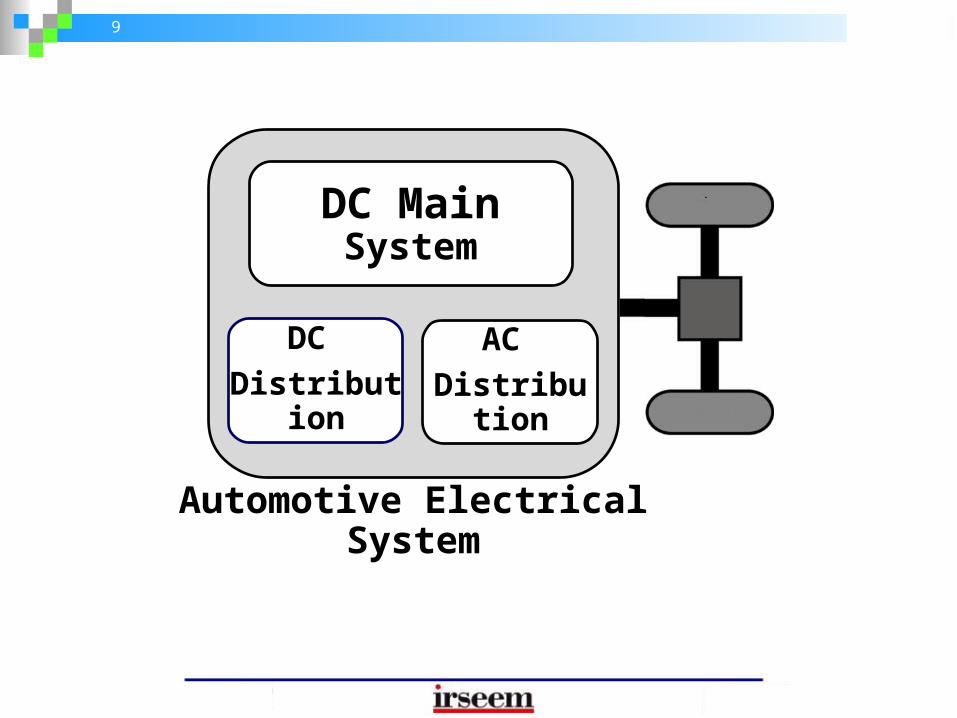
Automotive Electrical System

DC Main System

DC Distribution

AC Distribution

10

Power Converters DC/DC Choppers DC/AC Inverters AC/DC Rectifiers

Automotive Electrical System

11

12

13

Parallel DC-linked Multi-input DC/DC Converter consisting of two bidirectional half-bridge cells

DC bus

Energy Storage System AC Drive

BatteryPM

UC

Multi-port DC/DC

Converter

Inverter

Examined Power Converter System

14

Isolated topologies

boost-half bridge half-bridge full-bridge

Non-isolated topologies

SEPIC cuk buck-boost

Bidirectional DC/DC Converter Topologies

15

Source voltage 200VDC-link voltage 300V

Rated Power 30kWSwitching frequency 15kHzSource voltage ripple 2% p/pDC-link voltage ripple 4.5% p/p

Inductor current ripple ±10%

Design Requirements

Examined Power Converter System

Converter ParametersParameter Symbol Value

Input Capacitance Cin 80µFInput Capacitor ESR RCin 100mΩ

Inductance L 146µHInductor ESR RL 5mΩ

Output Capacitance Co 5mFOutput Capacitor ESR RCo 80mΩ

Transistor ON resistance RON 1mΩ

16

Examined Power Converter System

State variables

s

(duty cycle)

17

0 0.02 0.04 0.06 0.08 0.1194

196

198

200

x 1=v Cin

0 0.02 0.04 0.06 0.08 0.10

200

400

600

x 2=i L

0 0.02 0.04 0.06 0.08 0.1100

200

300

400

time (sec)

x 3=v Co

0 0.02 0.04 0.06 0.08 0.10

200

400

600

y 1=i in

0 0.02 0.04 0.06 0.08 0.1150

200

250

300

350

y 2=v o

time (sec)

State variables during healthy boost operation

Observed variables during healthy boost operation

18

Hardware Prototype of Converter System

19

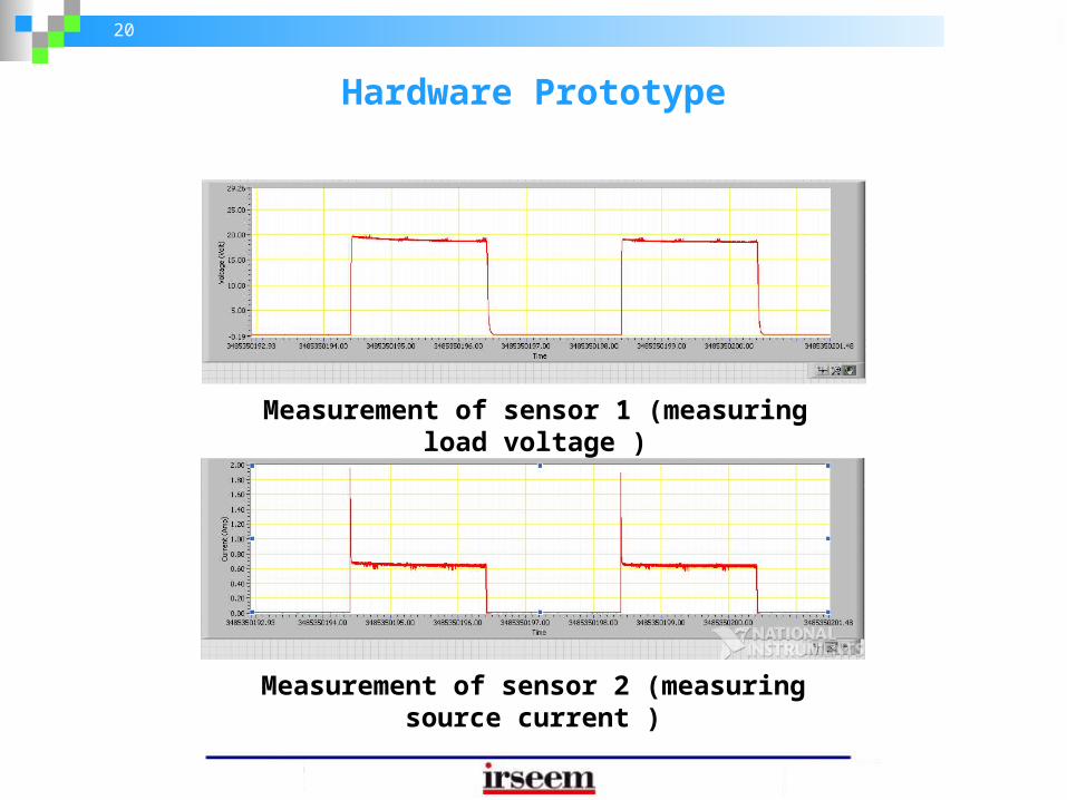
Hardware Prototype

Experimental test bench Hardware prototype of bidirectional DC/DC converter

20

Measurement of sensor 1 (measuring load voltage )

Measurement of sensor 2 (measuring source current )

Hardware Prototype

21

Sensor 2 Sensor 1

Hardware Prototype

22

Modelling of Power Converter

23

Converter State-Space Model

The examined converter is a nonlinear and time-varying system

DC busBatteryPM

UC

Multi-input DC/DC

Converter

Inverter

Boost operation

24

Converter State-Space Model

The examined converter is a nonlinear and time-varying system

DC busBatteryPM

UC

Multi-input DC/DC

Converter

Inverter

Buck operation

25

Converter State-Space Model

The examined converter is a nonlinear and time-varying system

The converter state-space model is obtained in three steps:

1. Piece-wise linear state-space model2. Continuous-time nonlinear state-space model3. Discrete-time nonlinear state-space model

26

Switching configuration 2 (T1 OFF; D2 ON) Switching configuration 2 (T2 OFF; D1 ON)

Switching configuration 1 (T1 ON; D2 OFF) Switching configuration 1 (T2 ON; D1 OFF)

Converter State-Space Model

Boost mode Buck mode

1. During each switching configuration, the converter is linear and possesses a piece-wise switched linear state-space model

27

Converter State-Space Model

1. During each switching configuration, the converter is linear and possesses a piece-wise switched linear state-space model

Operation Mode

Switching State

T1 D1 T2 D2

j = 1 (Boost)

i = 1 ON OFF OFF OFF

i = 2 OFF OFF OFF ON

j = 2 (Buck)

i = 1 OFF OFF ON OFFi = 2 OFF ON OFF OFF

28

Converter State-Space Model

Operation Mode

Switching State

T1 D1 T2 D2

j = 1 (Boost)

i = 1 ON OFF OFF OFF

i = 2 OFF OFF OFF ON

j = 2 (Buck)

i = 1 OFF OFF ON OFFi = 2 OFF ON OFF OFF

where

averaged using as control variable

2. Averaged continuous-time model

29

Converter State-Space Model

2. Averaged continuous-time model

The continuous-time model is nonlinear The duty cycle is a function of the state variables, is obtained from the converter dynamics during steady state

where

30

01

0

11

01

o

iCin

iCinCoiCinONiCinLCinin

iCin

in

iCinin

in

iCinin

C

fL

f

LR

RRfRRfRRRR

LR

RRC

R

RC

x

xxxxAav

o

Co

iCin

Cin

iCinin

C

L

Rf

LR

RRC

10

1

01

xxB av

110

01

Co

iCin

Cin

iCin

RfR

R

Rx

xCav

Co

iCin

RR0

01

avD

.

Converter State-Space Model

31

Converter State-Space Model

3. The continuous-time model is discretized using first order hold with sampling period seconds.

Including process noise and measurement noise, the discrete-time state-space model becomes

and are white Gaussian, zero-mean, independent random processes with constant auto-covariance matrices Q and R.

32

Proposed Fault Diagnosis Algorithm

33

Fault Diagnosis of Converter Sensor Faults

Sensor 2

Sensor 1

Model-Based Residual Approach

34

Output variables

Input variables

Power Converter System

Residual Generation

Fault/No fault

Residual Evaluation

Residuals

Fault Diagnosis of Converter Sensor Faults

35

Residual Generation using Bank of Extended Kalman Filters

36

Converter state-space model

+ +

Converter input signals

Sensor measured signals

The Extended Kalman Filter (EKF)

Estimates of the measured signals ∑

+

- Residual signals“Innovations”

37

The Extended Kalman Filter (EKF)

Recursive application of prediction and correction cycles

At the end of sampling period, the nonlinearity of the converter system is approximated by a linear model around the last predicted and corrected estimate

38

The EKF Algorithm

Initialization and

Prediction Cycle

where is the jacobian matrix of

Correction CycleA new measurement is obtained

where is the jacobian matrix of

incrementsPrediction and correction repeat with corrected estimates used to predict new estimates

39

0 0.01 0.02 0.03 0.04 0.05

0

100

200

300

400Observer 1

time (s)

Resid

ual r

1 ey1

0 0.01 0.02 0.03 0.04 0.05

-50

0

50

100

150

time (s)

Resid

ual r

1 ey2

0 0.01 0.02 0.03 0.04 0.05-100

0

100

200

300Observer 2

time (s)

Resid

ual r

2 ey1

0 0.01 0.02 0.03 0.04 0.05-4

-2

0

2

4

time (s)

Resid

ual r

2 ey2

Residuals Generated by the Bank of EKF

Instant of fault

Standardized residuals with fault on sensor 1 occurring at 0.03s

40

0 0.01 0.02 0.03 0.04 0.05-4

-2

0

2

4Observer 1

time (s)

Resid

ual r 1 e

y1

0 0.01 0.02 0.03 0.04 0.05

0

500

1000

1500

2000

2500

time (s)

Resid

ual r 1 e

y2

0 0.01 0.02 0.03 0.04 0.05

0

500

1000

1500

2000

2500Observer 2

time (s)

Resid

ual r 2 e

y1

0 0.01 0.02 0.03 0.04 0.05

0

500

1000

1500

2000

2500

time (s)

Resid

ual r 2 e

y2

Standardized residuals with fault on sensor 2 occurring at 0.03s

Instant of fault

Residuals Generated by the Bank of EKF

41

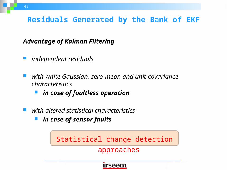
Residuals Generated by the Bank of EKF

Advantage of Kalman Filtering

independent residuals

with white Gaussian, zero-mean and unit-covariance characteristics in case of faultless operation

with altered statistical characteristics in case of sensor faults

Statistical change detection approaches

42

Residual Evaluation using Generalized Likelihood Ratio Test

43

Residuals Evaluation Approaches

Statistical data processing

Correlation

Pattern recognition

Fuzzy logic

Fixed threshold

Adaptive threshold Stochastic envirmonent

Likelihood ratio tests

Generalized Likelihood Ratio (GLR) Test

44

Residuals Evaluation using GLR Test

sensor is faultless residuals are Gaussain

with and

sensor is faulty is altered into and

into

Statistical Hypothesis Testing ProblemHo and H1

45

Statistical Hypothesis Testing ProblemHo and H1

Residuals Evaluation using GLR Test

Maximizing the likelihhod ratio

is the Maximum Likelihood Estimate (MLE) of is the MLE of

ooy

y

y Hep

HepeL

i

i

i ,ˆ;

,ˆ;ln

11

46

At every time step t

Apply the GLR statistic on the recent W residual values

Generate a detection function for each residual

Is residual variance known?

Evaluate for all using

2

)(

2

kxk

kGLR tt

Evaluate for all using

2

)(

)(1ln

2 k

kxkkGLR

t

tt

Is ?Decide H1

(fault)Decide H0

(No fault)

Yes No

Yes No

GLR Algorithm

47

Detection Function Generated by GLR Test

Detection function with fault on sensor 1

0 0.01 0.02 0.03 0.04 0.05

0

100

200

300

Residual r1 e

y1

0 0.01 0.02 0.03 0.04 0.05-5

0

5

Residual r2 e

y2

0 0.01 0.02 0.03 0.04 0.050

10

20

30

GLRt for r

1 e

y1

0 0.01 0.02 0.03 0.04 0.050

10

20

GLRt for r

2 e

y2

0 0.01 0.02 0.03 0.04 0.050

10

20

30

time (s)

GLRt for r

1 e

y1

0 0.01 0.02 0.03 0.04 0.050

10

20

time (s)

GLRt for r

2 e

y2

instant of fault

unknown

known known

unknown

48

Detection Function Generated by GLR Test

Detection function with fault on sensor 2

0 0.01 0.02 0.03 0.04 0.05-5

0

5

Residual r1 e

y1

0 0.01 0.02 0.03 0.04 0.050

2

4

GLRt for r

1 e

y1

0 0.01 0.02 0.03 0.04 0.050

20

40

GLRt for r

2 e

y2

0 0.01 0.02 0.03 0.04 0.050

1

2

3

time (s)

GLRt for r

1 e

y1

0 0.01 0.02 0.03 0.04 0.050

20

40

time (s)

GLRt for r

2 e

y2

0 0.01 0.02 0.03 0.04 0.05

0

1000

2000

Residual r2 e

y2

instant of fault

unknown

known

unknown

known

49

Tuning using Receiver Operating Characteristic Curve

50

false positives rate (tpr)

true

pos

itive

s ra

te (f

pr)

(0, 0)

(1, 1)

as increase

0 1

1

+ optimal

ROC Analysis

An evaluation tool to measure the performance of the residual-based GLR test.

51

Three ROC Plots: W = 30

For each W, is varied from 0 to

For each , a test set of 1000 simulations is used

Healthy and faulty trials

During faulty trials, different fault amplitudes were injected

At the end of every trial, the detection function is generated using and compared the corresponding

At the end of the 1000 trials, the tpr and fpr are calculated and the corresponding point is located on the ROC curve.

ROC Analysis

W = 50 W = 70

52

-1 0 1 2 3 4 5 6 7

x 10-3

0.97

0.98

0.99

1

28.62

28.57

28.5628.55

28.5428.53

28.5228.51

28.5

28.49

28.48

28.47

28.46

28.45

28.44

28.43

28.42

28.41

28.4

28.39

28.38

28.37

28.36

28.35

28.34

28.33

28.32

28.31

28.3

28.29

28.28

28.27

28.26

28.25

28.24

28.23

28.22

28.21

28.2

28.19

28.18

28.17

28.16

28.14

28.13

28.11

28.1

28.0828.05 21.56 21.24 20.31 19.8 17.88 17.63 17.39 16.35 14.9 14.8 14.49 14.48 14.42 14.41 14.22 14.19 14 13.89 13.81 13.48 13.43 13.41 13.09 13.05 13.01 12.95 12.71 12.06 12.01 11.97 11.96 11.91 11.75 11.73 11.65 11.56 11.51 11.46 11.45 11.44 11.34 11.29 11.24 11.2 11.18 11.17 11.01 10.98 10.96 10.89 10.87 10.75 10.72 10.61 10.57 10.54 10.49 10.34 10.31 10.28 10.13 10.05 10 9.93 9.91 9.86 9.85 9.84 9.8 9.6 9.58 9.56 9.55 9.3 9.22 9.2 9.14 9.04 9.03 9.01 8.99 8.98 8.97 8.94 8.89 8.88 8.79 8.78 8.73 8.71 8.63 8.57 8.55 8.54 8.52 8.51 8.48 8.46 8.44 8.38 8.35 8.34 8.33 8.31 8.29 8.22 8.2 8.16 8.15 8.13 8.12 8.02 8.01 8 7.95 7.91 7.85 7.82 7.78 7.76 7.73 7.71 7.7 7.69 7.68 7.63 7.61 7.6 7.56 7.53 7.48 7.47 7.37 7.32 7.27 7.21 7.19 7.16 7.14 7.06 7.05 7.04 7.03 7 6.99 6.97 6.95 6.93 6.91 6.9 6.88 6.86 6.84 6.83 6.81 6.79 6.78 6.76 6.74 6.72 6.71 6.7 6.69 6.68 6.66 6.64 6.62 6.61 6.59 6.58 6.57 6.56 6.55 6.54 6.52 6.51 6.49 6.47 6.46 6.43 6.38 6.36 6.35 6.33 6.31 6.3 6.28 6.27 6.25 6.23 6.21 6.2 6.19 6.18 6.17 6.16 6.15 6.14 6.13 6.09 6.07 6.05 6.04 6.01 5.99 5.98 5.97 5.96 5.95 5.94 5.93 5.92 5.9 5.89 5.87 5.84 5.8 5.77 5.75 5.73 5.71 5.7 5.69 5.68 5.66 5.65 5.64 5.61 5.6 5.59 5.58 5.57 5.56 5.55 5.54 5.52 5.5 5.49 5.47 5.46 5.45 5.44 5.43 5.42 5.41 5.36 5.35 5.34 5.32 5.31 5.3 5.29 5.28 5.27 5.25 5.24 5.21 5.18 5.17 5.14 5.12 5.11 5.1 5.08 5.06 5.05 5.03 5.02 5.01 5 4.96 4.95 4.92 4.87 4.86 4.854.84 4.83 4.82 4.78 4.76 4.75 4.74 4.73 4.71 4.7 4.68 4.63 4.61 4.59 4.56 4.55 4.54 4.53 4.52 4.51 4.5 4.48 4.46 4.43 4.42 4.41 4.4 4.37 4.35 4.31 4.29 4.28 4.26 4.25 4.24 4.21 4.19 4.18 4.16 4.15 4.14 4.13 4.12 4.1 4.09 4.08 4.07 4.06 4.05 4.04 4.03 4.02 4 3.98 3.97 3.96 3.95 3.94 3.93 3.92 3.91 3.9 3.88 3.86 3.83 3.82 3.81 3.8 3.78 3.77 3.76 3.72 3.71 3.7 3.69 3.65 3.64 3.63 3.62 3.61 3.6 3.56 3.55 3.54 3.53 3.51 3.5 3.49 3.47 3.46 3.43 3.4 3.38 3.36 3.35 3.31 3.3 3.27 3.25 3.23 3.22 3.16 3.12 3.11 3.1 3.09 3.08 3.07 3.06 3.05 3.04 3.03 3.02 3.01 3 2.99 2.97 2.96 2.95 2.94 2.93 2.92 2.91 2.9 2.89 2.88 2.87 2.86 2.85 2.84 2.82 2.81 2.79 2.78 2.73 2.72 2.68 2.65 2.63 2.62 2.6 2.59 2.58 2.57 2.54 2.53 2.51 2.5 2.48 2.46 2.45 2.44 2.43 2.41 2.4 2.39 2.37 2.34 2.32 2.29 2.26 2.24 2.23 2.21 2.2 2.19 2.18 2.17 2.16 2.14 2.13 2.11 2.09 2.08 2.05 2 1.99 1.97 1.96 1.94 1.93 1.92 1.9 1.89 1.88 1.84 1.79 1.77 1.76 1.65 1.64 1.62 1.61 1.55 1.54 1.53 1.52 1.51 1.4 1.39 1.38 1.37 1.3 1.27 1.25 1.22 1.2 1.16 1.12 1

0 5 10 15 20

x 10-3

0.94

0.96

0.98

1

X: 0Y: 1

ROC curve (Observer 1/ Residual 1) r1e

y1

false positive rate

true

posit

ive ra

te

X: 0.002894Y: 1 X: 0.0152

Y: 0.9942

W=30

W=50

W=70

optimal point (0,1)

-1 0 1 2 3 4 5 6 7

x 10-3

0

0.2

0.4

0.6

0.8

1

35.3535.34

35.33

35.3235.31 34.83 31.43 30.66 29.71

28.99 28.97 28.39 28.35 27.96 27.95 27.71 27.14 26.71 26.68 26.66 26.3 25.62 25.53 25.17 24.69 24.66 24.42 24.2 24.01 24 23.58 23.34 23.23 23.18 22.73 22.69 22.59 22.49 22.38 22.36 22.28 21.87 21.75 21.72 21.59 21.4 21.2 20.87 20.59 20.49 20.28 20.01 19.8 19.78 19.66 19.65 19.61 19.52 19.48 19.47 19.24 19.01 19 18.92 18.91 18.69 18.66 18.48 18.33 18.27 18.13 18.06 18.01 18 17.98 17.92 17.75 17.63 17.49 17.45 17.38 17.33 17.28 17.25 17.24 17.21 17.16 17.12 17.08 16.75 16.69 16.68 16.61 16.55 16.42 16.39 16.29 16.22 16.15 16.13 16.12 16.01 15.9 15.85 15.83 15.82 15.8 15.72 15.69 15.59 15.58 15.57 15.48 15.39 15.38 15.27 15.24 15.2 15.13 15.09 15.05 15.01 14.93 14.89 14.85 14.78 14.76 14.64 14.63 14.48 14.41 14.4 14.36 14.34 14.31 14.29 14.15 14.13 14.03 14.02 14.01 13.98 13.9 13.82 13.81 13.78 13.77 13.74 13.64 13.59 13.55 13.54 13.52 13.39 13.36 13.31 13.3 13.27 13.23 13.21 13.03 13.02 12.98 12.97 12.96 12.93 12.91 12.88 12.83 12.77 12.65 12.64 12.61 12.59 12.58 12.42 12.4 12.32 12.29 12.28 12.24 12.22 12.17 12.08 12.05 12.01 11.97 11.93 11.92 11.89 11.88 11.85 11.83 11.82 11.79 11.75 11.74 11.65 11.61 11.55 11.47 11.42 11.41 11.38 11.35 11.33 11.31 11.3 11.21 11.2 11.17 11.16 11.14 11.13 11.1 11.08 11.07 11.04 11.03 11 10.98 10.96 10.93 10.92 10.91 10.88 10.85 10.84 10.82 10.81 10.73 10.7 10.64 10.63 10.62 10.59 10.56 10.54 10.51 10.49 10.46 10.42 10.4 10.37 10.36 10.35 10.32 10.3 10.23 10.19 10.18 10.17 10.11 10.1 10.08 10.05 10.04 10.03 10.02 10 9.99 9.97 9.96 9.93 9.82 9.75 9.74 9.7 9.68 9.62 9.58 9.56 9.55 9.5 9.49 9.46 9.41 9.4 9.31 9.29 9.28 9.27 9.25 9.24 9.22 9.2 9.19 9.16 9.15 9.12 9.11 9.05 9.01 8.97 8.94 8.92 8.91 8.85 8.84 8.8 8.79 8.78 8.73 8.72 8.68 8.67 8.63 8.62 8.6 8.59 8.58 8.56 8.55 8.52 8.5 8.48

-0.005 0 0.005 0.01 0.015 0.02 0.025 0.03 0.035 0.040.6

0.7

0.8

0.9

1

X: 0Y: 1

ROC curve (Observer 2/ Residual 2) r2e

y2

false positive rate

true

posit

ive ra

te

X: 0.01333Y: 1

X: 0.0304Y: 1

W=30

W=50

W=70

optimal point (0,1)

ROC Curve for Residual r1ey1 ROC Curve for Residual r2ey2

false positive rate false positive rate

true

pos

itive

rate

true

pos

itive

rate

optimal point for =28.05 and =70 optimal point for =35.31 and =70

53

Conclusion and Future Perspectives

54

Proposed Fault Diagnosis Algorithm

Output variables

Input variables

Power Converter System

Bank of Kalman Filters

GLR Test

Residuals

Decision

Fault/No fault

Tuning of W

Tuning of

ROC curve Detection function

Residual Generation

Residual Evaluation

55

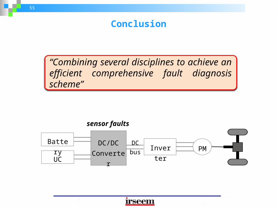
Conclusion

“Combining several disciplines to achieve an efficient comprehensive fault diagnosis scheme”

BatteryPM

UC

DC/DC Converter

InverterDC bus

sensor faults

56

Conclusion

GLR Test

+ +

Model-based Residual

generation

Power Converter Process

ROC Curves

57

« Power electronics interface configurations for hybrid energy storage in hybrid electric vehicles »

17th IEEE MELECON’14 Mediterranean Electrotechnical Conference

« Modeling, design and fault analysis of bidirectional DC-DC converter for hybrid electric vehicles »

23rd IEEE ISIE’14 International Symposium on Industrial Electronics

« Study on power converters used in hybrid vehicles with monitoring and diagnostics techniques »

17th IEEE MELECON’14 Mediterranean Electrotechnical Conference

« Condition Monitoring of Bidirectional DC-DC Converter for Hybrid Electric Vehicles »

22nd MED’14 Mediterranean Conference on Control & Automation

58

« A Sensor fault diagnosis scheme for a DC/DC converterused in hybrid electric vehicles »

9th IFAC Symposium on Fault Detection, Supervision and Safety for Technical Processes SAFEPROCESS'15

59

Future Perspectives

Future work will utilize the proposed model-based approach to detect/diagnose component faults in the converter such as

open-circuited transistor short-circuited diode degraded capacitor

60

Thank you