A Semi-Automated Decision Support Tool for Requirements Trade-off Analysis

Golnaz ElahiDepartment of Computer Science, University of Toronto

gelahi@cs.toronto.edu

Eric YuFaculty of Information, University of Toronto,

yu@ischool.utoronto.ca

Abstract—System designers and requirements analysts facemany competing requirements, such as performance, usabil-ity, security, cost, and so forth. To make trade-offs amongrequirements, ideally analysts would like to quantitativelymeasure consequences of alternative solutions on requirements.However, during the early stages of requirements and systemdesign, it is hard to quantitatively measure all factors andquantify stakeholders’ preferences. The Even Swaps method isa technique developed in management science to assist in multi-criteria decision making which allows the use of available butpotentially incomplete quantitative and qualitative measures. Itteases out the need to elicit importance weights of requirements.Instead, stakeholders are asked how much they would relax oneobjective to better achieve another. We apply the Even Swapstechnique to requirements trade-offs, and supplement it withan algorithm that automates the decision analysis process. Thealgorithm ns the most distinguishable pair of alternatives andsuggests the next requirements to be swapped to stakeholders.

Keywords-Requirement Trade-offs, Decision Analysis, Alter-native Design Solution, Even Swaps.

I. INTRODUCTION

Requirements analysts need to make key decisions earlyin the project, such as which architectural or design solutionto employ [1]. Each alternative solution satis es differ-ent functional and non-functional requirements to varyingextents. For example, if between two alternatives, one isexpensive with a high quality, and the other one has a betterprice with a low quality, which solution should be picked?Deciding on a solution requires making trade-offs amongrequirements with respect to consequences of alternativeson the requirements and preferences of stakeholders.

Ideally, analysts would like to quantitatively measure(estimate) consequences of alternative solutions on variousrequirements. However, while some requirements can bere ned into measurable variables, many non-functional re-quirements have a soft nature, which makes them hard, if notimpossible, to measure. Such requirements are treated as softgoals in some Requirements Engineering (RE) techniques,e.g., i* [2] and Tropos [3]. Goal model evaluation techniquessuch as [4], [5], [6], enable reasoning about the partialsatisfaction of soft goals by propagating qualitative labelssuch as partially satis ed ( ), suf ciently satis ed ( ),partially denied ( ), and fully denied ( ). In some other REapproaches, requirements and alternatives are quanti ed byusing ordinal measures or a probabilistic layer for reasoningabout partial goal satisfaction [7], [8], [9], [10].

Stakeholders may choose to evaluate some requirementsnumerically, and some requirements qualitatively, on dif-ferent scales, e.g., absolute values, percentages, ordinalnumbers, or qualitative labels. When different requirementsare measured (or estimated) on different scales, normalizinginconsistent types of measures into a single scale is trou-blesome and may not result in a meaningful utility value.Besides, extracting correct numerical importance weightscan be time-consuming and labor-intensive, specially whenthe number of criteria grows.

In summary, the main problems when making trade-offsamong requirements and deciding over alternative designsolutions are:

1) Extensive Data Collection: eliciting required informa-tion to make an objective decision usually involves anextensive data collection from stakeholders.

2) Manual Prioritization: extracting stakeholders’ pref-erences over multiple criteria in terms of numericalimportance weights is error-prone and labor-intensive.

3) Incomparable Scales: aggregating requirements mea-sures in different scales is usually error-prone or notpossible.

4) Scalability: the decision problem may become com-plicated and impossible to be analyzed manually dueto numerous requirements and/or alternatives.

Some decision analysis methods evaluate consequencesof alternative solutions in terms of precise and meaningfulquantitative measures [1], [7], [11]. Some decision analysisapproaches such as Analytical Hierarchy Process (AHP)[12] and Even Swaps [13] circumvent the need to measurerequirements and consequences of solutions. AHP worksbased on pairwise comparisons of all decision elements.Even Swaps is a recently introduced decision analysismethod in management science that consists of a chain oftrading one decision criterion for another. These trades arecalled swapping. Swaps are even, which means stakeholdersare asked to hypothetically improve one criterion, and inreturn, reduce another one proportionally (evenly).

We adopt the Even Swaps multi-criteria decision analysisapproach [13] to make trade-offs among requirements. Sincethe Even Swaps method works by trading-off one require-ment for another, importance weights of requirements are notneeded for determining the best solution. Requirements canbe evaluated in a mixture of scales and by different measure-

ment methods. Extensive data collection from stakeholders,as AHP works, are avoided.

This paper introduces a set of guidelines and a toolfor tailoring and enhancing the Even Swaps process forrequirements trade-off analysis. Although the Even Swapsmethod solves the problem 1, 2, and 3 (mentioned above),it may fail in practice due to scalability issues: when severalsoftware requirements and alternative solutions need to beconsidered, decision stakeholders can become overwhelmedor confused in making the best swap among numerouspossibilities [14]. Selecting two alternatives among manyoptions for the swapping process is also challenging. Themain contribution of this paper is introducing an algorithmand tool that:

• Semi-automates the Even Swaps process, in the sensethat the process is still interactive with stakeholderswhile being performed and controlled by an automatedalgorithm.

• Decides which pair of alternatives to compare in eachstep.

• Suggests the requirements to swap for analyzing eachpair of alternatives.

This paper is organized as follows. In Section II, weintroduce an example scenario to illustrate and motivate theproblems. Section III introduces basics of the Even Swapsmethod. Section IV presents details and the algorithm. Sec-tion V presents the results of some case studies of applyingthe proposed algorithm. In Section VI, some assumptionsmade in the algorithm are explained and feasibility of themethod is discussed. Section VII overviews the relatedwork, and nally Section VIII draws some conclusions anddiscusses the limitation of the method.

II. MOTIVATING EXAMPLE

The Example Scenario. We motivate our work with ascenario at the Ministry of Transportation, Ontario (MTO),Canada. Traf c Monitoring Centres (TOC) of MTO re-ceive traf c video feeds from cameras installed in Ontariohighways. TOC operators control and manage traf c byconstantly monitoring the ow of the traf c. Consider threehypothetical alternative Intelligent Transportation Systems(ITS): A1, A2, and A3.

Decision Criteria. To select a solution among alternativeITSs, decision stakeholders need to consider 9 main criteria,indicating costs, security level, usability, and performance ofeach proposal:

• T1: Time between a change in the trafficand notifying the operator

• T2: Time between requesting a feedand showing the video on the monitor

• S1: Authorized control of cameras• P1: Percentage of the time cameras areconnected

• G1: Easy to view the video feeds

Table ITHE CONSEQUENCE TABLE OF ALTERNATIVE ITS FOR THE MTO

SCENARIO

• G2: Easy to locate the cameras on theroad

• G3: Easy to change the cameras settings• C1: Cost of implementation• C2: Maintenance costs

Some of these factors are measurable; for example, theimplementation cost of solutions is known and performancecan be accurately estimated. On the other hand, the securitylevel and usability of these design solutions are not nu-merically measurable until the system is actually deployed.T1 and T2 are measurable performance variables; S1 is asecurity goal that is not directly measurable; P1 is securityvariable; G1, G2, and G3 are usability goals; and C1 andC2 are cost factors.

Consequence Table. We aggregate consequences of alter-natives on decision criteria in a table, which we refer to asthe consequence table. Table I shows the consequence tablefor A1, A2, and A3, and the impacts of these alternativeson the decision criteria. Table I also speci es which criterianeed to be minimized or maximized.

Consequence tables may contain heterogeneous data, i.e.,different goals can be evaluated on different scales and bydifferent techniques. Some of the criteria can be measur-able variables that need to be minimized or maximized.For example, in the case study scenario, stakeholders areable to estimate the Time between a change in thetraffic and notifying the operator (T1) in mil-liseconds based on the properties and speci cation of A1,A2, and A3. On the other hand, enough information is notavailable to quantitatively measure the Ease of changingcameras settings (G3), so they evaluate consequences ofA1, A2, and A3 on G3 by using qualitative labels of partiallysatis ed ( ), suf ciently satis ed ( ), partially denied ( ),and fully denied ( ). Some requirements are evaluated inthe ordinal scale of Low, Medium Low, Medium, MediumHigh, and High (which are abbreviated as L, ML, M, MH,and H respectively). We illustrate our method by analyzingtrade-offs among ITS requirements and selecting a solutionamong A1, A2, and A3.

III. BASICS OF THE EVEN SWAPS METHOD

The Even Swaps decision analysis method extracts stake-holders’ value trade-offs, i.e., how much stakeholders wouldgive up on one requirement for better satisfaction of another.For example, suppose two alternative solutions, A1 and A2

are compared based on their quality and price. The quality

of A1 is High, but it is an expensive solution, costing $20K.A2 costs $15K, but the quality of A2 is Medium:

Quality PriceA1 High $20KA2 Medium $15K

To select between A1 and A2, the analyst needs to makea trade-off between quality and price. Making this trade-off depends on stakeholders’ preferences. In this example,analysts need to understand how much stakeholders arewilling to pay for a High quality solution. In an even swap,analysts ask stakeholders a hypothetical question: If we couldimprove the quality of A2 from Medium to High, how muchyou would be willing pay for A2?

Let us assume stakeholders declare that they would bewilling to pay an extra $3K (in total $18K) for A2, if thequality of A2 is increased from Medium to High. A solutionwith High quality and price of $18K is not available. This isa virtual, hypothetical alternative which we call A′

2, and itis as preferred as A2, and can be used as its substitute. Nowdeciding between A1 and A′

2 is easier, because they bothhave a High quality, so the alternatives can be comparedwith respect to price only. Obviously, A′

2 is a better choice,and since A2 is as preferred as A′

2, we can conclude thatA2 should be preferred to A1.

Quality PriceA1 High $20K

A′2 = A2 High $18K

In an even swap, the decision analyst, collaborating withstakeholders, changes the consequence of an alternative onone requirement, and compensates this change with a pref-erentially equal change in the satisfaction level of anotherrequirement. Swaps aim to either make criteria irrelevant, inthe sense that both alternatives have equal consequences onthe criteria, or create a dominant alternative. Alternative A

dominates alternative B, if A is better than (or equal to) B

on every criteria [14]. Irrelevant attributes and dominated al-ternatives can both be eliminated, and the process continuesuntil only the most preferred alternative remains [14].

Remark In the rest of this paper, when a new conceptis de ned or general discussions are given, alternatives arenamed as A and B. The values of ax and bx denote thesatisfaction level of the requirements, gx, by alternatives A

and B.De nition 1. Consider alternative A and two require-

ments, gx and gy , where A satis es gx and gy at the levelof ax and ay. Swapping two requirements like gx and gy

involves changing the value of ax to a′x (ax → a′

x) andcompensating this change by modifying ay to a′

y (ay → a′y).

We write this swap as:(gx : ax → a′

x ⇐⇒ gy : ay → a′y)

The new virtual alternative, A′, satis es gx and gy at thelevel of a′

x and a′y . A′ is as preferred as the original

alternative, A.

Table IISWAPPING T1 AND C1 FOR A1 IN THE CASE SCENARIO

Even Swap for Analyzing the Case scenario: Considerconsequences of A1 and A2 in Table I. Stakeholders agreethat if the noti cation time (T1) of alternative A1 is increasedfrom 2 milliseconds to 3, this reduction of performancewould be evened out by reducing the cost (C1) from $2million to $1.9 million: (T1 : 2 ms → 3 ms ⇐⇒ C1 : $2m→ $1.9 m). This swap shows how much stakeholders arewilling to relax performance for saving $0.1 million. Table IIillustrates this swap.

The swap creates a new virtual alternative, A′1, with

revised consequences. The virtual alternative is as preferredas the initial one, and it can be used as a surrogate. Theirrelevant goals, i.e., goals on which the consequences ofalternatives are indifferent, are removed from the decisionprocess. For example, after swapping T1 and C1, A2 and A′

1

are indifferent with respect to T1 (because the noti cationtime of both alternatives is now 3 milliseconds); thus, T1 canbe removed from the consequence table for the process ofdeciding between A1 and A2. By removing T1 the problemis simpli ed, in the sense that now instead of 9 criteria, A1

and A2 are compared with respect to 8 criteria.

The Even Swaps Scalability Problem: When severalrequirements and alternative solutions need to be considered,determining the right swaps among numerous possibilitiesis hard for human decision makers [14]. The Even Swapsprocess does not provide a systematic method or guidelinesfor stakeholders to carry out the process; thus non-expertusers can get stuck in selecting a proper pair of alternativesto analyze or goals to swap. Decision analysts can end upmaking numerous swaps in a tedious and long process. InSection IV, we propose an algorithm for automating thesedecisions and suggesting the next step to analysts.

IV. THE AUTOMATED EVEN SWAPS TOOL

Given a consequence table, the proposed algorithm sug-gests a chain of swaps to determine the overall best alterna-tive. The algorithm consists of several Even Swaps cycles.

1) In the beginning of each cycle, the algorithm selectsa pair of alternatives for the next Even Swaps process(Section IV-A).

2) The automated swap suggestion algorithm takes thepair of alternatives and suggests a chain of swaps tostakeholders intending to nd the preferred alternativein the pair (Section IV-B).

3) The dominant alternative is kept in the list of solutions,but the dominated alternative will not be consideredin the rest of the decision analysis process.

4) The algorithm then selects another pair of alternativesto compare and a new cycle starts. These cyclescontinue until one alternative remains, which is thebest solution overall.

A. Selecting a pair of Alternatives for Even SwapsWhen n alternatives remain in the decision process, there

are n(n−1)2 possible pairs of alternatives that can be analyzed

in the next Even Swaps process. Does it make a differencewhich pair is analyzed in the next Even Swaps process? Inthis section, we discuss two main reasons why the choice ofalternatives would affect performance of the algorithm andusability of interactions with stakeholders: 1) Some pairsmay require fewer swapping steps to nd the dominantsolution than other pairs. 2) Two alternatives that havehighly similar consequences on goals will not be easilydistinguishable by the stakeholders in the swapping process.

To reduce the number of even swap steps and make theswapping process easier for decision makers, the pair ofalternatives for the next Even Swaps process needs to becarefully picked. We set two main criteria for selecting asuitable pair of alternatives: 1) Minimum number of swapsneeded to make one alternative dominant, 2) Maximumdissimilarity between consequences of the alternatives (soin the swapping process, stakeholders can easily distinguishthe alternatives).

Criterion 1: Minimum number of swaps. The algorithmselects a pair of alternatives that one of them can becomedominated with a minimum number of swaps. If A is a betteralternatives for n1 goals (where ax > bx) and B is the betteralternatives for n2 goals (where bx > ax), then the numberof swaps needed to make one of the alternatives dominatedis at least min(n1, n2).

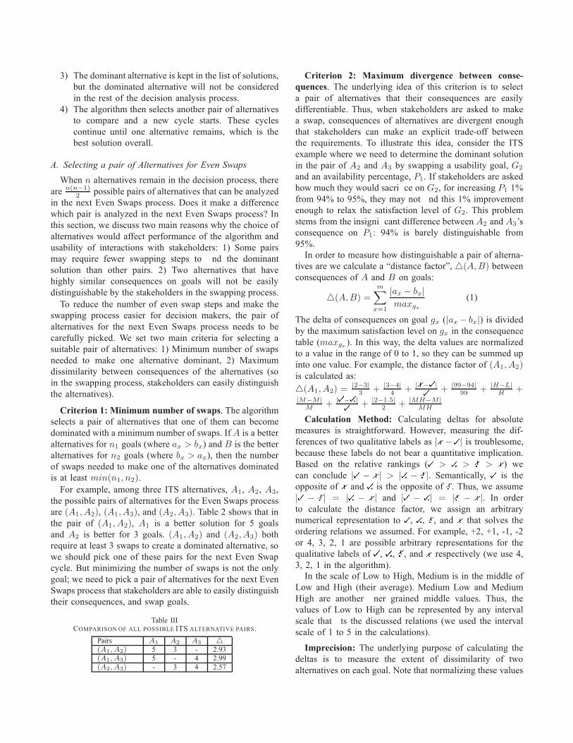
For example, among three ITS alternatives, A1, A2, A3,the possible pairs of alternatives for the Even Swaps processare (A1, A2), (A1, A3), and (A2, A3). Table 2 shows that inthe pair of (A1, A2), A1 is a better solution for 5 goalsand A2 is better for 3 goals. (A1, A2) and (A2, A3) bothrequire at least 3 swaps to create a dominated alternative, sowe should pick one of these pairs for the next Even Swapcycle. But minimizing the number of swaps is not the onlygoal; we need to pick a pair of alternatives for the next EvenSwaps process that stakeholders are able to easily distinguishtheir consequences, and swap goals.

Table IIICOMPARISON OF ALL POSSIBLE ITS ALTERNATIVE PAIRS.

Pairs A1 A2 A3 4(A1, A2) 5 3 - 2.93(A1, A3) 5 - 4 2.99(A2, A3) - 3 4 2.57

Criterion 2: Maximum divergence between conse-quences. The underlying idea of this criterion is to selecta pair of alternatives that their consequences are easilydifferentiable. Thus, when stakeholders are asked to makea swap, consequences of alternatives are divergent enoughthat stakeholders can make an explicit trade-off betweenthe requirements. To illustrate this idea, consider the ITSexample where we need to determine the dominant solutionin the pair of A2 and A3 by swapping a usability goal, G2

and an availability percentage, P1. If stakeholders are askedhow much they would sacri ce on G2, for increasing P1 1%from 94% to 95%, they may not nd this 1% improvementenough to relax the satisfaction level of G2. This problemstems from the insigni cant difference between A2 and A3’sconsequence on P1: 94% is barely distinguishable from95%.

In order to measure how distinguishable a pair of alterna-tives are we calculate a “distance factor”, 4(A, B) betweenconsequences of A and B on goals:

4(A, B) =

m∑

x=1

|ax − bx|

maxgx

(1)

The delta of consequences on goal gx (|ax − bx|) is dividedby the maximum satisfaction level on gx in the consequencetable (maxgx

). In this way, the delta values are normalizedto a value in the range of 0 to 1, so they can be summed upinto one value. For example, the distance factor of (A1, A2)is calculated as:4(A1, A2) = |2−3|

3 + |3−4|4 + | − | + |99−94|

99 + |H−L|H

+|M−M|

M+ | − | + |2−1.5|

2 + |MH−M|MH

Calculation Method: Calculating deltas for absolutemeasures is straightforward. However, measuring the dif-ferences of two qualitative labels as | − | is troublesome,because these labels do not bear a quantitative implication.Based on the relative rankings ( > > > ) wecan conclude | − | > | − |. Semantically, is theopposite of and is the opposite of . Thus, we assume| − | = | − | and | − | = | − |. In orderto calculate the distance factor, we assign an arbitrarynumerical representation to , , , and that solves theordering relations we assumed. For example, +2, +1, -1, -2or 4, 3, 2, 1 are possible arbitrary representations for thequalitative labels of , , , and respectively (we use 4,3, 2, 1 in the algorithm).

In the scale of Low to High, Medium is in the middle ofLow and High (their average). Medium Low and MediumHigh are another ner grained middle values. Thus, thevalues of Low to High can be represented by any intervalscale that ts the discussed relations (we used the intervalscale of 1 to 5 in the calculations).

Imprecision: The underlying purpose of calculating thedeltas is to measure the extent of dissimilarity of twoalternatives on each goal. Note that normalizing these values

does not provide us with means for calculating a meaningfulutility for the alternatives. For example, the percentage ofthe time that cameras are connected (P1) is 95% for A3

(Table I); however, the utility of A3 on P1 is not re ectedby the relation of 95% to the practical maximum connec-tivity percentage (99%) or absolute maximum connectivity(100%). If availability of the connection to cameras is highlycritical, the utility of A2 on P1 is not about 95

99 , and the utilityof any connectivity lower than 99% (for example) could evenbe zero.

With the same argument, one can claim that Formula1 does not measure the dissimilarity of two alternativescorrectly, because if the utility of 95% is zero, the utilityof A2 on P1 (94%) is also zero. Although on the face aredissimilar, A2 and A3 are indifferent with respect to P1.Nevertheless, the distance factors of the pairs of alternativesare comparable because all distance factors are calculatedwith equal imprecision.

For example, 4(A1, A2) =2.93 and 4(A2, A3) =2.57(Table 2), so we conclude that consequences of A1 and A2

are more dissimilar than the consequences of A2 and A3,although both numbers are inaccurate. In the next section,we introduce the automated swap suggestion algorithm toselect the dominant solution in the pair of (A1, A2).

B. Automatically Suggesting SwapsIn each cycle of the algorithm, two alternatives are ana-

lyzed by applying a chain of swaps, until one becomes dom-inated. One of the main goals of the proposed algorithm is toreduce the number of swapping steps through reusing swapsfrom previous cycles. We develop 4 rules for automaticallygenerating reusable swaps that are also easy to make. In thissection, these rules are explained and justi ed.

1) Creating a Dominant Alternative: Swaps make one ofthe decision criteria irrelevant, which helps remove one goalfrom the decision problem in each step. Removing criteriaone by one is a time-consuming approach to apply the EvenSwaps process. For example, consider an alternative suchas A that is dominant for n goals like g1, g2, ... gn, andalternative B that is a better solution only with respect to onegoal, like g. We need to remove g by swapping it with oneof those n goals. By removing g, solution A might still bedominant with respect to all goals (g1, g2, ... gn). However,swapping any two goals from g1, g2, ... gn will not changethe situation between A and B and neither of them becomesdominated with respect to all relevant and remaining goals.By following rule 1, the algorithm suggests a swap that aimsmaking one of the alternatives dominant:

Rule 1, create a dominant alternative: Given a setof goals G = {g1, g2, ...gm}, if consequences of A ={a1, a2, ...am} and consequences of B = {b1, b2, ...bm},and n1 = number of goals where ax > bx and n2 = numberof goals where bx > ax (for 1 ≤ x ≤ m), then n1×n2 swaps

exist that could potentially reduce the number of steps of theEven Swaps process for making an alternative dominant.

For example, between the pair of A1 and A2, with respectto T1, T2, P1, G1, and G3, A1 is a better solution, and withrespect to S1, C1, and C2, A2 is the better solution. Note thatthe satisfaction level of both alternatives on G2 is Medium,so G2 is an irrelevant goal for deciding between A1 and A2.

To minimize the number of swaps for A1 and A2, a goalsuch as gx needs to be swapped with a goal such as gy,where gx ∈ {S1, C1, C2} and gy ∈ {T1, T2, P1, G1, G3}.Therefore, 15 tuples in the form of (gx, gy) exists as thecandidate pair of goals to be swapped. By making a swapbetween such goals, one of three goals among S1, C1, andC2 becomes irrelevant; thus, in the next step, at least 2 moreswaps are needed to make one of the alternatives dominant.

2) Suggesting the Most Reusable Swap: When stakehold-ers make a swap, their value trade-offs can be reused foranother alternative, without further consultation with humanstakeholders (if the goals are the same and the satisfactionlevel of goals in the swap are the same with the newalternative).

Rule 2, pick the most reusable swaps: When thereare several goal tuples like (gx, gy) for the next swap, byapplying rule 2, the algorithm selects the most reusable swapfor the next step. The notion of reusable swap is formallyde ned as follows:

De nition 2. Consider an alternative, A, and goals gx andgy , where A satis es gx and gy at the level of ax and ay .The swap (gx : ix → i′x ⇔ gy : iy → i′y) is reusable foralternative A on goals gx and gy , if ix = ax, and iy = ay .

None of those 15 candidate swaps for A1 and A2 arereusable for the consequences of A3. To illustrate the con-cept of reusability, consider three hypothetical solutions A,B, and C, and three goals g1, g2, and g3, which we aimto maximize. Let us assume consequences of alternatives onthe goals are as:

A = {H, M, L}, B = {MH, L, H}, C = {H, M, ML}

Consider the swap (g1 : H → MH ⇔ g2 : M → x)for deciding between A and B. Assume the stakeholder haspreviously agreed to reduce the satisfaction level of A on g1

from H to MH, and in return, increase the satisfaction levelof g2 from M to x = H . This swap is reusable for decidingbetween B and C as well, where the satisfaction level of C

on g1 and g2 can be modi ed according to this swap withoutthe need for asking another swap from stakeholders.

3) Suggesting Easy Swaps: In addition to consideringswaps reusability, the algorithm suggests swaps that decisionstakeholders would be willing to make. Hammond et al.[13] suggest making the easiest swaps rst, e.g., money isan easy goal to swap. What would make a swap easy forstakeholders? For example, stakeholders may easily agreeto increase improve a goal that is not suf ciently satis ed

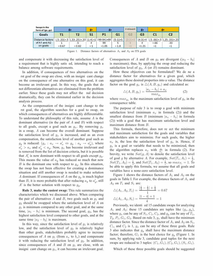
Figure 1. Distance factors of alternatives A1 and A2 on ITS goals

and compensate it with decreasing the satisfaction level ofa requirement that is highly satis ed, intending to reach abalance among software requirements.

In addition, if consequences of two alternatives on the rst goal of the swap are close, with an insigni cant changeon the consequence of one alternative on this goal, it canbecome an irrelevant goal. In this way, the goals that donot differentiate alternatives are eliminated from the problemearlier. Since these goals may not affect the nal decisiondramatically, they can be eliminated earlier in the decisionanalysis process.

As the compensation of the insigni cant change to the rst goal, the algorithm searches for a goal to swap, onwhich consequences of alternatives are highly differentiable.To understand the philosophy of this rule, assume A is thedominant alternative (in the pair of A and B) with respectto all goals, except a goal such as gx. By removing gx

in a swap, A can become the overall dominant. Supposethe satisfaction level of gx is increased, and as an evencompensation, the satisfaction level of another goal such asgy is reduced: (gx : ax → a′

x ⇔ gy : ay → a′y), where

a′x > ax and a′

y < ay. Now, gx has become irrelevant andis removed from the list of decision criteria, but it is possiblethat A′

i is now dominant with respect to all goals except gy.This means the value of ay has reduced so much that nowB is the dominant one with respect to gy . In this situation,the swap has not been effective for creating a dominancesituation and still another swap is needed to make solutionA dominant. If consequences of A on the gy is much higherthan B, it is more probable that after reducing ay to a′

y , stillA′ is the better solution with respect to gy.

Rule 3, make the easiest swap: This rule summarizes thecharacteristics which we discussed above. When comparingthe pair of alternatives A and B, two goals such as g1 andg2 should be swapped where the satisfaction level of A ong1 is minimum compared to any other goal, and at the sametime, |a1 − b1| is minimum. The second goal, g2, has thehighest satisfaction level compared to other goals, and at thesame time |a2 − b2| is maximum.

In this way, since the satisfaction level of g1 is relativelylow, and the satisfaction level of g2 is relatively higherthan other goals, stakeholders probably agree to increaseconsequences of A on g1 (from ax to bx) and compensateit with reducing the satisfaction level of g2. In addition,since consequences of A and B on g1 are close, with aninsigni cant change on g1, it can become an irrelevant goal.

Consequences of A and B on g2 are divergent (|a2 − b2|is maximum); thus, by applying the swap and reducing thesatisfaction level of g2, A (or B) remains dominant.

How these objectives can be formulated? We de ne adistance factor for alternatives for a given goal, whichaggregates these desired properties into a value. The distancefactor on the goal gx is 4(A, B, gx) and calculated as:

4(A, B, gx) =|ax − bx| + ax

maxgx

(2)

where maxgxis the maximum satisfaction level of gx in the

consequence table.The purpose of rule 3 is to swap a goal with minimum

satisfaction level (minimum ax in formula (2)) and thesmallest distance from B (minimum |ax − bx| in formula(2)) with a goal that has maximum satisfaction level andmaximum distance from B.

This formula, therefore, does not re ect the minimumand maximum satisfaction for the goals and variables thatstakeholders aim to minimize. For such goals, the higherax is, the less the satisfaction level of gx is. Hence, ifgx is a goal or variable that needs to be minimized, thenthe algorithm replaces ax with 1

ax

in formula (2). Forbrevity, we write Sat(g, A) to denote the satisfaction levelof goal g by alternative A. For example, Sat(T1, A1) = 1

2 ,Sat(T1, A2) = 1

3 , and Sat(T1, A3) = 11 , so maxT1

= 1. Tobe able to apply this formula, we assume that all goals andvariables have a none-zero satisfaction level.

Figure 1 shows the distance factors of A1 and A2 on thegoals in Table I. For example, the distance factors of A1 andA2 on T1 and S1 are:

4(A1, A2, T1) =| 12 − 1

3 | +12

1= 0.67

4(A1, A2, S1) =|1 − 4| + 1

4= 1

Previously, we identi ed 15 candidate swaps for analyzingA1 and A2: these 15 candidates are tuples like (gx, gy),where gx can be any of S1, C1, C2, and gy can be any of T1,T2, P1, G1, G3. Based on rule 3, gx shall have the minimumdistance factor. Since the distance factor of A1 and A2 on S1,C1, and C2 is 1, gx can be any of these three goals. Rule3 also indicates that gy shall have the maximum distancefactor; therefore, G1 is the best choice for gy (Figure 1. Insum, by applying rule 3, candidate goal tuples for the nextswaps are reduced to 3 tuples: (C1, G1), (C2, G1), (S1, G1).

Which of these three possible goals should be suggested

for the next swap? The nal rule for suggesting the nextswap is selecting goals that are measured in more granularand accurate scales, because dealing with tangible factorsis easier for stakeholders. For example, costs in terms ofmoney is more tangible than the usability level expressed asMedium, Low, High. In this regard, rule 4 states:

Rule 4, pick preferred scales: Goals that are measuredin absolute values are preferred to the goals measured inpercentages, percentages are preferred to ordinal values, andthe least preferred scale is qualitative labels.

For example, based on rule 4, the scale of C2 is preferredto the scale of S1 and the scale of C1 is preferred to C2, sinceC1 is an absolute value (million dollars). Therefore, amongthree options ((C1, G1), (C2, G1), (S1, G1)), the algorithmselects C1 and G1 to be swapped, and asks the value of x

in the swap: (C1 : $ 2m → $1.5m ⇔ G1 : H → x).The aim of this swap is to elicit how much stakeholders

would give up on G1 for paying a lower price (C1), so C1

is reduced to from $2m to $1.5m, and as a compensation,G1 is decreased from H to a lower level (x). Suppose thestakeholder agrees with x = L. The consequence table isrevised with these new values (the satisfaction level of G1

under the consequence of A1 is now L, and the cost ofalternative A1 is now $1.5 million). C1 can be removedfrom the list of goals that need to be considered for decidingbetween A1 and A2. (Not deliberately, the swap makes G1

irrelevant as well.)4) Reusing Dominance Situations: Once an alternative is

decided as the dominant one in a pair, this knowledge canbe reusable for deciding between other pairs of alternativeswithout the need to the even swaps process. For example,consider four hypothetical solutions A, B, C, and D andthree goals g1, g2, and g3, where consequences of alterna-tives on the goals are as:

A = {H, M, L} , B = {MH, L, H}C = {H,M, ML}, D = {M, L, H}

Assume by applying a chain of swaps, the algorithm con-cludes that A > B, then we can conclude that C > D

as well, because C dominates A on every goal, and B

dominates D on every goal. Since dominance is a transitiverelation, we can conclude that C dominates D:

Reuse the dominance situation: In general, for fouralternatives A, B, C, and D, where the consequencesof alternatives on goals G = {g1, g2, ..., gm}, A ={a1, a2, ..., am}, B = {b1, b2, ...bm}, C = {c1, c2, ..cm},and D = {d1, d2, ...dm}. If A > B, then C > D too, iff:

- ∀(ax, cx) cx ≥ ax

- ∀(bx, dx) dx ≤ bx

(1 ≤ x ≤ m)

C. The Automated Swaps Suggestion AlgorithmAssume a consequence table that includes a set of goals

G = {g1, g2, ...gm}, and two alternatives A and B to beanalyzed in the next cycle of the algorithm. The algorithm

suggests swaps, gets the stakeholders input, applied theswap, and stores the swaps in a Knowledge Base (KB). Ineach step, the algorithm keeps the tuples of candidate goalsfor the next swap in temporary array lists of L, L′, L′′, Lf .The process for determining the optimum solution betweenA and B consists of 8 main steps as follows.While NOT(A is dominant OR B is dominant)

Step 1: Remove irrelevant goalsFor all gx in G:

If ax = bx Then remove gx, ax, bx from G, A, B

Step 2: Reuse swapsFor all swap In SwapsKB

If swap is reusable to A OR B ThenApply swapRepeat Step 1: Remove irrelevant goals

Step 3: Apply Rule 1, create a dominance situationFor x = 1 To m

If ax > ay AND bx > by Then L.add((gx, gy))Step 4: Apply rule 2, nd the most reusable swaps

For all (gx, gy) in LL′.add(the most reusable (gx, gy))

If NOT exist a reusable (gx, gy) in L Then L′ = L

Step 5: Apply rule 3, make the easiest swapsFor all gx in G (1 ≤ x ≤ m)

If gx.Target = MINIMIZE ThenFor all Alternatives Ai in Consequence Table

Sat(gx, Ai) = 1

ax

For all (gx, gy) in L′

If |ax−bx|+ax

maxgx

is Min AND|ay−by|+ay

maxgy

is Max Then

L′′.add((gx, gy))Step 6: Apply rule 4, select the preferred scales

For all (gx, gy) in L′′

If gx and gy have the most preferred scalesThen Lf .add((gx, gy))

Step 7: Ask the swap from stakeholders(gx, gy) = random tuple in Lf

Ask value of a′y in swap (gx : ax → bx ⇔ gy : ay → a′

y)Sat(gx, A)=bx

Sat(gy , A)=a′y

SwapsKB.add(gx : ax → bx ⇔ gy : ay → a′y)

End While

If A is dominant OR B is dominantStep 8: Reuse the dominance situation

For all Alternatives Ax, Ay in Consequence TableIf A, B dominance is reusable in Ax, Ay Then

Apply the dominance to Ax, Ay

V. CASE STUDIES AND COMPARISON

We illustrate the use of the proposed method by ana-lyzing a number of case studies including the alternativeITS systems. We focus on evaluating three characteristicsof the method: 1) number of swap enquiries asked fromstakeholders to determine the dominant alternative 2) theinitial data needed to make the decision 3) validity of thedecision made by the algorithm.

Case study 1: alternative ITS systems at MTO. In theprevious section, we explained how the algorithm selectsthe pair of A1 and A2 for the rst Even Swaps process.First, the algorithm suggests and applies (C1 : $ 2m →$1.5m ⇔ G1 : H → L). C1 and G1 become irrelevant,

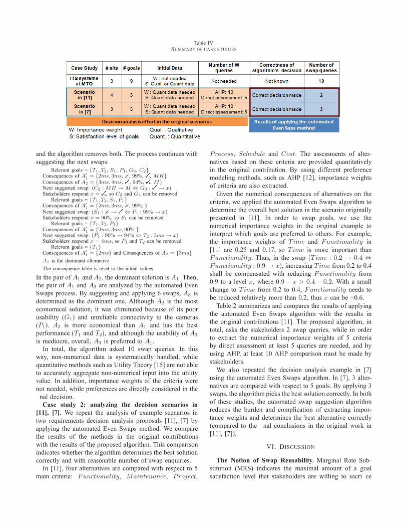
Table IVSUMMARY OF CASE STUDIES

and the algorithm removes both. The process continues withsuggesting the next swaps:

Relevant goals = {T1, T2, S1, P1, G3, C2}Consequences of A′

1= {2ms, 3ms, , 99%, , MH}

Consequences of A2 = {3ms, 4ms, , 94%, , M}Next suggested swap: (C2 : MH → M ⇔ G3 : → x)Stakeholders respond x = , so C2 and G3 can be removed

Relevant goals = {T1, T2, S1, P1}Consequences of A′

1= {2ms, 3ms, , 99%, }

Next suggested swap: (S1 : → ⇔ P1 : 99% → x)Stakeholders respond x = 90%, so S1 can be removed

Relevant goals = {T1, T2, P1}Consequences of A′

1= {2ms, 3ms, 90% }

Next suggested swap: (P1 : 90% → 94% ⇔ T2 : 3ms → x)Stakeholders respond x = 4ms, so P1 and T2 can be removed

Relevant goals = {T1}Consequences of A′

1= {2ms} and Consequences of A2 = {3ms}

A1 is the dominant alternativeThe consequence table is reset to the initial values

In the pair of A1 and A2, the dominant solution is A1. Then,the pair of A1 and A3 are analyzed by the automated EvenSwaps process. By suggesting and applying 6 swaps, A3 isdetermined as the dominant one. Although A2 is the mosteconomical solution, it was eliminated because of its poorusability (G1) and unreliable connectivity to the cameras(P1). A3 is more economical than A1 and has the bestperformance (T1 and T2), and although the usability of A3

is mediocre, overall, A3 is preferred to A1.In total, the algorithm asked 10 swap queries. In this

way, non-numerical data is systematically handled, whilequantitative methods such as Utility Theory [15] are not ableto accurately aggregate non-numerical input into the utilityvalue. In addition, importance weights of the criteria werenot needed, while preferences are directly considered in the nal decision.

Case study 2: analyzing the decision scenarios in[11], [7]. We repeat the analysis of example scenarios intwo requirements decision analysis proposals [11], [7] byapplying the automated Even Swaps method. We comparethe results of the methods in the original contributionswith the results of the proposed algorithm. This comparisonindicates whether the algorithm determines the best solutioncorrectly and with reasonable number of swap enquiries.

In [11], four alternatives are compared with respect to 5main criteria: Functionality, Maintenance, Project,

Process, Schedule and Cost. The assessments of alter-natives based on these criteria are provided quantitativelyin the original contribution. By using different preferencemodeling methods, such as AHP [12], importance weightsof criteria are also extracted.

Given the numerical consequences of alternatives on thecriteria, we applied the automated Even Swaps algorithm todetermine the overall best solution in the scenario originallypresented in [11]. In order to swap goals, we use thenumerical importance weights in the original example tointerpret which goals are preferred to others. For example,the importance weights of T ime and Functionality in[11] are 0.25 and 0.17, so T ime is more important thanFunctionality. Thus, in the swap (T ime : 0.2 → 0.4 ⇔Functionality : 0.9 → x), increasing T ime from 0.2 to 0.4shall be compensated with reducing Functionality from0.9 to a level x, where 0.9 − x > 0.4 − 0.2. With a smallchange to T ime from 0.2 to 0.4, Functionality needs tobe reduced relatively more than 0.2, thus x can be =0.6.

Table 2 summarizes and compares the results of applyingthe automated Even Swaps algorithm with the results inthe original contributions [11]. The proposed algorithm, intotal, asks the stakeholders 2 swap queries, while in orderto extract the numerical importance weights of 5 criteriaby direct assessment at least 5 queries are needed, and byusing AHP, at least 10 AHP comparison must be made bystakeholders.

We also repeated the decision analysis example in [7]using the automated Even Swaps algorithm. In [7], 3 alter-natives are compared with respect to 5 goals. By applying 3swaps, the algorithm picks the best solution correctly. In bothof these studies, the automated swap suggestion algorithmreduces the burden and complication of extracting impor-tance weights and determines the best alternative correctly(compared to the nal conclusions in the original work in[11], [7]).

VI. DISCUSSION

The Notion of Swap Reusability. Marginal Rate Sub-stitution (MRS) indicates the maximal amount of a goalsatisfaction level that stakeholders are willing to sacri ce

for a unit of increase in another goal. Even swaps implicitlycapture the MRSs for the goals that stakeholders swap.Generally, MRSs of two goals at two different satisfactionlevels can be different [16]. The notion of swaps reusabilitywhich we discussed in the previous section is based onassuming that MRSs are static, and the consequence changesmade in an even swap depend on the satisfaction levels of thegoals; this restricts the reusability of swaps. In what follows,we explain the underlying reasons for assuming that MRSsare static.

In the swap (gx : ix → i′x ⇔ gy : iy → i′y), changing gx

by dx levels (dx = |i′x − ix|) is compensated with changinggy by dy levels (dy = |iy − i′y|). Here, stakeholders havea mental utility function like F, which helps them balance|F (i′x) − F (ix)| with |F (iy) − F (i′y)|. However, the utilityfunction, F , is not linear; hence, in a situation where thesatisfaction level of gx is not equal to ix, changing gx

by dx levels cannot be compensated with changing gy bydy levels. F is not linear because people have different“mental” spending accounts for different goals [17], i.e., if astakeholder reaches the maximum amount that is willing tospend on satisfying a goal gx, he/she will not sacri ce othergoals for gx, if gx is already highly satis ed. Even thoughstakeholders may have previously increased the satisfactionlevel of gx and compensated it by decreasing other goals,but as soon as they psychologically feel that too much isspent on gx, the MRS they are willing to spend on gx wouldchange in the next Even Swaps queries.

For example, if stakeholders previously made a swapas (T1 : 3ms → 2ms ⇔ C1 : $1.9m → $2m), itdoes not indicate that whenever T1 is reduced 1 ms, then,stakeholders are willing to pay an extra $0.1 m. For instance,if humans cannot sense the difference between the 2 msand 1 ms delays, reducing T1 to less than 2 ms does notprovide any extra value on performance. Therefore, the swap(T1 : 2ms → 1ms ⇔ C1 : $1.9m → $2m) is not valid andreusable. This limits the reusability of swaps and increasesthe number of swap queries needed.

Method Feasibility. Making trade-offs by even swapsmay need substantial cognitive abilities and domain knowl-edge. If stakeholders are not able to swap suggested goals,the tool suggests the next best swap, and stores the rejectedswap in a “black list”, and in the rest of the process, wouldnot ask that swap from the stakeholder. In practice, stake-holders may reject every suggested swap, which results inseveral tedious swap queries to nd the one that stakeholderis able to answer. The process may become time-consumingor never ends.

To prevent the dead-ends, after a number of rejectedsuggestions, the tool asks the users to select the goals for thenext swap themselves. Nevertheless, if stakeholders are notable the specify the maximal amount of a goal satisfactionlevel that they are willing to sacri ce for a unit of increase

in another goal, then it is probable that they will not be ableto numerically specify preferences over the goals either.

We have also assumed that stakeholders would makeconsistent swaps among goals. In practice, however, stake-holders are not always consistent in their judgements. Asfuture work, we intend to enhance our tool to trace theinconsistencies in even swaps.

Another threat to practicality of the algorithm is thediversity of evaluation scales in the consequence table.Stakeholders may not be able to swap a goal measured inabsolute values with a goal that is evaluated by qualitativelabels such as and . In future work, we intend to conductempirical experiments to examine which types of swaps areeasy/hard to make.

VII. RELATED WORK

Multi-Criteria Decision Analysis (MCDA) methods havebeen successfully applied in the elds of economics, opera-tion research, and management science, and can potentiallybe used in RE for deciding on alternative solutions tosatisfy requirements. For example, requirements decisionmethods, such as [1], [7], [18], [8], [9], [10], rely on theavailability, accuracy, and meaningfulness of quantitativecosts and bene ts measures for making decisions.

Feather et al. [1] propose a quantitative model for strategicdecision analysis and trade-off analysis considering qualityrequirements, by the “coarse quanti cation” of relevant riskfactors and their interactions. Letier and Lamsweerde [10]argue that due to the lack of accuracy and measurabilityof goal formulations and lack of impact propagation rulesthrough goal models, domain-speci c quality variables areneeded to reason on partial goal satisfaction.

Utility values are used for representing quality value ofNFRs in [19]. In the Utility Theory (Keeney and Raiffa[15]) the quantitative preference and measures are conjointlyused to calculate the total utility value for each alternative.Preference (utility) elicitation involves a sequence of queriesand interactions with the decisions stakeholders to obtainenough information about individual preferences. AHP [12]is a theory of relative measurement of intangible criteriato derive a numerical scale of priorities (preferences, im-portance weights) from pairwise comparisons of elements.Karlsson et al. [18] apply AHP for prioritizing softwarerequirements and a cost-value analysis. A case study ofapplying AHP for software requirements prioritizing is givenby Karlsson in [20].

The Even Swaps [13] method avoids eliciting explicitnumerical priorities, and yet incorporates the stakeholders’preferences in determining the optimum solution by query-ing value trade-offs between stakeholders’ goals.

The need for automated tool support for suggesting swapsto decision analysts has been recognized [21], [14]. In [21],consequence changes made in an even swap are not assumedto depend on the satisfaction levels of the goals, which

allows using the trade-off information given in an even swapto represent the stakeholders’ general preferences over thegoals. The Smart Swaps tool [14] suggests next swaps to theuser based on preference programming assumptions madein [21]. The Smart Swaps tool navigates the swap chainstoward 1) making goals irrelevant and 2) making alternativesone step closer to the dominance situation.

In the current work, in addition to those two goals, weintroduce other criteria for suggesting the next swaps, suchas reusability of swaps, swaps that are cognitively easy tomake, preferring numerical scales to qualitative ones, etc.Our tool is tailored for requirements trade-off analysis, e.g.,the tool suggests swaps that stakeholders are willing to makeamong requirements with minimal sacri ce to be made onrequirements. A demo of the proposed tool in this paper isavailable at [22].

The algorithm in the current work is developed basedon the opposite assumption made in [21], i.e., we assumethat consequence changes made in an even swap do notrepresent stakeholders’ general preferences. In Section VI,we justi ed this assumption and explained its implication onthe proposed algorithm.

VIII. CONCLUSIONS

In this work, we adopt and enhance the Even Swaps[13] method for analyzing trade-offs among requirementswhen multiple alternative design solutions satisfy differentrequirements to some extent. The main contribution of thispaper is proposing a set of rules for suggesting next swaps tothe decision stakeholders. The algorithm and prototype toolhandle different types of input data: absolute and ordinalvalues in different scales.

ACKNOWLEDGMENTFinancial support from the Natural Sciences and Engineering

Research Council of Canada is gratefully acknowledged. Authorsthank Jocelyn Simmonds and Jennifer Horkoff for insightful com-ments on this work. We would like to thank ONE-ITS projectmembers specially Roger Browne at Ministry of Transportation,Ontario (MTO), Professor Tamer El-Diraby and Mahmoud OsmanAbou-Beih.

REFERENCES

[1] M. S. Feather, S. L. Cornford, K. A. Hicks, J. D. Kiper, andT. Menzies, “A broad, quantitative model for making earlyrequirements decisions,” IEEE Software, vol. 25, pp. 49–56,2008.

[2] E. Yu, “Modeling Strategic Relationships for Process Reengi-neering,” Ph.D. dissertation, University of Toronto, 1995.

[3] P. Giorgini, J. Mylopoulos, E. Nicchiarelli, and R. Sebastiani,“Formal reasoning techniques for goal models,” Journal ofData Semantics, vol. 1, pp. 1–20, 2003.

[4] L. Chung, B. A. Nixon, E. Yu, and J. Mylopoulos, Non-Functional Requirements in Software Engineering. KluwerAcademic, 1999.

[5] J. Horkoff and E. Yu, “A Qualitative, Interactive EvaluationProcedure for Goal- and Agent-Oriented Models,” in CAiSEForum, 2009.

[6] P. Giorgini, J. Mylopoulos, and R. Sebastiani, “Goal-orientedrequirements analysis and reasoning in the tropos methodol-ogy,” Eng. Appl. Artif. Intell., vol. 18, no. 2, pp. 159–171,2005.

[7] W. Ma, L. Liu, H. Xie, H. Zhang, and J. Yin, “Preferencemodel driven services selection,” in Proc. of CAiSE’09, 2009,pp. 216–230.

[8] P. Giorgini, G. Manson, and H. Mouratidis, “On security re-quirements analysis for multi-agent systems.” in SELMAS’03,2003.

[9] Y. Asnar and P. Giorgini, “Modelling risk and identifyingcountermeasure in organizations,” 2006, pp. 55–66.

[10] E. Letier and A. van Lamsweerde, “Reasoning about partialgoal satisfaction for requirements and design engineering,” inSIGSOFT ’04/FSE-12, 2004, pp. 53–62.

[11] H. P. In, D. Olson, and T. Rodgers, “Multi-criteria preferenceanalysis for systematic requirements negotiation,” in Proc. ofthe COMPSAC’02, ser. COMPSAC ’02, 2002, pp. 887–892.

[12] T. Saaty, The Analytic Hierarchy Process, Planning, PioritySetting, Resource Allocation. New york: McGraw-Hill, 1980.

[13] J. S. Hammond, R. L. Keeney, and H. Raiffa, Smart choices :a practical guide to making better life decisions. BroadwayBooks, 2002.

[14] J. Mustajoki and R. P. Hamalainen, “Smart-swaps - a decisionsupport system for multicriteria decision analysis with theeven swaps method,” Decis. Support Syst., vol. 44, no. 1, pp.313–325, 2007.

[15] R. L. Keeney and H. Raiffa, Decisions with multiple objec-tives : preferences and value tradeoffs. Wiley, 1976.

[16] J. Yen and W. A. Tiao, “A systematic tradeoff analysis forcon icting imprecise requirements,” in RE ’97, 1997, p. 87.

[17] B. Schneier, “The psychology of security,” Commun. ACM,vol. 50, no. 5, p. 128, 2007.

[18] J. Karlsson and K. Ryan, “A cost-value approach for priori-tizing requirements,” IEEE Softw., vol. 14, no. 5, pp. 67–74,1997.

[19] H. Xie, L. Liu, and J. Yang, “i*-prefer: optimizing require-ments elicitation process based on actor preferences,” in SAC’09: Proceedings of the 2009 ACM symposium on AppliedComputing, 2009, pp. 347–354.

[20] J. Karlsson, “Software requirements prioritizing,” In 2ndIEEE International Conference on Requirements Engineering,pp. 100–116, 1996.

[21] J. Mustajoki and R. P. Hamalainen, “A preference program-ming approach to make the even swaps method even easier,”Decision Analysis, vol. 2, no. 2, pp. 110–123, 2005.

[22] (2011) Decision analysis tool demo, release 1, dcs, univ. oftoronto, available at http://www.cs.toronto.edu/ gelahi/Release1/Release1.html.