A Semi-Analytical Method for Calculating Revisit Time for Satellite Constellationswith Discontinuous Coverage

Nicholas H. Crispa,∗, Sabrina Livadiottia, Peter C.E. Robertsa

aSchool of Mechanical, Aerospace and Civil Engineering, The University of Manchester, George Begg Building, Sackville St, Manchester,M13 9PL

Abstract

This paper presents a unique approach to the problem of calculating revisit time metrics for different satellite orbits,sensor geometries, and constellation configurations with application to early lifecycle design and optimisation processesfor Earth observation missions. The developed semi-analytical approach uses an elliptical projected footprint geometryto provide an accuracy similar to that of industry standard numerical orbit simulation software but with an efficiencyof published analytical methods. Using the developed method, extensive plots of maximum revisit time are presentedfor varying altitude, inclination, target latitudes, sensor capabilities, and constellation configuration, providing valuablereference for Earth observation system design.

Keywords: Revisit time; satellite constellation; discontinuous satellite coverage; Earth observation.

1. Introduction

During the design of Low Earth Orbit (LEO) systemsof satellites performance metrics are required to evaluatedifferent orbital configurations and payload specifications.For Earth observation or communications missions the ex-tent of coverage of the system or rate at which the systemvisits or views different locations is of particular interestto the mission designer. Revisit time (also known as theresponse time or coverage gap) is often used as a key per-formance metric for LEO systems which do not have con-tinuous coverage of an area of interest and is defined as theduration in time between consecutive viewings of a givenlocation on the Earth. Most commonly, the Maximum Re-visit Time (MRT) and Average Revisit Time (ART) overa given target area and period of analysis are consideredduring the mission design process.

With increasing on-orbit capability and reduced sys-tem cost, development of constellations of small satelliteshas recently grown significantly. However, the design andoptimisation of these systems is complex and multidisci-plinary, owing to the number of different design variablesand ranges which they can take. For example, consider-ation of the orbit design, system configuration, payloadcharacteristics, and mission performance can all have a

∗Corresponding author.Email addresses: nicholas.crisp@manchester.ac.uk

(Nicholas H. Crisp),sabrina.livadiotti@postgrad.manchester.ac.uk

(Sabrina Livadiotti), peter.c.e.roberts@manchester.ac.uk(Peter C.E. Roberts)

significant effect on the final system utility and cost. Foran Earth observation satellite or constellation the evalua-tion of revisit time therefore forms a critical component ofthe design and optimisation process.

Often the analysis of coverage or revisit metrics forsatellites and constellations is performed using commer-cially available orbital propagation and simulation soft-ware such as STK (Systems Tool Kit) [1, 2, 3]. However,due to the numerical nature of these programs and po-tential for long analysis periods (on the order of minutes)or large numbers of satellites, the computational time canbecome considerable. Furthermore, when many cases areto be considered, for example within a wider frameworkfor system optimisation, a faster, open, and stand-alonemethod is preferred.

A number of methods for calculating revisit time havebeen discussed and applied in the literature. Wertz [4, 5]provides basic descriptions for evaluating coverage usingsimple analytical expressions and calculating revisit met-rics using two numerical treatments. The first, a numericalmethod, utilises simple ground track plots and mission ge-ometry and is shown to be most useful for rapid missionanalysis. The second, point coverage simulation methods,use a grid of points at which visibility characteristics arebe evaluated. These methods are able to provide insightinto the statistical measures of coverage and can achievegreater accuracy albeit at the cost of longer computationtimes.

Bottkol and DiDomenico [6] describe a numerical phase-based approach to the calculation of revisit interval. Inthis method the satellite ground track is mapped to thesurface of a torus which is then unwrapped to indicate theintersection with a defined visibility region. The devel-

Preprint submitted to arXiV cs.CE July 6, 2018

arX

iv:1

807.

0202

1v1

[cs

.CE

] 5

Jul

201

8

Nomenclature

∆λ Ground track shift

δΩ Regression rate of RAAN

ε Elevation angle

γ Intermediate angle

Λ Half surface dihedral angle of sensor

λ Longitude

µE Earth gravitational parameter

ν True anomaly

Ω Right Ascension of Ascending Node (RAAN)

ω Argument of perigee

ωE Earth rotation rate

φ Target latitude

ψ Sensor boresight half cone angle

ρ Slant range

θ Half ground range angle of sensor

a Semi-major axis

e Eccentricity

h Altitude

i Inclination

J2 Second-degree Earth zonal harmonic

n Mean motion

p Semilatus Rectum

Pk Keplerian period

Pn Nodal period

R Earth radius

Ra Earth equatorial radius

Rb Earth polar radius

rs Orbital radius

oped method is subsequently used to perform the designof satellite constellations for optimal coverage and revisitcharacteristics. However, the analysis is limited to orbitswhich have a short repeating ground track period and cantherefore not address the complete range of low Earth or-bits.

Ulybyshev [7, 8] presents a geometric analysis methodfor the calculation of revisit time. Reasonable agreementon the order of 2% error in maximum revisit time is shownwith STK for a limited number of cases. Razoumny [9] alsopresents a general analytical method for the problem ofdiscontinuous coverage. However, for these methods onlylimited validation is provided and computational perfor-mance is not given explicitly.

The design of satellite constellations for optimal re-visit metrics has been studied extensively in the literature.Lang and Hanson [10] first worked towards minimization ofMRT by considering variable orbital inclination and con-stellation configuration. Lang [11] later applied a geneticalgorithm optimisation process to this problem enabling aparametric exploration of the design space. Crossley andWilliams [12] similarly investigated the use of genetic al-gorithm and simulated annealing approaches to minimisa-tion of MRT of satellite constellations. Further investiga-tions of satellite constellation optimisation for revisit andcoverage metrics are performed by Ferringer and Spencer[13], Ferringer et al. [14]. However, in each of these stud-ies the analysis of revisit time is performed using the pro-prietary COVERIT and ASTROLIB/Revisit-C programsof The Aerospace Corporation. These tools utilise a nu-merical point coverage simulation method and generated

ephemeris tables for the satellites to calculate revisit time.A representative computation time of 0.5 s per functioncall is given by Ferringer and Spencer [13] on an Intel Pen-tium III 1200 MHz processor.

Abdelkhalik and Mortari [15] address the design of op-timal satellite orbits for the surveillance of multiple targetsites. The method utilises propagated satellite orbits overa short time period and a penalty function method to de-sign satellite orbits for maximum resolution or maximumobservation time. Abdelkhalik and Gad [16] subsequentlyperform the design of optimal repeat ground track sun-synchronous orbits for multiple site surveillance by consid-ering the intersection of the J2-perturbed rotating orbitalplane with the target sites.

Given the noted interest in extensive trade-studies formulti-satellite systems and constellations, using large-scaledesign optimisation or Monte Carlo processes, a meansto efficiently calculate orbital revisit metrics is necessary.Furthermore, the solution of observation characteristics fornumerous orbital conditions can be beneficial for VLEOand CubeSat or nano-class missions which may consist ofmany payloads operating at low orbital altitudes and sub-ject to free or controlled decay.

The method presented herein offers an accurate and ef-ficient analytical calculation process for revisit metrics ofindividual satellites or constellations with discontinuouscoverage of a given target observation area. Considerationof the oblate spheroid approximation for the Earth and as-sociated orbital perturbation is included. The method isdemonstrated to be capable of rapidly calculating orbitalrevisit time with an accuracy on the order of commer-

2

cial numerical simulation software. Finally, revisit charac-teristics for different target latitudes, orbital parameters,sensor characteristics, and constellation configurations areexplored.

2. Calculation of Maximum Revisit Time

Calculation of the revisit time at a given latitude canbe determined by correlating the longitude of all projectedpasses and the instantaneous coverage of the sensor over aperiod of analysis. The maximum time gap between anytwo continuous passes (ordered by time) at any longitudegives the simple MRT. Similarly, ART can be calculated.Contrastingly, the time to 100% coverage can be deter-mined when the maximum difference in longitude betweenany two contiguous passes (ordered by longitude) falls be-low the angular range of the sensor.

To maintain the accuracy of this method for low incli-nation orbits and at increasing latitudes of interest con-sideration must be given to rotation of the Earth duringeach pass and the angle of the orbit track with respect tothe latitude of interest. These effects can provide sensoraccess to longitudes which are beyond the simple sensorwidth at the point where the orbit intercepts the latitudeof interest. These passes can be examined by consideringthe ground track of the orbit in the vicinity of the latitudecrossing and by idealising the sensor coverage area as anellipse.

2.1. Simple Orbit and Sensor Geometry

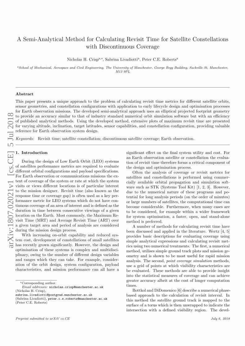
The calculation of maximum revisit time first requiresa treatment of the orbit geometry and Field of Regard ofthe sensor, shown in Fig. 1, to yield the half ground rangeangle θ visible to the satellite. Alternatively, a minimumelevation angle ε constraint can be applied to specify thesensor geometry and half ground range angle θ.

First, the geodetic radius Rφ is calculated at the targetlatitude φ. Here, the Earth is assumed to be an oblatespheroid where Ra and Rb are the equatorial and polarradii respectively.

R (φ) =

√(R2

a cosφ)2

+ (R2b sinφ)

2

(Ra cosφ)2

+ (Rb sinφ)2 (1)

The height hφ and radius of the satellite rs at nadir can befound by considering the semi-major axis a, eccentricity e,argument of perigee ω, and true anomaly νφ at the targetlatitude.

νφ = sin−1

sinφ

sin i

− ω (2)

rs = Rφ + hφ =p

1 + e cos νφ(3)

where the semilatus rectum p is defined as

p = a(1− e2)

From a given elevation angle constraint ε, the half groundrange angle θ can be calculated by considering the obliquetriangle OSP.

θ = cos−1

(Rφrs

cos ε

)− ε (4)

Alternatively, given the angular field of regard or half-coneboresight angle ψ available to the sensor an intermediateangle γ and the slant range ρ to the edge of the sensorcoverage area can first be calculated.

sin γ = sin(ε+ π

2

)=

(rs sinψ

Rφ

)(5)

ρ = Rφ cos γ + rs cosψ (6)

The half ground range angle θ from the nadir can then becalculated using the sine-law.

sin θ =ρ sinψ

Rφ(7)

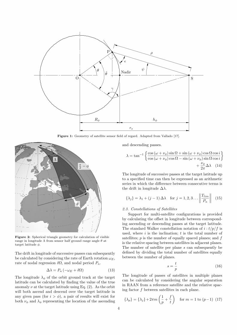
The surface dihedral angle Λ, analogous to the coveragein longitude of the sensor at the target latitude, is cal-culated from the ground range angle using the sphericaltrigonometry shown Fig. 2.

cos θ = cos(π2 − φ) cos(π2 − φ)

+ sin(π2 − φ) sin(π2 − φ) cos Λ (8)

Λφ = 2Λφ = 2 cos−1

(cos θ − sin2 φ

cos2 φ

)(9)

2.2. Calculation of Longitude of Successive PassesIn order to find the maximum difference in time be-

tween any two passes over the same point, the crossinglongitudes of the satellite(s) at the target latitude is re-quired. A J2 perturbed orbit is assumed to include therotation of the orbital plane due to the non-spherical po-tential of the Earth. First, the the nodal period Pn of theorbit is calculated from the Keplerian period Pk [17].

Pk = 2π

√a3

µE(10)

Pn = Pk

[1 +

3J2Ra4p

√1− e2

(2− 3 sin2 i

)+(4− 5 sin2 i

)]−1

(11)

Then drift in Right Ascension of Ascending Node (RAAN)due to J2 orbit regression is also calculated [17]. Extendedexpressions for the secular effect on RAAN by further zonalharmonics (J4, J6) can also be used.

δΩ =− 3

2nJ2

(Rap

)2

cos i

+3

32nJ2

2

(Rap

)4

cos i[12− 4e2 −

(80 + 5e2

)sin2 i

](12)

3

ψ

γ

θθ

ρ

Rφ hφ

rs

Nadir

S

P

O

ε

Figure 1: Geometry of satellite sensor field of regard. Adapted from Vallado [17].

θ

π2 − φ

Λ

Figure 2: Spherical triangle geometry for calculation of visiblerange in longitude Λ from sensor half ground range angle θ attarget latitude φ.

The drift in longitude of successive passes can subsequentlybe calculated by considering the rate of Earth rotation ωE ,rate of nodal regression δΩ, and nodal period Pn.

∆λ = Pn (−ωE + δΩ) (13)

The longitude λφ of the orbit ground track at the targetlatitude can be calculated by finding the value of the trueanomaly ν at the target latitude using Eq. (2). As the orbitwill both ascend and descend over the target latitude inany given pass (for i > φ), a pair of results will exist forboth νφ and λφ representing the location of the ascending

and descending passes.

λ = tan−1

cos (ω + νφ) sin Ω + sin (ω + νφ) cos Ω cos i

cos (ω + νφ) cos Ω− sin (ω + νφ) sin Ω cos i

+νφ2π

∆λ (14)

The longitude of successive passes at the target latitude upto a specified time can then be expressed as an arithmeticseries in which the difference between consecutive terms isthe drift in longitude ∆λ.

λj = λ1 + (j − 1) ∆λ for j = 1, 2, 3 . . .

∥∥∥∥TlimPn∥∥∥∥ (15)

2.3. Constellations of Satellites

Support for multi-satellite configurations is providedby calculating the offset in longitude between correspond-ing ascending or descending passes at the target latitude.The standard Walker constellation notation of i : t/p/f isused, where i is the inclination; t is the total number ofsatellites; p is the number of equally spaced planes; and fis the relative spacing between satellites in adjacent planes.The number of satellite per plane s can subsequently bedefined by dividing the total number of satellites equallybetween the number of planes.

s =t

p(16)

The longitude of passes of satellites in multiple planescan be calculated by considering the angular separationin RAAN from a reference satellite and the relative spac-ing factor f between satellites in each plane.

λp = λj+2πm

(1

p+f

t

)for m = 1 to (p−1) (17)

4

φ

Πφν

λν

Λ

θ

OrbitTrack

O

(φ, λφ)

Figure 3: Reference geometry used to determine whether a givenpoint at the target latitude exists within the boundary of therepresentative sensor ground ellipse.

Similarly, the longitude of corresponding passes of multiplesatellites in a each plane can be calculated by consideringthe in-track spacing between the satellites and the rate ofdrift in longitude ∆λ.

λs = λj+l

s∆λ for l = 1 to (s− 1) (18)

Finally, the total set of passes by longitude in a givenanalysis period can be generated by combining the calcu-lated pass sets.

λφ = λj ∪ λs ∪ λp (19)

Alternatively, for non-symmetric constellations of satel-lites, each plane of the constellation can be considered in-dividually with the possibility of variation in RAAN ofeach plane and in-plane spacing of the satellites.

2.4. Determination of Visible Longitudes

A discretised grid of longitudes Π about the targetlatitude is defined to assess the revisit performance of thegiven constellation configuration, orbit geometry, and sen-sor parameters. First, the inequality expressed in Eq. (20)is used to indicate which of the longitudes in Π at thetarget latitude are visible by a pass of longitude λφ due tothe angular range of the sensor Λ.

λφ − Π ≤ Λ (20)

Second, the rotation of the Earth and the angle betweenthe orbit track and the latitude of interest during eachpass are considered using the projection of the sensor foot-print on the Earth surface. On a equirectanglar projectionof the Earth this footprint forms a complex distorted el-liptical shape owing to the oblate spheroid shape of theEarth and convergence of longitudinal lines towards thepoles. However, the geometry of a common ellipse canbe assumed for simplicity up to high latitudes of interest

(< 75). The inequality expression in Eq. (21) indicateswhether a point (x, y) falls within the bounds of an ellipseof radii (a, b) with origin at (g, h).

(x− g)2

a2+

(y − h)2

b2≤ 1 (21)

Due to the oblate spheroid shape of the Earth, the sizeand shape of this ellipse is dependant on the latitude ofinterest, orbital altitude, and sensor boresight angle. Inthe region of the target latitude the semi-major axis a isequal to the half-angular range of the sensor Λ and thesemi-minor axis b equal to the half ground range angleθ. The coordinates of the origin of the ellipse (λν , φν)are defined by the latitudinal and longitudinal coordinatesof the ground track of the satellite over a range aboveand below the target latitude. The corresponding range oflongitudes λν is calculated using Eqs. (2) and (14). Theinequality to determine if any given longitude is visibleduring a given pass of the satellite, illustrated in Fig. 3,can therefore be expressed by Eq. (22).

(Π − λν)2

Λ2+

(φ− φν)2

θ2≤ 1 (22)

By evaluation of Eqs. (20) and (22) for the longitudeof each pass λφ,j at each latitude of interest, a list of ac-cesses for each longitude on the discretised grid Π isestablished. Accuracy in the calculation of revisit timeis maintained by using the true anomaly to calculate thestart and end time of each access. The maximum gap intime between two consecutive accesses for any longitudein Π represents the maximum revisit time for the givenorbit and sensor configuration.

3. Results

The accuracy of the presented method is first assessedby comparison to numerical simulations generated by STKand previously published results in the literature. Resultsfor single and multi-satellite MRT are then presented forranges of orbital altitude, inclination, and sensor FoR.

In order to limit the required memory for computationof revisit time using the presented method, a limit on theresolution in longitude Π and discretisation of each passover the target latitude φν can be implemented. Sim-ilarly, the number of passes can be constrained, limitingthe length of the analysis period. For the following casesa resolution of 0.1 in longitude is used and each pass overthe equator is considered using a set of 1000 points.

For representative comparison of the computational ef-ficiency, the developed implementation in MATLAB hasan average run-time per function call in serial computationmode of less than 0.80 s on a Intel Core i7-4770 3.40GHzworkstation. Parallel computing methods can be used toimprove this performance significantly by increasing thenumber of computations which can be performed in a givenperiod of time.

5

3.1. Validation

Validation of the presented method is first performedby comparing single satellite revisit metrics to those ob-tained using the orbital simulation software STK. In eachcase, STK was set-up and run using the programming in-terface (no GUI) to reduce user input. The “J2Perturbation”analytical propagation method was used to match the im-plemented orbit perturbations of the method and an anal-ysis period of 60 days set, sufficient to identify if a casedemonstrates singularity due to a near repeat ground trackpattern.

A 23 fractional factorial analysis of cases of equatorialrevisit time in LEO covering variation in orbital altitude,inclination and sensor angle is performed. A pair of addi-tional cases for representative SSO orbits are also included,yielding a total of 10 cases. Table 1 shows the results ofthe factorial analysis and associated error for each case.The greatest difference in MRT is 0.01 h, corresponding toa absolute percentage error of 0.17 %. An absolute errorof less than one minute with the numerical simulation isdemonstrated in all cases.

The second validation process seeks to investigate thebehaviour of the developed method with varying latitudeof interest. This variable introduces variation in the sensorfootprint characteristics due to the oblate spheroid natureof the Earth. For these cases, a SSO orbit of altitude500 km and inclination of 97.41 is used and a elevationangle constraint of 30 specified. The target latitude isvaried from the equator to 75 in increments of 5. Theresults with errors are shown in Table 2. The maximumerror of 0.01 h or 0.05 % is shown to occur at 75 and 80,the highest latitudes of interest. This is attributable tothe assumption of an elliptical sensor footprint and thedeparture from this shape which occurs at high latitudes.

3.2. Comparison to Published Data

MRT calculations for constellations of satellites can becompared to results in the literature presented by Lang[18] and Ulybyshev [7]. Revisit time is calculated at theequator for a basic Walker constellation configuration withthree satellites. Three cases with varying altitude, in-clination, elevation angle constraint are presented. Theresult obtained using numerical simulation by STK forthese cases is also shown. The results shown in Table 3demonstrate a significant increase in accuracy of the pre-sented method in comparison to other existing analyticalprocesses.

3.3. Maps of Single Satellite and Constellation Revisit Time

MRT maps are provided for a single satellite in a sin-gle orbital plane and for some constellations configura-tions characterised by various number of equally spacedplanes. During the first stage of the implementation, asun-synchronous aspect of the orbit was assumed and thevalues of the target latitude and the FoR angle were set

equals to 40 and 45 respectively. Fig. 4 shows how tem-poral resolution introduces some constraints on the alti-tude windows in which LEO satellites can be operated.The low MRT achievable for the range 600-800 km makesthese altitude windows suitable for most Earth Obser-vation missions. Generally speaking, for certain ranges,small variations in altitude can eventually result in non-negligible differences in temporal resolution performance.However, it is interesting to notice how Sun-synchronoussatellite constellations consisting of an odd number of planes,any one of which occupied by a single satellite, provide sig-nificant improvement for certain lower altitudes windows,granting comparable performance in terms of temporal res-olution to higher altitudes. As expected, augmenting thenumber of operative satellites in a single orbital plane, re-sults in improved temporal resolution with better resultsobtained with increasing number of satellites employed,demonstrated in Fig. 5.

Figure 4: MRT computation for varying Sun-synchronous orbitaltitude and constellation configuration for a target latitude of 40

and sensor boresight half-cone angle of 45.

Figure 5: MRT computation for varying Sun-synchronous orbitaltitude and number of satellites equispaced in a single orbitalplane for a target latitude of 40 and sensor boresight half-coneangle of 45.

6

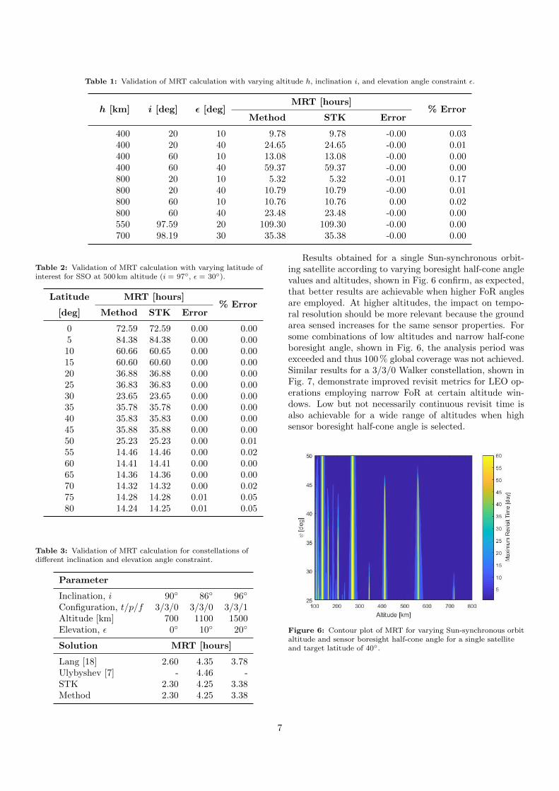
Table 1: Validation of MRT calculation with varying altitude h, inclination i, and elevation angle constraint ε.

h [km] i [deg] ε [deg]MRT [hours]

% ErrorMethod STK Error

400 20 10 9.78 9.78 -0.00 0.03400 20 40 24.65 24.65 -0.00 0.01400 60 10 13.08 13.08 -0.00 0.00400 60 40 59.37 59.37 -0.00 0.00800 20 10 5.32 5.32 -0.01 0.17800 20 40 10.79 10.79 -0.00 0.01800 60 10 10.76 10.76 0.00 0.02800 60 40 23.48 23.48 -0.00 0.00550 97.59 20 109.30 109.30 -0.00 0.00700 98.19 30 35.38 35.38 -0.00 0.00

Table 2: Validation of MRT calculation with varying latitude ofinterest for SSO at 500 km altitude (i = 97, ε = 30).

Latitude MRT [hours]% Error

[deg] Method STK Error

0 72.59 72.59 0.00 0.005 84.38 84.38 0.00 0.0010 60.66 60.65 0.00 0.0015 60.60 60.60 0.00 0.0020 36.88 36.88 0.00 0.0025 36.83 36.83 0.00 0.0030 23.65 23.65 0.00 0.0035 35.78 35.78 0.00 0.0040 35.83 35.83 0.00 0.0045 35.88 35.88 0.00 0.0050 25.23 25.23 0.00 0.0155 14.46 14.46 0.00 0.0260 14.41 14.41 0.00 0.0065 14.36 14.36 0.00 0.0070 14.32 14.32 0.00 0.0275 14.28 14.28 0.01 0.0580 14.24 14.25 0.01 0.05

Table 3: Validation of MRT calculation for constellations ofdifferent inclination and elevation angle constraint.

Parameter

Inclination, i 90 86 96

Configuration, t/p/f 3/3/0 3/3/0 3/3/1Altitude [km] 700 1100 1500Elevation, ε 0 10 20

Solution MRT [hours]

Lang [18] 2.60 4.35 3.78Ulybyshev [7] - 4.46 -STK 2.30 4.25 3.38Method 2.30 4.25 3.38

Results obtained for a single Sun-synchronous orbit-ing satellite according to varying boresight half-cone anglevalues and altitudes, shown in Fig. 6 confirm, as expected,that better results are achievable when higher FoR anglesare employed. At higher altitudes, the impact on tempo-ral resolution should be more relevant because the groundarea sensed increases for the same sensor properties. Forsome combinations of low altitudes and narrow half-coneboresight angle, shown in Fig. 6, the analysis period wasexceeded and thus 100 % global coverage was not achieved.Similar results for a 3/3/0 Walker constellation, shown inFig. 7, demonstrate improved revisit metrics for LEO op-erations employing narrow FoR at certain altitude win-dows. Low but not necessarily continuous revisit time isalso achievable for a wide range of altitudes when highsensor boresight half-cone angle is selected.

Figure 6: Contour plot of MRT for varying Sun-synchronous orbitaltitude and sensor boresight half-cone angle for a single satelliteand target latitude of 40.

7

Figure 7: Contour plot of MRT for varying Sun-synchronous orbitaltitude and sensor boresight half-cone angle for a 3/3/0constellation and target latitude of 40.

Major contributions to temporal resolution can also beguaranteed by off-nadir pointing capability when directcoverage between adjacent ground tracks is not achieved.The method does not directly address the effect of off-nadirpointing angle on MRT computation, but comparable re-sults can be obtained by increasing the FoR used.

Figure 8: MRT computation for varying Sun-synchronous orbitaltitude and target latitude for a single satellite with sensorboresight half-cone angle of 45.

For non-Earth-synchronous or repeat ground track or-bits, the projected ground track of a satellite appears tomove with respect to the Earth between subsequent orbits.As a consequence, consecutive passages over the equatorare separated in longitude, dependent on both the orbitalperiod and the rotation rate of the Earth [4]. For targetlatitudes approaching the poles (eg φ = 70), the distancebetween the lines of longitude diminishes and consequentlythe gaps which separate adjacent ground tracks from eachother at the target latitude are reduced for the same sen-sor properties, resulting in the expected improvement inMRT demonstrated in Fig. 8.

Figure 9: Contour plot of MRT for varying non-SSO orbitaltitude and inclination for a single satellite with sensor boresighthalf-cone angle of 45 and target latitude of 40.

Figure 10: Contour plot of MRT for varying non-SSO orbitaltitude and inclination for a single satellite with sensor boresighthalf-cone angle of 15 and target latitude of 40.

The impact of variation in angular FoR and orbit incli-nation for non-SSOs on temporal resolution is interesting.For a given altitude, the MRT is not constant for differ-ent inclinations due to the variation in ground-track shift,demonstrated in Fig. 9 and Fig. 10. These results alsodemonstrate that restriction of the angular FoR, by eithersensor selection or pointing capability, necessitates care-ful selection of the orbit inclination in coordination withthe altitude to obtain optimal revisit metrics even at alti-tudes greater than 600 km. However, for low FoR certainaltitude windows may need to be avoided, eg less than200 km and approximately 350 km and 500 km, where noinclination can be found that guarantees low revisit. Fur-thermore, for EO satellites which will experience orbitaldecay during their operational lifetime, consideration ofvariation in inclination may also be required in order tomaintain the optimal MRT.

8

4. Conclusions

This paper presents a semi-analytical method devel-oped for calculating revisit time for single satellite andconstellations in circular orbit with discontinuous cover-age. For the selected target latitude, the method providesa database where revisit metrics are calculated for vary-ing orbit altitudes, viewing or elevation angles, and in-clinations (in case of non-SSO) establishing a correlationbetween the longitude of the projected passages and theinstantaneous coverage of the sensor. Preliminary orbitand sensor geometry computation is carried out to deter-mine the sensor coverage in longitude at the target lati-tude. The maximum time difference between any two con-secutive passes over a selected target is then determinedthrough the computation of the longitudes crossing thelatitude of interest according to the satellite’s motion. Or-bital perturbations associated with the Earth’s oblatenessare considered through the J2 zonal spherical harmonics.Determination of visible longitudes is finally performed forvarying orbit configuration, sensor properties and orbitgeometry, defining a discretised grid of longitudes in theproximity of the selected latitude. The longitudes visibleat each pass are those which fall within the sensor foot-print projection on the Earth’s surface. For a matter ofsimplicity, the footprint is approximated with an ellipse,which is demonstrated to provide accurate results for thelatitude range of interest (< 75).

The method accuracy was validated by comparison toresults published in literature and STK numerical simula-tions. A maximum error of less than a minute was regis-tered in all cases, demonstrating the accuracy of the pre-sented method and the meaningful improvements achievedin revisit metrics computation compared to other analyt-ical routines. The computational efficiency of the methodwas also shown to be significantly better than widely avail-able commercial (numerical-based) software and similar tothat of other previously published information on analyt-ical methods, albeit using more modern hardware. Thecombination of these performance improvements will sup-port better early design phase analysis and more completedesign optimisation processes.

The capability of the method was demonstrated throughthe generation of plots that yield information on MRTcharacteristics for varying target latitudes, sensing capa-bilities, orbital parameters and configurations for both sin-gle satellite and Walker constellation architectures. Theseplots on their own and the supporting data can providevaluable reference for Earth observation system designersin the early phases of a mission development lifecycle.

Future developments of this method may include ex-tensions to single satellite and constellations in ellipticalorbits as well as non-symmetrical satellite constellations.Off-nadir pointing capabilities could also be directly ad-dressed, and the related impact on MRT computation dis-cussed. Calculation of revisit time metrics consideringtime of night/day or lighting conditions would also en-

able particular application for optical Earth observationsensors. Finally, more complex sensor shapes could beinvestigated and different projection geometries could bestudied to ensure accuracy of the method at higher targetlatitudes.

Acknowledgements

This work was supported by the Doctoral TrainingPartnership (DTP) between The University of Manchesterand the UK Engineering and Physical Sciences ResearchCouncil (EPSRC) under grant EP/M506436/1.

References

[1] M. A. Nunes, Satellite Constellation Optimization Method forFuture Earth Observation Missions using Small Satellites, Ad-vances in the Astronautical Sciences 146 (2013) 159–179, ISSN00653438.

[2] A. Marinan, A. Nicholas, K. Cahoy, Ad hoc Cube-Sat constellations: Secondary launch coverage and dis-tribution, in: IEEE Aerospace Conference, IEEE, BigSky, MT, ISBN 9781467318112, ISSN 1095323X, doi:10.1109/AERO.2013.6497174, 2013.

[3] S. Nag, J. LeMoigne, D. W. Miller, O. L. de Weck, A Frameworkfor Orbital Performance Evaluation in Distributed Space Mis-sions for Earth Observation, in: IEEE Aerospace Conference,IEEE, Big Sky, MT, ISBN 9781479953790, ISSN 1095323X, doi:10.1109/AERO.2015.7119227, 2015.

[4] J. R. Wertz, Orbit and Constellation Design, in: J. R. Wertz,W. J. Larson (Eds.), Space Mission Analysis and Design,chap. 7, Microcosm Press/Kluwer Academic Publishers, El Se-gundo, CA, 3 edn., 1999.

[5] J. R. Wertz, Orbit and Constellation Design Selecting the RightOrbit, in: J. R. Wertz, D. F. Everett, J. J. Puschell (Eds.),Space Mission Engineering: The New SMAD, chap. 10, Micro-cosm Press, Hawthorne, CA, 1 edn., 2011.

[6] M. S. Bottkol, P. B. DiDomenico, A Phase-Based Approach tothe Satellite Revisit Problem, in: AAS/AIAA Space Flight Me-chanics Meeting, American Astronautical Society (AAS), Hous-ton, TX, 865–884, 1991.

[7] Y. Ulybyshev, Geometric Analysis and Design Methodfor Discontinuous Coverage Satellite Constellations, Jour-nal of Guidance, Control, and Dynamics 37 (2) (2014)549–557, ISSN 0731-5090, doi:10.2514/1.60756, URLhttp://arc.aiaa.org/doi/10.2514/1.60756.

[8] Y. Ulybyshev, General Analysis Method for Discon-tinuous Coverage Satellite Constellations, Journal ofGuidance, Control, and Dynamics 38 (12) (2015) 2475–2483, ISSN 0731-5090, doi:10.2514/1.G001254, URLhttp://arc.aiaa.org/doi/10.2514/1.G001254.

[9] Y. N. Razoumny, Fundamentals of the route the-ory for satellite constellation design for Earth discon-tinuous coverage. Part 1: Analytic emulation of theEarth coverage, Acta Astronautica 128 (2016) 722–740,ISSN 00945765, doi:10.1016/j.actaastro.2016.07.013, URLhttp://dx.doi.org/10.1016/j.actaastro.2016.07.013.

[10] T. J. Lang, J. M. Hanson, Orbital Constellations which Min-imize Revisit Time, in: AAS/AIAA Astrodynamics Special-ists Conference, American Astronautical Society (AAS), LakePlacid, NY, 1983.

[11] T. J. Lang, A Parametric Examination of Satellite Constella-tions to Minimize Revisit Time for Low Earth Orbits using aGenetic Algorithm, Advances in the Astronautical Sciences 109I (2002) 625–640, ISSN 00653438.

9

[12] W. A. Crossley, E. A. Williams, Simulated Annealing and Ge-netic Algorithm Approaches for Discontinuous Coverage Satel-lite Constellation Design, Engineering Optimization 32 (3)(2000) 353–371, doi:10.1080/03052150008941304.

[13] M. P. Ferringer, D. B. Spencer, Satellite Constellation DesignTradeoffs Using Multiple-Objective Evolutionary Computation,Journal of Spacecraft and Rockets 43 (6) (2006) 1404–1411,ISSN 0022-4650, doi:10.2514/1.18788.

[14] M. P. Ferringer, R. S. Clifton, T. G. Thompson, Effi-cient and Accurate Evolutionary Multi-Objective OptimizationParadigms for Satellite Constellation Design, Journal of Space-craft and Rockets 44 (3) (2007) 682–691, ISSN 0022-4650, doi:10.2514/1.26747.

[15] O. Abdelkhalik, D. Mortari, Orbit Design for GroundSurveillance Using Genetic Algorithms, Journal of Guid-ance, Control, and Dynamics 29 (5) (2006) 1231–1235, ISSN 0731-5090, doi:10.2514/1.16722, URLhttp://arc.aiaa.org/doi/abs/10.2514/1.16722.

[16] O. Abdelkhalik, A. Gad, Optimization of spaceorbits design for Earth orbiting missions, ActaAstronautica 68 (7-8) (2011) 1307–1317, ISSN00945765, doi:10.1016/j.actaastro.2010.09.029, URLhttp://dx.doi.org/10.1016/j.actaastro.2010.09.029.

[17] D. A. Vallado, Fundamentals of Astrodynamics and Applica-tions, Microcosm Press/Springer, Hawthorne, CA, 4 edn., 2013.

[18] T. J. Lang, Walker Constellations to Minimize Revisit Time inLow Earth Orbit, in: 13th AAS/AIAA Space Flight MechanicsMeeting, American Astronautical Society (AAS), Ponce, PuertoRico, 2003.

10