A Self-tuning Failure Detection Scheme for CloudComputing Service

Naixue XiongDept. of Computer ScienceGeorgia State Univ., USA

E-mail: {nxiong, wsong, pan}@gsu.edu

Athanasios V. VasilakosDept. of Comp. and Tele. Engi.

Univ. of Western Macedonia, GreeceE-mail: vasilako@ath.forthnet.gr

Jie WuDept. of Comp. and Info. Scie.

Temple Univ., USA.E-mail: jiewu@temple.edu

Y. Richard YangDept. of Computer Science

Yale Univ.New Haven, USA

E-mail: yry@cs.yale.edu

Andy RindosIBM Corp., Dept. W4DA/Bldg 503

Research Triangle Park,Durham, NC, USA

E-mail: rindos@us.ibm.com

Yuezhi Zhou1,Wen-Zhan Song2,Yi Pan21Dept. of Comp. Scie. & Tech.

Tsinghua Univ., ChinaE-mail: zhouyz@mail.tsinghua.edu.cn

2Dept. of Computer ScienceGeorgia State Univ., USA

E-mail: {wsong, pan}@cs.gsu.edu

Abstract—Cloud computing is an increasingly important so-lution for providing services deployed in dynamically scalablecloud networks. Services in the cloud computing networks maybe virtualized with specific servers which host abstracted details.Some of the servers are active and available, while others arebusy or heavy loaded, and the remaining are offline for variousreasons. Users would expect the right and available servers tocomplete their application requirements. Therefore, in order toprovide an effective control scheme with parameter guidancefor cloud resource services, failure detection is essential to meetusers’ service expectations. It can resolve possible performancebottlenecks in providing the virtual service for the cloud com-puting networks. Most existing Failure Detector (FD) schemesdo not automatically adjust their detection service parametersfor the dynamic network conditions, thus they couldn’t beused for actual application. This paper explores FD propertieswith relation to the actual and automatic fault-tolerant cloudcomputing networks, and find a general non-manual analysismethod to self-tune the corresponding parameters to satisfyuser requirements. Based on this general automatic method,we propose a specific and dynamic Self-tuning Failure Detector,called SFD, as a major breakthrough in the existing schemes.We carry out actual and extensive experiments to compare thequality of service performance between the SFD and severalother existing FDs. Our experimental results demonstrate thatour scheme can automatically adjust SFD control parametersto obtain corresponding services and satisfy user requirements,while maintaining good performance. Such an SFD can beextensively applied to industrial and commercial usage, and itcan also significantly benefit the cloud computing networks.Index Terms—Application requirements, Cloud computing

service, Fault tolerance, Quality of service, Self-tuning failuredetection

I. INTRODUCTIONCloud computing provides resources to satisfy large num-

bers of user applications across networks [1-3]. Cloud com-puting networks [4-5] link users across the globe. For instance,they are being developed to support an education infrastructurefor student courses, learning labs, or connecting teachersand students to expert mentors [6]. Cloud models should

maintain high levels of Quality of Service (QoS) in accessinginformation remotely in network environments, and shouldensure users’ application security and dependability.In the cloud computing networks, some of the servers

may be active and available, while others are busy or heavyloaded, and the remaining may be offline or even crashedfor various reasons. Therefore, the cloud service environmentcan be dynamic and unexpected [7], and users would expectthe right and available servers to complete their applicationrequirements. We must be able to address the variabilityand provide an effective control scheme with parametersguidance to guide service conditions and cloud resources. Thusfault-tolerant schemes are designed to provide reliable andcontinuous services in cloud computing networks despite thefailures of some of their components [8-19]. As an essentialbuilding block for the cloud computing networks, a FailureDetector (FD) plays a critical role in the engineering of suchdependable network systems [19]. Effective failure detectionis essential to ensure acceptable QoS, and it is necessary tofind an optimized FD that can detect failures in a timely andaccurate way before a generic FD service can actually beimplemented for cloud computing network applications [20].For example, PlanetLab is a global cloud computing networkthat supports the development of new network services andit currently consists of 1076 nodes at 494 sites. While lotsof nodes are inactive at any time, yet we do not know theexact status (active, slow, offline, or dead). Therefore, it isimpractical to login one by one without any guidance.The design of reliable FDs is a very difficult task. One of the

main reasons is that the statistical behavior of communicationdelays is unpredictable. The other reason is that asynchronous(i.e., no bound on the process execution speed or message-passing delay) distributed systems make it impossible todetermine precisely whether a remote process is failed or hasjust been very slow [21]. An unreliable FD [21] can makemistakes like falsely suspecting correct processes or trusting

2012 IEEE 26th International Parallel and Distributed Processing Symposium

1530-2075/12 $26.00 © 2012 IEEE

DOI 10.1109/IPDPS.2012.126

668

2012 IEEE 26th International Parallel and Distributed Processing Symposium

1530-2075/12 $26.00 © 2012 IEEE

DOI 10.1109/IPDPS.2012.126

668

crashed processes. To ensure acceptable QoS for such anunreliable FD, parameters should be properly tuned to delivera desirable QoS at the upper layers, because the QoS of anFD greatly influences the QoS that upper layers may provide.Many fault-tolerant algorithms have been proposed (e.g., [19,22-27]), which are never-the-less based on unreliable FDs.A set of metrics are proposed to quantify the QoS of

an FD by Chen et al. in [28]: how fast it detects actualfailures and how well it avoids false detections. In order toimprove the QoS of an FD, a lot of adaptive FDs have beenproposed [29-32], such as Chen FD [28], Bertier FD [29, 33],and the φ FD [30-31]. Chen et al. in [28] proposed severalimplementations relying on the probabilistic behavior of thenetwork systems. The protocol uses arrival times sampled inthe recent past to compute an estimation of the arrival timeof the next heartbeat. However, a timeout that is set accordingto this estimation plus a constant safety margin, does notmatch the dynamic network behavior well [29]. Subsequently,Bertier FD [29, 33] provides an optimization of the safetymargin for Chen FD. It uses a different estimation function,combining Chen’s and Jacobson’s estimation of the Round-Trip Time (RTT). Bertier FD is primarily designed to beused over wired local area networks (LANs), where messagesare seldom lost [30]. The self-tuned FDs in [34-35] use thestatistics of the previously-observed communication delays tocontinuously adjust timeouts. In other words, they assumea weak past dependence on communication history. Thesethree FDs dynamically predict new timeout values based onobserved communication delays to improve the performanceof the protocols.Even though the above FDs had important technical break-

throughs, their success was limited. As far as we know, thereare three main reasons [30]: (1) an FD provides an informationlist of suspects about which processes have crashed. Thisinformation list is not always up-to-date or correct (e.g.,an FD may falsely suspect a process that is alive), due tothe high unpredictability of message delays, the dynamicand changing topology of a network system, and the highprobability of network message losses; (2) The conventionalbinary interaction (i.e., trust and suspect) makes it difficult tosatisfy the requirements of several distributed applications run-ning simultaneously. In practice, many classes of distributednetwork applications require the use of different QoS offailure detection to trigger different reactions (e.g., [36-37]).For instance, an application may take precautionary networkmeasures when the confidence in a suspicion reaches a givenlow level, while it takes successively more drastic actionsonce the doubt progresses to higher levels [10]. However, thetraditional output of the FDs (Chen FD [28] and Bertier FD[29, 33]) is of a binary nature1. (3) Most existing schemescan not automatically adjust their parameters for dynamicnetwork conditions, though users with an awareness of thescheme’s internal core functions and parameters can provide

1Bertier FD and Chen FD were aimed at other problems, which they bothsolved admirably well.

suitable values for the parameters based on the output QoS,which should satisfy the users’ expectation of QoS (QoS).This tuning may be very complex, and it is best done byprofessional engineers. Essentially, we are unable to usefixed parameters for FDs to satisfy user requirements in areliable way, where networks are dynamic and unexpected. Insum, the parameters used by existing failure detectors requireadjustment by hand, and so are not suitable for dynamicnetworks, especially in large scale distributed networks orunstable networks2. Therefore, we seek to further explore theFD properties and their inter-relations in providing an actualfault-tolerant distributed system.To attack the above problems, this paper firstly proposes

a general self-tuning failure detection method in the fault-tolerant cloud computing networks, and it can be extensivelyused for industrial and commercial purposes. In contrast, otherschemes could blindly provide different output QoS: some arejust temporarily suitable for the requirements; yet some arenever, then engineers have to manually change the relevantparameters. These schemes must try all the possible parametervalues, and get a performance output graph to know whichparameter values are acceptable for the network (manuallychoose relevant parameters). If the network has significantchanges, the engineers have to change the relevant parametersmanually again. Secondly, based on the above general method,we propose an automatic Self-tuning Failure Detector (SFD)to optimize the existing FDs, as an accural FD3. Thirdly, weexplore the implementation of SFD, which, briefly speaking,works as follows: A sliding window maintains the most recentsamples of the arrival time, similar to conventional adaptiveFDs [10, 28-29]. The next timeout delay τ approximation (fornext sample) is adjusted by the sliding window and feedbackinformation from the output. With this dynamic feedbackinformation, the relevant parameters are computed to matchrecent network conditions. By design, SFD can adjust well tohandle unexpected network conditions and the requirementsof any number of concurrently running applications. Finally,we comparatively evaluate our failure detection scheme andexisting schemes (Chen FD [28], Bertier FD [29, 33], and φFD [30-31]) by extensive experiments in seven representativeWide Area Network (WAN) cases. The experimental resultsshow the properties of the different FDs, and demonstrate thatour scheme can automatically adjust SFD control parametersto obtain corresponding services and satisfy user requirements,while maintaining good performance. Such an SFD can beextensively applied to industrial and commercial usage, and itcan also significantly benefit the cloud networks.The remaining content of the paper is organized as follows:

In Section II, the system model and failure detection QoSmetrics are introduced. Section III introduces several adaptiveFDs. In Section IV, we present a general self-tuning failure

2Here it means the networks have the high unpredictability of messagedelays, the great dynamic changing topology of system, or the high probabilityof message losses.3Accrual FD is when an FD service outputs a suspicion level on a

continuous scale rather than information of a boolean nature (trust vs suspect).

669669

SURA Cloud

HBCU Cloud

GA Education Cloud

GA Education Cloud

NC Education Cloud

NC Education Cloud

MD Education Cloud

MD Education Cloud

SC Education Cloud

SC Education Cloud

VA Education Cloud

VA Education Cloud

SURASURA

SURASURA

SURASURA

SURASURA

SURASURA

HBCUHBCU

GMU

GSU

NC State

UMBC

HBCUHBCU

HBCUHBCU

HBCUHBCU

HBCUHBCU

U of SC

Clemson

Cloud Users A

Cloud Users B

Fig. 1. Dynamic cloud computing network model: U.S. southern stateeducation cloud consortium (sponsored by IBM, SURA & TTP/ELC).

detection method for applicable engineering of such fault-tolerant cloud computing networks. Based on the generalmethod, we propose a SFD to optimize the existing FDs, andexplore the implementation of SFD. Section V carries out ex-periments in different network conditions (seven representativeWAN cases). In Section VI, we discuss more work related toFDs. Finally, we conclude our work and discuss further workin Section VII.

II. SYSTEM MODEL AND BASIC CONCEPTS

In this section, we first propose the practical cloud comput-ing network model (see Fig. 1) and academic cloud computingnetwork analysis model (see Fig. 2), and then define the failuredetection QoS metrics.

A. Practical Cloud Computing Network ModelAs shown in Fig. 1, we explore a dynamic cloud computing

network model4, which is based upon the United States south-ern states education cloud consortium and a network structurefor data centers [7]. Currently, five southern states (Georgia(GA), South Carolina (SC), North Carolina (NC), Virginia(VA), Maryland (MD)) have education cloud initiatives un-derway (Fig. 1). The multiple clouds could provide servicesto each other, such as depicted with users from the African-American Colleges and Universities (HBCU) community andusers from the Southeastern Universities Research Association(SURA), who may access the others’ resource (the curveddotted lines in Fig. 1). Guo et al. [7] has presented a similarfault-tolerant network structure for data centers, called DCell,where a DCell with a small server node degree can supportup to several million servers, just like the “Education cloud”

4In particular, we note that the general model can include multiple clouds.

in Fig. 1. Thus, Fig. 1 is an actual and representative cloudcomputing network model.As mentioned above, servers’ statuses may vary in cloud

computing networks: some are active, some busy or very slow,and some may be dead or crashed. Thus, a cloud failuredetection model is important to address failures of expectedservices by the corresponding servers, and initiate measures toensure appropriate service response. There are several existingFD schemes that could provide some detection services, whilenot by automatically adjusting their parameters for dynamicnetwork conditions. Therefore, this paper presents a generalself-tuning method to solve the above problem, and also givesan exact example based on the general method and the abovemodel.

B. A Theoretical Cloud Computing Network ModelHere we consider a partially synchronous cloud computing

network system consisting of a finite set of processes Π ={p1, p2, p3, ..., pn}5. A process may fail by crashing, here acrashed process does not recover. A process behaves correctly(i.e., according to the specification) until it (possibly) crashes.By definition, a correct process is a process that does not crash,and a faulty process is a process that is not correct.It is assumed that every pair of processes is assumed to

be connected by one unidirectional unreliable communicationchannel [17]. An unreliable channel is defined as a commu-nication channel: there is no message creation, no messagealteration and no message duplication, while it is possibleto lose some messages. Processes are completely connectedvia unidirectional communication channels. Without loss ofgenerality, this paper considers a simple system model (sameas [28-31, 33]) with only two processes, called p and q, whichare arbitrarily taken from the large system Π, where process qmonitors process p (see Fig. 2): p may periodically send amessage to q, perform local computation, or is subject tocrash6. Here the sending period is called the heartbeat intervalΔt. Process q may receive a message from p, or performlocal computation. q suspects process p if it can’t receive anyheartbeat message from p for a period of time determined bythe freshpoint (FP), which is given by the parameter (timeoutτ ).As illustrated in Fig. 2, di is the transmission delay of

heartbeat mi from p to q, and the sending period is calledthe heartbeat interval Δt. For the incoming heartbeat mi, qdynamically gives a response based on the new freshpointFPi. This model describes four cases that may occur. Thefirst one is that heartbeat message m1, from the sending timeσ1 of process p, arrives at q before q’s freshpoint FP1, thenq trusts p from the m1 arrival time (here we assume that p istrusted in the initial case). The second case is that the heartbeatmessage m2 from p is lost, then q waits for that heartbeat until

5This model is based on the above IBM cloud computing networks in Fig. 1.A user, a manager, or a total education cloud is regarded as a process.6Based on the theoretical cloud model in Fig. 1, here process q is like

a manager, and process p is like an education cloud. Then every educationcloud service environment is given by the monitoring results.

670670

its freshpoint FP2; after that, q starts to suspect p. The thirdcase is that heartbeatmi from p arrives at q after q’s freshpointFPi, then q suspects p from FPi until the mi arrival time.In the fourth case, after p sends out the heartbeat m(i+1), pis crashed. For the incoming heartbeat m(i+1), q computes anew freshpoint FPi+1 based on different FD schemes, andthen gives a response based on the heartbeat arrival time.Our SFD assumes the existence of some global time (un-

known to processes) denoted by global stabilized time, andthat processes always make progress. Furthermore, at leastδ > 0 time units elapse between consecutive steps (the purposeof the latter is to exclude the case where processes take aninfinite number of steps in finite time) [31]. The inter-processcommunication model is based on message exchanges overthe User Datagram Protocol (UDP) communication protocol.We don’t consider the relative speed of processes; however, weconsider that processes have access to a local clock device usedto measure the passage of time. Furthermore, every process hasaccess to a failure detection service.It is commonly believed that the period Δt is a factor

that contributes to the detection time. However, Muller [38]indicates that Δt is little determined by QoS requirements onseveral different networks, but much by the characteristics ofthe underlying system, and the work in [30] suggests that thereexists some nominal range for the parameter Δt with little orno impact on the accuracy of the FD in every network.The freshpoint is fixed in the conventional implementation

of this model. If the time between two next freshpoints is tooshort, the likelihood of a wrong suspicion rate is high, thoughcrashes are detected quickly. In contrast, if the time is toolong, there will be too much detection time, although thereare fewer inaccurate suspicions.Alternatively, this model can set the freshpoint based on the

transmission delay of the heartbeat. The advantage is that themaximal detection time is bounded, but the disadvantage isthat it relies on physical clocks with a negligible drift7 and ashared knowledge of the heartbeat interval Δt. The drawbackis a serious problem in practice: when the regularity of thesending of heartbeats cannot be guaranteed, and the actualsending interval is different from the target one (e.g., timinginaccuracies due to irregular OS scheduling) [30]. Both of themethods have their respective advantages and disadvantages,and it is difficult to conclude which one is better [30].

C. Failure detection QoS metrics

To quantitatively evaluate the QoS of FDs, we use threemain QoS metrics (i.e., detection time, mistake rate, andquery accuracy probability) that are independent [28]. The firstmetric measures the impact on the model from the speed ofthe FD, and the other two metrics relate to accuracy. In detail,considering two processes p and q where q monitors p, theQoS of the FD at q (called fdq) can be determined from

7A straightforward implementation of clocks requires synchronized clocks.Chen et al. [28] shows the method to do it with unsynchronized clocks, butthis still requires the drift between clocks to be negligible.

p

q

suspect

trust

tt

1d id

1 2 i 1i

1FP 2FP iFP 1iFPLost

1m 2m im

Boom

)1(im

Fig. 2. Basic heartbeat failure detection model.

up

down

suspect

trust

MT

MRT

DT

p

qfd

Fig. 3. Basic Metrics for the QoS evaluation of an FD [28].

its transitions between the “trust” and “suspect” states withrespect to p (see Fig. 38).Detection Time (TD): This is a random variable that

represents the length of a period from the time when p startscrashing to the time when q starts suspecting p permanentlyby fdq. Mistake Rate (MR): This is a random variable thatrepresents the number of mistakes that the failure detectormakes in a unit of time, i.e,. it represents how frequently thefailure detector makes mistakes. Query Accuracy Probability(QAP): This is a probability that, when queried at a randomtime, the FD at q indicates correctly that process p is up [28].Failure Detection QoS Definition Based on the work in

[39], a particular FD performance is defined in terms of itscompleteness and accuracy properties, and the QoS providedby each of its constituent failure detection modules is a tuple[39]:

QoS = (TD,MR, QAP ). (1)

The QoS quantifies both how fast a detector suspects a failureand how well it avoids false detection.

8In this Fig. 3, TM (Mistake duration) measures the time that elapses fromthe beginning of a wrong suspicion until its end (i.e., until the mistake iscorrected). TMR (Mistake recurrence time) measures the time between twoconsecutive wrong suspicions, it is a random variable representing the timethat elapses from the beginning of a wrong suspicion to the next one.

671671

III. EXISTING ADAPTIVE FAILURE DETECTORS

Recently, research studies have focused on the adaptiveFDs, whose goal is to adapt to changing network conditionsand application requirements [30]. In general, most adaptiveFDs are based on a heartbeat strategy, where recent historicalinformation is used to predict the arrival time of the nextheartbeat. Existing main adaptive FDs (Chen FD [28], BertierFD [29, 33], and φ FD [30-31]) work as follows:Chen FD Chen et al. [28] assumes that process p sends

heartbeat messages periodically to process q (see Fig. 2). Themost recent n heartbeat messages in a sliding window, denotedby m1, m2, ..., mn, are considered by process q. A1, A2, ...,An are their actual receiving times according to q’s local clock.When at least n messages have been received, the theoreticalarrival time EA(k+1) can be estimated by:

EA(k+1) =1n

k∑i=k−n−1

(Ai − Δi ∗ i) + (k + 1)Δi, (2)

where Δi is the sending interval. The next timeout delay(which expires at the next freshness point τ(k+1)) is composedof EA(k+1) and constant safety margin α. One has

τ(k+1) = α + EA(k+1). (3)

This technique provides an estimation for the next arrival timebased on a constant safety margin.Bertier FD Bertier et al. [29, 33] estimated the safety

margin is dynamically based on Jacobson’s estimation of theRTT [39]. Bertier FD adapts the safety margin α based on thevariable error in the last estimation. The recursive algorithm[29, 33] is as follows:

errork = Ak − EA(k) − delay(k), (4)

delay(k+1) = delay(k) + γ · error(k), (5)

var(k+1) = var(k) + γ · (|error(k)| − var(k)), (6)

α(k+1) = β · delay(k+1) + φ · var(k), (7)

and τ(k+1) = EA(k+1) + α(k+1), (8)

where the parameter γ represents the importance of the newmeasure with respect to the previous ones, the variable delayrepresents the estimate margin, and var estimates the magni-tude of errors. β and φ are used to adjust the variance var.Typical values of β, φ and γ are 1, 4 and 0.1, respectively.Bertier’s estimation provides a short detection time.

φ FD Different from the above schemes, the φ FD [30-31] outputs a suspicion level on a continuous scale, instead ofproviding information of a conventional binary nature (trust orsuspect). In this scheme, Tlast denotes the time when the mostrecent heartbeat was received; tnow is the current time; andPlater(t) denotes the probability that a heartbeat will arrivemore than t time units after the previous one. Then, the valueof φ is calculated as follows:

φ(tnow) = −lg(Plater(tnow − Tlast)). (9)

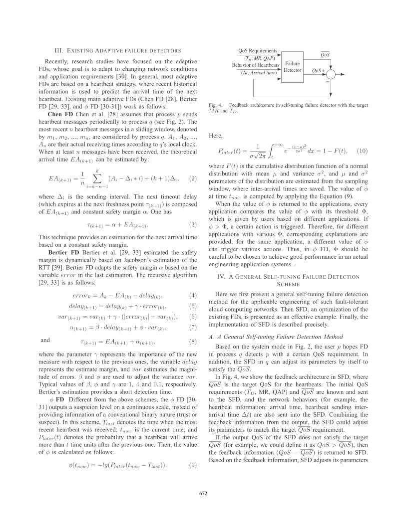
QoS Requirements

QoS

),,( QAPMRTD

Behavior of Heartbeats),( meArrival tit

QoS

Failure Detector

Fig. 4. Feedback architecture in self-tuning failure detector with the targetMR and TD .

Here,

Plater(t) =1

σ√

2π

∫ +∞

t

e−(x−μ)2

2σ2 dx = 1 − F (t), (10)

where F (t) is the cumulative distribution function of a normaldistribution with mean μ and variance σ2, and μ and σ2

parameters of the distribution are estimated from the samplingwindow, where inter-arrival times are saved. The value of φat time tnow is computed by applying the Equation (9).When the value of φ is returned to the applications, every

application compares the value of φ with its threshold Φ,which is given by users based on different applications. Ifφ > Φ, a certain action is triggered. Therefore, for differentapplications with various Φ, corresponding explanations areprovided; for the same application, a different value of φcan trigger various actions. Thus, in φ FD, Φ should becareful to be chosen to achieve good performance in an actualengineering application systems.

IV. A GENERAL SELF-TUNING FAILURE DETECTIONSCHEME

Here we first present a general self-tuning failure detectionmethod for the applicable engineering of such fault-tolerantcloud computing networks. Then SFD, an optimization of theexisting FDs, is presented as an effective example. Finally, theimplementation of SFD is described precisely.

A. A General Self-tuning Failure Detection MethodBased on the system mode in Fig. 2, the user p hopes FD

in process q detects p with a certain QoS requirement. Inaddition, the SFD in q can adjust its parameters by itself tosatisfy the QoS.In Fig. 4, we show the feedback architecture in SFD, where

QoS is the target QoS for the heartbeats. The initial QoSrequirements (TD, MR, QAP) and QoS are known and sentto the SFD, and the network behaviors (for example, theheartbeat information: arrival time, heartbeat sending inter-arrival time Δt) are also sent into the SFD. Combining thefeedback information from the output, the SFD could adjustits parameters to match the target QoS requirement.If the output QoS of the SFD does not satisfy the target

QoS (for example, we could define it as QoS > QoS), thenthe feedback information (QoS − QoS) is returned to SFD.Based on the feedback information, SFD adjusts its parameters

672672

QoSRequirements

MR

00

DT

QoS

Fig. 5. Parameter relation of self-tuning failure detection, QoS is the targetQoS for the heartbeats.

(for example, timeout τ for the timeout-based schemes). Then,eventually SFD can satisfy the QoS (if there is a certain rangefor this SFD, where SFD can satisfy the QoS). Otherwise, ifthe QoS is too high, and this SFD could not find suitableparameters for it, then the SFD will give a response: “ThisSFD can not satisfy the QoS for the application”.For more details, if we focus on the three main parameters

in QoS: TD, MR, and QAP (the performance parameters fora period experiment, not for a time slot), then the output QoSof SFD is based on all the former time periods.In Fig. 5, we show the parameter relation of self-tuning

failure detection, where the target MR and TD should besmaller than the required values of MR and TD, and the QAPshould be larger than the required values of QAP.In effect, in a specific time slot, we adjust the parameters of

SFD only one time, based on feedback information, to improvethe output QoS of SFD to close the QoS. Usually we haveto repeatedly adjust the parameters of SFD in multiple timeslots to improve the output QoS gradually, and finally find theproper parameters to satisfy the QoS. At that time, the SFDstabilizes the parameters of SFD and cloud communicationnetwork systems. If systems have great changes and theresponding output QoS does not satisfy the QoS, then theSFD will give feedback information to improve output QoSof SFD gradually again until the output QoS of SFD satisfiesthe QoS. Here we assume the experimental time is longenough to let output QoS of SFD satisfy the QoS for theapplications and the proper control parameters are existingand available. This method is general, and can be applied tothe other adaptive timeout-based FD schemes. In summary, weshould first get the output QoS (TD, MR, and QAP ) basedon the traditional detection scheme [28], and then try to getthe feedback information to adjust the relevant parameters inSFD.

B. Self-tuning Failure DetectorBased on the above general self-tuning failure detection

method, here we present a material SFD for the engineeringapplication, which also optimizes the existing failure detectorsas an example.Here, we combine the Chen FD [28] and φ FD [30-31]

schemes. Because Chen FD [28] has an extensive performancerange, it could achieve better performance in a conservative

range than φ FD and Bertier FD [29, 33], and also achievesimilar performance to φ FD in an aggressive range. φ FDis available in only the aggressive range because its roundingerrors prevent to compute points in the conservative range.Bertier FD has no dynamic parameter, and has only oneaggressive performance value. Furthermore, φ FD outputs asuspicion level on a continuous scale (not traditional binaryinformation), and could provide different QoS of failure de-tection to trigger different reactions.SFD adjusts the next predictable freshness point τ(k+1)

based on the feedback information. Therefore, we have

τ(k+1) = SM(k+1) + EA(k+1), (11)

where EA(k+1) is the same as the parameter in Chen-FD,while SM is the dynamic safety margin, and can be adjustedto satisfy the predefined QoS. Here, we have

SM(k+1) = SMk + Satk{QoS,QoS} · α, (12)

where the α (α ∈ (0, 1)) is the same as the constant safetymargin in Chen-FD, and we set

Satk{QoS,QoS} ={ ±β, QoS > QoS;

0, QoS ≤ QoS.(13)

where β is a constant value, and β ∈ (0, 1), and based on thespecific output QoS status, Satk{QoS,QoS} could be set asβ, −β, or 0. The value β is for the adjusting rate, and it couldbe dynamically chosen by users.From Functions (11-13), a larger α value will lead to larger

TD, shorter MR, and larger QAP in our SFD (because alarger α value provides a larger safety margin). To this point,our scheme is similar to Chen-FD. To choose the Satk{QoS,QoS}, we focus on the two aspects: response time (TD)and detection precision (MR and QAP ). We should makea compromise between response time and detection precisionto match the target QoS QoS. For example, if we try to shortenresponse time, and then this adjusting will worsen the detectionprecision, and vice versa.From a theoretical view, SFD satisfies the property of

the accrual failure detector [31], and also belongs to theclass ♦Pac (accruement property and upper bound property),which is sufficient to solve the consensus problem.

C. The Implementation of SFDThis section first describes the architecture of SFD, then

presents its specific implementation algorithm.1) The Architecture of SFD: Conceptually, the implemen-

tation of SFD can be decomposed into three basic parts:Monitoring, Interpretation, and Action [30].In traditional timeout-based FDs (Chen FD [28] and Bertier

FD [29, 33]), the monitoring and the interpretation are com-bined within the FD, and the output is binary. However, SFD,as an accrual FD [30-31], provides a lower-level abstractionthat avoids the interpretation of monitoring information. Somevalues, the suspicion level associated with each process, areleft for the applications to interpret [30].

673673

Application processes set a suspicion threshold according totheir own QoS requirements: a low threshold generates manywrong suspicions, but quickly detects an actual crash. Con-versely, a high threshold is prone to generate fewer mistakes,but needs more time to detect actual crashes.2) The Implementation of SFD: As an accrual FD, the

method used in SFD is quite simple. After a warm-up period,when a new heartbeat arrives, the inter-arrival time is put intoa sampling sliding window, and at the same time, the previousoldest one is pushed out of the sampling window. Then thearrival time in the sampling window is used to compute thedistribution of inter-arrival times, and get the average inter-arrival time Δt in this sliding window. After that, based onEquations (11-13), we compute the current value of timeout τ ,which gives the next freshness point (see Fig. 2). Applicationswill perform some actions, or start to suspect the process bycomparing the τ value and its current heartbeat arrival time(see Fig. 2).We are unable to get the communication delay from the

sender to the receiver when it is lost (see the second case inFig. 2). In order to ensure the effectiveness of the proposedapproach, and considering the influence of message loss, weuse the time series theory to fill in the gap. In detail, we fillin the gaps with a value computed by di = (Δt ·nag)+di−1,where nag is the average number of observed adjacent gaps[18].The detailed information for the implementation of SFD

is shown in Algorithm 1. Here we first set some initialparameters, including an initial safety margin value for SM1.After that, SFD could get the feedback information (Step 2in Algorithm 1): If SM1 is the proper parameter for SFD toobtain the expected output QoS, then the feedback informationis 0, and the SFD is stable. This means the current parametersare proper for the network system; If SM1 is not the exactproper parameter for SFD to acquire the expected outputQoS and the output QoS matches the control rules, then thefeedback information is ±β based on specific output QoSstatus; If SM1 is not the exact proper parameter for SFD toacquire the expected output QoS and the output QoS does notmatch the control rules, then the SFD give a response aboutthis mistake (all the possible values are not proper for SM1).Finally, if the SFD does not show “give a response”, SFDadjusts the parameter SM until gets the expected output QoS.For Chen FD [28], they have to find the exact proper

parameter value for its initial safety margin to achieve theexpected output QoS (because they could not automaticallyadjust the parameter); Otherwise, the output QoS can notsatisfy the QoS (users’ requirements). The φ FD [30-31] andBertier FD [29, 33] also have same drawback, which is solvedby our SFD.

V. PERFORMANCE EVALUATIONIn order to demonstrate that the presented general non-

manual analysis method in this paper is effective, we evaluateand comparatively analyze the performance of SFD, φ FD[30-31], Chen FD [28], and Bertier FD [29, 33] in general

Algorithm 1 A Method to Adjust the Parameters1: Begin2: Initialization:3: TD: Set the detection time;4: MR: Set the mistake rate;5: QAP : Set the query accuracy probability;6: Set the initial safety margin value for SM1;7: Set the constant parameters α, and β;8: Step 1: Get the relevant data9: Get the output QoS (TD , MR, QAP).10: Step 2: Get the feedback information11: If TD > TD , MR < MR, and QAP > QAP :

Satk{QoS, QoS} = β;12: If TD < TD , MR < MR, and QAP > QAP :

Satk{QoS, QoS} = 0;13: If TD < TD , MR > MR, and QAP < QAP :

Satk{QoS, QoS} = −β;14: Others (for example, if TD > TD , and MR > MR): “Give

a response” (this SFD can not get this high QoS requirement),and stop SFD (go to line 18).

15: Step 3: Adjust parameters16: Send Satk{QoS, QoS} to the SFD;17: Adjust SFD relevant parameters based on the value of

Satk{QoS, QoS};18: End

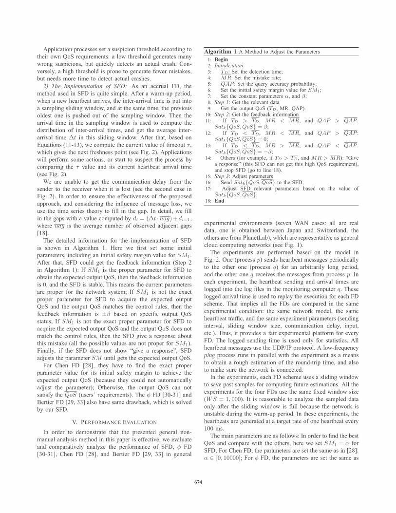
experimental environments (seven WAN cases: all are realdata, one is obtained between Japan and Switzerland, theothers are from PlanetLab), which are representative as generalcloud computing networks (see Fig. 1).The experiments are performed based on the model in

Fig. 2. One (process p) sends heartbeat messages periodicallyto the other one (process q) for an arbitrarily long period,and the other one q receives the messages from process p. Ineach experiment, the heartbeat sending and arrival times arelogged into the log files in the monitoring computer q. Theselogged arrival time is used to replay the execution for each FDscheme. That implies all the FDs are compared in the sameexperimental condition: the same network model, the sameheartbeat traffic, and the same experiment parameters (sendinginterval, sliding window size, communication delay, input,etc.). Thus, it provides a fair experimental platform for everyFD. The logged sending time is used only for statistics. Allheartbeat messages use the UDP/IP protocol. A low-frequencyping process runs in parallel with the experiment as a meansto obtain a rough estimation of the round-trip time, and alsoto make sure the network is connected.In the experiments, each FD scheme uses a sliding window

to save past samples for computing future estimations. All theexperiments for the four FDs use the same fixed window size(WS = 1, 000). It is reasonable to analyze the sampled dataonly after the sliding window is full because the network isunstable during the warm-up period. In these experiments, theheartbeats are generated at a target rate of one heartbeat every100 ms.The main parameters are as follows: In order to find the best

QoS and compare with the others, here we set SM1 = α forSFD; For Chen FD, the parameters are set the same as in [28]:α ∈ [0, 10000]; For φ FD, the parameters are set the same as

674674

in [30-31]: Φ ∈ [0.5, 16]; For Bertier FD, the parameters areset the same as in [29, 33]: β = 1, φ = 4, γ = 0.1. In eachexperiment, the other basic experimental parameters of FDsare the same.In these experiments, after discarding some initial period,

we have measured the following three key QoS metrics forthe entire execution: TD, MR, QAP. It is not easy to compareparametric failure detectors because, depending on the valueset for their parameter, their behaviors can be completelydifferent. A common mistake is to set some arbitrary valuesfor the parameters and then compare two parametric failuredetectors based on the measured detection time and accuracy.This almost always leads to the erroneous conclusion that oneis better for detection time while the other provides higheraccuracy.In contrast, we use the developed approach when conducting

experiments for the φ FD [30-31]. The idea is based on thefollowing question: given a set of QoS requirements, can thefailure detector be parameterized to match these requirements?To answer this question, we consider a space of QoS definedby the detection time on one axis and an accuracy metric (e.g.,MR, or QAP ) on the other axis. Then, we measure the areacovered by the failure detector when we vary its parameterfrom a highly aggressive behavior to a very conservative one(i.e., TD becomes larger and larger9.). The area covered by afailure detector is the area that corresponds to a set of QoSrequirements that can possibly be matched by that failuredetector. In each experiment, different output values (MR,QAP and TD) were obtained from the following respectiveparameters: For SFD, a list about the initial safety margin SM1

is given, and other parameters including α and β are not listedfor that they only impact the rate of self-tuning adjustability;For Chen FD, a list about the initial safety margin is given;For φ FD, a list about the threshold parameter Φ is given.We find that when the parameter continuously changes in

sequential order (for example, from the small value to the largevalue), the graph is serially developing, and we can obtainplenty of points, which can be fitted on this curve graph.

A. Experiment in a WAN

This experiment involves two computers: one was located atthe Swiss Federal Institute of Technology in Lausanne (EPFL),in Switzerland, and the other was located in JAIST, Japan. Thetwo computers communicate with each other through a normalintercontinental Internet connection.In this experiment, we use exactly the same trace files from

the paper about φ FD [30-31], and these trace files are publiclyavailable on the lab website [40]. Therefore, this provides acommon ground for evaluating the performances of SFD, ChenFD [28], Bertier FD [29, 33], and φ FD [30-31].

9Here each point in the graph is corresponding to a parameter in this FDscheme. When we choose the parameter in order (for example, from the smallvalue to the large value), we could get a lot of points which can be fitted witha serial curve.

0 0.2 0.4 0.6 0.8 110

−4

10−3

10−2

10−1

Detection time [s]

Mis

take

ra

te [

1/s

]

SFDChen FDBertier FDφ FDφ FD

Chen FD

SFD

Bertier FD

Fig. 6. Mistake rate vs. detection time in a WAN.

1) Experiment Setting: Hardware/software/network: In de-tail, the trace files and relevant data were obtained from thefollowing experiment setting.Heartbeat sampling The experiment was over in one week

(started on April 3 at 2:56 UTC, and finished on April 10at 3:01 UTC). During the experimental period, the aver-age sending rate actually measured was one heartbeat every103.501 ms (standard deviation: 0.189 ms; min.: 101.674 ms;max.: 234.341 ms). Furthermore, only 5, 822, 521 out of the5, 845, 713 heartbeat messages sent out were received, thusthe message loss rate was about 0.399%. After checking thetrace files more carefully, the messages losses were due to 814different bursts. The majority of total bursts were short lengthbursts, while the maximum burst-length was 1, 093 heartbeats(only one), and it lasted about 2 minutes. Furthermore, mostof the heartbeats were not directly from Asia to Europe, butactually, routed through the United States.Round-trip time The average RTT is 283.338ms, with a

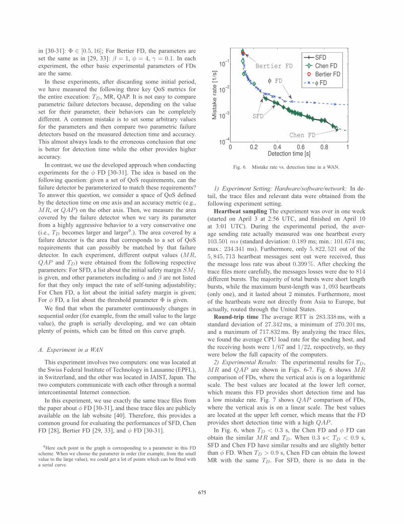
standard deviation of 27.342ms, a minimum of 270.201ms,and a maximum of 717.832ms. By analyzing the trace files,we found the average CPU load rate for the sending host, andthe receiving hosts were 1/67 and 1/22, respectively, so theywere below the full capacity of the computers.2) Experimental Results: The experimental results for TD,

MR and QAP are shown in Figs. 6-7. Fig. 6 shows MRcomparison of FDs, where the vertical axis is on a logarithmicscale. The best values are located at the lower left corner,which means this FD provides short detection time and hasa low mistake rate. Fig. 7 shows QAP comparison of FDs,where the vertical axis is on a linear scale. The best valuesare located at the upper left corner, which means that the FDprovides short detection time with a high QAP .In Fig. 6, when TD < 0.3 s, the Chen FD and φ FD can

obtain the similar MR and TD. When 0.3 s< TD < 0.9 s,SFD and Chen FD have similar results and are slightly betterthan φ FD. When TD > 0.9 s, Chen FD can obtain the lowestMR with the same TD. For SFD, there is no data in the

675675

0 0.2 0.4 0.6 0.8 1 1.299.6

99.65

99.7

99.75

Detection time [s]

Qu

ery

accu

racy p

rob

ab

ility

[%

]

SFDChen FDφ FD

SFD

Chen FD

φ FD

Fig. 7. Query accuracy probability vs. detection time in a WAN.

too aggressive range (TD < 0.3 s) and the too conservativerange (TD > 0.9 s). Since SFD can dynamically adjust itsparameters.At the beginning, the initial safety margin SM1 was set as

a very small value, then output QoS in our SFD had a shortdetection time TD (TD < TD) and a large mistake rate MR(MR > MR). It implies the output QoS does not satisfy theQoS, and we should take multiple steps to increase SM inorder to reduce theMR. Then, our scheme gradually increasedSM in next multiple freshness points τ to reduce the MR ofoutput QoS. Eventually, we satisfy theQoS for the application.For the next SM1 value, which is slightly larger than the

former one10, SFD first had a lower MR than the formerone (with a lower SM1 value), which was still larger thanMR. Then our scheme multiple increases SM to graduallyget lowerMR of output QoS, as far as the output QoS satisfiesthe QoS. So for the total output QoS, usually a larger SM1

leads to a larger TD, a lower MR and a higher QAP . Butit is not absolute, because the SFD could automatically adjustthe SM to satisfy the QoS.Interestingly, there are some bursts in this WAN experiment,

so for every SM1 value, after the output QoS of SFD has beenadjusted to satisfy the QoS, due to the bursts, there were somefluctuations for the output QoS of SFD.For those SM1 values with TD > 0.9 s in SFD, our scheme

can reduce the SM in next freshness point τ to get shorterTD gradually, though it leads to slightly larger MR. If thefirst output TD is greater than 0.9 s in SFD (because theSM1 is very large), we should spend more steps to reducethe SM to reduce TD, and let TD < TD eventually. Then intotal performance, output MR is larger and TD is shorter. Itis reasonable for those SM1 values with TD > 0.9 s that,when SFD’s SM1 increases, TD becomes larger and MRbecomes lower. The graphs of φ FD are stopped early (at

10In our SFD experiments, SM1 gradually increases from a list of possiblevalues.

2.43 s), due to the rounding error preventing the graphs to thevery conservative case. For Bertier FD, it has only one pointbecause it has no dynamic parameters. This is the same statusin other experimental environments. In Fig. 7, we have similarresults to the Fig. 6.

B. Extensive PlanetLab WAN Experiments

We have analyzed the behavior of the implementation ofthe SFD in a large collection of environments. Here wefocus on the most relevant WAN environments in order toobtain the general experimental analysis. The main goal ofour experiments was to observe the performance of the SFDto be automatically configured well to match the QoS. In thiscase, we compare SFD against Chen-FD, Bertier-FD, and φ-FD. Here we first describe the various WAN environments, andthen make comparison between SFD and existing FDs usingfeasible methods, and finally the relevant results are discussed.1) Experiment Settings: The experimental environments

are described below, and the corresponding statistics aresummarized in Table I and Table II. Here six representa-tive WAN experiments were conducted on the PlanetLab(http://www.planet-lab.org/), using nodes located in USA, Eu-rope (Germany), Japan, and China (Hong Kong). Each locationcommunicates with the other three locations (see Fig. 8 andTables I-II). The locations and hostnames are summarized inTable I. Each WAN experiment was set to last for about 24hours, with a target heartbeat interval set to 10 ms.Environment 1 (WAN-1). This set was from Stanford

University, USA to Nara Institute of Science and Technology,Japan, starting from March 12, 2007. The effective heartbeatinterval was 12.825 ms, and total 6, 737, 054 heartbeats weresent. The mean heartbeat arrival time was 12.83 ms (thusshowing a slight clock drift) with a standard deviation of14.892 ms. The average round-trip time was 193.909 ms.Environment 2 (WAN-2). This set was from Germany to

USA, starting from March 8, 2007. Total 7, 477, 304 heartbeatswere sent, and the loss rate was 5%.Environment 3 (WAN-3). This set was from Japan to

Germany, starting from March 6, 2007. Total 7, 104, 446heartbeats were sent, and the loss rate was 2%.Environment 4 (WAN-4). This set was from Hong Kong

(China) to USA, starting from March 10, 2007. Total 7, 028,178 heartbeats were sent, and the loss rate was 0%.Environment 5 (WAN-5). This set was from Hong Kong

(China) to Germany, starting from March 11, 2007. Total 7,008, 170 heartbeats were sent, and the loss rate was 4%.Environment 6 (WAN-6). This set was from Hong Kong

University of Science and Technology, Hong Kong to MuralLabolatory, Keio University Shonan Fujisawa Campus, Japan.Total 7, 040, 560 heartbeats were sent, and the loss rate was0%.As a final note, we use the ping process conducted in

parallel with the experiments to obtain the ping log files, whichdemonstrate that the Network was always connected duringexperiments.

676676

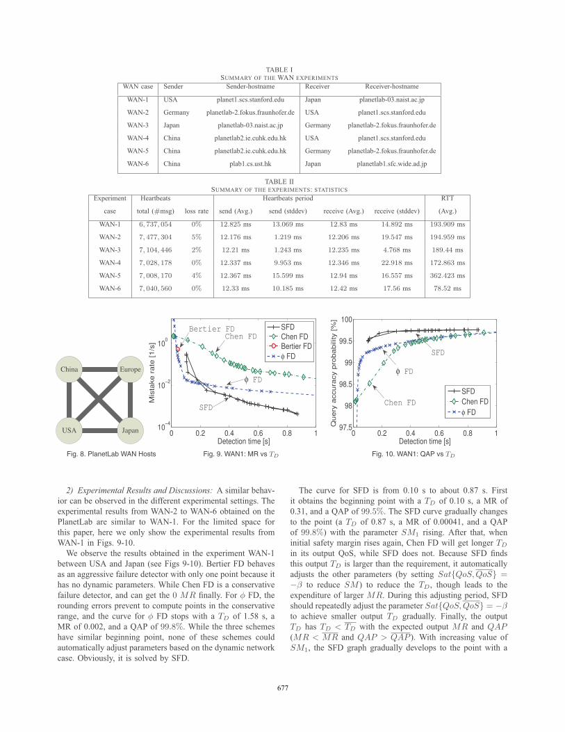
TABLE ISUMMARY OF THE WAN EXPERIMENTS

WAN case Sender Sender-hostname Receiver Receiver-hostname

WAN-1 USA planet1.scs.stanford.edu Japan planetlab-03.naist.ac.jp

WAN-2 Germany planetlab-2.fokus.fraunhofer.de USA planet1.scs.stanford.edu

WAN-3 Japan planetlab-03.naist.ac.jp Germany planetlab-2.fokus.fraunhofer.de

WAN-4 China planetlab2.ie.cuhk.edu.hk USA planet1.scs.stanford.edu

WAN-5 China planetlab2.ie.cuhk.edu.hk Germany planetlab-2.fokus.fraunhofer.de

WAN-6 China plab1.cs.ust.hk Japan planetlab1.sfc.wide.ad.jp

TABLE IISUMMARY OF THE EXPERIMENTS: STATISTICS

Experiment Heartbeats Heartbeats period RTT

case total (#msg) loss rate send (Avg.) send (stddev) receive (Avg.) receive (stddev) (Avg.)

WAN-1 6, 737, 054 0% 12.825 ms 13.069 ms 12.83 ms 14.892 ms 193.909 ms

WAN-2 7, 477, 304 5% 12.176 ms 1.219 ms 12.206 ms 19.547 ms 194.959 ms

WAN-3 7, 104, 446 2% 12.21 ms 1.243 ms 12.235 ms 4.768 ms 189.44 ms

WAN-4 7, 028, 178 0% 12.337 ms 9.953 ms 12.346 ms 22.918 ms 172.863 ms

WAN-5 7, 008, 170 4% 12.367 ms 15.599 ms 12.94 ms 16.557 ms 362.423 ms

WAN-6 7, 040, 560 0% 12.33 ms 10.185 ms 12.42 ms 17.56 ms 78.52 ms

China Europe

JapanUSA 0 0.2 0.4 0.6 0.8 110

−4

10−2

100

Detection time [s]

Mis

take r

ate

[1/s

]

SFDChen FDBertier FDφ FD

φ FD

Bertier FD

SFD

Chen FD

0 0.2 0.4 0.6 0.8 197.5

98

98.5

99

99.5

100

Detection time [s]

Qu

ery

accu

racy p

rob

ab

ility

[%

]

SFDChen FDφ FD

SFD

φ FD

Chen FD

Fig. 8. PlanetLab WAN Hosts Fig. 9. WAN1: MR vs TD Fig. 10. WAN1: QAP vs TD

2) Experimental Results and Discussions: A similar behav-ior can be observed in the different experimental settings. Theexperimental results from WAN-2 to WAN-6 obtained on thePlanetLab are similar to WAN-1. For the limited space forthis paper, here we only show the experimental results fromWAN-1 in Figs. 9-10.We observe the results obtained in the experiment WAN-1

between USA and Japan (see Figs 9-10). Bertier FD behavesas an aggressive failure detector with only one point because ithas no dynamic parameters. While Chen FD is a conservativefailure detector, and can get the 0 MR finally. For φ FD, therounding errors prevent to compute points in the conservativerange, and the curve for φ FD stops with a TD of 1.58 s, aMR of 0.002, and a QAP of 99.8%. While the three schemeshave similar beginning point, none of these schemes couldautomatically adjust parameters based on the dynamic networkcase. Obviously, it is solved by SFD.

The curve for SFD is from 0.10 s to about 0.87 s. Firstit obtains the beginning point with a TD of 0.10 s, a MR of0.31, and a QAP of 99.5%. The SFD curve gradually changesto the point (a TD of 0.87 s, a MR of 0.00041, and a QAPof 99.8%) with the parameter SM1 rising. After that, wheninitial safety margin rises again, Chen FD will get longer TD

in its output QoS, while SFD does not. Because SFD findsthis output TD is larger than the requirement, it automaticallyadjusts the other parameters (by setting Sat{QoS,QoS} =−β to reduce SM ) to reduce the TD, though leads to theexpenditure of larger MR. During this adjusting period, SFDshould repeatedly adjust the parameter Sat{QoS,QoS} = −βto achieve smaller output TD gradually. Finally, the outputTD has TD < TD with the expected output MR and QAP(MR < MR and QAP > QAP ). With increasing value ofSM1, the SFD graph gradually develops to the point with a

677677

TD of 0.10 s, a MR of 0.0.31, and a QAP of 99.5%, whichis very close to the beginning point.The optimization of SFD over φ FD, Bertier FD, and Chen

FD is significant: Although sometimes SFD does not providethe better performance than other FDs (for example, whenDT is smaller than about 0.2 s, φ FD get lower MR thanSFD does at the same DT ), yet only SFD could automaticallyadjust its parameters to match the QoS. Specifically, withinitial safety margin SM1 rising, SFD can always automati-cally adjust Sat{QoS,QoS} and find suitable SM to get asatisfactory output QoS for users’ requirements. In contrast,other schemes could blindly provide different output QoS:some are just temporarily suitable for the requirements; yetsome are never, then engineers have to manually change therelevant parameters. These schemes must try all the possibleparameter values, and get a performance output graph toknow which parameter values are acceptable for the network(manually choose relevant parameters). If the network hassignificant changes, the engineers have to change the relevantparameters manually again. In conclusion, SFD has goodself-tuning property, and it can be more effectively used incloud computing environments for extensive industrial andcommercial usage.The parameter settings in each FD are key factors, since a

different parameter setting could lead to a completely differentresults. For a qualitative analysis, when the parameter contin-uously changes in a fixed order (for example, from the smallvalue to the large value), the graph serially monotonouslydevelops in most cases11. There is no quantitative relationshipbetween the parameter change and the results change, becausethey are independent.In summary, we evaluate the performance of SFD in a

variety of WAN environments (see Fig. 8). Experimentalresults have shown that the SFD can automatically adjustparameters to provide good performance at general networkcases over other state-of-the-art failure detectors.

C. Comparative Analysis of the Four FDsAll our above experiments cover the most representative

application environment found at present. Based on them, weconclude the following:Self-tuning property: The experiments demonstrate that SFD

outperforms the existing FDs (φ FD [30-31], Bertier FD [29,33], and Chen FD [28]) in terms of self-tuning capacity.Specifically, in cloud computing networks, with initial safetymargin SM1 rising, SFD can always automatically adjustSat{QoS,QoS} and find suitable SM to get a satisfactoryoutput QoS for users’ requirements. In contrast, other schemescould blindly provide different output QoS. If the network hassignificant changes, the engineers have to change the relevantparameters manually again.Effect of window size: We analyze the effect of window

size on QoS of FDs. For φ FD, a larger window size tends toachieve better performance [41]. The possible reason is that

11The possible reason for the abnormal cases is that some burst data andtoo old data affect the output QoS.

historical information is important for φ FD to get good QoS.φ FD is based on the normal distribution function, so the largersize window could obtain more historical data, and so computemore adaptive normal distribution function for the relevantnetwork case. For Bertier FD, the effect of window size ontheir QoS can be negligible. The possible reason is that BertierFD has no tuning parameters. For Chen FD and SFD, a lowerwindow size leads to better performance [41]. Chen FD isbased on Functions (2) and (3), and SFD is based on Functions(2) and (11-13). When window size increases, there are morehistorical data for Chen FD and SFD based on Function (2),and the many burst data and too old data may affect the outputQoS, making less ideal contributions (even bad contributions)for achieving good performance. Chen FD and SFD take lesstime to adapt the dynamic network with a reduced windowsize.In summary, SFD is a practical self-tuning FD which can

be effectively used for industrial and commercial applicationto automatically satisfy QoS for users’ requirements. Further-more, SFD has good scalability. Because it is able to getacceptable performance with very small window size, and itcan save valuable memory resources. All the evidence supportsour conclusion that the general self-tuning failure detectionanalysis of SFD is effective.

VI. CONCLUSION AND FUTURE WORK

Services in the distributed networks may be virtualized withspecific servers. Some of the servers are active and available,while others are busy or heavy loaded, and the remaining areoffline for various reasons. Users would expect the right andavailable servers to complete their application requirements.Therefore, in order to provide an effective control scheme andparameters guidance for service conditions, failure detectionis essential to meet users’ service expectations. Most existingFailure Detector (FD) schemes do not automatically adjusttheir detection service parameters for the dynamic networkconditions, thus they couldn’t be used for actual application.This paper explores FD properties with relation to the actualand automatic fault-tolerant cloud computing networks, andfind a general non-manual analysis method to self-tune thecorresponding parameters to satisfy users’ requirements. Basedon this general automatic method, we propose a specific anddynamic Self-tuning Failure Detector scheme, called SFD,as a major breakthrough in the existing schemes. We carryout actual and extensive experiments to compare the qual-ity of service performance between the SFD and severalother existing FDs. Experimental results demonstrate that ourscheme can automatically adjust SFD control parameters toobtain corresponding services and satisfy user requirements,while maintaining good performance. Such an SFD can beextensively applied to industrial and commercial usage, and itcan also significantly benefit the cloud computing networks.Our SFD is also appropriate for the “one monitors multiple”and “multiple monitor multiple” cases based on the paralleltheory. In our future work, we would like to explore software

678678

engineering solutions in the United States southern stateseducation cloud consortium (see Fig. 1).

VII. ACKNOWLEDGMENTSThis research has been supported in part by the IBM Faculty

Award from IBM Cloud Academy, NC; partially supportedby China National Science Foundation (NSF): Adaptive andDynamic Recovery Strategies for Real-time Databases in Em-bedded and Mobile Computing Environment (ID: 60863016);and also partially supported by Korea Food Research Institute(KFRI) grant, NSF-CNS-1066391, NSF-CNS-0914371.

REFERENCES[1] J. Lischka, H. Karl. A Virtual Network Mapping Algorithm based on

Subgraph Isomorphism Detection. In Proc. SIGCOMM 2009 workshopon VISA: Virtualized Infrastructure Systems and Architectures, pp. 81-88, Barcelona, Spain, August 17-21, 2009.

[2] M. Yu, Y. Yi, J. Rexford, and M. Chiang. Rethinking Virtual NetworkEmbedding: Substrate Support for Path Splitting and Migration. SIG-COMM Comput. Commun. Rev., vol. 38, no. 2, pp. 17-29, 2008.

[3] L. M. Vaquero, L. Rodero-Merino, J. Caceres, M. Lindner. A break inthe clouds: towards a cloud definition. SIGCOMM Computer Commu-nication Review, vol. 39, no. 1, pp. 50-55, Dec. 2008.

[4] Virtual Computing Lab production site: http://vcl.ncsu.edu[5] Virtual Computing Lab Apache software foundation:

http://incubator.apache.org/projects/vcl.html[6] N. Xiong, A. Vandenberg, M. L. Russell, and K. P. Robinson. A Multi-

Cloud Computing Scheme for Sharing Computing Resources to SatisfyLocal Cloud User Requirements Networks. Proc. Third InternationalConference on the Virtual Computing Initiative (ICVCI3), no. 1, pp.1-10, North Carolina, Oct. 22-23, 2009.

[7] C. Guo, H. Wu, K. Tan, L. Shiy, Y. Zhang, S. Luz. DCell: A Scalable andFault-Tolerant Network Structure for Data Centers. In Proc. SIGCOMM2008, pp. 75-86, Seattle, USA, August 17-22, 2008.

[8] C. Delporte-Gallet, H. Fauconnier, R. Guerraoui. A realistic look atfailure detectors. In Proc. Intl. Conf. on Dependable Systems andNetworks (DSN’02), pp. 345–353, Washington DC, Jun. 2002.

[9] C. Fetzer, M. Raynal, and F. Tronel. An adaptive failure detectionprotocol. In Proc. IEEE the 8th Pacific Rim Symposium on DependableComputing (PRDC-8), pp. 146–153, Seoul, Korea, Dec. 2001.

[10] I. Gupta, T. D. Chandra, G. S. Goldszmidt. On scalable and efficientdistributed failure detectors. In Proc. 20th ACM symp. on Principles ofDistributed Computing, pp. 170–179, Newport, Rhode Island, UnitedStates, Aug. 26–29, 2001.

[11] F. Silveira, C. Diot, N. Taft, R. Govindanz. ASTUTE: Detecting aDifferent Class of Traffic Anomalies. SIGCOMM’10, New Delhi, India,August 30–September 3, 2010.

[12] D. Turner, K. Levchenko, A. C. Snoeren, and S. Savage. CaliforniaFault Lines: Understanding the Causes and Impact of Network Failures.SIGCOMM’10, New Delhi, India, August 30–September 3, 2010.

[13] W. Terpstra, J. Kangasharju, C. Leng, A. . Buchmann. BubbleStorm:Resilient, Probabilistic, and Exhaustive Peer-to-Peer Search. SIG-COMM’07, Kyoto, Japan, August 27-31, 2007.

[14] R. S. Bhatia, M. Kodialam, T. V. Lakshman, S. Sengupta. BandwidthGuaranteed Routing With Fast Restoration Against Link and NodeFailures. IEEE/ACM Transactions on Networking, vol. 16, no. 6, pp.1321-1330, Dec. 2008.

[15] S. Stefanakos. Reliable Routings in Networks With Generalized LinkFailure Events. IEEE/ACM Transactions on Networking, vol. 16, no. 6,pp. 1331-1339, Dec. 2008.

[16] M. Bozinovski, H. P. Schwefel, and R. Prasad. Maximum AvailabilityServer Selection Policy for Efficient and Reliable Session ControlSystems. IEEE/ACM Transactions on Networking, vol. 15, no. 2, pp.387-399, Apr. 2007.

[17] A. Basu, B. Charron-Bost, and S. Toueg. Solving problems in the pres-ence of process crashes and lossy links. TR96-1609, Cornell University,USA, Sep. 1996.

[18] R. C. Nunes, I. Jansch-Porto. Modeling communication delays in dis-tributed systems using time series. In Proc. 21st IEEE Symp. on ReliableDistributed Systems (SRDS’02), pp. 268-273, Suita, Japan, Oct. 2002.

[19] K. Takeuchi, T. Tanaka, and T. Yano. Asymptotic Analysis of GeneralMultiuser Detectors in MIMO DS-CDMA Channels. IEEE Journal onSelected Areas in Communications, vol. 26, no. 3, pp. 486-496, 2008.

[20] R. N. Mysore, A. Pamboris, N. Farrington, N. Huang, P. Miri, S.Radhakrishnan, V. Subram. PortLand: A Scalable Fault-Tolerant Layer2 Data Center Network Fabric. In Proc. SIGCOMM 2009, pp. 39-50,Barcelona, Spain, August 17-21, 2009.

[21] T. D. Chandra and S. Toueg. Unreliable failure detectors for reliabledistributed systems. Journal of the ACM, 43(2): 225–267, Mar. 1996.

[22] M. K. Aguilera, W. Chen, and S. Toueg. Using the heartbeat failuredetector for quiescent reliable communication and consensus in parti-tionable networks. Theoretical Computer Science, 220(1): 3–30, Jun.1999.

[23] P. Felber, X. Defago, R. Guerraoui, and P. Oser. Failure detectors asfirst class objects. In Proc. 1st Intl. Symp. on Distributed-Objects andApplications (DOA’99), pp. 132–141, Scotland, Sept. 1999.

[24] R. Guerraoui, M. Larrea, and A. Schiper. Non-blocking atomic com-mitment with an unreliable failure detector. Symposium on ReliableDistributed Systems, pp. 41–50, 1995.

[25] M. Larrea, A. Fernandez, and S. Arevalo. Optimal implementation ofthe weakest failure detector for solving consensus. In Proceedings of the19th Annual ACM Symposium on Principles of Distributed Computing(PODC-00), pp. 334–334, NY, Jul. 2000.

[26] M. T. Hajiaghayi, N. Immorlica, V. S. Mirrokni. Power Optimizationin Fault-Tolerant Topology Control Algorithms for Wireless Multi-hopNetworks. IEEE/ACM Transactions on Networking, vol. 15, no. 6, pp.1345-1358, Dec. 2007.

[27] D. Leonard, Y. Zhongmei, V. Rai, D. Loguinov. On Lifetime-BasedNode Failure and Stochastic Resilience of Decentralized Peer-to-PeerNetworks. IEEE/ACM Transactions on Networking, vol. 15, no. 3, pp.644-656, June 2007.

[28] W. Chen, S. Toueg, and M. K. Aguilera. On the quality of service offailure detectors. IEEE Trans. on Computers, 51(5):561–580, May 2002.

[29] M. Bertier, O. Marin, and P. Sens. Implementation and performanceevaluation of an adaptable failure detector. In Proc. IEEE Intl. Conf. onDependable Systems and Networks (DSN’02), pp. 354–363, Washington,DC, USA, June 2002.

[30] N. Hayashibara, X. Defago, R. Yared, and T. Katayama. The φ accrualfailure detector. In Proc. 23rd IEEE Intl. Symp. on Reliable DistributedSystems (SRDS’04), pp. 66–78, Florianpolis, Brazil, Oct. 2004.

[31] X. Defago, P. Urban, N. Hayashibara, T. Katayama. Definition and spec-ification of accrual failure detectors. In Proc. Intl. Conf. on DependableSystems and Networks (DSN’05), pp. 206–215, Japan, Jun. 2005.

[32] A. Basu, B. Charron-Bost, and S. Toueg. Simulating Reliable Links withUnreliable Links in the Presence of Process Crashes. In Proc. Workshopon Distributed Algorithms (WDAG 1996), pp. 105–122, Italy, 1996.

[33] M. Bertier, O. Martin, P. Sens. Performance analysis of a hierarchicalfailure detector. In Proc. Dependable Systems and Networks (DSN’03),pp. 635–644, San Fra., USA, Jun. 2003.

[34] R. Macedo. Implementing failure detection through the use of a self-tuned time connectivity indicator. TR, RT008/98, Laboratrio de SistemasDistribudos - LaSiD, Salvador-Brazil, Aug. 1998.

[35] P. Felber. The CORBA object group service - a service approach to objectgroups in CORBA. PhD thesis, Department Dınformatique, Lausanne,EPFL, Swizerland, 1998.

[36] B. Charron-Bost, X. Defago, and A. Schiper. Broadcasting messages infault-tolerant distributed systems: the benefit of handling input-triggeredand output-triggered suspicions differently. In Proc. 21st IEEE Intl.Symp. on Reliable Distributed Systems (SRDS’02), pp. 244–249, Osaka,Japan, Oct. 2002.

[37] P. Urban, I. Shnayderman, and A. Schiper. Comparison of failuredetectors and group membership: Performance study of two atomicbroadcast algorithms. In Proc. IEEE Intl. Conf. on Dependable Systemsand Networks (DSN’03), pp. 645–654, CA, USA, June 2003.

[38] M. Muller. Performance evaluation of a failure detector using SNMP.Semester project report, Ecole Polytechnique Federale de Lausanne,Lausanne, Switzerland, Feb. 2004.

[39] V. Jacobson. Congestion Avoidance and Control. In Proc. ACM SIG-COMM ’88, pp. 314–329, Stanford, CA, USA, Aug. 1988.

[40] http://ddsg.jaist.ac.jp/en/jst/data.html.[41] A. Markopoulou, G. Iannaccone, S. Bhattacharyya, C. Chuah, Y. Ganjali,

C. Diot. Characterization of failures in an operational IP backbonenetwork. IEEE/ACM Transactions on Networking, vol. 16, no. 4, pp.749-762, Aug. 2008.

679679