Embed Size (px)
Citation preview

University of South Florida University of South Florida
Scholar Commons Scholar Commons
Graduate Theses and Dissertations Graduate School
2011
A Sedimentary Record of Regional Land-Use and Climate Change A Sedimentary Record of Regional Land-Use and Climate Change
in the Manatee River, Manatee County, Florida in the Manatee River, Manatee County, Florida
Patrick Schwing University of South Florida, [email protected]
Follow this and additional works at: https://scholarcommons.usf.edu/etd
Part of the American Studies Commons, and the Geology Commons
Scholar Commons Citation Scholar Commons Citation Schwing, Patrick, "A Sedimentary Record of Regional Land-Use and Climate Change in the Manatee River, Manatee County, Florida" (2011). Graduate Theses and Dissertations. https://scholarcommons.usf.edu/etd/3337
This Dissertation is brought to you for free and open access by the Graduate School at Scholar Commons. It has been accepted for inclusion in Graduate Theses and Dissertations by an authorized administrator of Scholar Commons. For more information, please contact [email protected].

A Sedimentary Record of Regional Land-Use and Climate Change in the Manatee River,
Manatee County, Florida
By
Patrick Thomas Schwing
A dissertation submitted in partial fulfillment of the requirements for the degree of
Doctor of Philosophy College of Marine Science University of South Florida
Co-Major Professor: Benjamin P. Flower, Ph.D. Co-Major Professor: Ashanti Johnson, Ph.D.
Pamela Hallock Muller, Ph.D. Charles Holmes, Ph.D.
Kathy Carvalho-Knighton, Ph.D.
Date of Approval November 18, 2011
Keywords: climate change, radionuclide, heavy metals, sediment, foraminifera
Copyright © 2011, Patrick Thomas Schwing

Acknowledgements
I would first like to thank my co-advisors Benjamin Flower, Ph.D. and Ashanti Johnson,
Ph.D., my committee members Pamela Hallock Muller, Ph.D., Chuck Holmes, Ph.D., and
Kathy Carvalho-Knighton, Ph.D. and my committee chairperson Gregg Brooks, Ph.D. for
their continual support and guidance throughout this project. I would like to thank
Rebekka Larson, Ethan Goddard, Kelly Quinn Deister, Carlie Williams and Zachary Atlas
for all of their help and advice in the lab. This project would not have been possible
without the continued funding support of Bill Hogarth, Ph.D. and Jacqueline Dixon, Ph.D.
through the College of Marine Science at the University of South Florida. I would also
like to thank the many people, who have been a part of the USF, Radiogeochemistry Lab
over the past four years, for your help in the lab and out in the field including Nekesha
Williams, Warner Ithier, Candice Simmons, Marietta Mayo, Eloy Martinez-Rivera, Jayce
G, Luke Talalaj, Emmanuel Nwokocha, and Jordana Smith. I would lastly and most
importantly like to thank my family, especially my wife Danielle and my Mother Marcy for
their endless support, encouragement, and patience throughout the last four years.

i
Table of Contents List of Tables ........................................................................................................ iv List of Figures ........................................................................................................ vi Abstract ......................................................................................................... x Introduction ........................................................................................................ 1 Chapter One ........................................................................................................ 5 Introduction ................................................................................................. 5 Geologic setting ................................................................................. 5 Radionuclide background .................................................................... 6 Radionuclide dating applications in Florida ........................................... 8 Methods ..................................................................................................... 10 Sampling Methods ............................................................................ 10 Sedimentology laboratory methods ..................................................... 12 Radionuclide laboratory methods ........................................................ 12 Radionuclide data analysis ................................................................. 13 Results ....................................................................................................... 14 Core EP-07-PC-09 ............................................................................. 15 Lithology ............................................................................... 15 Radionuclide analysis .............................................................. 17 Mass accumulation rates ......................................................... 17 Core EP-07-PC-10 ............................................................................. 20 Lithology ............................................................................... 20 Radionuclide analysis .............................................................. 20 Mass accumulation rates ......................................................... 23 Core EP-07-PC-12 ............................................................................. 23 Lithology ............................................................................... 23 Radionuclide analysis .............................................................. 26 Mass accumulation rates ......................................................... 26 Core EP-08-PC-15 ............................................................................. 29 Lithology ............................................................................... 29 Radionuclide analysis .............................................................. 29 Mass accumulation rates ......................................................... 32 Core EP-09-PC-17 ............................................................................. 32 Lithology ............................................................................... 32 Radionuclide analysis .............................................................. 35 Mass accumulation rates ......................................................... 35 Core EP-10-PC-18 ............................................................................. 38 Lithology ............................................................................... 38

ii
Radionuclide analysis .............................................................. 38 Mass accumulation rates ......................................................... 41 Core EP-010-PC-19 ........................................................................... 41 Lithology ............................................................................... 41 Radionuclide analysis .............................................................. 44 Mass accumulation rates ......................................................... 44 Discussion ................................................................................................... 47 Conclusions ................................................................................................. 50 Chapter Two ....................................................................................................... 51 Introduction ................................................................................................ 51 Heavy metal background ................................................................... 53 Radionuclide and heavy metal applications in Florida ........................... 54 Methods ..................................................................................................... 56 Sampling methods ............................................................................ 56 Radionuclide laboratory methods ........................................................ 56 Radionuclide data analysis ................................................................. 57 Heavy metal laboratory methods ........................................................ 59 Heavy Metal Data Analysis ................................................................. 59 Heavy metal GIS analysis .................................................................. 60 Results ....................................................................................................... 61 Heavy metal enrichment factors ......................................................... 61 Baselines and safe levels ................................................................... 67 Spatial and temporal analysis ............................................................. 68 River-wide integration ....................................................................... 73 Sources of heavy metal enrichment .................................................... 75 Discussion ................................................................................................... 81 Conclusions ................................................................................................. 84 Chapter Three ....................................................................................................... 85 Introduction ................................................................................................ 85 Mg/Ca and 18O/ 16O records in Estuaries ............................................. 86 Magnesium and calcium in Tampa Bay water ...................................... 88 Magnesium-Calcium as temperature proxy .......................................... 88 Stable isotopes with size fraction ........................................................ 89 Foraminiferal 13C/12C and nutrification ................................................. 89 Methods ..................................................................................................... 90 Field methods ................................................................................... 90 Sampling methods ............................................................................ 92 Water sample laboratory methods ...................................................... 92 Radionuclide laboratory methods ........................................................ 92 Radionuclide data analysis ................................................................. 93 Foraminifera laboratory methods ........................................................ 93 Magnesium-Calcium data analysis ...................................................... 94 Results ....................................................................................................... 94 Age model ........................................................................................ 94 Mg/Ca and salinity ............................................................................ 96 Foraminiferal Mg/Ca record ................................................................ 98

iii
Foraminiferal Mg/Ca and temperature ................................................. 99 Size fraction effect on foraminiferal stable isotopes ............................ 101 Foraminiferal 13C/12C record ............................................................. 101 Foraminiferal 18O/16O record ............................................................ 104 δ18O of water .................................................................................. 106 Discussion ................................................................................................. 107 Age model ...................................................................................... 107 Mg/Ca(W) and salinity ....................................................................... 107 Mg/Ca(C) and temperature ................................................................ 108 Size fraction effect on foraminiferal stable isotopes ............................ 108 δ13C(C) and nutrification .................................................................... 108 Temperature record interpretation .................................................... 109 Precipitation and evaporation record interpretation ............................ 110 Agreement with other records .......................................................... 111 Conclusions ............................................................................................... 113 Summary ..................................................................................................... 116 List of References ................................................................................................. 120 Appendices ..................................................................................................... 128 Appendix A: grain size and loss on ignition (LOI) data .................................. 128 Appendix B: radionuclide geochronology data .............................................. 138 Appendix C: mass accumulation rate (MAR) data .......................................... 145 Appendix D: heavy metal enrichment factors by year .................................... 152 Appendix E: age model extrapolation data ................................................... 158 Appendix F: water sample Mg/Ca and salinity data ....................................... 159 Appendix G: EP17 foraminiferal Mg/Ca data ................................................. 160 Appendix H: EP17 surface sample size fraction and stable isotope data .......... 162 Appendix I: EP17 down-core stable isotope data ......................................... 163 Appendix J: instrumental salinity and temperature data ................................ 165 Appendix K: EP17 14C analysis .................................................................... 166

iv
List of Tables Table 1: Manatee County population estimates and projections from 1980-2020 .......... 4 Table 1-1: Sampling site information including core name, recovery length,
location, and water depth. ...................................................................... 15 Table 1-2: Linear accumulation rates (cm/yr) from each site during each period
of development (predevelopment, agricultural, and urban) ........................ 49 Table 1-3: Comparison of the terrigenous MAR at the base and surface of each
core ...................................................................................................... 50 Table 2-1: Baseline and enriched concentrations for each site along with the EPA
RSL for each metal ................................................................................. 67 Table A1: Grain size and LOI data, core EP-07-PC-09 .............................................. 128 Table A2: Grain size and LOI data, core EP-07-PC-10 .............................................. 129 Table A3: Grain size and LOI data, core EP-07-PC-12 .............................................. 130 Table A4: Grain size and LOI data, core EP-08-PC-15 .............................................. 131 Table A5: Grain size and LOI data, core EP-09-PC-17 .............................................. 132 Table A6: Grain size and LOI data, core EP-10-PC-18 .............................................. 134 Table A7: Grain size and LOI data, core EP-10-PC-19 .............................................. 136 Table A8: Radionuclide geochronology data, core EP-07-PC-09 ................................ 138 Table A9: Radionuclide geochronology data, core EP-07-PC-10 ................................ 139 Table A10: Radionuclide geochronology data, core EP-07-PC-12 .............................. 140 Table A11: Radionuclide geochronology data, core EP-08-PC-15 .............................. 141 Table A12: Radionuclide geochronology data, core EP-09-PC-17 .............................. 142

v
Table A13: Radionuclide geochronology data, core EP-10-PC-18 .............................. 143 Table A14: Radionuclide geochronology data,), core EP-10-PC-19 ............................ 144 Table A15: Mass accumulation rate (MAR) data, core EP-07-PC-09 ........................... 145 Table A16: Mass accumulation rate (MAR) data, core EP-07-PC-10 ........................... 146 Table A17: Mass accumulation rate (MAR) data, core EP-07-PC-12 ........................... 147 Table A18: Mass accumulation rate (MAR) data, core EP-08-PC-15 ........................... 148 Table A19: Mass accumulation rate (MAR) data, core EP-09-PC-17 ........................... 149 Table A20: Mass accumulation rate (MAR) data, core EP-10-PC-18 ........................... 150 Table A21: Mass accumulation rate (MAR) data, core EP-10-PC-19 ........................... 151 Table A22: Heavy metal enrichment factors by year, arsenic .................................... 152 Table A23: Heavy metal enrichment factors by year, lead ........................................ 153 Table A24: Heavy metal enrichment factors by year, copper .................................... 154 Table A25: Median heavy metal concentrations by decade ....................................... 155 Table A26: Agricultural acreage and arsenic enrichment over time ........................... 155 Table A27: USGS annual Manatee County precipitation (in.) ..................................... 156 Table A28: Age model extrapolation data ............................................................... 158 Table A29: Water sample Mg/Ca and salinity .......................................................... 159 Table A30: EP17 foraminferal Mg/Ca ...................................................................... 160 Table A31: EP17 surface sample size fraction and stable isotopes ............................. 162 Table A32: EP17 down-core stable isotopes ............................................................ 163 Table A33: Instrumental salinity and temperature ................................................... 165 Table A34: 14C analysis data .................................................................................. 166

vi
List of Figures
Figure 1: Location map of the Manatee River with reference to the state of
Florida and the United States ................................................................. 2 Figure 1-1: Location map of Florida expanding to the location of the seven
selected core sites throughout the Manatee River with reference to the cities of Bradenton and Palmetto as well as the Manatee River Dam ................................................................................................... 11
Figure 1-2: Lithology data for EP9 including: A) silt and clay weight percentage
and B) carbonate and total organic matter (TOM) weight percentage ....... 16 Figure 1-3: Graph of the 210Pb and 137Cs records along with the depth vs. date
curve based on the CRS model from EP9 ............................................... 18 Figure 1-4: Graph of the EP9 mass accumulation rates (MAR) including bulk,
terrigenous, carbonate and organic (TOM) ............................................. 19 Figure 1-5: Lithology data for EP10 including: A) silt and clay weight percentage
and B) carbonate and total organic matter (TOM) weight percentage ....... 21 Figure 1-6: Graph of the 210Pb and 137Cs records along with the depth vs. date
curve based on the CRS model from EP10 ............................................. 22 Figure 1-7: Graph of the EP10 mass accumulation rates (MAR) including bulk,
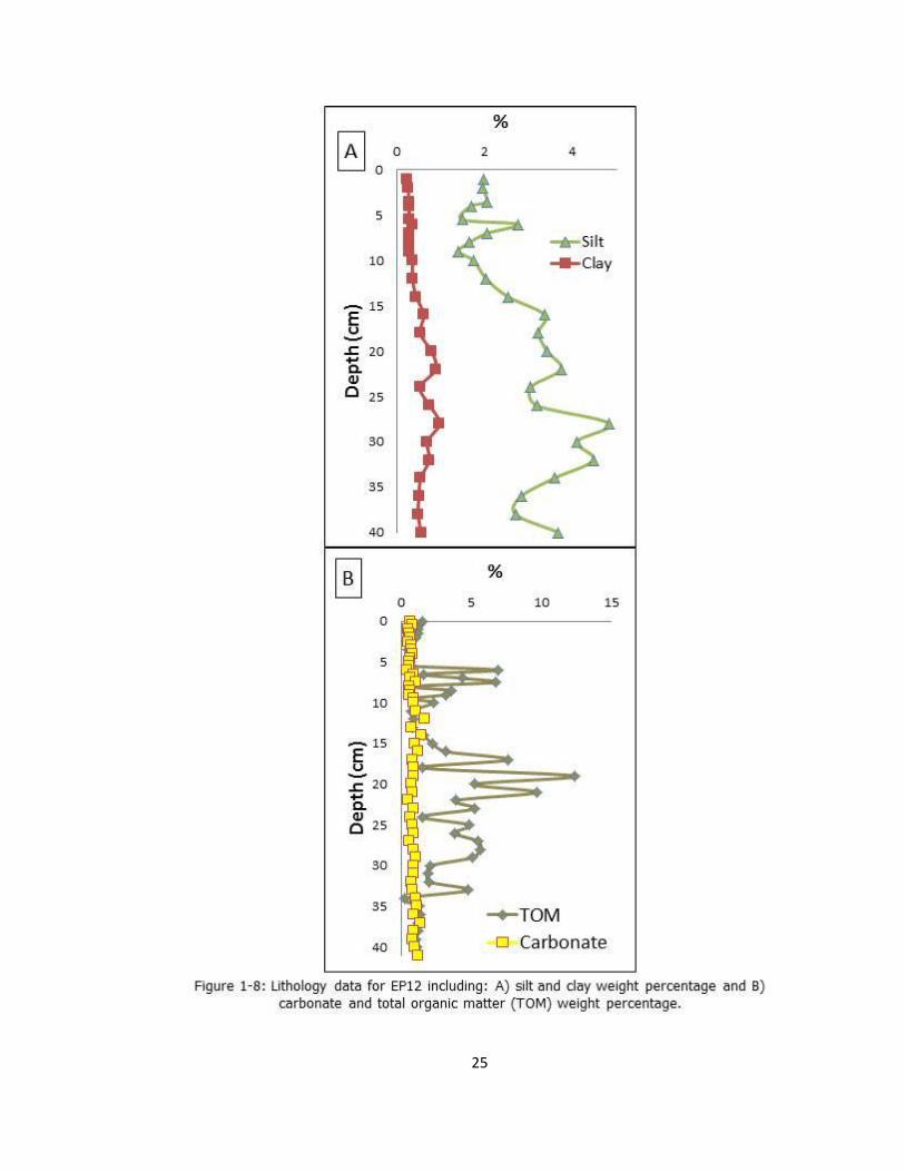
terrigenous, carbonate and organic (TOM) ............................................. 24 Figure 1-8: Lithology data for EP12 including: A) silt and clay weight percentage
and B) carbonate and total organic matter (TOM) weight percentage ....... 25 Figure 1-9: Graph of the 210Pb and 137Cs records along with the depth vs. date
curve based on the CRS model from EP12 ............................................. 27 Figure 1-10: Graph of the EP12 mass accumulation rates (MAR) including bulk,
terrigenous, carbonate and organic (TOM) ............................................. 28 Figure 1-11: Lithology data for EP15 including: A) silt and clay weight percentage
and B) carbonate and total organic matter (TOM) weight percentage ....... 30

vii
Figure 1-12: Graph of the 210Pb and 137Cs records along with the depth vs. date curve based on the CRS model from EP15 ............................................. 31
Figure 1-13: Graph of the EP15 mass accumulation rates (MAR) including bulk,
terrigenous, carbonate and organic (TOM) ............................................. 33 Figure 1-14: Lithology data for EP17 including: A) silt and clay weight percentage
and B) carbonate and total organic matter (TOM) weight percentage ....... 34 Figure 1-15: Graph of the 210Pb and 137Cs records along with the depth vs. date
curve based on the CRS model from EP17 ............................................. 36 Figure 1-16: Graph of the EP17 mass accumulation rates (MAR) including bulk,
terrigenous, carbonate and organic (TOM) ............................................. 37 Figure 1-17: Lithology data for EP18 including: A) silt and clay weight percentage
and B) carbonate and total organic matter (TOM) weight percentage ....... 39 Figure 1-18: Graph of the 210Pb and 137Cs records along with the depth vs. date
curve based on the CRS model from EP18 ............................................. 40 Figure 1-19: Graph of the EP18 mass accumulation rates (MAR) including bulk,
terrigenous, carbonate and organic (TOM) ............................................. 42 Figure 1-20: Lithology data for EP19 including: A) silt and clay weight percentage
and B) carbonate and total organic matter (TOM) weight percentage ....... 43 Figure 1-21: Graph of the 210Pb and 137Cs records along with the depth vs. date
curve based on the CRS model from EP19 ............................................. 45 Figure 1-22: Graph of the EP19 mass accumulation rates (MAR) including bulk,
terrigenous, carbonate and organic (TOM) ............................................. 46 Figure 2-1: Map of land use in the Manatee River Watershed as of 2007 showing
the urban development of Bradenton and Palmetto near the mouth of the river .......................................................................................... 52
Figure 2-2: Location map of Florida expanding to the location of the seven
selected core sites throughout the Manatee River with reference to the cities of Bradenton and Palmetto as well as the Manatee River Dam ................................................................................................... 58
Figure 2-3: The arsenic enrichment factor records for all five sites (EP9, 10, 12,
15, and 17) ......................................................................................... 62 Figure 2-4: (A) The copper enrichment factor records for all sites (EP9, 10, 12,
15, and 17) and (B) the copper enrichment factor records for all sites except EP10. ............................................................................... 64

viii
Figure 2-5: The lead enrichment factor records for all five sites (EP9, 10, 12, 15,
and 17) .............................................................................................. 66 Figure 2-6: Cartographic representations of heavy metal enrichment factors at
each site by decade. ............................................................................ 71 Figure 2-7: Median heavy metal concentration records from all sampling sites by
decade from 1910-2009 ....................................................................... 74 Figure 2-8: Manatee County agricultural acreage and integrated arsenic
enrichment history from 1900-2009 ...................................................... 76 Figure 2-9: Correlation of Manatee County agricultural acreage and the
integrated arsenic enrichment factor record from 1900-2009 ................... 76 Figure 2-10: Florida fuel consumption in billions of gallons and the integrated
lead enrichment record from 1945-1995 ................................................ 78 Figure 2-11: Correlation of Florida fuel consumption in billions of gallons and the
integrated lead enrichment record from 1945-1995 for the Manatee River. ................................................................................................. 78
Figure 2-12: A graph depicting the integrated copper enrichment values above
the mean occurring simultaneously with periods of persistent, heavy precipitation ........................................................................................ 80
Figure 3-1: Location map of Florida expanding to the location of the transect of
13 water sampling sites throughout the Manatee River with reference to the three instrumental records of temperature and salinity as well as the Manatee River Dam ............................................. 91
Figure 3-2: 210Pb and 137Cs records along with the CRS model dates from 1914-
2009 .................................................................................................. 95 Figure 3-3: Extrapolation of CRS model linear accumulation rate calculated from
sampling depths 18, 19 and 20 cm ........................................................ 96 Figure 3-4: Relationship between Mg/Ca(W) and measured salinity at each site for
February, March and August, 2010. ....................................................... 97 Figure 3-5: Foraminferal Mg/Ca and temperature ...................................................... 99 Figure 3-6: Temperature record for core EP17 with depth (A) and date (CE) (B). ....... 100 Figure 3-7: δ18O(C) and δ13C(C) values for hand-picked Ammonia sp. in the surficial
samples of core EP17 from each size fraction ....................................... 102

ix
Figure 3-8: δ13C(C) record from EP17 showing a gradual decrease throughout the record by depth (A) and date (B) ........................................................ 103
Figure 3-9: EP17 δ18O(C) record with depth (A) and date (B) ..................................... 105 Figure 3-10: EP17 δ18O(W)(VSMOW) record from 1550-2009 ..................................... 106 Figure 3-11: EP17 Mg/Ca(C) temperature and δ18O(W) records from 1550-2009
showing cooler periods with increased precipitation from 1652-1710 (LIA I) and then from 1855-1884 (LIA II) ............................................ 112

x
Abstract
The Manatee River Watershed (Manatee County, FL) has experienced heavy
anthropogenic development over the last 100 years and was relatively pristine previous
to this development. The population growth within the watershed has surpassed the
national trends and has doubled in the last 30 years. The heavy anthropogenic
development has led to depletion in natural resources, nutrient loading, coastal erosion,
and increased pollution. This study constructs records of sedimentological processes to
compare the pre-development records to the past 100 years of anthropogenic
development. The first portion of this study identifies specific changes in sedimentation
attributed to anthropogenic activity in the Manatee River. Anthropogenic development
has increased the input of terrigenous material into the river by as much as an order of
magnitude (0.3-3.0 g/cm2/yr) over three periods; 1) the predevelopment period (1900-
1941), 2) the agricultural development period (1941-1970’s), and 3) the urban
development period (1970’s-2010). The second portion of this study examines records
of heavy metal (As, Cu, Pb) enrichment in the Manatee River. There are areas in the
Manatee River that currently have, or recently have had, concentrations of heavy metals
above the EPA regional screening levels. Throughout all of the Manatee River sediment
cores there has been a continuous increase in the concentration of arsenic (0.32-20.91
ppm), lead (0.35-35.79 ppm) and copper (1.49-49.55 ppm) from 1900-2010. The third
portion of this study utilizes calcareous tests from benthic foraminifera (Ammonia
beccarii) in the longest sediment core to determine the Mg/Ca, 18O/ 16O, and 13C/ 12C

xi
ratios as proxies for river water temperature, salinity and nutrient content. These
proxies allow for the assessment of changes in rates and range of river water
parameters from the pre-anthropogenic to the anthropogenic periods. A Manatee River
temperature record, precipitation/evaporation record and nutrification record have been
constructed for the last 450 years (1550-2009 CE). These records are necessary to
inform and enhance future coastal resource management practices.

1
Introduction
As of the year 2003, more than half of the population of the United States lived within
fifty miles (80.5 km) of a coast (NOAA, 2011). Between 1980 and 2003, the coastal
population increased by 33 million residents. The expected continuation of this trend
makes it increasingly important to compile information necessary to inform and enhance
coastal resource management practices. Natural resources such as fisheries, beaches,
and access to clean water are immensely important to coastal economies.
This study focuses on the Manatee River, located on the west coast of Florida in the
southeastern portion of the Tampa Bay Estuary (Figure 1). The Manatee River
Watershed has experienced increasing anthropogenic development over the last 100
years and was relatively pristine previous to this development. The population growth
within the watershed has surpassed the national trends and has doubled in the last 30
years (Table 1). The heavy anthropogenic development has led to depletion in natural
resources, increased nutrient loading, coastal erosion, and increased pollution (Wilmore
and Pyrtle, 2004).

2
Figure 1: Location map of the Manatee River with reference to the state of Florida and the United
States.

3
One goal of the study is to understand natural processes in the watershed prior to the
period of anthropogenic development to assess how to better manage the extensively
developed watershed. This study seeks to construct records of sedimentological
processes and to compare the pre-development records to the past 100 years of
anthropogenic development. The transition between the natural (pristine) period and
the developed (anthropogenic) period has been recorded in the sediments of the
Manatee River. The records to be examined include: (1) the salinity and temperature of
the Manatee River based on proxy records in benthic foraminifera; (2) the
concentrations of heavy metal pollutants throughout the river; and (3) changes in the
types and amounts of sediment being introduced to the Manatee River, Tampa Bay, and
ultimately the Gulf of Mexico. These records will answer questions such as: (1) Has
anthropogenic development changed the temperature and/or salinity of the Manatee
River? (2) What are the baseline concentrations of heavy metals in the river and what
types of land-use have increased those concentrations? (3) Has anthropogenic
development introduced new types of sediments or increased the rates of
sedimentation? Constructing such records will clarify management goals based on the
pristine period in the watershed to better reconcile the needs of an increasing coastal
(human) population and the processes needed to maintain coastal resources.

4
Table 1: Manatee County population estimates and projections from 1980-2020 (SFWMD, 2001).
Population Estimates and Projections
Area 1980 1990 1995 2000 2010 2020
Manatee County 148,800 211,700 223,500 258,410 302,710 344,000
City of Bradenton 30,288 43,779 47,679 52,752 61,549 N/A
City of Palmetto 8,637 9,268 10,454 12,130 14,588 15,553

5
Chapter One
Determining anthropogenic effects on sedimentation in the Manatee River, Manatee
County, FL
Introduction
To assess the land use record and temperature and salinity records from a sediment
column in any environment, a basic understanding of the surrounding geologic setting, a
record of changes in lithology, and one or more geochronological tools are essential.
This chapter introduces the geologic setting of the Manatee River Watershed,
documents the recent changes in lithology of cores taken from Manatee River
sediments, and introduces the 210Pb dating method. The purpose of this chapter is to
identify specific changes in sedimentation, either rate or lithology, attributed to
anthropogenic activity in the Manatee River Watershed in the last century.
Geologic setting
Southwest Florida is built upon a carbonate platform with a surficial layer of carbonate
and siliceous sands and muds (McClellan and Eades, 1997). The surficial layer contains
Miocene phosphate deposits and has been subject to much phosphate-mining activity in
the last 100 years (Fairbridge, 1992; Gelsanliter et al., 1994). The Tampa Bay area is
located on the west-central portion of the Florida coastline and totals approximately
seven thousand square kilometers including estuarine waters, wetlands and drainage
basins. The bay is shallow with an average depth of 3.5 m and vegetation is dominated
by mangrove forest with some areas of salt marsh, both of which contribute a significant

6
portion of the organic matter in Tampa Bay sediment (Swarzenski and Yates, 2007).
The Manatee River begins in Manatee County, FL, southeast of Tampa Bay at an
elevation of 39.6 m and proceeds westward for 72.4 km. The river drains approximately
932.4 km2 into the southern region of Tampa Bay and ultimately into the Gulf of Mexico
(SWFWMD, 2001).
Tampa Bay formed as sea level rose, from about 6-10,000 years before present, filling in
a series of freshwater lakes (Brooks and Doyle, 1998). There are two major sources of
sedimentary input into the bay, marine sediments (CaCO3) carried by tidal currents from
the Gulf of Mexico and terrigenous sediments (fine-medium grain quartz sand) via fluvial
systems (Brooks and Doyle, 1998; Swarzensky and Yates, 2007). Moving inland, there
have been several studies of pollutant histories of upper sections of rivers, primarily
trying to establish the effects of damming and other water control construction
(Kuwabara et al., 2007). Only a few studies have utilized sediment to quantify effects of
land use on an estuary (Caffrey et al., 2002; He et al., 2006), including one in Charlotte
Harbor (Charlotte County, FL) which determined that the increase of nitrogen from the
expanding agricultural activity is greatly increasing the anoxic events that span 90 km2
of the Charlotte Harbor Estuary (Turner et al., 2006). This study will be the first to use
mass accumulation rates of specific constituents in the sediment to determine the effect
of anthropogenic development on the fluvial and estuarine environments of the Manatee
River.
Radionuclide background
Short-lived radioisotopes such as Cesium-137 (137Cs) and Lead-210 (210Pb) have been
used for many applications to produce corroborating geochronologies for the past 100
years (Eisenbud and Gessel, 1997; Pourchet et al., 2000; Robbins et al., 2000; Brenner

7
et al., 2001; Brenner et al., 2004; Suzuki et al., 2005; Harle et al., 2006; Baskaran and
Swarzenski, 2007). 210Pb is produced in the Uranium-238 (238U) decay series. This
series, by way of Thorium-230 (230Th) losing an alpha particle, initially produces Radium-
226 (226Ra), with a half-life of 1600 years, in terrigenous, freshwater, and marine
systems. The 226Ra present in surface rock disintegrates by alpha emission and diffuses
into the atmosphere becoming Radon-222 (222Rn) at a rate as high as ~42
atoms/minute/cm2 (Holmes, 2004). With a very short half-life of 3.8 days, 222Rn decays,
again by alpha emission, to Lead-214 (214Pb). Through beta emission, in a time scale of
minutes, Bismuth-214 (214Bi) is formed in the atmosphere and the daughter product of
214Bi through alpha emission is 210Pb. The atmospheric 210Pb then binds to particulate
matter in the atmosphere and falls into the sediment or water either by gravity or by
rain (Pourchet et al., 2000). Once deposited, 210Pb activity is not recharged, and thus
begins to decay at a constant rate. The half-life of 210Pb is 22.3 years, which ultimately
decays into Polonium-210 (210Po) and then through alpha emission, becomes the stable
isotope of Lead-206 (206Pb).
210Pb is produced in situ in each drainage basin. This 210Pb is referred to as supported
210Pb (Noller, 2000). The 210Pb delivered by wet deposition into the watershed is
referred to as unsupported or excess 210Pb because it was not the daughter product of in
situ 226Ra (Noller, 2000). The excess 210Pb value is the difference between the total
210Pb (measured) and the supported 210Pb (calculated). 210Pb activity of a given aliquot
of sediment diminishes at a known decay rate as 210Pb decays to a 210Po until it reaches
the level of the supported 210Pb (background). The half-life for 210Pb is 22.3 years, and
because current technology can only trace 5-6 half-lives before the activity becomes too

8
small to trace with any accuracy, 210Pb geochronology is a robust tool for dating a
geologic column up to 120 years before the present (YBP).
As with any geochronological tool, excess 210Pb dating must be corroborated. This is
most effectively accomplished by using 137Cs, which is only produced in large quantities
during an atomic explosion (Livingston and Povinec, 2000). When 137Cs is released into
the atmosphere, global wind circulation distributes it worldwide and is deposited into the
sediment primarily through wet deposition (Aarkrog, 2003). In surface sediments, a
137Cs activity peak is found worldwide at about 1963, due to the atmospheric nuclear
tests being performed from the 1950’s to 1964, when the international atmospheric
nuclear test ban treaty took effect (Holmes, 2004). There are some regional exceptions
such as Chernobyl (1986), the latest Indian and Pakistani testing (1998), and the
Fukushima nuclear meltdown (2011), but none of these smaller events are expected to
be seen in the sediments of the Manatee River. The validation of the geochronology is
determined by how closely the 1963 137Cs peak corroborates the 210Pb date at the same
depth.
Radionuclide dating applications in Florida
210Pb has been shown to be a successful tool to date sediment columns as a tracer for
sediment dynamics in both marine/coastal and lacustrine/watershed settings. Sediment
accumulation rates are quite variable throughout Florida. Florida Bay has the highest
accumulation rate of 0.33-5.8 cm/yr (Holmes et al., 2001). The river-dominated areas
(Steinhatchee, Charlotte Harbor, Saint Johns River Basin) have very similar accumulation
rates with 0.14 cm/yr, 0.25-0.28 cm/yr, and 0.33 cm/yr, respectively (Turner et al.,
2006, Brenner et al., 2001, Trimble et al., 1999). Brenner et al., (2001) found that the
sedimentation rate increased between 1.7-3.4-fold in the Saint Johns River Basin (SJRB)

9
between pre-anthropogenic and anthropogenic times. These changes are attributed to
modifications in the hydrology of the fluvial system as well as to urban sources of
organic nutrients.
Sedimentation rate in Lake Okeechobee tends to be intermediate at 0.78 cm/yr and the
lowest accumulation rate was reported in Rookery Bay at 0.14-0.17 cm/yr (Lynch et al.,
1989; Brezonik and Engstrom, 1998). Across a suite of cores in Lake Okeechobee,
Brezonik and Engstrom (1998) calculated that there had been a two-fold increase in
sediment accumulation rate (3-6 g/cm2/yr) and a four-fold increase in the rate of total
phosphorus deposition in Lake Okeechobee since the early 1900’s.
There are a few limitations to utilizing 210Pb geochronology in Florida. The high activities
of 226Ra in the groundwater combined with the very porous bedrock and karst terrain
make it difficult to find reliable inland sampling sites that provide enough excess 210Pb to
date the sediment (Holmes et al., 2001). 137Cs can be deposited initially well after its
release into the atmosphere due to potentially long residence times in the atmosphere
(years), which can affect its use as a corroborative geochronological tool. By sampling
both sediments and corals from the Florida Bay area, Robbins et al. (2000) have shown
that there is a lag in the time that atmospheric radionuclides are formed and the time
they are deposited. This is a significant finding in that it affects the age calculation in
sediments which is based on the initial concentration at time of deposition. In other
words, if a 137Cs record is being used to corroborate a 210Pb record and that 137Cs was
assumed to have been deposited in 1963 when it was really deposited in 1970, then the
corroborative tool is not functional. The final limitation that must be addressed when
selecting a sampling site is the competition of organic matter for binding sites on
sediment particles. Binford and Brenner (1986) demonstrate that radionuclide activities

10
are inversely related to the total amount of organic matter in Florida lakes. This inverse
relationship has to do with the fact that organic matter competes with radionuclides for
binding sites on fine-grained sediment particles. By taking these limitations into
account, 210Pb geochronology can be a robust tool to determine sedimentation rates,
sediment dynamics, and pollution histories over the last 100 years in the marine,
coastal, watershed, and lacustrine environments of Florida.
Methods
Sampling methods
Seven sediment cores were collected throughout the Manatee (Figure 1-1). The core
sites were selected by locating areas with little potential for resuspension and medium-
to-fine-grained sediment. These cores were taken by a diver-assisted push-coring
method with 3-1/2” diameter acrylic barrel. Push cores provide a short-term
environmental development record (hundreds to thousands of years before present).
Sub-samples of each core were taken by an extrusion method. To do so, the core was
placed upon an extrusion device with a plunger the same diameter as the inner rim of
the core barrel and a threaded piston calibrated to one turn per centimeter. The
sediment was extruded at 0.5 cm (0-10 cm) and at 1.0 cm for the remainder of each
core. Samples were kept in plastic bags and frozen. The frozen samples were then
freeze dried.

11

12
Sedimentology laboratory methods
Approximately 5 grams of each sediment sample were sieved at 63 µm. Silt and clay
weight percentages (fine fraction) were determined by using a Saturn DigiSizer High
Resolution Laser Particle Size Analyzer at the University of South Florida (USF), College
of Marine Science. A manual pipetting method developed by Folk (1965) was also used
on certain samples to determine any errors in the DigiSizer measurement. It is assumed
that the coarse fraction (sand and gravel) weight percentage is the difference between
the fine fraction and 100% and is therefore not reported. The percentage of each grain
size aids in determining the depositional environment, as well as identifying land use
signatures.
Loss on ignition (LOI) analysis was run on the samples to determine the total organic
matter and percent carbonate material for determination of depositional environment
(Milliman, 1974; Dean, 1974; Heiri et al., 2001). Approximately one gram of each
sample was placed into a crucible and ignited at 550 0C in a muffle furnace for 4 hours
and the percent total organic matter (TOM) was determined by the mass difference after
ignition. The remainder was then placed back into the muffle furnace and ignited at 950
oC for 1.5 hours and the percent carbonate (CO3) content was determined by mass
difference (Dean, 1974).
Radionuclide laboratory methods
A Canberra planar high purity germanium (HPGe) detector was used to determine 210Pb
and 137Cs activity throughout each core at the USF College of Marine Science. For planar
gamma detection, samples were freeze-dried and placed in vacuum-sealed aluminum
cannisters. Once sealed, the samples were allowed to achieve secular equilibrium for 28
days. The samples were then counted for 24-48 hours based on sample size. Reported
13
error is the product of the net uncertainty from the detector and the standard deviation
of the excess 210Pb record for each core.
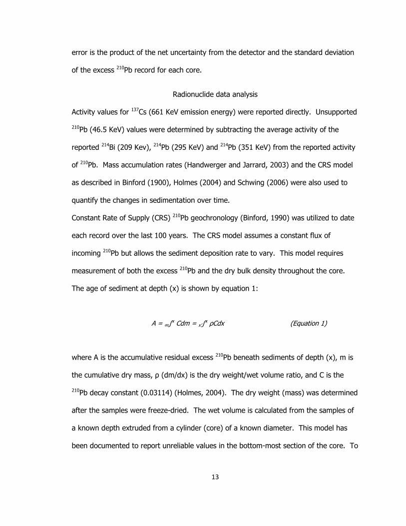
Radionuclide data analysis
Activity values for 137Cs (661 KeV emission energy) were reported directly. Unsupported
210Pb (46.5 KeV) values were determined by subtracting the average activity of the
reported 214Bi (209 Kev), 214Pb (295 KeV) and 214Pb (351 KeV) from the reported activity
of 210Pb. Mass accumulation rates (Handwerger and Jarrard, 2003) and the CRS model
as described in Binford (1900), Holmes (2004) and Schwing (2006) were also used to
quantify the changes in sedimentation over time.
Constant Rate of Supply (CRS) 210Pb geochronology (Binford, 1990) was utilized to date
each record over the last 100 years. The CRS model assumes a constant flux of
incoming 210Pb but allows the sediment deposition rate to vary. This model requires
measurement of both the excess 210Pb and the dry bulk density throughout the core.
The age of sediment at depth (x) is shown by equation 1:
A = ∞∫x Cdm = x’∫x ρCdx (Equation 1)
where A is the accumulative residual excess 210Pb beneath sediments of depth (x), m is
the cumulative dry mass, ρ (dm/dx) is the dry weight/wet volume ratio, and C is the
210Pb decay constant (0.03114) (Holmes, 2004). The dry weight (mass) was determined
after the samples were freeze-dried. The wet volume is calculated from the samples of
a known depth extruded from a cylinder (core) of a known diameter. This model has
been documented to report unreliable values in the bottom-most section of the core. To

14
avoid unreliable dates at the bottom of each record, dates calculated before the year
1900 were not reported.
Mass accumulation rates are the product of the bulk density of each sample and the
linear accumulation rate (LAR). Mass accumulation rates quantify the amount of bulk
sediment and constituent (terrigenous, carbonate, and TOM) material accumulating
throughout each sediment record (Handwerger and Jarrard, 2003) and account for any
compaction in the sediment column. The dry bulk density (DBD) and constituent
densities (CD) needed to calculate mass accumulation rate are calculated using
equations 2 and 3. These densities are based on the known volume of each sample
during the extrusion of the core and the measured dry mass after being freeze-dried.
DBD (g/cm3) = dry mass (g) / (sample vol (cm3) (Equation 2)
CD (g/cm3) = const. mass (g) / (sample vol (cm3) (Equation 3)
Linear accumulation rates were calculated by the following:
LAR = z/(Ds - DCRS ) (Equation 4)
where LAR is the linear accumulation rate, Ds is the sampling date, DCRS is the CRS date
for the given sample, and z is the sample depth. An average linear accumulation rate
was calculated for each core by averaging the linear accumulation rate for every sample
in the core.
Results
The lithology, radionuclide, and mass accumulation rate records of the seven push-cores
collected from throughout the Manatee River are described below (Table 1-1). Each
represents a record from a different sampling environment and sedimentological
response to natural and anthropogenic events. Criteria for selecting coring sites

15
included fine-grain surface sediment for highest possible radionuclide activity and areas
likely to have the least resuspension due to tidal or river energy.
Table 1-1: Sampling site information including core name, recovery length, location and water depth.
Core Name Recovery (cm) Latitude Longitude Water Depth (m)
EP-07-PC-09 24 27.52947 82.62617 1.3
EP-07-PC-10 31 27.53257 82.64657 2.1
EP-07-PC-12 41 27.53264 82.64282 2.7
EP-08-PC-15 35 27.53382 82.63708 1.1
EP-08-PC-17 46 27.50892 82.59028 4.5
EP-10-PC-18 42 27.4979 82.52267 2.6
EP-10-PC-19 43 27.51932 82.48901 2.4
Core EP-07-PC-09
Core EP-07-PC-09 (EP9) was collected in an estuarine environment near the mouth of
the Manatee River (27.52947o N, 82.62617o W) just south (riverward) of Snead Island
and a large oyster (Crassostraea virginica) bed. The recovered sediment column was 24
cm in length.
Lithology
The base of EP9 is silty-sand with abundant small shell fragments. Moving upcore, there
are fine-grained (silt) layers at 20 cm and 12 cm depth along with decreasing carbonate
material from the base of the core to 7.5 cm depth (Figure 1-2). As the carbonate
material decreases up-core, a fining upward sequence (increasing silt and clay) occurs
from 10 cm to 4.5 cm. A sudden increase in grain size (sand) occurs at 4cm and
another, smaller fining upward sequence terminates at the top of the core (3.5 cm to 0
cm). There is also a decrease in organic material from 11 cm to 7.5 cm, which is
synchronous with the most dramatic decrease in carbonate material.

16

17
Radionuclide Analysis
The excess 210Pb record from EP9 shows the gradual increase from background activity
at 23 cm up-core as expected (0-22.4 dpm/g), with several periods of low activity (9-12
cm and 5-7 cm) (Figure 1-3). The 137Cs record shows peaks from 16 cm to 11cm (1956-
1964) and a few smaller peaks up core at 5.5 cm to 4.5 cm and 1.5 cm to 0.5 cm. The
results from the CRS model show an initial slope of accumulation with a linear
accumulation rate (LAR) of 0.22 cm/yr from the base of the core to 20 cm (1906-1941).
This slope increases (increased accumulation) to a LAR of 0.31 cm/yr from 20 cm to 9.5
cm (1941-1967) and is followed by a rapid decrease in slope from 9 cm to 7.5 cm.
The slope steepens again from 7.5 cm to 5 cm (1976-1982). There is a low slope from
5 cm to 1 cm (1982-2005) with an LAR of 0.17 cm/yr. The average LAR for the entire
core is 0.25 cm/yr.
Mass Accumulation Rates
The mass accumulation rate (MAR) record from EP9 shows episodic pulses of both
terrigenous and carbonate material in 1941, 1956, and 2005 along with a large,
continuous increase in both constituents from 1968-1979 (Figure 1-4). The bulk
accumulation rate is almost entirely composed of terrigenous material seeing as both are
within 0.2-1.0 g/cm2/yr and covary with each other throughout the entirety of the core.
The accumulation rates of carbonate (CaCO3) and organic matter (TOM) are an order of
magnitude lower between 0-0.07 g/cm2/yr.

18
Figure 1-3: Graph of the 210Pb and 137Cs records along with the depth vs. date curve based on
the CRS model from EP9.
2007 2006 2005
2000 1996
1993 1989
1987 1984
1982 1979 1979 1978 1978 1977 1976
1972 1968 1968 1967
1964 1962 1961
1959 1958
1956 1951
1948 1945
1941 1933
1924 1915
1906
0 10 20 30
0
5
10
15
20
De
pth
(cm
)
Activity (dpm/g)
CRS Date
Cs-137
Pb-210

19
Figure 1-4: Graph of the EP9 mass accumulation rates (MAR) including bulk, terrigenous,
carbonate and organic (TOM). (Note the change in scale on the x-axes).
0 0.02 0.04 0.06 0.08
1900
1920
1940
1960
1980
2000
0 0.5 1
Year
Bulk & Terrigenous g/cm^2/yr
Bulk
Terrigenous
CO3
TOM
TOM & CO3 g/cm^2/yr

20
Core EP-07-PC-10
Core EP-07-PC-10 (EP10) represents the most seaward sampling site and was collected
in an open estuarine environment west (seaward) of Emerson Point just outside the
mouth of the Manatee River (27.53257o N, 82.64657o W). The recovered sediment
column was 31 cm in length.
Lithology
EP10 is primarily fine-to-medium-grained quartz sand throughout, with small increases
in fine grains (silt) at 22 cm, 16 cm to 14 cm, and 8 cm and almost no clay-size particles
(Figure 1-5). There is also a coarsening upward trend throughout the entire core.
There is also very little carbonate and organic matter throughout the core. There is an
increase in carbonate material from 12 cm to 5.5 cm up-core followed by a decrease
from 5.5 cm to the surface.
Radionuclide Analysis
The 210Pb record from EP10 gradually increases from background at 28 cm to the
surface of the core (0-26.6 dpm/g) (Figure 1-6). There is, however, a large depletion in
activity from 18 cm to 14 cm. The 137Cs record shows the earliest activity at 20 cm and
subsequent activity more recently at 12, 9, 7, and 2 cm. The earliest activity in this core
is corroborated by the CRS model and occurs at some point between 1958 and 1970.
There are two main periods according to the CRS model. The first occurs from the base
of the core to 20 cm depth (1904-1970) with a LAR of 0.23 cm/yr. At that point, there
is a large increase in slope throughout the rest of the core from 20 cm to the surface of
the core (1970-2009) with a LAR as high as 0.89 cm/yr. The average LAR for the entire
core is 0.58 cm/yr.

21

22
Figure 1-6: Graph of the 210Pb and 137Cs records along with the depth vs. date curve based on
the CRS model from EP10.
2007 2006 2006
2005 2003 2003 2002
2001 1999 1998 1997 1997 1996 1996 1995 1995 1995 1995 1994
1993 1992
1989 1986
1983 1979
1977 1977 1976 1975
1973 1970
1958 1945
1939 1930
1923 1919
1911 1904
0 10 20 30
0
5
10
15
20
25
30
De
pth
(cm
)
Activity (dpm/g)
CRS Date
Cs-137
Pb-210

23
Mass Accumulation Rates
The bulk accumulation rate from EP10 is also dominated by terrigenous material
showing a parallel trend throughout the core from 0.00-1.60 g/cm2/yr (Figure 1-7). The
carbonate and organic accumulation rates range between 0.00-0.16 g/cm2/yr. All of the
accumulation rates are relatively constant throughout the bottom of the core (1903-
1969). The surface section of the core is marked by three features: 1) a small increase
in terrigenous and carbonate material from 1969-1983, 2) a large increase in all
constituents from 1989-1996, and 3) a gradual increase towards the surface of the core
in carbonate and terrigenous material from 2002-2007.
Core EP-07-PC-12
Core EP-07-PC-12 (EP12) was collected just landward of the mouth of the Manatee
River, just southeast of Emerson Point (27.53264o N, 82.64282o W). The sampling
environment was restricted estuarine adjacent to a growth of black mangroves
(Avicennia germinans) to the north. The recovered sediment column was 41 cm in
length.
Lithology
EP12 is primarily fine-grained sand throughout the entire core [<5% mud (silt and
clay)]. There is a coarsening upward trend throughout the core with increased fine-
grained (silt) particles at 32 cm to 28 cm, 22 cm to 16 cm, 6 cm, and at the surface
(Figure 1-8). There is a significant amount of organic material in EP12, with an increase
up-core from 35 cm to 18 cm, a rapid decrease from 18 cm to 15cm, and another
smaller increase from 11cm to 6 cm. A layer of small shell fragments is also present
from 16 cm to 11 cm. Much like EP10, EP12 exhibits a coarsening upward sequence.

24
Figure 1-7: Graph of the EP10 mass accumulation rates (MAR) including bulk, terrigenous,
carbonate and organic (TOM). (Note the order of magnitude change in scale on the x-axes).
0.00 0.05 0.10 0.15 0.20
1900
1920
1940
1960
1980
2000
0 0.5 1 1.5 2
Year
Bulk & Terrigenous g/cm^2/yr
Bulk
Terrigenous
CO3
TOM
TOM & CO3 g/cm^2/yr
25

26
Radionuclide Analysis
The 210Pb activity in EP12 increases from background at 20 cm to the surface (0-22.6
dpm/g) with very few excursions (Figure 1-9). There is a small excursion (depletion)
from 4 cm to 2 cm and is synchronous with increased 137Cs activity from 5 cm to 2 cm
(2000-2002). The 137Cs record shows small activity values at 16 cm and 14 cm (1941
and 1952 respectively) and a large peak between 12 cm and 10 cm (1963-1979). The
CRS model shows three main periods of accumulation. The first is from 16-18 cm where
there is a relatively shallow slope (low accumulation), followed by a period of increased
accumulation from 16 cm to 10 cm (1941-1979), much like EP9. The third main period
of accumulation is from 10 cm to the surface (1979-2009) with an exponentially
increasing slope and a slight decrease at 2 cm (2004).
Mass Accumulation Rates
The relationship between terrigenous and bulk accumulation rates is much like that of
EP9 and 10 and range between 0.19-1.12 g/cm2/yr (Figure 1-10). The carbonate
accumulation rates are more than two orders of magnitude lower than terrigenous,
while the TOM accumulation rate is much higher (0.004-0.07 g/cm2/yr) than the
carbonate MAR (0.003-0.010 g/cm2/yr), unlike in EP9 and EP10. Moving up-core from
1970-1998, the terrigenous and organic MAR roughly triple and then decrease slightly
from 1998-2003, where they both begin to increase again from 2003-2007.

27
Figure 1-9: Graph of the 210Pb and 137Cs records along with the depth vs. date curve based on
the CRS model from EP12.
2007 2006 2006
2004 2002 2002 2001 2002 2002 2001 2000 1999 1998
1996 1995
1993 1991
1989 1986
1982 1979
1971
1963
1958
1952
1947
1941
1925
1909
1907
1905
0 10 20 30
0
2
4
6
8
10
12
14
16
18
20
De
pth
(cm
)
Activity (dpm/g)
CRS Date
Cs-137
Pb-210

28
Figure 1-10: Graph of the EP12 mass accumulation rates (MAR) including bulk, terrigenous,
carbonate and organic (TOM). (Note the change in scale on the x-axes).
0 0.02 0.04 0.06 0.08
1900
1920
1940
1960
1980
2000
0 0.5 1 1.5
Year
Bulk & Terrigenous g/cm^2/yr
Bulk
Terrigenous
CO3
TOM
TOM & CO3 g/cm^2/yr

29
Core EP-08-PC-15
Core EP-08-PC-15 (EP15) was collected in a red mangrove (Rhizophora mangle) lagoon
east of Emerson Point (27.53382o N, 82.63708o W). The recovered sediment column
was 35 cm in length.
Lithology
The base of EP15 is well-sorted, silty-sand with a few small increases in finer grained
(silt) particles at 30 cm to 28 cm and 26 cm to 24 cm (Figure 1-11). At 14 cm there is a
large and abrupt fining upward sequence to the surface of the core. Similarly, there is
very little carbonate or organic matter at the base of the core, but at 14 cm, both begin
to increase up-core. At 7 cm, there is a step-wise increase in carbonate material.
Radionuclide Analysis
The 210Pb record for EP15 gradually increases from background at 19 cm to the surface
(0-27.4 dpm/g) as expected with only one positive excursion from 6 cm to 5 cm (32.8
dpm/g) (Figure 1-12). The 137Cs record has increased activity from 10 cm to 7 cm with
the largest peak at 9 cm (1960) and only a few small increases upcore at 4 cm and 2
cm. There is good age agreement between the 137Cs and 210Pb records. The CRS model
shows three periods of accumulation. The first period is from 19cm to 16 cm (1904-
1925) with a LAR of 0.17 cm/yr and gradually increases from 16cm to 6 cm (1925-1982)
with a LAR of 0.19 cm/yr. The third and final period occurs from 6 cm to the surface
(1982-2008) with a LAR of up to 0.52 cm/yr. The average LAR for the entire core is
0.24 cm/yr.

30

31
Figure 1-12: Graph of the 210Pb and 137Cs records along with the depth vs. date curve based on
the CRS model from EP15.
2008 2007 2006
2004 2002
1999 1996 1995 1993
1992 1991
1986 1982
1977 1972
1970 1968
1964 1960
1958 1955
1950
1944
1939
1934
1930
1925
1916
1904
1901
0 10 20 30 40
0
2
4
6
8
10
12
14
16
18
20
De
pth
(cm
)
Activity (dpm/g)
CRS Date
Cs-137
Pb-210

32
Mass Accumulation Rates
The terrigenous accumulation rate (0.50 g/cm2/yr) dominates the bottom half of the
record from 1900-1955, when it begins to decrease and the organic MAR begins to
increase (0-1.20 g/cm2/yr) throughout the upper section of the core from 1955-2008
(Figure 1-13). Carbonate matter also begins to increase in the upper section of the core
from 1970-2008 (0-0.28 g/cm2/yr).
Core EP-08-PC-17
Core EP-08-PC-17 (EP17) was collected in the central portion of the Manatee River in an
estuarine environment (27.50892o N, 82.59028o W). The recovered sediment column
was 46 cm in length.
Lithology
Working up-core from the silty-sand base with some organic material, there are two
finer grained layers with increased organic material at 42 cm and 34 cm (Figure 1-14).
There is a gradual coarsening upward sequence from 46 cm to 16 cm. The organic
material also decreases gradually over this section. Directly above the fining upward
sequence, there is both an abrupt decrease in organic matter and an increase in grain
size (sand) from 15 cm to 10 cm. Carbonate material is relatively constant throughout
the bottom of the core and then gradually decreases at this interval as well. The
sediment in the surface section (10 cm to the surface) is slightly finer than the 15 cm to
10 cm section, and contains a gradual decrease in organic matter and a rapid decrease
in carbonate material.

33
Figure 1-13: Graph of the EP15 mass accumulation rates (MAR) including bulk, terrigenous,
carbonate, and organic (TOM). (Note the change in scale on the x-axes).
0 0.5 1 1.5
1900
1920
1940
1960
1980
2000
0 0.5 1 1.5
Year
Bulk & Terrigenous g/cm^2/yr
Bulk
Terrigenous
CO3
TOM
TOM & CO3 g/cm^2/yr

34

35
Radionuclide Analysis
The 210Pb record from EP17 increases from background at 20 cm to the surface (0-8.87
dpm/g) with a depletion of activity in the surficial unit (5 cm to the surface) (Figure 1-
15). The 137Cs record shows increased activity over the 16 cm to 12 cm interval, which
corresponds to 1955-1972 in the CRS model. This corroborates the 210Pb record, despite
the depletion at the surface. The CRS model shows only two main periods of
accumulation at this site. The first is from 20 cm to 18 cm (1914-1943) with a LAR of
0.21 cm/yr. Then, from 18 cm to the surface (1943-2009) the slope steepens,
increasing to the surface with a LAR as high as 1.5 cm/yr. The average LAR for the
entire core is 0.50 cm/yr.
Mass Accumulation Rates
EP17 has the highest terrigenous MAR of any of the cores (0.84-4.10 g/cm2/yr) which is
fairly constant throughout the bottom of the core (1928-1975), decreasing slightly
between 1975 and 1981 and then increasing throughout the surface section of the core
(1981-2009) (Figure 1-16). The carbonate and TOM MAR’s both increase from the
bottom of the core (0.08-0.14 g/cm2/yr and 0-0.05 g/cm2/yr respectively) and then
gradually decrease from 1958-1981. They both increase along with the terrigenous MAR
from 1981-2009. Terrigenous input to this site has increased three-fold over the last
100 years.

36
Figure 1-15: Graph of the 210Pb and 137Cs records along with the depth vs. date curve based on
the CRS model from EP17.
2009 2009 2008 2007 2006 2006 2005
2003 2002 2001 2000
1998 1996
1993 1990
1989 1987
1985 1983
1981 1979
1976
1972
1967
1961
1958
1955
1949
1943
1929
1914
0 5 10
0
2
4
6
8
10
12
14
16
18
20
De
pth
(cm
)
Activity (dpm/g)
CRS Date
Cs-137
Pb-210

37
Figure 1-16: Graph of the EP17 mass accumulation rates (MAR) including bulk, terrigenous,
carbonate and organic (TOM). (Note the change in scale on the x-axes).
0 0.05 0.1 0.15
1900
1920
1940
1960
1980
2000
0 2 4 6
Year
Bulk & Terrigenous g/cm^2/yr
Bulk
Terrigenous
CO3
TOM
TOM & CO3 g/cm^2/yr

38
Core EP-10-PC-18
Core EP-10-PC-18 (EP18) was collected at the junction of the Braden River and the
Manatee River, in an estuarine environment near a black mangrove (Avicennia
germinans) stand and several shoal grass (Halodule wrightii) beds (27.4979o N,
82.52267o W). The recovered sediment column recovered was 42 cm in length.
Lithology
Throughout EP18, the dominant sediment constituent is medium-fine quartz sand, which
is expected, considering the core is one of the most landward of the sampling sites
(Figure 1-17). The percent silt fluctuates between 1-9% throughout the core. The only
definitive feature is a coarser layer at 26 cm with decreased fine grains (coarser) and
increased organic matter. Another thing to note are the shell fragments (increased
carbonate) at 38 cm and 34 cm.
Radionuclide Analysis
The 210Pb record from EP18 is the most consistent and increases from background at 16
cm to the surface (0-9.11 dpm/g) with no major excursions (Figure 1-18). The 137Cs
record also follows exactly what is expected in that there are decreasingly large peaks in
activity from 11 cm to 7.5 cm (1962-1986) and two small increases in activity towards
the surface at 3 cm and 1 cm. The CRS model for this core shows a gradual increase in
slope throughout the core with LAR at the base (15 cm) of 0.14 cm/yr and 1.23 cm/yr at
the surface (0.5 cm). This represents an order of magnitude increase in sedimentation
rate over the last one hundred years. The average LAR for the entire core is 0.40
cm/yr.

39

40
Figure 1-18: Graph of the 210Pb and 137Cs records along with the depth vs. date curve based on
the CRS model from EP18.
2010 2010 2009 2008 2007
2005 2003
2002 2000
1998 1997
1995 1992
1991 1990
1988 1986
1982 1979
1976 1973
1962
1951
1940
1929
1912
0 5 10 15
0
2
4
6
8
10
12
14
16
De
pth
(cm
)
Activity (dpm/g)
CRS Date
Cs-137
Pb-210

41
Mass Accumulation Rates
The MAR record from EP18 shows a gradual increase in all three main sedimentary
constituents with terrigenous material ranging from 0.30-3.17 g/cm2/yr, carbonate
material from 0-0.02 g/cm2/yr and organic matter from 0-0.03 g/cm2/yr (Figure 1-19).
All three begin to increase between 1961 and 1972. Slightly more organic matter
accumulated between 1992 and 1997. Terrigenous input has increased in this area by
an order of magnitude over the last one hundred years.
Core EP-10-PC-19
Core EP-10-PC-19 (EP19) represents the most landward site and was taken just seaward
(west) of the fluvial channels below the Manatee River Dam in a mixed estuarine/fluvial
environment surrounded by shoal grass (Halodule wrightii) beds. The recovered
sediment column was 43 cm in length.
Lithology
The entirety of EP19 is primarily medium-fine quartz sand. There is a coarsening
upward sequence from the base of the core to 22 cm (Figure 1-20). There is then a
rapid fining-upward sequence from 22 cm to 14 cm followed by another more subtle
coarsening-upward sequence from 14 cm to 10 cm. The surficial unit of EP19 is fairly
constant with respect to lithology (10 cm to the surface). Near the base of the core,
there is a peak in percent organic matter from 45 cm to 36 cm and another peak in
percent organic matter from 27 cm to 23 cm. Even in this core, being the farthest
landward extent of the sediment core transect, there is evidently a coarsening-upward
sequence throughout the core. This follows the same trend as many of the seaward
sampling sites.

42
Figure 1-19: Graph of the EP18 mass accumulation rates (MAR) including bulk, terrigenous,
carbonate and organic (TOM). (Note the two order of magnitude change in scale on the x-axes).
0 0.01 0.02
1900
1920
1940
1960
1980
2000
0 1 2
Year
Bulk & Terrigenous g/cm^2/yr
Bulk
Terrigenous
CO3
TOM
TOM & CO3 g/cm^2/yr

43

44
Radionuclide Analysis
The 210Pb record for EP19 increases from background at 16 cm to the surface (0-5.03
dpm/g) with only one significant excursion at 1 cm, which is also synchronous with an
increase in 137Cs (Figure 1-21). The 137Cs record has high activity peaks from 10 cm to 6
cm (1958-1988) with the highest activity at 9 cm (1964). This shows good age
agreement between the CRS model and the 137Cs record. The CRS model shows two
primary periods with the first occurring from 8-16 cm (1904-1973) and a LAR of 0.15
cm/yr. The second period is from 0-8 cm (1973-2010) with a LAR as high as 0.38
cm/yr. The average LAR for the entire core is 0.24 cm/yr.
Mass Accumulation Rates
The MAR records in EP19 shows a relatively constant input of organic and carbonate
material (0-0.01 g/cm2/yr and 0-0.05 g/cm2/yr, respectively) (Figure 1-22). However
there is a steady increase in terrigenous accumulation rate upcore (0.38-1.29 g/cm2/yr)
resulting in an increase in accumulation rate of more than four-times the rate in 1915.

45
Figure 1-21: Graph of the 210Pb and 137Cs records along with the depth vs. date curve based on
the CRS model from EP19.
2010 2008 2006 2005 2005
2002 2000
1998 1996
1994 1992
1990 1988
1985 1982
1977 1973
1968 1964
1961 1958
1952
1946
1937
1928
1916
1904
0 2 4 6 8
0
2
4
6
8
10
12
14
16
De
pth
(cm
)
Activity (dpm/g)
CRS Date
Cs-137
Pb-210

46
Figure 1-22: Graph of the EP19 mass accumulation rates (MAR) including bulk, terrigenous,
carbonate and organic (TOM). (Note the change in scale on the x-axes).
0 0.02 0.04 0.06
1900
1920
1940
1960
1980
2000
0 0.5 1 1.5
Year
Bulk & Terrigenous g/cm^2/yr
Bulk
Terrigenous
CO3
TOM
TOM & CO3 g/cm^2/yr

47
Discussion
The lithology and grain-size distribution (sediment texture) of each core, constrained by
short-lived radioisotope dating, yield records of natural events and anthropogenic events
as well as an overall environmental progression throughout the river. In many of the
cores and particularly EP17 and EP19, there were events characterized by increases in
fine particles and organic matter that are likely due to periods of increased precipitation
washing these materials downriver. Several of the cores also provide records of
anthropogenic events such as the construction of the Manatee River Dam (late 1960’s),
which is characterized by a layer of coarse quartz grains with increased carbonate
material and little to no organic material present (EP9 and EP17), as well as the
construction of the I-75 (1980) and US301 (1957) bridges across the river. There are
changes in the lithology and sediment texture that can be attributed to anthropogenic
activity such as the construction of a jetty near site EP9, which caused the deposition of
finer-grain sediment (baffling effect) and potentially the demise of the nearby oyster bed
(decrease in carbonate). Another event documented in the lithological record is the
clear-cutting of mangroves (less TOC) at site EP12 with the growth of agricultural
development. The overall progression of the lithology and texture in all of the cores is
primarily a coarsening upward sequence as the tidal energy increases throughout the
river and more anthropogenic development has introduced more, coarse, terrigenous
sediments (EP10, EP12, EP17, and EP19). The entire record shows a progression of the
river from dominantly fluvial to estuarine environments.
The radionuclide records provide a reliable geochronology for the upper extent of each
core on which to interpret the changes in sedimentation rate and type. The
corroboration between the 137Cs and the 210Pb-based CRS model in all cores supports the

48
accuracy of the age models. The radionuclide records themselves also help characterize
the anthropogenic influence on sedimentation. In every core, the surficial unit had
depletion in 210Pb activity synchronous with an increase in 137Cs, which can be attributed
to resedimentation from elsewhere in the watershed. These resedimentation periods
are primarily due to increased terrigenous material introduced by anthropogenic
development such as the construction of the I-75 bridge at EP17 (9 cm), a jetty near
site EP9 (7 cm to 5 cm), the Manatee River Dam at site EP9 (12 cm to 10 cm) and EP10
(9 cm to 5.5 cm), and the construction of the US301 bridge at EP9 (14cm). The spread
of urban development into previously agricultural lands is likely the cause for the
resedimentation periods seen in the remainder of the cores (EP12, EP15, EP18, and
EP19). The CRS model also provides a record of the bulk Linear Accumulation Rate
(LAR), which aids in the identification of certain periods of sedimentation (Table 1-2).
In the Manatee River, most of the cores recorded three distinct periods of linear
accumulation rate; 1) the predevelopment period with very low sediment accumulation
(0.14-0.24 cm/yr) (1900-1941), 2) the agricultural development period with gradually
increasing sediment accumulation (0.20-0.35 cm/yr) (1941-1970’s), and 3) the urban
development period with quickly increasing sediment accumulation (0.39-1.51 cm/yr)
(1970’s-2010).

49
Table 1-2: Linear accumulation rates (cm/yr) from each site during each period of development
(predevelopment, agricultural, and urban).
Core Predevelopment LAR
(cm/yr) Agricultural LAR
(cm/yr) Urban LAR
(cm/yr)
EP-07-PC-09 0.23 0.30 0.46
EP-07-PC-10 0.24 0.35 0.89
EP-07-PC-12 0.20 0.27 0.84
EP-08-PC-15 0.19 0.20 0.52
EP-08-PC-17 0.21 0.32 1.51
EP-10-PC-18 0.14 0.27 1.23
EP-10-PC-19 0.15 0.21 0.39
The Mass Accumulation Rate (MAR) records provide a quantitative tool to assess
changes in sedimentation by reporting the actual amount of each type of sediment
constituent being deposited in each site over time. Throughout the river, the primary
source of sediment is terrigenous material, as the terrigenous MAR’s are consistently an
order of magnitude higher than both organic matter and carbonate matter even at the
base of the dated sediment column. The only exception to this trend is found, as
expected, in the lagoonal areas where the amount of organic material deposited dilutes
the terrigenous signal. Anthropogenic events are characterized in the MAR records by
episodic to prolonged periods of synchronous, increased carbonate and terrigenous
material. At sites EP9, EP10 and EP17, there was an increase in carbonate and
terrigenous material in the late 1960’s when the Manatee River Dam was built. The
other episodic increases in every core are likely due to more local urban development.
The terrigenous MAR from the base of each core to the surface increased dramatically.
The surficial (2007-2010) terrigenous MAR varied from 1.5x to 10x the terrigenous MAR
at the base of the column (~1900), with the largest increases occurring at the farthest

50
landward sampling sites (EP17, 18, and 19) (Table 1-3). This landward increase is likely
due to the recent expansion of urban development into previous farm and pastureland.
Table 1-3: Comparison of the terrigenous MAR at the base and the surface of each core.
Core
Base Terrigenous
MAR (g/cm^2/yr)
Surface Terrigneous MAR (g/cm^2/yr) % change
EP-07-PC-09 0.36 0.88 39.40
EP-07-PC-10 0.27 0.67 150.74
EP-07-PC-12 0.23 0.72 214.80
EP-08-PC-15* 0.42 0.24 -42.62
EP-08-PC-17 0.84 3.00 253.99
EP-10-PC-18 0.3 3.17 956.67
EP-10-PC-19 0.39 0.95 143.59
*EP-08-PC-15 was the only core taken in a lagoon environment
Conclusions
The Manatee River is transitioning from a fluvial system to an estuarine system. The
rate of change increased dramatically with the construction of the Manatee River Dam
and continuous expansion of urban development as recorded by changes in the
lithology, sediment texture, radionuclide activities, and the mass accumulation rate
records. There are three periods of development evident in the sedimentary record of
the Manatee River: 1) the predevelopment period (1900-1941), 2) the agricultural
development period (1941-1970’s), and 3) the urban development period (1970’s-2010).
Expanding urban development has caused resuspension of sediments from formerly
agricultural lands and increased the amount of terrigenous material deposited in the
Manatee River by as much as an order of magnitude. This amount of terrigenous
material being mobilized could have and may already have had an effect on not only the
water quality, but also the biological communities within the river and estuary.

51
Chapter Two
Heavy metal records as indicators of 20th Century land-use change in the Manatee River,
Manatee County, FL
Introduction
The South Florida Water Management District (SFWMD) has determined that it is
essential to document the enrichment of heavy metals throughout the entire Manatee
River for the health of the biological communities and human population surrounding
the river (SFWMD, 2001). By constructing heavy metal concentration records from
sediments, not only can the baseline (pristine) concentrations be determined for
management goals, but certain heavy metals (arsenic, lead, and copper) can also
indicate certain types of land use (Figure 2-1) (Tampa Bay Estuary Program, 2007).
This allows for the reconstruction of the amount of each type of land use and its
contribution to heavy metal concentrations over time. Finally, total heavy metal
concentrations can be assessed as conducive or detrimental to biological activity by
determining if the measured concentrations are above (detrimental) or below
(conducive) Environmental Protection Agency (EPA) Regional Screening Levels (RSL).

52
Figure 2-1: Map of land use in the Manatee River Watershed as of 2007 showing the urban
development of Bradenton and Palmetto near the mouth of the river (red box) (Tampa Bay
Estuary Program, 2007).

53
Heavy metals background
Arsenic (As)
Arsenic naturally occurs in rocks and groundwater as a trace element. Other natural
sources include volcanism while anthropogenic sources include pesticides, wood
preservatives, and to a lesser extent, the burning of fossil fuels. Arsenic-based
pesticides such as Lead-Hydrogen Arsenate (PbHAsO4(s)) and Monosodium Methyl
Arsenate (CH4AsNaO3) are prevalent in any agricultural land-use and are the most likely
sources of elevated arsenic levels in aquatic systems (Villa-lojo et al., 1997; Nair et al.,
2005). Agricultural businesses began using Lead-Hydrogen Arsenate across the country
in the early twentieth century (1910) as a pesticide and continued to use it until the
mid-twentieth century (~1960), after which it was banned by the EPA as a carcinogen in
1988 (Peryea, 1998). Monosodium Methyl Arsenate gradually took the place of Lead-
Hydrogen Arsenate as the health risks of the latter were recognized and is still in use
today as a secondary pesticide (Peryea, 1998; Nair et al., 2005). The sediment record
provides a history of arsenic-based pesticide use as well as a pristine baseline for
naturally occurring arsenic.
Copper (Cu)
Copper-based herbicides have been used in the Manatee River reservoir since its
construction in 1967 and continued through the late 1980’s. According to Leslie (1990),
81,118 pounds of aquatic copper-based herbicides were used in Florida, from the 1960’2
through the 1980’s, to deter the growth of planktonic and filamentous algae and one-
third of that amount was applied to just the Hillsborough and Manatee reservoirs. In
1986, sedimentary copper concentration above the Manatee River reservoir ranged from

54
1-10 ppm concentration, whereas the sedimentary copper concentration in the reservoir
ranged from 107-373 ppm (Leslie, 1990). No data have been reported for sediment
below the reservoir. The sedimentary record will help determine if the discontinued use
of these herbicides has decreased the total amount of copper in the Manatee River and
how far down-river that copper has travelled.
Lead (Pb)
Lead in an estuarine environment will primarily be from river input of trace amounts of
lead-based fuels and paints (Caetano, 2006; Church et al., 2006). Tetra-ethyl lead was
used in fuels beginning in the 1920’s and was used for automobiles until the catalytic
converter was widely adopted in 1975 by major automakers. The use of lead-based
fuels continued on until the Clean Air Act of 1996 (Abrahim and Parker, 2008). Lead
paint, which is expected to contribute less enrichment to sediments than fuels (Caetano,
2006), was widely used from the late nineteenth century (~1880) until it was federally
banned in 1978.
Radionuclide and heavy metal applications in Florida
Trimble et al. (1999) applied 210Pb dating methods to determine enrichment histories of
heavy metals and organic nutrients (phosphate and nitrate) and establish baselines for
the pollutants in question. The study area was at the mouth of the Steinhatchee River
inside the tidally dominated Steinhatchee Estuary (Taylor County, FL). They collected
79 short cores at 66 sampling sites that represented four different lithofacies: 1)
clay/organic rich sands, 2) organic rich sands, 3) clean quartz sands, and 4) oyster
bioherms. They found that the accretion rates throughout the estuary ranged from
0.14-0.41 cm/yr. They also determined that the estuary had not been subject to any
major heavy metal pollution. Certain sites had elevated levels of zinc and mercury,

55
which can both be attributed to atmospheric deposition from outside the watershed.
The only metal that did not correlate with organic matter, carbonate, or granulometric
(grain-size) measurements was copper. This suggests that copper might be elevated
due to a pollutant source in the watershed, perhaps due to boat paint or herbicide
usage.
Turner et al. (2006) also used 210Pb dating to construct heavy metal and organic
pollutant histories in the Charlotte Harbor Estuary (Charlotte County, FL). The focus of
this project was to determine the cause for prolonged and seasonal hypoxia. Turner et
al. (2006) used the constant initial concentration model (CIC) for dating purposes, which
assumes that the concentration at the surface, or influx of excess 210Pb, is constant
regardless of sedimentation rate. This model differs from the constant rate of supply
model (CRS), which allows for changes in excess 210Pb by incorporating bulk density into
the model. The CIC model is likely less reliable than the CRS model in an estuarine
setting because it does not allow for changes in sedimentation without changes in
excess 210Pb activity. Turner et al. (2006) dated two cores to 1879 (32 cm) and 1935
(20 cm) with resultant linear accumulation rates between 0.25-0.28 cm/yr. They report
their bulk accumulation rate ranging from 0.17-0.49 g/yr. These results, along with the
flux of total nitrogen, biogenic silica, and phosphorus, allowed them to conclude that the
only organic nutrient that had been significantly elevated since the late 1800’s was
nitrogen. Nitrogen was found to have increased three-fold since 1879. The hypoxic
events, which were measured to be as large as 90km2, were attributed to phytoplankton
blooms. These blooms are therefore assumed to be sustained in the summer by
nitrogen forcing. This application of 210Pb dating made it possible to link changes in the

56
flux of total nitrogen released into Charlotte Harbor to phytoplankton blooms and thus
periods of hypoxia in the sediments.
A study similar to those conducted in the Steinhatchee Estuary (Trimble et al., 1999)
and Charlotte Harbor (Turner et al., 2006) has not previously been done for the
Manatee River. Considering the documented history of heavy anthropogenic
development, agricultural lands and application of copper-based herbicides, it is
imperative that the concentrations and distribution of heavy metals such as As, Pb, and
Cu are determined.
Methods
Sampling methods
Seven sediment cores were collected throughout the Manatee River in several different
depositional environments including near-shore estuarine, restricted estuarine and
lagoonal settings (Figure 2-1). The core sites were selected by locating areas with little
potential for resuspension and medium-to-fine-grained sediment. These cores were
taken by push-coring with 3-1/2” diameter acrylic barrel. Push cores, which are simply
hammered or pushed into the sediment, provide a short term environmental
development record (hundreds to thousands of years before present). Sub-samples of
each core were taken by an extrusion method. To do so, the core was placed upon an
extrusion device with a plunger the same diameter as the inner rim of the core barrel
and a threaded piston calibrated to one turn per centimeter. The sediment was
extruded at 0.5 cm intervals for the top ten centimeters of each core and at 1.0 cm for
the remainder of each core. Samples were kept in plastic bags and frozen. The frozen
samples were then freeze dried.

57
Radionuclide laboratory methods
A Canberra planar high purity germanium (HPGe) detector was used to determine 210Pb
and 137Cs activity throughout each core at the USF, College of Marine Science. For
planar gamma detection, samples were freeze-dried and placed in vacuum-sealed
aluminum cannisters. Once sealed, the samples were allowed to achieve secular
equilibrium for 28 days. The samples were then counted for 24-48 hours based on
sample size.
Radionuclide data analysis
Activity values for 137Cs (661 KeV emission energy) were reported directly. Unsupported
210Pb (46.5 KeV) values were determined by subtracting the average activity of the
reported 214Bi (209 Kev), 214Pb (295 KeV) and 214Pb (351 KeV) from the reported value of
activity of 210Pb. Mass accumulation rates (Handwerger and Jarrard, 2003) and further
dating methods such as the CRS model as described in Holmes (2004) and Schwing
(2006) were also used to create a high resolution geochronology upon which to interpret
changes in heavy metal enrichment.
Constant Rate of Supply (CRS) 210Pb geochronology was utilized to obtain a high
resolution mass accumulation rate record for the last 100 years. The CRS model
assumes a constant flux of incoming 210Pb but allows the sediment deposition rate to
vary. This model requires measurement of both the excess 210Pb and the dry bulk
density throughout the core. The age of sediment at depth (x) is shown by equation 1:
A = ∞∫x Cdm = x’∫x ρCdx (Equation 1)
where A is the accumulative residual excess 210Pb beneath sediments of depth (x) or
cumulative dry mass (m) and ρ (dm/dx) is the dry weight/wet volume ratio and C is the
210Pb decay constant (Holmes, 2004).

58

59
Heavy metal laboratory methods
Five of the seven collected cores (EP9, 10, 12, 15, and 17) were subsampled for heavy
metal analysis based on the resolution of their radionuclide record. Samples and
siliclastic and carbonate reference materials were digested according to EPA method
5030B using HCL, HNO3, and H2O2 throughout the entirety of each core (below the dated
surface section). The digestates from the samples and standards were diluted by a
factor of 10:1 before analysis. Arsenic (As), Lead (Pb), Copper (Cu), and Iron (Fe)
concentrations in parts per million (ppm) were determined by a Thermo-Finnigan
inductively coupled plasma mass spectrometer (ICP-MS) at the USF, Geology
Department as the average of five repicates. Arsenic was determined using arsenic-
oxide, due to the interference expected from the use of HCL and argon gas. This
method yielded results for each metal (As, Pb, and Cu) throughout five sediment cores.
Iron (Fe) was also analyzed for use as a normalizing element and as an indicator of
reduction-oxidation horizons in the cores to better interpret the radionuclide adsorption
probability. Several reference standards were run throughout the analysis (NCS 73319,
73321, 73323, and 73001) to monitor drift in concentrations.
Heavy metal data analysis
Enrichment Factors (EF) of each pollutant were calculated throughout each core. The
EF is calculated by using equation 2:
EF = Mx X Feb / Mb X Fex (Equation 2)
where Mx and Fex are the sediment sample concentrations of the pollutant and another
normalizing element, while Mb and Feb are their concentrations in a suitable background

60
or baseline reference material (Abrahim and Parker, 2008). The background/baseline
material used for this study is the bottom sediment sample from each core (below the
dated portion of the core). Enrichment factor errors are reported as the sum of the
standard deviation of the five replicates of the pollutant and the standard deviation of
the five replicates of the normalizing element. These enrichment factors will be
compared to known records of each type of land use to determine the effectiveness of
using them as a land-use proxy.
Heavy metal GIS analysis
The enrichment factors were then compiled into a series of maps showing the
concentrations at each site for each decade from 1910-2000. Shapefiles of the water-
bodies (HYDRO) and mangroves (MNGRV) were placed over a base map of Florida
(CTBND) obtained from the Florida Geographic Data Library (FGDL) to provide context
to each sampling site. The enrichment factor and site location data for each decade
were compiled for each core and then extracted into a feature class to make it
accessible for plotting in bar graph form. The end result is a series of ten maps that
display the enrichment factors of As, Pb and Cu in bar-graph-form for each decade from
1910-2000.
Results
Heavy metal enrichment factors
Arsenic enrichment factors in all five cores ranged from 0.32-4.26 (0.28-20.40 ppm)
(Figure 2-3). The highest enrichment factors throughout the entire record are from site
EP15 with a range from 0.80-4.26, whereas the lowest enrichment factors are from site
EP17. The low enrichment at EP17 is due to high arsenic concentrations throughout the
core compared to other sites (7.63-20.40 ppm). The arsenic enrichment factor from

61
EP9 ranges from 1.00-3.64 with an increase from 1906-1954. The enrichment factor
from EP9 then decreases considerably from 1954-1976 and then increases gradually to
its highest level from 1976-2006. The arsenic enrichment factor record from EP10 is
relatively constant with small, but significant increases at 1976, 1994, and 2007. The
arsenic enrichment factor record from EP12 has an increase from 1909-1952, following
the same trend as EP9, and then decreases from 1952-1990 with only one significant
increase in 1994. The arsenic enrichment factor record from EP15 shows a gradual
increase over the entire record (1900-2008) with notable increases at 1934, 1960, 1981,
1993, and 2008. The arsenic enrichment factor record from EP17 is almost constant
throughout the record with no significant increases.

62
Figure 2-3: The arsenic enrichment factor records for all five sites (EP9, 10, 12, 15, and 17).
Error bars indicate the standard deviation of five replicate analyses of each sample.
1900
1920
1940
1960
1980
2000
0 1 2 3 4 5
Year
Enrichment Factor
EP07PC09
EP07PC10
EP07PC12
EP08PC15
EP09PC17

63
Copper enrichment factors ranged from 0.29-81.77 (0.75-383.98 ppm) in all five cores
(Figure 2-4). The lowest copper enrichment factors are from EP12 with a range from
0.29-0.84. The most consistently high enrichment factors from 1900-2008 are from
EP15 with a range of 2.85-9.17. However, the highest recorded copper enrichment is
from EP10 with significant increases in enrichment at 1979 (28.74) and 1994 (45.24-
81.77). The copper enrichment factor record from EP9 is constant from 1906-1979
when the copper enrichment increases rapidly in 1984. The copper enrichment factor
record from EP10 stays relatively low and constant throughout the record except for the
very large increases at 1979 and 1994. The copper enrichment factor record from EP12
is extremely low and does not significantly increase at any point in the record. The
copper enrichment factor record from EP15 has a gradual increase throughout the entire
record (1900-2008) with notable increases in 1924 and 1960 along with a large decrease
in 1995. The copper enrichment factor record from EP17 also shows a slightly
increasing trend throughout the record with abrupt increases in 1983 and 2008.

64
Figure 2-4: (A) The copper enrichment factor records for all sites (EP9, 10, 12, 15, and 17) and
(B) the copper enrichment factor records for all sites except EP10. Error bars indicate the
standard deviation of five replicate analyses of each sample.
1900
1920
1940
1960
1980
2000
0 20 40 60 80 100
Year
Enrichment Factor
EP07PC09
EP07PC12
EP08PC15
EP09PC17
EP07PC10
1900
1920
1940
1960
1980
2000
0 2 4 6 8 10 12
Year
Enrichment Factor
EP07PC09
EP07PC12
EP08PC15
EP09PC17
A
B

65
The lead enrichment factor records from the five cores that were analyzed for heavy
metals have a range of 0.17-11.33 (0.39-42.76 ppm) (Figure 2-5). Much like the copper
records, the lowest lead enrichment values are consistently found at site EP12 (0.17-
0.53) and the highest are found at site EP15 (1.89-11.33). The lead enrichment record
from EP9 is relatively constant (0.90-1.18) except for two large, positive excursions in
1984 (6.37) and 2007 (3.71). The lead enrichment records from EP10 and EP12 are
even more consistent (0.86-1.03, 0.23-0.51 respectively) with no significant increases in
enrichment. The lead enrichment record from EP15 shows a gradual increase from
1900-1981 (1.90-11.33) and then decreases gradually towards the core top (1981-
2008). The lead enrichment record from EP17 is also very consistent and has two
significant excursions at 1983 and from 2006-2008.

66
Figure 2-5: The lead enrichment factor records for all five sites (EP9, 10, 12, 15, and 17). Error
bars indicate the standard deviation of five replicate analyses of each sample.
1900
1920
1940
1960
1980
2000
0 5 10 15
Year
Enrichment Factor
EP07PC09
EP07PC10
EP07PC12
EP08PC15
EP09PC17

67
Baselines and safe levels
This study assumes that the concentration at the bottom of the core represents a
pristine baseline concentration before 1900. The U.S. Environmental Protection Agency
has set regional screening levels (RSL) for heavy metals in sediments (EPA, 2011).
These screening levels denote the concentration at which there could be an effect on
biological activity (Table 2-1). The pristine baseline concentrations range from 0.28-
4.99 ppm of arsenic, 0.75-6.89 ppm of copper, and 0.39-7.56 ppm of lead. Sites EP9,
10 and 15 all have similarly low baseline values for each metal. Site EP12 has slightly
higher baseline concentrations for all three metals and EP17 has the highest baseline
concentrations, often an order of magnitude higher. The RSL is 7.24 ppm for arsenic,
18.70 ppm for copper, and 30.20 ppm for lead in sediment. Any concentrations above
these levels are considered to be potentially hazardous to surrounding biological
communities. Concentrations higher than the EPA RSL occur four times throughout the
five coring sites. Three of these instances are from site EP17 with higher concentrations
of arsenic (20.40 ppm), copper (106.78 ppm), and lead (42.75 ppm), whereas the final
instance occurs with copper (393.98 ppm) at site EP10.
Table 2-1: Baseline and enriched concentrations for each site along with the EPA RSL for each
metal. (bold numbers exceed the EPA RSL)
Arsenic Copper Lead
Core
Base line
(ppm) Enriched
(ppm)
EPA RSL
(ppm)
Base line
(ppm) Enriched
(ppm)
EPA RSL
(ppm)
Base line
(ppm) Enriched
(ppm)
EPA RSL
(ppm)
EP-07-PC-09 0.32 1.21 7.24 1.53 4.11 18.70 0.39 1.47 30.20
EP-07-PC-10 0.40 0.69
2.63 383.98
1.01 1.05 EP-07-PC-12 1.90 4.57
5.93 13.99
2.85 6.33
EP-08-PC-15 0.28 1.25
0.75 7.16
0.49 2.57 EP-08-PC-17 4.99 20.40 6.89 106.78 7.56 42.76

68
Spatial and temporal analysis
The spatial and temporal changes in enrichment factor from one decade to the next are
easier to analyze in cartographic form (Figure 2-6). Due to the large changes in heavy
metal enrichment from 1910-2000, it was necessary to calculate a magnitude coefficient
for each map, which is located in the legend. Otherwise, it would be impossible to
portray large values such as the copper increases in 1979 and 1994 and maintain scale
appropriate to determine changes in enrichment factor between sites. These magnitude
coefficients range from 0.75 (1910’s) to 100 (1990’s).
From 1910-1919, the magnitude coefficient is 0.75. EP9, 10, 12, and 15 have no
enrichment during this decade for any of the metals, and EP17 has relatively high
copper concentrations and low arsenic and lead concentrations (Figure 2-6A). The
enrichment factor magnitude coefficient is slightly higher from 1920-1929 (2.5) (Figure
2-6B). The EP9 and EP10 records show low enrichment in all three metals with a
slightly higher enrichment in lead at EP9 and in copper at EP10. There is no enrichment
at sites EP12 and EP17 and site EP15 has low arsenic and higher values of copper and
lead. The 1930’s have a slightly lower enrichment factor magnitude coefficient (2.2)
(Figure 2-6C). During this period, EP9, 10, 12, and 17 show little to no enrichment,
while EP15 has high concentrations of all three metals. From 1940-1949, the magnitude
coefficient is 1.9, showing a slight decrease in overall heavy metal enrichment (Figure 2-
6D). During this period EP9 has higher values of arsenic and lead and very low copper
concentrations. EP10 and EP12 both have very low to no enrichment in all three metals.
EP15 continues to have high concentrations of all three metals, especially copper. EP17
has moderate copper enrichment and low arsenic and lead enrichment. From 1950-
1959, the enrichment magnitude coefficient (2.6) reaches just above the 1920’s

69
coefficient with EP9 continuing to have higher enrichment in lead and arsenic and very
little in copper as well as EP10 and EP12 having little to no enrichment in any of the
metals (Figure 2-6E). This period begins the enrichment of lead at site EP15 which also
has a high enrichment in copper and low enrichment in arsenic. EP17 also continues to
show a higher enrichment in copper and low values of arsenic and lead. The 1960’s
begin the period of much higher enrichment magnitude coefficients (6.7) where EP9
continues to have higher arsenic and lead enrichment and very low copper values
(Figure 2-6F). EP10 and 12 also continue to have little or no enrichment in any metal
while the enrichment of lead, and to a lesser extent copper, increases at site EP15.
EP17 follows the last few decades of very consistent copper enrichment with little or no
lead or arsenic. From 1970-1979, the past trends have changed slightly and the
enrichment magnitude coefficient increases substantially (19.0) (Figure 2-6G). During
this period EP9 is primarily enriched with lead instead of the pervious enrichment trends
of both lead and arsenic. EP10, which had previously shown very little to no
enrichment, is extremely enriched in copper during this period. Lead enrichment
continues to increase at EP15 and copper enrichment at EP17 continues to stay
relatively constant. In the 1980’s, site EP9 is enriched with both copper and lead for the
first time in the record and EP10 continues to be enriched in copper (Figure 2-6H).
EP12 has little or no enrichment during the 1980’s. Site EP15 shows an increasing lead
enrichment and EP17 continues to be dominated by higher copper enrichment. From
1990-1999, the highest enrichment factor magnitude coefficient is reported (100), which
is primarily due to the extremely high concentration of copper at site EP10 around 1994
(Figure 2-6I). Other than this extremely high enrichment value, the only other
continuing trends are enrichment of lead at EP15 and copper at EP17. In the most

70
recent decade from 2000-2009, the enrichment magnitude coefficient is 11, which is still
lower than the 1970’s and indicates a lower, overall metal enrichment (Figure 2-6J).
EP9 and EP15 both show high enrichment in all three metals whereas EP10 and EP12
show little to no enrichment in all three metals. The record from EP17 shows
enrichment in copper and lead.

71

72
Figure 2-6: Cartographic representations of heavy metal enrichment factors at each site by
decade. (note the changing enrichment coefficients in each legend)

73
River-wide integration
The integration of the concentrations from all five cores during each decade is also
helpful in determining temporal trends in heavy metal enrichment on a river-wide basis.
The integrated concentrations for arsenic show increasing enrichment from 1910-2009
(0.32-20.91 ppm) (Figure 2-7). There are three stages of increasing arsenic
concentration: 1) 1920-1959, 2) 1960-1989, and 3) 1989-2009. The integrated average
record of lead concentration also shows a gradual increase from 1910-2009 (0.35-35.79
ppm) (Figure 2-7). There is a large increase from the 1910’s to the 1920’s (0.35-5.98
ppm) followed by a slight decrease in concentration in the 1930’s (4.36 ppm). The
concentration continues to increase in subsequent decades until 2009 (35.79 ppm). The
integrated average record of copper concentration in the watershed fluctuates to a
degree that a separate scale is needed (Figure 2-7). In the 1910’s copper concentration
is very low (1.49 ppm) and, much like the lead history, there is a large increase in the
1920’s (7.90 ppm) and a decrease in the 1930’s (3.74 ppm). The most notable
increases in copper concentration throughout the watershed occur in the 1970’s (46.88
ppm) and 1990’s (222.63 ppm) and are due primarily to the high concentrations at site
EP10 in 1976 and 1994. However, the high concentration from 2000-2009 (49.55 ppm)
is based on consistently high copper concentrations at each sampling site, unlike the
1990’s.

74
Figure 2-7: Median heavy metal concentration records from all sampling sites by decade from
1910-2009.
0.00 10.00 20.00 30.00 40.00 50.00 60.00
2000-2009
1990-1999
1980-1989
1970-1979
1960-1969
1950-1959
1940-1949
1930-1939
1920-1929
1910-1919
Median Concentration (ppm)
Dat
e
Arsenic
Copper
Lead

75
Sources of heavy metal enrichment
Arsenic enrichment in sediments has historically been linked to the use of arsenic-based
pesticides on agricultural lands. If this is the case for the Manatee River Watershed, a
record of historical agricultural acreage should agree with the integrated enrichment
record of arsenic throughout the sampling sites (Figure 2-8). A record of agricultural
acreage in the Manatee River Watershed was compiled from the United States
Department of Agriculture, Agricultural Census. According to the USDA Census, there
was very little agricultural acreage in the Manatee River Watershed in 1900 (20,346
acres) and it did not increase dramatically until 1945 (282,148 acres). The amount of
agricultural acreage continued to increase until 1982 (353,958 acres) and then
decreased until 2007 (230,318 acres). The integrated arsenic enrichment record also
begins at 1900 (0.17) and increases gradually through the 1940’s (1.07). This gradual
increase is followed by a large and rapid increase in the 1950’s (2.14). The remainder
of the integrated arsenic enrichment record remains around the 1940’s enrichment level
(1.05) except for a slight decrease during the 1980’s (0.67). There is a weak positive
correlation between the integrated arsenic enrichment record and the agricultural
acreage in the Manatee River Watershed from 1900-2009 (r2 = 0.42) (Figure 2-9).

76
Figure 2-8: Manatee County agricultural acreage and integrated arsenic enrichment history from
1900-2009 (USDA Agricultural Census).
Figure 2-9: Correlation of Manatee County agricultural acreage and the integrated arsenic
enrichment factor record from 1900-2009.
2007 2002
1997 1992
1987 1982
1978
1950 1945
1930 1925 1920
1910
1900
0 0.5 1 1.5 2 2.5
1900
1920
1940
1960
1980
2000
0 1 2 3 4 5
Arsenic Enrichment Factor
Year
Acres (100,000)
Ag Acres
Arsenic Enrichment
y = 1.6466x + 0.7745 R² = 0.4155
0
0.5
1
1.5
2
2.5
3
3.5
4
4.5
5
0 0.5 1 1.5 2 2.5
Agr
icu
ltu
ral A
cre
age
(1
00
,00
0)
As enrichment

77
The most probable non-point source for lead enrichment throughout the world during
this time period was lead-based gasoline. To determine if this is the case for the
Manatee River Watershed, a record of fuel usage in Florida was constructed from United
States Department of Transportation, Federal Highway Administration reports from each
year between 1945 and 1995 (Figure 2-10). A record of fuel usage in Florida was used
in lieu of a reliable record for Manatee County. The total Florida fuel usage record
shows a gradual increase from 1945-1995 (0.65 – 7.29 x 10⁹ gallons/year). This
represents a 7x increase in fuel usage over the period. The integrated lead enrichment
record also gradually increases over this time period (4.77-30.01) with only a slight
increase in slope during the 1960’s (18.41). This represents a 6x increase in lead
enrichment over the same period. There is a strong positive correlation between the
Florida fuel usage record and the integrated lead enrichment record over this time
period (r2=0.86) (Figure 2-11).

78
Figure 2-10: Florida fuel consumption in billions of gallons and the integrated lead enrichment
record from 1945-1995 (USDOT, FHA).
Figure 2-11: Correlation of the Florida fuel consumption in billions of gallons and the integrated
lead enrichment record from 1945-1995 for the Manatee River.
0 2 4 6 8 10 12
1940
1950
1960
1970
1980
1990
2000
0 5 10 15 20 25 30 35
Billions of Gallons
Year
Enrichment Factor
Lead Enrichment
FL Fuel Consumption
y = 3.2142x + 4.4941 R² = 0.8644
0
5
10
15
20
25
30
35
0 2 4 6 8
Lead
En
rich
me
nt
Fact
or
Florida Fuel Consumption (billions of gallons)

79
The only reported addition of copper on a large scale in the Manatee River Watershed is
the addition of copper-based herbicides to the Manatee River Reservoir from the late
1960’s through the 1990’s (approximately 13,000 lbs. annually) (Leslie, 1990). To
determine if the enrichment of copper near the mouth of the Manatee River is due to
these additions of copper-based herbicides, an annual precipitation record was compiled
from United States Geological Survey rainwater collection stations from 1915-2009. By
using a precipitation record, it is assumed that the Manatee River Dam would release
water during periods of high rainfall, allowing for the herbicides to flow downriver. The
use of a precipitation record is due to a lack of a reliable record of water released from
the Manatee River Dam over this time period. The five-year running mean of the
precipitation record shows three periods of persistent, heavy rainfall from 1919-1935,
1948-1970, and 1994-2004 (Figure 2-12). The highest rainfall occurred in the late
1950’s. Copper enrichment only exceeds the mean in 1935, 1970, and 1995. The
values of copper enrichment increase dramatically from 1935 (0.13) to 1970 (0.65) and
then from 1970 (0.65) to 1995 (9.48) during the periods of heavy rainfall.

80
Figure 2-12: A graph depicting the integrated copper enrichment values above the mean
occurring simultaneously with periods of persistent, heavy precipitation (SWFWMD, 2011).
0.00 5.00 10.00 15.00 20.00
19101920193019401950196019701980199020002010
0 1 2 3 4 5 6 7 8 9 10
Precipitation (in.) Ye
ar
Enrichment Factor
Precipitation and Copper Enrichment Factor
Copper Enrichment
Precipitation Five YearRunning Mean

81
Discussion
The primary reason to monitor heavy metal concentrations in aquatic environments is to
determine if the concentration levels are high enough to affect the health of biological
communities and secondly to establish management goals based on a pristine baseline
concentration. Throughout the five sites sampled, there are four cases where the
concentration is above the established EPA RSL. Three of these are at site EP17 with
the most recent arsenic concentration being 13.16 ppm (81%) above RSL, copper
concentration being 88.08 ppm (371%) above RSL, and lead concentration being 12.56
ppm (41%) above RSL. The only other site that exceeds the copper RSL is at EP10
(365.38 ppm, 1853%) in 1994. Concentrations at these levels could potentially be a
threat to the organisms that live in the river, especially near the center of the river basin
where EP17 is located. The baselines for each core have also been established for
potential management goals. The similarity of baseline concentrations between sites
EP9, 10 and 15 puts into question the elevated baseline levels of site EP17. As the
bottom of EP17 is dated previous to any major development in the watershed, a natural
focusing factor must have caused these high values. This could be due to the fact that
EP17 is the closest to the center of the river basin and therefore has collected a record
of consistently high concentrations of heavy metals. The concentrations in EP17 have
also increased proportionately with the other cores despite the higher overall
concentrations.
The spatial and temporal analysis of all five sites aids in determining changes in the
distribution of heavy metal enrichment over time. The largest feature in the series of
maps is the change between the pre-1970’s and post-1970’s periods. Not only does the
magnitude coefficient increase dramatically during the 1970’s, but the distribution of the

82
heavy metals also changes after this period (e.g., increased copper at EP10 and
increased lead at EP9 and EP15). This is likely due to the rapid urban expansion and
population increase in Manatee County during the 1970’s. The decrease in the
enrichment magnitude coefficient (5.7) during the 1980’s may be a result of the
legislation put in to place in the mid 1970’s to protect water resources (e.g. The Clean
Water Act). Despite the decrease in the 1980’s, the magnitude coefficients continue to
be high throughout the 1990’s and 2000’s.
The integration of the concentrations of each metal from each site over time provides
conclusive evidence that the concentrations of arsenic, lead and copper are continuously
increasing in the river sediments. It would be expected that arsenic levels would begin
to decrease after the 1980’s, along with lead after the 1970’s due to legislation on their
sources. Decreases in lead have been documented after 1980 in water samples from
the North Atlantic as well as atmospheric and sediment records from the midwest and
northeast United States (Eisenreich et al., 1986, Nriagu, 1990, Graney et al., 1995, Wu
and Boyle, 1997). Except for a decrease in lead after 1993 in EP15, these trends are
not apparent in the Manatee River. There are also three stages of increasing arsenic
concentration; 1) 1920-1959, 2) 1960-1989, and 3) 1989-2009. These stages are most
likely due to the initial agricultural usage of arsenic-based pesticides and subsequent
resuspension of arsenic-laden sediments as urban development expands into former
agricultural land.
There is a large increase in arsenic enrichment (1900-1950) that occurs simultaneously
with the advent of large-scale, arsenic-based pesticide usage along with an increase in
agricultural acreage within the watershed. After this increase, there is a nearly constant
enrichment until 2009 and there is a weak positive correlation throughout the entire

83
record between the enrichment of arsenic and the acreage of agricultural land in the
Manatee River Watershed (Figure 2-8). This evidence suggests that agricultural
pesticide usage accounts for a portion of the arsenic enrichment in the Manatee River,
specifically from 1900-1950. However, agricultural usage of arsenic based pesticides is
not the dominant source of arsenic enrichment in the sediments of the Manatee River.
Arsenic-based pesticide usage on golf courses could also be a recent contributor to
arsenic enrichment as well as cattle pesticide dips in the early portion of this record.
There are no reliable records of golf course acreage throughout this time period.
Lead enrichment increases gradually from 1945-1995 along with the amount of gasoline
usage in Florida. There is a strong positive correlation between the two records. There
is also no decrease in lead enrichment towards the present, despite legislation in 1996
and the advent of the catalytic converter in 1975. This also suggests that lead laden
sediments are being resuspended and washed downriver.
Finally, three periods of persistent, heavy rainfall occurred from 1919-1935, 1948-1970,
and 1994-2004 with the largest occurring from 1948-1970. There are three
synchronous spikes in copper enrichment (1930, 1970, and 1995). These spikes
increase towards the present especially after the construction of the Manatee River dam
(1967-69), and suggest a change in the amount of available copper to the river. If
copper enrichment was simply a function of rainfall (i.e., atmospheric copper), then it
would be expected that the largest enrichment in copper would occur during the largest
rainfall period (1948-1970).

84
Conclusions
There are areas in the Manatee River which currently have (site EP17) or recently had
(site EP10) concentrations of heavy metals above the EPA RSL. The heavy metal
distribution from 1900-2010 shows the largest shift between the pre-1970’s and post-
1970’s periods. This is likely due to the rapid expansion of urban development in the
1970’s. Throughout all of the Manatee River sediment cores there has been a
continuous increase in the concentration of arsenic, lead and copper from 1900-2010.
The continued increase is unexpected considering legislation restricting arsenic and lead
sources 1976, 1988, and 1996. This continuous increase is likely due to resuspension of
older, metal-laden sediments entering the river. Resuspension might be caused by
urban expansion into previously agricultural areas. The integrated arsenic enrichment
record follows the expansion of agricultural acreage in the Manatee River Watershed
and the highest enrichment level occurs during the peak of arsenic-based pesticide
usage (1950). This evidence suggests that arsenic-based pesticide usage is responsible
for a significant amount of arsenic enrichment in the sediments of the Manatee River.
The similar magnitude increase of lead enrichment in the sediments of the Manatee
River and Florida fuel usage as well as the strong correlation of the integrated lead
enrichment record and the record of gasoline usage in Florida (r2=0.86) suggests that
lead-based gasoline is the dominant contributor to lead enrichment in Manatee River
Sediments. By using a precipitation record as a proxy for water release from the
Manatee River Dam, it is apparent that copper enrichment spikes during periods of
persistent heavy rainfall, which suggests that the dominant source for high levels of
copper enrichment is from copper-based herbicides in the water released from the
Manatee River Dam.

85
Chapter Three
Effects of salinity and temperature on Mg/Ca and δ18O in benthic foraminifera in
Manatee River sediments, Manatee County, FL
Introduction
As the human population in the Manatee River watershed grows, it is imperative to
determine the effect of increased anthropogenic development on the salinity,
temperature, and nutrient content of the Manatee River. It is then necessary to
construct records of how these parameters were maintained naturally (previous to heavy
development). By doing so, future water resources can be better managed in the
interest of the health of biological communities throughout the river.
Increased terrigenous mass accumulation rates as well as increased concentrations of
heavy metals have been documented in the most recent sections of several sediment
cores collected throughout the Manatee River (See chapters 1 and 2). These changes in
accumulation and heavy metal concentration are attributable to increasing
anthropogenic development of the watershed over the past 100 years. Considering the
documented changes in sediment accumulation and heavy metal enrichment during the
anthropogenic period, it is important to determine how anthropogenic activity may have
affected other river properties, including salinity, temperature, and nutrient content.
This study utilizes benthic foraminifera (Ammonia beccarii) in the longest of these
sediment cores to determine the Mg/Ca, 18O/ 16O, and 13C/ 12C ratios as proxies for river
water temperature, salinity, and nutrient content. The length of this core makes it

86
possible to construct a proxy record well before the last 100 years. By doing so, it is
possible to determine whether the anthropogenic influence has caused any changes in
the range of Manatee River properties. It is expected that the expansion of urban
development in the watershed has likely increased the local heat retention (heat island
effect) and thereby caused an increase in river temperature and salinity (through
evaporation). It is also expected that through increased sewage runoff, the nutrification
in the Manatee River has also increased during the anthropogenic period.
Mg/Ca and 18O/ 16O records in Estuaries
Mg/Ca and 18O/ 16O (δ18O) ratios in aquatic organisms with carbonate shells or
skeletons are both dependent on the salinity and temperature of the surrounding water.
So, the relative magnitude of each control on Mg/Ca and 18O/ 16O must be determined
before establishing either as a proxy for temperature or salinity.
Cronin et al. (2005) and Cronin and Vann (2003) analyzed Mg/Ca and δ18O ratios from
fossil foraminifera (Elphidium sp.) and ostracods (Loxoconcha sp.) to determine more
specific events and trends in the controls of temperature and salinity during the
Holocene in Chesapeake Bay. To verify the results of the δ18O record, Cronin et al.
(2005) compared the δ18O record to a record of the Susquehanna River outflow from
1900-1990. To verify the Mg/Ca record, they correlated the Mg/Ca record to spring
water temperature in Chesapeake Bay from the Comprehensive Ocean-Atmosphere Data
Set (COADS). These verification studies show a strong correlation between δ18O and
salinity and Mg/Ca and temperature respectively. The largest feature of the record for
the twentieth century is the transition between the dry/low discharge/high δ18O in the
1960’s to the wet/high discharge/low δ18O period in the 1970’s. This transition also
takes place during a strong positive shift in the North Atlantic Oscillation (NAO).

87
Hoover (2008) used Mg/Ca and δ18O in foraminifera (Ammonia beccarii) from northern
Tampa Bay (Hillsborough Bay) as proxies for temperature and salinity over the last
10,000 years. Close examination of the δ18O record in core 78 from Hoover (2008)
shows a gradual depletion of δ18O from 6000 ybp (years before present) to present.
The gradual depletion of δ18O (0.0 ‰ to -1.2 ‰) suggests that salinity decreased
throughout the Holocene. This means that some combination of precipitation and
stream flow has likely increased from the early Holocene to the present. The
temperature record in Hoover (2008), constructed from Mg/Ca ratios in foraminifera,
shows a millennial cooling trend from ~6000-500 ybp (years before present) with a
decrease of about 2-3 oC. In both records temperature stays relatively stable from
~6000 ybp to ~1500 ybp with a few small decreases at ~4500 ybp and ~3000 ybp.
Both records also show a millennial cooling trend. Neither the Chesapeake Bay or the
Tampa Bay record resolves decadal scale events during the most recent section (last
500 years). However, both reveal records of the Medieval Warm Period and the Little
Ice Age, which is the most robust transition in both records over the last 1200 years.
All studies of foraminiferal δ18O and Mg/Ca in estuaries must deal with the influence of
both temperature and salinity on these proxies. Cronin et al. (2005) addressed this
issue indirectly by verifying the δ18O and Mg/Ca records against instrumental records of
river flow and temperature. Hoover (2008) did not attempt to contrain the salinity effect
on foraminiferal Mg/Ca. This study improves on these studies by assessing the potential
salinity effect on Mg/Ca in Manatee River waters and thereby on benthic foraminifera,
This study then examines Mg/Ca, δ18O, and δ13C records over the past 500 years,
providing a decadally resolved estuarine temperature, salinity, and nutrification record
for the Manatee River.

88
Magnesium and Calcium in Tampa Bay water
Pillsbury and Byrne (2007) examined the concentrations of major ions in the
Hillsborough River system in northern Tampa Bay. They documented a range of Mg
from 146-27,425 µM and a range of Ca from 1449-6600 µM over a salinity gradient from
0.17-22.44. The resulting Mg/Ca ratios range from 100-4156 mmol/mol. There is a
change in Mg/Ca of 56.12 mmol/mol per unit change in salinity. This study examines
the Mg/Ca ratios over a salinity gradient in the Manatee River (southern Tampa Bay)
which has a higher salinity range (7-35) than the Hillsborough River. The resulting
Mg/Ca ratios of the water will aid in understanding the relationship between
foraminiferal Mg/Ca (Mg/Ca(c)) and Mg/Ca in the surrounding water (Mg/Ca(W)) relative
to changes in salinity.
Magnesium-Calcium as temperature proxy
As the tests of calcareous organisms grow, they incorporate elements from the
surrounding seawater including calcium (Ca2+), magnesium (Mg2+), and potassium (K+).
Most calcareous organisms use carbonate (CO32-) and Ca2+ to form calcium carbonate
(CaCO3). The seawater concentrations (Mg2+= ~53 mmol, Ca2+=~10.3 mmol) are much
higher than the concentrations in carbonate material (Mg2+= ~0.02 mmol,
Ca2+=~0.001-0.01 mmol). Due to the similar ionic radius of Mg2+ and Ca2+, calcareous
organisms substitute Mg2+ for Ca2+ in their tests (Lea et al., 1999). This substitution is
directly related to water temperature (Chave, 1954, Hastings et al., 1998). The
relationship between the substitution of Mg2+ for Ca2+ is dependent upon the species in
question. River waters with low salinity also have low Mg/Ca ratios, which must be
considered in records from estuarine settings.

89
Stable isotopes with size fraction
It is important to isolate any size effect on stable isotopes in foraminiferal tests to avoid
misinterpretation of paleo-isotope records. δ18O in planktonic foraminifera such as
Orbulina universa (Elderfield et al., 2002) and Globigerinoides ruber (Ravelo and
Fairbanks, 1992) has been shown to decrease approximately 1‰ with size . In the
same pursuit, Richey et al. (2011) examined the relationship between δ18O and δ13C
with size fraction in Globigerinoides ruber as well. They report a decrease in δ18O
between 0.5‰ and 1.6‰ with size. A positive relationship between δ13C and test size
has been well documented (Berger and Kingsley, 1978; Oppo and Fairbanks, 1989;
Richey et al., 2011). Richey et al. (2011) found that there was an increase in δ13C with
size between 1.0‰ and 1.5‰. Trends in δ18O and δ13C have also been found with size
in benthic foraminifera. Barras et al., (2010) found a 0.0014‰ change per 1 µm in
Bulimina marginata. Schumaker et al., (2010) also found a 0.1‰ δ13C change per 100
µm and a 0.02-0.06‰ δ18O change per 100 µm for Uvigerina sp. This study documents
the effect of size fraction on the stable isotopes of the benthic foraminifera Ammonia
beccarii from the Manatee River to avoid any misinterpretation of the nutrification record
and the precipitation/evaporation record constructed from δ13C and δ18O respectively.
Foraminiferal 13C/12C and nutrification
Sackitt et al. (1991) found that Manatee River water δ13C (VPDB) ranged from -6.0 to -
4.0‰. Chandler et al. (1996) also found that Ammonia beccarii had about a 1.6‰
higher δ13C value than the surrounding pore waters. So, the expected δ13C values in the
Manatee River will be approximately 2.4-4.4‰.
Surge et al. (2003) constructed a history of δ13C in oysters (Crassostraea virginica) in
Blackwater estuary near Naples, FL, as a record of sources of dissolved inorganic carbon

90
(DIC). They found that values of δ13C from the period before anthropogenic impact
(190-1220 CE) were between -3.9‰ and -5.1‰ and that the δ13C values from the
anthropogenic period were between -6.2‰ and -7.1‰. Surge et al. attribute the
depletion in δ13C to a change in carbon source caused by increased sewage and nutrient
runoff or burning of fossil fuels. This study examines the δ13C record in benthic
foraminifera (Ammonia beccarii) from the Manatee River to determine if there has been
a change in carbon source from the pre-anthropogenic period to the anthropogenic
period due to runoff of sewage and nutrients (fertilizers). The carbon isotopic
composition (δ 13C) values will be used as a qualitative assessment of nutrification in the
Manatee River foraminifera record. As more organic material is released into the river,
the foraminifera will incorporate more 12C, decreasing the δ 13C values. It is expected
that increasing anthropogenic development has increased the organic carbon released
into the river and therefore decreased the δ 13C value over time.
Methods
Field methods
Seven sediment cores were collected from 1-4.5 m water depth in the Manatee River
system and one core (EP17) was selected for down-core analysis because it had the
longest recovery, as well as being retrieved from the deepest site at the most central
location in the river basin. Thirteen water samples were also collected along a transect
three times throughout the year (February, May and July, 2010). The water samples
were collected to assess the effect of changes in the salinity gradient from Tampa Bay
to the Manatee River Dam on Mg/Ca in estuarine waters (Figure 3-1). Salinity,
temperature and pH were also measured along the transect using a standard YSI probe.

91

92
Sampling methods
The cores were taken by push-coring with 3-1/2” diameter acrylic barrel. Push cores
provide a short-term environmental record (hundreds to thousands of years before
present). Sub-samples of each core were taken by an extrusion method. To do so, the
core was placed upon an extrusion device with a plunger the same diameter as the inner
rim of the core barrel and a threaded piston calibrated to one turn per centimeter. The
sediment was extruded at 0.5 cm (0-10cm) and at 1.0 cm for the remainder of the core.
Samples were kept in plastic bags and frozen. The frozen samples were then freeze
dried and weighed.
Water sample laboratory methods
The water samples were refrigerated after collection. Magnesium and calcium
concentrations were determined using an Agilent 7500 inductively coupled plasma mass
spectrometer (ICP-MS) at the University of South Florida (USF), College of Marine
Science. Samples were diluted by 10-20 times (250 µl- 500 µl in 10 ml), depending
upon salinity measured in the field, to avoid reaching detection limits and interference
from the high sodium concentration. An internal standard composed of beryllium,
indium, and scandium was added to each sample to monitor drift throughout the run in
each mass range. A standard line of magnesium (0, 10, 20, 50 and 100 ppm) and
calcium (0, 5, 10, 20 and 50 ppm) was used for calibration.
Radionuclide laboratory methods
A Canberra planar high purity germanium (HPGe) detector was used to determine 210Pb
and 137Cs activity throughout core EP17 at the USF College of Marine Science. For
planar gamma detection, samples were freeze-dried and placed in vacuum-sealed

93
aluminum cannisters. Once sealed, the samples were allowed to achieve secular
equilibrium. The samples were then counted for 24-48 hours based on sample size.
Radionuclide data analysis
Activity values for 137Cs (661 KeV emission energy) were reported directly. Unsupported
210Pb (46.5 KeV) values were determined by subtracting the average activity of the
reported 214Bi (209 Kev), 214Pb (295 KeV) and 214Pb (351 KeV) from the reported value of
activity of 210Pb. The CRS model as described in Holmes (2004) and Schwing (2006)
was also used to improve the age model. The 210Pb record was extrapolated down-core
based on the lowermost slope of the linear accumulation rate data from 18-20 cm
(1900-1943).
Foraminifera laboratory methods
Approximately one milligram (100 individuals) of the foraminifera Ammonia beccarii was
hand-picked from each sediment sample (0.5-1.0 cm resolution) from one core (EP17)
taken in the Manatee River. Three milligrams were picked from the top two samples
and sieved at 125 µm, 212 µm, 250 µm and 300 µm size fractions. This was to
determine whether there is a size effect on 18O/16O and 13C/12C fractionation in Ammonia
beccarii. Each size fraction was run in triplicate. About 80 μg from every sample down-
core was used for stable isotope analysis. Stable isotopes were measured using a
ThermoFinnigan Delta Plus XL dual inlet stable isotope ratio mass spectrometer (SIRMS)
at the USF College of Marine Science. Instrumental precision was measured using an
NBS19 standard with an error of 0.05 ‰ for δ18O and δ13C.
The remaining 900 μg was gently crushed for Mg/Ca analysis and placed into
microcentrifuge tubes. Clays were removed by sonicating samples in a deionized water
and quartz distilled methanol bath. Organic matter was oxidized using an alkali buffered

94
peroxide solution and a solution of 0.001 M HNO3 was used to remove any adsorbed
contaminants. Samples were then dissolved prior to analysis using a 0.075 M HNO3
solution. The final dissolved solution was diluted with 2% HNO3 to an approximate
calcium concentration of 25 ppm. Calcium and magnesium concentrations were
measured by an Agilent 7500 inductively coupled plasma mass spectrometer (ICP-MS)
(Williams et al., 2010) . Aluminum (Al) and manganese (Mn) were also measured as
indicators of adhered clay particles to determine the effectiveness of the cleaning
process. Raw Mg and Ca concentrations were corrected for instrumental drift (Shrag,
1999).
Magnesium-Calcium data analysis
A temperature value can be calculated from the Mg/Ca value in carbonate organisms
using the generic equation 1:
(Mg/Ca) = Be A×T (Equation 1)
Where T is the water temperature (Co) in which the organism lived. A and B are
constants that are dependent on the species (Barker et al., 2005). A temperature
conversion equation has not been developed specifically for Ammonia beccarii. Instead,
the equation (equation 2) for a similar species (Cibicidoides floridanus) (Martin et al.,
2002) was used to calculate temperature.
(Mg/Ca) = 0.85e 0.11T (Equation 2)
Results
Age model
The 210Pb record from the CRS model made it possible to date the surficial 20 cm of core
EP17 back to 1914 (Figure 3-2). The Linear accumulation rates range from 0.21 to 1.51
cm/yr. The down-core extrapolation of the 210Pb record from the CRS model was based

95
on the bottom three samples of the 210Pb age model (18, 19, and 20 cm) from 1914-
1940. The extrapolation of the 210Pb record down-core produced a mean sample
interval of 14.5 years from 1550-1914 with a continuous linear accumulation rate of 0.21
cm/yr (Figure 3-3).
Figure 3-2: 210Pb and 137Cs record along with the CRS model dates from 1914-2009.
2009 2009 2008 2007 2006 2006 2005
2003 2002
2001 2000
1998 1996
1993 1990
1989 1987
1985 1983
1981 1979
1976
1972
1967
1961
1958
1955
1949
1943
1929
1914
0 2 4 6 8 10 12
0
2
4
6
8
10
12
14
16
18
20
Dep
th (
cm)
Activity (dpm/g)
CRS Date
Cs-137
Pb-210

96
Figure 3-3: Extrapolation (black diamonds) of CRS model (red squares) linear accumulation rate
calculated from sample depths 18, 19, and 20 cm.
Mg/Ca and salinity
The Mg/Ca of the water (Mg/Ca(w)) samples along the transect in February ranged
between 3035 mmol/mol (site MR01) and 2846 mmol/mol (site MR08), whereas the
most landward site had a Mg/Ca of 2856 mmol/mol (site MR12) and there was a
decrease in Mg/Ca at sites MR6 and MR8. The Mg/Ca(w) in May ranged from 3064
mmol/mol (site MR00) and 2896 mmol/mol (site 12). There is a slight decrease in
Mg/Ca(w) at site MR04 and a higher slope (decreasing Mg/Ca(w)) from site MR08 to
0
5
10
15
20
25
30
35
40
45
50
0 100 200 300 400 500
Dep
th (
cm)
YBP

97
MR12. The Mg/Ca(w) in August ranged from 3051 mmol/mol (Site MR00) to 2301
mmol/mol (Site MR12). There is a large increase in slope for the three most landward
sites (sites MR10-MR12). The relationship between salinity and Mg/Ca(w) in February is
linear (slope=14.26, r2 = 0.85) (Figure 3-4). The relationship between salinity and
Mg/Ca(w) is also linear in May (slope=9.83, r2 = 0.75). A linear relationship between
salinity and Mg/Ca(w) in August produces (slope=21.23) and a poorer fit (r2 = 0.80) than
a logarithmic relationship (r2 = 0.91). The logarithmic relationship is due to the sites
with salinities <13, where the Mg/Ca(w) decreases significantly as salinity decreases. At
high salinities (>18), there is minimal change in Mg/Ca(w) of 9.83-14.26 mmol/mol per
unit salinity.
Figure 3-4: Relationship between Mg/Ca(W) and measured salinity at each site for February,
March and August 2010.
y = 14.26x + 2,593.56 R² = 0.85
y = 9.83x + 2,733.20 R² = 0.75
y = 408.93ln(x) + 1,635.63 R² = 0.91
2300
2400
2500
2600
2700
2800
2900
3000
3100
7 12 17 22 27 32
Mg/
Ca
(mm
ol/
mo
l)
Salinity
February
May
August

98
One unit of salinity change is reflected by a change in Mg/Ca(w) of 9.83 mmol/mol (May)
and 14.26 mmol/mol (February) (Figure 3-4). Even using the larger of the two values
(February), one salinity unit change is equivalent to between 0.47-0.49 % change in
Mg/Ca(w) (mmol/mol) for salinity values above 18. The control of salinity on Mg/Ca(w) is
less than that of the ICP-MS instrumental error (0.75-1.00 %). Therefore there is no
significant effect of salinity on Mg/Ca(w) in this record for salinity values above 18.
Foraminiferal Mg/Ca record
The foraminiferal Mg/Ca (Mg/Ca(c)) values throughout core EP17 range from 12.64
mmol/mol (4 cm) to 29.69 mmol/mol (9 cm) (Figure 3-5). Working up-core, there is a
large increase from 40 cm (12.82 mmol/mol) to 37 cm (26.28 mmol/mol) and a large
decrease from 37 cm to 30 cm (12.94 mmol/mol). There is a small increase from 30 cm
to 24 cm (23.45 mmol/mol) and a period of low Mg/Ca(c) from 24 cm to 19 cm (13.16
mmol/mol). There is a very small increase from 19 cm to 11 cm (15.48 mmol/mol) and
the largest increase and decrease from 11 cm to 9 cm (29.69 mmol/mol) and
subsequently from 9 cm to 4 cm (12.64 mmol/mol). The most recent section of the
core (4 cm to the surface) has a small increase from 12.64-16.04 mmol/mol.

99
Figure 3-5: Foraminiferal Mg/Ca record from core EP17.
Foraminiferal Mg/Ca and temperature
Assuming that salinity was not below 18 at EP17 during the period in question, it is
reasonable to infer that there has been no effect of salinity on Mg/Ca(C). This
assumption is supported by the modern seasonal salinity range (20.8-29.2) at the
sampling site and its downstream position. This makes it possible to use Mg/Ca(C) as
predominantly a temperature proxy. By using equation 2 (Martin et al., 2002) a
temperature record has been constructed for the entirety of core EP17 for the last 450
years. The Mg/Ca(c) temperature values range from 24.5 oC to 32.3 oC. There are three
periods of low temperatures; from 38 cm to 34 cm (1652-1710), from 24 cm to 22 cm
(1855-1884), and 13 cm to 10 cm (1966-1979) (Figures 3-6A, B). The Mg/Ca(c)
temperature value for the surface sample is 26.8 oC, which is within the range of the
monthly water temperatures measured in February (17.40 oC), May (27.55 oC) and
August (31.21 oC) (annual mean=25.39 oC) for 2010.
12
14
16
18
20
22
24
26
28
30
0 10 20 30 40 50
Mg/
Ca
(mm
ol/
mo
l)
Depth (cm)

100
Figure 3-6: Temperature record for core EP17 with depth (A) and date (CE) (B).
24
25
26
27
28
29
30
31
32
33
0 5 10 15 20 25 30 35 40
Tem
per
atu
re (
oC
)
Depth (cm)
24
25
26
27
28
29
30
31
32
33
15501650175018501950
Tem
per
atu
re (
oC
)
Date (CE)
A
B

101
Size fraction effect on foraminiferal stable isotopes
Before assessing the down-core stable isotope record, it must be determined whether
there is a size fraction effect on the partitioning of stable isotopes in benthic
foraminiferal calcite. By analyzing the stable isotope compositions of three aliquots of
approximately 200 (~1.5 mg), 75 (~0.75 mg), and 25 (~0.75 mg) specimens of each
size fraction (125-212 µm, 212-250 µm, and 250-300 µm, respectively), it is possible to
determine whether there is an effect on fractionation as the foraminifer grows. The
125-212 µm size fraction has a δ18O(C) value of -0.48‰ with a standard deviation of
0.32‰ (Figure 3-7A). The 212-250 µm size fraction has a δ18O(C) value of -0.66‰ with
a standard deviation of 0.36‰. The δ18O(C) value for the 250-300 µm size fraction is -
0.52‰ with a standard deviation of 0.11‰. The 125-212 µm size fraction has a δ13C(C)
value of -0.48‰ with a standard deviation of 0.32‰ (Figure 3-7B). The 212-250 µm
size fraction has a δ13C(C) value of -0.66‰ with a standard deviation of 0.36‰. The
δ13C(C) value for the 250-300 µm size fraction is -0.52‰ with a standard deviation of
0.11‰. There is no significant difference between the three size fractions for either
stable isotope as each value is within the standard deviation of the other size fractions
and there is no trend of increasing or decreasing δ18O(C) or δ18O(C) with the size of the
foraminifera.
Foraminiferal 13C/12C record
The δ13C(C) record from EP17 ranges from -3.81‰ to -1.10‰ with a mean of -2.44‰
(Figure 3-8A, B). From 45 cm (-2.0‰) to 20 cm (-2.4‰) there is a gradual decrease
with several excursions including the highest positive excursion from 38 cm (2.0‰) to
35 cm (2.0‰). The record from 20 cm to the surface of the record (-2.4‰) has two

102
negative excursions from 17 cm (-3.8‰) to 15 cm (-3.3‰) and from 4cm (-3.6‰) to
2 cm (-3.5‰).
Figure 3-7: δ18O(C) and δ13C(C) values for hand-picked Ammonia sp. in the surficial samples (0-0.5
cm and 0.5-1.0 cm) of core EP17 from each size fraction [125-212 µm (n=3), 212-250 µm (n=3),
and 250-300 µm (n=3)].
125-212µm
212-250µm
250-300µm
-1.2
-1
-0.8
-0.6
-0.4
-0.2
0
Fora
min
ifer
al δ
18O
(‰
VP
DB
)
Size Fraction
125-212µm
212-250µm
250-300µm
-3.5
-3
-2.5
-2
-1.5
-1
-0.5
0
Fora
min
ifer
al δ
13C
(‰
VP
DB
)
Size Fraction
A
B

103
Figure 3-8: δ13C(C) record from EP17 showing a gradual decrease throughout the record by depth
(A) and date (B) punctuated by three marked decreases in the past 60 years.
-3.9
-3.4
-2.9
-2.4
-1.9
-1.4
0 5 10 15 20 25 30 35 40 45
Fora
min
ifer
al δ
13C
(‰
VP
DB
)
Depth (cm)
-3.9
-3.4
-2.9
-2.4
-1.9
-1.4
15501650175018501950
Fora
min
ifer
al δ
13C
(‰
VP
DB
)
Date (CE)
A
B

104
Foraminiferal 18O/16O record
The foraminiferal δ18O (δ18O(C)) record from EP17 has a maximum value of 0.50‰ (37
cm) and a minimum value of -2.5‰ (15 cm) with a mean of -0.7‰. Working from the
bottom of the core, there is a decrease in δ18O(C) from 45 cm (-0.7‰, year 1550) to 41
cm (-1.8‰, year 1608) followed by an increase from 41 cm to 35 cm (-0.8‰, 1695)
(Figures 3-9A, B). From 35 cm to 20 cm (-0.9‰, 1914), the values stay fairly constant
with only two excursions from 34 cm (-1.9‰, 1710) to 33 cm (-2.5‰, 1724) and from
32 cm (-0.3‰, 1739) to 31 cm (-0.3‰, 1753). There is a rapid decrease from 20 cm
(-0.9‰, 1914) to 17 cm (-1.8‰, 1948) followed by a gradual increase to the surface (-
0.6‰, 2009) with several positive and negative excursions.

105
Figure 3-9: EP17 δ18O(C) record with depth (A) and date (B).
-2.6
-2.1
-1.6
-1.1
-0.6
-0.1
0.4
0 5 10 15 20 25 30 35 40 45
Fora
min
ifer
al δ
18O
(‰
VP
DB
)
Depth (cm)
-2.6
-2.1
-1.6
-1.1
-0.6
-0.1
0.4
15501650175018501950
Fora
min
ifer
al δ
18O
(‰
VP
DB
)
Date (CE)
B
A

106
δ18O of water
The δ 18O of foraminifera is controlled by temperature and the δ18O of water (δ18O(W)),
which is in turn a function of precipitation and evaporation. By constraining
temperature with Mg/Ca and using the δ18O(C) values down-core, δ18O(W) can be
calculated using the temperature and δ 18O(W) relationship from Bemis et al. (1998)
(Equation 3).
T (°C) =14.9 − 4.80 × (δ18O(c) −δ18O(w)) (Equation 3)
The δ18O(W) can then be interpreted as an evaporation (high δ 18O(W)) and precipitation
(low δ18O(W)) record. To do so, the δ18O(W)(VPDB) values down-core were calculated
using equation 3 by substituting temperature and δ18O(C) values. The δ18O(W)(VPDB) was
then converted to δ18O(W)(VSMOW) by adding the correction value (0.27‰, Hut, 1987)
(Figure 3-10). EP17 δ18O(W) has a range of 2.1 to 6.0‰ with a mean of 3.8‰.
Figure 3-10: EP17 δ18O(W)(VSMOW) record from 1550-2009 with the horizontal line representing the core top δ18O(W) value.
2
2.5
3
3.5
4
4.5
5
5.5
6
15501650175018501950
δ1
8O
(W) (
‰ V
SMO
W)
Date (CE)

107
Discussion
Age model
The age model, which is based on an extrapolation of the CRS model, produced a record
of the past approximately 450 years with a constant linear accumulation rate between
45 cm (1550) and 20 cm (1914) of 0.21cm/yr. The upper section of the core (0-20 cm)
was dated using the 210Pb–based CRS model and corroborated by the initial 137Cs activity
between 1955 and 1967. The linear accumulation rates in the upper portion of the core
range from 0.21 cm/yr (18-20 cm) to 1.51 cm/yr (0-1 cm). This increase in linear
accumulation rate has been documented throughout the Manatee River and is likely due
to increased anthropogenic development delivering more sediment to the Manatee River
(See chapter 1). Brooks et al. (1991) found that linear accumulation rates in northern
Tampa Bay (Hillsborough Bay) range from 0.33-0.47 cm/yr (1890-1990 CE) with the
highest accumulation rates at the surface. The average linear accumulation rate for
EP17 is 0.50 cm/yr (1914-2009), which is in agreement with the linear accumulation
rates previously found in Tampa Bay.
Mg/Ca(W) and salinity
The Mg/Ca(W) and measured salinity across the salinity gradient of 7.71 to 34.96 (site
MR00 to MR12) had a linear relationship in February (slope =14.26) and May 2010
(slope = 9.83) and logarithmic relationship in August 2010. Other records of Mg/Ca(W)
and salinity from Tampa Bay are consistently linear with a slope of 56.12 (S=0.17-
22.44) (Pillsbury and Byrne, 2007). The difference in slope between this study and that
found in Pillbury and Byrne (2007) may be due to a higher magnesium concentration in
the Hillsborough River. The change in relationship between months is likely due to the

108
high precipitation in the late summer in Florida as evidenced by the very low salinities
(7.71-12.81) measured in the landward sampling sites (MR07-MR12).
The change in Mg/Ca(W) (mmol/mol) per unit salinity (0.47-0.49%) for salinities above 18
is less than the error associated with the instrumental method of measurement Mg and
Ca concentrations via ICP-MS (0.75-1.00%). This essentially means that any change in
Mg/Ca(W) due to salinity is not measurable given the instrumental error. Accordingly,
Mg/Ca in the lower Manatee River varies minimally with salinity.
Mg/Ca(C) and temperature
Assuming that salinity values were not less than 18 throughout the period encompassed
in core EP17, it is acceptable to use Mg/Ca(C) as dominantly a temperature proxy. The
Mg/Ca(c) temperature value for the surface sample is 26.8 oC is only 1.4 oC higher than
the annual mean for 2010 (25.4 oC). This difference in temperature could be caused by
preferential growing seasons in the foraminifera, which might primarily record summer
temperatures and not an annual integration of temperature. A culturing study is needed
to generate a temperature calibration for Mg/Ca(C) of Ammonia sp..
δ13C(C) and nutrification
The record from core EP17 shows a decrease in δ13C(C) of about 0.8‰ over the entire
record, which suggests a long term increase in delivery of organic matter (carbon) to the
Manatee River. From 45 cm (1550) to 18 cm (1943) the mean δ13C(C) is -2.2‰ and the
mean from 18cm to the surface of the core (2009) is -2.7‰. Between 17cm and 18 cm
(1943-1948) there appears to be a step-wise change in the δ13C(C) which is synchronous
with the onset of large-scale agriculture in the watershed (USDA agricultural census,
1900-2007). Large-scale agriculture was made possible by the advent of synthetic
fertilizers. The lowest values in the record are seen from 17 cm to 15 cm (1948-1957),

109
which is likely due to the widespread utilization of synthetic fertilizers (USDA agricultural
census, 1900-2007).
Temperature record interpretation
The core-top Mg/Ca(C) temperature (26.8 oC) is well within the measured monthly range
of temperature (17.4-31.2 oC) and the average of the monthly measured temperature at
the sampling site is 25.4oC. It is evident that Mg/Ca(C) can be reliably used as a proxy
for temperature. By using this proxy, several trends in the temperature record in core
EP17 become apparent. Temperature decreases between 1564 and 1710 where the
mean temperature from 1564-1637 is 27.2 oC (s.d.=1.3, n=6) and the mean
temperature from 1652-1710 is 25.7 oC (s.d.=0.6, n=5). There is a subsequent increase
in temperature from 1652-1826 where the mean from 1724-1826 is 28.4 oC (s.d.=1.7,
n=8) and then a decrease in temperature from 1826-1885 with a mean temperature of
26.1 oC (s.d.=1.0, n=4). Another significant warming event occurs from 1966-2009
when the mean temperature from 1966-1985 is 26.2 oC (s.d.=1.8, n=7) increases from
1987-1999 with a mean temperature of 28.4 oC (s.d.=1.4, n=7) and then decreases
from 2000-2009 with a mean temperature of 27.4 oC (s.d.= 0.8, n=10). There also a
significant decrease in temperature from 1966-1979 with mean of 25.3 oC (s.d.= 0.5,
n=4). There is no increase or decrease in temperature from the pre-anthropogenic
period (1550-1900) with a mean of 27.2 oC (s.d.= 1.6, n=23) and the anthropogenic
period (1900-2009) with a mean of 27.3 oC (s.d.= 2.0, n=30).
Precipitation and evaporation record
The δ18O(W) values are out of the expected range considering Sackett, et al., (1991)
found that Manatee River water δ18O ranged from 0.5-1.0‰ and Tampa Bay water δ18O
ranged from -2.5-1.5‰. Using the relationship of salinity and δ18O developed by

110
Sackett et al., the salinity range would be from 40-77 (2-6‰ δ18O). This could suggest
that the temperature and δ18O(W) relationship (Bemis et al., 1998) may not be
appropriate for Ammonia beccarii. The unexpected range in δ18O(W) could also be
caused by error in the temperature constraint. Regardless, a culture study is needed for
Ammonia beccarii to determine the relationship between δ18O(W) and temperature. That
being said, this record can still be assessed qualitatively by assuming that increasingly
negative δ18O(W) values are indicative of higher periods of precipitation and that
increasingly positive δ18O(W) values are indicative of evaporative periods. When
compared to core-top values, there are demonstrable changes in evaporation and
precipitation in the record. The first of these occurs from 1550-1637 where the mean
δ18O(W) value is 3.5‰ (s.d.=0.2, n=3) from 1550-1579 and increases to a mean of
4.3‰ (s.d.=0.1, n=4) from 1593-1637. This indicates that there was an increase in
evaporation during this period. The second occurs from 1593-1695 where the mean
δ18O(W) value is 4.3‰ (s.d.=0.1, n=4) from 1753-1826, decreases to a mean of 3.05‰
(s.d.=0.66, n=4) from 1652-1695 and then increases from 1753-1826 with a mean of
4.02‰ (s.d.=0.14, n=6). The third occurs from 1753-1928 where the mean δ18O(W)
value is 4.02‰ (s.d.=0.14, n=6) from 1753-1826 and decreases to a mean of 3.47‰
(s.d.=0.19, n=7) from 1841-1928. This indicates that there was an increase in
precipitation during this period. There is an evident decrease in δ18O(W) from 1966-1979
with a mean of 3.18‰ (s.d.=0.49, n=4), which is synchronous with a decrease in
temperature over this period. There is no appreciable change in δ18O(W) from the pre-
anthropogenic period with a mean of 3.77‰ (s.d.=0.68, n=23), and the anthropogenic
period with a mean of 3.86‰ (s.d.=0.79, n=30).

111
Agreement with other records
Hoover (2008) constructed foraminiferal Mg/Ca and δ18O records from northern Tampa
Bay (Hillsborough Bay) as indicators of temperature and salinity. There is good
agreement between the recent Mg/Ca(C) and δ18O(C) records from Hoover (2008) and this
study. The δ18O(C) record from site 75 (Hoover, 2008) ranges from -1.5-0.1‰ and the
record from EP17 ranges from -2.5-0.5‰. Despite the larger range in EP17, there are
also similar trends in the δ18O(C) record including the increase towards the present from
~ 20 cm in both records from -1.3‰ to -0.5‰. The Mg/Ca(C) records from site 75
(Hoover, 2008) and EP17 (this study) also have similar trends including the period of
low Mg/Ca(C) from 8-11 cm at site 75 and 10-13 cm at EP17 as well as the rapid increase
of Mg/Ca(C) after this low period towards the present.
There is evidence in core 75 in Hillsborough Bay (Hoover, 2008) of a decrease in Mg/Ca
of approximately 1.0 mmol/mol (~2 oC) constrained by nine data points from 48 cm to
25 cm that may correspond to the Little Ice Age (LIA). This is also the case with the
EP17 Mg/Ca(C) record from 46 cm to 31 cm (1652-1710) with a decrease of
approximately 3 mmol/mol (~4 oC) constrained by six data points. The EP17 Mg/Ca(C)
temperature record has two periods of decreased temperatures from 1652-1710 (LIA I)
and then from 1855-1884 (LIA II) that are attributable to colder temperatures related to
the LIA (Figure 3-11). LIA I spans from 1652-1710 with a mean of 25.7 oC (s.d.=0.6,
n=5) and there is a subsequent increase in temperature from 1652-1826 where the
mean from 1724-1826 is 28.4 oC (s.d.=1.7, n=8). There is then a decrease in
temperature (LIA II) from 1826-1885 with a mean temperature of 26.1 oC (s.d.=1.0,
n=4). During both LIA I and LIA II in the temperature record, there is a low period in
the δ18O(W) record as well [(1593-1637, mean= 4.3 ‰, s.d.=0.09, n=4), (1652-1695,

112
mean=3.1 ‰, s.d.=0.7, n=4)and (1753-1826, mean=4.0 ‰, s.d.=0.1, n=6)]. This
suggests that both LIA I and LIA II were cooler periods with higher amounts of
precipitation in the Manatee River.
Figure 3-11: EP17 Mg/Ca(C) temperature and δ18O(W) records from 1550-2009 showing periods of
cooling with increased precipitation from 1652-1710 (LIA I) and then from 1855-1884 (LIA II).
Cronin et al. (2005) analyzed Mg/Ca and δ18O of foraminifera (Elphidium sp.) and
ostracods (Loxoconcha sp.) from several cores to determine specific events and trends
of temperature and salinity during the Holocene in Chesapeake Bay. There is some
agreement between the Manatee River δ18O(w) record and the record of Chesapeake Bay
δ18O (Cronin et al., 2005), which is expected to some extent, because both basins are in
the same region of the NAO. The low δ18O(W) period between 1966 and 1979 in the
Manatee River occurs during a dry period in Chesapeake Bay during the 1960’s.
2
2.5
3
3.5
4
4.5
5
5.5
6
24
25
26
27
28
29
30
31
32
33
15501650175018501950
Tem
per
atu
re (
oC
)
Date
Temperatue (C)
δ18O(W)
δ18O
(w) ‰
(VSM
OW
)
LIA II LIA I

113
However, the Chesapeake Bay δ18O record shows a period of high precipitation during
the 1970’s that occurs in the Manatee River δ18O(C) record. Also, the increase in
temperature in the Manatee River Mg/Ca(C) record from 1666 (26.0 oC ) to 1841 (27.2
oC ) and subsequent decrease from 1841 to 1979 (24.9 oC ) respectively is also seen in
the Mg/Ca(C) record from Chesapeake Bay.
Conclusions
Mg/Ca and stable isotope (δ18O and δ13C) records on the benthic foraminifera Ammonia
beccarii from a Manatee River sediment core were studied to illuminate pre-
anthropogenic and anthropogenic histories of river properties, including temperature,
salinity and nutrient content. Age control derived from 210Pb and 137Cs have revealed an
increase in linear accumulation rate from 0.21 to 1.51 cm/yr from 1914-2009.
To help assess a potential salinity effect on Mg/Ca in foraminiferal calcite, water samples
were collected in the Manatee River along a salinity gradient (7.7-34.9). The change in
Mg/Ca(W) per unit salinity (where S=>18) is less than instrumental error associated with
the measurement of Mg and Ca concentrations by ICP-MS. Therefore, we interpret
Mg/Ca(c) data as being largely attributable to changes in temperature. Upon the
assumption that salinity has not decreased below 18 during the period of core EP17
(modern S=20.8-29.2), a temperature record was constructed from 1550-2009 CE.
To determine potential growth rate effects on δ18O(C) and δ13C(C) in A. beccarii, stable
isotope data were generated for three aliquots of approximately 200, 75, and 25
specimens in the following size fractions; 125-212 µm, 212-250 µm, and 250-300 µm,
respectively. Values for δ18O(C) (-0.5 to -0.7‰) and δ13C(C) (-2.7 to -2.2‰) are the
same within the standard deviation based on three replicates. Therefore, we find no

114
significant effect on the partitioning of 18O or 13C in Ammonia beccarii calcium carbonate
with size-fraction.
The δ13C(C) record from EP17 shows a long-term decrease of 0.8 ‰, which is consistent
with increasing nutrification from 1550 to 2009 with two distinct periods of lower
nutrification (about 1‰ higher δ13C) between 1550-1943 and higher nutrification (about
1‰ lower δ13C) between 1948-2009.
By using Mg/Ca(c) as a temperature proxy, several trends core EP17 become apparent.
Temperature decreases approximately 1oC from 1564-1710. The temperature increases
approximately 2.5 oC from 1652-1826 and then decreases approximately 3 oC from
1826-1885. Another significant warming event occurs from 1966-2009 (4 oC). There is
also a significant period of low temperature from 1966-1979. There is no long term
trend in temperature from the pre-anthropogenic period (1550-1900, mean=27.2 oC,
s.d.= 1.6, n=23) and the anthropogenic period (1900-2009, mean 27.3 oC (s.d.= 2.0,
n=30).
There is demonstrable variability in evaporation/precipitation based on the δ18O(W)
record. From 1550-1637 there was an increase in evaporation/precipitation. From
1753-1928 there was an decrease in evaporation/precipitation. From 1966-1979, there
is an evident decrease in evaporation/precipitation synchronous with the decrease in
temperature. There is no significant change in δ18O(W) from the pre-anthropogenic
period (mean=3.8‰, s.d.=0.7, n=23), to the anthropogenic period (mean=3.9‰,
s.d.=0.8, n=30).
Two episodes of cooling of ~2 oC are observed from 1652-1710 (LIA I) and from 1855-
1884 (LIA II) that may correspond to two known coolings within the LIA. LIA I (1652-
1710, mean=25.7 oC, s.d.=0.6, n=5) is followed by an increase in temperature (1724-

115
1826, mean=28.4 oC, s.d.=1.7, n=8). This is followed by another decrease in
temperature (LIA II, 1826-1885, mean=26.1 oC, s.d.=1.0, n=4). These periods agree
with cooling trends in Northern Tampa Bay (Hoover, 2008). During both LIA I and LIA
II in the temperature record, there is a low period in the δ18O(W) record as well [(1593-
1637, mean= 4.3 ‰, s.d.=0.1, n=4), (1652-1695, mean=3.1 ‰, s.d.=0.7, n=4), and
(1753-1826, mean=4.0 ‰, s.d.=0.1, n=6)]. This indicates that both LIA I and LIA II
were cooler periods with lower evaporation/precipitation in the Manatee River.

116
Summary
It is necessary to document changes related to anthropogenic development near the
coast to maintain the productivity of natural and economic resources in the coastal zone.
Studies such as this are essential because they locate the areas impacted by
anthropogenic development and document the magnitude of change. This informs
coastal management practices in the effort of remediation and curtailing future
deleterious events in the watershed.
This study documented an order of magnitude increase in the accumulation of
terrigenous material throughout the Manatee River as anthropogenic activity increased
throughout the watershed from 1900 to 2010. This increase in terrigenous material
delivered to the river could potentially have harmful effects on the biological
communities in the river. This sets forth a challenge to implement changes in future
development of the watershed that would mitigate increases in terrigenous sediment
loads entering the river.
There has been a continuous increase in concentrations of arsenic, lead, and copper
throughout the Manatee River from 1900-2010. This continuous increase occurred
despite legislation on arsenic-based pesticides and the advent of the catalytic converter.
Several studies have documented a decrease after the 1970’s in lead concentrations
(Eisenreich et al., 1986, Nriagu, 1990, Graney et al., 1995, Wu and Boyle, 1997).
However, the occurrence of a continuously increasing lead record in the Manatee River
argues for the examination of other watersheds with respect to sedimentary lead

117
records as well as further determining the mechanism for continued enrichment of lead
in the sediments of the Manatee River.
The benthic foraminifera Ammonia beccarii has shown to be a reliable recorder of past
water parameters. Ammonia sp. could provide an excellent tool for reconstructing water
parameters in marginal marine environments around the world. There is little known
about the elemental ratios and stable isotopes of Ammonia sp. with respect to water
parameters. This study relied on culturing experiments of other benthic foraminifera to
produce relationships between δ18O and temperature (Bemis et al., 1998) as well as
Mg/Ca and temperature (Martin et al., 2002). There is some amount of uncertainty in
how appropriate these relationships are for Ammonia sp. Considering how robust the
utility of using Ammonia sp. as a record of water parameters could be, it is essential that
a culturing study is done on Ammonia sp. to determine the Mg/Ca and δ18O relationships
to temperature and salinity. As an initial step in better quantifying these relationships,
this study has shown that there is no size effect on the fractionation of stable isotopes in
Ammonia sp.
Mg/Ca in foraminifera has become a robust temperature proxy that has been used
throughout the world. There has been some debate on the effect of salinity on Mg/Ca.
Ferguson et al. (2008) found a significant effect of salinity on Mg/Ca of planktonic
foraminifera over a salinity gradient between 36 and 40. However, Arbuszewski et al.
(2010) find no significant effect of salinity on Mg/Ca of planktonic foraminifera for
salinities below 35. This study also suggests that there is no significant (measurable)
effect of salinity on Mg/Ca of benthic foraminifera for salinities above 18.
Depletion in δ13C has been documented throughout the last 450 years with a step-wise
decrease in δ13C, which is synchronous with the advent of synthetic fertilizer usage

118
(1940’s-1950’s CE). This decreasing trend has been documented in other estuaries
(Surge et al., 2002, and Surge et al. 2003) and attributed to increased input of
terrigenous carbon sources such as fertilizer and excess sewage runoff. This occurrence
in the Manatee River issues a challenge for future management to include mitigation of
runoff from agricultural lands as well as rural sewage systems.
Mann et al., (2008) present a world-wide compilation of temperature proxy records
throughout the last 2 millennia. This compilation shows an anomalous increase in
temperature over the last 1000 years. The temperature record from this study, based
on Mg/Ca from benthic foraminifera shows no significant trend or increase in
temperature from the pre-anthropogenic (1550-1900 CE) to the anthropogenic (1900-
2010 CE) period. There is some degree of expected disagreement between climate
records from different proxies and different locations. Considering the importance of
determining the degree of which anthropogenic change can affect global climate, it is
imperative that every proxy record from every location be examined in the context of
global change.
The temperature and δ18O(W) record from this study show two periods of cooler
temperatures and wetter conditions in the late 1600’s (CE) and the late 1800’s (CE).
These periods can be attributed to the Little Ice Age, which has been historically
documented primarily in Northern Europe. There has been some debate as to the
extent of the Little Ice Age. Haug et al. (2001) documented changes in precipitation in
the Cariaco Basin (Venezuela) during these periods. This record shows that this period
of cooling affected the Tampa Bay area and supports the argument that the change in
temperature and precipitation during the Little Ice age occurred on a much larger scale.

119
This study has provided information necessary to inform local and regional coastal
management practices on the retention of terrigenous material, heavy metals and
fertilizers as well as identified areas for future remediation. It has also enhanced our
understanding of the limitations of Mg/Ca as a temperature proxy and the effects of size
fraction on the fractionation of stable isotopes in Ammonia becarii. The water
parameter record suggests that there has been no significant change in temperature or
evaporation/precipitation from the pre-anthropogenic period to the anthropogenic period
and identifies two cooling periods attributable to the Little Ice Age. These findings
contribute to the global record of climate change proxy records during the Holocene and
support the argument that the change in temperature and precipitation during the Little
Ice age occurred on at least a hemispheric scale.

120
List of References
1. Aarkrog, A. (2003). Input of anthropogenic radionuclides into the World Ocean. Deep Sea Research II 50, pp. 2597-2606.
2. Abrahim, G. M. S., Parker, R.J. (2008). Assessment of heavy metal enrichment factors and the degree of contamination in marine sediments from Tamacki Estuary, Auchland, New Zealand. Environmental Monitoring and Assessment 136, pp. 227–238.
3. Arbuszewski, J. deMenocal, P., Kaplan, A, Christa Farmer, E. (2010). On the
fidelity of shell derived δ18Oseawater estimates. Earth and Planetary Science Letters 300, pp. 185-196.
4. Barker, S., Cacho, I., Benway, H., Tachikawa, K. (2005). Planktonic foraminiferal
Mg/Ca as a proxy for past oceanic temperatures: a methodoligcal overview and data compilation for the Last Glacial Maximum. Quaternary Science Reviews 24, pp. 821-834.
5. Barras, C., Duplessy, J.-C., Geslin, E., Michel, E., Jorissen, F.J. (2010). Calibration of δ18O of laboratory-cultured deep-sea benthic foraminiferal shells in function of temperature. Biogeosciences Discussions 7, pp. 335-350.
6. Baskaran, M., Swarzenski, P.W. (2007). Season variations on the residence times and partitioning of short-lived radionuclides (234Th, 7Be, 210Pb) and depositional fluxes of 7Be and 210Pb in Tampa Bay, FL. Marine Chemistry 104, 1-2, pp. 27-42.
7. Bemis, B.E., Spero, H.J., Bijma, J, Lea, D.W. (1998). Reevaluation of the oxygen
isotopic composition of planktonic foraminifera; experimental results and revised paleotemperature equations. Paleoceanography 13, 2, pp. 150-160.
8. Berger, W.H., Killingley, V.E. (1978). Stable isotopes in deep-sea carbonates: Box core ERDC-92, west equatorial Pacific. Oceanologica Acta 1, pp. 203-216.
9. Binford, M.W., Brenner, M. (1986). Dilution of 210Pb by organic sedimentation in lakes of different trophic states, and application of studies of sediment-water interactions. Limnology and Oceanography 31, 3, pp. 584-595.
10. Binford, M.W. (1990). Calculation and uncertainty analysis of 210Pb dates for
PIRLA project lake sediment cores. Journal of Paleolimnology 3, pp. 253-267.

121
11. Brenner, M., Schelske, C.L., Keenan, L.W. (2001). Historical rates of sediment and nutrient accumulation in marshes of the Upper St. Johns River Basin, Florida, USA. Journal of Paleolimnology 26, pp. 241–257.
12. Brenner, M., Schelske, C.L., Kenney, W.F. (2004). Inputs of dissolved and
particulate 226Ra to lakes and implications for 210Pb dating recent sediments. Journal of Paleolimnology 32, pp. 53–66.
13. Brezonik, P.L., Engstrom, D.R. (1998). Modern and historic accumulation rates of phosphorus in Lake Okeechobee, Florida. Journal of Paleolimnology 20, pp. 31–46.
14. Brooks, G.R., Doyle, L.J. (1998). Recent sedimentary development of Tampa Bay, Florida: A microtidal estuary incised into Tertiary platform carbonates. Estuaries 21, 391–406.
15. Brooks, G.R., Doyle, L.J., Johansson, R., Squires, A., Zsoldos, H.D., Byrne, R.H. (1991). Distribution patterns and accumulation rates of fine-grained sediments in upper Tampa Bay, Florida. Transactions-Gulf Coast Association of Geological Societies XLI, pp. 60-71.
16. Caetano, M., Vale, C., Falcao, M. (2006). Particulate metal distribution in Guadiana Estuary punctuated by flood episodes. Estuarine, Coastal and Shelf Science 70, pp. 109-116.
17. Caffrey, J.M., Harrington, N., Ward, B. (2002). Biogeochemical processes in a
small California estuary. 1. Benthic fluxes and pore water constituents reflect high nutrient freshwater inputs. Marine Ecology Progress Series 233 pp. 39–53.
18. Chandler, G.T., Williams, D.F., Spero, H.J., Xiaodong, G. (1996). Sediment
microhabitat effects on carbon stable isotopeic signatures of microcosm-cultured benthic foraminifera. Limnology and Oceanography 41, pp. 680-688.
19. Chave, K.E. (1954). Aspects of the biogeochemistry of magnesium; [Part] 1,
Calcareous marine organisms; [Part] 2, Calcareous sediments and rocks. Journal of Geology 62, 3, pp. 266-283.
20. Church, T.M., Sommerfield, C.K., Velinsky, D.J., Point, D., Benoit, C., Amouroux,
D., Plaa, D, Donnard, O.F.X. (2006). Marsh sediments as records of sedimentations, eutrophication and metal pollution in the urban Delaware Estuary. Marine Chemistry 102, pp.72–95.
21. Cronin, T.M., Vann, C.D. (2003). The Sedimentary Record of anthropogenic and
climate influence on the Patuxent Estuary and Chesapeake Bay ecosystems. Estuaries 26, pp. 196-209.

122
22. Cronin T.M., Thunell, R., Dwyer, G.S., Saenger, C., Mann, M.E., Vann, C., Seal, R.R. (2005). Multiproxy evidence of Holocene climatic variability from estuarine sediments, eastern North America. Paleoceanography 20, PA4006.
23. Davis Jr., R.A., Yale, K.E., Pekala J.M., Hamilton, M.V. (2003). Barrier island
stratigraphy and Holocene history of west-central Florida. Marine Geology 200, pp. 103-123.
24. Dean, W.E. Jr. (1974). Determination of carbonate and organic matter in
calcareous sediments and sedimentary rocks by loss on ignition: comparison with other Methods. Journal of Sedimentary Petrology 44, 1, pp. 242-248, figs. 1-9.
25. Eisenbud, M., Gessell, T. (1997). Environmental Radioactivity from Natural,
Industrial, and Military Sources. 4th ed. New York: Academic Press.
26. Eisenreich, S.J., Metzer, N.A., Urban, R., Robbins, J.A. (1986). Response of atmospheric lead to decreased use of lead in gasoline. Environmental Science and Technology 20, pp. 171-174.
27. Elderfield, H., Vautravers, M., Cooper, M. (2002). The relationship between shell size and Mg/Ca, Sr/Ca, δ18O, and δ13C of species of planktonic foraminifera. Geochemistry, Geophysics, Geosystems 3. Doi: 10.1029/2001GC000194.
28. Environmental Protection Agency (2011). Region 4 routine screening levels.
Accessed from http://www.epa.gov/reg3hwmd/risk/human/rb-concentration_table/Generic_Tables/pdf/master_sl_table_run_JUN2011.pdf on 4/9/11.
29. Fairbridge, Rhodes W. (1992). Holocene Marine Coastal Evolution of the United States. Quaternary Coasts of the United States: Marine and Lacustrine Systems. SEPM special publication 48.
30. Ferguson, J.E., Henderson, G.M., Kucera, M., Rickaby, R.E.M. (2008).
Systematic change of foraminiferal Mg/Ca ratios across a strong salinity gradient. Earth and Planetary Research Science Letters 265, pp. 153-166.
31. Folk, R.L. (Editor), (1965). Petrology of Sedimentary Rocks. Hemphills, Austin,
pp. 170.
32. Gelsanliter, S., Risi, J.A., Wanless, H.R. (1994). Historical evolution of the Southwest Florida coastline and its effect on adjacent marine environments. Bulletin of Marine Science 54, 3.
33. Graney, J.R., Halliday, A.N., Keeler, G.J., Nriagu, J.O., Robbins, J.A., Norton, S.A.
(1995). Isotopic record of lead pollution in lake sediments from the northeast United States. Geochimica Cosmochimica Acta 59, pp. 1715-1728.

123
34. Handwerger D.A., Jarrard R.D. (2003). Neogene changes in Southern Ocean sedimentation based on mass accumulation rates at four continental margins. Paleoceanography 18, 4, pp. 5-1 - 5-15.
35. Harle K.J., Jenkinson A.V., Britton K., Heijnis H., Zawadzki A. (2002). Mud, mines and rainforest: A short history of human impact in western Tasmania, using pollen, trace metals and lead-210. Australian Journal of Botany 50, no.4 p. 481-497.
36. Hastings, D.W., Russell, A.D., Emerson, S.R. (1998). Foraminiferal magnesium in Globeriginoides sacculifer as a paleotemperature proxy. Paleoceanography 13, no. 2, pp. 161-169.
37. Haug, G.H., Highen, K.A., Sigman, D.M., Peterson, L.C., Rohl, U. (2001).
Southward migration of the intertropical convergence zone through the Holocene. Science 293, pp. 1304-1308.
38. He, Z. L., Zhang M., Stoffella, P. J., Yang, X. E. (2006). Vertical distribution and
water solubility of phosphorus and heavy metals in sediments of the St. Lucie Estuary, South Florida, USA. Environmental Geology 50, pp. 250–260.
39. Heiri, O., Lotter, A.F., Lemcke, G. (2001). Loss on Ignition as a method for
estimating organic and carbonate content in sediments: reproducibility and comparability of results. Journal of Paleolimnology 25, pp. 101-110.
40. Hine, A.C., Halley, R.B., Locker, S.D., Jarrett, B.D., Jaap, W.C., Mallinson, D.J.,
Ciembronowicz, K.T., Ogden, N.B., Donahue, B.T., Naar, D.F. (2008). Coral Reefs, Present and Past, on the West Florida Shelf and Platform Margin. In Press.
41. Holmes, C.W., Robbins, J., Halley, R., Bothner, M. , Ten Brink, M., Marot, M. (2001). Sediment dynamics of Florida Bay mud banks on a decadal time scale. Bulletins of American Paleontology, 361, pp. 31-40.
42. Holmes, Charles W. (2004). Short-Lived Isotopes in Sediments (a tool for assessing sedimentary dynamics). USGS Open File Report 01-xxx, July 2004.
43. Hoover, K.J. 2008. Holocene climate and hydrologic variability as recorded in the
benthic foraminifera Ammonia beccarii from Tampa Bay Florida. Undergraduate Thesis, Eckerd College, St. Petersburg, FL.
44. Hut, G. (1987). Consultants group meeting on stable isotope reference samples for geochemical and hydrological investigations. Representative to the General International Atomic Energy Agency, Vienna, pp. 42.
45. Kang, W.J., Trefry, J.H. (2003). Retrospective analysis of the impacts of major
hurricanes on sediments in the lower Everglades and Florida Bay. Environmental Geology 44, pp. 771-780.

124
46. Kuwabara, J.S., Lynch, D.D., Topping, B.R. Murphy, Fred, Carter, J.L., Simon,
N.S., Parchaso, Francis, Wood, T.M., Lindenberg, M.K., Wiese, Katryn, Avanzino, R.J. (2007) Quantifying the Benthic Source of Nutrients to the Water Column of Upper Klamath Lake, Oregon. USGS Open File Report 2007-1276
47. Lea, D.W. (1999). Trace elements in foraminferal calcite. Modern Foraminifera,
pp. 259-277, Barun, K., Sen Gupta (ed.), Kluwer Academic Publishers, Great Britain.
48. Leslie, A.J. (1990). Aquatic use of copper based herbicides in Florida. Florida Department of Natural Resoucres, Bureau of Aquatic Plant Management, June 15, 1990.
49. Livingston, H.D., Povinec, P.P. (2000). Anthropogenic marine radioactivity. Ocean & Coastal Management 43, pp. 689-712.
50. Lynch, J.C., Meriwether, J.R., McKee, B.A., Vera-Herrera, F., Twilley, R.R. (1989).
Recent accretion in mangrove ecosystems based on 137Cs and 210Pb. Estuaries, 12, 4, pp. 284-299.
51. Mann, M.E., Zhang, Z., Hughes, M.K., Bradley, R.S., Miller, S.K., Rutherford, S.,
Fenblao, N.I. (2008). Proxy-based reconstructions of hemispheris and global surface temperature variations over the past two millennia. PNAS 105, 36, pp 13252-13257.
52. McClellan, G.H., Eades, J.L. (1997). The Economic and Industrial Minerals of Florida. The Geology of Florida, pp. 139-154.
53. Martin, P.A., Lea, D.W., Rosenthal, Y., Shackleton, N.J., Sarnthein, M.,
Papenfuss, T. (2002). Quaternary deep sea temperature histories derived from benthic foraminiferal Mg/Ca. Earth and Planetary Science Letters 198, pp.193-209.
54. Milliman, J.D. (1974). Marine Carbonates. Springer-Verlag, New York, p. 375.
55. Nair, M. T., Joseph, T., Balachandran, K.K., Nair, K.K.C. (2005). Arsenic
enrichment in estuarine sediments-impact of iron and manganese mining. Regional Center, National Institute of Oceanography, Salim Ali road, Cochin 14, India.
56. National Oceanic and Atmospheric Admnistration (2011). What percentage of
the American population lives near the coast? Accessed from http://oceanservice.noaa.gov/facts/population.html on 5/11/11.
57. Noller, J.S. (2000). Lead-210 Geochronology. Quaternary Geochronology: Methods and Applications, AGU Reference Shelf 4.

125
58. Nriagu, J.O. (1990). The rise and fall of leaded gasoline. Science of the Total Environment 92, pp. 13-28.
59. Nürnberg, D. (2000). Taking the temperature of past ocean surfaces. Science,
New Series 289, 5485, pp. 1698-1699.
60. Oppo, D.W., Fairbanks, R.G. (1989). Carbon isotope composition of tropical surface water during the past 22,000 years. Paleoceanography 4, pp. 333-351.
61. Otvos, E., 2004. Holocene gulf levels: Recognition issues and an updated sea-
level curve. Journal of Coastal Research 20, 3, 680-699.
62. Peryea F.J. (1998). Historical use of lead arsenate insecticides, resulting in soil contamination and implications for soil remediation. Proceedings, 16th World Congress of Soil Science, Montpellier, France. 20-26, August.
63. Pillsbury, L.A., Byrne, R.H. (2007). Spatial and temporal chemical variability in the Hillsborough River system. Marine Chemistry 104, pp. 4-16.
64. Pourchet, M., Richon, P., Sabroux, J.C (2000). Lead-210 and radon-222 anomalies in Mont Blanc snow, French Alps. Journal of Environmental Radioactivity 48, pp. 349-357.
65. Raymond, P.A., Bauer, J.E., Caraco, N.F., Cole, J.J., Longworth, B., Petsch, S.T.
(2004). Controls on the variability of organic matter and dissolved inorganic carbon ages in northeast US rivers. Marine Chemistry 92, pp. 353-366.
66. Richey, J.N., Poore, R.Z., Flower, B.P., Hollander, D.J., (In Press). Ecological controls on the shell geochemistry of pink and white Globigerinoides ruber in the northern Gulf of Mexico: Implications for paleoceanographic reconstruction. Marine Micropaleontology.
67. Ravelo, A.C., Fairbanks, R.G. (1992). Resonstructing the photic zone temperature range using δ18O measured on multiple species of planktonic foraminifera. Paleoceanography, 7, pp. 815-832.
68. Robbins, J.A., Holmes, C., Halley, R., Bothner, M., Shinn, E., Graney, J., Keeler, G., tenBrink, M., Orlandini, K.A., Rudnick, D. (2000). Time-averaged fluxes of lead and fallout radionuclides to sediments in Florida Bay. Journal of Geophysical Research 105, C12, pp. 28,805–28,821.
69. Sackett, W., Netratanawong, T., Holmes, M. (1991). Stable carbon and oxygen isotope variations in waters of the Tampa Bay Estuary. Proceedings of the Tampa Bay area scientific information symposium, 2, pp. 137-142.
70. Schumaker, S., Jorissen, F.J., Mackenson, A., Gooday, A.J., Pays, O. (2010). Ontogenetic effects on stable carbon and oxygen isotopes in tests of live (Rose

126
Bengal stained) benthic foraminifera from the Pakistan continental margin. Marine Micropaleontology, 76, pp. 92-103.
71. Schwing, P.T. (2006). Regional Climatology and Anthropogenic Impacts on Coastal Sedimentation Patterns: St. John, USVI. Undergraduate Thesis, Eckerd College, St. Petersburg FL.
72. Shrag, D.P. (1999). Rapid analysis of high-precision Sr/Ca ratios in corals and
other marine carbonates. Paleoceanography, 14, no. 2, pp. 97-102.
73. Southwest Florida Water Management District (2001). Manatee River Comprehensive Water Management Plan. Manatee County, April 21.
74. Southwest Florida Water Management District (2011). Precipitation instrument
data. Accessed from www.swfwmd.state.fl.us/download/site_file_sets/11/surf.xls us on 1/13/11.
75. Surge, D.M., Lohmann, K.C., Goodfriend, G.A. (2003). Reconstructing estuarine conditions: oyster shells as recorders of environmental change, Southwest Florida. Estuarine, Coastal and Shelf Sciences 57, pp. 737-756
76. Surge, D.M., Lohmann, K.C., (2002). Temporal and spatial differences in salinity and water chemistry in SW Florida estuaries: effects of human-impacted watersheds. Estuaries 25, 3, pp. 393-408.
77. Suzuki T., Kamiyama K., Furukawa T., Fujii Y. (2005). Lead-210 profile in firn layer over Antarctic ice sheet and its relation to the snow accumulation environment. Tellus, Series B: Chemical and Physical Meteorology 56, 1, p. 85-92.
78. Swarzenski, P.W., Yates, K. (2007). Tampa Bay as a model estuary for examining the impact of human activities on biogeochemical processes: An introduction. Marine Chemistry 104, 1–3.
79. Trimble, C.A., Hoenstine, R.W., Highley, A.B., Donoghue, J.F., Ragland, P.C.
(1999). Baseline Sediment Trace Metals Investigation: Steinhatchee River Estuary, Florida, Northeast Gulf of Mexico. Marine Georesources & Geotechnology 17, 2, pp. 187-197
80. Turner , R. E., Rabalais, N. N., Fry, B., Atilla, N., Milan, C. S., Lee, J. M., Normandeau , C., Oswald, T. A., Swenson , E. M., Tomasko, D. A. (2006). Paleo-indicators and water quality change in the Charlotte Harbor estuary (Florida). Limnology and Oceanography 51(1, part 2), 518–533.
81. United States Department of Agriculture (2007). Agricultural Census 1900-2007. Accessed from http://usda.mannlib.cornell.edu/usda/AgCensusImages/ on 1/13/11.

127
82. United States Department of Transportation, Federal Highway Administration (1995). Highway statistics 1945-1995. Accessed from http://www.dot.gov on 1/13/11.
83. Villa-lojo, M. C., Beceiro-GonzÁlez, E., Alonso-Rodríguez, E., Prada-Rodríguez, D. (1997). Arsenic speciation in marine sediments: effects of redox potential and reducing conditions. International Journal of Environmental Analytical Chemistry 68, 3, pp. 377-389.
84. Williams, C., Flower, B.P., Hastings, D.W., Guilderson, T.P., Quinn, K.A.,
Goddard, E.A. (2010). Deglacial apbrupt climate change in the Atlantic Warm Pool: A Gulf of Mexico perspective. Paleoceanography 25, doi:10.1029/2010PA001928.
85. Wilmore C., Pyrtle A.J. (2004). Development and management of southwest florida water resources: an overview. Journal of Environmental Monitoring and Restoration. Special Issue: Proceedings of the First International Conference on Safe Water 3, p. 73-81.
86. Wu, J., Boyle, E.A. (1997). Lead in the western North Atlantic Ocean: Completed
response to the leaded gasoline phaseout. Geochimica Cosmochimica Acta, 54, pp. 3279-3283.

128
Appendices
Appendix A Grain size and loss on ignition (LOI) data Table A1:
Core: EP-07-PC-09 Depth
(cm) Silt wt
% Clay wt
% Sand % TOM %
Carbonate %
0.0 2.62 8.10 89.28 5.36 3.34
1.0 0.35 4.07 95.57 1.17 0.81
1.5 7.27 0.54 92.19 1.29 0.68
2.0 3.01 0.29 96.70 1.05 0.64
2.5 1.62 1.88 96.50 0.87 0.58
3.0 0.00 0.93 99.07 2.30 0.62
3.5 0.73 0.28 98.99 1.07 1.90
4.0 0.99 1.57 97.44 0.80 1.15
4.5 8.73 11.99 79.29 0.74 1.11
5.0 22.04 9.36 68.60 0.80 0.91
5.5 1.57 8.61 89.83 0.75 0.94
6.0 1.87 10.36 87.77 0.84 2.31
6.5 1.59 8.86 89.55 0.73 0.81
7.0 4.83 6.40 88.77 0.83 1.49
7.5 2.97 2.08 94.95 0.79 0.87
8.0 1.60 1.70 96.70 1.04 4.75
8.5 2.04 1.95 96.01 1.55 4.57
9.0 0.30 7.61 92.10 1.78 7.32
9.5 0.78 4.01 95.21 1.91 3.25
10.0 3.46 3.00 93.54 2.45 4.26
11.0 5.12 2.41 92.47 3.54 5.21
12.0 9.16 1.85 88.99 2.94 13.48
13.0 6.01 1.58 92.42 2.64 6.76
14.0 0.48 2.51 97.00 2.22 6.54
15.0 0.00 0.00 100.00 2.96 8.38
16.0 1.48 1.48 97.05 2.10 14.19
17.0 2.92 1.85 95.23 2.36 6.99
18.0 3.74 0.99 95.27 3.34 10.32
19.0 4.93 0.09 94.98 2.27 12.57
20.0 5.87 0.39 93.74 2.38 12.38
21.0 0.29 2.35 97.36 2.46 11.93
22.0 6.02 0.56 93.41 2.77 9.94
23.0 7.34 0.30 92.36 2.62 10.58

129
Appendix A (continued) Table A2: Core: EP-07-PC-10
Depth (cm)
Silt wt %
Clay wt %
Sand %
LOI Depth(cm)
TOM %
Carbonate %
0.0 0.22 2.21 89.28 0.00 1.29 2.84 1.0 0.20 1.94 95.57 0.50 1.09 7.07 2.0 0.19 1.83 92.19 1.00 1.34 3.35 3.5 0.19 1.79 96.70 1.50 1.43 4.94 4.0 0.19 1.76 96.50 2.00 2.65 5.61 5.5 0.20 1.81 99.07 2.50 3.07 10.23 6.0 0.23 1.96 98.99 3.00 1.29 3.71 7.0 0.34 1.80 97.44 3.50 1.15 5.14 8.0 0.42 2.37 79.29 4.00 1.16 3.40 9.0 0.27 1.87 68.60 4.50 1.16 6.10 10.0 0.33 2.05 89.83 5.00 1.42 5.43 12.0 0.17 2.57 87.77 5.50 2.63 15.89 14.0 0.48 3.34 89.55 6.00 1.18 8.12 16.0 0.52 3.36 88.77 6.50 1.37 9.12 18.0 0.40 2.53 94.95 7.00 1.96 4.64 20.0 0.44 2.70 96.70 7.50 0.93 3.45 22.0 0.71 4.20 96.01 8.00 0.90 2.31 24.0 0.52 3.67 92.10 8.50 0.61 3.97 26.0 0.60 3.47 95.21 9.00 0.61 5.01 28.0 0.55 3.48 93.54 9.50 5.71 4.51 30.0 0.72 4.23 92.47 10.00 0.58 4.55
11.00 2.07 8.18
12.00 1.21 3.94
13.00 1.44 2.57
14.00 1.29 3.68
15.00 1.43 4.01
16.00 1.31 8.50
17.00 1.04 2.25
18.00 1.00 1.76
19.00 1.17 2.12
20.00 1.30 4.72
21.00 1.70 1.64
22.00 2.16 2.03
24.00 1.38 3.05
25.00 1.43 1.24
26.00 1.48 3.73
27.00 1.52 3.79
28.00 1.45 0.82
29.00 2.38 1.53

130
Appendix A (continued) Table A3:
Core: EP-07-PC-12 Depth
(cm) Silt wt
% Clay wt
% Sand %
LOI Depth(cm) TOM %
Carbonate %
1.0 0.22 1.97 97.81 0.0 1.54 0.64
2.0 0.25 1.95 97.81 1.0 1.21 0.52
3.5 0.27 2.04 97.69 2.0 1.01 0.66 4.0 0.28 1.68 98.04 3.0 0.64 0.71
5.5 0.27 1.48 98.26 4.0 0.71 0.82
6.0 0.35 2.75 96.90 5.0 0.56 0.59 7.0 0.26 2.05 97.69 6.0 6.94 0.39
8.0 0.28 1.65 98.07 7.0 4.37 0.62
9.0 0.26 1.40 98.34 8.0 0.81 0.61 10.0 0.34 1.74 97.91 9.0 3.21 0.56
12.0 0.35 2.02 97.63 10.0 2.28 0.89
14.0 0.43 2.52 97.04 11.0 0.75 1.04 16.0 0.61 3.36 96.03 12.0 0.90 1.64
18.0 0.52 3.22 96.26 13.0 0.83 0.72
20.0 0.78 3.42 95.80 14.0 1.59 1.43 22.0 0.88 3.73 95.39 15.0 2.21 0.94
24.0 0.52 3.04 96.44 16.0 3.18 1.20
26.0 0.74 3.18 96.08 17.0 7.65 0.84 28.0 0.96 4.83 94.20 18.0 1.54 0.91
30.0 0.69 4.10 95.22 19.0 12.37 0.91
32.0 0.74 4.48 94.79 20.0 5.22 0.70 34.0 0.53 3.59 95.88 21.0 9.65 0.81
36.0 0.50 2.83 96.67 22.0 3.91 0.53
38.0 0.48 2.70 96.83 23.0 5.25 0.91 40.0 0.54 3.67 95.78 24.0 1.51 0.68
25.0 4.85 0.79
26.0 3.80 0.85
27.0 5.49 0.55
28.0 5.63 0.90
29.0 5.08 1.07
30.0 2.09 0.86
31.0 1.88 0.91
32.0 1.99 0.72
33.0 4.80 0.80
34.0 0.25 1.04
35.0 1.24 1.15
36.0 1.33 0.92
37.0 1.20 1.38
38.0 1.20 0.91
40.0 1.15 0.92

131
Appendix A (continued) Table A4:
Core: EP-08-PC-15
Depth (cm)
Silt wt %
Clay wt %
Sand %
LOI Depth(cm) TOM %
Carbonate %
0.0 6.34 78.17 15.49 0.0 62.32 15.74
1.0 5.56 74.04 20.40 1.0 58.24 12.86
2.0 5.08 63.24 31.68 2.0 58.93 14.37
3.0 6.77 77.43 15.80 3.0 59.67 14.95
4.0 7.40 80.71 11.89 4.0 56.51 14.39
5.0 5.36 68.36 26.27 5.0 58.48 14.34
6.0 6.31 73.39 20.31 6.0 53.70 14.92
7.0 6.66 70.86 22.48 7.0 20.58 5.47
8.0 8.64 60.70 30.66 8.0 38.82 8.73
9.0 5.91 44.40 49.69 9.0 17.49 3.45
10.0 3.40 28.38 68.22 10.0 13.43 2.68
12.0 1.45 9.22 89.33 11.0 5.04 1.44
14.0 0.95 3.00 96.05 12.0 2.28 2.00
16.0 1.77 4.92 93.30 13.0 1.34 1.60
18.0 0.74 4.43 94.83 14.0 1.81 2.13
20.0 0.69 2.19 97.12 15.0 1.68 1.58
22.0 1.02 2.50 96.48 16.0 0.92 0.90
24.0 1.36 2.09 96.55 17.0 0.74 1.76
26.0 1.24 1.41 97.35 18.0 1.05 5.88
28.0 1.28 3.23 95.48 19.0 1.04 3.03
30.0 0.82 3.05 96.13 20.0 0.71 1.93
32.0 0.69 1.75 97.56 21.0 0.54 2.22
34.0 0.69 1.85 97.46 22.0 0.38 2.29
23.0 0.55 1.68
24.0 0.41 1.02
25.0 0.49 1.22
26.0 0.29 1.29
27.0 0.43 2.13
28.0 0.68 1.75
29.0 1.22 2.80
30.0 0.48 3.04
31.0 0.59 1.80
32.0 0.65 1.77
33.0 0.76 6.64
34.0 0.88 10.94

132
Appendix A (continued) Table A5:
Core: EP-09-PC-17
Depth (cm)
Silt wt %
Clay wt %
Sand %
LOI Depth(cm) TOM %
Carbonate %
0.0 1.32 4.54 94.14 0.0 1.55 2.46
1.0 1.43 4.41 94.17 1.0 1.43 2.11
2.0 1.17 3.46 95.36 2.0 1.78 1.65
3.0 1.77 4.99 93.24 3.0 2.04 2.30
4.0 1.58 4.51 93.91 4.0 1.21 3.02
5.0 2.06 5.37 92.57 5.0 1.76 2.52
6.0 1.71 4.60 93.69 6.0 1.72 2.76
7.0 1.44 4.28 94.27 7.0 2.06 3.88
8.0 2.19 6.02 91.79 8.0 2.21 3.17
9.0 1.62 4.48 93.90 9.0 1.72 5.11
10.0 0.82 2.60 96.58 10.0 1.39 5.02
12.0 0.89 2.49 96.62 11.0 1.07 3.95
14.0 0.95 2.93 96.12 12.0 1.57 7.60
16.0 2.80 8.66 88.55 13.0 1.40 7.29
18.0 2.43 7.79 89.78 14.0 1.75 7.69
20.0 2.45 7.88 89.67 15.0 2.89 9.12
22.0 2.94 8.76 88.30 16.0 3.09 4.70
24.0 2.75 8.86 88.39 17.0 3.99 8.25
26.0 2.64 10.04 87.33 18.0 3.94 4.65
28.0 2.95 11.56 85.49 19.0 3.69 8.45
30.0 3.49 12.04 84.47 20.0 4.42 4.46
32.0 3.84 13.68 82.49 21.0 3.94 4.91
34.0 4.22 16.16 79.61 22.0 3.41 3.70
36.0 0.48 12.16 87.35 23.0 3.90 3.82
38.0 3.07 10.94 85.99 24.0 4.75 6.55
40.0 3.64 12.74 83.62 25.0 4.02 3.76
42.0 3.43 15.76 80.81 26.0 3.81 5.83
44.0 3.73 13.19 83.08 27.0 6.28 5.90
46.0 3.86 13.65 82.49 28.0 4.84 8.32
29.0 4.37 4.80
30.0 4.49 5.44
31.0 4.47 5.27
32.0 5.14 3.92
33.0 5.62 4.85
34.0 11.21 4.10
35.0 4.72 3.64
36.0 4.69 3.36

133
Appendix A (continued)
Core: EP-09-PC-17 continued
Depth (cm)
Silt wt %
Clay wt %
Sand %
LOI Depth(cm) TOM %
Carbonate %
38.0 5.82 2.84
39.0 5.49 4.45
40.0 5.95 3.94
41.0 8.71 4.55
42.0 9.23 2.99
43.0 5.82 6.37
44.0 5.70 4.16
45.0 5.52 3.05
46.0 5.50 4.77

134
Appendix A (continued) Table A6:
Core: EP-10-PC-18
Depth (cm)
Silt wt %
Clay wt %
Sand %
LOI Depth(cm) TOM %
Carbonate %
0.5 2.10 8.03 89.87 0.0 1.01 0.51
1.5 0.90 3.10 96.00 1.0 1.49 0.16
2.5 1.12 3.93 94.95 2.0 1.09 0.40
3.5 1.23 4.68 94.08 3.0 0.87 0.39
4.5 1.40 5.10 93.51 4.0 0.88 0.24
5.5 1.06 4.10 94.84 5.0 1.40 0.06
6.5 1.56 6.16 92.28 6.0 1.45 0.35
7.5 1.25 4.53 94.22 7.0 1.13 0.35
8.5 1.08 3.86 95.06 8.0 1.08 0.32
9.5 1.28 4.78 93.94 9.0 1.20 0.31
10.5 2.52 7.60 89.88 10.0 1.34 0.30
12.5 1.63 4.81 93.56 11.0 0.97 0.14
14.5 1.28 5.72 93.00 12.0 1.33 0.27
16.5 1.34 4.07 94.59 13.0 1.32 0.65
18.5 2.10 6.71 91.19 14.0 1.13 0.26
20.5 2.07 6.71 91.21 15.0 0.73 0.26
22.5 1.07 3.18 95.75 16.0 1.10 0.69
24.5 0.88 4.70 94.42 17.0 1.82 0.40
26.5 0.19 0.58 99.23 18.0 1.04 0.24
28.5 0.64 2.00 97.36 19.0 0.97 0.37
30.5 2.16 8.40 89.44 20.0 0.91 0.19
32.5 0.34 1.14 98.52 21.0 0.85 0.23
34.5 1.90 5.96 92.14 22.0 1.62 0.63
36.5 1.12 4.04 94.84 23.0 0.89 0.16
38.5 0.99 4.27 94.73 24.0 1.10 2.92
40.5 0.94 3.61 95.46 25.0 1.07 0.36
42.5 1.42 5.39 93.18 26.0 0.91 0.63
27.0 1.18 0.56
28.0 1.01 2.57
29.0 0.52 0.57
30.0 0.65 0.30
31.0 0.66 0.44
32.0 0.78 0.19
33.0 0.73 0.46
34.0 0.91 0.30
35.0 0.74 0.11
36.0 0.85 0.39

135
Appendix A (continued)
Core: EP-10-PC-18 continued
Depth (cm)
Silt wt %
Clay wt %
Sand %
LOI Depth(cm) TOM %
Carbonate %
38.0 1.09 0.37
39.0 0.51 0.48
40.0 0.77 0.57
41.0 0.86 0.55
42.0 0.85 0.53

136
Appendix A (continued) Table A7:
Core: EP-10-PC-19
Depth (cm)
Silt wt %
Clay wt %
Sand %
LOI Depth(cm) TOM %
Carbonate %
0.5 1.24 4.14 94.63 0.0 5.40 1.85
1.5 0.68 3.94 95.38 1.0 0.85 0.41
2.5 0.70 2.18 97.11 2.0 0.95 0.24
3.5 0.74 3.54 95.72 3.0 0.85 0.18
4.5 0.49 1.51 98.00 4.0 0.82 0.36
5.5 1.37 4.39 94.24 5.0 0.76 0.15
6.5 0.87 2.57 96.56 6.0 0.63 0.24
7.5 0.93 3.48 95.59 7.0 0.71 0.25
8.5 0.75 2.68 96.57 8.0 0.58 0.16
9.5 0.76 2.61 96.63 9.0 0.61 0.23
10.5 0.88 2.63 96.49 10.0 0.73 0.06
12.5 1.83 5.40 92.77 11.0 0.57 0.15
14.5 2.60 7.81 89.58 12.0 0.51 0.57
16.5 0.21 0.49 99.30 13.0 0.46 0.12
18.5 0.77 2.63 96.60 14.0 0.87 0.25
20.5 1.53 5.23 93.24 15.0 1.55 0.49
22.5 0.01 0.03 99.97 16.0 1.11 0.23
24.5 0.84 3.33 95.83 17.0 0.66 0.19
26.5 0.88 2.53 96.59 18.0 0.73 0.07
28.5 1.15 4.50 94.35 19.0 0.58 0.12
30.5 1.37 4.78 93.85 20.0 0.60 0.11
32.5 1.16 4.83 94.00 21.0 0.56 0.16
34.5 0.60 2.86 96.54 22.0 0.77 0.24
36.5 1.43 5.49 93.08 23.0 0.41 0.03
38.5 1.83 5.97 92.20 24.0 0.71 0.05
40.5 2.18 8.46 89.36 25.0 0.55 0.11
42.5 1.80 6.81 91.39 26.0 0.59 0.13
27.0 0.70 0.07
28.0 1.35 0.07
29.0 2.26 0.38
30.0 1.63 0.07
31.0 1.71 0.19
32.0 1.47 0.04
33.0 1.14 0.67
34.0 1.20 0.06
35.0 1.19 0.22
36.0 1.37 0.31

137
Appendix A (continued)
Core: EP-10-PC-19 continued
Depth (cm)
Silt wt %
Clay wt %
Sand %
LOI Depth(cm) TOM %
Carbonate %
38.0 1.44 0.26
39.0 1.59 0.22
40.0 1.86 0.43
41.0 1.81 0.28
42.0 1.34 0.61

138
Appendix B Radionuclide geochronology data Table A8:
Core: EP07PC09
Sample Depth
Total Pb-210
(dpm/g) Ra-226 (dpm/g)
Excess Pb-210
(dpm/g) error Cs-137 (dpm/g) error
0 5.77 2.80 2.97 0.24 0.88 0.07
1 5.24 2.71 2.54 0.18 3.19 0.22
2 24.17 1.79 22.38 2.01 1.63 0.15
3 22.54 3.25 19.29 0.96 0.00 0.00
4 15.43 2.78 12.65 1.14 0.00 0.00
5 5.51 4.15 1.36 0.11 0.64 0.05
6 4.03 3.42 0.62 0.04 0.89 0.05
7 6.70 4.42 2.28 0.11 0.00 0.00
8 15.00 3.70 11.30 1.02 0.00 0.00
9 5.63 4.79 0.84 0.07 1.45 0.12
10 4.26 2.12 2.13 0.17 0.71 0.06
12 7.85 4.83 3.03 0.21 4.58 0.32
13 9.17 1.72 7.45 0.45 3.17 0.19
14 5.68 2.67 3.00 0.15 5.48 0.27
16 8.60 2.01 6.59 0.66 6.73 0.67
17 8.13 3.89 4.24 0.30 9.29 0.65
19 4.03 2.52 1.51 0.09 0.00 0.00
21 2.31 2.59 0.00 0.00 0.00 0.00
23 1.51 3.32 0.00 0.00 0.00 0.00

139
Appendix B (continued) Table A9:
Core: EP07PC10
Sample Depth
Total Pb-210 (dpm/g)
Ra-226 (dpm/g)
Excess Pb-210
(dpm/g) error
Cs-137 (dpm/g)
error
0 12.42 4.75 7.68 0.61 0.00 0.00
1 26.82 5.06 21.76 1.52 0.00 0.00
2 11.81 1.85 9.96 0.90 2.33 2.09
4 30.29 3.67 26.62 1.33 1.22 1.62
4 20.18 3.08 17.10 1.54 0.00 0.00
6 19.10 3.09 16.01 1.28 0.00 0.00
6 14.08 5.35 8.73 0.52 0.03 0.02
7 7.84 3.27 4.57 0.23 1.25 0.29
8 12.15 4.51 7.64 0.69 0.42 0.29
9 23.98 3.60 20.38 1.63 0.74 1.21
10 12.55 4.54 8.01 0.64 0.00 0.00
12 11.18 3.21 7.97 0.56 0.66 0.37
14 7.01 3.46 3.55 0.21 0.10 0.02
15 6.77 4.59 2.18 0.11 0.10 0.01
16 4.27 2.93 1.34 0.13 0.06 0.01
18 6.31 2.93 3.38 0.24 0.11 0.03
20 13.89 2.70 11.19 0.67 0.67 0.45
22 5.85 2.34 3.51 0.28 0.00 0.00
24 4.13 2.39 1.74 0.10 0.00 0.00
25 4.49 1.40 3.09 0.09 0.00 0.00
26 4.22 2.57 1.65 0.13 0.06 0.01
28 1.21 1.76 0.00 0.00 0.04 0.00
30 0.91 4.11 0.00 0.00 0.00 0.00

140
Appendix B (continued) Table A10:
Core: EP07PC12
Sample Depth
Total Pb-210
(dpm/g)
Ra-226 (dpm/g)
Excess Pb-210 (dpm/g)
error Cs-137 (dpm/g)
error
0 16.26 4.23 12.03 0.96 0.48 0.04
1 25.26 2.59 22.67 1.59 0.00 0.00
2 15.98 4.34 11.64 1.05 0.68 0.06
3 14.06 2.58 11.48 0.57 1.60 0.08
4 9.84 1.32 8.52 0.77 2.53 0.23
5 18.90 4.53 14.37 1.15 0.70 0.06
6 16.38 2.60 13.78 0.83 0.00 0.00
7 12.54 3.38 9.16 0.46 0.00 0.00
8 18.36 4.36 14.00 1.26 0.00 0.00
9 18.00 3.85 14.15 1.13 0.00 0.00
10 16.50 2.68 13.82 1.11 4.26 0.34
12 12.48 2.13 10.36 0.72 7.15 0.50
14 9.24 1.96 7.28 0.44 0.96 0.06
16 6.98 1.98 5.00 0.50 0.36 0.04
18 1.10 1.70 0.00 0.00 0.00 0.00
20 2.41 3.84 0.00 0.00 0.00 0.00

141
Appendix B (continued) Table A11:
Core: EP08PC15
Sample Depth
Total Pb-210
(dpm/g)
Ra-226 (dpm/g)
Excess Pb-210 (dpm/g)
error Cs-137 (dpm/g)
error
0 12.36 1.08 11.28 0.90 0.11 0.01
1 28.56 1.09 27.47 1.92 0.00 0.00
2 29.94 2.31 27.63 2.49 1.46 0.13
3 18.54 1.57 16.97 0.85 0.01 0.00
4 13.74 0.88 12.86 1.16 0.51 0.05
5 37.14 4.30 32.84 2.63 0.14 0.01
6 32.16 1.92 30.24 1.81 0.90 0.05
7 15.12 1.59 13.53 0.68 2.53 0.13
8 16.74 2.21 14.53 1.31 1.44 0.13
9 11.04 2.83 8.21 0.66 11.37 0.91
10 10.56 2.68 7.88 0.63 1.92 0.15
12 7.86 2.78 5.08 0.36 0.00 0.00
14 6.36 2.26 4.10 0.25 0.17 0.01
16 6.42 1.28 5.14 0.51 0.00 0.00
18 0.91 1.11 0.00 0.00 0.00 0.00
20 1.03 2.38 0.00 0.00 0.00 0.00

142
Appendix B (continued)
Table A12:
Core: EP09PC17
Sample Depth
Total Pb-210
(dpm/g)
Ra-226 (dpm/g)
Excess Pb-210
(dpm/g) error
Cs-137 (dpm/g)
error
0 9.28 2.40 6.89 0.55 0.00 0.00
1 7.30 2.44 4.86 0.34 3.76 0.26
2 7.20 2.38 4.81 0.43 0.00 0.00
3 7.74 1.39 6.35 0.32 3.70 0.18
4 6.60 2.17 4.43 0.40 5.16 0.46
5 9.12 2.78 6.34 0.51 0.00 0.00
6 11.40 2.53 8.87 0.53 0.00 0.00
7 5.97 2.30 3.67 0.18 2.64 0.13
8 7.74 2.55 5.19 0.47 0.00 0.00
9 5.81 1.21 4.60 0.37 0.00 0.00
10 8.04 1.54 6.50 0.52 0.00 0.00
12 5.89 1.48 4.41 0.31 1.77 0.12
14 3.29 1.51 1.79 0.11 0.68 0.04
16 3.64 2.45 1.19 0.12 0.23 0.02
18 1.49 1.60 0.00 0.00 0.00 0.00
20 1.13 1.86 0.00 0.00 0.00 0.00

143
Appendix B (continued) Table A13:
Core: EP10PC18
Sample Depth
Total Pb-210
(dpm/g)
Ra-226 (dpm/g)
Excess Pb-210
(dpm/g) error
Cs-137 (dpm/g)
error
0 7.21 0.00 2.29 0.18 0.00 0.00
1 10.12 1.01 7.21 0.50 0.60 0.04
2 6.77 0.00 9.12 0.82 0.15 0.01
3 5.11 0.01 6.77 0.34 0.83 0.04
4 9.96 1.80 5.10 0.46 0.00 0.00
5 5.75 1.80 8.16 0.65 0.00 0.00
6 7.49 1.68 3.95 0.24 0.00 0.00
7 8.77 1.82 5.80 0.29 1.29 0.06
8 6.28 2.77 6.95 0.63 2.19 0.20
9 7.27 2.88 3.52 0.28 4.95 0.40
10 5.38 2.80 4.38 0.35 7.20 0.58
12 2.44 1.89 2.59 0.18 0.00 0.00
14 2.10 2.68 0.54 0.03 0.00 0.00
16 1.51 2.87 0.00 0.00 0.00 0.00

144
Appendix B (continued) Table A14:
Core: EP10PC18
Sample Depth
Total Pb-210
(dpm/g)
Ra-226 (dpm/g)
Excess Pb-210 (dpm/g)
error Cs-137 (dpm/g)
error
0 5.77 1.34 4.43 0.35 0.00 0.00
1 3.02 1.47 1.56 0.11 0.75 0.05
2 5.78 0.74 5.03 0.45 0.46 0.04
3 5.12 1.22 3.90 0.20 0.00 0.00
4 5.68 1.32 4.35 0.39 0.00 0.00
5 4.85 1.81 3.04 0.24 0.00 0.00
6 5.66 1.39 4.27 0.26 2.06 0.12
7 5.91 1.08 4.83 0.24 2.99 0.15
8 5.20 1.46 3.74 0.34 0.00 0.00
9 3.83 1.97 1.85 0.15 5.70 0.46
10 3.50 2.04 1.46 0.12 4.03 0.32
12 3.78 2.01 1.77 0.12 0.00 0.00
14 2.62 2.44 0.18 0.01 0.00 0.00
16 2.07 2.41 0.00 0.00 0.00 0.00

145
Appendix C Mass accumulation rate (MAR) data Table A15:
Core EP-07-PC-09
MAR (g/cm^2/yr) Depth (cm) LAR (cm/yr) Bulk Terr. TOM CO3
CRS Date
0.0 0.46 0.22 0.21 0.01 0.01 2007.00
1.0 0.46 0.89 0.88 0.01 0.01 2005.91
1.5 0.18 0.19 0.18 0.00 0.00 2004.83
2.0 0.18 0.22 0.21 0.00 0.00 2000.30
2.5 0.17 0.18 0.18 0.00 0.00 1995.77
3.0 0.17 0.16 0.16 0.00 0.00 1992.60
3.5 0.18 0.21 0.21 0.00 0.00 1989.42
4.0 0.18 0.22 0.22 0.00 0.00 1986.87
4.5 0.18 0.15 0.15 0.00 0.00 1984.33
5.0 0.18 0.21 0.21 0.00 0.00 1981.68
5.5 0.21 0.30 0.29 0.00 0.00 1979.03
6.0 0.21 0.40 0.40 0.00 0.01 1978.75
6.5 0.24 0.36 0.36 0.00 0.00 1978.47
7.0 0.24 0.43 0.43 0.00 0.01 1978.25
7.5 0.26 0.60 0.59 0.00 0.01 1977.26
8.0 0.26 0.43 0.42 0.00 0.02 1976.50
8.5 0.23 0.51 0.50 0.01 0.02 1972.47
9.0 0.23 0.65 0.63 0.01 0.05 1968.43
9.5 0.25 0.32 0.31 0.01 0.01 1967.85
10.0 0.25 0.59 0.57 0.01 0.03 1967.26
11.0 0.26 0.14 0.13 0.00 0.01 1964.46
12.0 0.28 0.15 0.15 0.00 0.02 1961.66
13.0 0.28 0.17 0.17 0.00 0.01 1961.14
14.0 0.28 0.21 0.20 0.00 0.01 1959.15
15.0 0.31 0.14 0.14 0.00 0.01 1957.67
16.0 0.29 0.35 0.34 0.01 0.05 1956.12
17.0 0.29 0.21 0.21 0.00 0.01 1951.20
18.0 0.29 0.23 0.22 0.01 0.02 1947.84
19.0 0.29 0.27 0.26 0.01 0.03 1944.57
20.0 0.25 0.49 0.48 0.01 0.06 1941.30
21.0 0.25 0.26 0.25 0.01 0.03 1932.71
22.0 0.23 0.37 0.36 0.01 0.04 1924.12
23.0 0.23 0.38 0.37 0.01 0.04 1915.12

146
Appendix C (continued) Table A16:
Core EP-07-PC-10
MAR (g/cm^2/yr) Depth (cm) LAR (cm/yr) Bulk Terr. TOM CO3
CRS Date
0.0 0.89 1.09 0.67 0.01 0.02 2007.00
0.5 0.89 0.82 1.00 0.01 0.08 2006.44
1.0 0.54 0.57 0.48 0.01 0.02 2005.88
1.5 0.54 0.37 0.53 0.01 0.03 2004.60
2.0 0.59 0.44 0.37 0.01 0.02 2003.33
2.5 0.59 0.21 0.38 0.01 0.05 2002.63
3.0 0.52 0.35 0.17 0.00 0.01 2001.93
3.5 0.52 0.39 0.33 0.00 0.02 2000.63
4.0 0.52 0.25 0.37 0.00 0.01 1999.33
4.5 0.52 0.30 0.23 0.00 0.01 1998.35
5.0 0.57 1.03 0.31 0.00 0.02 1997.37
5.5 0.57 0.92 0.84 0.03 0.16 1996.92
6.0 0.61 1.02 0.89 0.01 0.08 1996.47
6.5 0.61 1.36 0.92 0.01 0.09 1995.98
7.0 0.66 1.26 1.39 0.03 0.07 1995.50
7.5 0.66 1.46 1.20 0.01 0.04 1995.20
8.0 0.71 1.46 1.51 0.01 0.04 1994.91
8.5 0.71 1.40 1.39 0.01 0.06 1994.60
9.0 0.67 1.13 1.25 0.01 0.07 1994.28
9.5 0.67 1.24 1.02 0.06 0.05 1993.20
10.0 0.58 1.16 1.01 0.01 0.05 1992.12
11.0 0.58 0.58 0.52 0.01 0.05 1989.15
12.0 0.51 0.49 0.46 0.01 0.02 1986.18
13.0 0.51 0.49 0.47 0.01 0.01 1983.00
14.0 0.52 0.59 0.56 0.01 0.02 1978.97
15.0 0.53 0.60 0.57 0.01 0.02 1977.41
16.0 0.56 0.55 0.50 0.01 0.05 1976.69
17.0 0.56 0.58 0.56 0.01 0.01 1975.90
18.0 0.54 0.58 0.57 0.01 0.01 1975.11
19.0 0.54 0.53 0.51 0.01 0.01 1972.55
20.0 0.36 0.39 0.37 0.01 0.02 1969.99
21.0 0.36 0.41 0.40 0.01 0.01 1957.68
22.0 0.32 0.36 0.34 0.01 0.01 1945.37
24.0 0.32 0.29 0.28 0.00 0.01 1929.86
26.0 0.27 0.30 0.29 0.00 0.01 1918.98
28.0 0.24 0.27 0.27 0.00 0.00 1903.76

147
Appendix C (continued) Table A17:
Core EP-07-PC-12
MAR (g/cm^2/yr) Depth (cm) LAR (cm/yr) Bulk Terr. TOM CO3
CRS Date
0.0 0.84 0.74 0.73 0.01 0.00 2007.00
0.5 0.84 0.92 0.90 0.01 0.01 2006.41
1.0 0.37 0.56 0.55 0.01 0.00 2005.81
1.5 0.37 0.36 0.35 0.00 0.00 2003.73
2.0 0.54 0.53 0.52 0.01 0.00 2001.64
2.5 0.54 0.59 0.59 0.00 0.00 2001.55
3.0 0.76 0.63 0.63 0.00 0.00 2001.45
3.5 0.76 1.00 0.99 0.01 0.01 2001.59
4.0 0.76 0.87 0.86 0.01 0.01 2001.73
4.5 0.76 0.72 0.71 0.00 0.00 2001.09
5.0 0.69 0.73 0.73 0.00 0.00 2000.44
5.5 0.69 1.10 1.08 0.01 0.01 1999.38
6.0 0.56 1.01 0.93 0.07 0.00 1998.31
6.5 0.56 1.06 1.04 0.02 0.01 1996.42
7.0 0.51 1.05 1.00 0.05 0.01 1994.54
7.5 0.51 1.04 0.96 0.07 0.01 1992.92
8.0 0.42 0.86 0.85 0.01 0.01 1991.31
8.5 0.42 0.74 0.71 0.03 0.00 1988.51
9.0 0.36 0.72 0.69 0.02 0.00 1985.71
9.5 0.36 0.77 0.76 0.01 0.01 1982.35
10.0 0.27 0.47 0.46 0.01 0.00 1978.99
11.0 0.27 0.29 0.28 0.00 0.00 1970.92
12.0 0.26 0.26 0.25 0.00 0.00 1962.86
13.0 0.26 0.27 0.26 0.00 0.00 1957.58
14.0 0.24 0.26 0.25 0.00 0.00 1952.29
15.0 0.24 0.22 0.21 0.00 0.00 1946.67
16.0 0.18 0.19 0.18 0.01 0.00 1941.05
17.0 0.18 0.21 0.20 0.02 0.00 1925.26
18.0 0.20 0.22 0.21 0.00 0.00 1909.46
19.0 0.20 0.25 0.22 0.03 0.00 1907.33
20.0 0.20 0.24 0.23 0.01 0.00 1905.20

148
Appendix C (continued) Table A18:
Core EP-08-PC-15
MAR (g/cm^2/yr) Depth (cm) LAR (cm/yr) Bulk Terr. TOM CO3
CRS Date
0.0 0.52 1.09 0.24 1.09 0.28 2008.00
0.5 0.52 0.94 0.24 1.18 0.29 2007.04
1.0 0.31 0.49 0.14 0.57 0.13 2006.08
1.5 0.31 0.50 0.10 0.52 0.12 2003.79
2.0 0.25 0.33 0.09 0.59 0.14 2001.50
2.5 0.25 0.43 0.11 0.43 0.11 1998.65
3.0 0.27 0.41 0.10 0.48 0.12 1995.80
3.5 0.27 0.41 0.11 0.38 0.11 1994.62
4.0 0.29 0.51 0.15 0.49 0.12 1993.44
4.5 0.29 0.42 0.11 0.54 0.14 1991.99
5.0 0.23 0.29 0.08 0.40 0.10 1990.55
5.5 0.23 0.32 0.10 0.30 0.09 1986.16
6.0 0.20 0.30 0.10 0.34 0.09 1981.78
6.5 0.20 0.29 0.07 0.27 0.08 1976.98
7.0 0.20 0.34 0.25 0.11 0.03 1972.18
7.5 0.20 0.31 0.19 0.15 0.04 1969.99
8.0 0.19 0.28 0.15 0.15 0.03 1967.81
8.5 0.19 0.34 0.21 0.15 0.03 1964.08
9.0 0.19 0.34 0.27 0.08 0.02 1960.35
9.5 0.19 0.39 0.34 0.05 0.02 1957.72
10.0 0.19 0.45 0.38 0.08 0.02 1955.09
11.0 0.19 0.42 0.40 0.03 0.01 1949.54
12.0 0.19 0.45 0.43 0.01 0.01 1943.98
13.0 0.19 0.39 0.38 0.01 0.01 1939.21
14.0 0.19 0.38 0.37 0.01 0.01 1934.43
15.0 0.19 0.38 0.37 0.01 0.01 1929.61
16.0 0.18 0.41 0.40 0.00 0.00 1924.80
17.0 0.18 0.42 0.41 0.00 0.01 1916.04
18.0 0.19 0.44 0.41 0.01 0.03 1904.05
19.0 0.19 0.43 0.42 0.01 0.02 1900.82

149
Appendix C (continued) Table A19:
Core EP-09-PC-17
MAR (g/cm^2/yr) Depth (cm)
LAR (cm/yr) Bulk Terr. TOM CO3
CRS Date
0.0 1.51 3.13 3.00 0.05 0.08 2009.00
0.5 1.51 4.34 4.15 0.07 0.12 2008.67
1.0 0.76 2.20 2.12 0.03 0.05 2008.34
1.5 0.76 1.81 1.74 0.04 0.04 2007.35
2.0 0.76 1.93 1.86 0.03 0.03 2006.37
2.5 0.76 1.92 1.84 0.04 0.04 2005.70
3.0 0.56 1.40 1.34 0.03 0.03 2005.04
3.5 0.56 1.40 1.34 0.03 0.03 2003.46
4.0 0.54 1.20 1.15 0.01 0.04 2001.88
4.5 0.54 1.23 1.19 0.02 0.03 2000.82
5.0 0.47 1.07 1.03 0.02 0.03 1999.75
5.5 0.47 1.03 0.97 0.03 0.03 1998.06
6.0 0.37 0.94 0.90 0.02 0.03 1996.36
6.5 0.37 0.92 0.87 0.02 0.03 1993.30
7.0 0.37 0.93 0.88 0.02 0.04 1990.23
7.5 0.37 0.97 0.91 0.03 0.03 1988.77
8.0 0.35 0.81 0.77 0.02 0.03 1987.30
8.5 0.35 0.82 0.77 0.02 0.03 1985.17
9.0 0.34 0.67 0.62 0.01 0.03 1983.04
9.5 0.34 0.96 0.90 0.01 0.05 1981.23
10.0 0.33 0.38 0.71 0.01 0.04 1979.41
11.0 0.33 0.79 1.50 0.02 0.06 1975.91
12.0 0.29 0.61 1.10 0.02 0.09 1972.40
13.0 0.29 0.82 1.50 0.02 0.12 1966.66
14.0 0.29 0.63 1.14 0.02 0.10 1960.92
15.0 0.29 0.77 1.36 0.04 0.14 1957.76
16.0 0.27 0.74 1.37 0.05 0.07 1954.60
17.0 0.27 0.64 1.13 0.05 0.11 1948.89
18.0 0.21 0.52 0.94 0.04 0.05 1943.17
19.0 0.21 0.48 0.85 0.04 0.08 1928.62
20.0 0.21 0.49 0.89 0.04 0.04 1914.06

150
Appendix C (continued) Table A20:
Core EP-10-PC-18
MAR (g/cm^2/yr) Depth (cm)
LAR (cm/yr) Bulk Terr. TOM CO3
CRS Date
0.0 1.24 3.22 3.17 0.03 0.02 2010.00
0.5 1.24 3.01 2.97 0.03 0.02 2009.60
1.0 0.66 1.43 1.41 0.02 0.00 2009.19
1.5 0.66 2.16 2.13 0.02 0.01 2008.09
2.0 0.44 1.18 1.16 0.01 0.00 2006.98
2.5 0.44 1.27 1.25 0.01 0.00 2005.09
3.0 0.39 1.12 1.11 0.01 0.00 2003.20
3.5 0.39 1.04 1.03 0.01 0.00 2001.52
4.0 0.39 1.08 1.07 0.01 0.00 1999.84
4.5 0.39 1.07 1.05 0.01 0.00 1998.47
5.0 0.34 0.91 0.90 0.01 0.00 1997.11
5.5 0.34 0.93 0.91 0.01 0.00 1994.77
6.0 0.34 1.02 1.00 0.01 0.00 1992.43
6.5 0.34 0.87 0.85 0.01 0.00 1991.01
7.0 0.33 0.84 0.83 0.01 0.00 1989.60
7.5 0.33 0.89 0.88 0.01 0.00 1987.60
8.0 0.29 0.85 0.83 0.01 0.00 1985.60
8.5 0.29 0.83 0.82 0.01 0.00 1982.44
9.0 0.27 0.82 0.80 0.01 0.00 1979.27
9.5 0.27 0.75 0.74 0.01 0.00 1976.06
10.0 0.20 0.60 0.59 0.01 0.00 1972.84
11.0 0.20 0.42 0.41 0.00 0.00 1961.73
12.0 0.17 0.35 0.34 0.00 0.00 1950.61
13.0 0.17 0.41 0.41 0.01 0.00 1939.69
14.0 0.14 0.34 0.33 0.00 0.00 1928.77
15.0 0.14 0.35 0.34 0.00 0.00 1912.35

151
Appendix C (continued) Table A21:
Core EP-10-PC-19
MAR (g/cm^2/yr) Depth (cm)
LAR (cm/yr) Bulk Terr. TOM CO3
CRS Date
0.0 0.26 1.02 0.95 0.06 0.02 2010.00
0.5 0.26 0.80 0.79 0.01 0.00 2008.05
1.0 0.39 1.32 1.30 0.01 0.01 2006.10
1.5 0.39 1.20 1.19 0.01 0.00 2005.46
2.0 0.31 1.08 1.06 0.01 0.00 2004.83
2.5 0.31 0.84 0.83 0.01 0.00 2002.50
3.0 0.29 0.96 0.95 0.01 0.00 2000.17
3.5 0.29 1.00 0.99 0.01 0.00 1998.26
4.0 0.28 0.82 0.81 0.01 0.00 1996.35
4.5 0.28 0.86 0.85 0.01 0.00 1994.15
5.0 0.28 0.87 0.86 0.01 0.00 1991.96
5.5 0.28 0.95 0.94 0.01 0.00 1990.11
6.0 0.25 0.83 0.82 0.01 0.00 1988.26
6.5 0.25 0.86 0.85 0.01 0.00 1985.02
7.0 0.22 0.70 0.69 0.00 0.00 1981.79
7.5 0.22 0.73 0.72 0.01 0.00 1977.29
8.0 0.20 0.61 0.61 0.00 0.00 1972.80
8.5 0.20 0.65 0.65 0.00 0.00 1968.33
9.0 0.19 0.65 0.65 0.00 0.00 1963.86
9.5 0.19 0.65 0.65 0.00 0.00 1960.81
10.0 0.19 0.59 0.59 0.00 0.00 1957.77
11.0 0.19 0.49 0.48 0.00 0.00 1951.94
12.0 0.17 0.44 0.43 0.00 0.00 1946.12
13.0 0.17 0.46 0.45 0.00 0.00 1937.06
14.0 0.15 0.41 0.40 0.00 0.00 1927.99
15.0 0.15 0.40 0.39 0.01 0.00 1915.77
16.0 0.15 0.41 0.41 0.00 0.00 1903.56

152
Appendix D Heavy metal enrichment factors by year Table A22:
Arsenic EP9 EP10 EP12
CRS Date As EF Error (%) CRS Date As EF
Error (%)
CRS Date
As EF
Error (%)
2007.00 3.65 0.30 2007.00 0.73 0.25 2007.00 0.43 0.25
2007.00 1.26 0.40 2005.88 0.55 0.30 2005.81 0.26 0.09
2004.83 1.10 0.35 2001.93 0.51 0.10 2001.64 0.24 0.10
1995.77 1.60 0.35 1999.33 0.52 0.05 2001.45 0.35 0.15
1989.42 0.95 0.35 1997.37 0.62 0.25 2001.73 0.14 0.20
1984.33 1.36 0.30 1996.47 0.62 0.20 2000.44 0.14 0.12
1979.03 0.97 0.25 1995.50 0.63 0.15 1998.31 0.20 0.22
1978.47 1.11 0.20 1994.91 0.88 0.30 1994.54 0.45 0.40
1976.50 0.41 0.30 1994.28 0.65 0.20 1991.31 0.18 0.12
1968.43 0.87 0.40 1994.28 0.64 0.15 1985.71 0.19 0.40
1961.66 1.02 0.15 1986.18 0.57 0.05 1978.99 0.20 0.40
1960.63 1.66 0.40 1979.81 0.52 0.05 1962.86 0.26 0.12
1954.57 1.95 0.15 1976.69 1.01 0.20 1952.29 0.67 0.40
1947.84 1.78 0.20 1975.11 0.81 0.30 1941.05 0.74 0.40
1924.12 1.18 0.25 1927.96 0.66 0.30 1909.46 0.32 0.35
1906.12 1.00 0.20 1903.76 0.97 0.25 1905.20 EP15 EP17
CRS Date As EF Error (%)
CRS Date
As EF
Error (%)
2008.00 4.26 0.40 2009.00 0.15 0.40
2006.08 3.41 0.30 2008.34 0.36 0.14
2001.50 2.61 0.15 2006.37 0.49 0.15
1995.80 1.60 0.15 2005.04 0.16 0.05
1993.44 3.22 0.40 2001.88 0.12 0.40
1990.55 2.20 0.30 1999.75 0.17 0.40
1981.78 2.81 0.10 1996.36 0.16 0.24
1972.18 2.00 0.30 1990.23 0.12 0.12
1967.81 1.04 0.10 1987.30 0.17 0.14
1960.35 1.90 0.10 1983.04 0.44 0.14
1955.09 1.17 0.10 1979.41 0.18 0.35
1943.98 1.53 0.10 1972.40 0.21 0.25
1934.43 2.15 0.25 1960.92 0.27 0.25
1924.80 1.15 0.05 1954.60 0.28 0.08
1907.29 1.04 0.40 1943.17 0.22 0.33
1900.82 0.80 0.25 1914.06 0.32 0.35

153
Appendix D (continued) Table A23:
Lead EP9 EP10 EP12
CRS Date
Pb EF
Error (%)
CRS Date
Pb EF
Error (%)
CRS Date
Pb EF
Error (%)
2007.00 3.71 0.40 2007.00 1.04 0.50 2007.00 0.32 0.58
2007.00 1.20 1.00 2005.88 0.66 0.70 2005.81 0.14 0.90
2004.83 1.18 0.60 2001.93 0.60 1.50 2001.64 0.17 0.56
1995.77 1.32 1.00 1999.33 0.60 0.50 2001.45 0.20 0.80
1989.42 1.08 0.60 1997.37 0.60 0.50 2001.73 0.14 0.28
1984.33 6.37 0.10 1996.47 0.74 0.90 2000.44 0.12 0.41
1979.03 1.07 0.10 1995.50 0.94 0.80 1998.31 0.18 0.39
1978.47 1.44 0.50 1994.91 0.73 1.10 1994.54 0.21 0.30
1976.50 0.69 1.30 1994.28 0.77 1.20 1991.31 0.15 0.88
1968.43 1.14 1.10 1994.28 0.61 0.70 1985.71 0.15 0.53
1961.66 1.35 1.20 1986.18 0.86 0.50 1978.99 0.14 1.03
1960.63 1.77 0.10 1979.81 0.75 0.60 1962.86 0.18 0.58
1954.57 1.47 0.70 1976.69 1.03 1.30 1952.29 0.51 0.55
1947.84 1.34 0.50 1975.11 1.07 0.80 1941.05 0.41 0.07
1924.12 1.40 1.40 1927.96 1.03 1.50 1909.46 0.23 0.21
1906.12 1.00 0.90 1903.76 0.97 0.40 1905.20
0.39
EP15 EP17 CRS Date
Pb EF
Error (%)
CRS Date
Pb EF
Error (%)
2008.00 5.04 0.40 2009.00 0.59 0.07
2006.08 5.56 0.50 2008.34 1.89 0.28
2001.50 5.31 0.60 2006.37 1.75 0.51
1995.80 3.74 0.60 2005.04 0.62 0.44
1993.44 11.18 1.20 2001.88 0.56 0.49
1990.55 6.54 1.10 1999.75 0.73 0.17
1981.78 11.34 0.30 1996.36 0.54 0.76
1972.18 9.04 0.20 1990.23 0.45 0.34
1967.81 5.48 1.20 1987.30 0.64 0.62
1960.35 7.90 0.50 1983.04 1.54 0.28
1955.09 5.23 0.60 1979.41 0.43 0.69
1943.98 2.69 0.10 1972.40 0.48 0.19
1934.43 4.36 0.40 1960.92 0.59 0.25
1924.80 3.56 0.90 1954.60 0.72 0.30
1907.29 1.89 0.50 1943.17 0.33 0.62
1900.82 3.48 0.60 1914.06 0.35 0.57

154
Appendix D (continued) Table A24:
Copper EP9 EP10 EP12
CRS Date Cu EF
Error (%)
CRS Date Cu EF
Error (%)
CRS Date Cu EF
Error (%)
2007.00 2.62 0.40 2007.00 1.50 0.90 2007.00 0.49 0.70
2007.00 1.67 0.80 2005.88 1.20 0.10 2005.81 0.29 1.11
2004.83 1.50 1.30 2001.93 0.64 0.90 2001.64 0.29 0.39
1995.77 1.52 1.00 1999.33 0.57 0.20 2001.45 0.40 1.08
1989.42 2.35 0.70 1997.37 0.65 0.70 2001.73 0.36 0.62
1984.33 2.87 0.80 1996.47 1.02 0.50 2000.44 0.21 0.67
1979.03 0.66 0.50 1995.50 5.07 0.10 1998.31 0.34 0.86
1978.47 0.97 1.00 1994.91 81.77 0.70 1994.54 0.39 0.20
1976.50 0.73 1.50 1994.28 45.25 0.30 1991.31 0.31 0.53
1968.43 0.73 0.90 1994.28 66.65 0.70 1985.71 0.27 0.45
1961.66 0.96 0.60 1986.18 1.92 0.30 1978.99 0.46 1.08
1960.63 0.89 1.00 1979.81 28.75 0.60 1962.86 0.35 1.00
1954.57 0.66 0.60 1976.69 1.22 0.60 1952.29 0.85 0.59
1947.84 0.78 0.30 1975.11 7.63 0.80 1941.05 0.61 0.87
1924.12 1.07 0.50 1927.96 1.85 0.40 1909.46 0.42 0.79
1906.12 1.00 1.10 1903.76 0.97 0.40 1905.20
0.65
EP15 EP17 CRS Date Cu EF
Error (%)
CRS Date Cu EF
Error (%)
2008.00 9.17 0.90 2009.00 2.50 0.82
2006.08 7.37 0.70 2008.34 6.46 0.03
2001.50 4.91 0.40 2006.37 4.38 0.36
1995.80 2.46 0.50 2005.04 1.49 0.86
1993.44 5.73 1.20 2001.88 2.08 0.62
1990.55 4.87 0.70 1999.75 2.40 0.65
1981.78 5.51 0.50 1996.36 2.16 0.56
1972.18 4.06 0.60 1990.23 1.48 0.52
1967.81 4.37 0.10 1987.30 2.08 0.64
1960.35 5.45 0.70 1983.04 5.88 0.65
1955.09 3.71 1.40 1979.41 0.88 0.07
1943.98 3.86 0.50 1972.40 1.53 0.59
1934.43 3.74 0.60 1960.92 1.50 0.37
1924.80 4.98 0.60 1954.60 2.02 0.74
1907.29 3.62 0.40 1943.17 1.13 0.34
1900.82 2.85 1.30 1914.06 1.49 0.51

155
Appendix D (continued) Table A25: Median heavy metal concentrations by decade
Median Concentration
(ppm)
Date Arsenic Lead Copper
2000-2009 19.89 31.12 50.32
1990-1999 14.27 29.53 30.59
1980-1989 6.90 22.43 19.09
1970-1979 7.39 16.42 34.67
1960-1969 6.98 18.80 14.23
1950-1959 4.25 8.03 8.35
1940-1949 4.03 4.22 5.74
1930-1939 2.58 4.56 3.25
1920-1929 2.68 5.76 7.29
1910-1919 0.93 0.35 1.57
Table A26: Agricultural acreage and arsenic enrichment over time
Ag. Year
Acres of Farmland (100,000) As Date
As Enrichment
2007 2.30 2000-2009 1.05
2002 3.01 1990-1999 0.85
1997 2.68 1980-1989 0.93
1992 3.00 1970-1979 0.67
1987 3.29 1960-1969 1.00
1982 3.54 1950-1959 1.02
1978 3.45 1940-1949 2.15
1950 2.38 1930-1939 1.07
1945 2.82 1920-1929 1.00
1930 0.32 1910-1919 0.32
1925 0.31 1900-1909 0.17
1920 0.40 1910 0.62 1900 0.20

156
Appendix D (continued) Table A27:
USGS annual Manatee County precipitation (in.)
Year Prec (in.)
Prec. anomaly
Cu anomaly Year
Prec (in.)
Prec. anomaly
Cu anomaly
1915 54.58 0.75
1962 60.37 6.54 1916 41.87 -11.96
1963 60.71 6.88 -1.58
1917 49.40 -4.43
1964 48.31 -5.52 1918 48.18 -5.65 -2.12 1965 54.87 1.04 1919 57.66 3.83
1966 47.71 -6.12
1920 61.33 7.50
1967 51.99 -1.84 1921 61.80 7.97
1968 58.24 4.41
1922 68.15 14.32
1969 66.74 -8.07 1923 34.49 -19.34
1970 45.76 12.91 0.65
1924 53.10 -0.73
1971 51.93 -1.9 1925 61.69 7.86
1972 46.05 -7.78
1926 57.90 4.07 -0.98 1973 52.36 -1.47 1927 42.22 -11.61
1974 43.80 -10.03
1928 66.90 13.07
1975 48.82 -5.01 1929 55.10 1.27
1976 54.52 0.69
1930 49.50 -4.33
1977 49.95 -3.88 1931 46.37 -7.46
1978 53.51 -0.32
1932 45.73 -8.10
1979 60.06 6.23 1933 51.88 -1.95
1980 46.97 -6.86
1934 55.24 1.41
1981 47.74 -6.09 1935 54.26 0.43 0.13 1982 58.55 4.72 1936 56.77 2.94
1983 66.21 12.38
1937 52.76 -1.07
1984 37.67 -16.16 1938 47.49 -6.34
1985 44.28 -9.55 -0.63
1939 55.43 1.60
1986 52.77 -1.06 1940 47.38 -6.45
1987 52.38 -1.45
1941 49.40 -4.43
1988 57.60 3.77 1942 48.18 -5.65
1989 49.11 -4.72
1943 67.14 13.31
1990 43.19 -10.64 1944 31.66 -22.17 -2.02 1991 50.74 -3.09 1945 54.40 0.57
1992 58.48 4.65
1946 41.85 -11.98
1993 55.87 2.04 1947 65.20 11.37
1994 64.74 10.91
1948 53.97 0.14
1995 63.98 10.15 9.48
1949 54.18 0.35
1996 43.40 -10.43 1950 60.48 6.65
1997 64.07 10.24
1951 50.15 -3.68
1998 56.11 2.28 1952 51.94 -1.89
1999 42.92 -10.91

157
Appendix D (continued)
Year Prec (in.)
Prec. anomaly
Cu anomaly Year
Prec (in.)
Prec. anomaly
Cu anomaly
1955 46.43 -7.40
2002 64.61 10.78 1956 42.05 -11.78
2003 64.75 10.92
1957 73.55 19.72
2004 65.35 11.52 1958 61.86 8.03
2005 61.67 7.84 -1.13
1959 87.44 33.61
2006 48.48 -5.35 1960 74.17 20.34
2007 42.38 -11.45
1961 44.94 -8.89
2008 43.90 -9.93
2009 55.96 2.13

158
Appendix E Table A28: Age model extrapolation data
CRS Extrapolation
Depth YBP Depth YBP
0 0 21 109.48
0.5 0.33 22 124.03
1 0.66 23 138.59
1.5 1.65 24 153.14
2 2.63 25 167.70
2.5 3.30 26 182.26
3 3.96 27 196.81
3.5 5.54 28 211.37
4 7.12 29 225.92
4.5 8.18 30 240.48
5 9.25 31 255.04
5.5 10.94 32 269.59
6 12.64 33 284.15
6.5 15.70 34 298.70
7 18.77 35 313.26
7.5 20.23 36 327.82
8 21.70 37 342.37
8.5 23.83 38 356.93
9 25.96 39 371.48
9.5 27.77 40 386.04
10 29.59 41 400.60
11 33.09 42 415.15
12 36.60 43 429.71
13 42.34 44 444.26
14 48.08 45 458.82
15 51.24 16 54.40 17 60.11 18 65.83 19 80.38 20 94.94

159
Appendix F Table A29: Water sample Mg/Ca and salinity Sample
site Mg26 Ca43
Mg26/Ca43
(mol/mol)
Mg26/Ca43
(mmol/mol) Salinity
February
MR01 1218.00 401.30 3.04 3035.14 31.61
MR02 1194.00 394.00 3.03 3030.46 31.04
MR03 1115.00 369.00 3.02 3021.68 28.92
MR04 1042.00 350.30 2.97 2974.59 26.93
MR05 1019.00 341.20 2.99 2986.52 26.16
MR06 995.40 333.10 2.99 2988.29 25.98
MR07 946.40 327.60 2.89 2888.89 23.91
MR08 862.40 294.00 2.93 2933.33 21.86
MR09 838.60 294.70 2.85 2845.61 21.61
MR10 783.40 270.60 2.90 2895.05 20.16
MR11 780.60 269.50 2.90 2896.47 20.34
MR12 714.10 250.00 2.86 2856.40 18.11
May
MR00 1291.00 421.30 3.06 3064.32 34.33
MR01 1251.00 411.70 3.04 3038.62 32.68
MR02 1243.00 407.30 3.05 3051.80 32.18
MR03 1183.00 388.50 3.05 3045.05 30.88
MR04 1156.00 388.60 2.97 2974.78 29.91
MR05 1135.00 374.80 3.03 3028.28 29.17
MR06 1100.00 363.00 3.03 3030.30 28.19
MR07 1042.00 344.50 3.02 3024.67 27.15
MR08 1007.00 332.90 3.02 3024.93 25.98
MR09 943.70 314.80 3.00 2997.78 25.15
MR10 890.20 301.30 2.95 2954.53 22.05
MR11 848.50 287.90 2.95 2947.20 22.67
MR12 784.50 270.90 2.90 2895.90 20.50
August
MR00 1321.00 433.00 3.05 3050.81 34.96
MR01 1165.00 386.70 3.01 3012.67 32.50
MR02 935.40 316.70 2.95 2953.58 24.46
MR03 841.00 288.00 2.92 2920.14 22.15
MR04 776.20 268.00 2.90 2896.27 20.64
MR05 702.30 247.80 2.83 2834.14 20.84
MR06 633.70 224.30 2.83 2825.23 16.04
MR07 467.40 171.00 2.73 2733.33 12.81
MR08 441.00 164.10 2.69 2687.39 11.61
MR09 384.30 146.00 2.63 2632.19 10.40
MR10 397.70 150.40 2.64 2644.28 10.62
MR11 339.30 132.90 2.55 2553.05 9.27
MR12 266.00 115.60 2.30 2301.04 7.71

160
Appendix G Table A30: EP17 foraminiferal Mg/Ca
Depth
Mg/Ca
(mmol/
mol)
Shrag and
Concentration Effect
Corrected
Temp.
0 16.16 26.77
26.76 0.5 16.14
1 16.04 26.71
1.5 16.79 27.12
2 14.52 25.80
2.5 12.64 24.54
3 18.90 28.20
3.5 16.39 26.90
4 25.42 30.89
4.5 23.45 30.16
5 29.69 32.30
5.5 18.18 27.84
6 15.48 26.38
6.5 18.13 27.82
7 21.48 29.36
7.5 13.28 24.99
8 22.88 29.94
8.5 12.99 24.79
9 18.61 28.06
9.5 21.60 29.41
10 13.16 24.91
11 14.08 25.52
12 14.81 25.98
13 13.23 24.96
14 17.31 27.40
15 23.45 30.16
16 14.91 26.04
17 15.70 26.51
18 20.47 28.92
19 13.48 25.13
21 19.57 28.51
22 12.94 24.75
23 15.51 26.40
24 14.96 26.07
26 19.33 28.40
27 15.06 26.13
28 20.46 28.92
29 17.21 27.35
31 26.28 31.19

161
Appendix G (Continued)
32 15.52 26.40
33 21.09 29.19
34 15.36 26.31
36 12.82 24.67
37 14.88 26.03
38 14.62 25.86
39 19.47 28.47
41 14.66 25.88
42 19.52 28.49
43 19.48 28.47
44 14.70 25.91

162
Appendix H Table A31: EP17 surface sample size fraction and stable isotopes
δ18O size fraction
(um) A B C Average STDEV
125-212µm -0.34 -0.85 -0.26 -0.48 0.32
212-250µm -0.30 -0.66 -1.02 -0.66 0.36
250-300µm -0.40 -0.62 -0.54 -0.52 0.11
δ13C size fraction
(um) A B C Average STDEV
125-212µm -2.73 -2.58 -2.81 -2.71 0.12
212-250µm -1.97 -2.06 -2.84 -2.29 0.48
250-300µm -2.30 -3.15 -1.15 -2.20 1.00

163
Appendix I Table A32: EP17 down-core stable isotopes (δ18O water calculated using relationship from Bemis et al., (1998).)
Depth
(cm)
δ13C (‰ VPDB)
δ18O(‰ VPDB) δ18O water
PDB to
SMOW
0 -2.38 -0.59 3.07 3.34
0.5 -2.40 -0.56 3.03 3.30
1 -2.81 -0.26 2.72 2.99
1.5 -3.00 -1.25 3.79 4.06
2 -3.48 -2.36 4.63 4.90
2.5 -2.51 -0.46 2.46 2.73
3 -2.99 0.02 2.75 3.02
3.5 -3.12 -0.74 3.24 3.51
4 -3.56 -0.57 3.90 4.17
4.5 -2.34 -1.29 4.47 4.74
5 -2.22 -0.35 3.97 4.24
5.5 -3.05 -1.58 4.27 4.54
6 -2.20 -0.47 2.86 3.13
6.5 -2.33 -0.98 3.67 3.94
7 -2.60 -1.03 4.05 4.32
7.5 -2.55 -0.56 2.66 2.93
8 -2.16 -0.55 3.68 3.95
8.5 -2.63 -1.48 3.54 3.81
9 -2.96 -2.18 4.92 5.19
9.5 -3.02 -1.36 4.38 4.65
10 -2.46 -0.32 2.40 2.67
11 -2.65 -1.13 3.35 3.62
12 -2.13 -1.01 3.32 3.59
13 -2.31 -0.49 2.58 2.85
14 -2.03 -1.20 3.81 4.08
15 -3.29 -2.52 5.70 5.97
16 -2.56 -0.75 3.07 3.34
17 -3.81 -1.83 4.25 4.52
18 -1.56 -1.42 4.34 4.61
19 -2.07 -1.03 3.16 3.43
20 -2.43 -0.90 3.38 3.65
21 -2.16 -0.40 3.24 3.51
22 -2.52 -0.82 2.88 3.15
23 -1.98 -0.92 3.31 3.58
24 -1.99 -0.71 3.04 3.31
25 -2.86 -0.85 3.42 3.69
26 -1.96 -1.00 3.81 4.08

164
Appendix I (continued)
27 -1.61 -1.42 3.76 4.03
28 -2.60 -1.01 3.93 4.20
29 -2.49 -0.92 3.51 3.78
30 -2.38 -0.83 3.82 4.09
31 -2.08 -0.29 3.69 3.96
32 -2.12 -0.29 2.68 2.95
33 -2.68 -2.46 5.44 5.71
34 -2.61 -1.89 4.27 4.54
35 -2.04 -0.78 2.98 3.25
36 -1.78 -0.96 2.99 3.26
37 -1.09 0.50 1.81 2.08
38 -2.05 -1.03 3.32 3.59
39 -2.59 -1.22 4.05 4.32
40 -2.44 -1.49 4.04 4.31
41 -2.29 -1.75 4.04 4.31
42 -2.48 -1.03 3.86 4.13
43 -1.87 -0.54 3.37 3.64
44 -2.27 -0.98 3.28 3.55
45 -2.04 -0.72 3.02 3.29

165
Appendix J
Table A33: Instrumental salinity and temperature
Temperature (C) Salinity
Year Emerson
Point Fort
Hamer EP24 Emerson
Point EP24
2009 24.60 24.51
33.13
2008 24.85 25.31
33.96
2008 24.85 25.31
33.96
2007 24.90 25.22
31.85
2006 24.20 25.02
31.48
2005 24.00 24.79 24.24
29.55
2004 25.50 24.79 24.81
28.67
2003 24.87 24.82 24.69
31.28
2001
26.23 24.88
33.66
2000
24.67
31.36
1999
27.37
1998
30.47
1996
24.54
28.59
1993
30.43
1990
33.14
1988
31.59
1987
24.65 27.18 29.83
1985
31.75 31.04
1983
24.29 25.65 29.45
1981
25.80 33.25
1979
24.46 30.18 31.59
1975
24.33 31.63 28.41
1972
24.73 30.55 31.19
1967
34.44 31.10

166
Appendix K
EP17 14C analysis Three milligrams (300 individuals) of foraminiferal (Ammonia beccarii) calcium carbonate were picked from select samples down-core for 14C analysis via accelerator mass spectrometry (AMS). 14C analysis was performed at Lawrence Livermore National Laboratory on six samples below the 210Pb record. These values are not interpreted in terms of age control due to their inconsistency, which is potentially due to an old organic carbon source such as groundwater (Raymond et al., 2004). Table A34: 14C analysis data
Sample 13C Fraction ± Δ14C ±
14C age ±
Depth (cm) Modern
20 1 0.738 0.005 -262.2 4.9 2440 60 25 1 0.750 0.005 -249.8 4.8 2310 60 30 1 0.759 0.004 -240.8 4.4 2215 50 35 1 0.754 0.005 -246.5 5.0 2270 60 40 1 0.716 0.007 -284.4 6.8 2690 80 45 1 0.716 0.006 -284.5 6.3 2690 80