Embed Size (px)
Citation preview

DEPARTMENT OF BUSINESS AND MANAGEMENT
Master Thesis in Advanced Corporate Finance
A secondary market for NPLs: The Italian
government’s response and potential
consequences for the listed banks
SUPERVISOR
Prof. Raffaele Oriani
CANDIDATE
Caterina Crociata
666601
CO – SUPERVISOR
Prof. Alessandro Pansa
Academic Year 2015-2016

1

2
Acknowledgment
Firstly, I would like to express my gratitude towards my parents and my sister for their
fundamental role during all my academic path. They have always been by my side,
supporting me and pushing me towards my dreams.
Secondly, I would like to thank my academic supervisor Raffaele Oriani for giving me
unconditional support during the whole thesis preparation. His constant guidance and
advice have been a precious help for the completion of this dissertation.
My thanks also go to Alessandro, Giovanni, Saverio, Chen and the whole team of Lazard
Milan.

3

4
Table of Contents
ACKNOWLEDGMENT ..................................................................................................... 2
INTRODUCTION ............................................................................................................... 8
CHAPTER 1: OVERVIEW OF NON-PERFORMING LOANS ................................. 10
1.1 DEFINITION AND CLASSIFICATION .............................................................................. 10
1.2 DETERMINANTS OF NON-PERFORMING LOANS ........................................................... 14
1.3 IMPACT OF NPLS ON BANKS’ PERFORMANCE ............................................................. 18
1.4 IMPACT OF NPLS ON THE REAL ECONOMY ................................................................. 21
1.5 MANAGEMENT OF NON-PERFORMING LOANS ............................................................. 22
1.5.1 Internal Management .......................................................................................... 24
1.5.2 Servicing Transfers ............................................................................................. 25
1.5.3 Joint Venture ....................................................................................................... 25
1.5.4 Direct Sales ......................................................................................................... 26
1.5.5 Bad Bank ............................................................................................................. 27
CHAPTER 2: VALUATION OF NON-PERFORMING LOANS ............................... 30
2.1 IAS 39: THE AMORTIZED COST APPROACH ................................................................ 30
2.2 THE BASEL FRAMEWORK ............................................................................................ 33
2.3 FROM IAS 39 TO IFRS 9 ............................................................................................. 35
2.4 THE FAIR VALUE APPROACH ...................................................................................... 38
CHAPTER 3: THE ITALIAN NPL MARKET .............................................................. 39
3.1 OVERVIEW OF THE ITALIAN BANKING SYSTEM ........................................................... 39
3.2 A MARKET FOR NPLS IN ITALY .................................................................................. 46
3.2.1 Main Impediments ............................................................................................... 48
3.2.2 Potential Benefits ................................................................................................ 51
3.3 THE PROBLEM: A WIDE BID-ASK SPREAD .................................................................. 51
3.3.1 Banks vs. Investors’ Valuation Perspective ........................................................ 54
3.4 CRITICAL ISSUES IN REDUCING THE GAP .................................................................... 57
3.4.1 Aligning the Book Value to the Market Price ..................................................... 57
3.4.2 The impossibility of an Italian Bad Bank ............................................................ 58

5
CHAPTER 4: GOVERNMENT STRATEGIES AND POTENTIAL IMPACTS ...... 60
4.1 A THREE-PRONGED STRATEGY ................................................................................... 60
4.1.1 Structural Measures ............................................................................................ 61
4.1.2 The GACS (Garanzia Cartolarizzazione Sofferenze) .......................................... 65
4.1.3 The Atlante Fund ................................................................................................. 68
4.2 POTENTIAL CONSEQUENCES FOR THE LISTED BANKS ................................................. 71
4.2.1 Panel Selection .................................................................................................... 71
4.2.2 Assumptions and Potential Scenarios ................................................................. 74
4.2.3 Discussion of Results .......................................................................................... 89
CONCLUSION .................................................................................................................. 93
REFERENCES .................................................................................................................. 95

6
Table of Figures and Tables
Figure 1.1: Umbrella approach for the definitions of forbearance and non-performing ..... 11
Figure 1.2: Current Italian loans classification .................................................................... 14
Figure 1.3: Rise in NPL ratios vs. real GDP growth in 2009 .............................................. 15
Table 1.1: Summary of NPL determinants and related studies ........................................... 17
Figure 1.4: Implications of High NPLs for Bank Performance in the Euro Area ............... 20
Figure 1.5: JV Arrangement Option .................................................................................... 26
Figure 1.6: Outright Cash Sale Option ................................................................................ 26
Figure 2.1: IFRS 9 – The “three stage” model .................................................................... 36
Table 3.1: Financial Intermediation Ratio ........................................................................... 39
Table 3.2: Banking Intermediation Ratio ............................................................................ 40
Table 3.3: Bank lending breakdown .................................................................................... 41
Table 3.4: Italian bank categories ........................................................................................ 42
Table 3.5: Structural Financial Indicators ........................................................................... 42
Figure 3.1: Gross NPEs and NPLs trend ............................................................................. 43
Figure 3.2: Gross NPLs breakdown .................................................................................... 44
Figure 3.3: New vs. extinguished NPLs .............................................................................. 45
Figure 3.4: Extinguished NPLs as a % of Gross NPLs ....................................................... 45
Figure 3.5: NPEs transactions in the Italian market ............................................................ 46
Figure 3.6: NPEs transactions in Europe ............................................................................. 47
Figure 3.7: Price gap between supply and demand for NPLs ............................................. 52
Figure 3.8: Average length of foreclosure procedures by country ...................................... 53
Figure 3.9: Banks vs. Investors’ valuation perspective ....................................................... 56
Table 3.6: Impact of a haircut on NPL’s net value .............................................................. 58
Figure 4.1: Bankruptcies closed per month ......................................................................... 64
Figure 4.2: NPL securitization under the GACS scheme .................................................... 65
7
Figure 4.3: Market reaction to the launch of Atlante fund .................................................. 69
Figure 4.4: Aggregated NPEs breakdown ........................................................................... 72
Figure 4.5: Aggregated bad loans ratios .............................................................................. 72
Figure 4.6: Net NPEs and NPLs by banks .......................................................................... 73
Figure 4.7: Texas ratio by banks ......................................................................................... 73
Figure 4.8: Incremental path of NPLs’ transfer price – Scenario 3 ..................................... 82
Figure 4.9: Incremental path of NPLs’ transfer price – Scenario 4 ..................................... 84
Figure 4.10: Incremental path of NPLs’ transfer price – Scenario 5 ................................... 87
Figure 4.11: Aggregated Texas ratio potential evolution .................................................... 91
Figure 4.12: Aggregated Net NPLs ratio potential evolution ............................................. 91
Figure 4.13: Capital shortfall/buffer by bank vs. market cap correction ............................. 94

8
Introduction
Nowadays non-performing loans (NPLs) are among the hottest financial topics and
definitely one of the top priorities of European politicians and supervisory authorities.
The global financial crisis and the subsequent recession have caused a sharp deterioration
in banks’ credit quality, which is then translated into a restriction in the supply of credit
and/or a worsening of lending conditions, subsequently affecting the growth prospects of
viable firms. However, while in some countries, like the United Kingdom, Ireland and
Spain, the problem has been promptly managed with the creation of systemic bad banks, in
Italy the stock of NPLs has more than quadrupled since 2008, to reach the historical peak
of €341 billion (of which €200 billion of bad loans) in December 2015. At the same time,
sales transactions of NPLs have been of limited amount due to the lack of a secondary
market, whose development has been hampered by many factors, such as the length and
inefficiency of foreclosure and insolvency procedures, the information asymmetry between
originating banks and investors and the still uncertain prospects of economic recovery.
Only recently, the Italian government has adopted various structural measures to overcome
what is the real underlying problem: the price gap between seller banks and buyer
investors, a disagreement amounting today to around 20%. However, given the continuing
speculation on Italian banks, it would seem that investors believe that a definitive solution
to the problem of NPLs has not yet been found.
In short, the purpose of this work is to analyze and discuss the problem of NPLs in Italy,
the Italian Government’s response and the possible impacts on profit and capital adequacy
that the sale of NPLs would have on the major Italian listed banks.
The thesis is organized in four chapters. Chapter 1 initially describes Non-Performing
Loans and the recent classification provided by the European Banking Authority (EBA). A
special section is then dedicated to the literature review on NPLs determinants, namely
those macroeconomic and bank-specific factors explaining the behavior of NPLs. Once
described the causes of asset quality deterioration, it is presented a deeper analysis on the
NPLs implications on banks’ performance (i.e. profitability, capital adequacy, asset
quality, liquidity, and efficiency) and the feedback effects between the real and financial
sectors. The final part of the chapter describes the management of NPLs and, especially,
the potential strategies (and their pros and cons) that banks can adopt to address the
problem of NPLs, according to a different degree of outsourcing.

9
Chapter 2 offers an overview of NPLs valuation. More specifically, it describes in detail
the provisions of IAS 39 (which all Italian banks should follow, like the main European
banks that adopt the IAS-IFRS accounting principles) on loans recognition and
measurement, the divergences with the Basel framework and the attempt to align
regulatory and accounting requirements with the new IFRS 9. Then is presented an
alternative valuation method to the amortized cost, namely the fair value approach, which
most closely matches the perspective of investors.
Chapter 3 describes the current situation with NPLs in Italy. Following the overview of
Italian banking system and the comparison with the other three large euro zone economies
(Germany, France and Spain), this chapter introduces the current problem of a poorly
developed secondary market for NPLs and the main impediments, both on the supply and
on the demand side, which have left Italy behind other EU countries. At the same time, it
has been described the potential benefits of having an active and liquid market for
distressed loans. The final part of the chapter looks into the true problem (and its
determinants) with the inefficiency of the NPLs market in Italy, namely the wide gap
between the price at which banks would be willing to sell their NPLs and the price at
which investors are willing to buy. Hence, two critical issues in reducing the gap are
discussed: aligning the book value of non-performing loans to the current market prices
and the impossibility of an Italian systemic bad bank.
Finally, in Chapter 4 it is presented the Italian Government strategy for fostering a market
for NPLs and the potential impacts of NPLs disposals on a sample of Italian listed banks.
More specifically, the first part of the chapter discusses the three main strands of the
strategy (and their pros and cons): (i) a package of structural measures on both legal and
fiscal aspects, (ii) the GACS, a State guarantee scheme to facilitate the NPL securitization
and (iii) “Atlante”, a private fund whose purpose is to act as a buyer of last resort for those
banks that face market difficulties. The second part is instead an attempt to evaluate the
possible implications of the measures so far adopted, and more generally, the potential
impacts of NPLs disposals on banks’ net profit and capital. In doing so, it has been first
selected a sample of eleven Italian listed banks; then two kind of simulations have been
conducted: a NPL coverage uplift and a potential NPLs deconsolidation, at different selling
prices and percentages of gross NPLs to be sold. Hence, aggregated and individual results
are discussed, highlighting those banks that are in the most trouble and that would need to
raise capital in the short term.

10
CHAPTER 1
OVERVIEW OF NON-PERFORMING LOANS
1.1 DEFINITION AND CLASSIFICATION
The global financial crisis and the subsequent recession have revealed the recognized
fragmentation of the banking systems, as well as the lack of a common scheme to classify
loans, the main and most sizable asset category on banks’ balance sheets. Accordingly, it
follows that no standard definition for doubtful or non-performing loans (“NPLs”) still
exists.
In general, NPLs are loans or advances whose credit quality has deteriorated, to various
possible degrees, such that the full repayment of principal and/or interest, in accordance
with the contractual terms, is not presently sure. In this case, a deduction amount (i.e. the
“LLP”, loan loss provision) is recognized in the bank’s income statement to account for the
loan’s expected losses due to default events. However, apart from this general definition,
classification rules and accounting standards for NPLs, in particular the provisioning
approach, vary from country to country, preventing the necessary asset quality
comparisons between financial institutions.
Building on the need to harmonize NPLs reporting and assessment at an EU level, also in
view of the Asset Quality Review (AQR)1 exercise, the European Banking Authority
(EBA) published in July 2014 the final version of the document “EBA FINAL draft
Implementing Technical Standards on Supervisory reporting on forbearance and non-
performing exposures under article 99(4) of Regulation (EU) No 575/2013”, enclosing the
harmonized definition of forbearance (FBE) and non-performing exposures (NPEs). In
1 The AQR is a risk-based assessment and focuses on those elements of individual banks’ balance sheets that
are believed to be most risky or non-transparent. It is part of the Comprehensive Assessment conducted by
the ECB, in close cooperation with the National Competent Authorities (NCAs), on the 128 most relevant
European Banks, as a preparatory phase before the ECB assuming its new supervisory role in November
2014. The AQR, divided into a preparatory and three phases from December 2013 until October 2014,
pursued as its primary objectives: (a) the assessment of adequate provisioning for credit exposures, (b)
determination of the appropriate valuation of collateral for credit exposures and (c) the assessment of the
valuation of complex instruments and high-risk assets on banks’ balance sheets. (Oliver Wyman, 2014)

11
particular, the proposed definitions of performing and non-performing exposure stem from
the current concepts of impairment2 and default, according to the International Financial
Reporting Standards (IFRS) and the Capital Requirements Regulation (CDR IV/CRR), and
they apply to all debt instruments (loans, advances and debt securities) and off-balance
sheet exposures3, except those held for trading. Attention is also drawn to the relevance of
the already adopted IMF criterion of “90 days past due”4.
Similarly, as regards the definition of forbearance, it builds on existing accounting rules
and transactions which are recognized as forbearance (i.e. transactions where a concession
to modify terms and conditions of the contract or its refinancing is granted to the
counterparty in financial difficulties).
As a result of a harmonization process based on existing practices, the EBA ultimately
proposed an “umbrella approach”, as illustrated above, where the new draft definitions
only supplement the existing concepts without modifying them and offer a more
2 IAS 39.59 - A financial asset […] is impaired and impairment losses are incurred if, and only if, there is
objective evidence of impairment as a result of one or more events that occurred after the initial recognition
of the asset (a ‘loss event’) and that loss event (or events) has an impact on the estimated future cash flows of
the financial asset […] that can be reliably estimated. 3 They include loan commitments, financial guarantees and other commitments given. 4 The International Monetary Fund (IMF) proposed, in the document “The Treatment of Nonperforming
Loans. Clarification and Elaboration of Issues Raised by the December 2004 Meeting of the Advisory Expert
Group of the Intersecretariat Working Group on National Accounts” (2005), the following definition of non-
performing loan: “A loan is nonperforming when payments of interest and/or principal are past due by 90
days or more, or interest payments equal to 90 days or more have been capitalized, refinanced, or delayed by
agreement, or payments are less than 90 days overdue, but there are other good reasons—such as a debtor
filing for bankruptcy—to doubt that payments will be made in full”.
Figure 1.1: Umbrella approach for the definitions of forbearance and non-performing
exposures
Source: EBA FINAL draft Implementing Technical Standards (EBA/ITS/2013/03/rev1 24/07/2014)

12
comprehensive coverage of transactions and purposes (i.e. accounting, regulatory,
disclosure and supervisory purposes).
The EBA definition of NPEs (par. 145 ITS) refers to Article 178(1) of Regulation (EU) No
575/2013 (CRR), concerning a debtor’s default. More specifically, “non-performing
exposures” are those that satisfy either or both of the following criteria:
a) objective criterion: material exposures which are more than 90 days past-due. The
competent authorities may replace the threshold of 90 days by 180 days for
exposures secured by residential or small and medium-sized enterprise (SME)
commercial real estate in the retail exposure class, as well as exposures to public
sector entities (PSEs);
b) subjective criterion: the debtor is assessed as unlikely to pay its credit obligations in
full without realization of collateral, regardless of the existence of any past-due
amount or of the number of days past due.
Paragraphs 152 and 153 also specify that the “generic non-performing entry criteria”
applies to (i) commitments for their nominal amount if, when used, they would lead to
exposures that present the risk of not being paid back without realization of collateral and
to (ii) financial guarantees given for their nominal amount, when they are at risk of being
called by the counterparty, in particular when the underlying exposure meets the “generic
criteria”.
Furthermore, besides the harmonized entry criteria, the EBA has introduced objective exit
criteria for all NPEs to be brought back as performing and the so-called “pulling effect”,
which sets specific thresholds above which all exposures to a single counterparty should be
classified as NPEs. Concerning the former, exposures shall cease to be considered as non-
performing when all of the following conditions are met (par. 156):
a) the exposure meets the exit criteria applied by the reporting institution for the
discontinuation of the impairment and default classification;
b) the situation of the debtor has improved to the extent that full repayment, according
to the original or when applicable the modified conditions, is likely to be made;
c) the debtor does not have any amount past-due by more than 90 days.
Whereas the second states that, in cases where delays in payment, lasted for more than 90
days, affect more than 20% of a debtor’s on-balance sheet exposures, the entire position
(all on and off-balance sheet exposures) should be classified as non-performing. However,

13
in the event of the debtor’s belonging to a group, it is necessary to assess also the
exposures to other entities of the group.
For what regards, instead, the concept of forborne exposures, section 18 defines them as
debt contracts in respect of which forbearance measures (concessions to the debtor in
financial difficulties) have been extended, irrespective of whether any amount is past-due
or of the classification of the exposures as impaired or as defaulted.
It is worth mentioning that the identification of an exposure as forborne does not represent
an additional category of credit quality, but rather a qualitative and cross-cutting attribute
to the existing classes of performing and non-performing exposures. Thus, there will be
two distinct subcategories: (i) non-performing forborne and (ii) performing forborne. The
transition from the classification as non-performing forborne to performing forborne takes
place when all the following conditions are met:
a) the classification does not entail the recognition of a default or impairment;
b) the classification has been extended to the exposure for more than one year (the
“cure period”);
c) no past due have been recognized after the classification as forborne.
The forbearance classification shall then be discontinued when (i) the contract is
considered as performing, (ii) at least 2 years (the “probation period”) have passed from
the date the exposure was regarded as performing, (iii) significant regular amounts have
been paid during at least half of the probation period and (iv) none of the exposures are
more than 30 days past due (par. 176).
The above mentioned EBA ITS were adopted and approved by the European Community
on 9th January 2015 and published in the Official Journal of the European Union on 14th
February 2015; therefore, the new definitions of NPEs and FBE have been applicable to
the financial reporting prepared from January 2015 onwards. In particular, they have been
transposed in Italy on 20th January 2015, through the 7th update of the Bank of Italy
Circular no. 272/2008. Despite the Italian legislation was already particularly severe, given
the position of the Bank of Italy traditionally not inclined to accept the risk of excessive
tolerance towards the debtors, the transposition of the EBA ITS has led to some changes in
the previous categories of NPEs, namely bad debts (sofferenze), substandard loans
(incagli), past due more than 90 days (scaduti) and restructured loans (ristrutturati).

14
As described in the scheme below, the Bank of Italy currently envisages the use of five
categories of credit quality, of which four different states of increasing severity in default.
More specifically, the concepts of incagli and ristrutturati have been repealed and
attributed, on first time adoption, to the new category of inadempienze probabili (unlikely
to pay). Restructured loans have also been connected to the definition of forbearance
measures, which is transversal to all credit risk classes.
1.2 DETERMINANTS OF NON-PERFORMING LOANS
In recent decades, especially in the aftermath of the global financial crisis, a substantial
amount of literature has investigated the causes of non-performing loans, capable of
explaining their evolution over time.
Empirical studies have generally proposed two main sets of determinants, namely
macroeconomic and bank-specific factors. The first group links the quality of loans to the
macroeconomic environment, highlighting the anti-cyclical behavior of the NPLs. Indeed,
during the expansion phases of the business cycle, the higher real GDP growth leads to
higher revenues and income for companies and households which are, therefore, able to
comply regularly with their debt obligations. As a result, there will be a reduction in the
level of bad debts. Conversely, a slowed or negative real GDP growth, during recession
phases, will entail an increase in bad debts5. The fact that the real GDP growth is one of the
main driver of NPLs was already pointed out by the European Central Bank in its Financial
5 Louzis, Vouldis and Metaxas (2012) pointed out that the increase in NPLs during recession phases is also
due to the lower value of assets used as collateral and to the subsequent credit crunch related to the higher
banks’ risk aversion.
Source: Rutigliano, M. (2016), Il bilancio della banca e degli altri intermediari finanziari
Figure 1.2: Current Italian loans classification

15
Source: ECB, Financial Stability Review, December 2011
Figure 1.3: Rise in NPL ratios vs. real GDP growth in 2009
Stability Review of December 2011, in which it examined the trends in non-performing
loan ratios over the decade 2000-2010, based on an econometric model for a panel of 80
countries. Results suggested that there was a relatively close correlation, especially in 2009
as shown in Figure 3, between the decline in GDP and the rise in non-performing loan
ratios across all selected economies.
Although worsening in the economic activity remains the primary risk for bank asset
quality, there are additional macroeconomic factors which have been found to have an
impact on the level of NPLs, namely the nominal effective exchange rate, inflation rate,
money supply, unemployment, stock prices, lending interest rates, etc. More specifically,
exchange rate depreciations might have a negative effect in countries characterized by a
high degree of lending, denominated in foreign currencies, to unhedged borrowers6. Beck
et al. (2013) found that, in countries with currency mismatches, currency depreciations
tend to increase NPLs through negative balance sheet effects. Indeed, when exchange rate
pegs fail during a crisis because of lacking foreign exchange reserves, there is an increase,
in local currency terms, in the debt servicing costs of foreign currency denominated loans.
If borrowers have no income in foreign currency to hedge themselves, defaults on loans
denominated in foreign currency will tend to rise. Moreover, the unemployment rate and
the real interest rate are positively correlated to the NPLs level (Bofondi and Ropele, 2011;
Louzis et al., 2012; Messai, Jouini, 2013). The former because it negatively affects the
cash flow streams of both individuals and firms, and the latter because it influences,
6 ECB Financial Stability Review, December 2011.

16
especially in the case of floating rate loans, the difficulty of borrowers in servicing their
debts (i.e. rising interest rate payments which translate into a higher amount of NPLs).
Nkusu (2011), in its empirical analysis aimed at assessing the interactions among NPLs
and macroeconomic variables in a system, argues that inflation and the credit to the private
sector as a percentage of GDP7 are among the most relevant determinants of bad loans. In
particular, the impact of inflation can be positive or negative for a number of reasons: (i) a
higher inflation can facilitate the repayment of debt since it reduces the real value of
outstanding loans and it is related to low unemployment as explained by the Phillips curve,
(ii) a higher inflation can make debt servicing more difficult given that it reduces real
income when wages are sticky, and finally, (iii) a higher inflation may reduce the loan
servicing capacity since it forces borrowers to adjust rates in order to keep their real return
or to pass over increases in policy rates set by central banks. With regard to the private
sector credit-to-GDP ratio, during expansion phases, it appears to be negatively correlated
with current NPLs, but at the same time, it is expected to be positively related with the
level of NPLs in the subsequent periods (due to potential loosening of lending standards).
Finally, share prices also tend to affect loan quality, especially in countries characterized
by large stock markets compared with the size of the economy8. Specifically, the potential
channels through which they may have an influence are: (i) the direct exposure of banks to
the capital markets, (ii) wealth effects among borrowers, and/or (iii) decreases in the value
of collaterals (e.g. to the extent that stock prices are correlated with house prices, a
reduction in the value of collateral for home loans could negatively affect the quality of
consumer loans9).
In addition to macroeconomic factors, which are ultimately treated as exogenous in
econometric models, academic literature and empirical studies have suggested that bank-
specific variables are also important determinants of non-performing loans. For example,
Berger and DeYoung (1997), who studied the causality between cost efficiency, loan
quality and bank capital across U.S. commercial banks, showed that managerial
inefficiency (in the form of poor loan underwriting, monitoring of borrowers and appraisal
of collaterals) is positively correlated with increases in NPLs. Conversely, there exists a
negative correlation with banks’ capitalization, explained by the “moral hazard” behavior
7 A proxy of the aggregate debt burden of households and businesses, and, therefore, also of banks’ risk-
taking behaviour. 8 ECB Financial Stability Review, December 2011. 9 Beck, R., et al. (2013), Non-performing loans: What matters in addition to the economic cycle? ECB
Working Paper Series

17
Table 1.1: Summary of NPL determinants and related studies
of banks with low capital as they tend to increase the riskiness of their loan portfolio and,
eventually, the level of NPLs in the long run. The same relationship has been confirmed by
Keeton and Morris (1987), Salas and Saurina (2002) and Jimenez and Saurina (2006).
With regard to the mismanagement argument, the literature has connected it to the bank’s
performance and the policy of profit maximization. In particular, if banks’ worse
performance is regarded as a proxy of poor lending activities, there will be a negative
correlation between earnings and bad debts (Godlewski, 2004; Louzis et al., 2012). On the
other hand, however, a positive impact may also be possible in the case of banks that adopt
liberal credit policies, pumping up current profits at the expense of problem loans in the
future. Besides these factors, some authors (Salas and Saurina, 2002; Rajan and Dhal,
2003) have found a “size effect”, that is, the larger the size of the bank the fewer the
number of NPLs. It has also been shown that when banks are in part owned by the State,
there is a drop in NPLs. Finally, the credit growth can be regarded as one of the potential
causes of future NPLs (Bercoff et al., 2002; Louzis et al., 2012). Indeed, a rapid and
excessive lending is generally related to impaired loans.
Below are summarized the determinants of NPLs, related studies and potential effects, as
discussed in detail throughout the paragraph.
Determinants Selected empirical studies Correlation with
NPLs
Macroeconomic
Real GDP growth ECB FSR (2011) Negative
Exchange rate Beck, et al. (2013) Negative
Unemployment rate Bofondi and Ropele (2011), Louzis, et
al. (2012), Messai, Jouini (2013) Positive
Real interest rate Bofondi and Ropele (2011), Louzis, et
al. (2012), Messai, Jouini (2013) Positive
Inflation Nkusu (2011) Negative/Positive
Credit to private sector (%
GDP) Nkusu (2011) Negative/Positive
Share prices Nkusu (2011)
Bank-specific
Managerial inefficiency Berger and DeYoung (1997) Positive
Bank’s capitalization
Keeton and Morris (1987), Salas and
Saurina (2002) and Jimenez and Saurina
(2006)
Negative
Bank’s performance Godlewski (2004), Louzis, et al. (2012) Negative/Positive
Bank’s size Salas and Saurina (2002), Rajan and
Dhal (2003) Negative
Credit growth Bercoff, et al. (2002), Louzis, et al.
(2012) Positive

18
1.3 IMPACT OF NPLs ON BANKS’ PERFORMANCE
Collecting savings and granting credit still remain the most relevant and profitable function
performed by banks. As is known, they act as financial intermediaries, mediating the flow
of funds between people who have a surplus and units that need funding. While performing
this activity, banks are exposed to several risks, among which the most important one is the
credit risk, which is related to the probability of loss from a debtor’s default. However,
even though NPLs are a permanent characteristic of a bank’s balance sheet, inherent in the
lending activity, having high and rising stocks of NPLs is one the first symptoms of
banking crises. Indeed, many researchers found that loan quality is a significant statistical
indicator of bank failures (Barr, 1994; Khemraj and Pasha, 2009; Lata, 2014) and that
NPLs represent a substantial portion of total assets of insolvent financial institutions
(Fofack, 2005). It is also argued that NPLs can result in efficiency problems for the
banking industry (Krueger and Tornell, 1999). In fact, failing banks tend to be located far
from the most efficient frontier, because they do not optimize portfolio decisions by
lending less than what is demanded. What is more, evidence also shows that, even among
banks that do not fail, there is a negative relationship between NPLs and performance
efficiency.
Balasubramaniam (2013) highlights a series of NPLs implications on the banks’
operations. First of all, the indirect cost of managing NPLs, since this involves a great deal
of time and efforts of management which could instead focus on other income-generating
activities. Second, the additional cost related to the recruiting of professional experts and
the establishment of specialized departments for the management and recovery of NPLs.
Third, the uncollected interest income from bad loans and, even more, the impact on future
profits linked to missed opportunities to invest in some return-earning investments. Fourth,
the additional cost to the bank due to the fact that the huge amount of NPLs constrains the
bank’s cash available and forces it to borrow money. Finally, the increased reputational
risk entailed by the negative effects of NPLs on banks’ credit rating.
In general, high levels of NPLs negatively affect all the areas of a bank’s balance sheet,
namely profitability, capital adequacy, asset quality, liquidity, and efficiency.
The most direct and immediate impact is clearly the reduction in the banks’ profitability
(especially when NPLs are written off and provisioning is too low), which passes through
the higher provisions that banks are required to charge to the profit and loss statement

19
when a loan loss becomes likely. Indeed, the higher the loan loss provisions10 the lower the
bank’s net operating income will be. Profits are then further reduced by the increased
amount of operating costs (e.g. personnel, legal and administrative expenses). On this
point, core indicators used by academics and practitioners to asses banks’ profitability are:
return on assets (ROA), return on equity (ROE), return on tangible equity (ROTE)11 and
the net interest margin (NIM)12.
Another critical area affected by non-performing assets is the bank’s capitalization. Indeed,
having high NPLs, even though adequately provisioned, implies higher risk weights (NPLs
have a ‘risk weight’ of 150 percent under the Basel 3 Standardized Method) and,
consequently, weaker capital buffers. In particular, depending on the credit-risk approach
implemented, the Basel framework recommends specific levels of the cost of capital for
holding NPLs (Jassaud and Kang, 2015):
For banks using standardized methods, the capital charge for NPLs is 12% of risk
weighted assets (RWA), but only for those loans that are inadequately provisioned
or not collateralized;
For banks under the Basel II IRB Advanced approach, the capital cost is twofold:
(i) the so-called “IRB shortfall”, a capital deduction for the provision shortfall
between Basel II expected losses and IFRS accounting provisions and (ii) a capital
charge for gross NPLs based on banks’ internal models;
For banks under the IRB foundation approach, the capital charge is only
represented by the “IRB shortfall”.
With regard to the loan portfolio quality, there is a clear deterioration which is generally
assessed based on a number of ratios (rather than on the simple stock of NPLs). In
particular, the most common ones are:
𝐶𝑜𝑠𝑡 𝑜𝑓 𝑟𝑖𝑠𝑘 (𝑏𝑝𝑠)13 =𝐴𝑛𝑛𝑢𝑎𝑙𝑖𝑧𝑒𝑑 𝐿𝑜𝑎𝑛 𝐿𝑜𝑠𝑠 𝑃𝑟𝑜𝑣𝑖𝑠𝑖𝑜𝑛𝑠
𝑇𝑜𝑡𝑎𝑙 𝐿𝑜𝑎𝑛𝑠 𝑡𝑜 𝐶𝑢𝑠𝑡𝑜𝑚𝑒𝑟𝑠
10 Loan Loss Provisions are calculated by adding provisions for credit losses, releases of provisions and
recoveries, direct write-off of loans and advances and other loan loss provisions. 11 This ratio is preferred to the return on equity (ROE), because it better reflects the true operational
profitability of a bank and its ability to absorb losses. It is computed dividing the net income by the tangible
equity, which is the company’s book value adjusted for intangible assets and goodwill. 12 It is the ratio of net interest income to the average assets (interest earning assets). It complements ROA and
ROE as a useful indicator of effectiveness and stability of banks’ operations and it is even superior in
illustrating how successfully banks manage their interest earning assets, since it has the tendency to decline
prior to the difficulties in the banking sector (Saksonova, 2014). It is clear that, when banks have high levels
of NPLs, their NIM will go down since the interest bearing assets are reduced by NPLs. 13 It is one of the risk indicators of a bank’s assets: the lower the ratio, the lower the riskiness of bank assets.

20
𝑇𝑒𝑥𝑎𝑠 𝑟𝑎𝑡𝑖𝑜14 =𝑁𝑒𝑡 𝑁𝑃𝐸𝑠
𝑇𝑎𝑛𝑔𝑖𝑏𝑙𝑒 𝐸𝑞𝑢𝑖𝑡𝑦
𝐺𝑟𝑜𝑠𝑠 𝑁𝑃𝐸𝑠 𝑟𝑎𝑡𝑖𝑜 (%)15 =𝐺𝑟𝑜𝑠𝑠 𝑁𝑃𝐸𝑠
𝑇𝑜𝑡𝑎𝑙 𝐿𝑜𝑎𝑛𝑠 𝑡𝑜 𝐶𝑢𝑠𝑡𝑜𝑚𝑒𝑟𝑠
𝑁𝑃𝐸 𝐶𝑜𝑣𝑒𝑟𝑎𝑔𝑒 𝑟𝑎𝑡𝑖𝑜16 =𝐿𝑜𝑎𝑛 𝐿𝑜𝑠𝑠 𝑃𝑟𝑜𝑣𝑖𝑠𝑖𝑜𝑛𝑠
𝐺𝑟𝑜𝑠𝑠 𝑁𝑃𝐸𝑠
The last two ratios may also be computed, gross or net of provisions, for each of the loan
quality categories, i.e. performing (“in bonis”), past due/ overdue exposures, unlikely to
pay and bad loans. It is worth mentioning that a low coverage ratio does not necessarily
entail a risk of under-provisioning, since it could also reflect rigorous lending practices or a
strong insolvency framework (Mesnard, et al., 2016). Finally, banks suffer also from
liquidity and efficiency problems. Weaker balance sheets imply, indeed, higher funding
costs (adversely affecting equity valuations), because of worsening investor risk
perceptions, and therefore, reduced funds available for new lending. This results are
reflected in a deterioration of liquidity ratios, such as the commonly used loan-to-deposit
ratio (LTD), which is calculated by dividing the bank’s total customer loans by its total
deposits, and of efficiency ratios, among which the most relevant one is the cost income,
basically the ratio between operating costs and operating income.
14 The “Texas ratio” measures a bank’s likelihood of failure by comparing its bad assets to available capital.
A ratio above 100% indicates that a bank’s capital cushion is no longer sufficient to fully absorb potential
losses from bad loans. The ratio has been developed in the late 1980s when many banks in Texas experienced
failures due to relaxed lending standards and overextended credit to the booming energy and real estate
sectors. In 1989, more than 20% of the banks had a ratio greater than 100%. (Jassaud and Kang, 2015). 15 Gross NPEs are defined as net NPEs plus loan loss provisions (reserves). 16 In the case of performing loans, the coverage ratio is calculated as the ratio of generic provisions to the
loans.
Figure 1.4: Implications of High NPLs for Bank Performance in the Euro Area
Source: Aiyar, et al., A Strategy for Resolving Europe’s Problem Loans, 2015

21
The figure above shows the impacts of high stocks of NPLs for Euro Area banks, over the
period 2009-2013. As we can see, data confirm that banks with higher NPLs tend to be less
profitable, have weaker capital ratios, higher funding costs and reduced lending volumes
(Aiyar, et al., 2015).
1.4 IMPACT OF NPLs ON THE REAL ECONOMY
Considering the fact that banks are the most important institutions of an economy, given
their critical financial intermediation function, the severity of the feedback effects between
the real and financial sectors is not surprising. In particular, the main channel through
which NPLs negatively affect the economic activity is represented by the credit supply
channel. As illustrated in the previous section, banks with high and rising NPLs tend to
lend less17, since they are more risk averse and unwilling to grant new loans due to their
deteriorating balance sheets. This phenomenon is called the “credit crunch” problem and it
is, indeed, characterized by a restriction in the supply of credit (even independently of a
sudden change in interest rates) and/or by an increase in lending interest rates, which
consequently affect the growth prospects of viable firms. Above all, the SMEs are the most
affected, as they are generally more dependent on bank funding, and this is of particular
concern for many European countries in which the backbone of the economy is made up of
families and small and medium-sized companies (Aiyar, et al., 2015 ). Moreover, high
levels of NPLs undermine the transmission mechanism of monetary policy, because of the
general dependence of credit supply on banks’ lending behavior.
A growing literature concentrates on the linkages between NPLs and the real economy. For
example, Diwan and Rodrik (1992) explain the credit crunch as a consequence of the
increased uncertainty around the banks’ capitalization which is, in turn, reflected in a
higher risk premium on banks’ funding and, therefore, in higher lending rates. Nkusu
(2011), in its panel vector autoregressive (PVAR) model over a sample of 26 advanced
countries, suggests that increases in NPLs trigger a downward vicious spiral, in which
banking system distress and the decline in economic activity reinforce each other. The
same results have also been confirmed for the CESEE region by Klein (2013), who
17 Sometimes high NPLs are associated not only with reduced lending volumes but also with a poorer
distorting capital allocation. Indeed, banks tend both to delay loss recognition, waiting for economic growth
to improve their NPLs ratios, and to focus more on loans which are likely to become non-performing, rather
than on loans for new, healthy projects (Deroose, S., 2016).

22
indicates that rising NPLs have a significant impact on credit, GDP growth rate,
unemployment and inflation, hence supporting the idea that a resilient financial system is a
necessary condition to pursue a sustainable economic growth.
The feedback effects from NPLs to the real economy may also pass through non-credit
supply channels (Klein, 2013). For instance, individuals may be more reluctant to consume
and spend money to improve their houses (given the risk of losing them), as well as firms
with huge debt burden may have less incentive to borrow and invest in new projects, given
the higher debt-servicing obligations.
Finally, it’s worth noting that high stocks of NPLs generally lead to merger waves in the
banking industry, since banks try to strengthen their capitalization and asset quality and to
earn sustainable revenues and net income.
1.5 MANAGEMENT OF NON-PERFORMING LOANS
In recent decades, the sharp increase of NPLs has had a massive impact on banks’ cost of
risk, profits and capitalization, highlighting, at the same time, their difficulties and lack of
preparation both in the internal enhancement and in the direct disposal of doubtful debts.
Even though some large banking groups have proven to be more active in handling the
problem, through the spin-off of entire business units in dedicated newly formed
companies or through the sale of non-core assets, many other financial institutions have,
instead, maintained a traditional recovery management, experiencing problems of
efficiency and effectiveness. Indeed, by lacking a proper structure specialized for
portfolios cluster, many banks were unable to exploit economies of scale and, on the other
hand, by not having adequate capital and human resources to deal with the constant
increase of bad loans, they have also wasted many chances of cash collections18.
In general, for a proper management and valorization of NPLs, an integrated approach
shall be adopted, which provides for a bottom-up portfolio analysis (clustering into
homogeneous segments19, performance analysis and benchmarking) and a top-bottom
analysis of the functioning model (identification of the guidelines, KPI and business
18 PwC (2011), La gestione strategica delle sofferenze bancarie. 19 By type of borrower (corporate or individuals), nature of loan (senior, mezzanine, secured or unsecured,
asset back loans, PIK and revolving facilities), type of guarantee and asset class (real estate, stocks, state
guarantees), profile (exposures, internal rating, probability of default, provisions), etc.

23
processes recognition, information systems valuation and gap analysis with respect to
market best practices), in order to identify the best strategies for each segment.
Once an overview of the current situation has been outlined, the next step is the
identification of the possible viable solutions, which differ from one another based on the
degree of outsourcing adopted. Starting from the lowest level, a bank may opt for one of
the following strategies (the pros and cons of which are outlined in the following
subparagraphs): (i) internal management, (ii) servicing transfers, (iii), joint ventures, (iv)
direct sales and (v) the so-called “bad bank”.
In making such a “make, buy or sale” decision, banks shall evaluate the impact on funding,
capital relief, cost, feasibility, profits and timing20. According to Rottke and Gentgen
(2008), whose paper approaches the problem of NPLs workout from a transaction cost-
based perspective21:
For performing loans, whose degree of specificity of servicing is low, banks should
outsource the servicing activity to a third party entity;
For non-performing loans with collaterals of high assets and site specificity, own
workout management is recommended, as the discounts on the outstanding debt
balance would be too high;
For non-performing loans with collaterals of low assets and site specificity, a
market solution is recommended, either via disposal of the NPLs to an investor or
outsourcing to an external third party workout manager.
Scardovi (2016), in its book on the “WHAM” (a workout management which is both
holistic and active in nature) approach to credit workout, suggests instead that the
identification of the best recovery strategy involves mainly the computation of the net
present value of the portfolio. The latter (the theoretical exit value associated to the
recovery strategy) should be compared with the fair value and with the market value (the
fair value is assumed to be always higher than the market value). In case the NPV is higher
than the fair value, the internal management strategy is prioritized; when the NPV is
instead lower than the fair value but greater than the market value, the current recovery
strategy could not be the best option and the bank should evaluate alternative strategies,
20 Brenna, G., et al. (2009), Understanding the bad bank. McKisney & Company Article 21 Transaction costs are the costs associated to the division of work. According to Williamson, a transaction
occurs when a good or service is transferred across a technologically separable interfaces. Among the
variables that describe a transaction, a focus is set on the specificity (human capital, asset and site specificity
are taken into account), which describes whether an asset or a service are only or much more valuable in the
context of a specific transaction (Rottke and Gentgen, 2008).

24
such as the direct sale of the NPL portfolio to an investor. Finally, whenever the NPV of
the portfolio is lower than the market value, this means that the current recovery strategy is
destroying value and that the bank would then be better off by selling the loans.
1.5.1 INTERNAL MANAGEMENT
The “make” decision is represented by the in-house workout of NPLs, since the originating
bank continues to manage its bad loans internally, through dedicated restructuring and
credit recovery units. The reasons behind this choice lie mainly in the need to directly
monitor troubled assets (for example when some of them have a “strategic” or “relational”
value) and in the awareness of being provided with an efficient organizational structure
and with specialized resources.
The advantages and considerations of a continued in-house workout of NPLs are22:
Pros:
High probability to maximize gross recoveries of loans due to better understanding
and longer history of dealing with the loans;
High probability to result in a higher NPV recovery for loans subject to long
recovery periods;
Possibility to retain customers through restructuring and return to performing
status;
Deductibility of reserves for profits tax purposes
Cons:
No immediate reduction in provision;
Recoveries will be spread over time;
Loans will still require mandatory provisions/write offs pursuant to Regulatory
requirements;
Significant resources required to effect recovery;
Accrued interest income on NPLs is required for profits tax purposes
22 Sekowski, J. (2009), Sale of non-performing loans. PwC publications

25
1.5.2 SERVICING TRANSFERS
The “buy” solution is one of the most applied, especially since the global financial crisis
has forced banks to resize their role, returning to focus on their core lending activities, and
therefore to look for partnerships with specialized operators for the management of NPLs
portfolios. This strategy is preferred, unlike the previous case, when originating banks do
not have appropriate internal structures and expertise and when they do not want to dispose
of the assets underling the NPLs (for example, to avoid capital effects)23. Under a specific
contractual arrangement, the original lender sells the rights to service an existing loan to a
third party servicer, which is in turn responsible for the collection and administration of the
NPL24. In addition, while the originating bank retains the loan in its financial statement, as
well as the associated income (to the extent collected), the servicer is compensated with a
specific fee.
The key advantages of this option are represented by a reduction in operating costs (or
rather by the conversion of fixed costs into variable, as costs are related only to the
recovery activities carried out), an increase in the performance and transparency of the
outsourced NPLs portfolio and, above all, by a strong improvement in the asset quality.
The main difficulty is, instead, the launch of the partnership itself.
1.5.3 JOINT VENTURE
A specific version of the “buy” decision is the establishment of a joint venture structure, in
which, as illustrated below, the originating bank holds an equity stake alongside the
investor. Moreover, while the bank contributes the NPLs portfolio, the investor co-operates
with cash and the relevant skills, experience and competencies for the debt servicing
(Rottke and Gentgen, 2008). The economic interest in the NPLs portfolio is then shared
between the equity holders pro rata to their equity stakes or according to other methods
(e.g. profit sharing), as agreed between the parties (Sekowski, 2009).
23 Olson, J. C. (2005), Insolvency Developments and Trends in China. Fifth Annual International Insolvency
Conference. Heller Ehrmann 24 A servicer is responsible for both operational duties related to the credit collection and cash and payment
services (Special Servicer) and for regulatory tasks, that is, the servicer has the obligation to verify that the
transaction complies with the law in the interest of security holders and in general of the market (Master
Servicer).

26
The pros of a 3rd party JV are mainly (i) the partial release of resources, (ii) the variety of
options in structuring the deal, (iii) potential upside sharing and (iv) the opportunity to
have external asset managers that can realize value for the bank. On the other hand, the
main cons of this option are: (i) the difficulty in comparing bids, (ii) the risk of not
achieving the derecognition of NPLS, (iii) lower transparency perceived than in direct
sales and (iv) the reduction in bank returns due to investor expenses and its required rate of
return (Sekowski, 2009).
1.5.4 DIRECT SALES
The “sale” decision is represented by a true (outright) or synthetic25 sale transaction in
which the entire NPLs portfolio is transferred to investors (mainly investment banks, hedge
25 While both types of sales ensure the transfer of economic risks and benefits (economic ownership), under
synthetic transactions the originating bank remains the nominal lender of record (legal ownership) and
contractual party with the borrower (KPMG, Draft of Analysis of the existing impediments to the sale of
NPLs in Serbia, December 2015).
Source: Sekowski, J. (2009), Sale of non-performing loans. PwC publications
Figure 1.5: JV Arrangement Option
Source: Sekowski, J. (2009), Sale of non-performing loans. PwC publications
Figure 6: Outright Cash Sale Option

27
funds, private equity and specialized operators), or to an SPV (Special Purpose Vehicle)
entirely owned by third parties (as illustrated in Figure 6).
A direct sale is the most efficient alternative to solve, in a timely manner, the bank’s
accounting deficiencies. By selling the NPLs portfolio, the most immediate impact is
clearly the reduction of operating costs and write-downs that inevitably raise profitability.
At the same time, there is a positive effect on the bank’s balance sheet, namely the
reduction of risky assets and thus of the weighting coefficients for the calculation of the
regulatory capital.
The pros and cons of a direct sale of NPLs can be summarized as follows (Sekowski, 2009):
Pros:
A reasonably quick process;
Immediate release of resources which can be used for other purposes;
Improvement in the liquidity ratios and capital adequacy position of the bank;
Positive market perception that can results in a potential improvement in credit
ratings and in the enhancement of the share price performance;
Higher transparency perceived by investors (they may also pay a premium to enter
a new NPL market)
Cons:
No customer retention;
Possible lower realizations than in-house management;
Potential loss on disposal;
Deep knowledge of investors audience and price expectations is required to attract
their interest and create the necessary fair competition;
Greater availability and accuracy of information is required
1.5.5 BAD BANK
Since the global financial and credit crisis the notion of “bad bank” has become
increasingly common, mentioned among the possible solutions to the problem of NPLs.
But what is meant by “bad bank”? It is a special corporate vehicle (SPV or AMC, asset
management company) established ad hoc by a government, a bank, or by private

28
investors, in order to isolate all the illiquid and risky assets of a bank or group of banks. It
is usually a company with a mixed shareholder base, public and private, with a State’s
involvement below the 50% of the bank’s share capital.
The mechanism behind a bad bank is simple. The bank divides its assets into two
categories: on one hand the toxic assets (primarily bad loans) to be transferred into the bad
bank, while on the other hand the good assets that represent the ongoing business of the
core bank (“good bank”)26. Once the bad securities have been isolated, a stock split is
carried out, either in the form of subscription of preferred shares by the government, or that
of ordinary shares that can be sold on the market. Subsequently, the bad bank will liquidate
these bad assets when the difference between the market value and the nominal value will
be diminished27. More specifically, NPLs are packaged through a securitization process
into specific pools (the asset side of the SPV), according to their characteristics (type,
maturity etc.); at the same time, the bad bank will finance the purchase of the NPLs by
issuing senior, mezzanine and junior tranches (the liability side of the SPV) of NPL-backed
securities to be sold on the market.
The reason behind the establishment of a bad bank is to allow banks to refocus on their
core business of lending, as well as investors to assess banks’ financial health and
performance with greater certainty (information asymmetries about the value of the assets
are reduced) and lower monitoring costs (Brenna, G., et al., 2009). In addition, such a
structure ensures that banks can benefit from improved capital ratios (they no longer have
to allocate capital to cover possible loan losses) and liquidity ratios (improved access to
deposit and funding markets), while in the meantime, the AMC tries to maximize, in a
determined period of time, the recovery value of the high risk assets.
With regards to the criticisms of the bad bank model, the most common ones are related to
its potential negative effects on the bank’s credit risk management. Indeed, AMCs by their
nature only assist in the disposal of a problem, but they do nothing to prevent the
occurrence of the same problem in the future, providing, instead, incentives for
irresponsible lending (Campbell, 2008). Moreover, in the case where AMCs are public
institutions, they may have access to public funds, thus indicating the existence of a state
subsidy for banks and, consequently, moral hazard behaviours and potential political
interferences (Osuji, 2012).
26 Brenna, G., et al. (2009), Understanding the bad bank. McKisney & Company Article 27 Borsa Italiana (2009), Cos’è una bad bank? http://www.borsaitaliana.it/notizie/sotto-la-lente/bad-bank.htm

29
There may exist several versions of this structure: system or private, specialized in a single
asset class portfolio or in different clusters of the same asset, etc. In general, reference is
made to a “public bad bank”, although in recent years several financial institutions have
adopted the scheme of a private entity (NewCo) which separates non-core and non-
performing assets from the remaining operations. The main difference is the absence of a
State participation, which is instead replaced by funds or specialized operators. Although
there is no empirical evidence proving the greater efficiency and effectiveness of a private
solution than the public one, it is usually argued that private AMCs impose larger haircuts
on the price paid in the acquisition of the bad assets, thus avoiding the creation of “zombie
banks” and “zombie bad banks” (Gandrud and Hallerberg, 2014).
McKinsey & Company, in a 2009 report, has identified four basic schemes for the bad
bank, primarily determined by the choice of whether or not to keep the troubled assets on
the balance sheet. Such models can be summarized as follows:
On-balance sheet guarantee: in this case the bank protects part of its asset portfolio
with an external guarantee (typically a second-loss guarantee from the
government). Even though such solution can be implemented in a timely manner, it
does not provide for the “deconsolidation” of bad assets, thus resulting in only
limited risk transfer;
Internal restructuring unit: the bank creates an internal bad bank to hold, manage
and sell non-performing assets (this solution is generally implemented when they
represent a sizable portion of the balance sheet). Although there is an increase in
the transparency of bank’s performance, such model still lacks of an efficient risk
transfer;
Special-purpose entity: in this case the bank transfers its bad assets into a special
purpose vehicle, generally government-backed. It is preferred for a small and
homogeneous cluster since the deal structuring is a complex process;
Bad-bank spinoff: the most effective and widely used model, especially in systemic
crises. In this case, the bank establishes a new, legally independent banking entity,
in which all toxic and non-core assets are transferred. Such solution guarantees the
maximum risk transfer, increases the bank’s flexibility and attractiveness towards
outside risk-averse investors. However, it also implies a higher structural and
operational complexity which typically require the government’s support and
intervention.

30
CHAPTER 2
VALUATION OF NON-PERFORMING LOANS
2.1 IAS 39: THE AMORTIZED COST APPROACH
Banks that adopt international accounting principles (IAS-IFRS) endorsed by the EU are
subject, among others, to the provisions of IAS 39 (and the future IFRS 9), which outlines
the requirements for classification and measurement, impairment, hedge accounting and
derecognition of financial assets and liabilities.
More specifically, loans and receivables are one of the category in which financial assets
can be classified, provided that they are not derivate instruments, they are not quoted in an
active market and there is no provision for subsequent sale.
Following the initial recognition, bank loans shall be measured at amortized cost, since
these kind of assets are held to collect contractual cash flows, which are solely payments of
principal and interest on the principal amount outstanding28. This approach, also known as
the effective interest method, provides that the loan gross book value (GBV) is equal to the
discounted sum of future expected cash flows 𝐹𝐶𝐹𝑡 through the expected life 𝑡 of the
financial instrument29. The discount rate 𝑖 is the original effective interest rate, which is
defined, under IAS 39, as “the rate that exactly discounts estimated future cash payments
or receipts through the expected life of the financial instrument to the net carrying amount
of the financial asset or liability” (i.e. the internal rate of return, IRR).
𝐺𝐵𝑉 = ∑𝐹𝐶𝐹𝑡
(1 + 𝑖)𝑡
𝑛
𝑡=1
28 IAS 39 – Financial Instruments: Recognition and Measurement
[http://www.iasplus.com/en/standards/ias/ias39]. More precisely, the conditions for the classification of
financial assets as subsequently measured at amortized cost or fair value, namely the entity’s business model
for managing the financial assets and the contractual cash flow characteristics of the financial assets, have
been introduced in October 2010 with the second version of the IFRS 9. 29 The principle states that, if it cannot be reliably determined, then the contractual life should be used.
31
According to this accounting standard, at the end of each reporting period, banks are
required to assess if there is any objective evidence30 of loan impairment and
uncollectibility; that is, if in the judgment of management, the recovery of all amounts
(principle and interest), contractually due on a loan, is in doubt. In that case, impairment
losses shall be calculated, as the difference between the loan’s carrying amount and the
expected recoverable amount (i.e. the present value of estimated future cash flows resulting
from restructuring or liquidation), and recognized in the profit and loss statement.
An exposure classified as non-performing clearly have “objective evidence” of impairment
and thus necessitates an impairment assessment, either individually or collectively. Indeed,
the mentioned process requires banks to determine (and then to clearly disclose) both when
an individual/specific or collective/general loan loss provision should be made and the
methods and parameters for its estimation31. An individual assessment is needed for those
exposures (individual financial asset/debtor) deemed to be individually significant, on the
contrary (e.g. for loans with limited amounts), collective estimations shall be conducted for
homogenous groups of exposures with similar credit risk characteristics, indicative of the
borrower’s debt service capacity (e.g. type of exposure, maturity, past due status, default
probabilities, industry and geographical area of the debtor, collateral type and associated
Loan-to-Value ratio32). In general, “past due” loans are subject to collective estimations
(provided that they meet the requirements of not individually significant exposure),
whereas loan loss provisions for “unlikely to pay” and “bad loans” are determined either
individually or collectively.
For individual assessments, banks shall estimate the expected future cash flows (size and
time of expected payment) from exposures either in a going concern approach or in a gone
concern approach. In the first case (i.e. the debtor continues its business activities), the
estimated recoverable amount corresponds to the present value of debtor`s expected future
operating cash flows (excluding expected losses as a result of future events) discounted at
30 “Impairment triggers” are defined as one or more events, occurred after the previous assessment, which has
or can have a negative impact on the borrower’s debt service capacity and on the estimated future cash flows
of the exposure. They should be appropriate for each loan asset class and regularly updated. Examples of
such loss events are: macroeconomic shocks (e.g. decrease in property prices, increase in the unemployment
rate and adverse changes in interest rates or exchange rates) and loan-specific triggers, such as a breach of
contract, the forbearance request, the deterioration of the borrower’s financial position and the classification
of the loan as non-performing. 31 For all the footnotes of the paragraph: ECB, Draft guidance to banks on non-performing loans. September
2016. [https://www.bankingsupervision.europa.eu/legalframework/publiccons/pdf/npl/npl_guidance.en.pdf] 32 It is the ratio of the loan amount and the appraised value of the collateral used for the loan. The higher the
LTV ratio, the riskier the loan (which however entails a higher cost of borrowing)

32
the original effective interest rate33; in the second case, instead, it is given by the estimated
future cash flows resulting from the sale of the collateral, net of all related liquidation costs
and the market price discount to the property price at the time of liquidation (the so-called
open market value)34. Examples of liquidation costs are legal costs, taxes, maintenance
costs and all expenses incurred during collateral execution (consensual or non-consensual).
The market price discount is instead applied to reflect the liquidity of the market and the
liquidation strategy (the haircut increase in case of illiquid markets, uncertainty regarding
the value assessment, movable properties etc.). In general, collateral valuation should be
based on a market-based approach35, and only if impracticable or inappropriate, on an
income-based or cost-based approach.
The expected cash flows can also reflect a realizable market price (expressed as a
percentage of the gross book value of the loan or portfolio) in the event of a direct sale of
NPLs, either secured or unsecured.
Moreover, the estimation of the future operating cash flows, under the going concern
scenario, can be either performed through a detailed analysis with multi-period cash-flow
projections36, or otherwise by using more simplified approaches such as the “steady state
method” or the “two-step cash-flow method”. In the former, future recurrent cash flows are
approximated by applying multiples to adjusted EBITDA and then allocated to each
exposure, whereas, in the latter, the recoverable amount is given by the sum of the present
value of cash flows over the explicit forecast period and the terminal value (calculated
either by applying a multiple to the final projected year cash flow or assuming the gone
concern scenario).
With regard to the collective estimation of loan loss allowances (for the so-called “incurred
but not reported losses”, IBNR), the recoverable amount of a group of exposures is
generally computed with formula-based approaches or statistical methods, based on the
estimated contractual cash flows, the exposures in the group and the historical loss
33 For variable-rate loans, the discount rate is the current effective interest rate. 34 The ECB guidance identifies as examples of “gone concern scenario” when the exposure is significantly
collateralized, when the expected future cash flows are low or negative or in the event of high uncertainty or
insufficient information to perform the estimation. It is also worth noting that, even under the going concern
approach, it is possible to exercise the collateral but only to the extent that it does not affect the future
operating cash flows. 35 As highlighted by the ECB guidance, it reflects the estimated amount for which the asset should be
exchanged between knowledgeable and willing parties in an orderly transaction. Under the cost approach, the
value of the property is determined by the cost to replace or reproduce it, while, under the income approach,
it is represented by the asset’s net operating income discounted by the capitalization rate. 36 This approach is suggested in case of asset-based lending transactions or transactions involving income-
generating businesses (e.g. shipping with long-term charter or project finance in which generated income is
pledged).

33
experience for exposures with similar credit risk properties. Historical time-series (on
default rates, exposures at default, collection timing and costs, etc.) should be properly
adjusted for the current observable data and recent changes in the financial/economic
conditions. Hence, the total amount of provisions is given by the sum of impairment losses
for each group of exposures.
2.2 THE BASEL FRAMEWORK
Alongside the accounting principles, banks are required to comply with regulatory and
capital requirements set by the Basel framework, which is the global set of banking
regulations (Basel I, II and III) developed by the Basel Committee on Bank Supervision,
with the specific purpose of monitoring and ensuring the capital adequacy of the banking
system.
Even though both accounting and Basel frameworks recognize the issue of credit risk and
require professional judgment in implementing standards, they primarily differ in terms of
intentions of regulation and methods applied to determine the amount of impairment
losses. Indeed, while the focus of IFRS is the fair presentation of the current banks’
financial position and performance, the Basel approach is more conservative and forward-
looking since it aims at aligning banks’ risk-taking behavior and capitalization (Gaston and
Song, 2014). The second and most important issue is that, while IAS 39 estimates
impairment losses based on an incurred loss model (i.e. only incurred losses matter and
future losses are not taken into consideration), within the Basel regulatory capital
framework banks are required to apply an “expected loss” approach to credit loss
provisioning. In particular, under Basel II/Basel III, in case of adoption of the internal
rating-based (IRB) approach to credit risk37, expected credit losses are estimated
prospectively (12-month horizon) on the basis of the following formula:
𝐸𝐿 = 𝑃𝐷 ∗ 𝐸𝐴𝐷 ∗ 𝐿𝐺𝐷
37 Banks using the standardised approach to credit risk do not determine a regulatory expected loss and
impairments go directly into regulatory capital. Capital requirements are based on predetermined risk weights
depending on the kind of counterparty and external rating (only for exposures to banks and corporates)
assigned by an external credit-assessment institution. Non-performing exposures receive, for example, a risk
weight of 150% if specific provisions are less than 20% of the unsecured portion of the exposure. The
weighting is reduced to 100% for the unsecured portion if specific provisions are greater than 20% of the
unsecured exposure, gross of specific provision. [https://www.fitchratings.com/gws/
en/fitchwire/fitchwirearticle/New-IFRS-Rules?pr_id=841615].

34
Where 𝑃𝐷 (Probability of Default) is the probability of default of the borrowers in each
rating class on a one year time horizon, 𝐸𝐴𝐷 (Exposure at Default) is the credit amount at
the time of default and 𝐿𝐺𝐷 (Loss Given Default) is the magnitude of likely loss in case of
a debtor’s default, expressed as a percentage of the exposure at default. More specifically,
under the advanced internal rating-based (AIRB) approach, all the above quantitative
inputs, also known as risk parameters, rely on bank’s internal data, whereas in the
foundation internal rating-based (FIRB) approach banks provide their own estimate for the
PD only, using prudential values set by supervisors for the other components.
A variety of statistical methods exist for the estimation of PD, including both parametric
models, such as linear regression and discriminant analysis, and nonparametric models like
neural networks and decision trees. Alternatively, PDs can be estimated using historical
default data or company level information (e.g. Merton model).
As far as LGD is concerned, it is generally computed as the ratio of losses (including loss
of principal, carrying costs of non-performing loans and workout expenses), over the
exposure at the time of default (Schuermann, 2004). More specifically, there a four broad
definitions (and therefore estimation methods) of LGD, namely market, workout, implied
market and statistical LGD38. The market LGD is the ratio of the market prices of
defaulted bonds or defaulted loans, following the default event, to their par value, workout
LGD is the present value of estimated cash flows from the workout and collection process,
while implied market LGD is derived from the credit spreads on currently traded non-
defaulted risky bonds. Finally, statistical LGD is estimated using regression on historical
LGDs.
Expected loss provisioning (unexpected losses are covered by capital!) is then directly
linked to capital requirements (Gaston and Song, 2014). While under the standardized
approach general provisions39 can be included in Tier 2 capital subject to a limit of 1.25%
of risk weighted assets (RWA), this is no longer possible under the IRB approach. Indeed,
banks should first compare the amount of total provisions (both specific and general) with
the total expected loss amount. If the latter exceeds provisions, the difference, called “IRB
Provision Shortfall”, must be deducted from Common Equity Tier 1 (CET1) capital, on the
contrary, if total eligible provisions exceed the total expected loss amount, the excess (of
38 https://www.crisil.com/pdf/global-offshoring/Credit_Risk_Estimation_Techniques.pdf 39 Specific provisions, which are set aside against identified impaired assets, are deducted from deteriorated
exposures and directly impact Tier 1 capital due to reduced retained earnings.
35
general provisions only) is added to Tier 2 capital, subject to a limit of 0.6% of RWA (at
national discretion, a lower limit than 0.6% may be applied).
2.3 FROM IAS 39 TO IFRS 9
The effects of the global financial crisis have triggered an intense revision process of
accounting standards. In particular, under the pressures of the Financial Stability Board
(FSB), G-20, and the Basel Committee on Banking Supervision (BCBS), in 2008 the IASB
started developing a new accounting standard, called IFRS 9, which is expected to replace
IAS 39 in its entirety, for the accounting periods beginning on or after January 1st 2018.
Actually, given the request for a quick improvement, the revision process has been divided
into four phases, producing different versions of IFRS 9 until the final one dated July 2014.
This amendment process, which started under the greater project jointly conducted
between the IASB and FASB40 for the convergence of IFRS and US GAAP, has been
primarily undertaken to substitute the current incurred loss model with a more forward
looking model, based on expected credit losses. This because the current approach has
been highly criticized for promoting procyclicality and a “too little and too late”
impairment loss recognition (since it requires banks to book losses only when there is an
“objective evidence” of impairment). On the contrary, enforcing an adequate and timely
provisioning is critical to ensure that banks have sufficient cushions to absorb potential
losses (and this is at the base of credit risk and capital adequacy assessment of bank
supervisors).
In this respect, the new IFRS 9 is expected to better align regulatory and accounting
requirements and, therefore, the level of provisions generated for financial reporting
purposes, on one hand, and prudential supervision purposes, on the other hand (Gaston and
Song, 2014). Under the new expected credit loss model, banks are required to recognize
loan loss provisions depending on the credit quality deterioration or improvement since
initial recognition41. In particular, the new standard provides a “three stage” approach (as
shown in Figure 2.1) for impairment, according to which, for those loans whose credit risk
40 The IASB (International Accounting Standards Board) is the independent standard-setting body of the
IFRS Foundation, while the FASB (Financial Accounting Standards Board) is the designated private sector
non-profit organization, responsible for the development of the generally accepted accounting principles
(GAAP) within the United States. 41 PwC (2014), IFRS 9 – Expected credit losses. [https://www.pwc.com/us/en/cfodirect/assets/pdf/in-
depth/us2014-06-ifrs-9-expected-credit-losses.pdf]

36
is low or has not had a significant increase since initial recognition (Stage 1), banks shall
calculate expected credit losses (ECLs) over a time horizon of 12 months, which represent
the portion of the lifetime expected credit losses that result from potential default events on
the financial instrument within 12 months after the reporting date (i.e. the entire credit loss
multiplied by the probability of occurring in the next 12 months).
In the event of a significant increase in loan credit risk42, either on an individual or
collective basis, lifetime expected credit losses are computed as the weighted average of
credit losses (equal to the difference between all contractual cash flows and all the cash
flows banks expect to receive, namely all cash shortfalls, discounted at the original
effective interest rate), throughout the expected life of the financial instrument, with
weights equal to the probability of default (PD). However, if there is no objective evidence
of impairment (underperforming loans), interest revenue is still computed on loan’s gross
carrying amount (Stage 2), otherwise, if more information emerges so that the loan is
classified as non-performing (Stage 3), the logic applied is again that of incurred losses
and, therefore, interest revenue is measured at amortized cost (on loan’s carrying amount
net of provisions). Obviously, the transition from one stage to another is symmetrical,
given that any loans can go back to previous stages in the event of a significant
improvement in credit quality. In general, the estimation of ECLs shall reflect three critical
42 The new standard introduces a rebuttable presumption that the credit risk on a financial asset has increased
significantly since initial recognition when contractual payments are more than 30 days past due. Obviously,
this simplification does not apply if credit risk has already increased before (EY, 2014).
Source: PwC (2014), IFRS 9 – Expected credit losses
Figure 2.1: IFRS 9 - The “three-stage” model

37
aspects43, namely (i) an unbiased and probability-weighted amount based on a range of
possible outcomes (differing in timing and amount of cash flows and estimated
probabilities), (ii) the time value of money (expected cash flows shall be discounted at the
effective interest rate or an approximation thereof) and (iii) reasonable and supportable
information, available without undue cost or effort, which may affect the credit quality of
loans. They should include past events, current and expected future economic conditions
(e.g. credit rating changes, price changes, etc.).
The formula generally applied for the computation of 12-month expected credit losses is
the same used under the Basel II internal rating-based (IRB) approach, that is:
𝐸𝐶𝐿12−𝑚𝑜𝑛𝑡ℎ𝑠 = 𝑃𝐷12−𝑚𝑜𝑛𝑡ℎ𝑠 ∗ 𝐿𝐺𝐷12−𝑚𝑜𝑛𝑡ℎ𝑠 ∗ 𝐸𝐴𝐷12−𝑚𝑜𝑛𝑡ℎ𝑠
The estimation of lifetime expected credit losses involves instead credit risk parameters for
the t-th period (where 𝑀𝑃𝐷𝑡 is the marginal default probability and 𝐷𝐹𝑡 the discount
factor)44, as follows:
𝐿𝐸𝐶𝐿𝑡 = ∑ 𝑀𝑃𝐷𝑡 ∗ 𝐿𝐺𝐷𝑡 ∗ 𝐸𝐴𝐷𝑡 ∗ 𝐷𝐹𝑡
𝑇
𝑡=1
Banks can clearly leverage their existing credit risk management systems and use their
Basel estimates of PD and LGD to model expected loss under IFRS 945. However,
significant adjustments will be required with respect to, among others, the time horizon
(one year vs. 12-months or lifetime), the observation period (five years for retail exposures
and seven years for corporate, bank and sovereign exposures vs. not specified period), and
the statistical approach (through-the-cycle vs. point-in-time estimates46).
In short, the new expected loss model will bring about significant positive changes in the
banks’ financial reporting, namely early recognition of credit losses, increased
transparency on loan valuations and greater convergence between Basel and IFRS
standards. However, until the effective date, supervisors will have to bridge any gaps
43 EY (2014), Impairment of financial instruments under IFRS 9.
[http://www.ey.com/Publication/vwLUAssets/Applying_IFRS:_Impairment_of_financial_instruments_under
_IFRS_9/%24FILE/Apply-FI-Dec2014.pdf] 44 The LECL for credit-impaired in Stage 3 shall be based on a probability of default equal to 1. 45 Tata Consultancy Services (2015), IFRS 9 Expected Loss Impairment Accounting Model versus Basel
Framework. [http://www.tcs.com/SiteCollectionDocuments/White-Papers/Expected-Loss-0515-1.pdf] 46 Through-the-cycle estimates are based on historical credit loss events and experience over the entire
economic cycle, whereas point-in-time estimates are based on information, circumstances and events at the
reporting date (EY, 2014).

38
between the two frameworks in order to ensure sufficient and timely loan loss
provisioning.
2.4 THE FAIR VALUE APPROACH
An alternative loan valuation method, discussed among academics, is the fair value
approach. Even though a fair value of loans, as intended in the IFRS 1347, is difficult to
observe since there is no secondary active market in which they trade, it can be computed
by applying the standard asset-pricing technique, as for any other financial asset. In
particular, the fair value of a loan 𝑃0 can be expressed as follows48:
𝑃0 = ∑𝐶𝐹𝑡
(1 + 𝑟𝑡)𝑡
𝑛
𝑡=1
Where 𝐶𝐹𝑡 represents the cash flow a bank expects to receive from a loan, in each period,
including potential prepayments and/or payment shortfalls, while the discount rate 𝑟𝑡 is the
investors’ required return, adjusted for any credit and prepayment risk, on a loan with
similar characteristics of that being valued.
Compared with the amortized cost method of IAS 38, the fair value approach considers all
future loan cash flows, that is, contractual payments, lifetime expected credit losses and
prepayments. In addition, while under the first method the loan value does not reflect
movements in market interest rates since initial recognition (given that future cash flows
are discounted at the original effective interest rate), the fair value approach enables to
reflect interest rate gains and losses resulting from changes in market interest rates (in
particular, the fair value is highly likely affected in case of long-term, fixed-rate loans).
Another difference is represented by the impact of information asymmetries between
investors and originating banks (Knott, S., et al. (2014): in case of informationally opaque
loans (and this is generally the case of non-performing loans), indeed, the amortized cost
approach tends to result in higher valuation than the general loan “exit price”, if sold. On
the contrary, measuring loans based on a fair value approach, when information about
debtors is asymmetric, may even create distortions in banks’ lending decisions.
47 “The price at which an orderly transaction to sell the asset or to transfer the liability would take place
between market participants at the measurement date under current market conditions”
[http://www.iasplus.com/en/standards/ifrs/ifrs13] 48 Knott, S., et al. (2014), Understanding the fair value of banks’ loans. Bank of England Financial Stability
Paper 31

39
CHAPTER 3
THE ITALIAN NPL MARKET
3.1 OVERVIEW OF THE ITALIAN BANKING SYSTEM
The Italian banking system is essentially small, highly fragmented and overburdened by
bad loans, compared with other main European countries.
Considering the size of the sector, a commonly used indicator to measure it is the so-called
financial intermediation ratio (Cosma and Gualandri, 2012), which is expressed as an
economy’s financial assets (or directly the banking assets) divided by its gross domestic
product (GDP). Even though there has been a growing trend in the weight of the financial
system over the last three years (as shown in Table 3.1), the Italian sector is still smaller
than that of Germany, France and Spain (similar results are obtained considering the
outstanding amounts of total financial assets, financial assets of the financial sector,
financial assets of monetary financial institutions and financial assets of non-financial
sector49).
49 The financial sector includes non-financial corporations, pension funds, monetary financial institutions
(MFIs) and other financial intermediaries, while the non-financial sector includes non-financial corporations,
households, non-profit institutions and general government. MFIs are central banks, resident credit
institutions as defined in Community law, and other resident financial institutions whose business is to
receive deposits and/or close substitutes for deposits from entities other than MFIs and, for their own account
(at least in economic terms), to grant credits and/or make investments in securities (ECB definition,
https://www.ecb.europa.eu/stats/money/mfi/general/html/index.en.html)
Table 3.2: Financial Intermediation Ratio
Country 2013 2014 2015
Financial assets/GDPEuro Area n.a. 11.01 11.14Italy 7.60 7.75 7.76Germany 7.99 8.10 8.10France 11.31 11.74 12.02Spain 8.91 8.84 8.45Financial assets of the financial sector/GDPEuro Area n.a. 6.47 6.55Italy 3.84 3.93 3.91
Germany 4.56 4.65 4.58
France 5.90 6.13 6.18
Spain 4.48 4.34 4.07

40
The same evidence is pointed out also by the banking intermediation ratio (Cosma and
Gualandri, 2012), which can be assessed by the ratios of total loans and total deposits to
GDP, which were in Italy respectively equal to 1.40 and 1.90 at December 2015, compared
to the 2.28 and 2.17 in the Euro Area as a whole (Table 3.2).
The fact that the banking system is small is clearly related to the low development of the
entire financial system than in other countries (although the percentage of banking assets
over total financial assets is in line with the average of the Euro Area, namely 35%50). In
fact, the Italian stock market capitalization, as a percentage of GDP, is approximately
35%51, which is considerably lower compared with the 51% of Germany, 66% of Spain
and 86% of France52. On the other hand, however, the banking sector has always played a
central role in the financing of firms, precisely because of this underdevelopment of Italian
50 Processing of European Central Bank data – Statistical Data Warehouse – Euro Area Accounts 51 GDP and stock market capitalization as of December 2015. Source: ECB and Borsa Italiana.
[http://www.borsaitaliana.it/borsaitaliana/statistiche/statistiche-
storiche/capitalizzazioni/2015/201512/capitalizzazionedelleazioniquotate_pdf.htm] 52 Source: World Bank Data
[http://data.worldbank.org/indicator/CM.MKT.LCAP.GD.ZS?end=2015&start=1975]
Source: Processing of European Central Bank data – Statistical Data Warehouse – Euro Area Accounts
Financial assets of MFIs/GDPEuro Area n.a. 3.13 3.12Italy 2.73 2.71 2.64Germany 3.06 3.06 2.97France 3.99 4.12 4.15Spain 3.29 3.11 2.91Financial assets of non-financial sector/GDPEuro Area n.a. 1.94 2.00Italy 1.00 1.00 1.03Germany 1.30 1.29 1.36France 2.71 2.85 3.01Spain 1.96 1.98 1.95
Country 2013 2014 2015
Total Loans/GDPEuro Area n.a. 2.31 2.28Italy 1.48 1.45 1.40Germany 1.73 1.67 1.69France 1.96 1.95 1.95Spain 2.17 2.09 1.92Total Deposits/GDPEuro Area n.a. 2.15 2.17Italy 1.86 1.86 1.90
Germany 1.96 1.90 1.91
France 2.30 2.37 2.48
Spain 2.33 2.17 2.09
Source: Processing of European Central Bank data – Statistical Data Warehouse – Euro Area Accounts
Table 3.2: Banking Intermediation Ratio

41
capital and corporate bond markets. Indeed, the Italian economy is still dominated by
family-owned firms and SMEs, and less than 350 companies are currently quoted on the
stock exchange, against the 616 in Germany and over 700 in France53.
Moreover, such fundamental role of the bank funding can be explained by looking at the
banks’ balance sheet composition. On the asset side, indeed, we can see that the higher
proportion of bank lending is to non-financial corporations (approximately 50% of GDP),
while loans to households have a lower weight (38%) compared to a Euro Area average of
51%. This result is partly due to Italian households’ cultural habits, which have always
been characterized by a higher propensity to save and a general reliance on
intergenerational transfers of both money and home ownership (De Bonis, et al., 2011).
With regard to the structure, the Italian banking sector still shows a high level of
fragmentation, despite the consolidation waves and all the operational and organizational
changes that followed the “Amato” Law54, at the turn of the 1990s. In particular, it
comprises 641 banks, of which 167 established in the form of joint stock companies (SpA),
31 cooperative banks (banche popolari), 359 mutual banks (banche di credito cooperativo)
and 84 branches of foreign banks. In short, a still considerably high number if compared
with that of the Spanish and French banking systems, respectively equal to 262 and 383
(Germany is the exception with over 1,900 banks at the end of December 2015)55.
53 Source: Borsa Italiana, Deutsche Börse and Euronext websites. 54 The Banking Law n.218 of July, 30th 1990 (also known as “Amato-Carli” Law) introduced a new legal
framework for the Italian banking industry, which was described at that time as “a petrified forest” due to the
large number of banks and the severity of the 1936 Banking Law. The most important changes were the
privatization process and the banks operating expansion, with the liberalization of branching and the creation
of the “banking group” model. 55 Source: Banco de España Statistical Bulletin July 2016, Deutsche Bundesbank office report 2015 and FBF
Press Office (09/08/2016)
Country 2013 2014 2015Loans to Households/GDPEuro Area 0.53 0.52 0.51Italy 0.38 0.37 0.38Germany 0.52 0.51 0.50France 0.53 0.51 0.52Spain 0.75 0.72 0.66Loans to Non-financial corporations/GDPEuro Area 0.44 0.43 0.41Italy 0.51 0.51 0.49
Germany 0.32 0.30 0.30
France 0.41 0.42 0.42
Spain 0.61 0.54 0.49
Source: Processing of European Central Bank data – Statistical Data Warehouse – Money, credit and banking (stocks as
a percentage of GDP for the year)
Table 3.3: Bank lending breakdown

42
Among the structural financial indicators provided by the ECB Statistical Data Warehouse,
those that are worth noting to highlight the little market concentration are: the Herfindahl
Index (HHI)56, the market share of the five largest banks, the number of branches every
100,000 residents, the number of branches per bank and the number of employees per
branch. In particular, as shown in Table 3.5, the Herfindahl Index for Italian banks is equal
to 435, whereas the greatest concentration is in Spain which has a HHI close to 900.
Looking at the share of assets of the top five banks, it is possible to conclude that Italy still
has a comparatively low asset concentration (approximately 40%), higher only than that of
Germany (the five largest banks hold just one third of the total bank assets). Finally, data
on branches and employees show that in Italy, despite the little market concentration, there
is a relatively low density of the branch network, especially compared with that of Spain
which can be attributed to the high dispersion of the population (De Bonis, et al., 2011).
A part from the small size and the relatively high fragmentation, which are eventually
related to the specific features of the Italian banking sector (e.g. the saving propensity, the
cooperative and mutual banks, etc.), the true problem with Italian banks is represented by
the large stock of NPEs, which reached the historical peak of €34157 billion in December
56 The Herfindahl Index (HHI) is a commonly accepted measure of market concentration. It is computed as
the sum of the squares of the market shares of the firms within the industry, thus ranging from 0 to 10,000.
The higher the HHI, the higher the market’s concentration and the lower the level of competition. 57 On an individual basis (it does not consider branches of foreign banks, for example). In the FSR of April
2016, the Bank of Italy reports a value of €360 billion, which is instead on a consolidated basis for banking
groups and individual for the rest of the system.
Source: Processing of European Central Bank data – Statistical Data Warehouse – EU Structural Financial Indicators
(end-2015)
Table 3.5: Structural Financial Indicators
Country Italy Germany Spain France
Herfindahl Index 435 273 896 589
Market share of 5 largest banks (%) 41.1 30.6 60.2 47.2
Branches per 100,000 residents 49.6 41.7 67.0 56.5
Branches per bank 46.7 17.4 118.7 98.1
Employees per branch 9.9 19.0 6.3 10.9
N° of banks % of total N° of branches % of total
Banks established as SpA 167 26.1% 19,616 65.2%
Cooperative Banks 31 4.8% 5,773 19.2%
Mutual Banks 359 56.0% 4,421 14.7%
Branches of Foreign Banks 84 13.1% 254 0.8%
Total 641 100.0% 30,064 100.0%
Table 3.4: Italian bank categories
Source: Bank of Italy – Statistical Bulletin II 2016 – Figures as at March 2016
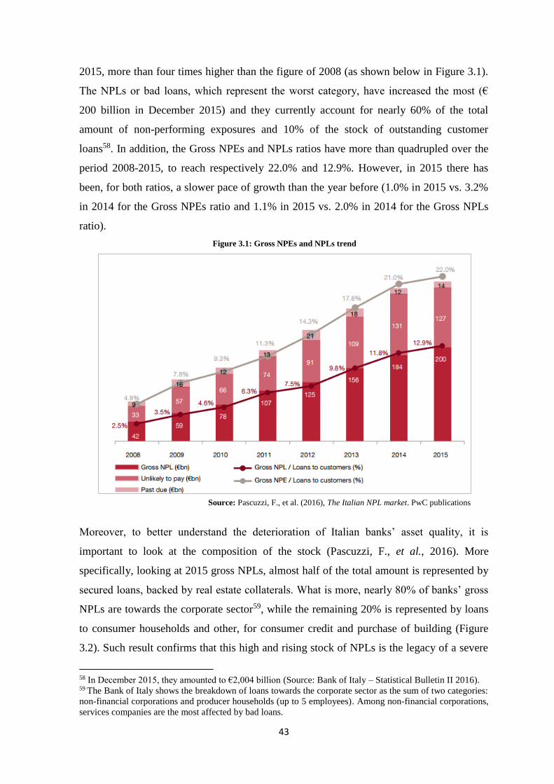
43
2015, more than four times higher than the figure of 2008 (as shown below in Figure 3.1).
The NPLs or bad loans, which represent the worst category, have increased the most (€
200 billion in December 2015) and they currently account for nearly 60% of the total
amount of non-performing exposures and 10% of the stock of outstanding customer
loans58. In addition, the Gross NPEs and NPLs ratios have more than quadrupled over the
period 2008-2015, to reach respectively 22.0% and 12.9%. However, in 2015 there has
been, for both ratios, a slower pace of growth than the year before (1.0% in 2015 vs. 3.2%
in 2014 for the Gross NPEs ratio and 1.1% in 2015 vs. 2.0% in 2014 for the Gross NPLs
ratio).
Moreover, to better understand the deterioration of Italian banks’ asset quality, it is
important to look at the composition of the stock (Pascuzzi, F., et al., 2016). More
specifically, looking at 2015 gross NPLs, almost half of the total amount is represented by
secured loans, backed by real estate collaterals. What is more, nearly 80% of banks’ gross
NPLs are towards the corporate sector59, while the remaining 20% is represented by loans
to consumer households and other, for consumer credit and purchase of building (Figure
3.2). Such result confirms that this high and rising stock of NPLs is the legacy of a severe
58 In December 2015, they amounted to €2,004 billion (Source: Bank of Italy – Statistical Bulletin II 2016). 59 The Bank of Italy shows the breakdown of loans towards the corporate sector as the sum of two categories:
non-financial corporations and producer households (up to 5 employees). Among non-financial corporations,
services companies are the most affected by bad loans.
Figure 3.1: Gross NPEs and NPLs trend
Source: Pascuzzi, F., et al. (2016), The Italian NPL market. PwC publications

44
and protracted recession that hit many Italian firms in 2008, but even more it underlines the
high level of companies’ dependence, especially the SMEs60, on bank funding.
Other two relevant issues for the Italian banking sector, as highlighted by Jassaud and
Kang in their IMF Working Paper61, are the low cash provisioning and the slow pace of
write-offs, which contribute to the NPLs accumulation and the depression of banks’
profitability and valuations. With regard to the first point, the average NPEs coverage ratio
for Italian banks has declined since the onset of the financial crisis, from 48% in 2007 to
45% in 2015, with a low of 37% in 2012. Despite the slight upward trend over the last
three years (driven by the pressures of the ECB’s Asset Quality Review exercise) and the
fact the current ratio is in line with the average of the main European banks (BoI,
Financial Stability Report, April 2016), such improvement differs between the five bank
categories62, with large and minor banks having lower-than-average coverage ratios
(respectively 43.4% and 40.8%). On the other hand, the slow pace of write-offs, which is
partly related to a general tendency of Italian banks to manage NPLs internally and write
them down instead of having them removed from the balance sheet, has essentially lead to
a situation in which new bad loans are not offset by adequate outflows (Figure 3.3).
60 This high dependence of small and medium sized companies can also be explained by looking at the
distribution of bad loans by amount, provided by the Bank of Italy in the Statistical Bulletin. In particular, it
is possible to see that, in terms of number of borrowers, nearly 75% of NPLs are related to loans the amount
of which is less than €75,000. 61 Jassaud, N., Kang, K. (2015), A strategy for developing a Market for nonperforming loans in Italy. IMF
Working Paper 62 The Bank of Italy divides banks into five size classes: “5 largest groups”, which comprises banks
belonging to the groups Unicredit, Intesa Sanpaolo, Banca Monte dei Paschi di Siena, UBI Banca and Banco
Popolare, “large banks”, which comprises banks with total assets greater than €21.5 billion, “small banks”,
which are those with total assets between €3.6 billion and €21.5 billion and “minor banks” which have total
assets below €3.6 billion.
Source: Pascuzzi, F., et al. (2016), The Italian NPL market. PwC publications
Figure 3.2: Gross NPLs breakdown

45
Indeed, there has been a gradually decline in the share of extinguished bad loans compared
to the stock of gross NPLs, reaching a low in 2014 (as shown in Figure 3.4).
Finally, it is important to stress how this asset quality deterioration and associated
provisioning have depressed banks’ valuations and earnings capacity. Indeed, even though
the Italian banking system is profitable overall, there is a significant heterogeneity across
banks (Jobst and Weber, 2016) and, especially the smaller ones, will likely continue to face
profitability challenges, even under favorable monetary conditions, due to the decrease in
net interest income and high operating cost63.
Furthermore, despite the better-than-expected results of EBA Stress Test, released last
July, Italian banks’ relative performance, with respect to Eurozone peers, continued to be
weak64 (e.g. the Texas ratio is still high at 110%). Looking also at trading multiples, it
results that Italian banks are trading at 0.47x 17E P/BV (Price to Book Value) vs. a
Eurozone average of 0.67x, implying a 30% discount, and that their 17E RoTE (Return on
Tangible Equity) equals 6.1%, which is 22% lower than the Eurozone average.
63 The highest among the ten largest economies in Western Europe, according to a study of “CGIA
Associazione Aritigiani Piccole Imprese Mestre”. More specifically, in 2014, 1.8% of Italian banks’ assets
has been spent as operating expenses (Jobst and Weber, 2016). 64 Credit Suisse Equity Research (2 September 2016). The cost of a potential NPLs deconsolidation.
Source: Cerved (2016), L’evoluzione dei crediti deteriorati in Italia e l’impatto delle riforme
Note: new bad loans are in green, while extinguished bad loans in blue (€bn on the y-axis)
Figure 3.3: New vs. extinguished NPLs
Figure 3.4: Extinguished NPLs as a % of Gross NPLs

46
3.2 A MARKET FOR NPLs IN ITALY
The problem of high and rising NPLs in Italy has been of great concern for a long time:
many academics and researchers have addressed this topic in their papers65, discussing the
barriers to NPL resolution and potential strategies to support economic recovery.
Concurrently, political authorities have tried to study and implement targeted actions to
reduce the stock of NPLs and trigger new lending.
All of that notwithstanding, today still persists the problem of a poorly developed
secondary market for NPLs that could sustain corporate and financial restructuring. Indeed,
alongside the high stock of NPLs, sales transactions are still limited; only for small
amounts in 2012-2014 (€17 billion of non-performing exposures, of which about €11
billion of bad loans), which however increased, in 2015, to approximately €19 billion (of
which about €9 billion of bad loans). This strong activity in the last year was in large part
due to the fact that Italian banks (especially Unicredit, MPS and Banco Popolare) have
started to prepare and implement deleveraging plans, having defined which assets to hold,
restructure, or sell66. In the first quarter of 2016, 8 new transactions of about €5 billion
have been registered (PwC predicts at least €30 billion GBV transactions for 2016).
Looking below at the breakdown of transaction volumes (Figure 3.5), we can see that the
majority of them are represented by disposals of consumer and retail unsecured credits.
65 See, for example, Jassaud, N., Kang, K. (2015), A strategy for developing a Market for nonperforming
loans in Italy. IMF Working Paper; Garrido, J., et al., (2016). Cleaning-up Bank Balance Sheets; Economic,
Legal, and Supervisory Measures for Italy (No. 16/135). International Monetary Fund; Jobst, A., Weber, A.
(2016), Profitability and Balance Sheet Repair of Italian Banks (No. 16/175). International Monetary Fund 66 KPMG, European Debt Sales Report: 2016 edition (February 2016).
Source: Pascuzzi, F., et al. (2016), The Italian NPL market. PwC publications
Figure 3.5: NPEs transactions in the Italian market (€ bn)

47
The main reason is that the unsecured retail loans prove to be the more easily transferable
asset class, compared with other clusters, due to the limited capital loss generated on their
disposal. However, more transactions involving secured portfolios (commercial and
residential real estate loans) are expected to occur in 2016, thanks to the long awaited
recovery in the Italian real estate market. Expectations remain instead low for SMEs and
corporate loan transactions.
Considering then the market participants, the sell-side is represented by a large number of
Italian and foreign-owned banks, which are under pressure from the ECB to clean up their
balance sheet, whereas, the buy-side is still characterized by a low number of large scale
international investors (Fortress, Cerberus, Apollo etc.) and specialized players with a
strong partnership with local servicers (Credito Fondiario, Anacap, Banca IFIS etc.).
Certainly, looking at other countries such as Japan and the United States, where markets
for NPLs are more liquid and have generally existed for longer, it is clear that the whole
European market for distressed debts is still small and at an early stage, especially in terms
of transactions volumes over the outstanding stock of NPLs. The market is mainly
characterized by outright sales and JVs between banks, investors and servicers, and it
primarily focuses on commercial real estate and consumer loans (Aiyar, S., et al., 2015).
However, as well as in Italy, also in Europe 2015 has been a record year, with transactions
amounting to €141 billion67, more than 10 times higher than in 2010 (Figure 3.6).
Most of the activity has taken place in the United Kingdom and Ireland, respectively with
approximately €40 billion and €25 billion of successfully sold loan portfolios. This result is
mostly due to the large transactions undertaken by their respective systemic bad banks, the
UK Asset Resolution Limited (UKAR) and the National Asset Management Agency
67 KPMG, European Debt Sales Report: 2016 edition (February 2016).
Source: Capitalising on the acceleration in bank restructuring, PwC publications (2016)
Figure 3.6: NPEs transactions in Europe

48
(NAMA)68. In addition, it is worth noting that both the UK and Ireland are already shifting
their deleveraging strategies from larger commercial real estate to residential mortgage and
SMEs NPLs.
Why, then, does Italy have lagged behind other EU countries and, only now, it is showing
signs of picking up?
3.2.1 MAIN IMPEDIMENTS
Yet, in the past (1997-2005), it has existed an Italian market for NPLs, which was even
considered by many one of the largest reference markets outside the United States and
Japan69. More specifically, the rise of the market started with the enactment of the Italian
securitization Law 130/1999, which allowed many Italian banks to dispose of their NPLs.
The main reason for this was that the Law provided a specific fiscal incentive to lessen the
transfer cost: banks were, indeed, allowed to recognize NPL-related losses over a period of
five years after the securitization. Between 1999 and 2005, more than €30 billion of bad
loans were securitized.
However, with the expiration of the tax and accounting-related benefits in May 2001
(Fabozzi and Choudhry, 2004) and the subsequent downfall of the securitization process
after the global financial crisis, the Italian NPL market has significantly slowed down.
But what were the barriers that have prevented so far the renaissance of this market?
According to Jassaud and Kang (2015), the limited NPL market activity in Italy has to be
attributed to both supply and demand factors. In particular, on the supply side, banks are
less incentivized to dispose of their NPLs due to:
Low level of provisioning: in such situation, selling NPLs would imply discounts on
the loan book value, as well as it would mean recognizing losses which would
immediately undermine the bank’s capital buffer. When provisioning is too low,
banks are also incentivized to hold on their NPL portfolios in order to preserve their
coverage ratios;
68 UKAR was established in 2010 and is wholly owned by the HM Treasury UK, while Ireland’s NAMA was
established in 2009 by the Government of Ireland (KPMG, European Debt Sales Report: 2016 edition,
February 2016). 69 Fabozzi, F. J., Choudhry, M. (2004), The handbook of European structured financial products (Vol. 131).
John Wiley & Sons

49
Limited capital buffers: the low level of NPLs sales can be explained by the
inadequate level of capital (e.g. a Texas ratio above 100%) set aside by banks to
absorb potential losses;
Heavy reliance on collateral coverage: as stated in the Financial Stability Report of
April 2016, half of Italian gross non-performing loans are secured by collateral
(67% including personal guarantees). However, even though collaterals represent a
protection against the possibility of losses, they can incentivize banks to internally
manage their bad loans and collect the value only at the end of the foreclosure. In
short, Italian banks have what Jassaud and Kang (2015) call “a zero-cost call
option” to delay the loan value recovery;
Close bank-borrower relationship: traditionally, Italian banks, especially the small
cooperative banks (BCCs), have always granted loans based on close, long-
standing relationships with borrowers. In this context, massive sales of non-
performing loans could compromise the reputation of the bank. It is also important
to highlight that a close bank-borrower relationship, while it can help banks to
better overcome information asymmetry problems, on the other hand, it can result
in relaxed lending standards and, thus in higher NPLs;
Servicing costs: there may be an incentive for banks to internally manage NPLs due
to high servicing costs or because of servicers do not necessarily provide all-
inclusive services (they may be specialized only in certain asset classes or
geographical areas);
Unfavorable tax regime for provisioning and write-offs: until 2013, Italian banks
were not allowed to deduct write-offs in the absence of a court declaration of
insolvency and only loan loss provisions up to 0.3% of total outstanding loans were
directly deductible from IRES, the corporate income tax (while the rest over a
period of 18 years). In 2013, the Law has been amended (but still remains more
restrictive than EU standards) by reducing the deductibility period from 18 years to
5 years, removing the 0.3% threshold and extending its provisions to the regional
tax on production (IRAP)70;
Favorable accounting rules for holding NPLs: first, the lack of a specific rule about
when to write-off uncollectible loans, under IAS 39, has led Italian banks to apply
the derecognition rule (i.e. wait until all possibilities for the collection are
70 Natixis (2016), Will Italian banks manage to get rid of their bad debts? Cross-Expertise Research

50
exhausted and contractual rights on cash flows are given up, rather than follow a
prudential timely write-off)71. Second, since IAS 39 allow interest on impaired
loans (not in the case of bad loans) to be accrued, banks are encouraged to retain
NPLs, given the subsequent positive impact on their income and provisioning ratio.
And third, incentives to restructure NPLs are weakened directly by the backward-
looking approach of IAS 39 to loan provisioning, which permits recognition of
credit losses only when incurred, based on an “objective evidence” (Gaston, E.,
Song, M. I., 2014). This approach, which is expected to be replaced with an
expected loss based model, when IFRS 9 will become effective in 2018, may result
in insufficient provisions;
Priority claim of public creditors: the privileged role of public creditors (for
example tax authorities) within bankruptcy procedure may discourage banks from
restructuring NPLs.
On the other hand, factors limiting demand for distressed debts are the following72:
Information asymmetry between originating banks and investors: the slow disposal
of NPLs in Italy is largely due to the lack of complete and well-organized banks’
databases, public asset and real estate transaction registers. In the majority of cases,
historical data are not accurate, still in a printed format and not readily obtainable;
therefore, investors are not able to properly assess NPLs portfolios in a timely
manner;
Length and inefficiency of foreclosure and insolvency procedures: NPLs
restructuring is also hampered by the slow and inefficient Italian judicial system.
Legal uncertainties around the recovery times73 of unpaid debts have frozen
investors’ demand so far, due to higher legal costs of debt restructuring and lower
expected recovery rates;
Market conditions: investors are still concerned about the medium-term prospects
for Italian economy and, even more, about the stability of the country’s banking
system;
71 The derecognition rule was actually designed for events such as the sale or transfer of financial instruments
or when the financial rights to cash flows from a financial instrument expire (Gaston, E., Song, M. I., 2014). 72 Jassaud, N., Kang, K. (2015), A strategy for developing a Market for nonperforming loans in Italy. IMF
Working Paper; Quaestio Capital Management SGR (2016), Atlante Fund Presentation. 73 According to a market study conducted by Cerved Credit Management, the average duration of bad debts
has been estimated in 7.3 years (as a weighted average of lengths and volume of insolvencies in the
categories: “insolvency proceedings”, “foreclosure on real estate” and “seizure of 20% of salary”).

51
Limited investor base: in Italy the audience of institutional investors (private equity
funds, pension funds and insurance companies) is still limited, as well as the
portion of capital invested.
3.2.2 POTENTIAL BENEFITS
Considering that today the problem of NPLs is a “systemic” problem that impacts the
economy as a whole and prevents the necessary recovery, the presence of an active and
liquid secondary market for distressed loans (and collaterals) would encourage banks to
dispose of their NPL portfolios and it would release enough resources to support credit
growth (Jassaud and Kang, 2015).
In addition, being a more-cost effective alternative to internal management and court
restructurings, a market for NPLs would contribute to reducing the burden on banks,
especially the smaller ones (because of a lack of expertise and economies of scale or
scope), and increasing loan recovery values, with the help of outside financing and
expertise (Aiyar, S., et al., 2015). In this respect, Italian banks could both sell directly their
NPLs on the market or leverage key skills and competencies of outside investors, through
specifically-created special purpose vehicles74. It would also improve banks’ risk
management practices, as well as support the recovery of the corporate sector by providing
additional non-bank sources of funding, in the short-term, and promoting a general
reallocation of resources over time.
Finally, a market for NPLs could trigger a virtuous circle in which the restructuring
process would reestablish confidence between borrowers and creditors, lead to higher
banks’ profitability and unlock new lending to firms and households.
3.3 THE PROBLEM: A WIDE BID-ASK SPREAD
The true problem with the inefficiency of the NPLs market in Italy, which is eventually the
result of all the above-mentioned impediments, is the wide difference between the price at
74 An important example, in this sense, is represented by the agreement reached between Unicredit, Intesa
Sanpaolo and KKR Credit in June 2015. In particular, the two Italian banks will transfer selected corporate
loan portfolios into a vehicle managed by a fully privately funded platform launched by KKR Credit. The
platform aims to provide long-term capital and operational expertise to support Italian banks in managing
assets. [https://www.unicreditgroup.eu/en/press-media/press-releases/2015/intesa-sanpaolo--unicredit--kkr-
credit-sottoscrivono-accordo-a-s.html]

52
which banks would be willing to sell their NPLs and the price at which investors are
willing to buy; the so-called “bid-ask spread”. Such difference is always a constant feature
of transactions and it generally differs according to the underlying asset (for example, it
can range from 2.5%-5% for corporate bonds amounting up to €200 million, to 10%-20%
for non-liquid shares)75.
However, why does in Italy the average differential between NPLs’ net book value (NBV)
and the market price is so wide76, as to prevent the development of a secondary market? To
be precise, as of today, the disagreement between supply and demand of NPLs is around
20%77. Indeed, on the supply side, the ideal sale price for a bank is the difference between
the nominal value and the current level of loan loss provisions: according to the last
Financial Stability Report, as of December 2015 the average coverage ratio for bad debts
was 59%; therefore, today banks are willing to sell their NPLs at approximately 41% of the
nominal amount. On the demand side, instead, investors (specialized operators, hedge
funds, etc.) are mainly concerned about the portion of the nominal amount that can be
recovered after the disposal. Generally, there are no indicative market prices, since the
market is still underdeveloped and prices can vary substantially depending on the type,
collateral and amount of the coverage78.
75 Quaestio Capital Management SGR (2016), Atlante Fund Presentation 76 To be precise, the wide bid-offer price gap mainly relates to secured NPLs, as banks and investors apply
different valuation criteria. The high coverage of unsecured NPLs, instead, helps the closing of many deals.
(Credit Suisse Equity Research, Italian Banks, 20/07/2016). 77 Natixis (2016), Will Italian banks manage to get rid of their bad debts? Cross-Expertise Research 78 Ciavoliello, L.G., et al. (2016), What’s the value of NPLs? Notes on Financial Stability and Supervision
No. 3
Source: Natixis (2016), Will Italian banks manage to get rid of their bad debts?
Figure 3.7: Price gap between supply and demand for NPLs

53
However, it is argued that the majority of investors are prepared to pay, on average, up to
20%, thus leading to the above price gap of 21-23% (Figure 3.7) and the subsequent
mismatch between demand and supply.
Among the factors that determine this wide pricing gap (also referred to as a “haircut” on
the net book value) there are, as previously seen, the quality of data and documentation
available to investors, the tax rules for provisioning, the costs and efficiency of the
servicing segment, the market conditions, the rate and time of collateral decay, and so on.
Above all, however, it is possible to say that the pricing gap is a function of (i) the NPL
discount rate (or the investor’s required return) and (ii) the expected recovery time of the
distressed assets’ residual value. This gap can widely differ from country to country (and
even within the same country) depending on the effectiveness of the legal and judicial
systems, the efficiency of banks’ internal procedures and the return expectations of
distressed debt investors.
Obviously, the longer the recovery time, the higher will be the return required by investors
and, subsequently, the pricing gap, thus discouraging banks to dispose of their NPLs79. In
this respect, it should not seem strange that Italy has such a wide pricing gap: just thinking
about the duration of the foreclosure procedures (as shown above in Figure 3.8), evidence
shows that Italy is the worst country in the Eurozone, with an average recovery time of 56
months (~5 years) against the 24 months in Greece and Portugal and the only 5 months in
the Netherlands (Garrido, J., et al., 2016).
79 The market price is heavily affected by the average duration of legal procedures; that’s why similar
transactions in other countries cannot be used as comparable when setting the price.
Source: Garrido, J., et al., (2016), Cleaning-up Bank Balance Sheets; Economic,
Legal, and Supervisory Measures for Italy (No. 16/135), IMF
Figure 3.8: Average length of foreclosure procedures by country

54
Moreover, recovery times of cash flows not only affect the valuation of NPLs (to such an
extent that it is estimated an increase of 10 percentage points in the market price with a
two-year reduction in recovery times80), but also their equilibrium value. In particular, it
has been shown that two banking systems that differ only for the recovery time (e.g. 2
years and 5 years) but have the same loan growth rate (e.g. 5%) and the same rate of new
NPLs (e.g. 2%), would have in equilibrium a ratio of bad loans over total loans
respectively equal to 3.5% and 7.4% (Ciavoliello, L.G., et al., 2016).
In addition to these cross-country variations, however, one of the main reasons explaining
the substantial bid-ask spread lie in the different valuation criteria used by banks and
investors in determining the NPL value and, especially, those pertaining to the discount
rate to be applied to expected cash flows and the treatment of direct and indirect costs.
3.3.1 BANKS VS. INVESTORS’ VALUATION PERSPECTIVE
Different criteria for different valuation perspectives: while the primary objective for banks
is to purse low-risk work-out strategies in order to minimize losses, investors are willing to
speculate as much as needed to increase returns.
On one hand, Italian banks, as well as most of the European banks, recognize their loans
on the basis of the applicable international accounting principles (IAS-IFRS). In particular,
as already explained in the previous chapter, IAS 39 requires banks to measure their loans
at amortized cost using the effective interest method. Thus, the loan gross book value
(GBV) is given by the sum of the future expected cash flows, over the life of the loan,
discounted at the original effective interest rate. This rate currently ranges from 4% to 5%,
which necessarily results in a higher selling price.
The same mechanism is applied in case of non-performing loans. More specifically, the
bank should evaluate (i) the recoverable amount, which is also related to the collateral
value, (ii) the recovery rate (i.es. one minus the Loss-Given-Default) and (iii) the recovery
time (which is different from that contractually agreed). The NPL’s net book value (NBV)
is then computed by discounting the new lower expected cash flows, adjusting for the new
higher recovery time (in order to account for the duration of the collateral sale procedures).
The difference between NPL’s GBV and NBV is represented by the loan loss provision to
be recognized in the profit and loss account (P&L) for the period.
80 Based on the strict assumption of an IRR of 15-25% (Ciavoliello, L.G., et al., 2016)

55
Over time, the difference will be given by the sum of all recorded write-downs and write-
backs (in the case in which the debtor becomes solvent again).
In addition, banks are required, consistently with the international accounting principles, to
consider the direct costs of managing NPLs (such as the costs of collecting and selling the
guarantee) directly in the computation of expected cash flows, whereas the indirect costs
(such as personnel expenses and servicing fees) should be recognized in the P&L of the
period in which they are incurred (Ciavoliello, L.G., et al., 2016).
On the other hand, instead, distressed debt investors generally reach lower NPL valuations,
due to:
Different estimates of the loan’s future expected cash flows, because of information
asymmetries in the market which force them to apply haircuts to the expected
recoverable amounts provided by banks;
Even assuming that banks and investors’ estimates of expected cash flows are the
same, the latter apply a different discount rate since they require a higher return (as
of today, the IRR ranges from 10% to 25%) on investment, which includes a risk
premium, generally greater the higher the dispersion of potential recoveries around
the average value. In particular, investors’ IRR is much higher because (i) they
generally have a lower financial leverage than banks, (ii) they tend to be more risk-
averse and (iii) they have to account for fund managers’ fees. Then, potential
information asymmetries can also be factored in a higher discount rate81;
Investors immediately deduct all costs of managing NPLs, both direct and indirect,
from the net book value;
Potential acquirers can also attribute zero enterprise value (EV) to corporate NPLs
or apply haircuts in case of non-listed companies or audit reports not released by
international accountants82.
Figure 3.9 shows the different valuation perspective of banks and investors and how they
come up to a different NPV.
81 Credit Suisse Equity Research, Italian Banks (20/07/2016). [http://www.sipotra.it/wp-
content/uploads/2016/07/Credit-Swiss_Italian-banks-Report_20.07.16.pdf] 82 Sheehan, J.M., (2011), Optimising Distressed Loan Books: Practical Solutions for Dealing with Non-
performing Loans. Harriman House

56
In particular, starting from the EV that secure each loan, investors adjust for the expected
recovery rate, deduct the collection costs and then discount back at a rate between 15% and
25%83.
Jobst and Weber (2016) have proposed a calculation approach for this pricing gap between
book values and market prices, which immediately reflects one of the main inherent causes
for it, that is, the use of an incurred loss-based model by banks, on one hand, and of an
expected loss-based model by investors, on the other hand. More specifically, it is
computed (in percent of each unit of NPLs) as the difference between an implied coverage
ratio and the actual coverage ratio. Considering a loan with a fully provisioned unsecured
portion of 15% (of the principal value) and the remaining 85% secured by collateral, the
implied coverage ratio is estimated as follows:
[0.15 + (1 −((0.85 ∗ (1 − 𝑟𝑐) ∗ 𝑒−𝑟𝑡 ∗ (1 − 𝐿)) − 𝑀)
0.85)]
Where 𝐿 represents the legal/servicing fees (in percent), 𝑀 the management costs (in
percent), 𝑟 is the required rate of return by investors, 𝑟𝑐 is the collateral rate of decay and 𝑡
the expected recovery time of collateral.
83 Assuming high discount rates and low recovery rates, we can say that investors discount cash flows twice.
That’s why they come up to such a low NPL’s valuation (Sheehan, J.M., 2011).
Figure 3.9: Banks vs. Investors’ valuation perspective
Source: Sheehan, J.M., (2011), Optimising Distressed Loan Books: Practical Solutions for Dealing with
Non-performing Loans. Harriman House

57
3.4 CRITICAL ISSUES IN REDUCING THE GAP
Once raised the issue of this wide bid-ask spread, it is important to stress that there are not
so many viable solutions for a quick and efficient reduction.
In general, to reduce the gap one could envisage either a higher NPL coverage ratio or a
higher NPL market price84. In the first case, however, a coverage uplift would force banks
to recognize additional provisions and losses and, therefore, to recapitalize in order to both
absorb the additional losses and to comply with the Basel requirements (i.e. cover potential
capital shortfalls to the SREP85).
The second way, instead, could be achieved with a reduction either in the recovery time or
in investors’ return. However, only the former seems to be a more realistic solution, even if
it requires the necessary involvement of public authorities in the shortening of the
foreclosure times. This because investors are generally unwilling to reduce their IRR,
especially in the context of a market characterized by many forced sellers and a low
number of buyers. Therefore, it would be more likely that originating banks increase their
discount rate, consistently with the equity funding of NPLs. Nonetheless, even in this case,
additional impairments will be required.
Two ways that have been proposed to solve the problem were: (i) aligning the book value
of NPLs to the market price and (ii) create a systemic bad bank that allows Italian banks to
transfer NPLs at a government-subsidized price. However, it has been shown that both are
almost impossible to implement86.
3.4.1 ALIGNING THE BOOK VALUE TO THE MARKET PRICE
Aligning the book value of non-performing loans to the current market prices (which is
eventually the same as having a higher NPL coverage ratio), would mean to impair the net
value of bad loans by 50-55% and, therefore, to recognize additional losses (net of tax
deduction at 27.5%) of about €30-33 billion. Table 3.6 contains a sensitivity analysis of the
impact on the aggregate sector’s CET1 and the implied LGD on bad loans, with respect to
the haircut applied on NPL’s net value. Assuming this massive write-offs, Italian banks
84 Credit Suisse Equity Research, Italian Banks (20/07/2016). [http://www.sipotra.it/wp-
content/uploads/2016/07/Credit-Swiss_Italian-banks-Report_20.07.16.pdf] 85 Within the supervisory review and evaluation process (SREP), the European Banking Authority (EBA)
assesses whether banks’ capital resources are adequate and provides the capital requirement (CET1) that
banks have to meet on a consolidated basis. 86 Natixis (2016), Will Italian banks manage to get rid of their bad debts? Cross-Expertise Research

58
would eventually have an aggregate CET1 ratio between 9.6-9.9%, much lower than the
average 12.3% (11.5% for significant banks) at the end of 2015.
This solution does not seem to be realistic, for both financial stability and political reasons.
Indeed, on one hand, banks would not be willing to book massive capital losses at one
time, preferring instead a gradual recovery of their asset quality over time. Moreover, on
the other side, the government would be reluctant to the idea of re-imposing additional
losses to the Italian banking system, after the bail-in of about 12,000 subordinated
bondholders during the resolution of four small banks (Banca Marche, Banca Etruria,
Cassa Risparmio di Ferrara and CariChieti), in November 201587. This event has had
significant implications for the banking sector, among which, in particular, the increased
concern about Italian banks’ asset quality and the establishment of a dangerous benchmark
for future transactions.
3.4.2 THE IMPOSSIBILITY OF AN ITALIAN BAD BANK
The second solution is even more unlikely, since it would not comply with the current EU
State aid rules, updated in August 2013, which define the common conditions under which
87 The resolution of these four small banks (split into a new “good bank” and a “bad bank”) represented the
first bail-in in Italy and it has been characterized by a large mark-down imposed by the EU (non-performing
loans were indeed written down by 80%, from the original value of €8.5 billion).
Source: Natixis (2016), Will Italian banks manage to get rid of their bad debts?
Table 3.6: Impact of a haircut on NPL’s net value

59
the EU Member States can support financial institutions during crisis, with funding
guarantees, recapitalizations or asset relief. The main changes, aimed at improving the
level playing field between similar banks and at reducing the market fragmentation, have
concerned (i) the implementation of a sound restructuring plan, to return to long-term
viability, before asking for recapitalizations and (ii) the forced contribution, in case of
capital shortfalls, of bank owners, junior creditors and hybrid instruments holders, before
the use of public funding88.
Consequently, as of today, it is not possible to create a systemic bad bank such as those set
up in Ireland (NAMA) and in Spain (SAREB), respectively in 2009 and 2012. Indeed,
those public asset management companies, even though mainly financed by the private
sector, have had the possibility to issue NPL-backed securities with the government’s
guarantee, free of charge, and therefore, to trigger the development of a distressed debt
market. Instead, a similar sale of NPLs at “above market price” would imply, today, the
“burden-sharing principle”, as stated before.
In order to be compliant with EU State aid rules, a possible structure for a public AMC
should have the following characteristics (Aiyar, S., et al., 2015):
Transfer at market price: NPLs should be transferred at market prices or, in case of
market illiquidity, at a price agreed with the EU Directorate-General for
Competition;
Semiprivate ownership: public involvement should be limited to a minority stake so
that the bad bank’s liabilities would be only contingent liabilities for the state;
Governance: a clear mandate, to maximize assets’ recovery value in a
predetermined period of time, should be assigned in order to avoid moral hazard
behaviors;
Voluntary participation by banks: banks should still be allowed to internally work
out their NPLs or use private bad banks;
Strengthening NPLs recovery value: temporary powers, such as fast-track
restructuring solutions, should be granted to overcome specific structural problems.
88 “State aid: Commission adapts crisis rules for banks” [http://europa.eu/rapid/press-release_IP-13-
672_it.htm]. According to Art. 107(3b) of TFEU (Treaty on the Functioning of the European Union), it
constitutes an exception the State aid “to promote the execution of an important project of common European
interest or to remedy a serious disturbance in the economy of a Member State”.

60
CHAPTER 4
GOVERNMENT STRATEGIES AND
POTENTIAL IMPACTS
4.1 A THREE-PRONGED STRATEGY
Since 2014, when the EBA released the AQR and stress test results and raised the need for
further structural reforms, the Italian Government has started to address the problem of
high NPLs, implementing a number of actions and reforms.
In particular, it has developed a three-pronged strategy consisting of (i) a package of
structural reforms aimed at improving the fiscal and corporate insolvency regimes, (ii) a
state guarantee scheme, also known as “GACS” (Garanzia sulla Cartolarizzazione delle
Sofferenze), to facilitate the NPL securitization and (iii) the launch of “Atlante”, a private
fund whose purpose is to act as a buyer of last resort for those banks that face market
difficulties.
These initiatives, put in place since the beginning of summer 201589, seem to have already
produced benefits in terms of increased market liquidity and greater investors’ interest and
commitment towards the Italian NPLs market, which still remains one of the largest
potential markets for distressed debts with its stock of non-performing exposures of about
€341 billion. As previously mentioned, indeed, volumes of transactions have more than
doubled in 2015, compared to the previous year (€19 billion vs. €8 billion), and at least
€30 billion are expected to be sold in 2016 (Pascuzzi, F., et al., 2016). Moreover, investor
base is growing, both with the strengthening of incumbents and the entrance of new
89 It is worth noting that, in parallel with this three-pronged strategy, the Italian Government has started the
implementation of several legal and regulatory reforms aimed at facilitating the consolidation of the banking
system. In particular, in March 2015 the Senate approved the reform of cooperative banks (banche popolari),
which forced those with assets above €8 billion to become joint stock companies (or alternatively to reduce
their assets below the threshold or liquidate). In February 2016, it has been approved the reform of mutual
banks (banche di credito cooperativo) with a net equity below €200 million. It provides for the establishment
of a parent company with a minimum equity of €1 billion, the majority of which should be held by the BCCs
(which in turn can opt for the transformation into joint stock company) (Pascuzzi, F., et al., 2016).

61
players (such as pension funds, social security and insurance companies which are looking
for yield due to the current low-interest rate environment), and more structured deals are
started to replace single asset transactions.
In short, it is clear and widely accepted that government reforms are going in the right
direction to encourage the banks’ deleveraging and de-risking process and to help kick-
start the Italian market for NPL sales and securitization. However, major concerns still
remain about the extent to which this three-pronged strategy will be truly effective;
something that could be judged only in the coming years.
4.1.1 STRUCTURAL MEASURES
The package of structural measures adopted by the Italian Government has involved both
legal and fiscal aspects, with the specific purpose of stimulating, respectively, the demand
and supply of NPLs, and ultimately reducing the price gap in the secondary market90. More
specifically, on one hand, reforms tried to stimulate investors’ demand by facilitating the
recovery of bad loans and collateral, while, on the other hand, they tried to incentivize
banks to write-off their NPLs, through a more favorable taxation of provisioning.
Foreclosure and Insolvency Law Reform
In June 2015, the Italian Government approved Law No. 132/2015 (then enacted by the
Parliament in August), amending the Bankruptcy Law and the Civil Procedure Code in
force, with the purpose of improving the available restructuring tools (i.e. out-of-court
procedures and the so-called “concordato preventivo”91) and speeding up insolvency
procedures. The major highlights of the reform can be summarized as follows92:
“Holdout problem” overcoming: the Law has introduced a new mechanism to
address the common delays caused by opportunistic behaviors of the minority of
creditors, for those companies willing to conclude out-of-court restructurings and
with a financial debt amounting to at least half of overall liabilities (however, they
should be supported by 75% in value of the other creditors);
90 Natixis (2016), Will Italian banks manage to get rid of their bad debts? Cross-Expertise Research 91 It is a specific restructuring procedure, carried out under the court supervision, in which the debtor’s
restructuring plan should be approved by the majority of creditors and then confirmed by the court. 92 Marcucci, M., et al. (2015), The changes of the Italian insolvency and foreclosure regulation adopted in
2015. Notes on Financial Stability and Supervision No. 2

62
Competing restructuring plans and bids: creditors of companies in “concordato
preventivo” can submit a competitive plan with the one of the debtor (provided that
they represent at least 10% of the financial debt and debtor’s proposal does not
ensure the reimbursement of at least 40% of unsecured debts), as well as alternative
competing bids for assets subject to disposal are accepted from any interested party;
New requirements for insolvency administrators: in order to promote higher
transparency in the appointment of administrators and liquidators, it has been
introduced an online database including all relevant data about these professionals
and open to public inspection. In addition, administrators are now obliged to
provide the liquidation plan within 180 days from the date of declaration and finish
the process within two years (otherwise, they can be removed);
New best practices for the sale of collateral: the reform tried to improve the
efficiency in the foreclosure of collateral, by reducing the time-limits of certain
procedures and the possibility to have multiple auctions, allowing the judge to call
upon professional experts and successful tenderers to provide deferred payments.
Then, it mandates the Ministry of Justice to establish a national online database
containing information on all foreclosed assets’ sales and insolvency fillings.
The above-mentioned provisions have then been supplemented by Law Decree No.
59/2016 (“Decreto Sofferenze”), which introduced additional urgent legal and regulatory
measures, aimed at shortening the recovery times and aligning them to European standards.
Among others, the most remarkable ones are93:
“Pegno mobiliare non possessorio”: in line with the “floating charge” existing in
other jurisdictions, banks can now extend their pledge rights also on instrumental
movable assets, such as machinery or inventories, in addition to real estate
collateral. However, the businesses have now the possibility to transform, exploit
and/or dispose of the assets encumbered by pledge (while previously the property
was lost). This security interest must be entered in a specific online register held by
the Italian tax authority;
“Patto Marciano”: a contract by which creditor and debtor agree so that, in case of
default (i.e. when default is continuing for more than six month after the third
93 New Italian measures aimed at supporting businesses and accelerating credit recovery procedures - Law
Decree 59/2016 dated 3 May 2016. [http://knowledge.freshfields.com/en/Global/r/1468/new_italian_
measures_aimed_at_supporting_businesses_and]

63
monthly instalment is due), the real estate collateral (with the exception of the
entrepreneur’s residential property) can be automatically repossessed by the bank
or a designated real estate affiliate. In the case in which the appraisal value of the
asset is greater than outstanding debt and costs, the creditor shall pay the difference
to the debtor;
Compulsory expropriation: the Decree introduced new rules on credit recovery
procedures, among which the possibility to hold creditors’ meetings and hearings
using electronic tools, the provisional execution of an injunction order for the
portion of the claim not challenged by the debtor and the provision that no
oppositions are allowed if the disposal process has already started.
Taxation of Provisioning Reform
The Law No. 132/2015 has also introduced important amendments to the taxation of banks
provisioning, in order to facilitate the tax deductibility on loan losses and impairments. As
already mentioned in the previous chapter, Italian taxation has always been more
restrictive than European standards (until 2013, indeed, banks were only allowed to
directly deduct less than 0.3% of the total debt from IRES, while the rest over 18 years94).
However, with this reform, provisions for loans write-offs, write-downs and disposals may
be deducted from IRES and IRAP in the year in which they incurred. To be precise, the
Italian Government has introduced a transition period of ten years, starting from December
2014, according to which:
Until 2025, banks will be allowed to deduct only the 75% of write-offs and write-
downs’ provisions and related losses, in the year they are recognized, while the
remaining 25% and any losses not deducted as of December, 31st 2014 will be
spread over the 10-year period, according to a specific percentage (i.e. 5% in 2016,
8% in 2017, 10% in 2018, 12% from 2019 to 2024 and 5% in 2025). Losses on
disposals will always be 100% deductible in the year in which they incurred;
From 2026 onwards, instead, all provisions and losses will be deductible in the year
in which they are recognized.
Both reforms are expected to make a positive contribution to addressing the problem of
NPLs in Italy. In particular, the reform of insolvency and foreclosure regulation is
94 Natixis (2016), Will Italian banks manage to get rid of their bad debts? Cross-Expertise Research

64
expected to shorten the timelines of procedures and, consequently, to reduce investors’
required return, in the short time, and the equilibrium value of banks NPL ratio, over the
long term (Marcucci, et al., 2015).
A preliminary assessment, conducted by the Bank of Italy, has indicated that the duration
of a bankruptcy process should be halved in a favorable scenario (between -18% and -33%
in a worst-case scenario) and the length of real estate auctions should drop by a quarter.
Less optimistic is, instead, the report on NPL evolution by Cerved Credit Management95,
according to which the average recovery time of bad debts will drop from 7.3 to 6 years in
2020 (with an estimated -28% length of bankruptcies and -20% length of judicial
foreclosures). However, it also reports that, following the introduction of Law 132/2015,
there has been an increase in the number of bankruptcies completed (Figure 4.1), which
has passed from 6,383 over the period January-August 2015 (-4.7% YoY) to 7,234 from
August 2015 to March 2016 (+13.3% YoY). The reduction in the average length of
procedures (8 years in 2014 vs. 7.4 years in 2015) has actually started before its entry into
force, since it has been registered a contraction of 7.8% YoY from January to August 2015
and of 7.9% YoY from August 2015 to March 2016.
All this notwithstanding, there are still many question marks that reduce, in the current
perception of professionals, the actual “saving capacity” of the Government’s plan.
Amendments to the insolvency and foreclosure law are really enough to reduce debt
recovery times? The real question is about the whole judicial system which is clogged up
95 Cerved (2016), L’evoluzione dei crediti deteriorati in Italia e l’impatto delle riforme
Figure 4.1: Bankruptcies closed per month
Percentage, month over month of the previous year
Source: Cerved (2016), L’evoluzione dei crediti deteriorati in Italia e l’impatto
delle riforme

65
with cases and it is characterized by a lack of specialized judges and a high regional
heterogeneity in the quality of court enforcement (e.g. the average length of bankruptcy
procedures ranges from 5 years in Trentino-Alto Adige to 12 years in Sicily). Then, other
major limits of the reform concern the fact that it does not change the insolvency regime
for consumers and small enterprises and, especially, that it is not retroactive (not applicable
to existing claims, but only to new inflows of bad loans).
4.1.2 THE GACS (GARANZIA CARTOLARIZZAZIONE SOFFERENZE)
The second part of the government strategy is represented by the so-called GACS
(Garanzia sulla Cartolarizzazione delle Sofferenze), a fee-based guarantee scheme aimed
at facilitating the securitization of NPLs and, therefore, at increasing liquidity in the
secondary market. After the resolution of the four small banks in November 2015, the
government has started debates with the European Commission in order to find alternative
solutions to the creation of a systemic bad bank (given the restrictions imposed by the
BRRD96 and State Aid rules). In February 2016, they finally reached an agreement on this
GACS mechanism, which has then been introduced in April by the Law No. 49/2016.
96 The Bank Recovery and Resolution Directive (2014/59/EU) introduced a new framework for the recovery
and resolution of credit institutions and investment firms. According to the new rules, public intervention is
allowed only in circumstances of very extraordinary systemic stress and, in any case, after the bank’s
shareholders and creditors have borne losses equal to 8% of the bank’s liabilities.
[https://www.bancaditalia.it/media/approfondimenti/2015/gestione-crisi-
bancarie/index.html?com.dotmarketing.htmlpage.language=1]
Source: Natixis (2016), Will Italian banks manage to get rid of their bad debts?
Figure 4.2: NPL securitization under the GACS scheme

66
As shown in Figure 4.2, originating banks have now the possibility to clean up their
balance sheets by transferring bad loans, for a price not higher than their net book value, to
a private special purpose vehicle (SPV), which will in turn issue asset backed securities (in
at least two tranches, senior and junior/equity, and one or more optional mezzanine),
having NPLs as underlying assets.
The GACS scheme provides that only senior tranches (the least risky ones) shall be
covered by the state guarantee and, more specifically, only the contractual interest and
capital payment obligations of the senior noteholders. What is more, the government
guarantee can be granted only after the senior notes have received a rating, equal to or
higher than Investment Grade (BBB-, BBB, BBB+), from at least one rating agency, which
will evaluate, among others, cash flows, collateral value, loans credit quality, amount
invested in the junior tranches and the operating capacity of the appointed external
servicer97. In addition to the rating for the senior notes, the adoption of the state guarantee,
which however is not mandatory, requires that98:
The originating bank has to sell at least 50% plus one of the junior notes and,
anyhow, an amount of junior and mezzanine (if issued) notes such as to
deconsolidate and de-recognize the securitized assets;
The bank must appoint an external servicer responsible for the credit recovery. It
should not be affiliated with the selling bank in order to avoid any potential
conflicts of interest;
The cash flows deriving from the collection activity, net of all costs, shall pay in
priority interests on the senior notes, while the repayment of principal is
subordinated to the payment of interests on the mezzanine (if issued). The
junior/equity tranche shall be repaid only when all other tranches have been fully
redeemed. It may also be provided a deferred repayment of mezzanine tranches
under certain conditions or upon the achievement of certain performance targets;
The bank has to pay a price at market level in the form of an annual commission
proportional to the amount guaranteed, so that the issue of the state guarantee does
not constitute State aid. In particular, the price of the guarantee is calculated based
97 Deloitte, Italian non-performing loans. State guarantee and securitization scheme…Unlocking the NPL
log-jam? February 2016 [https://www2.deloitte.com/content/dam/Deloitte/uk/Documents/corporate-
finance/deloitte-uk-fa-italian-nonperforming-loans.pdf] 98 Natixis (2016), Will Italian banks manage to get rid of their bad debts? Cross-Expertise Research

67
on the average premium99 of a basket of single name Italian issuers CDS (whose
composition does not change over time and depends on the rating assigned to the
senior notes), with the same rating and duration of the guaranteed securities;
The price of the guarantee is increased in case the senior notes have not been fully
reimbursed by the end of the third or the fifth year from the grant of the guarantee.
This in order to incentive a quick recovery of the securitized debts.
Among other things, the GACS scheme is expected to incentivize banks to dispose of their
NPLs and to prompt the development of a market for NPL securitization, through both the
reduction in the funding costs of the SPV (by approximately 200bps, according to the MEF
guidance) and the increase in investor’s demand due to the higher credit worthiness of the
senior tranches. However, major concerns regard (i) the pricing of the guarantee, unlikely
to be accurate since the credit default swaps are generally hard to price, (ii) the amount of
time necessary to put it in place (for this reason, it is more plausible that it will be used for
large transactions), (iii) the type of credit enhancement that is needed to obtain the required
rating for the senior notes, (iv) the tranching process and the composition of the underlying
NPLs, given that the success of the scheme is determined by the placement of the junior
tranche100, and (v) the transfer price of bad loans to the SPV, since in the case of very low
prices, even though the risk of state aid would be limited, banks would be forced to
recognize additional losses and face potential capital shortfalls. In short, the GACS is
expected to have a positive impact, but only limited and clearly not sufficient to fill the gap
between investors’ market prices and book values (estimates of GACS contribution are
between 1-3 percentage points only, against a pricing gap around 15-20%).
Nevertheless, a positive result has been registered by Banca Popolare di Bari, the first bank
to take advantage of the GACS scheme in a €480 million (GBV) bad loan securitization,
comprising 63% secured loans and 37% unsecured loans to households and SMEs. The
vehicle has issued three tranches: a senior, with investment grade BBB (High)/Baa1 by
Moody's and DBRS of €126.5 million (3 years maturity and coupon equal to 6-month
Euribor plus 50bps), a mezzanine, with rating of B (High)/B2 by DBRS and Moody's of
€14 million (5-6 years maturity and coupon equal to 6-month Euribor plus 6%) and a
99 It is calculated over the six months preceding the issuance of the guarantee. 100 Indeed, it is worth noting that, if the junior tranche is not fully placed, it implies a capital absorption equal
to 100% of its nominal value, thus weighing on the bank’s solvency (the remaining portion of equity tranche
is deducted from CET1). Therefore, banks might be unable or unwilling to dispose of their NPLs at fire-sale
prices such as to gain sufficient demand for the junior tranche (Natixis, 2016).

68
junior, non-rated facility, amounting to €10 million (coupon not yet set but around 10-
15%). This transaction has been, not only the first of this kind in the Italian market, but it
has also reached a satisfactory level in terms of tranching and transfer price, which has
been set equal to 31% of the loans’ gross book value (~ €148 million)101. A value that is
definitely above the 20% obtained on average, by selling NPLs directly without
securitization, and that is in line with the announced 33% for the upcoming disposal of
Banca Monte dei Paschi’s entire bad loan portfolio (€27.7 billion gross at a sale price of
€9.2 billion). In short, the first use of the GACS has outperformed market expectations and
set a positive benchmark for what will be the world’s biggest NPL securitization.
However, the positive impact of the GACS mechanism is enhanced thanks also to the third
part of the government’s strategy, the launch of the Atlante fund.
4.1.3 THE ATLANTE FUND
The other important initiative, launched in April 2016, has been the Atlante fund, a closed-
end alternative investment fund participated by the main Italian banks (among which,
Intesa Sanpaolo and UniCredit subscribed a €1 billion stake each), banking foundations,
insurance companies, other institutional investors102 and the publicly-owned Cassa
Depositi e Prestiti (CDP), which contributed with €500 million. The fund has raised €4.25
billion (but with a potential leverage up to 110% of its capital) and has an investment time-
frame of five years, which can be extended for another three years, each year.
Atlante has been promoted by Quaestio Capital Management SGR, which represents the
fund’s asset management company, and supported by the Italian Government as an
alternative solution to the creation of a public bad bank. Indeed, the fund constitutes, using
the words of the Italian Minister of Finance Mr. Padoan, “an entirely private operation”,
completely backed by private resources so as to comply with the EU State aid
regulation103. According to Quaestio Capital Management’s presentation104, the ultimate
purpose of the fund is to “promote the creation and development of an efficient market of
distressed assets in Italy”, which is then translated into two primary functions:
101 “Pop Bari sells bad loans with state guarantee, sets stage for MPS”
[http://www.reuters.com/article/eurozone-italy-banks-badloans-idUSL8N1AT29P] 102 67 investors overall, with no one holding more than a 20% stake. 103 However, the ECB will carefully monitor the governance of the SGR and of the opinions of the Investors’
Committee (made up of nine members and elected by the Investors’ Meeting). 104 Quaestio Capital Management SGR (2016), Atlante Fund Presentation
[http://www.quaestiocapital.com/sites/default/files/Quaestio_Atlante_Presentation_29_4_2016EN.pdf]

69
Invest up to 70% in Italian banks facing capital requirements’ problems (i.e. a
lower CET1 ratio than the SREP threshold), acting therefore as a back-stop facility
for those future share capital increases that the market cannot secure by itself or
that can entail a risk of bail-in and consequent systemic implications. This is what
happened in the case of Banca Popolare di Vicenza and Veneto Banca, whose
recapitalizations have been funded by Atlante with €1.5 billion and €1.0 billion,
respectively;
Invest at least 30% in Italian banks’ non-performing loans, by acquiring the riskiest
tranches (junior and/or mezzanine, if issued) of NPLs securitizations, or through ad
hoc vehicles and tangible or intangible assets for NPLs transactions. This is aimed
at stimulating competition and investors’ demand (provided that senior tranches are
covered by the GACS, which is essential to allow the multiplier effect in the equity
tranches) and, therefore, at reducing the current wide bid-ask spread. Indeed,
Atlante will require an IRR from the junior tranches lower than that traditionally
demanded by specialized investors105 (but, in any case, it should be adequate with
the IRR of a bond having an average rating of single B), with the purpose of
pushing up other players’ bids.
As we can see from Figure 4.3 above, the launch of Atlante has been positively welcomed
by the markets: from the presentation of the project on April 11th to April 26th, Italian
banks’ share prices rose by 20% on average, while their CDS spreads drop by 50 basis
points. This immediate re-rating of banks’ share prices has proved that Atlante represents
an important complement to the other government initiatives, implemented with the
purpose of sustaining the weak Italian banking system. In particular, the ultimate
105 Atlante fund’s objective is to generate a return of approximately 6% per annum, while investors’ return is
on average equal to 15%.
Source: Bank of Italy, Financial Stability Report No. 1, April 2016
Figure 4.3: Market reaction to the launch of Atlante fund
Share prices (Euro Stoxx Banks and FTSE Italy Banks) and CDS spread (basis points)

70
underlying mechanism, which the fund intends to exploit in order to support the market
prices of shares and NPLs, is that of expectations. Indeed, if the market knows that there is
someone willing to buy at a certain price, everyone (sellers and buyers) will expect that the
price cannot go below that level and will act accordingly, so the price actually stabilizes at
that level. In principle, “the buyer of last resort” would not even need to intervene
spending its resources: something similar to what happened with the famous “whatever it
takes” of the ECB President Mario Draghi.
But, for how long the fund will be able to condition market expectations? Indeed, while on
one hand the Atlante fund has contributed to inject fresh capital, avoiding the bail-in and
resolution of two troubled banks, on the other hand, many doubts still remain about its
credibility and its effective role in solving the problem of NPLs in Italy. In this respect, the
major market concerns regard: (i) the fund’s limited size (equity resources)106, which has
been drastically reduced after the recapitalizations of Banca Popolare di Vicenza and
Veneto Banca, (ii) the presence of few specialized investors with high bargaining power,
which potentially complicates the fund’s task of boosting competition in the market, (iii)
the lack of impartiality with respect to the market that it wants to stabilize, since the fund
mostly consists of market participants and (iv) the potential risk of a domino effect in the
long term, due to the increased exposure of stronger banks (those investing in the Atlante
fund) to weaker institutions.
In short, Atlante seems to be only a “second-best choice”, useful to address the most urgent
problems surrounding the Italian banking system (last but not least, the upcoming mega-
rescue plan of Banca Monte dei Paschi di Siena), but not conclusive. Moreover, Quaestio
Capital Management’s presentation itself states that the success of the project will heavily
rely on the following external factors:
The actual changes prompted by the insolvency and foreclosure law reforms, since
a sound legal system is a necessary condition of any financial system;
The ability of banks to return to high profitability levels, since the disposal of NPLs
depends on their capacity to absorb old losses;
106 For this reason, on 8 August 2016 a second closed-end fund “Atlante II” has been set up with an initial
size of ~€2 billion (the final target, to be achieved in a year, is €3.5 billion) and a specific focus on NPLs (or
instruments linked to NPL deals, such as warrants). In particular, the Fund will buy the €1.6 billion
mezzanine tranche of the securitized NPLs of Banca Monte dei Paschi di Siena.
[http://www.quaestiocapital.com/sites/default/files/Comunicato%20Stampa%20Quaestio%20Atlante%20II%
2008.08.16%20ENG.pdf]

71
The trends in the Italian economy and the real estate market over the next years,
since the stock of bad loans also depends on the rate at which credit quality
deteriorates, from performing to impaired, and from impaired to bad loans.
4.2 POTENTIAL CONSEQUENCES FOR THE LISTED BANKS
So far it has been presented the problem of the lack of a secondary market for NPLs in
Italy, as well as the Italian government response through the above-mentioned threefold
strategy. The aim of this paragraph is now to conduct a scenario analysis over the major
Italian banks, in order to assess the possible implications of the measures so far adopted to
stimulate demand and supply of NPLs, and more generally, the potential impacts of NPLs
disposals on banks’ net profit and capital.
The analysis is based on currently available disclosure of the banks, and therefore it cannot
take into considerations many aspects that could mitigate the final result, such as the split
of secured and unsecured NPLs, collateral values, portfolios composition (NPLs vintage,
breakdown by geography and sector), concentration and provisioning policy.
In order to answer the question pointed out, the following steps have been performed:
Identification of a significant sample of Italian listed banks;
Data analysis through the consultation of their respective 2016 first half results
presentations and consolidated financial statements (as of June, 30th 2016), their
websites and broker reports;
Identification of several pricing scenarios, in a worst, base and best case;
Calculation of the potential profit and capital impacts on our universe of banks;
Summary and discussion of results, on an individual and aggregate level.
4.2.1 PANEL SELECTION
With the aim of conducting our scenario analysis, the starting point has been the
identification of a significant panel of Italian listed banks. To this end, the reference has
been the division into size classes107 used by the Bank of Italy in its Financial Stability
107 The division into size classes (5 largest groups, large, small and minor banks) is based on the composition
of banking groups in December 2015 and total non-consolidated assets as of December 2008. The size
classes ‘large’, ‘small’ and ‘minor’ refer to banks belonging to groups or independent banks with total assets,
respectively, greater than €21.5 billion, between €3.6 billion and €21.5 billion, and below €3.6 billion (BoI,
Financial Stability Report, April 2016).

72
Report. In particular, the sample includes the five largest groups, namely UniCredit
(UCG), Intesa Sanpaolo (ISP), Banca Monte dei Paschi di Siena (BMPS), Unione di
Banche Italiane (UBI) and Banco Popolare (BP), and six large banks, that is, Banca Carige
(Carige), Banca Popolare dell’Emilia Romagna (BPER), Credito Emiliano (Credem),
Banca Popolare di Milano (BPM), Credito Valtellinese (Creval) and Banca Popolare di
Sondrio (BPSO). Among these, six banks are established in the form of joint stock
companies (ISP, UCG, BMPS, UBI, Carige and Credem), while the other five are
cooperative banks (BP, BPER, BPM, Creval, BPSO).
As of June, 30th 2016, the aggregated asset quality data show that these eleven banks group
€63.8 billion NPLs NBV (~72.9% of the Italian banking system), €65.9 billion net
Unlikely-To-Pay (UTP) and €5.2 billion net past dues for a total amount of net NPEs of
€134.9 billion (~10.5% of total net customer loans). Moreover, with respect to the
aggregated bad loans ratios, the coverage for NPEs is 46.7% (58.8% for NPLs, 28.1% for
UTP and 20.8% for past dues), the net NPE and NPL ratios are respectively equal to 10.5%
and 5.0% and, finally, the Texas ratio amounts to 107.0%.
To be precise, more than half of NPEs amount (~€69.0 billion, 51.2%) refers to the two
major groups, Intesa Sanpaolo and UniCredit. However, while these two banks have a
lower-than-average exposure (8.9% and 7.5%, respectively, vs. an average of 12.8%),
thanks also to their greater size and risk diversification, all the other nine banks together
account for 48.8% (~€65.9 billion) of the total amount of NPEs, while providing slightly
more than half of total net loans of the first two groups (€435.2 billion vs. €849.4 billion).
The high average value is primarily due to five banks: obviously BMPS, which has a
21.9% share of NPEs (€23.6 billion on total net loans of €107.5 billion), then Banca Carige
(19.0%), Creval (17.8%), Banco Popolare (17%) and BPER (14.5%). However, it should
be noted that these banking groups have announced, also due to the pressures of ECB, the
47%
49%
4%
NPL
UTP
Past dues
Source: Processing of banks data (1H16)
Figure 4.4: Aggregated NPEs breakdown
46,7%58,8%
10,5% 5,0%
107,0%
NPE coverage NPL coverage Net NPE ratioNet NPL ratio Texas ratio
Source: Processing of banks data (1H16)
Figure 4.5: Aggregated bad loans ratios

73
disposal of significant amounts of gross NPLs, including in particular, the €27.7 billion
portfolio of BMPS, the €8.0 billion target of BPM-BP integration plan (Banco Popolare
has also completed, last June, a €1 billion capital increase in order to provide the new
group with an adequate capital base) and the €1.8 billion of Banca Carige, expected to be
placed in two tranches of €900 million by the end of 2016 and in the second half of 2017.
Then, considering the net NPLs, it is possible to note that there is a further increase in risk
concentration. Indeed, about three quarters of total Italian bad loans weigh on the first
eleven banks (i.e. €63.8 billion out of €87 billion), with the highest share of UniCredit
(22.6%), followed by Intesa Sanpaolo (17.5%) and BMPS (12.2%).
However, not all the banks in the sample are strong enough to bear the weight of impaired
loans. Indeed, looking at the ratio between banks’ net NPEs and their tangible equity (i.e.
the Texas ratio), the most serious case is again BMPS with a ratio of 246.6%, followed by
BP (197.6%) and Banca Carige (173.5%).
A virtuous example of credit quality is instead represented by Credem, which can boast the
lowest Texas ratio (40.4%), as well as strong capital requirements (e.g. CET1 ratio phased
in equal to 13.9% vs. the sample average of 12.5% and the 12.3% of the overall Italian
banking system).
36,732,4
23,6
13,5
8,56,4
3,8 3,6 3,3 2,4 0,8
19,715,2
10,66,1
3,9 3,1 1,4 1,6 1,2 0,8 0,4
UCG ISP BMPS BP UBI BPER Carige BPM Creval BPSO Credem
Net NPEs Net NPLs
Source: Processing of banks data (1H16)
246,6%
197,6%173,5% 166,2%
142,5%118,9%
93,7% 82,6% 81,7% 80,1%40,4%
BMPS BP Carige Creval BPER UBI BPSO UCG BPM ISP Credem
Texas ratio
Average: 129.5%
Source: Processing of banks data (1H16)
Figure 4.7: Texas ratio by banks
Figure 4.6: Net NPEs and NPLs by banks
(€billion)

74
4.2.2 ASSUMPTIONS AND POTENTIAL SCENARIOS
Once it has been identified the sample of listed banks and analyzed their respective asset
quality data, several pricing scenarios have been defined in order to evaluate the possible
implications of NPLs disposals on each bank. Before this, however, a further exercise has
been conducted in order to assess the cost of a potential coverage uplift, so as to compare
the two different strategies.
In general, all the performed simulations are based on the following assumptions:
The analysis is focused only on NPLs (sofferenze). In the first exercise, it has been
considered only the impact of a potential increase in the NPL coverage ratio, as
well as, in the second one, it has been assumed that loans in temporary financial
distress are not affected by the reform (i.e. banks will dispose only of NPLs
portfolios). Therefore, if any other actions are carried out also on the other non-
performing categories (i.e. unlikely to pay and past dues), the final impact could be
different;
The analysis is based on static data as of 1H 2016, excluding any further increase or
decrease in bad loans and potential actions on capital generation or consumption.
Only with the purpose of assessing the impact on banks’ net profit, 2016 expected
earnings108 have been used (rather than a trailing metric on the last 12 months);
As already pointed out, the scenario analyses do not capture the different
composition of NPLs portfolios, and especially the quantity and quality of real
estate collateral;
The tax relief has been calculate based on a rate equal to 31.4%, given by the sum
of the corporate income tax (IRES) of 27.5% (it was not taken into account the
IRES reduction to 24% with effect from 2017) and the regional tax on production
(IRAP) of 3.9%. In addition, it has been assumed a banks’ tax base positive and
greater than the gross value of losses on disposal, in absolute terms;
To assess the potential implications of a NPLs deconsolidation for those banks
using the AIRB approach, it has been assumed that the difference between expected
losses and provisions (i.e. the IRB Provision Shortfall) was nil in 1H16;
The reference for the potential impact of the recovery time reduction, the GACS
and Atlante is represented by the estimates provided by Quaestio Capital
108 Source: FactSet estimates as of 30th September 2016.

75
Management SGR in the Atlante fund presentation. Then, it has been assumed a
proportional increase in each upside.
The cost of a coverage uplift
Given below are the results of the first exercise, consisting in the simulation of the cost of a
potential increase in the coverage ratio for NPLs (e.g. as a consequence of an increase in
the discount rate applied by banks), given three different target levels: 65%, 70% and 75%.
Obviously, the higher the target coverage ratio, the higher the additional provisions
required and the greater the impact on both banks’ tangible book value, capital ratio and
2016 expected net profit. The most and the least sensitive banks in the sample are
highlighted in red and green, respectively.
The simulation is on four main steps:
Simulated level of additional provisions (net of tax effect) needed to reach the
target NPL coverage ratio:
Simulated impact on group CET1 ratio phased in (based on 1H16 RWA):
Simulated impact on group tangible book value:
Simulated capital buffer/shortfall to the SREP and the “target” CET1 ratio (set
equal to the average 12.5%):
Net additional provisions (€m)
Target NPL Coverage ISP BMPS UCG Carige Credem UBI Creval BPM BPSO BPER BP
75% (3,784) (2,577) (4,716) (359) (90) (1,403) (397) (481) (180) (838) (2,413)
70% (2,461) (1,642) (2,957) (234) (58) (1,155) (308) (364) (112) (584) (2,059)
65% (1,138) (707) (1,198) (108) (25) (908) (219) (247) (45) (330) (1,704)
Impact on CET1 (bps)
Target NPL Coverage ISP BMPS UCG Carige Credem UBI Creval BPM BPSO BPER BP
75% (132) (363) (118) (200) (69) (228) (259) (137) (77) (266) (546)
70% (86) (231) (74) (130) (44) (187) (201) (104) (48) (186) (466)
65% (40) (100) (30) (60) (20) (147) (142) (70) (19) (105) (385)
Impact on Tangible Equity (%)
Target NPL Coverage ISP BMPS UCG Carige Credem UBI Creval BPM BPSO BPER BP
75% -9.4% -27.0% -10.6% -16.3% -4.4% -19.6% -20.0% -10.9% -7.1% -18.7% -35.3%
70% -6.1% -17.2% -6.7% -10.6% -2.8% -16.1% -15.5% -8.2% -4.4% -13.0% -30.1%
65% -2.8% -7.4% -2.7% -4.9% -1.2% -12.7% -11.0% -5.6% -1.8% -7.4% -24.9%
Capital Shortfall/Excess to SREP (€m)
Target NPL Coverage ISP BMPS UCG Carige Credem UBI Creval BPM BPSO BPER BP
75% 5,308 (1,612) (5,677) (175) 816 (63) 329 477 171 813 (73)
70% 6,626 (675) (3,920) (49) 849 189 418 593 239 1,065 281
65% 7,945 965 (2,163) 76 880 436 509 713 307 1,320 639

76
The coverage uplift would lead to a lower 2016E net income and pro-forma CET1 ratio
(which however remains above the SREP requirement for most of the banks in all three
scenarios), but at the same time, to an improved asset quality, evidenced by lower net NPL
and Texas ratios (given the lower amount of net NPEs):
Potential NPLs deconsolidation
The second exercise involves the simulation of profit and capital impacts of possible NPLs
disposals, by varying the transfer price (expressed as a percentage of NPLs GBV) and the
percentage of gross NPLs to be sold (i.e. at 20%, 40%, 60%, 80% and 100% GBV). The
analysis goes through five different scenarios, characterized by a selling price of 18%,
20.7%, 29.3%, 33% and 41.2%, respectively. The current coverage ratio is assumed to be
unchanged. In general, a NPL deconsolidation potentially has two main effects109:
109 Montesi, G. (2016), Fundamentals of bank financial statement analysis.
[http://www.disag.unisi.it/sites/st07/files/allegatiparagrafo/30-05-2016/parte_i.pdf]
Capital Shortfall/Excess to CET1 "target" (€m)
Target NPL Coverage ISP BMPS UCG Carige Credem UBI Creval BPM BPSO BPER BP
75% (3,293) (2,854) (12,664) (400) 101 (2,068) (315) (752) (589) (211) (1,377)
70% (1,974) (1,917) (10,907) (274) 133 (1,815) (226) (636) (522) 41 (1,023)
65% (655) (277) (9,150) (148) 165 (1,568) (135) (517) (454) 296 (665)
PF Net income 2016e (€m)
Target NPL Coverage ISP BMPS UCG Carige Credem UBI Creval BPM BPSO BPER BP
75% (438) (2,651) (2,569) (702) 49 (2,084) (465) (278) (105) (707) (3,174)
70% 885 (1,716) (810) (577) 81 (1,837) (376) (161) (37) (453) (2,820)
65% 2,208 (781) 949 (451) 114 (1,589) (286) (44) 30 (200) (2,465)
Net income 2016E 3,346 (74) 2,147 (343) 139 (682) (68) 203 75 131 (761)
PF CET1 (%)
Target NPL Coverage ISP BMPS UCG Carige Credem UBI Creval BPM BPSO BPER BP
75% 11.4% 8.5% 9.3% 10.3% 13.3% 9.1% 10.4% 10.4% 10.0% 11.8% 9.4%
70% 11.8% 9.8% 9.8% 11.0% 13.5% 9.6% 11.0% 10.7% 10.3% 12.6% 10.2%
65% 12.3% 12.1% 10.2% 11.7% 13.8% 10.0% 11.6% 11.0% 10.6% 13.4% 11.0%
SREP 9.5% 10.8% 10.8% 11.3% 7.0% 9.3% 8.3% 9.0% 9.3% 9.3% 9.6%
New NPL ratio (%)
Target NPL Coverage ISP BMPS UCG Carige Credem UBI Creval BPM BPSO BPER BP
75% 2.7% 6.3% 2.6% 4.6% 1.1% 2.1% 3.5% 2.5% 2.0% 4.2% 3.3%
70% 3.2% 7.6% 3.1% 5.5% 1.3% 2.6% 4.2% 3.0% 2.4% 5.0% 3.9%
65% 3.7% 8.9% 3.7% 6.4% 1.5% 3.0% 4.9% 3.5% 2.8% 5.9% 4.6%
New Texas ratio (%)
Target NPL Coverage ISP BMPS UCG Carige Credem UBI Creval BPM BPSO BPER BP
75% 66.4% 207.3% 67.1% 149.7% 33.9% 90.4% 137.1% 65.8% 83.3% 115.3% 146.2%
70% 71.2% 221.6% 72.9% 158.1% 36.2% 95.4% 143.6% 69.7% 87.2% 123.5% 153.7%
65% 75.9% 235.8% 78.6% 166.4% 38.5% 100.5% 150.2% 73.5% 91.1% 131.8% 161.3%

77
As in the sale of any assets, according to the book value and the sale price, there
could be a gain (loss) on disposal with a consequent increase (decrease) in net
profit and CET1 capital;
According to the Basel framework, the disposal of NPLs determines a reduction in
RWA, for those banks using the standardized approach, or in the IRB Provision
Shortfall for those using the AIRB approach (in this case, there is no reduction in
RWA because NPLs do not generate RWA, as their PD is equal to 1)110. Within our
universe of banks, Banca Carige, BPM, Creval and BPSO apply the standardized
approach, while the other seven banks (ISP, UCG, BMPS, BP, UBI, BPER and
Credem) implement the AIRB one.
The net gain (loss) on NPLs disposal can be expressed as follows:
𝑁𝑒𝑡 𝐺𝑎𝑖𝑛 (𝐿𝑜𝑠𝑠) 𝑜𝑛 𝑑𝑖𝑠𝑝𝑜𝑠𝑎𝑙 = 𝛼 ∗ 𝐺𝑟𝑜𝑠𝑠 𝑁𝑃𝐿𝑠 ∗ (𝑐𝑟 − 𝑐�̅�) ∗ (1 − 𝑡)
Where 𝛼 is the percentage of Gross NPLs to be sold, 𝑐𝑟 is the actual NPL coverage ratio,
𝑐�̅� is the coverage ratio on disposal (the one’s complement represents the transfer price, as
a percentage of NPLs GBV) and 𝑡 is the tax rate. In the context of the AIRB approach, the
net gain (loss) on disposal should also be reduced by the portion of IRB Provision Shortfall
related to the Gross NPLs to be sold (however, as previously stated, the difference between
expected losses and provisions is assumed for simplicity equal to zero). Moreover, the
potential effects, in terms of changes in CET1 ratio (𝜀), of the disposal of a share 𝛼 of
NPLs, may be estimated as follows:
𝜀 =𝐶𝐸𝑇1 + 𝑁𝑒𝑡 𝐺𝑎𝑖𝑛 (𝐿𝑜𝑠𝑠) 𝑜𝑛 𝑑𝑖𝑠𝑝𝑜𝑠𝑎𝑙
𝑅𝑊𝐴 − 𝛼 ∗ 𝐺𝑟𝑜𝑠𝑠 𝑁𝑃𝐿𝑠 ∗ (1 − 𝑐𝑟)−
𝐶𝐸𝑇1
𝑅𝑊𝐴 (𝑆𝑡𝑎𝑛𝑑𝑎𝑟𝑑𝑖𝑧𝑒𝑑 𝑎𝑝𝑝𝑟𝑜𝑎𝑐ℎ)
𝜀 =𝐶𝐸𝑇1 + 𝑁𝑒𝑡 𝐺𝑎𝑖𝑛 (𝐿𝑜𝑠𝑠) 𝑜𝑛 𝑑𝑖𝑠𝑝𝑜𝑠𝑎𝑙
𝑅𝑊𝐴−
𝐶𝐸𝑇1
𝑅𝑊𝐴 (𝐴𝐼𝑅𝐵 𝑎𝑝𝑝𝑟𝑜𝑎𝑐ℎ)
Scenario 1: NPLs disposal at 18% of face value selling price
The worst case scenario would be represented today by a disposal of NPLs at 18% of the
gross book value, which constitutes the “dangerous” benchmark established with the
resolution of the four mutual banks Banca Marche, Banca Etruria, Cassa Risparmio di
Ferrara and CariChieti in November 2015 (18% has been also the price offered by the
Apollo fund for the acquisition of the entire NPLs portfolio of Banca Carige). 110 However, in the event of significant NPL amounts, there should be a component of RWA reduction as for
banks under the Standardized approach (not considered for simplicity).

78
Given below are the profit and capital impacts for all the banks in the sample:
Banks using the AIRB approach
ISP
αGross NPLs
(€m)cr (%)
Gross NPLs
disposed (€m)
Net loss on
disposal (€m)
CET1 ratio
(%)
CET1
impact (%)
Shortfall/excess
to SREP (€m)
Shortfall/excess to
CET1 "target" (€m)
100% 38,570 60.7% 38,570 (5,636) 12.7% -1.97% 3,455 (5,145)
80% 38,570 60.7% 30,856 (4,509) 12.7% -1.57% 4,583 (4,018)
60% 38,570 60.7% 23,142 (3,382) 12.7% -1.18% 5,710 (2,891)
40% 38,570 60.7% 15,428 (2,255) 12.7% -0.79% 6,837 (1,763)
20% 38,570 60.7% 7,714 (1,127) 12.7% -0.39% 7,965 (636)
BMPS
αGross NPLs
(€m)cr (%)
Gross NPLs
disposed (€m)
Net loss on
disposal (€m)
CET1 ratio
(%)
CET1
impact (%)
Shortfall/excess
to SREP (€m)
Shortfall/excess to
CET1 "target" (€m)
100% 27,262 61.2% 27,262 (3,886) 12.1% -5.47% (2,921) (4,163)
80% 27,262 61.2% 21,809 (3,109) 12.1% -4.38% (2,144) (3,386)
60% 27,262 61.2% 16,357 (2,332) 12.1% -3.28% (1,367) (2,609)
40% 27,262 61.2% 10,905 (1,554) 12.1% -2.19% (589) (1,832)
20% 27,262 61.2% 5,452 (777) 12.1% -1.09% 188 (1,054)
UCG
αGross NPLs
(€m)cr (%)
Gross NPLs
disposed (€m)
Net loss on
disposal (€m)
CET1 ratio
(%)
CET1
impact (%)
Shortfall/excess
to SREP (€m)
Shortfall/excess to
CET1 "target" (€m)
100% 51,285 61.6% 51,285 (7,179) 10.5% -1.80% (8,144) (15,131)
80% 51,285 61.6% 41,028 (5,743) 10.5% -1.44% (6,708) (13,696)
60% 51,285 61.6% 30,771 (4,307) 10.5% -1.08% (5,273) (12,260)
40% 51,285 61.6% 20,514 (2,872) 10.5% -0.72% (3,837) (10,824)
20% 51,285 61.6% 10,257 (1,436) 10.5% -0.36% (2,401) (9,388)
Credem
αGross NPLs
(€m)cr (%)
Gross NPLs
disposed (€m)
Net loss on
disposal (€m)
CET1 ratio
(%)
CET1
impact (%)
Shortfall/excess
to SREP (€m)
Shortfall/excess to
CET1 "target" (€m)
100% 943 61.1% 943 (135) 14.0% -1.04% 771 55
80% 943 61.1% 754 (108) 14.0% -0.83% 798 82
60% 943 61.1% 566 (81) 14.0% -0.62% 825 109
40% 943 61.1% 377 (54) 14.0% -0.42% 852 136
20% 943 61.1% 189 (27) 14.0% -0.21% 879 164
UBI
αGross NPLs
(€m)cr (%)
Gross NPLs
disposed (€m)
Net loss on
disposal (€m)
CET1 ratio
(%)
CET1
impact (%)
Shortfall/excess
to SREP (€m)
Shortfall/excess to
CET1 "target" (€m)
100% 7,216 46.7% 7,216 (1,749) 11.4% -2.84% (407) (2,411)
80% 7,216 46.7% 5,772 (1,400) 11.4% -2.27% (57) (2,061)
60% 7,216 46.7% 4,329 (1,050) 11.4% -1.70% 293 (1,711)
40% 7,216 46.7% 2,886 (700) 11.4% -1.13% 643 (1,361)
20% 7,216 46.7% 1,443 (350) 11.4% -0.57% 993 (1,011)
BPER
αGross NPLs
(€m)cr (%)
Gross NPLs
disposed (€m)
Net loss on
disposal (€m)
CET1 ratio
(%)
CET1
impact (%)
Shortfall/excess
to SREP (€m)
Shortfall/excess to
CET1 "target" (€m)
100% 7,398 58.5% 7,398 (1,193) 14.5% -3.79% 457 (566)
80% 7,398 58.5% 5,919 (955) 14.5% -3.03% 696 (328)
60% 7,398 58.5% 4,439 (716) 14.5% -2.27% 934 (89)
40% 7,398 58.5% 2,959 (477) 14.5% -1.52% 1,173 150
20% 7,398 58.5% 1,480 (239) 14.5% -0.76% 1,412 388

79
Banks using the Standardized approach
Scenario 2: NPLs disposal at 20.7% of face value selling price
The base case scenario assumes a disposal of NPLs at the current market price. Despite the
few reported transactions, evidence suggests that the majority of investors are prepared to
pay, on average, up to 20%. However, for the purposes of this simulation, it has been used
a price of 20.7%, as reported in the Atlante fund presentation. In particular, the latter
BP
αGross NPLs
(€m)cr (%)
Gross NPLs
disposed (€m)
Net loss on
disposal (€m)
CET1 ratio
(%)
CET1
impact (%)
Shortfall/excess
to SREP (€m)
Shortfall/excess to
CET1 "target" (€m)
100% 10,330 40.9% 10,330 (2,909) 14.8% -6.58% (568) (1,872)
80% 10,330 40.9% 8,264 (2,327) 14.8% -5.26% 14 (1,290)
60% 10,330 40.9% 6,198 (1,745) 14.8% -3.95% 596 (709)
40% 10,330 40.9% 4,132 (1,164) 14.8% -2.63% 1,178 (127)
20% 10,330 40.9% 2,066 (582) 14.8% -1.32% 1,759 455
Carige
αGross NPLs
(€m)cr (%)
Gross NPLs
disposed (€m)
Net loss on
disposal (€m)
CET1 ratio
(%)
CET1
impact (%)
Shortfall/excess
to SREP (€m)
Shortfall/excess to
CET1 "target" (€m)
100% 3,658 60.7% 3,658 (535) 12.3% -2.17% (205) (430)
80% 3,658 60.7% 2,927 (428) 12.3% -1.70% (122) (347)
60% 3,658 60.7% 2,195 (321) 12.3% -1.26% (42) (266)
40% 3,658 60.7% 1,463 (214) 12.3% -0.82% 36 (188)
20% 3,658 60.7% 732 (107) 12.3% -0.41% 111 (113)
BPM
αGross NPLs
(€m)cr (%)
Gross NPLs
disposed (€m)
Net loss on
disposal (€m)
CET1 ratio
(%)
CET1
impact (%)
Shortfall/excess
to SREP (€m)
Shortfall/excess to
CET1 "target" (€m)
100% 3,409 54.4% 3,409 (644) 11.7% -1.38% 475 (755)
80% 3,409 54.4% 2,727 (516) 11.7% -1.09% 575 (654)
60% 3,409 54.4% 2,045 (387) 11.7% -0.81% 673 (556)
40% 3,409 54.4% 1,364 (258) 11.7% -0.54% 770 (459)
20% 3,409 54.4% 682 (129) 11.7% -0.27% 865 (364)
Creval
αGross NPLs
(€m)cr (%)
Gross NPLs
disposed (€m)
Net loss on
disposal (€m)
CET1 ratio
(%)
CET1
impact (%)
Shortfall/excess
to SREP (€m)
Shortfall/excess to
CET1 "target" (€m)
100% 2,601 52.8% 2,601 (522) 13.0% -2.56% 333 (311)
80% 2,601 52.8% 2,081 (418) 13.0% -2.02% 417 (227)
60% 2,601 52.8% 1,561 (313) 13.0% -1.49% 499 (145)
40% 2,601 52.8% 1,041 (209) 13.0% -0.97% 577 (67)
20% 2,601 52.8% 520 (104) 13.0% -0.48% 653 9
BPSO
αGross NPLs
(€m)cr (%)
Gross NPLs
disposed (€m)
Net loss on
disposal (€m)
CET1 ratio
(%)
CET1
impact (%)
Shortfall/excess
to SREP (€m)
Shortfall/excess to
CET1 "target" (€m)
100% 1,968 61.7% 1,968 (274) 10.8% -0.85% 152 (609)
80% 1,968 61.7% 1,575 (219) 10.8% -0.68% 193 (568)
60% 1,968 61.7% 1,181 (165) 10.8% -0.50% 233 (527)
40% 1,968 61.7% 787 (110) 10.8% -0.33% 273 (487)
20% 1,968 61.7% 394 (55) 10.8% -0.17% 312 (448)

80
assumes that the price of a direct sale of NPLs portfolios (65% secured and 35%
unsecured), to a hypothetical investor with an IRR target of 15%, is equal to 20.7%.
ISP
αGross NPLs
(€m)cr (%)
Gross NPLs
disposed (€m)
Net loss on
disposal (€m)
CET1 ratio
(%)
CET1
impact (%)
Shortfall/excess
to SREP (€m)
Shortfall/excess to
CET1 "target" (€m)
100% 38,570 60.7% 38,570 (4,922) 12.7% -1.72% 4,170 (4,431)
80% 38,570 60.7% 30,856 (3,938) 12.7% -1.37% 5,154 (3,446)
60% 38,570 60.7% 23,142 (2,953) 12.7% -1.03% 6,139 (2,462)
40% 38,570 60.7% 15,428 (1,969) 12.7% -0.69% 7,123 (1,478)
20% 38,570 60.7% 7,714 (984) 12.7% -0.34% 8,107 (493)
BMPS
αGross NPLs
(€m)cr (%)
Gross NPLs
disposed (€m)
Net loss on
disposal (€m)
CET1 ratio
(%)
CET1
impact (%)
Shortfall/excess
to SREP (€m)
Shortfall/excess to
CET1 "target" (€m)
100% 27,262 61.2% 27,262 (3,381) 12.1% -4.76% (2,416) (3,658)
80% 27,262 61.2% 21,809 (2,705) 12.1% -3.81% (1,740) (2,982)
60% 27,262 61.2% 16,357 (2,029) 12.1% -2.86% (1,064) (2,306)
40% 27,262 61.2% 10,905 (1,352) 12.1% -1.91% (387) (1,630)
20% 27,262 61.2% 5,452 (676) 12.1% -0.95% 289 (953)
UCG
αGross NPLs
(€m)cr (%)
Gross NPLs
disposed (€m)
Net loss on
disposal (€m)
CET1 ratio
(%)
CET1
impact (%)
Shortfall/excess
to SREP (€m)
Shortfall/excess to
CET1 "target" (€m)
100% 51,285 61.6% 51,285 (6,229) 10.5% -1.56% (7,194) (14,181)
80% 51,285 61.6% 41,028 (4,983) 10.5% -1.25% (5,949) (12,936)
60% 51,285 61.6% 30,771 (3,737) 10.5% -0.94% (4,703) (11,690)
40% 51,285 61.6% 20,514 (2,492) 10.5% -0.62% (3,457) (10,444)
20% 51,285 61.6% 10,257 (1,246) 10.5% -0.31% (2,211) (9,198)
Credem
αGross NPLs
(€m)cr (%)
Gross NPLs
disposed (€m)
Net loss on
disposal (€m)
CET1 ratio
(%)
CET1
impact (%)
Shortfall/excess
to SREP (€m)
Shortfall/excess to
CET1 "target" (€m)
100% 943 61.1% 943 (118) 14.0% -0.91% 788 73
80% 943 61.1% 754 (94) 14.0% -0.73% 812 96
60% 943 61.1% 566 (71) 14.0% -0.54% 835 120
40% 943 61.1% 377 (47) 14.0% -0.36% 859 143
20% 943 61.1% 189 (24) 14.0% -0.18% 882 167
UBI
αGross NPLs
(€m)cr (%)
Gross NPLs
disposed (€m)
Net loss on
disposal (€m)
CET1 ratio
(%)
CET1
impact (%)
Shortfall/excess
to SREP (€m)
Shortfall/excess to
CET1 "target" (€m)
100% 7,216 46.7% 7,216 (1,616) 11.4% -2.62% (273) (2,277)
80% 7,216 46.7% 5,772 (1,293) 11.4% -2.10% 50 (1,954)
60% 7,216 46.7% 4,329 (969) 11.4% -1.57% 373 (1,631)
40% 7,216 46.7% 2,886 (646) 11.4% -1.05% 696 (1,308)
20% 7,216 46.7% 1,443 (323) 11.4% -0.52% 1,019 (985)
BPER
αGross NPLs
(€m)cr (%)
Gross NPLs
disposed (€m)
Net loss on
disposal (€m)
CET1 ratio
(%)
CET1
impact (%)
Shortfall/excess
to SREP (€m)
Shortfall/excess to
CET1 "target" (€m)
100% 7,398 58.5% 7,398 (1,056) 14.5% -3.35% 594 (429)
80% 7,398 58.5% 5,919 (845) 14.5% -2.68% 805 (218)
60% 7,398 58.5% 4,439 (634) 14.5% -2.01% 1,017 (7)
40% 7,398 58.5% 2,959 (422) 14.5% -1.34% 1,228 204
20% 7,398 58.5% 1,480 (211) 14.5% -0.67% 1,439 416

81
Scenario 3: NPLs disposal at 29.3% of face value selling price
In our third scenario we consider the potential positive effects of the three measures
implemented by the Italian government, that is, the NPL securitization with the adoption of
the GACS on the senior tranche, the Atlante fund intervention and the foreclosure and
insolvency law reform. In particular, it has been adopted the waterfall chart of Quaestio
Capital Management (Figure 4.8) which shows the incremental path of NPLs’ transfer
BP
αGross NPLs
(€m)cr (%)
Gross NPLs
disposed (€m)
Net loss on
disposal (€m)
CET1 ratio
(%)
CET1
impact (%)
Shortfall/excess
to SREP (€m)
Shortfall/excess to
CET1 "target" (€m)
100% 10,330 40.9% 10,330 (2,718) 14.8% -6.15% (377) (1,681)
80% 10,330 40.9% 8,264 (2,174) 14.8% -4.92% 167 (1,137)
60% 10,330 40.9% 6,198 (1,631) 14.8% -3.69% 710 (594)
40% 10,330 40.9% 4,132 (1,087) 14.8% -2.46% 1,254 (50)
20% 10,330 40.9% 2,066 (544) 14.8% -1.23% 1,798 493
Carige
αGross NPLs
(€m)cr (%)
Gross NPLs
disposed (€m)
Net loss on
disposal (€m)
CET1 ratio
(%)
CET1
impact (%)
Shortfall/excess
to SREP (€m)
Shortfall/excess to
CET1 "target" (€m)
100% 3,658 60.7% 3,658 (467) 12.3% -1.76% (132) (356)
80% 3,658 60.7% 2,927 (374) 12.3% -1.38% (64) (289)
60% 3,658 60.7% 2,195 (280) 12.3% -1.02% 1 (223)
40% 3,658 60.7% 1,463 (187) 12.3% -0.67% 64 (160)
20% 3,658 60.7% 732 (93) 12.3% -0.33% 125 (99)
BPM
αGross NPLs
(€m)cr (%)
Gross NPLs
disposed (€m)
Net loss on
disposal (€m)
CET1 ratio
(%)
CET1
impact (%)
Shortfall/excess
to SREP (€m)
Shortfall/excess to
CET1 "target" (€m)
100% 3,409 54.4% 3,409 (581) 11.7% -1.19% 541 (689)
80% 3,409 54.4% 2,727 (465) 11.7% -0.94% 627 (602)
60% 3,409 54.4% 2,045 (349) 11.7% -0.70% 712 (517)
40% 3,409 54.4% 1,364 (233) 11.7% -0.46% 796 (433)
20% 3,409 54.4% 682 (116) 11.7% -0.23% 878 (351)
Creval
αGross NPLs
(€m)cr (%)
Gross NPLs
disposed (€m)
Net loss on
disposal (€m)
CET1 ratio
(%)
CET1
impact (%)
Shortfall/excess
to SREP (€m)
Shortfall/excess to
CET1 "target" (€m)
100% 2,601 52.8% 2,601 (474) 13.0% -2.22% 386 (258)
80% 2,601 52.8% 2,081 (379) 13.0% -1.75% 459 (185)
60% 2,601 52.8% 1,561 (284) 13.0% -1.29% 529 (115)
40% 2,601 52.8% 1,041 (189) 13.0% -0.84% 597 (47)
20% 2,601 52.8% 520 (95) 13.0% -0.42% 663 19
BPSO
αGross NPLs
(€m)cr (%)
Gross NPLs
disposed (€m)
Net loss on
disposal (€m)
CET1 ratio
(%)
CET1
impact (%)
Shortfall/excess
to SREP (€m)
Shortfall/excess to
CET1 "target" (€m)
100% 1,968 61.7% 1,968 (238) 10.8% -0.69% 189 (571)
80% 1,968 61.7% 1,575 (190) 10.8% -0.55% 223 (538)
60% 1,968 61.7% 1,181 (143) 10.8% -0.41% 256 (505)
40% 1,968 61.7% 787 (95) 10.8% -0.27% 288 (473)
20% 1,968 61.7% 394 (48) 10.8% -0.13% 320 (441)

82
price through all the potential upsides obtainable with the three-pronged government
strategy, from the 20.7% of a straight sale to a final price of 29.3%.
The main assumptions underlying the pricing construction are: (i) un-guaranteed
securitization with 65% senior tranche and 35% junior tranche, 5% yield on senior notes
and 15% IRR required on junior tranche, (ii) securitization with State guarantee on the
senior tranche, (iii) sale of the junior tranche of an ABS GACS to the Atlante fund (with
IRR equal to 6%) and (iv) recovery time reduction from 7 to 5 years.
Set out below are the results for the third scenario:
ISP
αGross NPLs
(€m)cr (%)
Gross NPLs
disposed (€m)
Net loss on
disposal (€m)
CET1 ratio
(%)
CET1
impact (%)
Shortfall/excess
to SREP (€m)
Shortfall/excess to
CET1 "target" (€m)
100% 38,570 60.7% 38,570 (2,647) 12.7% -0.92% 6,445 (2,155)
80% 38,570 60.7% 30,856 (2,117) 12.7% -0.74% 6,975 (1,626)
60% 38,570 60.7% 23,142 (1,588) 12.7% -0.55% 7,504 (1,097)
40% 38,570 60.7% 15,428 (1,059) 12.7% -0.37% 8,033 (567)
20% 38,570 60.7% 7,714 (529) 12.7% -0.18% 8,563 (38)
BMPS
αGross NPLs
(€m)cr (%)
Gross NPLs
disposed (€m)
Net loss on
disposal (€m)
CET1 ratio
(%)
CET1
impact (%)
Shortfall/excess
to SREP (€m)
Shortfall/excess to
CET1 "target" (€m)
100% 27,262 61.2% 27,262 (1,773) 12.1% -2.50% (808) (2,050)
80% 27,262 61.2% 21,809 (1,418) 12.1% -2.00% (453) (1,695)
60% 27,262 61.2% 16,357 (1,064) 12.1% -1.50% (99) (1,341)
40% 27,262 61.2% 10,905 (709) 12.1% -1.00% 256 (986)
20% 27,262 61.2% 5,452 (355) 12.1% -0.50% 611 (632)
UCG
αGross NPLs
(€m)cr (%)
Gross NPLs
disposed (€m)
Net loss on
disposal (€m)
CET1 ratio
(%)
CET1
impact (%)
Shortfall/excess
to SREP (€m)
Shortfall/excess to
CET1 "target" (€m)
100% 51,285 61.6% 51,285 (3,203) 10.5% -0.80% (4,169) (11,156)
80% 51,285 61.6% 41,028 (2,563) 10.5% -0.64% (3,528) (10,515)
60% 51,285 61.6% 30,771 (1,922) 10.5% -0.48% (2,887) (9,874)
40% 51,285 61.6% 20,514 (1,281) 10.5% -0.32% (2,247) (9,234)
20% 51,285 61.6% 10,257 (641) 10.5% -0.16% (1,606) (8,593)
Source: Quaestio Capital Management SGR (2016), Atlante Fund Presentation
Figure 4.8: Incremental path of NPLs’ transfer price – Scenario 3

83
Credem
αGross NPLs
(€m)cr (%)
Gross NPLs
disposed (€m)
Net loss on
disposal (€m)
CET1 ratio
(%)
CET1
impact (%)
Shortfall/excess
to SREP (€m)
Shortfall/excess to
CET1 "target" (€m)
100% 943 61.1% 943 (62) 14.0% -0.48% 844 128
80% 943 61.1% 754 (50) 14.0% -0.38% 856 141
60% 943 61.1% 566 (37) 14.0% -0.29% 869 153
40% 943 61.1% 377 (25) 14.0% -0.19% 881 166
20% 943 61.1% 189 (12) 14.0% -0.10% 894 178
UBI
αGross NPLs
(€m)cr (%)
Gross NPLs
disposed (€m)
Net loss on
disposal (€m)
CET1 ratio
(%)
CET1
impact (%)
Shortfall/excess
to SREP (€m)
Shortfall/excess to
CET1 "target" (€m)
100% 7,216 46.7% 7,216 (1,190) 11.4% -1.93% 152 (1,852)
80% 7,216 46.7% 5,772 (952) 11.4% -1.54% 390 (1,614)
60% 7,216 46.7% 4,329 (714) 11.4% -1.16% 628 (1,376)
40% 7,216 46.7% 2,886 (476) 11.4% -0.77% 867 (1,138)
20% 7,216 46.7% 1,443 (238) 11.4% -0.39% 1,105 (900)
BPER
αGross NPLs
(€m)cr (%)
Gross NPLs
disposed (€m)
Net loss on
disposal (€m)
CET1 ratio
(%)
CET1
impact (%)
Shortfall/excess
to SREP (€m)
Shortfall/excess to
CET1 "target" (€m)
100% 7,398 58.5% 7,398 (620) 14.5% -1.97% 1,031 7
80% 7,398 58.5% 5,919 (496) 14.5% -1.57% 1,155 131
60% 7,398 58.5% 4,439 (372) 14.5% -1.18% 1,278 255
40% 7,398 58.5% 2,959 (248) 14.5% -0.79% 1,402 379
20% 7,398 58.5% 1,480 (124) 14.5% -0.39% 1,526 503
BP
αGross NPLs
(€m)cr (%)
Gross NPLs
disposed (€m)
Net loss on
disposal (€m)
CET1 ratio
(%)
CET1
impact (%)
Shortfall/excess
to SREP (€m)
Shortfall/excess to
CET1 "target" (€m)
100% 10,330 40.9% 10,330 (2,108) 14.8% -4.77% 233 (1,071)
80% 10,330 40.9% 8,264 (1,687) 14.8% -3.81% 655 (650)
60% 10,330 40.9% 6,198 (1,265) 14.8% -2.86% 1,076 (228)
40% 10,330 40.9% 4,132 (843) 14.8% -1.91% 1,498 194
20% 10,330 40.9% 2,066 (422) 14.8% -0.95% 1,919 615
Carige
αGross NPLs
(€m)cr (%)
Gross NPLs
disposed (€m)
Net loss on
disposal (€m)
CET1 ratio
(%)
CET1
impact (%)
Shortfall/excess
to SREP (€m)
Shortfall/excess to
CET1 "target" (€m)
100% 3,658 60.7% 3,658 (251) 12.3% -0.45% 103 (122)
80% 3,658 60.7% 2,927 (201) 12.3% -0.36% 120 (104)
60% 3,658 60.7% 2,195 (151) 12.3% -0.26% 137 (87)
40% 3,658 60.7% 1,463 (100) 12.3% -0.17% 153 (71)
20% 3,658 60.7% 732 (50) 12.3% -0.08% 169 (56)
BPM
αGross NPLs
(€m)cr (%)
Gross NPLs
disposed (€m)
Net loss on
disposal (€m)
CET1 ratio
(%)
CET1
impact (%)
Shortfall/excess
to SREP (€m)
Shortfall/excess to
CET1 "target" (€m)
100% 3,409 54.4% 3,409 (380) 11.7% -0.59% 751 (478)
80% 3,409 54.4% 2,727 (304) 11.7% -0.47% 794 (435)
60% 3,409 54.4% 2,045 (228) 11.7% -0.35% 836 (393)
40% 3,409 54.4% 1,364 (152) 11.7% -0.23% 878 (352)
20% 3,409 54.4% 682 (76) 11.7% -0.11% 918 (311)

84
Scenario 4: NPLs disposal at 33% of face value selling price
The fourth scenario assumes a NPLs de-recognition at a selling price equal to 33% of the
GBV, which represents the price set for the deconsolidation of the entire bad loan portfolio
of BMPS111. As already stressed, this upcoming transaction is expected to set a new
positive benchmark for the Italian NPL market and to narrow the current price gap (indeed,
the selling price is only 6% below the current nominal book value of 39%)
111 However, the transaction provides also for a concurrent increase in the coverage ratios for NPLs (up to
67%) and for UTP and past dues (up to 40%). [http://english.mps.it/media-and-news/press-
releases/ComunicatiStampa Allegati/2016/Press_Release_ENG_DEF.pdf]
Creval
αGross NPLs
(€m)cr (%)
Gross NPLs
disposed (€m)
Net loss on
disposal (€m)
CET1 ratio
(%)
CET1
impact (%)
Shortfall/excess
to SREP (€m)
Shortfall/excess to
CET1 "target" (€m)
100% 2,601 52.8% 2,601 (320) 13.0% -1.13% 553 (91)
80% 2,601 52.8% 2,081 (256) 13.0% -0.89% 590 (54)
60% 2,601 52.8% 1,561 (192) 13.0% -0.66% 626 (18)
40% 2,601 52.8% 1,041 (128) 13.0% -0.43% 661 16
20% 2,601 52.8% 520 (64) 13.0% -0.21% 694 50
BPSO
αGross NPLs
(€m)cr (%)
Gross NPLs
disposed (€m)
Net loss on
disposal (€m)
CET1 ratio
(%)
CET1
impact (%)
Shortfall/excess
to SREP (€m)
Shortfall/excess to
CET1 "target" (€m)
100% 1,968 61.7% 1,968 (122) 10.8% -0.18% 309 (451)
80% 1,968 61.7% 1,575 (97) 10.8% -0.14% 318 (443)
60% 1,968 61.7% 1,181 (73) 10.8% -0.11% 327 (434)
40% 1,968 61.7% 787 (49) 10.8% -0.07% 335 (426)
20% 1,968 61.7% 394 (24) 10.8% -0.03% 343 (417)
ISP
αGross NPLs
(€m)cr (%)
Gross NPLs
disposed (€m)
Net loss on
disposal (€m)
CET1 ratio
(%)
CET1
impact (%)
Shortfall/excess
to SREP (€m)
Shortfall/excess to
CET1 "target" (€m)
100% 38,570 60.7% 38,570 (1,668) 12.7% -0.58% 7,424 (1,176)
80% 38,570 60.7% 30,856 (1,334) 12.7% -0.47% 7,758 (843)
60% 38,570 60.7% 23,142 (1,001) 12.7% -0.35% 8,091 (509)
40% 38,570 60.7% 15,428 (667) 12.7% -0.23% 8,425 (176)
20% 38,570 60.7% 7,714 (334) 12.7% -0.12% 8,758 158
Figure 4.9: Incremental path of NPLs’ transfer price – Scenario 4

85
BMPS
αGross NPLs
(€m)cr (%)
Gross NPLs
disposed (€m)
Net loss on
disposal (€m)
CET1 ratio
(%)
CET1
impact (%)
Shortfall/excess
to SREP (€m)
Shortfall/excess to
CET1 "target" (€m)
100% 27,262 61.2% 27,262 (1,081) 12.1% -1.52% (116) (1,358)
80% 27,262 61.2% 21,809 (865) 12.1% -1.22% 100 (1,142)
60% 27,262 61.2% 16,357 (649) 12.1% -0.91% 317 (926)
40% 27,262 61.2% 10,905 (432) 12.1% -0.61% 533 (709)
20% 27,262 61.2% 5,452 (216) 12.1% -0.30% 749 (493)
UCG
αGross NPLs
(€m)cr (%)
Gross NPLs
disposed (€m)
Net loss on
disposal (€m)
CET1 ratio
(%)
CET1
impact (%)
Shortfall/excess
to SREP (€m)
Shortfall/excess to
CET1 "target" (€m)
100% 51,285 61.6% 51,285 (1,902) 10.5% -0.48% (2,867) (9,854)
80% 51,285 61.6% 41,028 (1,521) 10.5% -0.38% (2,487) (9,474)
60% 51,285 61.6% 30,771 (1,141) 10.5% -0.29% (2,106) (9,093)
40% 51,285 61.6% 20,514 (761) 10.5% -0.19% (1,726) (8,713)
20% 51,285 61.6% 10,257 (380) 10.5% -0.10% (1,346) (8,333)
Credem
αGross NPLs
(€m)cr (%)
Gross NPLs
disposed (€m)
Net loss on
disposal (€m)
CET1 ratio
(%)
CET1
impact (%)
Shortfall/excess
to SREP (€m)
Shortfall/excess to
CET1 "target" (€m)
100% 943 61.1% 943 (38) 14.0% -0.29% 868 152
80% 943 61.1% 754 (31) 14.0% -0.24% 875 160
60% 943 61.1% 566 (23) 14.0% -0.18% 883 168
40% 943 61.1% 377 (15) 14.0% -0.12% 891 175
20% 943 61.1% 189 (8) 14.0% -0.06% 898 183
UBI
αGross NPLs
(€m)cr (%)
Gross NPLs
disposed (€m)
Net loss on
disposal (€m)
CET1 ratio
(%)
CET1
impact (%)
Shortfall/excess
to SREP (€m)
Shortfall/excess to
CET1 "target" (€m)
100% 7,216 46.7% 7,216 (1,007) 11.4% -1.63% 336 (1,669)
80% 7,216 46.7% 5,772 (806) 11.4% -1.31% 537 (1,467)
60% 7,216 46.7% 4,329 (604) 11.4% -0.98% 738 (1,266)
40% 7,216 46.7% 2,886 (403) 11.4% -0.65% 940 (1,064)
20% 7,216 46.7% 1,443 (201) 11.4% -0.33% 1,141 (863)
BPER
αGross NPLs
(€m)cr (%)
Gross NPLs
disposed (€m)
Net loss on
disposal (€m)
CET1 ratio
(%)
CET1
impact (%)
Shortfall/excess
to SREP (€m)
Shortfall/excess to
CET1 "target" (€m)
100% 7,398 58.5% 7,398 (432) 14.5% -1.37% 1,218 195
80% 7,398 58.5% 5,919 (346) 14.5% -1.10% 1,305 281
60% 7,398 58.5% 4,439 (259) 14.5% -0.82% 1,391 368
40% 7,398 58.5% 2,959 (173) 14.5% -0.55% 1,478 454
20% 7,398 58.5% 1,480 (86) 14.5% -0.27% 1,564 541
BP
αGross NPLs
(€m)cr (%)
Gross NPLs
disposed (€m)
Net loss on
disposal (€m)
CET1 ratio
(%)
CET1
impact (%)
Shortfall/excess
to SREP (€m)
Shortfall/excess to
CET1 "target" (€m)
100% 10,330 40.9% 10,330 (1,846) 14.8% -4.18% 495 (809)
80% 10,330 40.9% 8,264 (1,477) 14.8% -3.34% 864 (440)
60% 10,330 40.9% 6,198 (1,108) 14.8% -2.51% 1,233 (71)
40% 10,330 40.9% 4,132 (738) 14.8% -1.67% 1,603 298
20% 10,330 40.9% 2,066 (369) 14.8% -0.84% 1,972 668

86
Scenario 5: NPLs disposal at 41.2% of face value selling price
The last scenario represents the best case, in which it is assumed a deconsolidation of
NPLs at a selling price in line with the average book value of 41.2% (given the aggregated
coverage ratio for NPLs equal to 58.8%).
Carige
αGross NPLs
(€m)cr (%)
Gross NPLs
disposed (€m)
Net loss on
disposal (€m)
CET1 ratio
(%)
CET1
impact (%)
Shortfall/excess
to SREP (€m)
Shortfall/excess to
CET1 "target" (€m)
100% 3,658 60.7% 3,658 (158) 12.3% 0.11% 204 (21)
80% 3,658 60.7% 2,927 (127) 12.3% 0.09% 200 (25)
60% 3,658 60.7% 2,195 (95) 12.3% 0.06% 196 (29)
40% 3,658 60.7% 1,463 (63) 12.3% 0.04% 192 (33)
20% 3,658 60.7% 732 (32) 12.3% 0.02% 188 (37)
BPM
αGross NPLs
(€m)cr (%)
Gross NPLs
disposed (€m)
Net loss on
disposal (€m)
CET1 ratio
(%)
CET1
impact (%)
Shortfall/excess
to SREP (€m)
Shortfall/excess to
CET1 "target" (€m)
100% 3,409 54.4% 3,409 (294) 11.7% -0.33% 842 (388)
80% 3,409 54.4% 2,727 (235) 11.7% -0.26% 866 (363)
60% 3,409 54.4% 2,045 (176) 11.7% -0.20% 890 (340)
40% 3,409 54.4% 1,364 (117) 11.7% -0.13% 913 (316)
20% 3,409 54.4% 682 (59) 11.7% -0.06% 936 (293)
Creval
αGross NPLs
(€m)cr (%)
Gross NPLs
disposed (€m)
Net loss on
disposal (€m)
CET1 ratio
(%)
CET1
impact (%)
Shortfall/excess
to SREP (€m)
Shortfall/excess to
CET1 "target" (€m)
100% 2,601 52.8% 2,601 (254) 13.0% -0.67% 624 (20)
80% 2,601 52.8% 2,081 (203) 13.0% -0.52% 646 2
60% 2,601 52.8% 1,561 (153) 13.0% -0.39% 667 23
40% 2,601 52.8% 1,041 (102) 13.0% -0.25% 688 44
20% 2,601 52.8% 520 (51) 13.0% -0.12% 708 63
BPSO
αGross NPLs
(€m)cr (%)
Gross NPLs
disposed (€m)
Net loss on
disposal (€m)
CET1 ratio
(%)
CET1
impact (%)
Shortfall/excess
to SREP (€m)
Shortfall/excess to
CET1 "target" (€m)
100% 1,968 61.7% 1,968 (72) 10.8% 0.04% 361 (399)
80% 1,968 61.7% 1,575 (57) 10.8% 0.03% 359 (401)
60% 1,968 61.7% 1,181 (43) 10.8% 0.02% 357 (403)
40% 1,968 61.7% 787 (29) 10.8% 0.02% 355 (405)
20% 1,968 61.7% 394 (14) 10.8% 0.01% 353 (407)
Figure 4.10: Incremental path of NPLs’ transfer price – Scenario 5

87
As we can see, in this case most of the banks experience a gain rather than a loss on NPLs
disposal, thanks to the narrower gap between the book value and the market price of bad
loans.
ISP
αGross NPLs
(€m)cr (%)
Gross NPLs
disposed (€m)
Net gain on
disposal (€m)
CET1 ratio
(%)
CET1
impact (%)
Shortfall/excess
to SREP (€m)
Shortfall/excess to
CET1 "target" (€m)
100% 38,570 60.7% 38,570 502 12.7% 0.18% 9,594 993
80% 38,570 60.7% 30,856 402 12.7% 0.14% 9,493 893
60% 38,570 60.7% 23,142 301 12.7% 0.11% 9,393 792
40% 38,570 60.7% 15,428 201 12.7% 0.07% 9,293 692
20% 38,570 60.7% 7,714 100 12.7% 0.04% 9,192 592
BMPS
αGross NPLs
(€m)cr (%)
Gross NPLs
disposed (€m)
Net gain on
disposal (€m)
CET1 ratio
(%)
CET1
impact (%)
Shortfall/excess
to SREP (€m)
Shortfall/excess to
CET1 "target" (€m)
100% 27,262 61.2% 27,262 453 12.1% 0.64% 1,418 176
80% 27,262 61.2% 21,809 362 12.1% 0.51% 1,327 85
60% 27,262 61.2% 16,357 272 12.1% 0.38% 1,237 (6)
40% 27,262 61.2% 10,905 181 12.1% 0.26% 1,146 (96)
20% 27,262 61.2% 5,452 91 12.1% 0.13% 1,056 (187)
UCG
αGross NPLs
(€m)cr (%)
Gross NPLs
disposed (€m)
Net gain on
disposal (€m)
CET1 ratio
(%)
CET1
impact (%)
Shortfall/excess
to SREP (€m)
Shortfall/excess to
CET1 "target" (€m)
100% 51,285 61.6% 51,285 983 10.5% 0.25% 18 (6,969)
80% 51,285 61.6% 41,028 787 10.5% 0.20% (179) (7,166)
60% 51,285 61.6% 30,771 590 10.5% 0.15% (375) (7,363)
40% 51,285 61.6% 20,514 393 10.5% 0.10% (572) (7,559)
20% 51,285 61.6% 10,257 197 10.5% 0.05% (769) (7,756)
Credem
αGross NPLs
(€m)cr (%)
Gross NPLs
disposed (€m)
Net gain on
disposal (€m)
CET1 ratio
(%)
CET1
impact (%)
Shortfall/excess
to SREP (€m)
Shortfall/excess to
CET1 "target" (€m)
100% 943 61.1% 943 15 14.0% 0.11% 921 205
80% 943 61.1% 754 12 14.0% 0.09% 918 202
60% 943 61.1% 566 9 14.0% 0.07% 915 199
40% 943 61.1% 377 6 14.0% 0.05% 912 196
20% 943 61.1% 189 3 14.0% 0.02% 909 194
UBI
αGross NPLs
(€m)cr (%)
Gross NPLs
disposed (€m)
Net loss on
disposal (€m)
CET1 ratio
(%)
CET1
impact (%)
Shortfall/excess
to SREP (€m)
Shortfall/excess to
CET1 "target" (€m)
100% 7,216 46.7% 7,216 (601) 11.4% -0.97% 741 (1,263)
80% 7,216 46.7% 5,772 (481) 11.4% -0.78% 862 (1,142)
60% 7,216 46.7% 4,329 (361) 11.4% -0.58% 982 (1,022)
40% 7,216 46.7% 2,886 (240) 11.4% -0.39% 1,102 (902)
20% 7,216 46.7% 1,443 (120) 11.4% -0.19% 1,222 (782)

88
BPER
αGross NPLs
(€m)cr (%)
Gross NPLs
disposed (€m)
Net loss on
disposal (€m)
CET1 ratio
(%)
CET1
impact (%)
Shortfall/excess
to SREP (€m)
Shortfall/excess to
CET1 "target" (€m)
100% 7,398 58.5% 7,398 (16) 14.5% -0.05% 1,635 611
80% 7,398 58.5% 5,919 (13) 14.5% -0.04% 1,638 614
60% 7,398 58.5% 4,439 (9) 14.5% -0.03% 1,641 617
40% 7,398 58.5% 2,959 (6) 14.5% -0.02% 1,644 621
20% 7,398 58.5% 1,480 (3) 14.5% -0.01% 1,647 624
BP
αGross NPLs
(€m)cr (%)
Gross NPLs
disposed (€m)
Net loss on
disposal (€m)
CET1 ratio
(%)
CET1
impact (%)
Shortfall/excess
to SREP (€m)
Shortfall/excess to
CET1 "target" (€m)
100% 10,330 40.9% 10,330 (1,265) 14.8% -2.86% 1,076 (228)
80% 10,330 40.9% 8,264 (1,012) 14.8% -2.29% 1,329 25
60% 10,330 40.9% 6,198 (759) 14.8% -1.72% 1,582 278
40% 10,330 40.9% 4,132 (506) 14.8% -1.14% 1,835 531
20% 10,330 40.9% 2,066 (253) 14.8% -0.57% 2,088 784
Carige
αGross NPLs
(€m)cr (%)
Gross NPLs
disposed (€m)
Net gain on
disposal (€m)
CET1 ratio
(%)
CET1
impact (%)
Shortfall/excess
to SREP (€m)
Shortfall/excess to
CET1 "target" (€m)
100% 3,658 60.7% 3,658 47 12.3% 1.36% 428 203
80% 3,658 60.7% 2,927 38 12.3% 1.07% 376 151
60% 3,658 60.7% 2,195 28 12.3% 0.79% 325 101
40% 3,658 60.7% 1,463 19 12.3% 0.52% 277 52
20% 3,658 60.7% 732 9 12.3% 0.25% 230 5
BPM
αGross NPLs
(€m)cr (%)
Gross NPLs
disposed (€m)
Net loss on
disposal (€m)
CET1 ratio
(%)
CET1
impact (%)
Shortfall/excess
to SREP (€m)
Shortfall/excess to
CET1 "target" (€m)
100% 3,409 54.4% 3,409 (102) 11.7% 0.24% 1,042 (187)
80% 3,409 54.4% 2,727 (82) 11.7% 0.19% 1,025 (204)
60% 3,409 54.4% 2,045 (61) 11.7% 0.14% 1,008 (221)
40% 3,409 54.4% 1,364 (41) 11.7% 0.09% 991 (238)
20% 3,409 54.4% 682 (20) 11.7% 0.05% 975 (255)
Creval
αGross NPLs
(€m)cr (%)
Gross NPLs
disposed (€m)
Net loss on
disposal (€m)
CET1 ratio
(%)
CET1
impact (%)
Shortfall/excess
to SREP (€m)
Shortfall/excess to
CET1 "target" (€m)
100% 2,601 52.8% 2,601 (108) 13.0% 0.37% 784 139
80% 2,601 52.8% 2,081 (86) 13.0% 0.29% 771 127
60% 2,601 52.8% 1,561 (65) 13.0% 0.22% 760 116
40% 2,601 52.8% 1,041 (43) 13.0% 0.14% 748 104
20% 2,601 52.8% 520 (22) 13.0% 0.07% 737 93
BPSO
αGross NPLs
(€m)cr (%)
Gross NPLs
disposed (€m)
Net gain on
disposal (€m)
CET1 ratio
(%)
CET1
impact (%)
Shortfall/excess
to SREP (€m)
Shortfall/excess to
CET1 "target" (€m)
100% 1,968 61.7% 1,968 39 10.8% 0.53% 476 (285)
80% 1,968 61.7% 1,575 31 10.8% 0.42% 450 (311)
60% 1,968 61.7% 1,181 23 10.8% 0.31% 425 (336)
40% 1,968 61.7% 787 16 10.8% 0.21% 400 (361)
20% 1,968 61.7% 394 8 10.8% 0.10% 376 (385)

89
4.2.3 DISCUSSION OF RESULTS
The exercises conducted show the profit and capital impacts of an NPLs coverage ratio
uplift, on one hand, and of a NPLs deconsolidation, on the other hand. In both cases there
is a negative impact, which is related, in the first exercise, to the higher required
provisioning (as known, provisions are treated as an expense on banks’ P&L), while in the
other one, to the net loss generated on disposal, which clearly reduces net income and
CET1 ratio (however, in the case of banks using the standardized approach there is a
concurrent decrease in the denominator, due to the lower RWA). Obviously, the intensity
of the impact can vary depending on the desired level of coverage ratio (i.e. the higher the
target, the higher the required loan loss provisions and the greater the relative impact on
the P&L and capital adequacy), as well as on the proportion 𝛼 of gross NPLs sold and/or
the selling price. However, while there is a positive relation between 𝛼 and the loss on
disposal (i.e. the higher the portion of gross NPLs disposed, the greater the profit and
capital impacts), the latter is negatively related with the selling price, as a percentage of the
gross NPLs to be sold. Indeed, as many times pointed out, the reason why Italian banks are
not incentivized to dispose of their bad loans is represented by the very low prices offered
by investors and, therefore, by the substantial pricing gap with respect to the book value.
Based on our results, we can see that, from the first scenario characterized by a selling
price of 18% to the last one in which NPLs are sold at 41.2% of the GBV, there is a
progressive reduction in the loss on disposal which is even replaced, at the end, by a net
gain for most of the banks (in particular, those having a NPLs net book value lower than
the aggregated NBV of 41.2%), for all simulated 𝛼.
Moreover, these exercises show that both an increase in the NPL coverage ratio and a
NPLs deconsolidation can lead to potential capital buffers or shortfalls (even more
substantial when NPLs securitization provides an equity tranche assigned to shareholders)
with respect to the SREP requirement (used as a CET1 threshold) or a specific CET1
“target” (in our simulations has been set equal to the sample average of 12.5%, even
though each bank will have its precise target level). As a consequence, many banks could
be ultimately forced to raise additional money (both to cover potential losses and meet the
capital requirement), for example through capital increases or the sale of non-core assets.
Nevertheless, banks should accept the trade-off between profit and capital impacts and the
balance sheet de-risking. Indeed, the immediate benefit of a potential bad loans clean-up

90
and deconsolidation is the improvement in bank’s overall asset quality, clearly proved by a
drop in net NPLs and Texas ratios.
As we can see from the tables below, the sample aggregated data point to a potential CET1
impact ranging between 66bps and 173bps, if the coverage uplift is applied, and between
118bps to 293bps in the event of a deconsolidation112 at a selling price equal to 20.7% of
the GBV (“base case scenario”).
Despite the fact that in both cases there is a substantial impact on the P&L, we can
conclude that banks would not have incentive to dispose of their NPLs (especially with
percentages to be sold greater than 45%) under these conditions and they would rather opt
for an increase in NPLs provisioning, in order to limit the capital impact.
Nevertheless, the NPLs deconsolidation is much more beneficial in terms of asset quality
ratios improvement: looking above at the potential evolution of aggregated Texas ratio
112 CET1 impact is computed assuming the AIRB approach implementation.
Target NPL Coverage Net add.
provisions (€m)
CET1 impact
(bps)
Impact on Tangible
Equity (%)
PF Net income
2016e (€m)
PF CET1
(%)
75% (17,238) (173) -13.7% (13,124) 10.8%
70% (11,934) (119) -9.5% (7,820) 11.3%
65% (6,629) (66) -5.3% (2,516) 11.9%
Aggregated data - Coverage uplift
αGross NPLs
(€m)cr (%)
Gross NPLs
disposed (€m)
Net loss on
disposal (€m)
CET1 ratio
(%)
CET1
impact (%)
100% 154,640 58.8% 154,640 (21,747) 12.5% -2.93%
80% 154,640 58.8% 123,712 (17,398) 12.5% -2.49%
60% 154,640 58.8% 92,784 (13,048) 12.5% -2.05%
40% 154,640 58.8% 61,856 (8,699) 12.5% -1.62%
20% 154,640 58.8% 30,928 (4,349) 12.5% -1.18%
Aggregated data - NPLs deconsolidation at 20.7% GBV
107,0% 99,4%85,6%
Current Post coverageuplift
Post NPL disposal
Texas ratio
5,0%4,2%
2,1%
Current Post coverageuplift
Post NPL disposal
Net NPLs ratio
Source: Processing of banks data (1H16)
Figure 4.11: Aggregated Texas ratio potential evolution
Figure 4.12: Aggregated Net NPLs ratio potential
evolution
Source: Processing of banks data (1H16)

91
(Figure 4.11), it is possible to see that it would fall from the current 107% to 99.4%, after a
coverage uplift to 65%, and to 85.6% after a disposal of the 60% of gross NPLs%. The
same result is confirmed considering the evolution of net NPLs ratio (Figure 4.12), which
would drop by more than half, from the current 5% to 2.1% in case of NPLs
deconsolidation. Considering instead a NPLs disposal at a selling price equal to 33% of the
GBV, the reverse outcome is obtained, since there is a lower overall impact on profit and
CET1 ratio, which could provide an incentive for banks to dispose of their NPLs, namely
the ultimate purpose of the government strategy.
Though, having a high NPLs coverage ratio means that the bank is well protected against
future potential losses from its non-performing loans. But what is truly critical in this
respect is to act in a timely and appropriate manner, thus anticipating credit losses that
would be recognized during recessionary periods and, therefore, avoiding the need to
massively write down loans in situations, like the current one, characterized by high stock
of impaired loans. A timely provisioning, which is ultimately the aim of the new IFRS 9,
should represent an early warning mechanism within the NPLs workout, so as to promote a
more efficient bank lending. Probably a proper mix of the two activities (increase in the
coverage ratio and deconsolidation) would be more beneficial, considering also that a
higher coverage ratio helps to narrow the “bid-ask spread”. In any case, banks should give
themselves the necessary internal rules to decide which is the best strategy to follow.
Considering the individual banks in the sample, what is immediately evident, both in the
case of a coverage uplift and a deconsolidation of NPLs, is the high heterogeneity of
results. Obviously, the impact on the P&L is directly proportional to the initial stock of
NPLs, so it follows that the most affected banks are UCG, ISP and BP, whereas the least
ones are Credem and BPSO. However, while UCG and ISP would be able to cover
additional loan loss provisions or a potential net loss on disposal, based on their expected
2016 net profit, BP would suffer a severe impact due to its estimated €761 million net loss
for 2016. As far as the NPLs disposal is concerned, it worth noting that, even in the last
αGross NPLs
(€m)cr (%)
Gross NPLs
disposed (€m)
Net loss on
disposal (€m)
CET1 ratio
(%)
CET1
impact (%)
100% 154,640 58.8% 154,640 (8,699) 12.5% -1.62%
80% 154,640 58.8% 123,712 (6,959) 12.5% -1.45%
60% 154,640 58.8% 92,784 (5,219) 12.5% -1.27%
40% 154,640 58.8% 61,856 (3,480) 12.5% -1.10%
20% 154,640 58.8% 30,928 (1,740) 12.5% -0.92%
Aggregated data - NPLs deconsolidation at 33% GBV

92
scenario (“best case”) which assumes a selling price of 41.2%, a few banks continue to
report considerable losses on disposal, that is, BP, UBI, Creval, BPM and BPER. The main
reason is that they have a lower coverage than peers, exactly equal to an average 50.6% vs.
61.1% of the other six banks (UCG, ISP, BMPS, BPSO, Carige and Credem). However, as
already underlined, both exercises do not consider real estate collateralization, thus
penalizing banks with a low cash coverage ratio, such as UBI (46.7%).
Furthermore, while BP and BMPS are the most sensitive to capital impacts, with an
average CET1 ratio loss (in the event of a coverage uplift) of 466bps and 231bps,
respectively, Credem and BPSO are the least affected with just 44bps and 48bps,
confirming themselves as the most virtuous examples of credit quality within the sample.
The same evidence has been found throughout the several scenarios of a NPLs
deconsolidation.
Moreover, both exercises show that banks are most likely to experience an overall excess
capital to the SREP (since it is well below the current CET1 ratios), while facing an
aggregated shortfall to the higher “target” CET1 ratio of 12.5%. Among all, BPER and
Credem stand out with significant capital buffers both to their SREP requirements and the
target CET1 ratio. In particular, in the event of an increase in NPLs coverage ratio, the
former bank would have an average excess of capital amounting to €1.1bn and €42mln,
with respect to the SREP and CET1 target, respectively; whereas the latter bank would
have a buffer of €0.8bn and €0.1bn. Following a disposal of NPLs, instead, BPER would
have an average capital excess to SREP and CET1 target of €1.3bn and €0.3bn,
respectively, while Credem of €0.9bn and €0.2bn. Considering ISP, we can see that it
would be the best in managing the coverage uplift, keeping a relevant buffer to the SREP
of 231bps (or €6.6bn). Conversely, the level of capital would not be sound enough with
respect to the higher capital requirement, as the bank would face an average €1.9bn
shortfall. Finally, the most serious cases are UCG and BMPS, since they would be left with
substantial capital shortfalls following both the bad loans clean-up and deconsolidation. In
particular, UCG shows the greatest capital weakness with an average shortfall to SREP and
CET1 target, after the coverage uplift, of €3.9bn and €10.9bn, respectively. The capital
deficit would be slightly lower following the deconsolidation (€2.8bn and €9.8bn). Based
on this scenario analysis, UCG should promptly focus on capital optimization actions,
among which, for example, a rights issue and the spin-off of some assets (e.g. Fineco,
Pioneer, Pekano and/or the whole Non-Core division which represents one of the main
drags on profitability, as well as it comprises most of UCG’s NPLs).

93
Conclusion
This work have looked in detail at the uncertain state of health of the Italian banking
system, which, further to be small and highly fragmented, is overburdened by non-
performing loans, a legacy of the past global financial crisis and of the country’s prolonged
recession. A problem which weighs heavily on Italian banks’ balance sheets in a context
already particularly difficult in economic and social terms, given the high unemployment,
weak growth and low interest rates. A problem that, as we have seen, finds its roots in the
lack of an active and liquid secondary market for NPLs that could instead sustain corporate
and financial restructuring. In particular, different valuation criteria used by banks and
investors, lengthy and judicial procedures and tax disincentives to provisioning and write-
offs have so far prevented Italian banks from disposing of their NPLs, as well as investors
from demanding lower rates of return. A big problem that, however, is not an emergency
for the whole Italian banking system and that can be managed in the medium term, quoting
the words of the Bank of Italy Governor Ignazio Visco. Indeed, what we have noticed
through the scenario analysis over the major Italian listed banks is that results are highly
heterogeneous: not all banks are overburdened by NPLs, not all banks need
recapitalizations. That is why the best solution to the problem cannot be to force banks to
indiscriminately and rapidly offload their NPLs; rather it should be clearly framed on the
individual banks’ needs and challenges. For example, according to the results of our
simulations, it seems that a NPLs deconsolidation is a right decision only for sufficiently
high selling prices, due to the lower overall impact on profit and capital; otherwise, banks
would be better off increasing NPLs provisioning. Nevertheless, even if the sale of NPLs
to the market is not immediately required for all Italian banks and it is only one of the
possible strategies to be adopted, it is clearly the fastest way to better purse the banks’
deleveraging and de-risking. Indeed, in a context in which it is highly difficult to leverage
on the intermediation margin or the reduction in operating costs, the only remaining driver
of profitability is to focus on asset quality. What is more, the disposal of NPLs is not only a
necessary tool for banks to return to focus on their core business of lending, but it can also
represent an investment opportunity for many specialized operators, such as hedge funds
and private equity funds, which could inject fresh capital into the economy. Thus, the
Italian NPL market has a huge profitable potential that is just waiting to be unlocked.

94
Over the last year, there have been clear signs of picking up. Also under the pressures of
the ECB, all banks have shifted their strategic priorities, devoting a large part of their
business plans to the theme of NPLs disposals. At the same time, the Italian government
has put in place the long awaited reform of the foreclosure and insolvency law and
improved the tax regime for provisioning and write-offs. These measures have then been
complemented by the GACS scheme and the launch of Atlante fund, two ways to facilitate
the NPLs funding and securitization, while striving to meet the strict BRRD provisions and
State Aid rules. However, Italian listed banks are still under pressure. Given the continuing
speculation, it would seem that investors believe that a definitive solution to the problem of
NPLs has not yet been found. Indeed, beyond the uncertainties related to the Brexit vote
and the upcoming constitutional referendum, if we compare the market cap correction
since the resolution of the four mutual banks, in November 2015, and the capital
shortfall/buffer to the SREP in case of a full disposal of NPLs at 20.7% (Figure 4.13), the
market seems to discount excessively the capital deficit in this adverse scenario.
Only time will tell if the measures so far adopted are truly effective. Certainly, some
specific recommendations should be followed by political authorities and banks. The
former, among other things, should make the GACS scheme easier to implement, allow
investors to access public databases, reduce the high regional heterogeneity in the quality
of court enforcement and, in general, increase its overall credibility on the markets. At the
same time, banks should enhance the transparency of their NPLs portfolios (especially of
collateral and recovery times), write-down NPLs in case of obvious mismarked exposures
(giving up the “wait and see” strategy) and customize the NPLs portfolios to be disposed
(rather than selling heterogeneous packages). Moreover, certain banks (e.g. UCG and
BMPS) should promptly put in place capital optimization actions (rights issue or non-core
assets sale), while others (e.g. ISP and BPER) should exploit their capital buffer to the
SREP in order to dispose of their NPLs and free up resources to support new lending.
-3,8
-1,0 -0,6
-4,0
-1,0-2,4
-0,8-1,9 -1,9
4,2
-2,4
-7,2
-0,1
0,8
-0,3
0,4 0,5 0,2 0,6
-0,4
ISP BMPS UCG Carige Credem UBI Creval BPM BPSO BPER BP
Mkt cap correction since Nov 2015 (€bn) Capital shortfall/buffer to SREP (€bn)
-18,6 -20,4
Figure 4.13: Capital shortfall/buffer by bank vs. market cap correction
Source: Processing of banks data (1H16)

95
References
Aiyar, S., et al. (2015), A Strategy for Resolving Europe's Problem Loans. International
Monetary Fund
Balasubramaniam, C. S. (2013), Non-performing assets and profitability of commercial
banks in India: Assessment and emerging issues. ABHINAV Journal, 1, 7, 41-52
Barr, R. S., et al. (1994), Forecasting bank failure: a non-parametric frontier estimation
approach. Recherches Économiques de Louvain/Louvain Economic Review, 417-429
Beck, R., et al. (2013), Non-performing loans: What matters in addition to the economic
cycle? ECB Working Paper Series
Bercoff, J.J., et al. (2002), Argentinean Banks, Credit Growth and the Tequila Crisis: A
Duration Analysis. Working Paper (Unpublished)
Berger, A. N., DeYoung R. (1997), Problem Loans and Cost Efficiency in Commercial
Banks. Journal of Banking and Finance 21, 849-870
Bholat, D., et al. (2016), Non-performing loans: regulatory and accounting treatments
of assets. Bank of England, Staff Working Paper No. 594
Bloem, A., Freeman, R. (2005), The Treatment of Nonperforming Loans. Clarification
and Elaboration of Issues Raised by the December 2004 Meeting of the Advisory Expert
Group of the Intersecretariat Working Group on National Accounts. International
Monetary Fund Issue Paper
Bofondi, M., Ropele, T. (2011), Macroeconomic determinants of bad loans: evidence
from Italian banks. Occasional Papers, 89
Callegaro, F. (2014), I nuovi Implementing Technical Standard dell’EBA in materia di
forbearance measure e forborne exposure. in Riv. dir. banc., dirittobancario.it, 19

96
Campbell, A. (2008) Bank insolvency and the problem of non-performing loans. In: P.J.
Omar (ed.) International Insolvency Law. Themes and Perspectives. Aldershot, UK:
Ashgate, pp. 211–235.
Carpinelli, L., et al. (2016), The management of non-performing loans: a survey among
the main Italian banks. No. 311. Bank of Italy, Economic Research and International
Relations Area
Cerved (2016), L’evoluzione dei crediti deteriorati in Italia e l’impatto delle riforme.
Studi e Analisi Cerved
Ciavoliello, L.G., et al. (2016), What’s the value of NPLs? Notes on Financial Stability
and Supervision No. 3
Conca, V., et al. (2016), Dimensione e profili del mercato dei NPLs Corporate. CDR
Claudio Dematté Research
Cosma, S., Gualandri, E. (2012), The Italian Banking System: Impact of the Crisis and
Future Perspectives. Palgrave Macmillan
De Bonis, R., et al. (2011), The Italian banking system: Facts and interpretations.
Available at SSRN 2126074.
d’Italia, B. (2015), Financial Stability Report. Banca d'Italia
d’Italia, B. (2016), Financial Stability Report. Banca d'Italia
Diwan, I. and Rodick, D. (1992), Debt Reduction, Adjustment Lending, and Burden
Sharing. NBER Working Paper No. 4007
EBA (2013), Final draft Implementing Technical Standards On Supervisory reporting on
forbearance and nonperforming exposure under article 99(4) of Regulation (EU) No
575/2013 (https://www.eba.europa.eu/documents/10180/449824/EBA-ITS-2013-
03+Final+draft+ITS+on+ Forbearance+and+Non-performing+exposures.pdf)
ECB (2011), Empirical determinants of non-performing loans. Financial Stability
Review, IV.B: 132-139

97
EY (2014), Impairment of financial instruments under IFRS 9.
(http://www.ey.com/Publication/vwLUAssets/Applying_IFRS:_Impairment_of_financ
ial_instruments_under_IFRS_9/%24FILE/Apply-FI-Dec2014.pdf)
Fabozzi, F. J., Choudhry, M. (2004), The handbook of European structured financial
products (Vol. 131). John Wiley & Sons
Fofack, H. (2005), Nonperforming loans in Sub-Saharan Africa: causal analysis and
macroeconomic implications. World Bank Policy Research Working Paper, (3769)
Gandrud, C., Hallerberg M. (2014), Bad banks in the EU: The impact of Eurostat rules.
Bruegel
Garrido, J., et al., (2016), Cleaning-up Bank Balance Sheets; Economic, Legal, and
Supervisory Measures for Italy (No. 16/135). International Monetary Fund
Gaston, E., Song, M. I. (2014), Supervisory roles in loan loss provisioning in countries
implementing IFRS (No. 14-170). International Monetary Fund
Godlewski, C. (2004), Capital Regulation and Credit Risk Taking: Empirical Evidence
from Banks in Emerging Market Economies. Finance 0409030, EconWPA
Jassaud, N., Kang, K. (2015), A strategy for developing a Market for nonperforming
loans in Italy. IMF Working Paper
Jimenez, G., Saurina J. (2006). Credit cycles, credit risk, and prudential regulation.
International Journal of Central Banking, 2(2), 65-98.
Jobst, A., Weber, A. (2016), Profitability and Balance Sheet Repair of Italian Banks (No.
16/175). International Monetary Fund
Keeton, W.R., C.S. Morris (1987), Why Do Banks’ Loan Losses Differ? Federal Reserve
Bank of Kansas City Economic Review, pp. 3–21.
Khemraj, T., Pasha, S. (2009), The determinants of non-performing loans: An
econometric case study of Guyana

98
Kiragu, P. M. (2010). The relationship between techniques for managing non-
performing loans and the level of non-performing loans of commercial banks in Kenya.
Diss. University of Nairobi
Klein, N. (2013). Non-performing loans in CESEE: Determinants and impact on
macroeconomic performance. IMF Working Paper
Knott, S., et al. (2014), Understanding the fair value of banks’ loans. Bank of England
Financial Stability Paper 31
Krueger, A., Tornell, A. (1999), The role of bank restructuring in recovering from crises:
Mexico 1995-98. (No. w7042). National bureau of economic research
Lata, R. (2014), Non-Performing Loan and its Impact on Profitability of State owned
Commercial Banks in Bangladesh: An Empirical Study. In Proceedings of 11th Asian
Business Research Conference (pp. 26-27)
Louzis, D., et al. (2012), Macroeconomic and bank-specific determinants of non-
performing loans in Greece: A comparative study of mortgage, business and consumer
loan portfolios. Journal of Banking & Finance 36.4: 1012-1027
Marcucci, M., et al. (2015), The changes of the Italian insolvency and foreclosure
regulation adopted in 2015. Notes on Financial Stability and Supervision No. 2
Mesnard, B., et al. (2016), Non-performing loans in the Banking Union: stocktaking and
challenge. Directorate-general for internal policies
(http://www.europarl.europa.eu/RegData/etudes/BRIE/2016/574400/IPOL_BRI(2
016)574400_EN.pdf)
Messai, A. S., Jouini, F. (2013), Micro and macro determinants of non-performing loans.
International Journal of Economics and Financial Issues, 3(4), 852
Natixis (2016), Will Italian banks manage to get rid of their bad debts? Cross-Expertise
Research
Nkusu, M. (2011), Nonperforming Loans and Macro financial Vulnerabilities in
Advanced Economies. IMF Working Paper

99
Oliver Wyman (2014), Asset Quality Review and Stress Test: Recent Experiences and
Potential Implications for sthe MENA Region.
Olson, J. C. (2005), Insolvency Developments and Trends in China. Fifth Annual
International Insolvency Conference. Heller Ehrmann
Osuji, O. (2012), Asset management companies, non-performing loans and systemic
crisis: A developing country perspective. Journal of Banking Regulation, 13(2), 147-170
Pascuzzi, F., et al. (2016), The Italian NPL market. PwC publications
PwC (2014), IFRS 9 – Expected credit losses.
(https://www.pwc.com/us/en/cfodirect/assets/pdf/in-depth/us2014-06-ifrs-9-
expected-credit-losses.pdf)
Quaestio Capital Management SGR (2016), Atlante Fund Presentation
(http://www.quaestiocapital.com/sites/default/files/Quaestio_Atlante_Presentation_
29_4_2016EN.pdf)
Rajan, R., Dhal, S.C. (2003), Non-performing loans and terms of credit of public sector
banks in India: An empirical assessment. Reserve Bank of India Occasional Papers,
24(3), 81-121
Rottke, N. B., Gentgen, J. (2008), Workout management of non-performing loans,
Journal of Property Investment & Finance, Vol. 26 Iss 1 pp. 59 - 79
Rutigliano, M. (2016), Il bilancio della banca e degli altri intermediari finanziari. EGEA
Saita, F. (2010), Value at Risk and Bank Capital Management: Risk Adjusted
Performances, Capital Management and Capital Allocation Decision Making. Academic
Press
Saksonova, S. (2014), The Role of Net Interest Margin in Improving Banks’ Asset
Structure and Assessing the Stability and Efficiency of their Operations. Procedia-Social
and Behavioral Sciences, 150, 132-141

100
Salas, V., Saurina, J. (2002), Credit Risk in Two Institutional Regimes: Spanish
Commercial and Savings Banks. Journal of Financial Services Research 22 (3), 203-
224.
Scardovi, C. (2016), Holistic Active Management of Non-Performing Loans. Springer
International Publishing
Schuermann, T. (2004), What do we know about Loss Given Default? The Wharton
Financial Institutions Center
Sekowski, J. (2009), Sale of non-performing loans. PwC publications
Sheehan, J.M., (2011), Optimising Distressed Loan Books: Practical Solutions for Dealing
with Non-performing Loans. Harriman House
Vitucci, M. (2015), Un mercato italiano degli NPLs. Nomisma pubblicazioni

101
DEPARTMENT OF BUSINESS AND MANAGEMENT
Master Thesis in Advanced Corporate Finance
A secondary market for NPLs: The Italian
government’s response and potential
consequences for the listed banks
Summary
SUPERVISOR
Prof. Raffaele Oriani
CANDIDATE
Caterina Crociata
666601
CO – SUPERVISOR
Prof. Alessandro Pansa
Academic Year 2015-2016

102
Introduction
Nowadays non-performing loans (NPLs) are among the hottest financial topics and
definitely one of the top priorities of European politicians and supervisory authorities. The
global financial crisis and the subsequent recession have caused a sharp deterioration in
banks’ credit quality, which is then translated into a restriction in the supply of credit,
subsequently affecting the growth prospects of viable firms. However, while in some
countries the problem has been promptly managed, in Italy the stock of NPLs has more
than quadrupled since 2008, to reach the historical peak of €341 billion in 2015. At the
same time, sales transactions of NPLs have been of limited amount due to the lack of a
secondary market. Only recently, the Italian government has adopted various structural
measures to overcome what is the real underlying problem: the price gap between banks
and investors, a disagreement amounting to around 20%. However, given the continuing
speculation on Italian banks, it would seem that investors believe that a definitive solution
to the problem of NPLs has not yet been found. In short, the purpose of this work is to
analyze and discuss the problem of NPLs in Italy, the Italian Government’s response and
the possible impacts on profit and capital adequacy that the sale of NPLs would have on
the major Italian listed banks.
Chapter 1: Overview of Non-Performing Loans
The global financial crisis have revealed the recognized fragmentation of the banking
systems, as well as the lack of a common scheme to classify loans. Accordingly, it follows
that no standard definition for doubtful loans still exists. In general, NPLs are loans or
advances whose credit quality has deteriorated, to various possible degrees, such that the
full repayment of principal and/or interest, in accordance with the contractual terms, is not
presently sure. Building on the need to harmonize NPLs reporting and assessment at an EU
level, the EBA published in 2014 the harmonized definition of forbearance (FBE) and non-
performing exposures (NPEs), which have then been transposed in Italy in 2015. The Bank
of Italy currently envisages the use of five categories of credit quality: performing, past
due, unlikely to pay, bad loans and forborne exposures (which is transversal to all credit
risk classes).
A substantial amount of literature has investigated the causes of NPLs, capable of
explaining their evolution over time. Empirical studies have generally proposed two main
sets of determinants, namely macroeconomic and bank-specific factors. Below are
summarized the determinants of NPLs, related studies and potential effects.

103
Determinants Selected empirical studies Correlation with
NPLs
Macroeconomic
Real GDP growth ECB FSR (2011) Negative
Exchange rate Beck, et al. (2013) Negative
Unemployment rate Bofondi and Ropele (2011), Louzis, et
al. (2012), Messai, Jouini (2013) Positive
Real interest rate Bofondi and Ropele (2011), Louzis, et
al. (2012), Messai, Jouini (2013) Positive
Inflation Nkusu (2011) Negative/Positive
Credit to private sector (%
GDP) Nkusu (2011) Negative/Positive
Share prices Nkusu (2011)
Bank-specific
Managerial inefficiency Berger and DeYoung (1997) Positive
Bank’s capitalization
Keeton and Morris (1987), Salas and
Saurina (2002) and Jimenez and Saurina
(2006)
Negative
Bank’s performance Godlewski (2004), Louzis, et al. (2012) Negative/Positive
Bank’s size Salas and Saurina (2002), Rajan and
Dhal (2003) Negative
Credit growth Bercoff, et al. (2002), Louzis, et al.
(2012) Positive
In general, high levels of NPLs negatively affect all the areas of a bank’s balance sheet,
namely profitability, capital adequacy, asset quality, liquidity, and efficiency. The most
direct impact is clearly the reduction in banks’ profitability, which passes through the
higher provisions that banks are required to charge to the P&L when a loan loss becomes
likely. In addition, having high NPLs implies weaker capital buffers, higher funding costs,
lower equity valuations and reduced lending volumes. Considering the fact that banks are
the most important institutions of an economy, given their critical financial intermediation
function, the severity of the feedback effects between the real and financial sectors is not
surprising. They may work through credit and non-credit supply channels.
In recent decades, the sharp increase of NPLs has had a massive impact on banks’ cost of
risk, profits and capitalization, highlighting, at the same time, their difficulties and lack of
preparation both in the internal enhancement and in the direct disposal of doubtful debts. In
general, for a proper management and valorization of NPLs, an integrated approach shall
be adopted, which provides for a bottom-up portfolio analysis and a top-bottom analysis of
the functioning model, in order to identify the best strategies for each segment. Starting
from the lowest degree of outsourcing, a bank may opt for one of the following strategies:
(i) internal management, (ii) servicing transfers, (iii), joint ventures, (iv) direct sales and
(v) the so-called “bad bank”.

104
Chapter 2: Valuation of Non-Performing Loans
Banks that adopt the IAS-IFRS principles are subject, among others, to the provisions of
IAS 39, according to which bank loans shall be measured at amortized cost. This approach
provides that the loan gross book value is equal to the discounted sum of future expected
cash flows through the expected life of the financial instrument. The discount rate is the
original effective interest rate. At the end of each reporting period, banks are required to
assess if there is any objective evidence of loan uncollectibility. In that case, impairment
losses shall be calculated (either individually or collectively), as the difference between the
loan’s carrying amount and the expected recoverable amount (i.e. the present value of
estimated future cash flows resulting from restructuring or liquidation), and recognized in
the profit and loss statement.
Alongside the accounting principles, banks are required to comply with regulatory and
capital requirements set by the Basel framework. Even though both accounting and Basel
frameworks recognize the issue of credit risk and require professional judgment in
implementing standards, they primarily differ in terms of intentions of regulation (fair
presentation of banks’ financial position and performance vs. aligning banks’ risk-taking
behavior and capitalization) and methods applied to determine the amount of impairment
losses (i.e. incurred vs. expected loss model).
The effects of the global financial crisis have triggered an intense revision process of
accounting standards. In particular, in 2008 the IASB started developing a new accounting
standard, called IFRS 9, which will replace IAS 39 in 2018. It is expected to better align
regulatory and accounting requirements and, therefore, the level of provisions generated
for financial reporting and prudential supervision purposes.
An alternative loan valuation method, discussed among academics, is the fair value
approach, according to which the fair value of a loan is equal to the present value of all the
cash flows a bank expects to receive, including potential prepayments and/or payment
shortfalls, discounted at the investors’ required return (adjusted for any credit and
prepayment risk) on a loan with similar characteristics of that being valued.
Chapter 3: The Italian NPL market
The Italian banking system is essentially small, highly fragmented and overburdened by
bad loans, compared with other main European countries. The fact that the banking system
is small is clearly related to the low development of the entire financial system than in
other countries (Germany, France and Spain). On the other hand, however, the banking

105
sector has always played a central role in the financing of firms, precisely because of this
underdevelopment of Italian capital and corporate bond markets. Indeed, the Italian
economy is still dominated by family-owned firms and SMEs, and less than 350 companies
are currently quoted on the stock exchange. With regard to the structure, the Italian
banking sector still shows a high level of fragmentation. In particular, it comprises 641
banks, of which 167 established in the form of joint stock companies, 31 cooperative
banks, 359 mutual banks and 84 branches of foreign banks. A part from the small size and
the relatively high fragmentation, the true problem with Italian banks is represented by the
large stock of NPEs, which reached the historical peak of €341bn in December 2015, more
than four times higher than the figure of 2008. The NPLs, which represent the worst
category, have increased the most (€200bn in December 2015) and they currently account
for nearly 60% of the total amount of NPEs and 10% of the stock of outstanding customer
loans. Other two relevant issues for the Italian banking sector are the low cash provisioning
and the slow pace of write-offs, which contribute to the NPLs accumulation and the
depression of banks’ profitability and valuations.
Even though academics and politicians have tried to study and implement targeted actions
to reduce the stock of NPLs, today still persists the problem of a poorly developed
secondary market for NPLs that could sustain corporate and financial restructuring. Indeed,
alongside the high stock of NPLs, sales transactions are still limited; only for small
amounts in 2012-2014 (€17bn of NPEs), which however increased, in 2015, to
approximately €19bn. This limited NPL market activity has to be attributed to both supply
(e.g. low level of provisioning, limited capital buffers, unfavorable tax regime for
provisioning and write-offs, etc.) and demand (e.g. information asymmetry between
originating banks and investors, length and inefficiency of foreclosure and insolvency
procedures, etc. ) factors. The presence of an active and liquid market for distressed loans
would instead encourage banks to dispose of their NPLs and it would release enough
resources to support credit growth.
The true problem with the inefficiency of the NPLs market in Italy is the wide difference
between the price at which banks would be willing to sell and the price at which investors
are willing to buy; the so-called “bid-ask spread”. As of today, this disagreement is around
20% (investors are prepared to pay up to 20%, while the current NBV of NPLs is around
41%). This pricing gap is a function of (i) NPL discount rate and (ii) expected recovery
time of the distressed assets’ residual value. It can widely differ from country to country
depending on the effectiveness of the judicial system, the efficiency of banks’ internal

106
procedures and the return expectations of distressed debt investors. Evidence shows that
Italy is the worst country in the Eurozone, with an average recovery time of 56 months. In
addition to these cross-country variations, however, one of the main reasons explaining the
substantial spread lie in the different valuation criteria used by banks and investors in
determining the NPL value and, especially, those pertaining to the discount rate to be
applied to expected cash flows and the treatment of direct and indirect costs.
Two ways that have been proposed to solve the problem were: (i) aligning the book value
of NPLs to the market price and (ii) create a systemic bad bank that allows Italian banks to
transfer NPLs at a government-subsidized price. However, the first solution does not seem
to be realistic, for both financial stability (massive capital losses to be booked at one time)
and political reasons (government reluctant to re-impose additional losses to the banking
system after the bail-in of the four mutual banks).
Chapter 4: Government Strategies and Potential Impacts
Since 2014, when the EBA released the AQR and stress test results and raised the need for
further structural reforms, the Italian Government has started to implement a number of
actions aimed at narrowing the pricing gap and fostering the development of a market for
NPL sales and securitization. In particular, it has developed a three-pronged strategy
consisting of (i) a package of structural reforms aimed at improving the fiscal and
corporate insolvency regimes, (ii) a state guarantee scheme, known as “GACS” (Garanzia
sulla Cartolarizzazione delle Sofferenze), to facilitate the NPL securitization and (iii) the
launch of “Atlante”, a private fund whose purpose is to act as a buyer of last resort for
those banks that face market difficulties. It is widely accepted that these reforms are going
in the right direction to encourage the banks’ deleveraging process; however, major
concerns still remain about the extent to which this three-pronged strategy will be truly
effective. For example, the foreclosure and insolvency law reform is not retroactive, the
overall GACS scheme (the pricing of the guarantee, the type of credit enhancement needed
for the rating of senior notes, etc.) is quite complex and the Atlante fund has a limited size
and consists of market participants.
Once it has been presented the problem of a poorly developed secondary market for NPLs
in Italy and the government response through the threefold strategy, it has been conducted
a scenario analysis over the major Italian banks, in order to assess the potential impacts of
NPLs disposals on banks’ net profit and capital. In addition, it has been simulated the cost
of a potential coverage uplift so as to compare the two different strategies.

107
The starting point has been the identification of a significant panel of listed Italian banks.
To this end, the reference has been the division into size classes used by the Bank of Italy
in its Financial Stability Report. In particular, the sample includes the five largest groups,
namely UCG, ISP, BMPS, UBI and BP, and six large banks, that is, Carige, BPER,
Credem, BPM, Creval and BPSO. As of June, 30th 2016, the aggregated asset quality data
show that these eleven banks group €63.8bn of net NPLs and €134.9bn of net NPEs.
Moreover, the coverage for NPEs is 46.7% (58.8% for NPLs), the net NPE and NPL ratios
are respectively equal to 10.5% and 5.0% and, finally, the Texas ratio amounts to 107.0%.
To be precise, more than half of NPEs amount refers to the two major groups, ISP and
UCG. However, while these two banks have a lower-than-average exposure (8.9% and
7.5%, respectively, vs. an average of 12.8%), thanks also to their greater size and risk
diversification, all the other nine banks together account for 48.8% of the total amount of
NPEs, while providing slightly more than half of total net loans of the first two groups.
In general, all the performed simulations are based on the following assumptions:
The analysis is focused only on NPLs (sofferenze). In the first exercise, it has been
considered only the impact of a potential increase in the NPL coverage ratio, as well
as, in the second one, it has been assumed that loans in temporary financial distress
are not affected by the reform (i.e. banks will dispose only of NPLs portfolios);
The analysis is based on static data as of 1H 2016 (with the exception of 2016
expected earnings);
The scenario analyses do not capture the different composition of NPLs portfolios,
and especially the quantity and quality of real estate collateral;
The tax relief has been calculate based on a rate equal to 31.4%, given by the sum of
IRES of 27.5% and IRAP of 3.9%. In addition, it has been assumed a banks’ tax base
positive and greater than the gross value of losses on disposal, in absolute terms;
To assess the potential implications of a NPLs deconsolidation for those banks using
the AIRB approach, it has been assumed that the difference between expected losses
and provisions (i.e. the IRB Provision Shortfall) was nil in 1H16;
The reference for the potential impact of the recovery time reduction, the GACS and
Atlante is represented by the estimates provided by Quaestio Capital Management
SGR in the Atlante fund presentation. Then, it has been assumed a proportional
increase in each upside.

108
The cost of a coverage uplift
Given below are the results of the first exercise, consisting in the simulation of the cost of a
potential increase in the coverage ratio for NPLs (e.g. as a consequence of an increase in
the discount rate applied by banks), given three different target levels: 65%, 70% and 75%.
Obviously, the higher the target coverage ratio, the higher the additional provisions
required and the greater the impact on both banks’ tangible book value, capital ratio and
2016 expected net profit. The most and the least sensitive banks in the sample are
highlighted in red and green, respectively.
Simulated level of net additional provisions to meet the target NPL coverage ratio:
Simulated impact on group CET1 ratio phased in (based on 1H16 RWA):
Potential NPLs deconsolidation
The second exercise involves the simulation of profit and capital impacts of possible NPLs
disposals, by varying the transfer price (expressed as a percentage of NPLs GBV) and the
percentage of gross NPLs to be sold (i.e. at 20%, 40%, 60%, 80% and 100% GBV). The
analysis goes through five different scenarios, characterized by a selling price of 18%,
20.7%, 29.3%, 33% and 41.2%, respectively.
The net gain (loss) on NPLs disposal can be expressed as follows:
𝑁𝑒𝑡 𝐺𝑎𝑖𝑛 (𝐿𝑜𝑠𝑠) 𝑜𝑛 𝑑𝑖𝑠𝑝𝑜𝑠𝑎𝑙 = 𝛼 ∗ 𝐺𝑟𝑜𝑠𝑠 𝑁𝑃𝐿𝑠 ∗ (𝑐𝑟 − 𝑐�̅�) ∗ (1 − 𝑡)
Where 𝛼 is the percentage of Gross NPLs to be sold, 𝑐𝑟 is the actual NPL coverage ratio,
𝑐�̅� is the coverage ratio on disposal (the one’s complement represents the transfer price)
and 𝑡 is the tax rate. In the context of the AIRB approach, the net gain (loss) on disposal
should also be reduced by the portion of IRB Provision Shortfall related to the Gross NPLs
to be sold (however the difference between expected losses and provisions is assumed for
simplicity equal to zero). Moreover, the potential effects, in terms of changes in CET1
ratio (𝜀), of the disposal of a share 𝛼 of NPLs, may be estimated as follows:
Net additional provisions (€m)
Target NPL Coverage ISP BMPS UCG Carige Credem UBI Creval BPM BPSO BPER BP
75% (3,784) (2,577) (4,716) (359) (90) (1,403) (397) (481) (180) (838) (2,413)
70% (2,461) (1,642) (2,957) (234) (58) (1,155) (308) (364) (112) (584) (2,059)
65% (1,138) (707) (1,198) (108) (25) (908) (219) (247) (45) (330) (1,704)
Impact on CET1 (bps)
Target NPL Coverage ISP BMPS UCG Carige Credem UBI Creval BPM BPSO BPER BP
75% (132) (363) (118) (200) (69) (228) (259) (137) (77) (266) (546)
70% (86) (231) (74) (130) (44) (187) (201) (104) (48) (186) (466)
65% (40) (100) (30) (60) (20) (147) (142) (70) (19) (105) (385)

109
𝜀 =𝐶𝐸𝑇1 + 𝑁𝑒𝑡 𝐺𝑎𝑖𝑛 (𝐿𝑜𝑠𝑠) 𝑜𝑛 𝑑𝑖𝑠𝑝𝑜𝑠𝑎𝑙
𝑅𝑊𝐴 − 𝛼 ∗ 𝐺𝑟𝑜𝑠𝑠 𝑁𝑃𝐿𝑠 ∗ (1 − 𝑐𝑟)−
𝐶𝐸𝑇1
𝑅𝑊𝐴 (𝑆𝑡𝑎𝑛𝑑𝑎𝑟𝑑𝑖𝑧𝑒𝑑 𝑎𝑝𝑝𝑟𝑜𝑎𝑐ℎ)
𝜀 =𝐶𝐸𝑇1 + 𝑁𝑒𝑡 𝐺𝑎𝑖𝑛 (𝐿𝑜𝑠𝑠) 𝑜𝑛 𝑑𝑖𝑠𝑝𝑜𝑠𝑎𝑙
𝑅𝑊𝐴−
𝐶𝐸𝑇1
𝑅𝑊𝐴 (𝐴𝐼𝑅𝐵 𝑎𝑝𝑝𝑟𝑜𝑎𝑐ℎ)
Below are reported for reference the results of the third scenario (NPLs disposal at 29.3%
of face value selling price), which considers the potential positive effects of the three
measures implemented by the Italian government, according to the waterfall chart used by
Quaestio Capital Management SGR in the Atlante fund presentation.
Banks using the AIRB approach
ISP
αGross NPLs
(€m)cr (%)
Gross NPLs
disposed (€m)
Net loss on
disposal (€m)
CET1 ratio
(%)
CET1
impact (%)
Shortfall/excess
to SREP (€m)
Shortfall/excess to
CET1 "target" (€m)
100% 38,570 60.7% 38,570 (2,647) 12.7% -0.92% 6,445 (2,155)
80% 38,570 60.7% 30,856 (2,117) 12.7% -0.74% 6,975 (1,626)
60% 38,570 60.7% 23,142 (1,588) 12.7% -0.55% 7,504 (1,097)
40% 38,570 60.7% 15,428 (1,059) 12.7% -0.37% 8,033 (567)
20% 38,570 60.7% 7,714 (529) 12.7% -0.18% 8,563 (38)
BMPS
αGross NPLs
(€m)cr (%)
Gross NPLs
disposed (€m)
Net loss on
disposal (€m)
CET1 ratio
(%)
CET1
impact (%)
Shortfall/excess
to SREP (€m)
Shortfall/excess to
CET1 "target" (€m)
100% 27,262 61.2% 27,262 (1,773) 12.1% -2.50% (808) (2,050)
80% 27,262 61.2% 21,809 (1,418) 12.1% -2.00% (453) (1,695)
60% 27,262 61.2% 16,357 (1,064) 12.1% -1.50% (99) (1,341)
40% 27,262 61.2% 10,905 (709) 12.1% -1.00% 256 (986)
20% 27,262 61.2% 5,452 (355) 12.1% -0.50% 611 (632)
UCG
αGross NPLs
(€m)cr (%)
Gross NPLs
disposed (€m)
Net loss on
disposal (€m)
CET1 ratio
(%)
CET1
impact (%)
Shortfall/excess
to SREP (€m)
Shortfall/excess to
CET1 "target" (€m)
100% 51,285 61.6% 51,285 (3,203) 10.5% -0.80% (4,169) (11,156)
80% 51,285 61.6% 41,028 (2,563) 10.5% -0.64% (3,528) (10,515)
60% 51,285 61.6% 30,771 (1,922) 10.5% -0.48% (2,887) (9,874)
40% 51,285 61.6% 20,514 (1,281) 10.5% -0.32% (2,247) (9,234)
20% 51,285 61.6% 10,257 (641) 10.5% -0.16% (1,606) (8,593)
Source: Quaestio Capital Management SGR (2016), Atlante Fund Presentation
Incremental path of NPLs’ transfer price – Scenario 3

110
Banks using the Standardized approach
Credem
αGross NPLs
(€m)cr (%)
Gross NPLs
disposed (€m)
Net loss on
disposal (€m)
CET1 ratio
(%)
CET1
impact (%)
Shortfall/excess
to SREP (€m)
Shortfall/excess to
CET1 "target" (€m)
100% 943 61.1% 943 (62) 14.0% -0.48% 844 128
80% 943 61.1% 754 (50) 14.0% -0.38% 856 141
60% 943 61.1% 566 (37) 14.0% -0.29% 869 153
40% 943 61.1% 377 (25) 14.0% -0.19% 881 166
20% 943 61.1% 189 (12) 14.0% -0.10% 894 178
UBI
αGross NPLs
(€m)cr (%)
Gross NPLs
disposed (€m)
Net loss on
disposal (€m)
CET1 ratio
(%)
CET1
impact (%)
Shortfall/excess
to SREP (€m)
Shortfall/excess to
CET1 "target" (€m)
100% 7,216 46.7% 7,216 (1,190) 11.4% -1.93% 152 (1,852)
80% 7,216 46.7% 5,772 (952) 11.4% -1.54% 390 (1,614)
60% 7,216 46.7% 4,329 (714) 11.4% -1.16% 628 (1,376)
40% 7,216 46.7% 2,886 (476) 11.4% -0.77% 867 (1,138)
20% 7,216 46.7% 1,443 (238) 11.4% -0.39% 1,105 (900)
BPER
αGross NPLs
(€m)cr (%)
Gross NPLs
disposed (€m)
Net loss on
disposal (€m)
CET1 ratio
(%)
CET1
impact (%)
Shortfall/excess
to SREP (€m)
Shortfall/excess to
CET1 "target" (€m)
100% 7,398 58.5% 7,398 (620) 14.5% -1.97% 1,031 7
80% 7,398 58.5% 5,919 (496) 14.5% -1.57% 1,155 131
60% 7,398 58.5% 4,439 (372) 14.5% -1.18% 1,278 255
40% 7,398 58.5% 2,959 (248) 14.5% -0.79% 1,402 379
20% 7,398 58.5% 1,480 (124) 14.5% -0.39% 1,526 503
BP
αGross NPLs
(€m)cr (%)
Gross NPLs
disposed (€m)
Net loss on
disposal (€m)
CET1 ratio
(%)
CET1
impact (%)
Shortfall/excess
to SREP (€m)
Shortfall/excess to
CET1 "target" (€m)
100% 10,330 40.9% 10,330 (2,108) 14.8% -4.77% 233 (1,071)
80% 10,330 40.9% 8,264 (1,687) 14.8% -3.81% 655 (650)
60% 10,330 40.9% 6,198 (1,265) 14.8% -2.86% 1,076 (228)
40% 10,330 40.9% 4,132 (843) 14.8% -1.91% 1,498 194
20% 10,330 40.9% 2,066 (422) 14.8% -0.95% 1,919 615
Carige
αGross NPLs
(€m)cr (%)
Gross NPLs
disposed (€m)
Net loss on
disposal (€m)
CET1 ratio
(%)
CET1
impact (%)
Shortfall/excess
to SREP (€m)
Shortfall/excess to
CET1 "target" (€m)
100% 3,658 60.7% 3,658 (251) 12.3% -0.45% 103 (122)
80% 3,658 60.7% 2,927 (201) 12.3% -0.36% 120 (104)
60% 3,658 60.7% 2,195 (151) 12.3% -0.26% 137 (87)
40% 3,658 60.7% 1,463 (100) 12.3% -0.17% 153 (71)
20% 3,658 60.7% 732 (50) 12.3% -0.08% 169 (56)
BPM
αGross NPLs
(€m)cr (%)
Gross NPLs
disposed (€m)
Net loss on
disposal (€m)
CET1 ratio
(%)
CET1
impact (%)
Shortfall/excess
to SREP (€m)
Shortfall/excess to
CET1 "target" (€m)
100% 3,409 54.4% 3,409 (380) 11.7% -0.59% 751 (478)
80% 3,409 54.4% 2,727 (304) 11.7% -0.47% 794 (435)
60% 3,409 54.4% 2,045 (228) 11.7% -0.35% 836 (393)
40% 3,409 54.4% 1,364 (152) 11.7% -0.23% 878 (352)
20% 3,409 54.4% 682 (76) 11.7% -0.11% 918 (311)

111
In both exercises there is a negative impact, which is related, in the first casw, to the higher
required provisioning, while in the other one, to the net loss generated on disposal, which
clearly reduces net income and CET1 ratio. Obviously, the intensity of the impact can vary
depending on the desired level of coverage, as well as on the proportion 𝛼 of gross NPLs
sold and/or the selling price. However, while there is a positive relation between 𝛼 and the
loss on disposal, the latter is negatively related with the selling price. Indeed, the reason
why Italian banks are not incentivized to dispose of their bad loans is represented by the
low prices offered by investors and, therefore, by the substantial pricing gap with respect to
the book value. Moreover, both an increase in NPL coverage ratio and a NPLs
deconsolidation can lead to potential capital buffers or shortfalls with respect to the SREP
or a specific CET1 “target” (set equal to the sample average of 12.5%). As a consequence,
many banks could be ultimately forced to raise additional money, for example through
capital increases or the sale of non-core assets. Nevertheless, banks should accept the
trade-off between profit and capital impacts and the balance sheet de-risking. Indeed, the
immediate benefit of a potential bad loans clean-up and deconsolidation is the
improvement in bank’s overall asset quality, clearly proved by a drop in net NPLs and
Texas ratios. As we can see from the tables below, the sample aggregated data point to a
potential CET1 impact between 66bps and 173bps, if the coverage uplift is applied, and
between 118bps to 293bps in the event of a deconsolidation at 20.7% of the GBV (“base
case scenario”). Despite the fact that in both cases there is a substantial impact on the P&L,
we can conclude that banks would not have incentive to dispose of their NPLs (especially
with percentages to be sold greater than 45%) under these conditions and they would rather
opt for an increase in NPLs provisioning, in order to limit the capital impact.
Creval
αGross NPLs
(€m)cr (%)
Gross NPLs
disposed (€m)
Net loss on
disposal (€m)
CET1 ratio
(%)
CET1
impact (%)
Shortfall/excess
to SREP (€m)
Shortfall/excess to
CET1 "target" (€m)
100% 2,601 52.8% 2,601 (320) 13.0% -1.13% 553 (91)
80% 2,601 52.8% 2,081 (256) 13.0% -0.89% 590 (54)
60% 2,601 52.8% 1,561 (192) 13.0% -0.66% 626 (18)
40% 2,601 52.8% 1,041 (128) 13.0% -0.43% 661 16
20% 2,601 52.8% 520 (64) 13.0% -0.21% 694 50
BPSO
αGross NPLs
(€m)cr (%)
Gross NPLs
disposed (€m)
Net loss on
disposal (€m)
CET1 ratio
(%)
CET1
impact (%)
Shortfall/excess
to SREP (€m)
Shortfall/excess to
CET1 "target" (€m)
100% 1,968 61.7% 1,968 (122) 10.8% -0.18% 309 (451)
80% 1,968 61.7% 1,575 (97) 10.8% -0.14% 318 (443)
60% 1,968 61.7% 1,181 (73) 10.8% -0.11% 327 (434)
40% 1,968 61.7% 787 (49) 10.8% -0.07% 335 (426)
20% 1,968 61.7% 394 (24) 10.8% -0.03% 343 (417)

112
Considering instead a NPLs deconsolidation at 33% of the GBV, the reverse outcome is
obtained, since there is a lower overall impact on profit and CET1 ratio which could
provide an incentive for banks to dispose of their NPLs.
Though, having a high NPLs coverage ratio means that the bank is well protected against
future potential losses from its NPLs. But what is critical in this respect is to act in a timely
and appropriate manner, thus anticipating credit losses and avoiding the need to massively
write down loans in situations characterized by high stock of impaired loans. Probably a
proper mix of the two activities would be more beneficial, considering also that a higher
coverage ratio helps to narrow the bid-ask spread. In any case, banks should give
themselves the necessary internal rules to decide which is the best strategy to follow. On an
individual level, what is immediately evident is the high heterogeneity of results.
Obviously, the impact on the P&L is directly proportional to the initial stock of NPLs, so it
follows that the most affected banks are UCG, ISP and BP, whereas the least ones are
Credem and BPSO. However, while UCG and ISP would be able to cover additional
provisions or a potential net loss on disposal, based on their expected 2016 net profit, BP
would suffer a severe impact due to its estimated €761mln net loss for 2016. It worth
noting that, even in the “best case”, a few banks continue to report considerable losses on
Target NPL Coverage Net add.
provisions (€m)
CET1 impact
(bps)
Impact on Tangible
Equity (%)
PF Net income
2016e (€m)
PF CET1
(%)
75% (17,238) (173) -13.7% (13,124) 10.8%
70% (11,934) (119) -9.5% (7,820) 11.3%
65% (6,629) (66) -5.3% (2,516) 11.9%
Aggregated data - Coverage uplift
αGross NPLs
(€m)cr (%)
Gross NPLs
disposed (€m)
Net loss on
disposal (€m)
CET1 ratio
(%)
CET1
impact (%)
100% 154,640 58.8% 154,640 (21,747) 12.5% -2.93%
80% 154,640 58.8% 123,712 (17,398) 12.5% -2.49%
60% 154,640 58.8% 92,784 (13,048) 12.5% -2.05%
40% 154,640 58.8% 61,856 (8,699) 12.5% -1.62%
20% 154,640 58.8% 30,928 (4,349) 12.5% -1.18%
Aggregated data - NPLs deconsolidation at 20.7% GBV
αGross NPLs
(€m)cr (%)
Gross NPLs
disposed (€m)
Net loss on
disposal (€m)
CET1 ratio
(%)
CET1
impact (%)
100% 154,640 58.8% 154,640 (8,699) 12.5% -1.62%
80% 154,640 58.8% 123,712 (6,959) 12.5% -1.45%
60% 154,640 58.8% 92,784 (5,219) 12.5% -1.27%
40% 154,640 58.8% 61,856 (3,480) 12.5% -1.10%
20% 154,640 58.8% 30,928 (1,740) 12.5% -0.92%
Aggregated data - NPLs deconsolidation at 33% GBV

113
disposal (BP, UBI, Creval, BPM and BPER). The main reason is that they have a lower
coverage than peers, equal to an average 50.6% vs. 61.1%. Furthermore, while BP and
BMPS are the most sensitive to capital impacts, Credem and BPSO are the least affected,
confirming themselves as the most virtuous examples of credit quality within the sample.
Moreover, both exercises show that banks are most likely to experience an overall excess
capital to the SREP, while facing an aggregated shortfall to the higher “target” CET1 of
12.5%. Among all, BPER and Credem stand out with significant capital buffers both to
their SREP and the target CET1. Considering ISP, we can see that it would be the best in
managing the coverage uplift, keeping a relevant buffer to the SREP of 231bps.
Conversely, the level of capital would not be sound enough with respect to the higher
capital requirement, as the bank would face an average €1.9bn shortfall. Finally, the most
serious cases are UCG and BMPS, since in both cases they would be left with substantial
capital shortfalls. In particular, UCG shows the greatest capital weakness; therefore, based
on this scenario analysis, it should promptly focus on capital optimization actions (e.g.
rights issue and spin-off of some non-core assets).
Conclusion
This work have looked in detail at the uncertain state of health of the Italian banking
system, which, further to be small and highly fragmented, is overburdened by NPLs. A
problem that, as we have seen, finds its roots in the lack of an active and liquid secondary
market for NPLs that could instead sustain corporate and financial restructuring. A big
problem that, however, is not an emergency for the whole banking system and that can be
managed in the medium term, quoting the words of the Bank of Italy Governor.
Nevertheless, even if the sale of NPLs to the market is not immediately required for all
banks and it is only one of the possible strategies to be adopted, it is clearly the fastest way
to better purse the banks’ deleveraging and de-risking. Over the last year, there have been
clear signs of picking up. Also under the pressures of the ECB, all banks have devoted a
large part of their business plans to the theme of NPLs disposals. At the same time, the
Italian government has put in place the long awaited reforms. However, Italian listed banks
are still under pressure and the market seems to discount excessively the capital deficit in
this adverse scenario. Only time will tell if the measures so far adopted are truly effective.
Certainly, some specific recommendations should be followed by political authorities (e.g.
increase credibility on the markets) and banks (increase NPLs transparency).

114
References
Aiyar, S., et al. (2015), A Strategy for Resolving Europe's Problem Loans. International Monetary Fund
Balasubramaniam, C. S. (2013), Non-performing assets and profitability of commercial banks in India: Assessment and
emerging issues. ABHINAV Journal, 1, 7, 41-52
Barr, R. S., et al. (1994), Forecasting bank failure: a non-parametric frontier estimation approach. Recherches
Économiques de Louvain/Louvain Economic Review, 417-429
Beck, R., et al. (2013), Non-performing loans: What matters in addition to the economic cycle? ECB Working Paper Series
Bercoff, J.J., et al. (2002), Argentinean Banks, Credit Growth and the Tequila Crisis: A Duration Analysis. Working Paper
(Unpublished)
Berger, A. N., DeYoung R. (1997), Problem Loans and Cost Efficiency in Commercial Banks. Journal of Banking and Finance
21, 849-870
Bholat, D., et al. (2016), Non-performing loans: regulatory and accounting treatments of assets. Bank of England, Staff
Working Paper No. 594
Bloem, A., Freeman, R. (2005), The Treatment of Nonperforming Loans. Clarification and Elaboration of Issues Raised by
the December 2004 Meeting of the Advisory Expert Group of the Intersecretariat Working Group on National Accounts.
International Monetary Fund Issue Paper
Bofondi, M., Ropele, T. (2011), Macroeconomic determinants of bad loans: evidence from Italian banks. Occasional Papers,
89
Callegaro, F. (2014), I nuovi Implementing Technical Standard dell’EBA in materia di forbearance measure e forborne
exposure. in Riv. dir. banc., dirittobancario.it, 19
Campbell, A. (2008) Bank insolvency and the problem of non-performing loans. In: P.J. Omar (ed.) International Insolvency
Law. Themes and Perspectives. Aldershot, UK: Ashgate, pp. 211–235.
Carpinelli, L., et al. (2016), The management of non-performing loans: a survey among the main Italian banks. No. 311.
Bank of Italy, Economic Research and International Relations Area
Cerved (2016), L’evoluzione dei crediti deteriorati in Italia e l’impatto delle riforme. Studi e Analisi Cerved
Ciavoliello, L.G., et al. (2016), What’s the value of NPLs? Notes on Financial Stability and Supervision No. 3
Conca, V., et al. (2016), Dimensione e profili del mercato dei NPLs Corporate. CDR Claudio Dematté Research
Cosma, S., Gualandri, E. (2012), The Italian Banking System: Impact of the Crisis and Future Perspectives. Palgrave
Macmillan
De Bonis, R., et al. (2011), The Italian banking system: Facts and interpretations. Available at SSRN 2126074.
d’Italia, B. (2015), Financial Stability Report. Banca d'Italia
d’Italia, B. (2016), Financial Stability Report. Banca d'Italia
Diwan, I. and Rodick, D. (1992), Debt Reduction, Adjustment Lending, and Burden Sharing. NBER Working Paper No. 4007
EBA (2013), Final draft Implementing Technical Standards On Supervisory reporting on forbearance and nonperforming
exposure under article 99(4) of Regulation (EU) No 575/2013

115
(https://www.eba.europa.eu/documents/10180/449824/EBA-ITS-2013-03+Final+draft+ITS+on+
Forbearance+and+Non-performing+exposures.pdf)
ECB (2011), Empirical determinants of non-performing loans. Financial Stability Review, IV.B: 132-139
EY (2014), Impairment of financial instruments under IFRS 9.
(http://www.ey.com/Publication/vwLUAssets/Applying_IFRS:_Impairment_of_financial_instruments_under_IFRS_9/%2
4FILE/Apply-FI-Dec2014.pdf)
Fabozzi, F. J., Choudhry, M. (2004), The handbook of European structured financial products (Vol. 131). John Wiley & Sons
Fofack, H. (2005), Nonperforming loans in Sub-Saharan Africa: causal analysis and macroeconomic implications. World
Bank Policy Research Working Paper, (3769)
Gandrud, C., Hallerberg M. (2014), Bad banks in the EU: The impact of Eurostat rules. Bruegel
Garrido, J., et al., (2016), Cleaning-up Bank Balance Sheets; Economic, Legal, and Supervisory Measures for Italy (No.
16/135). International Monetary Fund
Gaston, E., Song, M. I. (2014), Supervisory roles in loan loss provisioning in countries implementing IFRS (No. 14-170).
International Monetary Fund
Godlewski, C. (2004), Capital Regulation and Credit Risk Taking: Empirical Evidence from Banks in Emerging Market
Economies. Finance 0409030, EconWPA
Jassaud, N., Kang, K. (2015), A strategy for developing a Market for nonperforming loans in Italy. IMF Working Paper
Jimenez, G., Saurina J. (2006). Credit cycles, credit risk, and prudential regulation. International Journal of Central Banking,
2(2), 65-98.
Jobst, A., Weber, A. (2016), Profitability and Balance Sheet Repair of Italian Banks (No. 16/175). International Monetary
Fund
Keeton, W.R., C.S. Morris (1987), Why Do Banks’ Loan Losses Differ? Federal Reserve Bank of Kansas City Economic
Review, pp. 3–21.
Khemraj, T., Pasha, S. (2009), The determinants of non-performing loans: An econometric case study of Guyana
Kiragu, P. M. (2010). The relationship between techniques for managing non-performing loans and the level of non-
performing loans of commercial banks in Kenya. Diss. University of Nairobi
Klein, N. (2013). Non-performing loans in CESEE: Determinants and impact on macroeconomic performance. IMF Working
Paper
Knott, S., et al. (2014), Understanding the fair value of banks’ loans. Bank of England Financial Stability Paper 31
Krueger, A., Tornell, A. (1999), The role of bank restructuring in recovering from crises: Mexico 1995-98. (No. w7042).
National bureau of economic research
Lata, R. (2014), Non-Performing Loan and its Impact on Profitability of State owned Commercial Banks in Bangladesh: An
Empirical Study. In Proceedings of 11th Asian Business Research Conference (pp. 26-27)
Louzis, D., et al. (2012), Macroeconomic and bank-specific determinants of non-performing loans in Greece: A comparative
study of mortgage, business and consumer loan portfolios. Journal of Banking & Finance 36.4: 1012-1027
Marcucci, M., et al. (2015), The changes of the Italian insolvency and foreclosure regulation adopted in 2015. Notes on
Financial Stability and Supervision No. 2
Mesnard, B., et al. (2016), Non-performing loans in the Banking Union: stocktaking and challenge. Directorate-general for
internal policies

116
(http://www.europarl.europa.eu/RegData/etudes/BRIE/2016/574400/IPOL_BRI(2016)574400_EN.pdf)
Messai, A. S., Jouini, F. (2013), Micro and macro determinants of non-performing loans. International Journal of Economics
and Financial Issues, 3(4), 852
Natixis (2016), Will Italian banks manage to get rid of their bad debts? Cross-Expertise Research
Nkusu, M. (2011), Nonperforming Loans and Macro financial Vulnerabilities in Advanced Economies. IMF Working Paper
Oliver Wyman (2014), Asset Quality Review and Stress Test: Recent Experiences and Potential Implications for sthe MENA
Region.
Olson, J. C. (2005), Insolvency Developments and Trends in China. Fifth Annual International Insolvency Conference. Heller
Ehrmann
Osuji, O. (2012), Asset management companies, non-performing loans and systemic crisis: A developing country perspective.
Journal of Banking Regulation, 13(2), 147-170
Pascuzzi, F., et al. (2016), The Italian NPL market. PwC publications
PwC (2014), IFRS 9 – Expected credit losses. (https://www.pwc.com/us/en/cfodirect/assets/pdf/in-depth/us2014-06-
ifrs-9-expected-credit-losses.pdf)
Quaestio Capital Management SGR (2016), Atlante Fund Presentation
(http://www.quaestiocapital.com/sites/default/files/Quaestio_Atlante_Presentation_29_4_2016EN.pdf)
Rajan, R., Dhal, S.C. (2003), Non-performing loans and terms of credit of public sector banks in India: An empirical
assessment. Reserve Bank of India Occasional Papers, 24(3), 81-121
Rottke, N. B., Gentgen, J. (2008), Workout management of non-performing loans, Journal of Property Investment &
Finance, Vol. 26 Iss 1 pp. 59 - 79
Rutigliano, M. (2016), Il bilancio della banca e degli altri intermediari finanziari. EGEA
Saita, F. (2010), Value at Risk and Bank Capital Management: Risk Adjusted Performances, Capital Management and Capital
Allocation Decision Making. Academic Press
Saksonova, S. (2014), The Role of Net Interest Margin in Improving Banks’ Asset Structure and Assessing the Stability and
Efficiency of their Operations. Procedia-Social and Behavioral Sciences, 150, 132-141
Salas, V., Saurina, J. (2002), Credit Risk in Two Institutional Regimes: Spanish Commercial and Savings Banks. Journal of
Financial Services Research 22 (3), 203-224.
Scardovi, C. (2016), Holistic Active Management of Non-Performing Loans. Springer International Publishing
Schuermann, T. (2004), What do we know about Loss Given Default? The Wharton Financial Institutions Center
Sekowski, J. (2009), Sale of non-performing loans. PwC publications
Sheehan, J.M., (2011), Optimising Distressed Loan Books: Practical Solutions for Dealing with Non-performing Loans.
Harriman House
Vitucci, M. (2015), Un mercato italiano degli NPLs. Nomisma pubblicazioni