Embed Size (px)
Citation preview
A ROBUST CONTROLLER DESIGN FOR A TAILLESS UAV WITH
EFFECTIVE CONTROL ALLOCATION
by
ETHEM HAKAN ORHAN
Presented to the Faculty of the Graduate School of
The University of Texas at Arlington in Partial Fulfillment
of the Requirements
for the Degree of
MASTER OF SCIENCE IN AEROSPACE ENGINEERING
THE UNIVERSITY OF TEXAS AT ARLINGTON
December 2019

Copyright c© by ETHEM HAKAN ORHAN 2019
All Rights Reserved

To Elif, Ali, and Banu

ACKNOWLEDGEMENTS
I would like to thank my supervising professor Dr.Kamesh Subbarao for his
constant support and encouragement. His guidance always helped me find my way
during my research. I also thank my committee members Dr.Atilla Dogan, Dr.Dudley
E. Smith and Dr.Animesh Chakravarthy for their interest in my work and for taking
time to be in my committee.
I would like to express my gratitude to my employer and sponsor, Turkish
Aerospace Industries, Inc., for the generous financial support they provided.
Finally, I would like to thank my family for all their sacrifice and their under-
standing throughout this journey.
December 03, 2019
iv

ABSTRACT
A ROBUST CONTROLLER DESIGN FOR A TAILLESS UAV WITH
EFFECTIVE CONTROL ALLOCATION
ETHEM HAKAN ORHAN, M.S.
The University of Texas at Arlington, 2019
Supervising Professor: Dr.Kamesh Subbarao
Attempts to completely remove the tails from aircraft can be dated back to the
early days of modern aviation. A number of stability and control problems arising
from the unique characteristics of the configuration resulted in poor handling qualities
and some dangerous flight characteristics in the early designs. Lately, this configu-
ration is becoming widespread again and the current state-of-the-art of fly-by-wire
technology and modern control design techniques enable design of tailless aircraft
which are safe to fly.
In this thesis, a study on the application of modern robust control design tech-
niques on a tailless UAV is presented. A nonlinear mathematical model for the aircraft
is constructed and control laws are synthesized using µ-synthesis approach. Three
different scheduling methods are investigated for the control laws: ad-hoc linear in-
terpolation, synthesis using simplified linear parameter varying models and stability
preserving interpolation. A control allocation module is implemented to distribute the
controller commands into highly coupled control effectors in real time. Two different
allocation approaches are investigated: Cascaded Generalized Inverses and Weighted
v

Least Squares. Effector limits and failure conditions are taken into account in an effi-
cient way in allocation. A simulation study is performed using the nonlinear aircraft
model, control laws, and control allocation models for various maneuvers and control
effector failure cases.
vi

TABLE OF CONTENTS
ACKNOWLEDGEMENTS . . . . . . . . . . . . . . . . . . . . . . . . . . . . iv
ABSTRACT . . . . . . . . . . . . . . . . . . . . . . . . . . . . . . . . . . . . v
LIST OF ILLUSTRATIONS . . . . . . . . . . . . . . . . . . . . . . . . . . . . ix
LIST OF TABLES . . . . . . . . . . . . . . . . . . . . . . . . . . . . . . . . . xiv
Chapter Page
1. INTRODUCTION . . . . . . . . . . . . . . . . . . . . . . . . . . . . . . . 1
2. ROBUST MULTIVARIABLE CONTROL . . . . . . . . . . . . . . . . . . 5
2.1 Background . . . . . . . . . . . . . . . . . . . . . . . . . . . . . . . . 5
2.2 Preliminaries . . . . . . . . . . . . . . . . . . . . . . . . . . . . . . . 8
2.2.1 Definitions . . . . . . . . . . . . . . . . . . . . . . . . . . . . . 8
2.2.2 Parametric Uncertainty . . . . . . . . . . . . . . . . . . . . . . 14
2.2.3 Interconnection Model . . . . . . . . . . . . . . . . . . . . . . 15
2.2.4 Linear Fractional Transformation (LFT) . . . . . . . . . . . . 17
2.2.5 Stability and Performance . . . . . . . . . . . . . . . . . . . . 20
2.2.6 Robustness Measures . . . . . . . . . . . . . . . . . . . . . . . 20
2.2.7 Structured Singular Value - µ . . . . . . . . . . . . . . . . . . 21
2.3 µ-Synthesis . . . . . . . . . . . . . . . . . . . . . . . . . . . . . . . . 24
2.4 Gain Scheduling . . . . . . . . . . . . . . . . . . . . . . . . . . . . . . 31
3. CONTROL ALLOCATION . . . . . . . . . . . . . . . . . . . . . . . . . . 41
3.1 Background . . . . . . . . . . . . . . . . . . . . . . . . . . . . . . . . 41
3.2 Actuator Constraints . . . . . . . . . . . . . . . . . . . . . . . . . . . 43
3.3 Control Allocation Problem . . . . . . . . . . . . . . . . . . . . . . . 44
vii

4. CASE STUDY . . . . . . . . . . . . . . . . . . . . . . . . . . . . . . . . . 49
4.1 Background . . . . . . . . . . . . . . . . . . . . . . . . . . . . . . . . 49
4.2 Nonlinear Model . . . . . . . . . . . . . . . . . . . . . . . . . . . . . 53
4.3 Trim and Linearization . . . . . . . . . . . . . . . . . . . . . . . . . . 64
4.4 Controller . . . . . . . . . . . . . . . . . . . . . . . . . . . . . . . . . 67
4.4.1 µ-Synthesis . . . . . . . . . . . . . . . . . . . . . . . . . . . . 68
4.4.2 Gain Scheduling . . . . . . . . . . . . . . . . . . . . . . . . . . 80
4.5 Control Allocation . . . . . . . . . . . . . . . . . . . . . . . . . . . . 86
4.6 Simulation Results . . . . . . . . . . . . . . . . . . . . . . . . . . . . 89
5. DISCUSSION . . . . . . . . . . . . . . . . . . . . . . . . . . . . . . . . . . 113
Appendix
A. DATCOM INPUT CARDS . . . . . . . . . . . . . . . . . . . . . . . . . . 116
B. SIMULATION - TIME HISTORY PLOTS . . . . . . . . . . . . . . . . . . 122
REFERENCES . . . . . . . . . . . . . . . . . . . . . . . . . . . . . . . . . . . 141
viii

LIST OF ILLUSTRATIONS
Figure Page
2.1 Two system interconnection . . . . . . . . . . . . . . . . . . . . . . . . 9
2.2 Weighted performance objectives . . . . . . . . . . . . . . . . . . . . . 13
2.3 Simple closed-loop system . . . . . . . . . . . . . . . . . . . . . . . . . 14
2.4 Uncertainty representations: additive, multiplicative, coprime factor . 15
2.5 Basic interconnected system with plant P and controller K . . . . . . . 15
2.6 Interconnected system with weights . . . . . . . . . . . . . . . . . . . . 16
2.7 Upper connected model . . . . . . . . . . . . . . . . . . . . . . . . . . 17
2.8 Lower connected model . . . . . . . . . . . . . . . . . . . . . . . . . . 18
2.9 Overall system . . . . . . . . . . . . . . . . . . . . . . . . . . . . . . . 19
2.10 Standard feedback interconnection . . . . . . . . . . . . . . . . . . . . 22
2.11 Generic interconnection structure . . . . . . . . . . . . . . . . . . . . . 25
2.12 Plant dynamics . . . . . . . . . . . . . . . . . . . . . . . . . . . . . . . 26
2.13 Closed-loop interconnection . . . . . . . . . . . . . . . . . . . . . . . . 29
2.14 Feedback system with D-Scales . . . . . . . . . . . . . . . . . . . . . . 31
2.15 LFT form with scheduled plant . . . . . . . . . . . . . . . . . . . . . . 34
2.16 1st order simplified LPV interconnection . . . . . . . . . . . . . . . . . 35
2.17 2nd order simplified LPV interconnection . . . . . . . . . . . . . . . . 36
2.18 Steps of stability preserving interpolation . . . . . . . . . . . . . . . . 37
3.1 Control hierarchy for over-actuated systems . . . . . . . . . . . . . . . 41
4.1 RQ-3 Darkstar UAV . . . . . . . . . . . . . . . . . . . . . . . . . . . . 52
4.2 Simulink model overview . . . . . . . . . . . . . . . . . . . . . . . . . 54
ix

4.3 Wing geometry . . . . . . . . . . . . . . . . . . . . . . . . . . . . . . . 55
4.4 Fuselage sections . . . . . . . . . . . . . . . . . . . . . . . . . . . . . . 56
4.5 Polars for static aerodynamic coefficients . . . . . . . . . . . . . . . . . 56
4.6 Polars for aerodynamic damping coefficients . . . . . . . . . . . . . . . 57
4.7 Control effector designation . . . . . . . . . . . . . . . . . . . . . . . . 58
4.8 Flap and spoiler configurations . . . . . . . . . . . . . . . . . . . . . . 58
4.9 Change in spoiler angle with spoiler deflection . . . . . . . . . . . . . . 59
4.10 Control effectiveness for flaps and spoilers, CL and CM . . . . . . . . . 60
4.11 Control effectiveness for flaps and spoilers, CR and CN . . . . . . . . . 60
4.12 Axis convention . . . . . . . . . . . . . . . . . . . . . . . . . . . . . . 63
4.13 Level flight trim points . . . . . . . . . . . . . . . . . . . . . . . . . . . 65
4.14 Longitudinal poles, natural frequencies and damping . . . . . . . . . . 66
4.15 Lateral-Directional poles, natural frequencies and damping . . . . . . . 67
4.16 Interaction of controller, control allocation module and aircraft . . . . 68
4.17 Longitudinal interconnection model for synthesis . . . . . . . . . . . . 69
4.18 Bode gain plots for reference dynamicss . . . . . . . . . . . . . . . . . 70
4.19 Bode magnitude for anti-aliasing filters . . . . . . . . . . . . . . . . . . 71
4.20 Bode magnitude for actuators . . . . . . . . . . . . . . . . . . . . . . . 72
4.21 Bode magnitude for tracking performance error filters . . . . . . . . . 72
4.22 Bode magnitude for Nz noise filter . . . . . . . . . . . . . . . . . . . . 73
4.23 Bode magnitude for process uncertainty . . . . . . . . . . . . . . . . . 74
4.24 Lateral-directional interconnection model for synthesis . . . . . . . . . 75
4.25 Bode magnitude for reference dynamics . . . . . . . . . . . . . . . . . 76
4.26 Bode magnitude for anti-aliasing filters . . . . . . . . . . . . . . . . . . 76
4.27 Bode magnitude for roll and yaw virtual commands . . . . . . . . . . . 77
4.28 Bode magnitude for tracking performance error filters . . . . . . . . . 78
x

4.29 Bode magnitude for noise . . . . . . . . . . . . . . . . . . . . . . . . . 78
4.30 Bode magnitude for process uncertainty . . . . . . . . . . . . . . . . . 79
4.31 Performance of longitudinal controller . . . . . . . . . . . . . . . . . . 81
4.32 Performance of lateral-directional controller . . . . . . . . . . . . . . . 82
4.33 Linearly interpolated system . . . . . . . . . . . . . . . . . . . . . . . 83
4.34 Performance for linearly interpolated systems . . . . . . . . . . . . . . 84
4.35 Performance of simplified LPV controller . . . . . . . . . . . . . . . . . 86
4.36 Doublet command . . . . . . . . . . . . . . . . . . . . . . . . . . . . . 91
4.37 Nominal, 200 KIAS, pitch doublet, plot 1 . . . . . . . . . . . . . . . . 92
4.38 Nominal, 200 KIAS, pitch doublet, plot 2 . . . . . . . . . . . . . . . . 92
4.39 Nominal, 200 KIAS, roll doublet, plot 1 . . . . . . . . . . . . . . . . . 93
4.40 Nominal, 200 KIAS, roll doublet, plot 2 . . . . . . . . . . . . . . . . . 94
4.41 Nominal, 200 KIAS, speed doublet, plot 1 . . . . . . . . . . . . . . . . 95
4.42 Nominal, 200 KIAS, speed doublet, plot 2 . . . . . . . . . . . . . . . . 95
4.43 Nominal, 200 KIAS, sideslip doublet, plot 1 . . . . . . . . . . . . . . . 96
4.44 Nominal, 200 KIAS, sideslip doublet, plot 2 . . . . . . . . . . . . . . . 97
4.45 Sequence of step commands . . . . . . . . . . . . . . . . . . . . . . . . 98
4.46 CGI no failure baseline, plot 1 . . . . . . . . . . . . . . . . . . . . . . 98
4.47 CGI no failure baseline, plot 2 . . . . . . . . . . . . . . . . . . . . . . 99
4.48 WLS no failure baseline, plot 1 . . . . . . . . . . . . . . . . . . . . . . 99
4.49 WLS no failure baseline, plot 2 . . . . . . . . . . . . . . . . . . . . . . 100
4.50 Malf#3, CGI control allocation, plot 1 . . . . . . . . . . . . . . . . . . 102
4.51 Malf#3, CGI control allocation, plot 2 . . . . . . . . . . . . . . . . . . 102
4.52 Malf#3, WLS control allocation, plot 1 . . . . . . . . . . . . . . . . . 103
4.53 Malf#3, WLS control allocation, plot 2 . . . . . . . . . . . . . . . . . 104
4.54 Effector angles, first 5 seconds, Malf#3 with CGI . . . . . . . . . . . . 105
xi

4.55 Effector angles, first 5 seconds, Malf#3 with WLS . . . . . . . . . . . 106
4.56 Effector angles, first 5 seconds, Malf#4 with CGI . . . . . . . . . . . . 107
4.57 Effector angles, first 5 seconds, Malf#4 with WLS . . . . . . . . . . . 107
4.58 CGI & WLS performance in case of limited rate . . . . . . . . . . . . . 109
4.59 Tracking performance for nominal and uncertain models . . . . . . . . 111
4.60 Virtual commands for nominal and uncertain models . . . . . . . . . . 111
B.1 Nominal, 150 KIAS, pitch doublet, plot 1 . . . . . . . . . . . . . . . . 123
B.2 Nominal, 150 KIAS, pitch doublet, plot 2 . . . . . . . . . . . . . . . . 123
B.3 Nominal, 150 KIAS, roll doublet, plot 1 . . . . . . . . . . . . . . . . . 124
B.4 Nominal, 150 KIAS, roll doublet, plot 2 . . . . . . . . . . . . . . . . . 124
B.5 Nominal, 150 KIAS, speed doublet, plot 1 . . . . . . . . . . . . . . . . 125
B.6 Nominal, 150 KIAS, speed doublet, plot 2 . . . . . . . . . . . . . . . . 125
B.7 Nominal, 150 KIAS, sideslip doublet, plot 1 . . . . . . . . . . . . . . . 126
B.8 Nominal, 150 KIAS, sideslip doublet, plot 2 . . . . . . . . . . . . . . . 126
B.9 Nominal, 250 KIAS, pitch doublet, plot 1 . . . . . . . . . . . . . . . . 127
B.10 Nominal, 250 KIAS, pitch doublet, plot 2 . . . . . . . . . . . . . . . . 127
B.11 Nominal, 250 KIAS, roll doublet, plot 1 . . . . . . . . . . . . . . . . . 128
B.12 Nominal, 250 KIAS, roll doublet, plot 2 . . . . . . . . . . . . . . . . . 128
B.13 Nominal, 250 KIAS, speed doublet, plot 1 . . . . . . . . . . . . . . . . 129
B.14 Nominal, 250 KIAS, speed doublet, plot 2 . . . . . . . . . . . . . . . . 129
B.15 Nominal, 250 KIAS, sideslip doublet, plot 1 . . . . . . . . . . . . . . . 130
B.16 Nominal, 250 KIAS, sideslip doublet, plot 2 . . . . . . . . . . . . . . . 130
B.17 Malf#1, CGI control allocation, plot 1 . . . . . . . . . . . . . . . . . . 131
B.18 Malf#1, CGI control allocation, plot 2 . . . . . . . . . . . . . . . . . . 131
B.19 Malf#1, WLS control allocation, plot 1 . . . . . . . . . . . . . . . . . 132
B.20 Malf#1, WLS control allocation, plot 2 . . . . . . . . . . . . . . . . . 132
xii

B.21 Malf#2, CGI control allocation, plot 1 . . . . . . . . . . . . . . . . . . 133
B.22 Malf#2, CGI control allocation, plot 2 . . . . . . . . . . . . . . . . . . 133
B.23 Malf#2, WLS control allocation, plot 1 . . . . . . . . . . . . . . . . . 134
B.24 Malf#2, WLS control allocation, plot 2 . . . . . . . . . . . . . . . . . 134
B.25 Malf#4, CGI control allocation, plot 1 . . . . . . . . . . . . . . . . . . 135
B.26 Malf#4, CGI control allocation, plot 2 . . . . . . . . . . . . . . . . . . 135
B.27 Malf#4, WLS control allocation, plot 1 . . . . . . . . . . . . . . . . . 136
B.28 Malf#4, WLS control allocation, plot 2 . . . . . . . . . . . . . . . . . 136
B.29 Malf#5, CGI control allocation, plot 1 . . . . . . . . . . . . . . . . . . 137
B.30 Malf#5, CGI control allocation, plot 2 . . . . . . . . . . . . . . . . . . 137
B.31 Malf#5, WLS control allocation, plot 1 . . . . . . . . . . . . . . . . . 138
B.32 Malf#5, WLS control allocation, plot 2 . . . . . . . . . . . . . . . . . 138
B.33 Malf#6, CGI control allocation, plot 1 . . . . . . . . . . . . . . . . . . 139
B.34 Malf#6, CGI control allocation, plot 2 . . . . . . . . . . . . . . . . . . 139
B.35 Malf#6, WLS control allocation, plot 1 . . . . . . . . . . . . . . . . . 140
B.36 Malf#6, WLS control allocation, plot 2 . . . . . . . . . . . . . . . . . 140
xiii

LIST OF TABLES
Table Page
4.1 RQ-3 basic characteristics . . . . . . . . . . . . . . . . . . . . . . . . . 53
4.2 Fixed aerodynamic coefficients . . . . . . . . . . . . . . . . . . . . . . 57
4.3 Control effector designation . . . . . . . . . . . . . . . . . . . . . . . . 58
4.4 Control effector limits . . . . . . . . . . . . . . . . . . . . . . . . . . . 59
4.5 Inertial parameters . . . . . . . . . . . . . . . . . . . . . . . . . . . . . 62
4.6 Inputs, outputs and states for linear systems . . . . . . . . . . . . . . 66
4.7 Procedure for Stability Preserving Interpolation . . . . . . . . . . . . . 85
4.8 B matrix used for control allocation . . . . . . . . . . . . . . . . . . . 87
4.9 Procedure for Cascaded Generalized Inverse . . . . . . . . . . . . . . . 88
4.10 Procedure for Weighted Least Squares . . . . . . . . . . . . . . . . . . 90
4.11 Parameters plotted . . . . . . . . . . . . . . . . . . . . . . . . . . . . . 91
4.12 Maneuver codes . . . . . . . . . . . . . . . . . . . . . . . . . . . . . . 91
4.13 Malfunction scenarios . . . . . . . . . . . . . . . . . . . . . . . . . . . 101
4.14 Deviation from the nominal model . . . . . . . . . . . . . . . . . . . . 110
xiv

CHAPTER 1
INTRODUCTION
Perfection is achieved, not when there is nothing more to add, but when there
is nothing left to take away.
Antoine de Saint-Exupery
Ever since the early days of modern aviation history, there have been attempts
to completely remove the tails from aircraft to reduce aerodynamic drag and weight
[1]. In 1940’s, the German Horten brothers designed a series of flying wing aircraft
and also experimented with different approaches for achieving directional stability
and control using mechanical control systems [2]. In the same period, Jack Northrop
built a number of flying wing prototypes in the U.S. Until the late 1970’s, all of these
attempted aircraft designs were failures, primarily due to poor handling qualities and
some dangerous flight characteristics [1][3][4].
The development of modern Fly-By-Wire (FBW) Flight Control System (FCS)
technology finally made it possible to design tailless aircraft that are safe to fly. Also
in the mid-1970’s, the progress in stealth technology made the removal of vertical tails
even more desirable, because it could reduce the side sector radar cross section of the
aircraft [1][2][4]. Even though these two technologies have been available for over 40
years, only one manned aircraft without tails has been designed, developed, and put
into operational service: the B-2 [1]. However, on the unmanned side, a number of
tailless low observable (LO) vehicles have appeared in the last few decades. Some
well-known examples are Lockheed-Martin/Boeing RQ-3 Darkstar, Lockheed-Martin
Polecat, Lockheed-Martin RQ-170 Sentinel which have been designed for ISR (In-
1

telligence, Surveillance and Reconnaissance) missions, and Boeing X-45A, Northrop-
Grumman X-47B, Boeing X-45C and BAE Systems Taranis, designed for combat
missions. It is beyond doubt that the rapid improvements in technologies including
payload, communications, processing and autonomy software made this leap possible
[5].
In very broad terms, the problems attributed to tailless aircraft can be outlined
as poor stability in longitudinal and directional axes, deficiency in directional control
and high coupling between longitudinal, lateral and directional controls [6][7]. These
made the airplane unsafe for human pilot who relied on simple conventional flight
controls. Modern control design techniques, on the other hand, propose effective
solutions for almost all these problems. The key point is taking the task of stabilizing
the aircraft from the pilot/operator to a ‘smart’ flight control system. Consequently,
the workload of the pilot/operator is limited to mission oriented tasks.
In this thesis, a study about the application of modern robust control design
techniques on a tailless Unmanned Air Vehicle (UAV) is presented. The aircraft of
concern is RQ-3 Darkstar, a LO UAV from 1990’s, which is a high aspect ratio (AR)
design aimed for long endurance ISR missions.
For the first step, a nonlinear mathematical model of the vehicle is constructed,
based on the aircraft characteristics which are publicly available. Some missing pa-
rameters are selected in order to assure the model integrity. A control effector suite
composed of three trailing edge flaps and two spoilers on each wing is implemented
in the model, which is known to be different from the original RQ-3. Digital DAT-
COM [8] has been extensively used for extracting the aerodynamic characteristics
of the vehicle. Once the nonlinear mathematical model is constructed, a number of
linear-time invariant (LTI) models have been generated for selected operating points.
2

The flight control system is designed to be composed of two distinct blocks: a
controller and a control allocation module. The controller block includes the LTI con-
trol laws synthesized for LTI aircraft models generated at different operating points.
A multivariable robust control design approach, namely µ-synthesis has been used for
this synthesis. This controller is designed in a way to generate ‘virtual’ controls which
are perfectly decoupled in roll, pitch and yaw axes. The control allocation module
is designed to distribute these virtual commands to highly coupled control effectors
in real time. The limits and failure conditions of each individual effector are taken
into account in an efficient way during allocation. Failure detection is assumed to be
accomplished by some other mechanisms, which are not in the scope of this work, but
failure isolation is a direct outcome of the implemented allocation approaches.
An evaluation of controller design techniques can be made based on: nominal
and robust stability guarantees, nominal and robust performance, complexity, ease
of implementation and considerations such as actuator limits, saturation, etc. In this
sense µ-synthesis is considered to be one of the most powerful methodologies available
for multivariable control design today. One of its main drawbacks is the scheduling
difficulties due to big size and unmanageable structure of the controller [9]. In this
work three different scheduling approaches are investigated. First, an ad-hoc linear
interpolation of controllers which are synthesized for consecutive operating points is
implemented. Then, a synthesis method using simplified LPV (Linear Parameter
Varying) models [10] is applied. Finally, a stability preserving interpolation approach
[11] is investigated.
Control allocation constitutes an important part of this work. Various on-
line control allocation schemes have been investigated and two of them have been
implemented: First, a comparably simple approach: Cascaded Generalized Inverses
3

(CGI) [12], then, a more complex but capable method: Weighted Least Squares
(WLS) [13] is tested by simulation.
This thesis is organized as follows:
In Chapter 2, a general introduction for Robust Multivariable Control is pre-
sented. Basic definitons and theorems are given, concepts like interconnection model,
linear fractional transformation are explained. Robustness measures for a closed loop
system are discussed and the notion of structured singular value is defined. Then µ-
synthesis design approach is explained with its theoretical background and practical
implementation steps. Finally, gain scheduling problem for µ-synthesis is addressed
and the two approaches, synthesis using simplified LPV model and stability preserv-
ing interpolation are discussed in detail.
Chapter 3 is dedicated to Control Allocation. First, the concept of control
allocation and its role in a flight control system is discussed in detail. Actuator con-
straints and failures and ways for handling these using control allocation is explained.
The control allocation problem is formulated in the mathematical sense and various
approaches for solving it are defined. Two of these methods, Cascaded Generalized
Inverses (CGI) and Weighted Least Squares (WLS), which are selected to be imple-
mented in this work are discussed in more detail.
In Chapter 4, a case study on controller synthesis and control allocation imple-
mentation is presented with all its steps. First, main constituents of RQ-3 Darkstar
nonlinear model are introduced, trim and linearization steps are explained. The com-
ponents of the interconnection models, which are used in controller synthesis are de-
fined. The maneuver scenarios and failure cases used in the simulations are explained.
Finally, the results of simulation work are presented in a form of time history plots
with brief discussion for each.
Chapter 5 is reserved for the discussion on the results and the future work.
4

CHAPTER 2
ROBUST MULTIVARIABLE CONTROL
2.1 Background
In simplest terms, control laws are algorithms that process the reference com-
mands and sensor information and produce actuator commands to achieve the desired
responses [9]. A control system is robust if it is insensitive to disturbances and to
inaccuracies in the plant model, which are referred to as model uncertainty [14].
A challenge of flight control laws is their multivariable nature due to multiple
control effectors, multiple sensors, multiple disturbances, changes in mass properties,
sensor errors, multiple control objectives and multiple uncertainties associated with
the models [9].
Until mid 1980’s, classical control was the only practical approach for aircraft
controller design. The essence of classical design was successive single input/single
output (SISO) loop closures guided by a good deal of intuition and experience that
assisted in selecting the control system structure. Although tools like root locus,
Bode and Nyquist plots helped designers, the design procedure became increasingly
difficult as more loops were added and did not guarantee success when the dynamics
were multivariable [15].
Multivariable control techniques are considered to handle multiloop control
problems in a formal, systematic and efficient manner [16]. Various multivariable
control laws analysis and synthesis techniques have been proposed, many extensions
and variations have been investigated, but only some of these could be implemented
in aircraft controllers. The first significant applications of the multivariable control
5

methodologies in aircraft started in late 1970’s, by the Boeing Company. The results
demonstrated that multivariable control laws design techniques offered significant
advantages over classical techniques in the solution of multiloop control problems.
Motivated by the initial success, practical multivariable design methodologies have
been further developed at Boeing and successfully applied to a wide range of control
problems over years. A European action group involving industry and academia was
established in 1990’s to demonstrate application of advanced methodologies to design
robust controllers for some realistic flight control benchmark problems. The results
have shown that modern techniques could be used to design controllers for realistic
applications and had much potential in terms of improved robustness, better perfor-
mance, decoupled control, and simplification of the design process. However, some
methods are concluded not yet to have the maturity required for industrialization
[16].
Most multivariable design methods are variants of a few basic approaches for
the solution of multivariable control problem. These approaches can simply be listed
as [9]:
1. Formal optimization problems, consisting of linear quadratic Gaussian problem
in its various manifestations;
2. Numerical optimization problems, utilizing the same optimization philosophy
in a setting that do not necessarily yield analytic solutions or find global optima
or even guarantee stabilizing answers;
3. Frequency domain methods, consisting of various adaptations of classical Bode
and Nyquist SISO techniques to multivariable design, which close sequential
loops around multivariable plants with singular value based loop shaping;
6

4. Eigenstructure assignment methods, concerned with locations of closed-loop
eigenvalues and directions of closed-loop eigenvectors, as constrained by the
limitations of linear feedback.
Numerous publications are available on robust multivariable control techniques.
A selection from the literature, covering the gain scheduling problem or implementa-
tion of the methods in real aircraft problems are presented in the following.
Ref. [17] covers an application of H∞ controller on a generic VSTOL aircraft
model, inspired from Harrier. A gain scheduling approach using coprime factor for-
mulation of robust stabilization problem is developed, a weighting selection proce-
dure is proposed and a desaturation scheme against actuator saturation is applied.
Ref. [16] takes a fly-by-wire small commercial aircraft as a benchmark problem. A
model matching H∞ control problem is solved via the µ-synthesis approach, and the
designed flight control laws are evaluated by pilot-in-the-loop simulations using a
ground-based simulator. Ref. [18] proposes a gain-scheduling flight controller design
based on a blending/interpolating methodology using an optimal LFT based tech-
nique. A blending/interpolating scheduling controller is driven by using the fixed
controllers in a robust setup. Nonlinear simulations are performed for a flexible air-
craft. Ref. [10] presents a strategy for the design of controllers based on a simplified
LPV model of a UAV. The dependence of the LPV model on the varying parameter
is reformulated in terms of a µ-synthesis problem. Simulation results are compared
for a straight µ design and a gain-scheduling µ control scheme. Ref. [19] presents a
trajectory tracking controller design approach for a UAV using LPV methods. A two
loop structure is proposed where the inner loop LPV controller is designed first using
µ-synthesis. Then, the inner loop is approximated with a reference model and the
outer loop is designed using loop-shaping techniques. Ref. [20] discusses a nonlinear
robust control design procedure for a micro air vehicle that applies µ-synthesis tech-
7

nique, which overcomes structured uncertainty of the control plant and is valid over
the entire flight envelope. Ref. [21] illustrates an approach to gain scheduling for H∞
controllers in which so-called hidden coupling terms are removed. Potential perfor-
mance improvement is demonstrated by simulation. Ref. [22] presents a method to
develop a self-scheduled controller for a high performance aircraft using LPV tech-
niques, combined with µ-synthesis. The ability of the controller to achieve specified
handling qualities over a wide range of flight conditions is demonstrated by nonlinear
simulations. Ref. [23] is concerned with the application of robust controller synthesis
and analysis tools on Bell 205 teetering-rotor helicopter, mainly for H∞ loop-shaping
approach. A quantitative assessment based on in-flight tests and desktop simulations
and a qualitative assessment based on the pilot comments are presented.
2.2 Preliminaries
The purpose of this section is to provide a short hand reference for the reader
about some multivariable control related terms and concepts, which are referred
within the thesis. Since, in depth information about these can be found in many
textbooks on the subject, the content here is limited to brief reminders.
2.2.1 Definitions
Definition 1 (Analytic Functions):
Defining D as the union set of real and complex numbers, for any x0∈D, if Taylor
series expansion of a function f(x) exists and converges to f(x) in some nonzero
interval |x− x0| < R, then f(x) is said to be analytic in D. This implies that f(x) is
infinitely differentiable at x0 ∈ D. If the function is not analytic at x0, it is singular
there [24].
8

Definition 2 (Proper Transfer Function):
A proper transfer function G(s) is a transfer function in which the degree of
numerator N(s) (number of zeroes) does not exceed the degree of the denominator
D(s) (number of poles).
G(s) =N(s)
D(s); deg(N(s)) ≤ deg(D(s))
A proper transfer function will not grow unbounded and is definite as the frequency
approaches infinity [25], i.e.:
‖G(j∞)‖ <∞
Definition 3 (Well-Posedness):
Figure 2.1: Two system interconnection
For the two linear systems H1and H2, where;
H1 =
A1 B1
C1 D1
;H2 =
A2 B2
C2 D2
with respective states, inputs and outputs, (x1, u1, y1), (x2, y2, u2) and transfer func-
tions H1(s) and H2(s) are proper, the interconnection shown in Figure 2.1 can be
rewritten as: I −D2
−D1 I
u1
u2
=
0 C2
C1 0
x1
x2
+
I 0
0 I
r1
r2
9

This interconnected system is called well-posed if the internal signals (u1, u2) of the
feedback loop are uniquely defined for every choice of states (x1, x2) and external
inputs (r1, r2). This implies the invertibility of the matrix: I −D2
−D1 I
which also implies invertibility of I − D1D2 or I − D2D1 alike. The significance of
well-posedness is that, once the interconnected system is solved for u1, u2 in terms of
x1, x2 and r1, r2, u1 and u2 can be eliminated from the state-space representation of
the closed-loop system with states x1, x2 [26].
Definition 4 (Structured and Unstructured Uncertainty):
Uncertain elements appearing in practical systems may be classified as struc-
tured or unstructured uncertainty. Uncertainty in model parameters is called struc-
tured as it models the uncertainty in a structured manner. An example of structured
uncertainty is any parametric variation in poles and zeros of the plant transfer func-
tion. Analogously, lumped dynamics uncertainty is called unstructured. An example
of unstructured uncertainty includes frequency dependent uncertainty due to usually
neglected high-frequency modes in plant dynamic models [14][25].
Norms
The modern approach for characterizing closed-loop performance objectives is
to measure the size of certain closed-loop transfer function matrices using various
matrix norms. Matrix norms provide a measure of how large output signals can get
for certain classes of input signals. Optimizing these types of performance objectives,
over the set of stabilizing controllers is the main thrust of recent optimal control
theory [27].
10

In time domain, finite dimensional linear systems can be represented as sets
of linear ordinary differential equations (ODE) and signals as measurable functions
of time. Using Laplace transform, both signals and systems can be represented as
functions of a complex variable, ‘s’ [28].
A linear dynamical system with a state space model: x
e
=
A B
C D
x
d
(2.1)
can be written in transfer function form as:
e(s) = T (s)d(s)
where;
T (s) = C(sI − A)−1B +D
Definition 5 (L2-norm):
2-norm (the energy) of a signal is defined as [27]:
‖e‖2 =
(∫ ∞−∞
e(t)2dt
)1/2
Definition 6 (Frobenius norm):
Frobenius norm of a complex matrix M is defined as [27]:
‖M‖F =√
trace(M∗M)
Definition 7 (H2-norm):
H2-norm of the transfer matrix T (s) in frequency domain is defined as [27]:
‖T‖2 =
(1
2π
∫ ∞−∞‖T (jω)‖2
Fdω
)1/2
Definition 8 (H∞-norm):
H∞-norm of the transfer matrix T (s) in frequency domain is defined as [27]:
‖T‖∞ = maxω
σ (T (jω))
11

Definition 9 (L2 gain):
The L2 (or RMS) gain from d→e is defined as [27]:
maxd6=0
‖e‖2
‖d‖2
and it is equal to the H∞-norm of the transfer matrix T [27]:
maxd6=0
‖e‖2
‖d‖2
= ‖T‖∞
Definition 10 (Sub-multiplicative property):
If any norms of two matrices A and B satisfies:
‖AB‖ ≤ ‖A‖‖B‖
then the norm is called a sub-multiplicative norm.
Weighted Norms [27]:
In any performance criterion, relative magnitude of outside influences and rel-
ative importance of the magnitudes of regulated variables should also be accounted
for. So, if the performance objectives are defined in the form of a matrix norm, it
should actually be a weighted norm:
‖WLTWR‖
where the weighted function matricesWL andWR are frequency dependent, to account
for bandwidth constraints and spectral content of exogenous signals. Assume that
WL and WR are diagonal, stable transfer function matrices, with diagonal entries Li
and Ri such that:
WL =
L1 0
0 L2
· · ·0
0
.... . .
...
0 0 · · · Lne
12

WR =
R1 0
0 R2
· · ·0
0
.... . .
...
0 0 · · · Rne
then the weighted transfer function matrix has the form shown in Figure 2.2
Figure 2.2: Weighted performance objectives
where e = WLe = (WLT )d = (WLTWR)d. Bounds on the quantity ‖WLTWR‖∞
will imply bounds about the sinusoidal steady-state behavior of the signals d and e.
‖WLTWR‖∞≤1 if and only if for every fixed frequency ω and all sinusoidal distur-
bances d satisfying |di|≤|WRi(jω)| ,the steady-state error components will satisfy:
|ei| ≤1
|WLi(jω)|
The weighted H∞ norm does not actually give element-by-element bounds on the
components of e based on element-by-element bounds on the components d. The
precise bound it gives is in terms of Euclidean norms of the components of e and d.
Small Gain Theorem:
Considering the simple closed-loop system shown in Figure 2.3, where ∆(s) and
M(s) are stable and proper transfer functions, the small gain theorem states that if
the H∞ norm of ∆(s)M(s) is less than unity the interconnected system is stable.
Theorem 1(Small Gain Theorem):
If ‖∆(s)M(s)‖∞ < 1, then the closed-loop system is stable [25].
13

Figure 2.3: Simple closed-loop system
H∞ Control:
Measuring the performance of a system in terms of the H∞ norm has advantages
in dealing with the uncertainties arising in control design. Consider the LTI systems
M and ∆, where theH∞ norm of these systems satisfy the sub-multiplicative property,
i.e.:
‖M∆‖∞≤‖M‖∞‖∆‖∞
The small gain theorem states that a plant M is robustly stable to perturbations ∆
entering the system with ‖∆‖∞≤γ if ‖M‖∞≤1γ. The goal of the H∞ design is to min-
imize the ∞ norm of the system M in order to increase the robustness of the system
to the uncertainties represented in the ∆ block. In H∞ control the uncertainties in
signal and system components are modeled as elements of a bounded set [28].
2.2.2 Parametric Uncertainty
Parameters in a state space or transfer function representation of a system are
assumed to lie in a set given as:
P ∈ {P0 +W∆,∆ ∈ [−k, k]}
where P0 is the nominal value of the parameter, ∆ is allowed to take any value between
−k and k and W is the problem dependent scaling factor. It is common practice to
scale the parametric uncertainty such as k = 1. Some common representations of
models with uncertainties are:
14

Additive: P ∈ {P0 + ∆W, ‖∆‖ < 1},
Multiplicative: P ∈ {P0 + (I∆W ), ‖∆‖ < 1}, and
Coprime factor: P ∈ {N0 + ∆N)(M0 + ∆M)−1, ‖∆M∆N‖≤ε}
forms, where N0 and M0 are the coprime factors of the nominal plant P0 = N0M0−1
and ∆N ,∆M denote the uncertainty on each factor [28].
Figure 2.4: Uncertainty representations: additive, multiplicative, coprime factor
2.2.3 Interconnection Model
For a tracking problem with external disturbance, measurement noise and con-
trol input signal limitations, where K is some controller to be designed and P is the
system to be controlled, the closed-loop performance objectives can be formulated as
weighted closed-loop transfer functions which are to be made small through feedback.
Figure 2.5: Basic interconnected system with plant P and controller K
15
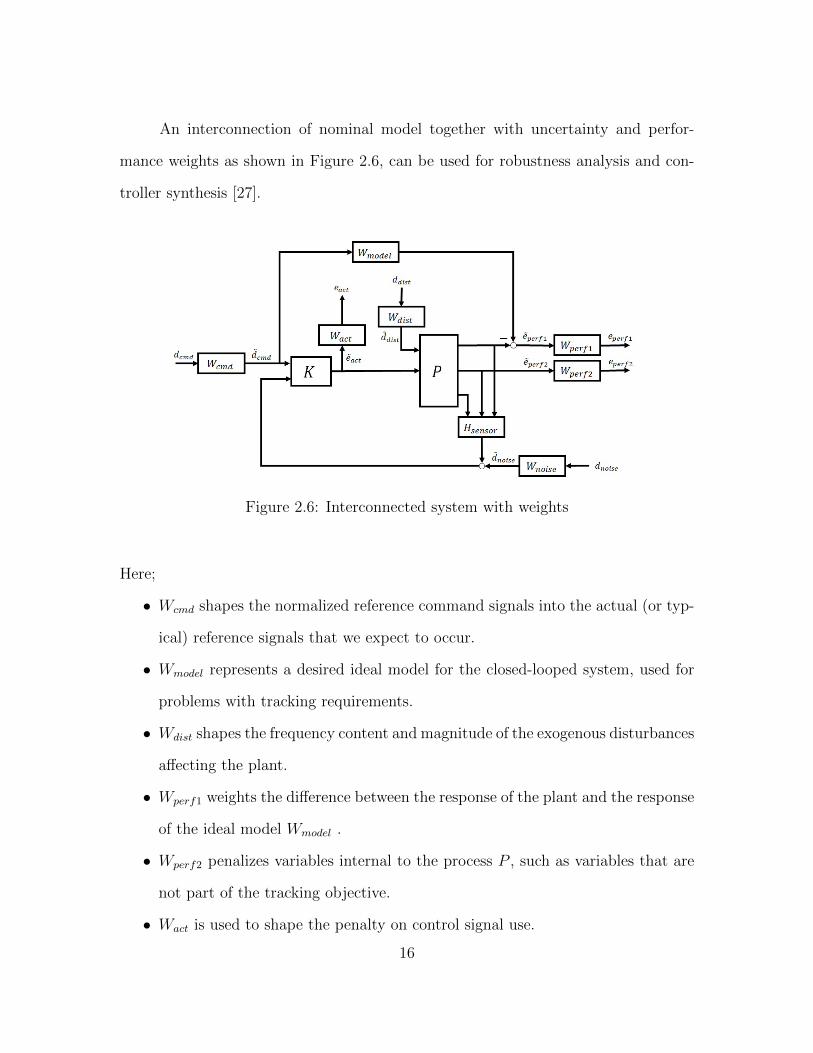
An interconnection of nominal model together with uncertainty and perfor-
mance weights as shown in Figure 2.6, can be used for robustness analysis and con-
troller synthesis [27].
Figure 2.6: Interconnected system with weights
Here;
• Wcmd shapes the normalized reference command signals into the actual (or typ-
ical) reference signals that we expect to occur.
• Wmodel represents a desired ideal model for the closed-looped system, used for
problems with tracking requirements.
• Wdist shapes the frequency content and magnitude of the exogenous disturbances
affecting the plant.
• Wperf1 weights the difference between the response of the plant and the response
of the ideal model Wmodel .
• Wperf2 penalizes variables internal to the process P , such as variables that are
not part of the tracking objective.
• Wact is used to shape the penalty on control signal use.
16

• Wnoise represents frequency domain models of sensor noise.
• Hsensor represents a model of sensor dynamics.
2.2.4 Linear Fractional Transformation (LFT)
An uncertain system can be represented in a linear fractional transformation
(LFT) form, where M is the nominal model together with uncertainty and perfor-
mance weights for analysis problems and ∆ is a block diagonal matrix with different
types of uncertainties as the block diagonal elements. Here, the controller is also
absorbed in M .
Figure 2.7: Upper connected model
Here;
d shows the exogenous disturbances,
e shows the regulated variables, i.e., errors.
The system can simply be written as: z
e
= M
w
d
; w = ∆z
and the transfer function M can be partitioned as:
M =
M11(s) M12(s)
M21(s) M22(s)
17

Selecting ∆ such that the set of equations is well posed and the vectors e and d are
related by:
e = Fu(M,∆)d
where;
Fu(M,∆) = M22 +M21∆(I −M11)−1M12 (2.2)
Fu is called an upper linear fractional transformation (LFT) of M with ∆.
Likewise, a feedback loop can be represented in a linear fractional transfor-
mation (LFT) form, where P is the nominal model together with uncertainty and
perfromance weights and K is an LTI system with its own states for output feedback
control.
Figure 2.8: Lower connected model
Here;
u shows the manipulated variables, i.e., controls,
y shows the sensed variables, i.e., measurements.
The plant dynamics can be written as:x
e
y
=
A B1 B2
C1 D11 D12
C2 D21 D22
x
d
u
=
P11 P12
P21 P22
x
d
u
18

where;
P11 = [A] ; P12 =
[B1 B2
]; P21 =
C1
C2
; P22 =
D11 D12
D21 D22
and for the controller dynamics; xK
u
= K
xK
y
where;
K =
AK BK
CK DK
Similarly, the transfer function from inputs to outputs when lower loop is closed with
K is:
Fl(P,K) = P11 + P12K(I − P22K)−1P21 (2.3)
This is called a lower linear fractional transformation (LFT) [28]. The overall system
can be represented as the connection of lower and upper LFT models as shown in
Figure 2.9.
Figure 2.9: Overall system
19

2.2.5 Stability and Performance
Considering the system shown is Figure 2.9;
• Nominal stability refers to the property that the closed-loop system is stable
for one model at the center of the model set, i.e. ∆(s) = 0.
• Nominal performance refers that, in addition to stability, the nominal closed-
loop system should satisfy the performance requirements.
• Robust stability refers the property that the closed-loop system is stable for all
stable ∆ where ‖∆‖∞≤1, i.e. the controller must stabilize all plants defined by
the uncertainty description Fu(P,∆).
• Robust performance refers that, the performance specifications should be satis-
fied by the closed-loop system for all plants defined by the uncertain description
[29].
2.2.6 Robustness Measures
In classical control, robustness is ensured by providing sufficient gain and phase
margins to counteract the effects of inaccurate modeling or disturbances. In terms
of the Bode magnitude plot, it is known that the loop gain should be high at low
frequencies for performance robustness but low at high frequencies, where unmodeled
dynamics may be present, for stability robustness. Classical control design techniques
are generally in the frequency domain, so they afford a convenient approach to robust
design for SISO systems. However, it is well known that the individual gain margins,
phase margins, and sensitivities of all the SISO transfer functions in a multivariable
system have little to do with its overall robustness [15].
Modern control techniques provide a direct way to design multiloop controllers
for MIMO systems by closing all the loops simultaneously. As coupling generally
exists between inputs and outputs of a MIMO system, approaches such as making
20

several individual SISO frequency plots for various combinations of the inputs and
outputs and examining gain and phase margins may not always yield much insight
into the true behavior of the system [15]. However, the classical frequency-domain
robustness measures may easily be extended to MIMO systems in a rigorous fashion
by using the notion of the singular value.
Theorem 2 (Singular Value Decomposition) [29]:
Defining C as the set of complex numbers, let A ∈ Cm×n , there exists unitary
matrices U ∈ Cm×m and V ∈ Cn×n such that:
A = UΣV ∗
where;
Σ = diag(σ1, σ2, . . . , σp, 0)
and;
σ1 ≥ σ2 ≥ · · · ≥ σp ≥ 0, p = min(m,n)
σ(A) = σmax(A) = σ1; the largest singular value of A
σ(A) = σmin(A) = σp; the smallest singular value of A
The multivariable Bode magnitude plot, which is the plot of the singular values
of the transfer function matrix versus frequency, allows the experience of classical
control theory to be applied to MIMO systems. Analogous to SISO counterpart, in a
coupled MIMO system the minimum singular value of the loop gain should be large
at low frequencies for robust performance and the maximum singular value of the
loop gain should be small at high frequencies for robust stability [15].
2.2.7 Structured Singular Value - µ
The structured singular value is a straightforward generalization of the singular
values for constant matrices.
21

Figure 2.10: Standard feedback interconnection
Considering the standard feedback interconnection as shown in Figure 2.10,
with stable M(s) and ∆(s), the question is: how large ∆ can be, in the sense of
‖∆‖∞, without destabilizing the feedback system? It is known that the feedback
system will become unstable if det(I −M∆) = 0 for some s ∈ C. Defining α > 0
such that the closed-loop system is stable for all stable ‖∆‖∞ < α, the maximum
value of this α, αmax is called the robust stability margin. From small gain theorem:
1
αmax= ‖M‖∞ = max
s∈Cσ(M(s)) = max
ωσ(M(jω))
where;
σ(M(s)) =1
min {σ(∆) : det(I −M∆) = 0, ∆ is unstructured}
To quantify the smallest destabilizing structured ∆ the concept of singular values is
generalized. Defining structured singular value:
µ∆(M(s)) =1
min {σ(∆) : det(I −M∆) = 0, ∆ is structured}
which is the largest structural singular value of M(s) with respect to the structured
∆, and,
1
αmax= max
s∈Cµ∆(M(s)) = max
ωµ∆(M(jω))
for structured uncertainty [29]. An exact solution for µ does not exist. A solution
can be approximated via upper and lower bounds on µ. The method of approxima-
tion depends on the structure of the ∆ block [28]. The structured singular value µ
22

can be used to evaluate the robustness margins for a linear system with structured
uncertainty as shown in Figure 2.7.
Theorem 3 (Robust stability) [28]:
Remembering the upper LFT definition in (2.2), robust stability can be defined
as:
∀∆, Fu(M,∆) is stable iff supωµ(M11(jω)) ≤ 1 , 0 ≤ ω ≤ ∞
This theorem provides a test for the stability of the system for all allowable
perturbations. Usually stability is not the only property of a feedback system that
must be robust to perturbations. The effect of disturbances on the error signals can
increase greatly and performance may degrade significantly when the nominal model
is perturbed. A robust performance test is necessary to indicate the worst case level
of performance associated with a given level of perturbations.
The robust performance problem can be formulated as a robust stability prob-
lem by associating a fictitious full block of uncertainty ∆perf , with the performance
inputs and outputs. The robust performance problem is equivalent to a robust sta-
bility problem but with respect to a different block structure. Consider a new ∆
structure defined as:
∆ =
∆ 0
0 ∆perf
; ∆perf∈Cnv×ne
Robust performance is defined by the following theorem.
Theorem 4 (Robust performance) [28]:
Robust performance is defined by:
∀∆, Fu(M,∆) is stable and ‖Fu(M,∆)‖∞ < 1 iff supωµ∆(M(jω)) ≤ 1 , 0 ≤ ω ≤ ∞
23

This means that performance robustness of a closed-loop system can be evalu-
ated by a µ test across all frequencies. The peak value on the µ plot determines the
robustness properties.
2.3 µ-Synthesis
Structured singular value (µ) synthesis is a multivariable design method that
can be used to directly optimize robust performance [9]. Performance specifications
are defined as weighted transfer functions that describe magnitude and frequency con-
tent of external disturbances, pilot commands, atmospheric gusts, and sensor noise,
as well as allowable magnitude and frequency content of generalized tracking errors,
handling qualities, ride qualities, and actuator activity [9][27]. Specifications of per-
formance and definition of the model set over which performance must be achieved are
all incorporated into a single standard interconnection structure, upon which existing
design algorithms can operate [9].
The µ-synthesis design technique combines the H∞ control design with µ-
analysis. Considering the standard robust performance µ-analysis framework, the
overall system structure (Figure 2.9) and Theorem 4, it is desired to find a controller
K achieving:
infstabilizing K
supω{Fl(P (jω), K(jω))}
This minimization does not have a closed form solution. Upper bounds defined for
complex µ can be used to approximate the solution. Using this fact the problem can
be put in the following form:
minstabilizing K
{minDω
{maxω
σ[DωFl(P,K)(jω)D−1
ω
]} }or equivalently;
minstabilizing K
{minDω
∥∥DωFl(P,K)(jω)D−1ω
∥∥∞
}24

The approach used in solving this problem is to minimize the above expression for
either K or D while holding the other constant. For fixed D it becomes an H∞
optimal control problem. For K fixed, D can be formulated as a convex optimization
problem. This process is applied iteratively until a satisfactory controller is achieved
[28]. Main steps in µ-synthesis are as follows:
1. Interconnection Structure Definition
2. H∞ Synthesis
3. µ Analysis
4. Rational Approximation of D-Scales
5. D −K Iteration
6. Changing Weights
Interconnection Structure [9][27]:
Figure 2.11: Generic interconnection structure
Interconnection structure is a state-space realization of the aircraft dynamics,
augmented with handling qualities models and weighting functions with various inputs
and outputs that specify control design goals. This structure is later used to define
25

the synthesis problem in the simple LFT form as shown in Figure 2.9. Some of the
constituents of an interconnection structure are as follows:
Aircraft Model
The linear dynamic models of the bare airframe, actuators and the sensors are
the central components of the interconnection structure. As appropriate, some of the
dynamics such as low-frequency states that are not important to the design or high-
frequency states, whose frequencies exceed intended bandwidth of the control loops
may be omitted, truncated or residualized. A time delay in Pade-approximation form
may be included for specific systems.
Figure 2.12: Plant dynamics
Performance Model
This model defines generalized errors e and generalized disturbances d of the
model shown in Figure 2.11. These are the signals to be used to judge the quality
of closed-loop performance. The most common generalized errors are tracking errors
between the outputs of closed-loop system and some reference models, actuator de-
flections and actuator rates. Generalized disturbances are the various external inputs
that excite the feedback loop and drive errors such as external disturbances (gusts,
store drops, gun fire transients, etc.) and commands from pilots or outer loops.
Uncertainty Model
This model defines the set of plants over which performance objectives must be
satisfied. It is represented by signals w and z which connect uncertain components
∆ into the feedback loop. Uncertainties may be defined for inputs and outputs, and
26
for the system parameters. Design models used for flight control typically exhibit
good fidelity at lower frequencies but they degrade rapidly at higher frequencies due
to poorly modeled or neglected effects as aeroelasticity, actuator compliance, servo
dynamics, computational/digital effects. Similar high frequency uncertainties are
also associated with sensor hardware for various measured aircraft outputs. Another
important type of uncertainty is internal to the design model, associated with such
things as mass, inertia and/or aerodynamic coefficients.
Weights
The role of weights is to scale the interconnection structure (i.e., normalize
it) such that control objectives in the unscaled structure are satisfied whenever the
closed-loop gain from d to e in the scaled structure is less than unity for all unit-size
perturbations ∆. The functions associated with signals d and e are called performance
weights whereas those associated with w and z are called uncertainty weights. The
weights are the specifications that drive the control design. They can either be used
to determine achievable performance against fixed specifications or to trade off some
specifications. In this manner, all of the classical control design knobs are embodied
in the size and shape of the weights.
The weights chosen for the tracking errors can be thought of as penalty func-
tions. That is, weights should be large in frequency ranges where small errors are
desired and small where larger errors can be tolerated. Normally it is flat at low fre-
quency and rolls off at high frequency. Often, accurate matching of the ideal model at
low frequency is desired and less accurate matching at higher frequency is required,
which turns out a weighting function which is flat at low frequency and rolls off and
flattens out at a small, nonzero value at high frequency.
Actuator deflection and rate weights are used to penalize larger and faster
deflections and thereby minimize control activity. Their size could be chosen to
27

make the normalized deflection and rate nearly flat and unit-size. Because system
bandwidth is directly related to system response speed, weights on actuator rates can
be used to modulate final bandwidth of the closed-loop system.
The role of weights for commands, disturbances and noise is basically the op-
posite of the role of weights for error. Rather than taking unscaled signals and
normalizing them, these weights take flat unit-size signals and scale them to produce
a specified range of magnitudes and frequencies over which the design must insure
good performance.
Uncertainty weights transform the normalized unit-size perturbations into per-
turbations whose magnitudes and frequency content match uncertainty levels in the
design model. For most aircraft flight control design work, models are reasonably well
known out to the short-period and dutch-roll frequencies. Beyond that, they become
progressively less reliable. Uncertainty weights must reflect this.
Given a normalized interconnection structure, the design problem is to find a
stabilizing compensator K that makes the maximum singular value of the closed-
loop frequency-response matrix from d to e less than unity for all possible unit size
perturbations ∆ with the defined block structure.
∆ =
∆input 0 0
0 ∆output 0
0 0 ∆param
H∞ Synthesis [9]:
This step results in a control compensator K. The closed-loop system is then
formed by connecting the sensors and actuators of P to K to produce the closed-loop
interconnection structure, M .
The problem of finding compensators that make the structured singular value
of M less than unity can be solved by repeated H∞ solutions alternated with rescaling
28

Figure 2.13: Closed-loop interconnection
of the signal sets. This theory provides compensators that minimize the H∞ norm of
M (i.e., minimize the maximum singular value ‘γ’ rather than the structured singular
value ‘µ’, of M over frequency). After the γ search is completed, the final compensator
K is supplied in state-space form. This controller system then used to construct the
closed-loop system M and to compute its frequency response matrix over a frequency
range of interest for subsequent µ-analysis.
µ-Analysis and D-Scales [9]:
This step involves calculation of the structured singular value, µ(M) and its
associated frequency dependent D-scales. The structured singular value provides
a measure of how close the compensator is to meeting its robust performance goals.
Here, a complete point-by-point µ-analysis of closed-loop frequency responseM(jw) is
performed. This involves calculating structured singular values (µ) at each frequency
point and comparing those values against unity.
∆M =
∆input 0 0 0
0 ∆output 0 0
0 0 ∆param 0
0 0 0 ∆p
The block ∆p is the so-called fictitious perturbation representing the perfor-
mance requirements, with input/output signals e and d. For this uncertainty struc-
ture, the condition, µ(M) < 1 ; ∀ω guarantees that closed-loop system M remains
29

stable when ∆ is connected from z to d and ∆p is connected from e to d, simultane-
ously. The latter condition ensures that performance is robust.
The exact value of µ at each frequency is not, in general, easy to calculate, so,
upper and lower bounds are used to bracket the true value. The upper bound, in
particular, is based on a computationally tractable search over the class of scaling
matrices D that commute with perturbution ∆M .
D =
dinIin 0 0 0
0 Doutput 0 0
0 0 Dparam 0
0 0 0 Ip
The specific D’s that achieve the infimum in this equation are called D-scales.
µ(M) ≤ infDσ(DMD−1)
D −K Iteration [9]:
Once the µ-analysis calculations are complete and if the condition µ(M) < 1 is
satisfied throughout the selected frequency band, the current H∞ compensator, K,
meets all robust performance goals. If not, another design iteration is performed until
either an approximately flat µ function across frequency is achieved and/or current
D-scales differ insignificantly from the previous iteration.
If another iteration is appropriate, it differs from the current one only in the
sense that a modified optimization problem, which is a rescaled version of the original
one using the current D-scales as scaling factors, is solved in the H∞ step.
Changing Weights [9]:
If D and K have converged, but the compensator does not meet its goals (i.e.,
µ(M) > 1), then the weights must be changed, trading off some goals against others,
30

Figure 2.14: Feedback system with D-Scales
and then D − K iteration is repeated. M -analysis can be used to determine which
input/output paths are driving the problem.
2.4 Gain Scheduling
Traditionally, satisfactory performance across the flight envelope can be at-
tained by scheduling gains of local autopilot controllers on a slow variable to yield
a global controller [30]. While gain scheduling is well established as a practical tool
for the design of controllers for nonlinear plants and a number of ad-hoc approaches
[31] to interpolation have been reported, very few publications on detailed analyses
of gain scheduled multivariable controllers appear in the literature. Some reported
ad-hoc approaches include [11][17]:
• linearly interpolating poles, zeros, and gains of controller transfer functions;
• linearly interpolating the solutions of Riccati equations in H∞ controller syn-
thesis;
• linearly interpolating the balanced controller realizations of state-space matri-
ces;
• implementing the controllers in parallel and linearly interpolating their output
signals.
All these methods usually give satisfactory results in some particular applica-
tions, however, can generate non stabilizing controllers in other cases [11][19][32]. In
31

addition to ad-hoc interpolation, some theoretically justified methods have also been
presented, such as stability preserving interpolation for feedback gains [11] and lin-
ear parameter varying (LPV) control design methods [11][31][32]. Various synthesis
methods for gain scheduling using linear fractional transformations (LFTs) [33][34][35]
have also been developed. The idea behind this is to let the controller have access to
some of the uncertainties of the system to be controlled [34]. Here, the interpolation
problem is addressed implicitly in that the controllers are also parameter varying [11].
The complexity of the gain scheduling is highly dependent upon the structure
of the LTI controllers at each fixed operating point. With classical control techniques,
the structure of the LTI controller dynamics may be fixed for each operating point
with only few gains varying with changing parameters. However, for multivariable
state space design procedures each LTI controller may have a different state order
and feedback topology. In this latter case, the gain scheduling implementation con-
siderations may become a serious drawback to the use of these multivariable design
approaches [17][36].
In this study two different scheduling approaches will be investigated in detail.
But before that, a prelude on uncertain model representation for a collection of LTI
systems will be given.
Uncertain Model Representation:
In aerospace applications, it is common practice to represent plant dynamics
as a collection of LTI systems, where, each one of the systems correspond to aircraft
dynamics in the neighborhood of a specific operating point. Following this approach,
we define the set of operating points as Λ = {ρ1, . . . , ρn}, where ρi represents a
vector of parameters to be used for scheduling. Then, LTI system matrices can be
32

parameterized by ρi, such that: Ai = A(ρi), Bi = B(ρi), Ci = C(ρi) and Di = D(ρi)
The nonlinear plant dynamics for each operating point becomes:
x = Aix+ Biu
y = Cix+ Diufor each ρi∈Λ
We define the matrix polynomials:
PA(δ) =n−1∑i=0
Aiδi; PB(δ) =
n−1∑i=0
Biδi; PC(δ) =
n−1∑i=0
Ciδi; PD(δ) =
n−1∑i=0
Diδi
with proper transformation from Ai, Bi, Ci, Di to Ai, Bi, Ci, Di, where, δ ∈ [−1, 1],
such that at the points {δj}nj=1 we have PA(δj) = Aj ; PB(δj) = Bj ; PC(δj) = Cj and
PD(δj) = Dj ; j = 1, . . . , n .
At this point it is possible to define the matrix M , which represents the system
dynamics using matrices Ai, Bi, Ci, Di such that:
M =
A0 B0 A1 B1 · · · An Bn
C0 D0 C1 D1 · · · Cn Dn
I 0 0 0 · · · 0 0
0 I 0 0 · · · 0 0
0 0 I 0 · · · 0 0
0 0 0 I · · · 0 0
0 0 0 0 · · · 0 0
0 0 0 0 · · · 0 0
with δI as the structured uncertainty associated with the gain scheduled plant. Now
it is possible to treat the system in a standard LFT form as displayed in Figure 2.15.
A quiet similar approach for obtaining LPV models can be found in Ref. [18].
Synthesis using Simplified LPV Model [10]:
Once the plant is scheduled using the uncertainty loop as explained in the pre-
vious chapter, the very same uncertain parameters can also be used for controller
33

Figure 2.15: LFT form with scheduled plant
synthesis. For a linear parameter varying (LPV) plant, which is generated using a
number of LTI systems, a single controller can be synthesized by D − K iteration
provided that the controller input signals is arranged in a proper fashion in intercon-
nection structure.
For a plant composed of two LTI systems, the controller is also desired to
act as a twofold system compatible with the plant. For this, the input channels of
the controller is modified in order that the two input channels are multiplied with
uncertain gains k1 and k2 to provide two linearly interpolated signals, e.g.:
for − 1 ≤ δ ≤ 1; k1 = (1− δ)/2; k2 = (1 + δ)/2
A graphical representation for linear interpolated simplified LPV model is given
in Figure 2.16. A detailed discussion on this method can be found in Ref. [10].
The method can be extended to higher order LPV plants. In Figure 2.17, a
second order LPV model composed of three LTI systems is taken into consideration.
In this case, three input channels are multiplied with uncertain gains k1, k2 and k3
where;
for − 1 ≤ δ ≤ 1; k1 = δ(δ − 1)/2; k2 = (1− δ2); k3 = δ(δ + 1)/2
Once the system interconnection is built, standard µ-synthesis steps can be
followed for controller synthesis. The resulting LTI controller will have higher di-
34

Figure 2.16: 1st order simplified LPV interconnection
mensions due to increased number of inputs and most likely will be of higher order,
compared to LTI controllers designed for single operating points.
Stability Preserving Interpolation [11][37]:
Synthesis of gain scheduled controllers for nonlinear plants often requires that
a parameter-varying controller be generated from a finite set of linear time-invariant
controllers. The scheduling variable can be a function of the state, input, and exoge-
nous signal. For the generic LTI system representation of the plant Σ:
x
e
y
=
F G1 G2
H1 J11 J12
H2 J21 J22
x
d
u
(2.4)
if the components of this system can be formulated as matrix functions of a parameter
ρ, then the plant Σ(ρ) is also a function of ρ. So the system equations become:
35

Figure 2.17: 2nd order simplified LPV interconnection
Σ(ρ) =
x(t) = F (ρ)x(t) +G1(ρ)w(t) +G2(ρ)u(t)
e(t) = H1(ρ)x(t) + J11(ρ)w(t) + J12(ρ)u(t)
y(t) = H2(ρ)x(t) + J21(ρ)w(t)
(2.5)
Assume that controllers in LTI form, Λi, have been synthesized for selected n operat-
ing points which are also parameterized by ρ, e.g.: Λi = Λ(ρi), for i = 1, . . . , n. The
equations of the LTI controllers to be interpolated can be written as:
Λi =
z(t) = Aiz(t) +Biy(t)
u(t) = Ciz(t) +Diy(t)(2.6)
The target in stability preserving interpolation is to generate a parametric con-
troller Λ(ρ) which can be used in conjunction with the parametric plant Σ(ρ), and
the closed-loop system is guaranteed to be stable for any ρ. For this to be possible,
stability covering condition [11] should be satisfied for all Λi and Σ(ρ). The steps
followed in this process is briefly displayed in Figure 2.18.
36

Figure 2.18: Steps of stability preserving interpolation
The process is simply based on an intermediate layer J (ρ), and parameteriza-
tion of pointwise controllers Λi by use of this new layer. In the following, a linear
interpolation between two operating points ρ1 and ρ2 is assumed with ρ1 = 0, ρ2 = 1
and ρ ∈ (0, 1). Defining the closed-loop system using lower LFT of the plant Σ(ρ)
and the controller Λi:
Fl(Σ(ρ),Λi) =
x(t) = Ai(ρ)x(t) + Bi(ρ)u(t)
y(t) = Ci(ρ)x(t) + Di(ρ)u(t)(2.7)
Lemma: Given the LTI controller Λi and the LPV system Σ(ρ) with ρ constant,
suppose there exists K and L such that F (ρ)+G2(ρ)K and F (ρ)+LH2(ρ) are stable.
Then Λi has the same transfer function as Fl(J (ρ),Qi(ρ)) where;
J (ρ) =
x(t) = (F (ρ) +G2(ρ)K + LH2(ρ))x(t)− Lw(t) +G2(ρ)u(t)
e(t) = K(ρ)x(t) + u(t)
y(t) = H2(ρ)x(t)− w(t)
(2.8)
Qi(ρ) =
z(t) = Ai(ρ)z(t) + Bi(ρ)y(t)
u(t) = Ci(ρ)z(t)(2.9)
37

with;
Ai(ρ) =
F (ρ) +G2(ρ)DiH2(ρ) G2(ρ)Ci
BiH2(ρ) Ai
(2.10)
Bi(ρ) =
L(ρ)−G2(ρ)Di
Bi
(2.11)
Ci(ρ) =
[−K(ρ) +DiH2(ρ) Ci
](2.12)
Di(ρ) = −Di (2.13)
where A1(ρ) and A2(ρ) both stable for ρ ∈ (0, 1). Proof of this Lemma can be found
in Ref. [37]. Let W1(ρ) and W2(ρ) be symmetric positive definite matrices such that:
AT1 (ρ)W1(ρ) +W1(ρ)A1(ρ) < −Ifor ρ ∈ [a, 1) (2.14)
AT2 (ρ)W2(ρ) +W2(ρ)A2(ρ) < −Ifor ρ ∈ (0, b] (2.15)
This yields,
(1−ρ)(AT1 (0)W1(0) +W1(0)A1(0)
)+ρ(AT2 (1)W2(1) +W2(1)A2(1)
)< −I; for ρ ∈ (0, 1)
Defining:
W (ρ) = (1− ρ)W1(0) + ρW2(1) (2.16)
AW (ρ) = W−1(ρ)((1− ρ)W1(0)A1(0) + ρW2(1)A2(1))
is stable for each ρ ∈ (0, 1).
38

Defining:
W (ρ) =
W1(ρ), ρ ∈ [a, 0]
W (ρ), ρ ∈ (0, 1)
W2(ρ), ρ ∈ [1, b]
(2.17)
A(ρ) =
A1(ρ), ρ ∈ [a, 0]
AW (ρ), ρ ∈ (0, 1)
A2(ρ), ρ ∈ [1, b]
(2.18)
B(ρ) =
B1(ρ), ρ ∈ [a, 0]
(1− ρ)B1(0) + ρB2(1), ρ ∈ (0, 1)
B2(ρ), ρ ∈ [1, b]
(2.19)
C(ρ) =
C1(ρ), ρ ∈ [a, 0]
(1− ρ)C1(0) + ρC2(1), ρ ∈ (0, 1)
C2(ρ), ρ ∈ [1, b]
(2.20)
D(ρ) =
D1(ρ), ρ ∈ [a, 0]
(1− ρ)D1(0) + ρD2(1), ρ ∈ (0, 1)
D2(ρ), ρ ∈ [1, b]
(2.21)
then
Q(ρ) =
z(t) = A(ρ)z(t) + B(ρ)y(t)
u(t) = C(ρ)z(t) + D(ρ)y(t)(2.22)
is a stable system for each ρ ∈ [a, b] ; and Λ(ρ) = F l(J (ρ),Q(ρ) stabilizes Σ(ρ) for
each ρ ∈ [a, b]. For Wi(ρ) and W−1i (ρ), partitioned as follows:
Wi(ρ) =
Si(ρ) Ni(ρ)
NTi (ρ) Pi(ρ)
; W−1i (ρ) =
Ri(ρ) Mi(ρ)
MTi (ρ) Qi(ρ)
(2.23)
39

Defining:
Li(ρ) = G2(ρ)Di − S−1i (ρ)Ni(ρ)Bi (2.24)
Ki(ρ) = DiH2(ρ) + CiMTi (ρ)R−1
i (ρ) (2.25)
and;
L(ρ) =
L1(ρ), ρ ∈ [a, 0)
S−1(ρ)((1− ρ)S1(ρ)L1(ρ) + ρS2(ρ)L2(ρ)), ρ ∈ [0, 1]
L2 (ρ) , ρ ∈ (0, b]
(2.26)
K(ρ) =
K1(ρ), ρ ∈ [a, 0)
((1− ρ)K1(ρ)R1(ρ) + ρK2(ρ)R2(ρ))R−1(ρ), ρ ∈ [0, 1]
K2(ρ), ρ ∈ (0, b]
(2.27)
where
S(ρ) = (1− ρ)S1(ρ) + ρS2(ρ) (2.28)
R(ρ) = (1− ρ)R1(ρ) + ρR2(ρ) (2.29)
A more detailed explanation of the method can be found in Ref. [11] and Ref. [37].
A step by step implementation will be discussed in Chapter 4.
40

CHAPTER 3
CONTROL ALLOCATION
3.1 Background
The control algorithm hierarchy for over actuated systems with a redundant
set of effectors commonly includes three levels. First, a high level control algorithm
commands a vector of virtual control efforts (i.e. forces and moments) in order to
meet the overall control objectives. Second, a control allocation algorithm coordinates
the different effectors such that they together produce the desired virtual control
efforts, if possible. Third, low-level control algorithms may be used to control each
individual effector via its actuators [38]. So to say, control allocation deals with the
problem of distributing a given control demand among an available set of actuators
[39]. Control allocation offers the advantage of a modular design where the high-level
control algorithm can be designed without detailed knowledge about the effectors and
actuators. Important issues such as input saturation and rate constraints, actuator
and effector fault tolerance, and meeting secondary objectives such as power efficiency
are handled within the control allocation algorithm [38].
Figure 3.1: Control hierarchy for over-actuated systems
41

A typical control hierarchy diagram for over actuated systems is shown in Fig-
ure 3.1. Here;
r shows the reference commands for control law,
y shows the measurable output parameters,
x shows the controller feedback signals,
v shows the virtual control command generated by the control laws, and
u shows the true control input to the control effectors.
The control allocation problem is defined as finding an exact or approximate
solution for a system of linear equations subject to constraints for redundant actu-
ator control variable commands. The constraints usually arise from actuation rate
and position limits [40]. This is often posed as a constrained least squares problem to
incorporate the actuator position and rate limits. Most proposed methods for real-
time implementation only deliver approximate, and sometimes unreliable solutions
[13]. An axis priority weighting can be introduced when the equations cannot be
solved exactly because of the constraints. Likewise, an actuator command preference
weighting and preferred values can be introduced to uniquely solve the equations
where there are more unknowns than equations [40]. The cost functions can be opti-
mized in real time, or alternatively, pre-computed effector solutions that are optimal
for specific conditions can be used as preferred solutions [12]. Concerns about max-
imum effector-induced loads, as well as repeated load applications causing fatigue
failures may be decisive in determination of this cost function. When some effectors
are slower than others, it may be desirable to use them less often by biasing the
weighting matrix used in the cost function [12]. A variety of approaches for on-line
control allocation have been reviewed in Refs. [38][41][42].
42
3.2 Actuator Constraints
Linear control design is typically carried out without regard to what the system
behavior will be when an actuator is saturated or rate-limited. The gains of the
control loop are selected so that actuators are sufficiently utilized to meet normal
closed-loop performance requirements. Selecting the gains to avoid saturating the
actuators when large disturbances or commands act on the closed-loop would give
poor performance under normal operating conditions. Multivariable systems present
much more of a problem when actuators saturate because the loop-gain has both
magnitude and direction which are both affected by saturating actuators. The loss
in directionality can mean loss of decoupling between the controlled outputs [17]. A
control allocation scheme, in this context, eases handling of saturated actuators in
an over actuated system. As the control law design relies on the limits of virtual
controls, not the individual actuators, the position or rate limit requirements of the
system can simply be embedded in this virtual controls, having a much reduced
impact on controller performance. So, in case of a saturation, the virtual commands
generated by the control laws can be realized by some combination of control surfaces
different than the unsaturated case.
Actuator failures have damaging effect on the performance of control systems,
leading to undesired system behavior or even instability. For system safety and re-
liability, the compensation of actuator failures is of both theoretical and practical
significance. Several design approaches have been studied for this purpose, such as:
multiple-model designs (switching and tuning designs), fault-diagnosis-based designs,
robust control designs, and adaptive designs [43].
In multiple-model designs employed for reconfigurable flight control, it is as-
sumed that the plant belongs to a set of plant models with corresponding set of
controllers. When some actuators fail, a switching mechanism will find the best
43

matched model and switch to the appropriate controller. For fault-diagnosis-based
designs, in addition to a controller, there is an FDI (fault detection and isolation) unit.
When actuator failures appear, a reconfigurable controller will change its structure
and parameters according to the fault diagnosis result to accommodate actuator fail-
ures. In adaptive designs, as the controller is implemented with unknown parameters,
these parameters are updated on-line by some adaptive laws in the case of actuator
failures. Robust control designs for systems with actuator failures use robust control
techniques to accommodate some classes of failures by treating them as uncertainties.
Most existing control designs for systems with actuator failures either are based on
some knowledge of actuator failures or depend on some extra detection techniques
[43].
For aircraft with redundant control effectors, it is much easier to overcome
the effects of an actuator failure by implementing a control allocation based con-
trol method. A control allocation algorithm will simply use whatever controls are
functional to attempt to satisfy the demands [12].
3.3 Control Allocation Problem
In most aerospace applications, control effectors are used to change the aero-
dynamic moments - and less frequently the aerodynamic forces - acting on the body.
As discussed above, all control effectors have certain position limits, usually specified
as positive and negative deflections from a specified position that is taken as zero de-
flection, and limits on the rate they can travel. Normally the actuator dynamics are
very fast compared to the responses of the airplane [12]. The basic control allocation
problem can be formulated as:
44

For given B, υ, u, u, find u such that:
Bu = υ, u ≤ u ≤ u
where;
υ is the vector of desired moments or virtual commands and υ ∈ Rn. This vector
is not always defined as actual moments, however this does not affect the geometry
of the problem or methods of its solution.
u is vector of control effectors, u ∈ Rm, where m > n and B is the control
effectiveness matrix, B ∈ Rn×m
The set of equations is under-determined and mathematically has an infinite
number of solutions. When control limitations are introduced the equations may have
no solutions. If there is an admissible control vector for a particular moment, then
that moment is said to be attainable [12]. There are several published methods for
handling the control allocation problem.
Ganging [12]:
Individual control effectors can be interconnected so that the movement of one
depends on that of another. This interconnection reduces the number of independent
solutions in control allocation problem, e.g. if m − n interconnections are applied,
the problem becomes determined and can be solved by simply inverting B.
Generalized Inverses [12]:
A generalized inverse is taken to be a matrix P that, without regard to the
limits on control effectors, finds:
up = Pυ
such that Bup = υ, and BP = In. All such generalized inverses may be represented
as:
P = N(BN)−1 (3.1)
45

where N is arbitrary with N ∈ Rm×n and BN is invertible.
Daisy Chaining [12]:
The method works by dividing the controls into two or more groups based on
the frequency of use of effectors. The first group, typically the more conventional
control effectors, are to be used most frequently. The subsequent groupings are to be
used only if the set of previous groupings is unable to satisfy the moment demand.
Direct Allocation [12][38][44]:
Direct Allocation is a constrained control allocation approach based on some
scaling of the unconstrained optimal control allocation, such that the resulting control
allocation is projected onto the boundary of the set of attainable moments (AMS).
In simple terms, AMS is defined as the domain of all attainable virtual controls
(moments) using every admissible control (effector) for a given control effectiveness
matrix B. The Direct Allocation method finds a one-to-one relation between an
actuator command and the controller (virtual) command using the boundary of the
AMS. The information from AMS boundary can be converted to a set of look-up
tables, so that, the computational burden is reduced considerably, which makes it
suitable for on-line applications.
Optimization Based Allocation [38]:
The presence of physical constraints, operational constraints and secondary ob-
jectives makes optimization-based design a powerful approach. The simplest formu-
lations allow explicit solutions to be computed using numerical linear algebra, while
the more challenging formulations with complex constraints and objectives call for
iterative numerical optimization procedures.
A powerful approach is to explicitly minimize the cost J defined as the n-norm
of the weighted error between the allocated control input, u, and the desired one, up,
i.e.: find minuJ where J = ‖W (u− up)‖n with constraints u ≤ u ≤ u.
46
With the cost function defined using either 1-norm or ∞-norm, this resulting
problem is a linear program (LP) that can be solved using iterative numerical LP
algorithms. With the common choice of 2-norm, the control allocation problems
leads to a quadratic program (QP) that can be solved using numerical QP methods.
Dynamic Allocation [39]:
Dynamic control allocation is a method proposed for distributing the control
effect in the frequency domain and thus using the redundancy to have different actu-
ators operate in different parts of the frequency spectrum. This requires the mapping
from υ to u to depend also on earlier values of u and υ. A frequency-dependent
control distribution can be designed to account for different actuator bandwidths by
extending regular control allocation by also penalizing the actuator rates.
In this study two different control allocation approaches will be investigated
in more detail. First, a simple method, Cascaded Generalized Inverses, then a more
complicated, Weighted Least Squares based algorithm will be implemented. Both
will be tested in an integrated simulation using a number of scenarios with several
maneuvers and malfunctions and their performance will be compared.
Cascaded Generalized Inverse (CGI) [12]:
In its simplest form, CGI method uses a single generalized inverse exclusively
until one or more of the control effectors is commanded to a position beyond satura-
tion. When this happens, the saturated controls are left at whatever limit they were
when saturated and removed from the problem. The control allocation process is
repeated with the reduced problem until desired moments are satisfied or no control
effectors are left to allocate.
Weighted Least Squares (WLS) [13]:
In a constrained optimization framework, the basic control allocation problem
can be stated as finding the control that minimizes the weighted error between the
47
preferred and actual solution which is in a set of feasible solutions that minimize the
weighted deviation from the virtual control, i.e.:
minu∈K‖Wu(u− up)‖
where
K = minu≤u≤u
‖Wυ(Bu− υ)‖
An approximate way to reformulate the problem is to merge the two optimization
criteria into one by summation and form a weighted least squares problem:
minu≤u≤u
(‖Wu (u− up) ‖2 + γ‖Wυ(Bu− υ)‖2) (3.2)
The most frequently encountered approaches for solving this problem are based
on constrained quadratic programming. Active set methods are used in many of
today’s solvers for constrained quadratic programming, and can be shown to find the
optimal solution in a finite number of iterations. We will implement an active set
algorithm based solver for this weighted least squares problem.
48
CHAPTER 4
CASE STUDY
4.1 Background
A tailless configuration presents challenges in various disciplines, stability and
control being the most prominent [4]. Major discrepancies related to this config-
uration are: light short-period damping, sensitive pitch control, inefficient use of
high-lift devices, difficulty in takeoff rotation, lack of directional stability, poor di-
rectional control and strong coupling between control effectors [6][7]. Some of the
proposed solutions for these were using wings with reflexed airfoil shapes, selecting
proper combination of sweepback, taper and twist, inserting flow separators on wings,
ganging controls in a proper way, etc. [6]. These, by no doubt, helped improving the
designs, but frequently, they also created new problems or caused degradation in flight
performance, so tailless design is understood not to be a simple task.
Today, one may be puzzled by the fact that we see so few tailless aircraft. This
is not simply a reflection of aircraft manufacturers’ conservatism, but an indication
of the fact that tails are an efficient means of satisfying the requirements for trim and
control. It is very easy to design a very bad tailless aircraft while conventional design
wisdom leads to a quite good conventional design [45].
Available literature on tailless configurations may be categorized into three ma-
jor groups: aircraft design oriented, control system design oriented and aerodynamic
analysis oriented works. A selection from the literature, which are considered to be
interesting by the author, will be presented here:
49

Ref. [46] is one of the earliest attempts to compile and describe all the special
problems of tailless aircraft with an engineering perspective. The main focus is on de-
sign considerations and flight characteristics. Only the aerodynamic aspects of tailless
aircraft are considered with a special attention to Horten gliders. Ref. [47] intends to
assess the handling qualities of a tailless configuration, using piloted-handling trials in
a moving-base simulator and to determine the effect of simulator motion on handling-
quality ratings. Ref. [6] is concerned with identifying and then evaluating the flight
dynamics, stability, flight controls and handling qualities of a generic Blended Wing
Body (BWB) large transport aircraft concept. The possibility to use the conventional
flying and handling qualities criteria and requirements for FCS design for BWB con-
figuration is investigated. Ref. [48] deals with a very special kind of tailless aircraft:
hang gliders. Some analytical methods and tools are developed for a quantitative
understanding of hang glider aerodynamics. Effects of flexibility is investigated by
combined aerodynamic and structural analysis. Wind tunnel tests are performed us-
ing elastically scaled model, for verification. Ref. [3] investigates the basic problems
related to the development of advanced large-capacity aircraft of a flying-wing (FW)
configuration from a TsAGI perspective. Ref. [1] discusses the proper incorporation
of yaw control power effects - their magnitude and bandwidth - within the iterative
conceptual design process, which is considered to be critical to a successful aircraft
design from a dynamics standpoint. It also covers other factors that must be ac-
counted for in designing tailless aircraft. Ref. [49] presents a numerical approach for
determining optimum lift distribution for tailless aircraft using multiple trailing-edge
flaps such that drag is minimized with a pitching-moment constraint.
The purpose of Ref. [50] is to determine the tailless aircraft performance im-
provements gained from relaxed static stability, to quantify this potential in terms of
range-payload improvements, and to identify other possible operational and handling
50

benefits or problems. Two configurations are studied: a high aspect ratio, short-chord
wing proposed as a high-altitude long endurance class UAV, and a lower aspect ratio,
high volume wing proposed for a manned long-range reconnaissance mission. Ref. [42]
presents a direct adaptive reconfigurable flight control approach and demonstrates its
effectiveness via an application to an advanced tailless fighter aircraft. The recon-
figurable control law is based on a dynamic inversion controller in an explicit model
following architecture and an on-line neural network is used to adaptively regulate the
error between the desired response model and the actual vehicle response. Ref. [41]
investigates an eigenstructure assignment based flight control system for a wind tun-
nel model of a tailless aircraft and proposes a novel method capable of maintaining
stability, desired performance, and disk gain/phase margins under control effector
failures. In Ref. [4], a reconfigurable sliding mode flight controller is designed for
a tailless jet fighter. The controller achieves robust, high accuracy command angle
tracking both before and after damage. An optimal control allocation algorithm is
employed using nominal mathematical model of an aircraft. Ref. [51] describes a neu-
ral network based direct adaptive control approach to the problem of reconfigurable
flight control. A tailless fighter aircraft configuration with multiple and redundant
control actuators is used to illustrate the level to which handling qualities can be
maintained in the presence of large scale failures in the actuation channels.
Ref. [52] is focused on the use of active flow control on a tailless aircraft model.
Wind tunnel experiments are performed to test the effectivity of sweeping jet flow
control for the longitudinal stability problems at higher incidence angles. Ref. [53]
intends to use computational fluid dynamics to study the tumbling characteristics of
a tailless aircraft and then determine dynamic stability information from the simula-
tions. The effects of various parameters are investigated and lumped pitch damping
derivatives are determined from the simulations. Ref. [54] evaluates the stability
51
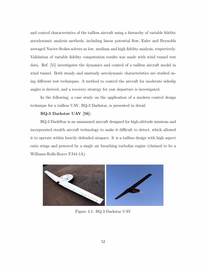
and control characteristics of the tailless aircraft using a hierarchy of variable fidelity
aerodynamic analysis methods, including linear potential flow, Euler and Reynolds
averaged Navier-Stokes solvers as low, medium and high fidelity analysis, respectively.
Validation of variable fidelity computation results was made with wind tunnel test
data. Ref. [55] investigates the dynamics and control of a tailless aircraft model in
wind tunnel. Both steady and unsteady aerodynamic characteristics are studied us-
ing different test techniques. A method to control the aircraft for moderate sideslip
angles is derived, and a recovery strategy for yaw departure is investigated.
In the following, a case study on the application of a modern control design
technique for a tailless UAV, RQ-3 Darkstar, is presented in detail.
RQ-3 Darkstar UAV [56]:
RQ-3 DarkStar is an unmanned aircraft designed for high-altitude missions and
incorporated stealth aircraft technology to make it difficult to detect, which allowed
it to operate within heavily defended airspace. It is a tailless design with high aspect
ratio wings and powered by a single air breathing turbofan engine (claimed to be a
Williams-Rolls-Royce FJ44-1A).
Figure 4.1: RQ-3 Darkstar UAV
52

The first prototype made its first flight on March, 1996. Its second flight ended
in a crash shortly after takeoff. A modified, more stable design (the RQ-3A) first flew
on June, 1998, and made a total of five flights before the program was canceled.
General characteristics of the vehicle are summarized in Table 4.1.
Table 4.1: RQ-3 basic characteristics [56]
Characteristic Imperial Metric
Length 15 ft 4.57 mWingspan 69 ft 21.03 mHeight 3.5 ft 1.07 mEmpty weight 4360 lb 1980 kgGross weight 8500 lb 3860 kgThrust 1900 lbf 8.5 kNCruise speed 250 kts 464 km/hRange 500 nmi 925 kmService ceiling 45000 ft 13700 m
Since very limited public data is available for the aircraft, some design param-
eters such as wing twist, incidence angle and wing airfoil have been selected by the
author in order to introduce a reasonable design. Instead of the existing control ef-
fectors of RQ-3, in this study, a different set of redundant control effectors is assumed
to be implemented.
4.2 Nonlinear Model
A nonlinear model for RQ-3 has been developed using MATLAB-Simulinkr, to
be used in tasks such as generation of LTI plants for various operating points and
validation of the controllers and control allocation algorithms by simulation. The
aircraft model consists of several sub-models: Atmosphere, flight controls, aerody-
namics, engine, equations of motion, and mass properties [57]. All sub-models are
53

connected to a main data bus, which manages the communication between each other
and input/outputs of the aircraft model. A top level overview of the model is shown
in Figure 4.2.
Figure 4.2: Simulink model overview
Aerodynamic Model [8]:
In conceptual design of an aircraft, the definition of aerodynamic database can
be performed using either analytical, semi-empirical or numerical aerodynamic calcu-
lation techniques. When semi-empirical methods are used within their applicability
limits, remarkable levels of accuracy and short turnaround times are achieved, what
is ideal for conceptual work [58].
Digital DATCOM is an aerodynamic prediction software developed at McDon-
nell Douglas based on the database and systematic methods of USAF Stability and
Control Datcom [59]. It is capable of calculating static and dynamic derivatives as
well as a wide variety of high lift and control device contributions through subsonic,
transonic, supersonic, and hypersonic speed regimes. Its primary purpose is to provide
a rapid estimation of aerodynamic stability and control characteristics. Consequently,
Digital DATCOM is considered to be a convenient tool for the objectives of this study
54
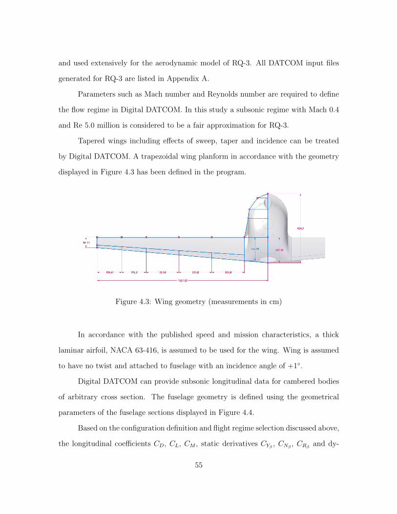
and used extensively for the aerodynamic model of RQ-3. All DATCOM input files
generated for RQ-3 are listed in Appendix A.
Parameters such as Mach number and Reynolds number are required to define
the flow regime in Digital DATCOM. In this study a subsonic regime with Mach 0.4
and Re 5.0 million is considered to be a fair approximation for RQ-3.
Tapered wings including effects of sweep, taper and incidence can be treated
by Digital DATCOM. A trapezoidal wing planform in accordance with the geometry
displayed in Figure 4.3 has been defined in the program.
Figure 4.3: Wing geometry (measurements in cm)
In accordance with the published speed and mission characteristics, a thick
laminar airfoil, NACA 63-416, is assumed to be used for the wing. Wing is assumed
to have no twist and attached to fuselage with an incidence angle of +1◦.
Digital DATCOM can provide subsonic longitudinal data for cambered bodies
of arbitrary cross section. The fuselage geometry is defined using the geometrical
parameters of the fuselage sections displayed in Figure 4.4.
Based on the configuration definition and flight regime selection discussed above,
the longitudinal coefficients CD, CL, CM , static derivatives CYβ , CNβ , CRβ and dy-
55

Figure 4.4: Fuselage sections (measurements in cm)
namic derivatives CLq , CMq , CRp , CYp , CNp , CNr for wing-body combination (wb) are
provided as output by the program. Aerodynamic coefficients for our RQ-3 model,
which are obtained using Digital DATCOM are displayed in Figure 4.5, Figure 4.6
and Table 4.2.
Figure 4.5: Polars for static aerodynamic coefficients
56

Figure 4.6: Polars for aerodynamic damping coefficients
Table 4.2: Fixed aerodynamic coefficients
CYβ -6.08E-03CNβ -4.62E-06CLq -1.66E-01CMq -1.36E-01
High-lift devices such as jet flaps, split, plain, single-slotted, double-slotted,
fowler, and leading edge flaps and slats, control devices, such as trailing-edge flap-type
controls and spoilers, can be analyzed in Digital DATCOM. The program provides the
incremental effects of control device deflections at zero angle of attack. Asymmetrical
deflection of wing control devices can be analyzed for rolling and yawing effectiveness.
In this study, a suite of multiple control effectors consisting of three trailing edge
flaps and two spoilers are assumed to be implemented on each wing. The designation
used for each effector is shown in Figure 4.7.
57

Table 4.3: Control effector designation
No. Effector
1 Inboard flap2 Middle flap3 Outboard flap4 Inboard spoiler5 Outboard spoiler
Figure 4.7: Control effector designation
Effectors 1, 2 and 3 are plain flaps with 30% chord ratio. The deflection limits
are taken as ±25. Effectors 4 and 5 are spoilers located between 65-80% chord on top
surface and maximum projected height of the spoiler is 15% chord, which corresponds
to a 90◦ spoiler angle. Trailing edge down deflection is taken as positive for flaps and
spoiler deflection is taken as negative for convention. Maximum spoiler deflection
is taken as -25 in the model to be in same order of magnitude with maximum flap
deflection.
Figure 4.8: Flap and spoiler configurations
58

Figure 4.9: Change in spoiler angle with spoiler deflection
Table 4.4: Control effector limits
Flap defl. Flap angle Spoiler defl. Spoiler angle
Position (min, max) -25,+25 -25◦,+25◦ -25,0 -90◦,0◦
Rate 60/sec 60◦/sec 100/sec 360◦/sec
Control effectiveness for each of the effectors obtained by Digital DATCOM are
shown in Figure 4.10 and Figure 4.11.
The build-up of the aerodynamic model is briefly explained in the following.
Non-dimensional rotational rates are defined as:
p = pb
2V; q = q
c
2V; r = r
b
2V
The total value for each single aerodynamic coefficient is the sum of clean configura-
tion data and contributions from control surfaces and dynamic derivatives.
59

Figure 4.10: Control effectiveness for flaps and spoilers, CL and CM
Figure 4.11: Control effectiveness for flaps and spoilers, CR and CN
CL = CLwb(α) + CLq wb q +10∑i=1
CLeff (δi) (4.1)
CY = CYβ wbβ + CYp wb(α)p+10∑i=1
CYeff (δi) (4.2)
CD = CDwb(α) +10∑i=1
CDeff (δi) (4.3)
CR = CRβ wb(α)β + CRp wb(α)p+10∑i=1
CReff (δi) (4.4)
CN = CNβ wbβ + CNp wb(α)p+ CNr wb(α)r +10∑i=1
CNeff (δi) (4.5)
CM = CMwb(α) + CMq wb
q +10∑i=1
CMeff(δi) (4.6)
60
Dynamic pressure, angle of attack and angle of sideslip are defined as:
q =1
2ρV 2; α = tan−1(w/u) ; β = sin−1(v/V )
Dimensional forces and moments are:
L = qSCL; D = qSCD; Y = qSCY ; M = qScCM ; N = qSbCN ; R = qSbCR
and body axis aerodynamic forces are:
X = Lsin (α)−Dcos (α)
Z = −Lcos (α)−Dsin (α)
DATCOM methods are known to have limitations in drag calculations and low
accuracy for thick airfoils. Besides, it is seen that parameters such as effects of spoiler
use in wing lift are totally ignored in the program output. As this study is not focused
on the accuracy of the mathematical model, such deficiencies are disregarded as long
as they are considered to have a secondary impact on the derivatives of concern.
Engine Model:
A simplified 2nd order dynamic model based on the more complex engine dy-
namic response characteristics defined in Ref. [60] is used for RQ-3 engine simulation.
A thrust between idle and maximum throttle, Tmax, is assumed to be changing linearly
with throttle position, δthr. The simplified model is:
T = Tmax1.96
s2 + 2.8s+ 1.96(δthr/100)
where 0≤ δthr ≤ 100 and Tmax = 10kN
Flight Controls:
A flight control model composed of a control allocation block and servo dynam-
ics is implemented. Two different control allocation approaches have been tested.
61

A detailed discussion on these have been given in preceding chapters. A 2nd order
servo dynamics is implemented for each one of control effectors. The linear models
for actuators are:
δout =2500
s2 + 100s+ 2500δin
Malfunctions on each effector is implemented using position or rate limit pa-
rameters. For instance, if an actuator is stuck on a time instant, its rate limits are
set to zero until the malfunction is removed. Or, in some other cases, the position
limits of the actuator is set to a fixed (failure) position.
Mass Model:
A single weight, CG and moment of inertia combination is used in this study.
No change is assumed during flight. The parameters used are given in Table 4.5.
Table 4.5: Inertial parameters
mass 3800 kgCG pos. -60% macIx 9104 kg.m2
Iy 13124 kg.m2
Iz 21490 kg.m2
Ixz 872 kg.m2
Ixy 0 kg.m2
Iyz 0 kg.m2
Atmosphere Model [15]:
U.S. Standard Atmosphere model (1976) is implemented in the model.
Equations of Motion [15]:
Aircraft motion is calculated using the positive body axis directions as displayed
in Figure 4.12.
62

Figure 4.12: Axis convention
The set of equations of motion in 6 DoF used in the nonlinear simulation model
is given in the following. The state vector x is defined as:
x = [pN , pE, pD, φ, θ, ψ, u, v, w, p, q, r]
Force Equations:
u = rv − qw − gsin(θ) +Xtotal/mass (4.7)
v = −ru+ pw − gsin(φ)cos(θ) + Ytotal/mass (4.8)
w = qu− pv + gcos(φ)cos(θ) + Ztotal/mass (4.9)
Moment Equations:
Γp = Ixz[Ix−Iy + Iz]pq − [Iz(Iz − Iy) + I2xz]qr + IzR + IxzN (4.10)
Iy q = (Iz − Ix)pr − Ixz(p2 − r2) +m (4.11)
Γr = [(Ix − Iy)Ix + I2xz]pq − Ixz[Ix−Iy + Iz]qr + IxzR + IxN (4.12)
Γ = IxIx − I2xz (4.13)
63

Kinematic Equations
φ = p+ tan(θ)(qsin(φ) + rcos(φ)) (4.14)
θ = qcos(φ)− rsin(φ) (4.15)
ψ = (qsin(φ) + rcos(φ))/cos(θ) (4.16)
(4.17)
Navigation Equations
pN = u(cθcφ) + v(−cφsψ + sφsθcψ) + w(sφsψ + cφsθcψ) (4.18)
pE = u(cθsψ) + v(cφcψ + sφsθsψ) + w(−sφcψ + cφsθsψ) (4.19)
h = u(sθ)− v(sφcθ)− w(cφcθ) (4.20)
4.3 Trim and Linearization
When engineers speak of trim, they refer to the process of manipulating Euler
angles and pilot controls within constraints to cause the sum of the forces and mo-
ments on each of the body axes to go to zero. In other words, trimming a vehicle is
the process of finding equilibrium. Several methods are available to trim the aircraft
model or dynamic subsystems. Some popular methods are sequential-correction, fly-
to-trim, Jacobian and Periodic Shooting methods [61]. In this work, the preferred
method for finding a trim is the Jacobian method.
The Jacobian method, in the simplest expression, finds the trim by iteratively
solving the equations of motions for the given trim inputs and unknowns with zero
accelerations. It runs Newton-Raphson iterations using the Jacobian, until the error
between consecutive iterations converges below a defined minimum. A thorough
description of the method is provided in Ref. [61].
64

The nonlinear simulation model, which is covered in the previous chapter, is
trimmed for level flight at various operating points between 130-270 KIAS (Indicated
Airspeed - Knots). The variation of angle of attack and control effectors with airspeed
is shown in Figure 4.13.
Figure 4.13: Level flight trim points
The figures show that, the aircraft can be stabilized with zero control surface
deflection at an airspeed of about 170 KIAS. The change of parameters are smooth,
which is an important point for controller gain scheduling.
After trimming, linear models corresponding to each operating points are gener-
ated by Jacobian linearization. Since DATCOM based aerodynamic model is decou-
pled in itself and so the inertial characteristics, separate linear models are generated
for longitudinal and lateral-directional dynamics. The inputs, outputs and states for
longitudinal and lateral-directional models are given in Table 4.6.
65

Table 4.6: Inputs, outputs and states for linear systems
Long. Lat.-Dir.
Inputs υpitch, υthr υroll, υyawOutputs V, q,Nz, θ β, p, r,Ny, φStates u,w, θ, q v, r, p, φ
Variation of poles, natural frequencies and damping parameters with trim air-
speed for each of the modes are shown in Figure 4.14 and Figure 4.15.
Figure 4.14: Longitudinal poles, natural frequencies and damping
The longitudinal poles show one unstable and two stable modes. One of the
stable modes is a lightly damped low frequency motion resembling Phugoid. Two
higher frequency modes, one stable with 3-8 rad/s and the other unstable with 2-5
rad/s frequency together form the -fast- longitudinal dynamics.
66

Figure 4.15: Lateral-Directional poles, natural frequencies and damping
Lateral-directional poles indicates a more familiar dynamics, similar with con-
ventional wing-body-tail configurations. Three modes, one of them a critically damped
high frequency Roll mode, the other a stable, lightly damped low frequency Dutch-
Roll mode, and the last, a very low frequency Spiral mode which is unstable below
180 kts can be distinguished in the plots.
4.4 Controller
In this chapter µ-synthesis for the longitudinal and lateral-directional controllers
will be covered in detail. As mentioned before, the flight control system is composed
of two major parts: a controller and a control allocation module. The controller
block includes the LTI control laws synthesized for different operating points and
generates ‘virtual’ controls which are perfectly decoupled in roll, pitch and yaw axes,
67
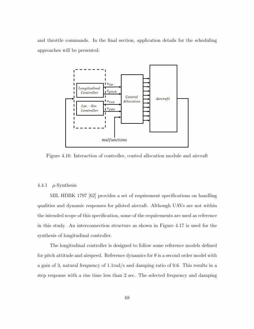
and throttle commands. In the final section, application details for the scheduling
approaches will be presented.
Figure 4.16: Interaction of controller, control allocation module and aircraft
4.4.1 µ-Synthesis
MIL HDBK 1797 [62] provides a set of requirement specifications on handling
qualities and dynamic responses for piloted aircraft. Although UAVs are not within
the intended scope of this specification, some of the requirements are used as reference
in this study. An interconnection structure as shown in Figure 4.17 is used for the
synthesis of longitudinal controller.
The longitudinal controller is designed to follow some reference models defined
for pitch attitude and airspeed. Reference dynamics for θ is a second order model with
a gain of 3, natural frequency of 1.1rad/s and damping ratio of 0.6. This results in a
step response with a rise time less than 2 sec. The selected frequency and damping
68

Figure 4.17: Longitudinal interconnection model for synthesis
values corresponds to Level I Flying Qualities, for gradual maneuvers of light aircraft
in MIL HDBK 1797.
Hmodelθ = 3(1.1)2
s2 + (2 ∗ 0.6 ∗ 1.1)s+ (1.1)2
Reference dynamics for airspeed is way slower, with about 10secs of rise time.
This is due to relatively slow engine dynamics and slow speed response of the air
vehicle. A gain of 9 is applied, meaning that unit input will result in an airspeed
change of 9 kts.
HmodelV = 9(0.3)2
s2 + (2 ∗ 1.0 ∗ 0.3)s+ (0.3)2
The Bode gain plots of the reference models is shown in Figure 4.18.
69

Figure 4.18: Bode gain plots for reference dynamicss
Sensor dynamics for pitch rate, pitch attitude and normal acceleration are im-
plemented as a combination of anti-aliasing filters and delays. The cutoff frequency
is assumed to be 4.1Hz for q and θ filters, and 12.5Hz for Nz filter. A delay of 20ms
is assumed for all sensors.
Hsensorq = Hsensorθ =(4.1 ∗ 2π)2
s2 + (2 ∗ 0.7 ∗ 4.1 ∗ 2π)s+ (4.1 ∗ 2π)2DPade
HsensorNz=
(12.5 ∗ 2π)2
s2 + (2 ∗ 0.5 ∗ 12.5 ∗ 2π)s+ (12.5 ∗ 2π)2DPade
2nd order Pade approximation for 20ms sensor delay is implemented.
DPade =s2 − 300s+ 30000
s2 + 300s+ 30000
70

Figure 4.19: Bode magnitude for anti-aliasing filters
Electro-mechanical servo actuators with 50rad/s cutoff and 0.7 damping is as-
sumed to be used for the flaps. As flaps are the primary effectors for pitching motion,
these values are used for the dynamic model of the virtual pitch command as well.
Hactpitch =(50)2
s2 + (2 ∗ 0.7 ∗ 50)s+ (50)2
Normally, actual throttle actuator dynamics is expected to be implemented
here for the virtual throttle model. However, as the linearized aircraft model does
not contain any states for engine dynamics, which is not fast enough to be totally
neglected, we insert engine dynamics into the synthesis model at this point. Since
throttle actuator dynamics is expected to be much faster than engine dynamics, it is
neglected. Therefore, the virtual throttle actuator model becomes:
Hactthr =(1.4)2
s2 + (2 ∗ 1.0 ∗ 1.4)s+ (1.4)2
71
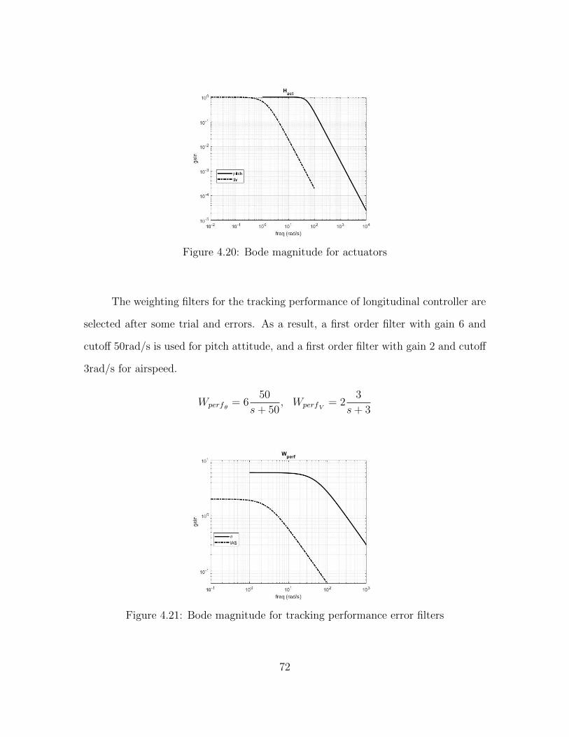
Figure 4.20: Bode magnitude for actuators
The weighting filters for the tracking performance of longitudinal controller are
selected after some trial and errors. As a result, a first order filter with gain 6 and
cutoff 50rad/s is used for pitch attitude, and a first order filter with gain 2 and cutoff
3rad/s for airspeed.
Wperfθ = 650
s+ 50, WperfV = 2
3
s+ 3
Figure 4.21: Bode magnitude for tracking performance error filters
72

Rate and attitude signals are assumed to be 2.5% noisy. Acceleration signals
are assumed to be pretty accurate for frequencies below 1rad/s and having a noise
ratio of 1.25% at high frequency.
Wnoise = diag(0.025,0.0125s+ 0.0125
s+ 100, 0.025)
Figure 4.22: Bode magnitude for Nz noise filter
Virtual pitch commands are allowed to change between -25◦ and +25◦ with a
rate up to 100◦/sec. Similarly virtual throttle command is assumed to change between
-25% and +25% with a rate up to 100%/sec. The maximum allowed rates may look
little bit too high at the first glance, however, they have been chosen so in order
to be able satisfy the robust performance requirements. Besides, the controllers are
observed to generate commands with much lower rates than the ones specified here.
Wact = diag(1
100,
1
50,
1
100,
1
50)
73

The multiplicative process uncertainty for pitch command is chosen to be about
1% below 1 rad/s and 100 % above 100 rad/s. As for the throttle command, uncer-
tainty is taken 0.1% below 0.01 rad/s and 100% above 10 rad/s.
Winppitch =s+ 1
s+ 100, Winpthr =
s+ 0.01
s+ 10
Figure 4.23: Bode magnitude for process uncertainty
An interconnection structure as shown in Figure 4.24 is used for the synthesis
of lateral-directional controller.
The lateral-directional controller is designed to follow some reference models
defined for roll attitude and sideslip. Reference dynamics for φ is a second order
model with a gain of 30, natural frequency of 0.7rad/s and damping ratio of 0.5. So,
maximum roll attitude with unit input is chosen to be 30◦, which is considered to be
quite sufficient for the intended missions of RQ-3. The military specification given in
Ref. [62], defines Level I performance as 60◦ bank in 1.7sec for light aircraft in gradual
maneuvers. The reference model gives 30◦ bank in 3.4sec. Although this value is much
74

Figure 4.24: Lateral-directional interconnection model for synthesis
slower than the specification, it is known that the intended use of the UAV is also
substantially different from the manned aircraft considered in the specification.
Hmodelφ = 30(0.7)2
s2 + (2 ∗ 0.5 ∗ 0.7)s+ (0.7)2
Although the primary role of the sideslip controller is to provide turn coordi-
nation, a tracker is also designed for flight conditions like approach in sidewind. The
controller provides a 5◦ slip to unit input with a rise time less than 2sec.
Hmodelβ = −5(1.25)2
s2 + (2 ∗ 1.0 ∗ 1.25)s+ (1.25)2
75

Figure 4.25: Bode magnitude for reference dynamics
Sensor dynamics for roll rate, yaw rate, roll attitude and lateral acceleration are
implemented as a combination of anti-aliasing filters and delays. The cutoff frequency
is assumed to be 4.1Hz for p and φ filters, and 12.5Hz for r and Ny filters. A delay
of 20ms is assumed for all sensors.
Hsensorp = Hsensorφ =(4.1 ∗ 2π)2
s2 + (2 ∗ 0.7 ∗ 4.1 ∗ 2π)s+ (4.1 ∗ 2π)2DPade
Hsensorr = HsensorNy=
(12.5 ∗ 2π)2
s2 + (2 ∗ 0.5 ∗ 12.5 ∗ 2π)s+ (12.5 ∗ 2π)2DPade
Figure 4.26: Bode magnitude for anti-aliasing filters
76

Flaps are the primary effectors for rolling motion as well, so the flap actuator
dynamics is also used for the virtual roll command. Spoilers are assumed to be driven
by slightly different actuators, with 50rad/s cutoff and 0.8 damping. Primary yaw
effectors are spoilers, so virtual yaw actuator dynamics is assumed to be same with
spoiler servo.
Hactroll =(50)2
s2 + (2 ∗ 0.7 ∗ 50)s+ (50)2
Hactyaw =(50)2
s2 + (2 ∗ 0.8 ∗ 50)s+ (50)2
Figure 4.27: Bode magnitude for roll and yaw virtual commands
A first order filter with gain 0.5 and cutoff 7rad/s is used for roll attitude, and
a first order filter with gain 2.5 and cutoff 10rad/s for sideslip.
Wperfφ = 0.57
s+ 7, Wperfβ = 2.5
10
s+ 10
77

Figure 4.28: Bode magnitude for tracking performance error filters
Rate and attitude signals are assumed to be 2.5% noisy. Acceleration signals
are assumed to be pretty accurate for frequencies below 1rad/s and having a noise
ratio of 1.25% at high frequency.
Wnoise = diag(0.025, 0.025,0.0125s+ 0.0125
s+ 100, 0.025)
Figure 4.29: Bode magnitude for noise
78

Both virtual roll and way commands are allowed to change between -25◦ and
+25◦ with a rate up to 100◦/sec.
Wact = diag(1
100,
1
50,
1
100,
1
50)
The multiplicative process uncertainty for roll command is chosen to be about
5% below 4 rad/s and 200% above 160 rad/s. For virtual yaw command, uncertainty
is taken 15% below 20 rad/s and 150% above 200 rad/s.
Winproll = 2s+ 4
s+ 160, Winpyaw = 1.5
s+ 20
s+ 200
Figure 4.30: Bode magnitude for process uncertainty
The controller synthesis is repeated for each operating point (or design point)
selected between 130-270 KIAS. As a consequence of the synthesis method selected,
each controller is an LTI system with an order much higher than the order of linear
aircraft model. The robust performance of the closed-loop system is guaranteed by
the synthesis method for the design points but this does not assure stability at any
flight conditions in between.
79

MATLAB-Robust Control Toolbox [63] is used as the synthesis tool. The fre-
quency band is selected between 10−2 rad/s and 102 rad/s. The maximum value of
the scaling matrix order is limited in order to obtain a similar controller order for
most of the design points. Also, in order to help the controller parameters be close
on neighboring design points, the initial controller used in D-K iteration is selected
as the controller synthesized in the previous design point.
Variation of closed-loop gain vs frequency at low, medium and high speed design
points are shown in Figure 4.31 for longitudinal closed-loop system and in Figure 4.32
for lateral directional closed-loop system. As can be followed from the figures, lateral-
directional system has much higher robustness margin compared to the longitudinal
one. The airspeed does not seem to have a considerable effect on the longitudinal
system, however, the robustness margin seems to increase with airspeed in the lateral-
directional.
4.4.2 Gain Scheduling
Ad-hoc Linear Interpolation:
A simple ad-hoc linear interpolation between the two controllers corresponding
to two consecutive design points is performed and the performance characteristics of
the resultant closed-loop system is investigated.
For two consecutive design points a, b where Pa, Pb are the bare (with no filters
etc.) linear plants and Ka, Kb are the controllers synthesized for the corresponding
interconnections, we define: P = Pa+Pb2
, ∆p = Pb−Pa2
and K = Ka+Kb2
, ∆k = Kb−Ka2
Following the approach explained in Chapter 2.5, the interpolated system can be
represented as the closed-loop system composed of plant P with an uncertainty ∆p
and controller K with an uncertainty ∆k as shown in Figure 4.33.
80

Figure 4.31: Performance of longitudinal controller
81

Figure 4.32: Performance of lateral-directional controller
82

Figure 4.33: Linearly interpolated system
µ-Analysis results obtained for the interpolated systems are shown in Fig-
ure 4.34. As can be followed, there is no significant change in the nominal performance
of the interpolated system, but the robust performance is deteriorated significantly.
Despite the loss in performance, the interpolated system is still stable and the inter-
polation will work fine for nominal system. However, this may not always be the case.
Especially when the two subsequent controllers differ significantly from each other,
the interpolation may end up with an unstable closed-loop system [64].
Synthesis using Simplified LPV Model:
A single controller for two consecutive design points can simply be synthesized
using linear Simplified LPV Model (Figure 2.15) as explained in Chapter 2.5. The
controller is assumed to be linear in parameters, and an interconnection shown in
Figure 2.16 is used. All components of the interconnection model are implemented as
defined in Chapter 4.4.1. The design points are the two LTI models linearized at 190
kts and 200 kts airspeeds. µ-Analysis results for the simplified LPV model synthesis
are shown in Figure 4.35.
A comparison of Figure 4.34 and Figure 4.35 reveals a difference between nom-
inal and robust (worst-case) performance between the linearly interpolated systems
and simplified LPV synthesis. The former has a low nominal gain, but very high
83

Figure 4.34: Performance for linearly interpolated systems
worst-case gain. However, for the latter, a far better worst case performance is evi-
dent with some sacrifice from the nominal performance.
Stability Preserving Interpolation:
The procedure applied for the implementation of Stability Preserving Inter-
polation is described in Table 4.7. All the steps in this procedure is based on the
formulation given in Chapter 2.5.
84

Table 4.7: Procedure for Stability Preserving Interpolation
Step Eqn.
1 (2.5),(2.6) For ρ ∈ [0, 1] and i = 1, 2Generate Linear State Space IC models for end points, Λ1, Λ2, Σ(0)and Σ(1)
2 (2.7) Calculate Fl(Σ(0),Λ2) and Fl(Σ(1),Λ1)3 From Σ(0) and Σ(1),
Extract F (0),G1(0),G2(0),H1(0) H2(0),J11(0),J12(0),J21(0),J22(0)Extract F (1),G1(1),G2(1),H1(1),H2(1),J11(1),J12(1),J21(1),J22(1)
4 (2.10) Extract A1(0) from Fl(Σ(0),Λ1)Extract A2(1) from Fl(Σ(1),Λ2)
5 Solve LMIs AT1 (0)W1(0) +W1(0)A1(0)< −I and W1(0)> 0 for W1(0)Solve LMIs AT2 (1)W2(1) +W2(1)A2(1)< −I and W2(1) > 0 for W2(1)
6 (2.23) Extract S1(0), N1(0), P1(0) from W1(0)Extract S2(1), N2(1), P2(1) from W2(1)Extract R1(0),M1(0), Q1(0) from W−1
1 (0)Extract R2(1),M2(1), Q2(1) from W−1
2 (1)7 (2.24) Calculate L1(0), L2(1), K1(0), K2(1)
8 (2.10) Calculate B1(0), C1(0), D1(0)Calculate B2(1), C2(1), D2(1)
9 (2.17) Select a value for interpolation parameter ρ′ where 0 ≤ ρ′ ≤ 1;Calculate W (ρ′), A(ρ′), B(ρ′), C(ρ′), D(ρ′)Calculate F (ρ′), G2(ρ′), H2(ρ′)
10 Calculate A1(ρ′), A2(ρ′)
11 Solve LMIs AT1 (ρ′)W1(ρ′)+W1(ρ′)A1(ρ′)< −I andW1(ρ′)> 0 forW1(ρ′)Solve LMIs AT2 (ρ′)W2(ρ′)+W2(ρ′)A2(ρ′)< −I and W2(ρ′)> 0 for W2(ρ′)
12 (2.23) Extract S1(ρ′), N1(ρ′) from W1(ρ′)Extract S2(ρ′), N2(ρ′) from W2(ρ′)Extract R1(ρ′),M1(ρ′) from W−1
1 (ρ′)Extract R2(ρ′),M2(ρ′) from W−1
2 (ρ′)13 (2.24) Calculate L1(ρ′), L2(ρ′), K1(ρ′), K2(ρ′)14 (2.26) Calculate S(ρ′), R(ρ′), L(ρ′), K(ρ′)15 (2.8) Calculate J (ρ′)16 Calculate Λ(ρ′) from Fl(J (ρ′),Q(ρ′))
85
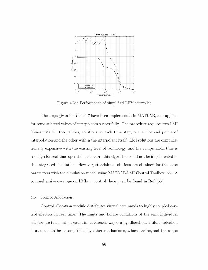
Figure 4.35: Performance of simplified LPV controller
The steps given in Table 4.7 have been implemented in MATLAB, and applied
for some selected values of interpolants successfully. The procedure requires two LMI
(Linear Matrix Inequalities) solutions at each time step, one at the end points of
interpolation and the other within the interpolant itself. LMI solutions are computa-
tionally expensive with the existing level of technology, and the computation time is
too high for real time operation, therefore this algorithm could not be implemented in
the integrated simulation. However, standalone solutions are obtained for the same
parameters with the simulation model using MATLAB-LMI Control Toolbox [65]. A
comprehensive coverage on LMIs in control theory can be found in Ref. [66].
4.5 Control Allocation
Control allocation module distributes virtual commands to highly coupled con-
trol effectors in real time. The limits and failure conditions of the each individual
effector are taken into account in an efficient way during allocation. Failure detection
is assumed to be accomplished by other mechanisms, which are beyond the scope
86

of this work, but failure isolation is a direct outcome of the implemented allocation
method.
All control allocation schemes need the B matrix, which is simply the rela-
tionship between virtual control commands and actual effector positions. In real
applications this relationship may not be linear or time invariant, however except for
the boundaries of the flight envelope, a fixed B is not a bad approximation. The B
matrix used in this study is given in Table 4.8. It is calculated at the neutral position
for each one of the effectors.
Table 4.8: B matrix used for control allocation
1 2 3 4 5
Left
∂CL/∂δi 4.8E-03 4.3E-03 3.6E-03 0.0E+00 0.0E+00∂CR/∂δi 3.7E-04 6.3E-04 8.4E-04 -1.8E-04 -2.4E-04∂CM/∂δi 1.8E-03 2.4E-03 4.2E-03 0.0E+00 0.0E+00∂CN/∂δi -1.6E-05 -2.4E-05 -2.9E-05 -1.4E-04 -2.4E-04
Right
∂CL/∂δi 4.8E-03 4.3E-03 3.6E-03 0.0E+00 0.0E+00∂CR/∂δi -3.7E-04 -6.3E-04 -8.4E-04 1.8E-04 2.4E-04∂CM/∂δi 1.8E-03 2.4E-03 4.2E-03 0.0E+00 0.0E+00∂CN/∂δi 1.6E-05 2.4E-05 2.9E-05 1.4E-04 2.4E-04
Modern aircraft use digital control systems which operate in discrete time. Con-
sidering the actuator position and rate constraints which are defined as:
δmin ≤ δ ≤ δmax,∣∣∣δ∣∣∣ ≤ δrate
Then, these can simply be merged for the sampling period T , such that [39]:
u ≤ u ≤ u
87

where
u(t) = max[δmin, u(t− T )− δrateT ] (4.21)
u(t) = min[δmax, u(t− T ) + δrateT ] (4.22)
Cascaded Generalized Inverse (CGI) [12][67]:
An algorithm using the CGI scheme has been implemented and tested in the
integrated simulation. The steps of this procedure is explained in Table 4.9.
Table 4.9: Procedure for Cascaded Generalized Inverse
Step
1 A single generalized inverse is used for calculating control effector com-mand, using (3.1).
2 If any control effector command is beyond saturation: ui < u or ui > u,then:
3 The saturated controls are left at limits, and removed from the problem.ui = u or ui = u
4 The columns of B associated with the saturated controls are removedto obtain B′
5 Total virtual commands vsat associated with the saturated controls uiis calculated:
vsat =nsat∑i=1
Biui
6 The saturated virtual command is removed from the original. υ =υ − υsat
7 The control allocation process is repeated with the reduced problem:B′u = υ
8 The process is repeated until υ is satisfied or no control effectors areleft to allocate.
Weighted Least Squares (WLS):
As a second approach, WLS formulation (3.2) for the control allocation problem
has been solved using an Active Set Algorithm [13][67]. Active set algorithm uses the
88
set of active constraints which is called Working Set-W . In each iteration step some
of the inequality constraints are regarded as equality constraints, and are included
in the working set, while the remaining inequality constraints are disregarded. The
working set at the optimum is known as the active set of the solution. For a generic
bounded least squares problem:
minu‖Au− b‖
with constraints;
Bu = υ, Cu ≥ U
considering our control allocation problem, C and U becomes:
C =
I
−I
, U =
u
−u
re-writing the cost function for WLS:
‖Wu(u− up)‖2 + γ‖Wυ(Bu− υ)‖2 =
∥∥∥∥∥∥∥ γWυB
Wu
u−
γWυv
Wuup
∥∥∥∥∥∥∥
2
the solution for u can be found by applying the procedure given in Table 4.10.
For more comprehensive information on the algorithms presented here, on dif-
ferent variants of these and on other control allocation algorithms as well, the reader
is suggested to refer Ref. [67].
4.6 Simulation Results
In this section the response of the integrated model, composed of the controller,
control allocation module and the nonlinear plant, to selected inputs will be studied
in detail. The performance of the implemented modules will be analyzed first for
the nominal case where no malfunction occurs, and then with different malfunction
89

Table 4.10: Procedure for Weighted Least Squares
Step
1 Let u0 be a feasible starting point and let the working set W containthe active inequality constraints at u0.
2 For each iteration k, for given uk, solve:
minp
∥∥A (uk + p)− b∥∥ , Bp = 0, pi = 0, i ∈ W
3a If uk+p is feasible, set uk+1=uk+p and compute the Lagrange multi-pliers, (µ, λ), where µ is associated with equality constraints, and λ isassociated with active inequality constraints.
3b If not, determine the maximum step length α such that uk+1 = uk +αpis feasible. Add the primary bounding constraint to the working set.
4a If all λ≥0 , uk+1 is the optimal solution, so exit the loop.4b If not remove the constraint associated with the most negative λ with
the working set.
scenarios. For all cases, a similar set of plots will be presented to make the comparison
easier. The parameters displayed on each plot is given in Table 4.11.
All simulations are performed in MATLAB-Simulink with fixed 10ms time step
using ODE5 Dormand-Prince integrator. The time history plots start five seconds
later than the simulation start, as the first few seconds are allocated for stabilization.
A single LTI controller model corresponding to the selected design point is used in
each run. No relative weighting is applied among control effectors.
Nominal Case:
The response of the aircraft to doublet shaped commands is investigated in this
part. The total simulation time is set to 100 sec. The airspeeds are selected as 150,
200, 250 KIAS corresponding to low, medium and high speed flight. In each run, the
doublets are applied in only single input channels, others left neutral. WLS method
is used for control allocation. The timing of the doublet is shown in Figure 4.36. Four
different maneuvers are executed as listed in Table 4.12.
90

Table 4.11: Parameters plotted
Symbol Unit Parameter
IAS kts Indicated airspeedθ, α deg Pitch attitude, Angle of attackφ deg Roll attitudeβ deg Angle of sideslip
p, q, r deg/s Body axis rotational rates for roll, pitch, yawNy, Nz g Body axis accelerations for lateral, vertical
υpitch, υroll, υyaw deg Virtual controller commands for pitch, roll, yawυthr pct Virtual controller command for throttle
δL1, δL2, δL3 deg Control effector angles for left flapsδR1, δR2, δR3 deg Control effector angles for right flapsδL4, δL5 deg Control effector angles for left spoilersδR4, δR5 deg Control effector angles for right spoilers
Figure 4.36: Doublet command
Table 4.12: Maneuver codes
No. Maneuver Amplitude
1 Pitch doublet 3◦
2 Roll doublet 30◦
3 IAS doublet 9 kts4 Sideslip doublet 3◦
Only mid speed results will be presented in the main body of this thesis and
other plots are going to be left for Appendix B.
91

200 KIAS - Pitch Doublet:
Time history plots for pitch doublet input are given in Figures 4.37 and 4.38.
Figure 4.37: Nominal, 200 KIAS, pitch doublet, plot 1
Figure 4.38: Nominal, 200 KIAS, pitch doublet, plot 2
92
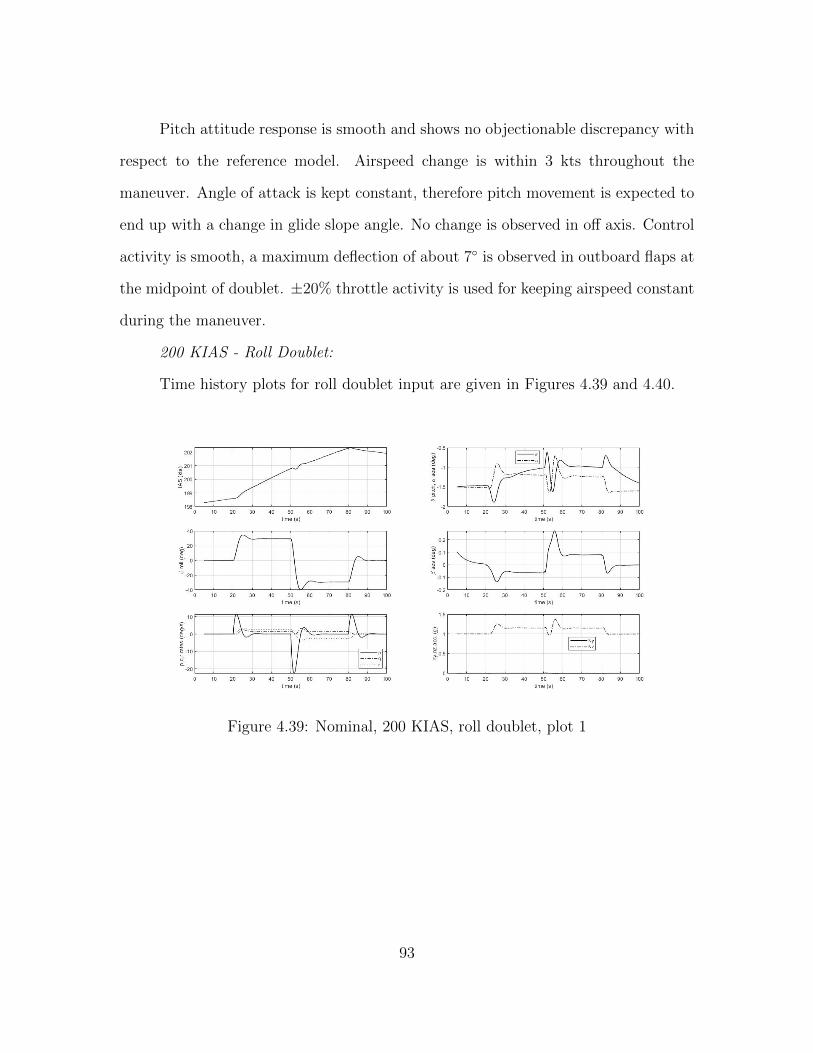
Pitch attitude response is smooth and shows no objectionable discrepancy with
respect to the reference model. Airspeed change is within 3 kts throughout the
maneuver. Angle of attack is kept constant, therefore pitch movement is expected to
end up with a change in glide slope angle. No change is observed in off axis. Control
activity is smooth, a maximum deflection of about 7◦ is observed in outboard flaps at
the midpoint of doublet. ±20% throttle activity is used for keeping airspeed constant
during the maneuver.
200 KIAS - Roll Doublet:
Time history plots for roll doublet input are given in Figures 4.39 and 4.40.
Figure 4.39: Nominal, 200 KIAS, roll doublet, plot 1
93

Figure 4.40: Nominal, 200 KIAS, roll doublet, plot 2
Roll attitude response is smooth and shows no objectionable discrepancy with
respect to the reference model. Angle of sideslip and lateral acceleration is kept close
to zero, so the turn is coordinated. Airspeed change is within 3 kts throughout the
maneuver. Change in pitch attitude and angle of attack is within 1◦ each. Control
activity is smooth, a maximum deflection of about 6◦ is observed in right outboard
flap at the midpoint of doublet. Spoiler deflections reaching up to 15◦ is observed.
Throttle activity is within 10% during the maneuver.
200 KIAS - Airspeed Doublet:
Time history plots for airspeed doublet input are given in Figures 4.41 and 4.42.
94
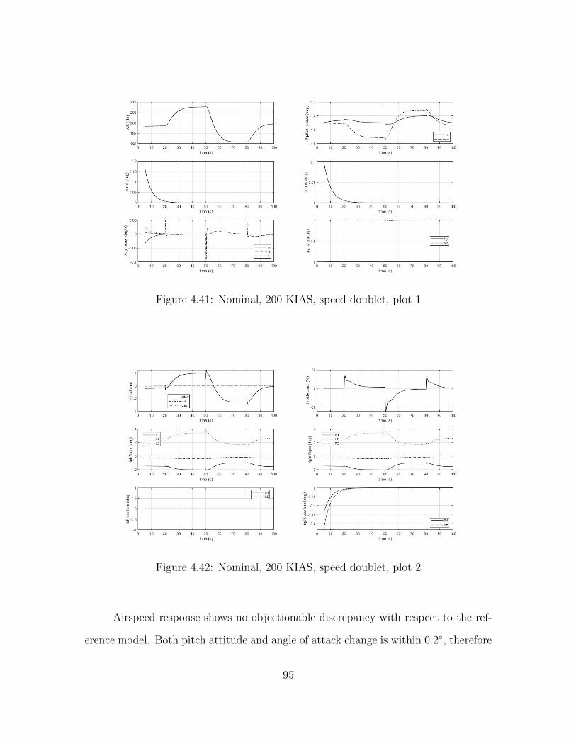
Figure 4.41: Nominal, 200 KIAS, speed doublet, plot 1
Figure 4.42: Nominal, 200 KIAS, speed doublet, plot 2
Airspeed response shows no objectionable discrepancy with respect to the ref-
erence model. Both pitch attitude and angle of attack change is within 0.2◦, therefore
95

no significant change in glide slope. No change is observed in off axis, as well. Control
activity is smooth, a maximum deflection of about 2◦ is observed in outboard flap.
+20%, -60% maximum throttle commands are observed.
200 KIAS - Sideslip Doublet:
Time history plots for sideslip doublet input are given in Figures 4.43 and 4.44.
Figure 4.43: Nominal, 200 KIAS, sideslip doublet, plot 1
96

Figure 4.44: Nominal, 200 KIAS, sideslip doublet, plot 2
Angle of sideslip response is smooth and shows no objectionable discrepancy
with respect to the reference model. A slight change in roll attitude is evident.
Airspeed change is close to 7-8 kts throughout the maneuver. Change in pitch attitude
and angle of attack is less than 0.6◦. Flap activity is quite limited. The sideslip is
generated by continuous deflection of spoilers by less than 15◦.
Now, the response of the simulation model to a series of step inputs will be
investigated. The main purpose is to compare the performance of the two control
allocation methods - CGI and WLS - in case of failed control effectors. In order
to generate a baseline, first no failure runs are performed for each of the control
allocation methods. All cases are run at 200 KIAS and the total simulation time is
set as 100 sec. The sequence of the step inputs in roll, pitch and sideslip is displayed
in Figure 4.45.
97

Figure 4.45: Sequence of step commands
CGI & WLS Baselines:
Time history plots for CGI and WLS baselines are given in Figures 4.46, 4.47
and Figures 4.48, 4.49.
Figure 4.46: CGI no failure baseline, plot 1
98

Figure 4.47: CGI no failure baseline, plot 2
Figure 4.48: WLS no failure baseline, plot 1
99

Figure 4.49: WLS no failure baseline, plot 2
A comparison of the Figure 4.46 with Figure 4.48 and Figure 4.47 with Fig-
ure 4.49 reveals no distinguishable difference. This means that, in nominal (no fail-
ure) case, the response and control activity using CGI and WLS control allocation
methods are similar. As the same controller is used in both cases and both control
allocation approaches tend to minimize control activity by keeping each effector angle
close to zero as possible, and no position or rate saturation or failure occurs during
the maneuver, two methods practically function similarly.
Malfunction Case:
The malfunctions applied in this simulation work are in two general types:
jamming and hard over. Jamming malfunctions are implemented by injecting a zero
rate limit in WLS allocation, and by injecting a fixed zero position in CGI allocation.
For hard over, a fixed maximum deflection is injected in both CGI and WLS. The
effected actuators are considered to be in their failure conditions throughout the
100
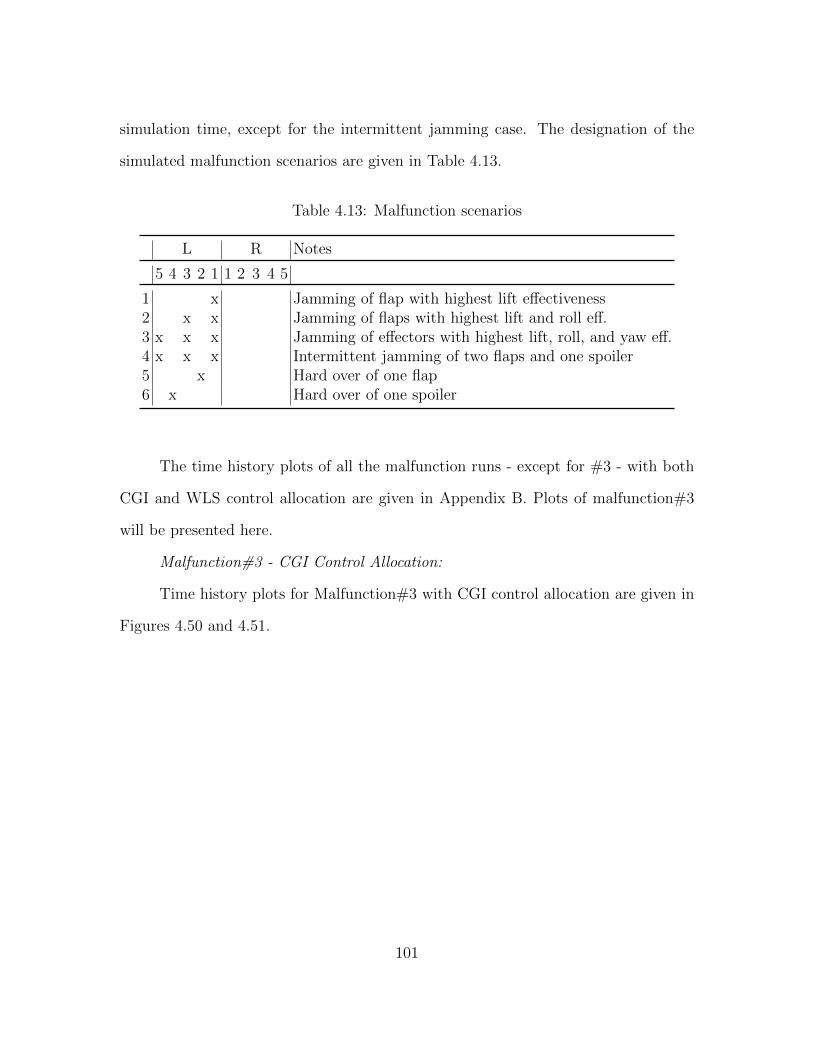
simulation time, except for the intermittent jamming case. The designation of the
simulated malfunction scenarios are given in Table 4.13.
Table 4.13: Malfunction scenarios
L R Notes
5 4 3 2 1 1 2 3 4 5
1 x Jamming of flap with highest lift effectiveness2 x x Jamming of flaps with highest lift and roll eff.3 x x x Jamming of effectors with highest lift, roll, and yaw eff.4 x x x Intermittent jamming of two flaps and one spoiler5 x Hard over of one flap6 x Hard over of one spoiler
The time history plots of all the malfunction runs - except for #3 - with both
CGI and WLS control allocation are given in Appendix B. Plots of malfunction#3
will be presented here.
Malfunction#3 - CGI Control Allocation:
Time history plots for Malfunction#3 with CGI control allocation are given in
Figures 4.50 and 4.51.
101

Figure 4.50: Malf#3, CGI control allocation, plot 1
Figure 4.51: Malf#3, CGI control allocation, plot 2
Left inboard flap, left outboard flap and left outboard spoiler is jammed at
neutral position. The malfunctions do not seem to cause a significant degradation in
102

system performance with CGI allocation. The system tracks the reference commands
in a smooth fashion without excessive use of remaining control effectors.
Malfunction#3 - WLS Control Allocation:
Time history plots for Malfunction#3 with WLS control allocation are given in
Figures 4.52 and 4.53.
Figure 4.52: Malf#3, WLS control allocation, plot 1
103

Figure 4.53: Malf#3, WLS control allocation, plot 2
The malfunctions do not seem to cause a significant degradation in system
performance with WLS allocation as well. Use of control effectors looks slightly
higher compared to CGI case.
None of the malfunction tests, even with the ones with three failed actuators,
resulted with significant degradation in tracking performance of reference commands.
However, in some of the tests, a small difference between the results of models using
CGI and WLS is observed. At the first glance, the tracking performance seems
smoother in CGI, and the effector usage is slightly less. But, when investigated
deeper, this difference is associated with the different convergence time of the two
control allocation modules in initialization phase. The control allocation modules
need a number of seconds to stabilize when a new simulation run starts. In most
scenarios, the malfunctions are effective from the very first instance of simulation.
Especially in multi-effector failure cases, the stabilization time becomes considerably
higher in WLS compared to CGI (Figure 4.54 and Figure 4.55) and so the system
104

initial states deviate more from trim. Time history plots of control effector angles in
the first five seconds of the simulation are given in Figures 4.54, 4.55, 4.56 and 4.57.
Figure 4.54: Effector angles, first 5 seconds, Malf#3 with CGI
105

Figure 4.55: Effector angles, first 5 seconds, Malf#3 with WLS
In cases where the malfunctions are injected later in the simulation, as in the
case of malfunction#4, the stabilization time is smaller (Figure 4.56 and Figure 4.57),
and consequently the performance of the two modules are close throughout the ma-
neuver.
106

Figure 4.56: Effector angles, first 5 seconds, Malf#4 with CGI
Figure 4.57: Effector angles, first 5 seconds, Malf#4 with WLS
107

Slower initial stabilization of WLS is considered to be related with its more
complicated structure and its dependence on the parameters calculated in the previous
time step, which imposes a small delay in the system.
Actuator position and rate limits can be merged (4.21) to form the effector
limits, which was discussed in Chapter 4.5. This is the approach followed in this
work for WLS allocation. However, as for CGI, this method did not perform well, so
only position limits could be implemented. In all the simulation work presented, CGI
allocation involves only position limits, whereas WLS involves both position and rate
limits.
In this part a comparison of CGI and WLS, when rate limits are implemented
in both is presented. An off-line simulation of two control allocation modules with a
given virtual command input is performed. In this example the rate limit for the left
outboard flap (L3) is set to 1◦/sec. An 80 sec part of time history plots for left flap
angles is presented in Figure 4.58.
108

Figure 4.58: CGI & WLS performance in case of limited rate
As can be followed, rate limited change of L3 around 150 sec and 200 sec is
evident for both CGI and WLS. In the same periods, a chatter occurs in L1 and L2
for CGI case. In WLS, limited rate in L3 does not seem to trigger any anomalies in
other effectors.
Uncertain Plant:
The performance of the control system in the case of plant uncertainties is
investigated in this part. Some aerodynamic parameters and servo transfer function
gains are assumed to be deviated from their nominal values as defined in the following.
The values of the deviation parameters are given in Table. 4.14.
(CD)unc = (CD)nom + ∆CD
109

(CL)unc = (CL)nom + kLCLαα + ∆CL
(CM)unc = (CM)nom + kMCMαα + ∆CM
(CYβ)unc = kY (CYβ)nom
(CNβ)unc = kN(CNβ)nom
(TFservo)unc = kservo(TFservo)nom
Table 4.14: Deviation from the nominal model
Parameter Deviation
∆CD +0.0050∆CL -0.02∆CM -0.02kL -10%kM -10%kY -5%kN -5%kservo -10%
A comparison for the tracking performance of the nominal plant with the deviated
plant is given in Figure 4.59, and a comparison of the virtual commands generated is
given in Figure 4.60.
110
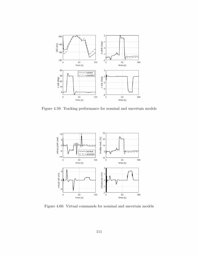
Figure 4.59: Tracking performance for nominal and uncertain models
Figure 4.60: Virtual commands for nominal and uncertain models
111

This single simulation shows that, even in a case of major deviation from the
anticipated model parameters, the system tracking performance is slightly effected.
However, for a thorough investigation, a Monte-Carlo analysis should be performed
by taking all the uncertainties into account.
112

CHAPTER 5
DISCUSSION
In this thesis, a study about the application of modern robust control design
techniques on a tailless UAV, RQ-3 Darkstar, is presented. First, a 6-DoF nonlinear
mathematical model for the vehicle is constructed using a semi empirical aerodynamic
prediction software: Digital DATCOM. A number of LTI plant models have been gen-
erated for selected operating points, based on this nonlinear model. Secondly, control
laws are synthesized for plant models generated at different operating points using
µ-synthesis design method. Three different approaches are investigated to schedule
the control laws: ad-hoc linear interpolation, synthesis using simplified LPV models
and stability preserving interpolation. Then, a control allocation module is imple-
mented to distribute the virtual commands, which are generated by the control laws,
to highly coupled control effectors in real time. Effector limits and failure conditions
are taken into account in an efficient way during allocation. Two different allocation
approaches are investigated: CGI and WLS. Finally, a simulation study is performed
using the nonlinear aircraft model, control laws and control allocation models for
various maneuvers and control effector failure cases.
Time history plots show that, for almost all maneuvers, the on-axis responses
are smooth and do not deviate from the reference model significantly. The only ex-
ception is a small beat in pitch virtual commands at the corners of the longitudinal
doublets. This is associated with a single small RHS zero apparent in the closed-loop
transfer function from pitch command. In the off-axis, a deviation in airspeed is
evident, especially for sideslip commands. This is considered to be related with the
113

coupling between longitudinal and lateral directional axes in 6-DoF equations of mo-
tion. Coupling problem can be solved by using cross feed terms between longitudinal
and lateral-directional controllers in more simple designs, but for our multivariable
method this is not applicable. A coupled synthesis using a full-state plant is con-
sidered as a reasonable solution for this problem. However, as the system order will
be much higher compared to decoupled case, the controller order and the level of
difficulty for implementation will be even higher, in this solution. This work can
be extended in the future by a full-state synthesis, taking aerodynamic and inertial
coupling terms into account.
Three interpolation methods are investigated for µ-synthesis. Ad-hoc linear
interpolation is simple from implementation point, but it gives no stability guarantees
for the interpolated systems. Even if the stability is preserved, robust performance
is shown to be much lower. Synthesis using simplified LPV models method is again
simple for implementation and gives much better robust performance, however, it is
applicable only between each two operating points and the problem of stitching all the
operating intervals still remains. Stability preserving interpolation is not simple but
straightforward for implementation, however it requires solution of LMIs at each time
step, which is considered not to be feasible with the available solvers. An extension to
this work can be done by investigating LFT synthesis based interpolation techniques,
in which a considerable amount of literature is available.
The malfunction simulations show no significant degradation in system perfor-
mance for the two allocation methods implemented. Even for cases with three failed
actuators, the system tracks the reference commands in a smooth fashion without
excessive use of remaining control effectors. WLS is observed to need a longer initial
stabilization period compared to CGI. However, this is considered to be a simulation
114
problem. In conditions where effector rate is limited, CGI is observed to result in a
small amplitude chatter, whereas, WLS is observed to perform well.
In this study, the controller is designed to create virtual commands in three
rotational axes: roll, pitch and yaw with no change in lift. However, for the flying
wing configuration, it is quite possible to create direct lift by using the effectors in a
proper sense. The structure of the control allocation module is designed compatible
for direct lift commands. A future study which makes use of this extra degree of
freedom is considered to be a very interesting extension to the current work.
The relationship between virtual control commands and actual effector posi-
tions, the B matrix, is assumed to be constant in control allocation algorithms, and
the uncertainty in it is associated with the process uncertainty in controller synthesis.
A method for implementing the change in B matrix can be studied as an extension
to the current work. As a result, the robustness of the system can be improved due
to the decrease in process uncertainty.
In µ-synthesis, further information about contributions of robust stability and
nominal performance requirements on the overall robust performance goal can be
extracted by decomposing closed-loop system matrix, M , into various constituents.
A systematic investigation of these contributions is considered to be an interesting
extension to the present work.
115

APPENDIX A
DATCOM INPUT CARDS
116

A.1 Datcom input card for symmetric flap
DIM M
DAMP
$FLTCON
STMACH=0.9, TSMACH=1.02,
NMACH=1.0, MACH(1)=0.4,
NALT=1.0, ALT=0.0,
NALPHA=20.0,
ALSCHD(1)=-8.0, -6.0, -4.0, -2.0, -1.0, 0.0, 1.0, 2.0, 4.0, 6.0, 8.0,
10.0, 12.0, 14.0, 15.0, 16.0, 17.0, 18.0, 19.0, 20.0,
LOOP=1.0$
$SYNTHS
XCG=2.965, ZCG=0.00,
XW=2.672, ZW=0.00, ALIW=1.00$
$BODY NX=9.0,
X(1)=0., 0.259, 0.958, 1.506, 2.157, 2.834, 3.539, 3.854, 4.247,
ZU(1)=0., 0.082, 0.437, 0.587, 0.651, 0.591, 0.385, 0.239, 0.0,
ZL(1)=0., -0.050, -0.168, -0.226, -0.246, -0.219, -0.138, -0.083, 0.0,
P(1)=0., 2.594, 4.932, 5.396, 5.488, 5.396, 5.116, 4.963, 0.0,
R(1)=0., 0.638, 1.143, 1.210, 1.210, 1.210, 1.210, 1.210, 0.0,
S(1)=0., 0.133, 1.086, 1.544, 1.704, 1.540, 0.994, 0.613, 0.0,
METHOD=1.0$
$WGPLNF CHRDTP=0.641, CHRDR=1.575, SSPN=10.515, SSPNE=9.075, SAVSI=-13.1,
DHDADI=0.0, TYPE=1.0$
$SYMFLP FTYPE=1.0, NDELTA=9.0,
117

DELTA(1)= -25., -20., -15., -5., 0., 5., 15., 20., 25.,
PHETE=0.117, CHRDFI=0.272, CHRDFO=0.227,
SPANFI=5.459, SPANFO=7.475$
$WGSCHR DWASH=1.0$
NACA-W-6-63-416
CASEID DARKSTAR 00100 SYMFLP - FLAP
NAMELIST
BUILD
NEXT CASE
A.2 Datcom input card for asymetric flap
DIM M
DAMP
$FLTCON
STMACH=0.9, TSMACH=1.02,
NMACH=1.0, MACH(1)=0.4,
NALT=1.0, ALT=0.0,
NALPHA=20.0,
ALSCHD(1)=-8.0, -6.0, -4.0, -2.0, -1.0, 0.0, 1.0, 2.0, 4.0, 6.0, 8.0,
10.0, 12.0, 14.0, 15.0, 16.0, 17.0, 18.0, 19.0, 20.0,
LOOP=1.0$
$SYNTHS
XCG=2.965, ZCG=0.00,
XW=2.672, ZW=0.00, ALIW=1.00$
118

$BODY NX=9.0,
X(1)=0., 0.259, 0.958, 1.506, 2.157, 2.834, 3.539, 3.854, 4.247,
ZU(1)=0., 0.082, 0.437, 0.587, 0.651, 0.591, 0.385, 0.239, 0.0,
ZL(1)=0., -0.050, -0.168, -0.226, -0.246, -0.219, -0.138, -0.083, 0.0,
P(1)=0., 2.594, 4.932, 5.396, 5.488, 5.396, 5.116, 4.963, 0.0,
R(1)=0., 0.638, 1.143, 1.210, 1.210, 1.210, 1.210, 1.210, 0.0,
S(1)=0., 0.133, 1.086, 1.544, 1.704, 1.540, 0.994, 0.613, 0.0,
METHOD=1.0$
$WGPLNF CHRDTP=0.641, CHRDR=1.575, SSPN=10.515, SSPNE=9.075, SAVSI=-13.1,
DHDADI=0.0, TYPE=1.0$
$ASYFLP STYPE=4.0, NDELTA=9.0,
DELTAL(1)= -25., -20., -15., -5., 0., 5., 15., 20., 25.,
DELTAR(1)= -0., -0., -0., -0., 0., 0., 0., 0., 0.,
PHETE=0.117, CHRDFI=0.272, CHRDFO=0.227,
SPANFI=5.459, SPANFO=7.475$
$WGSCHR DWASH=1.0$
NACA-W-6-63-416
CASEID DARKSTAR 00100 ASYMFLP - FLAP
NAMELIST
BUILD
NEXT CASE
A.3 Datcom input card for spoiler
DIM M
119

DAMP
$FLTCON
STMACH=0.9, TSMACH=1.02,
NMACH=1.0, MACH(1)=0.4,
NALT=1.0, ALT=0.0,
NALPHA=20.0,
ALSCHD(1)=-8.0, -6.0, -4.0, -2.0, -1.0, 0.0, 1.0, 2.0, 4.0, 6.0, 8.0,
10.0, 12.0, 14.0, 15.0, 16.0, 17.0, 18.0, 19.0, 20.0,
LOOP=1.0$
$SYNTHS
XCG=2.965, ZCG=0.00,
XW=2.672, ZW=0.00, ALIW=1.00$
$BODY NX=9.0,
X(1)=0., 0.259, 0.958, 1.506, 2.157, 2.834, 3.539, 3.854, 4.247,
ZU(1)=0., 0.082, 0.437, 0.587, 0.651, 0.591, 0.385, 0.239, 0.0,
ZL(1)=0., -0.050, -0.168, -0.226, -0.246, -0.219, -0.138, -0.083, 0.0,
P(1)=0., 2.594, 4.932, 5.396, 5.488, 5.396, 5.116, 4.963, 0.0,
R(1)=0., 0.638, 1.143, 1.210, 1.210, 1.210, 1.210, 1.210, 0.0,
S(1)=0., 0.133, 1.086, 1.544, 1.704, 1.540, 0.994, 0.613, 0.0,
METHOD=1.0$
$WGPLNF CHRDTP=0.641, CHRDR=1.575, SSPN=10.515, SSPNE=9.075, SAVSI=-13.1,
DHDADI=0.0, TYPE=1.0$
$ASYFLP STYPE=1.0, NDELTA=4.0,
DELTAS(1)= 0., 0.05, 0.1, 0.15,
XSOC(1)= 0.80, 0.75, 0.7, 0.65,
HSOC(1)= 0.07, 0.095, 0.12, 0.145,
120

PHETE=0.117, XSPRME=0.65,
SPANFI=8.988, SPANFO=10.500$
$WGSCHR DWASH=1.0$
NACA-W-6-63-416
CASEID DARKSTAR 00001 ASYFLP - SPOILER
NAMELIST
BUILD
NEXT CASE
121

APPENDIX B
SIMULATION - TIME HISTORY PLOTS
122

In this appendix, time history plots of the simulation results are presented.
Figure B.1: Nominal, 150 KIAS, pitch doublet, plot 1
Figure B.2: Nominal, 150 KIAS, pitch doublet, plot 2
123

Figure B.3: Nominal, 150 KIAS, roll doublet, plot 1
Figure B.4: Nominal, 150 KIAS, roll doublet, plot 2
124

Figure B.5: Nominal, 150 KIAS, speed doublet, plot 1
Figure B.6: Nominal, 150 KIAS, speed doublet, plot 2
125

Figure B.7: Nominal, 150 KIAS, sideslip doublet, plot 1
Figure B.8: Nominal, 150 KIAS, sideslip doublet, plot 2
126

Figure B.9: Nominal, 250 KIAS, pitch doublet, plot 1
Figure B.10: Nominal, 250 KIAS, pitch doublet, plot 2
127

Figure B.11: Nominal, 250 KIAS, roll doublet, plot 1
Figure B.12: Nominal, 250 KIAS, roll doublet, plot 2
128

Figure B.13: Nominal, 250 KIAS, speed doublet, plot 1
Figure B.14: Nominal, 250 KIAS, speed doublet, plot 2
129

Figure B.15: Nominal, 250 KIAS, sideslip doublet, plot 1
Figure B.16: Nominal, 250 KIAS, sideslip doublet, plot 2
130
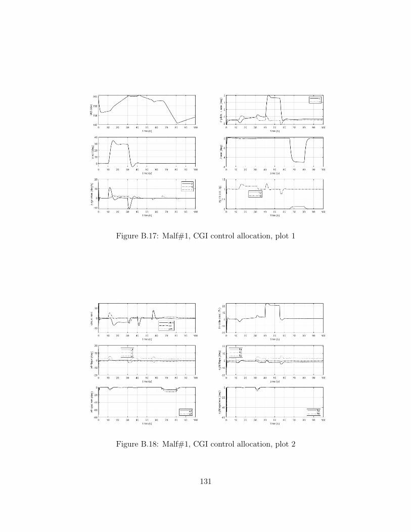
Figure B.17: Malf#1, CGI control allocation, plot 1
Figure B.18: Malf#1, CGI control allocation, plot 2
131

Figure B.19: Malf#1, WLS control allocation, plot 1
Figure B.20: Malf#1, WLS control allocation, plot 2
132

Figure B.21: Malf#2, CGI control allocation, plot 1
Figure B.22: Malf#2, CGI control allocation, plot 2
133
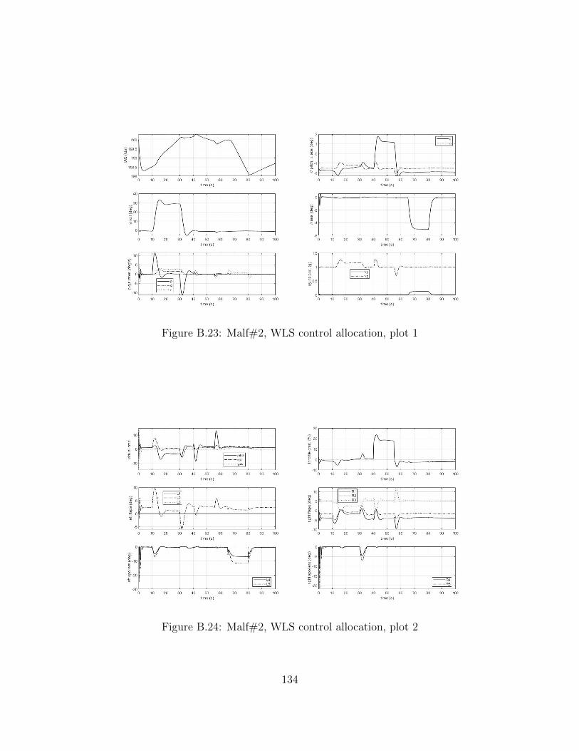
Figure B.23: Malf#2, WLS control allocation, plot 1
Figure B.24: Malf#2, WLS control allocation, plot 2
134

Figure B.25: Malf#4, CGI control allocation, plot 1
Figure B.26: Malf#4, CGI control allocation, plot 2
135

Figure B.27: Malf#4, WLS control allocation, plot 1
Figure B.28: Malf#4, WLS control allocation, plot 2
136
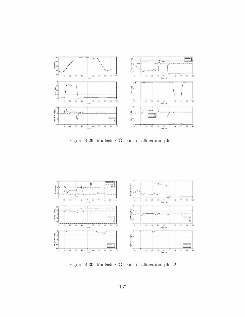
Figure B.29: Malf#5, CGI control allocation, plot 1
Figure B.30: Malf#5, CGI control allocation, plot 2
137

Figure B.31: Malf#5, WLS control allocation, plot 1
Figure B.32: Malf#5, WLS control allocation, plot 2
138

Figure B.33: Malf#6, CGI control allocation, plot 1
Figure B.34: Malf#6, CGI control allocation, plot 2
139

Figure B.35: Malf#6, WLS control allocation, plot 1
Figure B.36: Malf#6, WLS control allocation, plot 2
140

REFERENCES
[1] Colgren, R. and Loschke, R., “Effective Design of Highly Maneuverable Tailless
Aircraft,” AIAA Journal of Aircraft , Vol. 45, July 2008, pp. 1441 – 1449.
[2] Stenfelt, G. and Ringertz, U., “Lateral Stability and Control of a Tailless Aircraft
Configuration,” AIAA Journal of Aircraft , Vol. 46, Nov. 2009, pp. 2161 – 2164.
[3] Bolsunovsky, A., Buzoverya, N., Gurevich, B., Denisov, V., Dunaevsky, A.,
Shkadov, L., Sonin, O., Udzhuhu, A., and Zhurihin, J., “Flying Wing - Problems
and Decisions,” Aircraft Design, Vol. 4, Dec. 2001, pp. 193 – 219.
[4] Shtessel, Y., Buffington, J., and Banda, S., “Tailless Aircraft Flight Control
Using Multiple Time Scale Reconfigurable Sliding Modes,” IEEE Transactions
on Control Systems Technology , Vol. 10, March 2002, pp. 288 – 296.
[5] Gundlach, J., Designing Unmanned Aircraft Systems: A Comprehensive Ap-
proach, AIAA Education Series, Reston, VA, 2012.
[6] Castro, H. D., Flying and Handling Qualities of a Fly-by-Wire Blended Wing
Body Civil Transport Aircraft , Ph.D. thesis, Cranfield University, Cranfield, UK,
2003.
[7] Seckel, E., Stability and Control of Aircraft and Helicopters , Academic Press,
New York, NY, 1964.
[8] “The USAF Stability and Control Digital DATCOM, Volume I, Users Man-
ual,” Tech. Rep. AFFDL-TR-79-3032, McDonnell Douglas Astronautics Com-
pany, St.Louis, MO, 1979.
[9] “Application of Multivariable Control Theory to Aircraft Control Laws, Final
Report: Multivariable Control Design Guidelines,” Tech. Rep. WL-TR-96-3099,
141
Honeywell Technology Center, Lockheed Martin Skunk Works, Lockheed Martin
Tactical Aircraft Systems, 1996.
[10] Natesan, K., Da-Wei, G., Postlethwaite, I., and Jianchi, C., “Design of Flight
Controllers based on Simplified LPV model of a UAV,” Proceedings of the 45th
IEEE Conference on Decision and Control , Dec. 2006.
[11] Stilwell, D. J. and Rugh, W. J., “Stability Preserving Interpolation Methods for
the Synthesis of Gain Scheduled Controllers,” Automatica, Vol. 36, 2000, pp. 665
– 671.
[12] Durham, W., Bordignon, K., and Beck, R., Aircraft Control Allocation, John
Wiley & Sons, Chickester, West Sussex, UK, 2017.
[13] Harkegard, O., “Efficient Active Set Algorithms for Solving Constrained Least
Squares Problems in Aircraft Control Allocation,” Proceedings of the 41st IEEE
Conference on Decision and Control , 2002.
[14] Skogestad, S. and Postlethwaite, I., Multivariable Feedback Control Analysis and
Design, John Wiley & Sons, Chickester, West Sussex, UK, 2005.
[15] Stevens, B., Lewis, F., and Johnson, E., Aircraft Control and Simulation - Third
ed., Wiley, Hoboken, NJ, 2016.
[16] Amato, F. and Iervolino, R., “µ-Synthesis for a Small Commercial Aircraft:
Design and Simulator Validation,” AIAA Journal of Guidance, Control, and
Dynamics , Vol. 27, May 2004, pp. 479 – 490.
[17] Hyde, R. A. and Glover, K., “The Application of Scheduled H∞ Controllers to a
VSTOL Aircraft,” IEEE Transactions on Automatic Control , Vol. 38, July 1993,
pp. 1021.
[18] Aouf, N. and Boulet, B., “Linear Fractional Transformation Gain-Scheduling
Flight Control Preserving Robust Performance,” Journal of Aerospace Engineer-
ing , Vol. 226, July 2012, pp. 763 – 773.
142

[19] Natesan, K., Gu, D., and Postlethwaite, I., “Design of Linear Parameter Vary-
ing Trajectory Tracking Controllers for an Unmanned Air Vehicle,” Journal of
Aerospace Engineering , Vol. 224, April 2010, pp. 395 – 402.
[20] Mystkowski, A., “An Application of µ-Synthesis to Control of a Small Air Vehicle
and Simulation Results,” Journal of Vibroengineering , Vol. 14, March 2012.
[21] Nichols, R., Reichert, R., and Rugh, W., “Gain Scheduling for H∞ Controllers:
A Flight Control Example,” IEEE Transactions on Control Systems Technology ,
Vol. 1, June 1993, pp. 69 – 79.
[22] Biannic, J.-M., Apkarian, P., and Garrard, W. L., “Parameter Varying Control
of a High Performance Aircraft,” Journal of Guidance, Control, and Dynamics ,
Vol. 20, March 1997, pp. 225 – 231.
[23] Turkoglu, E., Application of Robust Control to a Rotary-Wing Aircraft , Ph.D.
thesis, University of Leicester, Leicester, UK, 2007.
[24] Greenberg, M., Advanced Engineering Mathematics - 2nd Edition, Prentice Hall,
Upper Saddle River, NJ, 1998.
[25] Ogata, K., Modern Control Engineering - 5th Edition, Prentice Hall, Upper
Saddle River, NJ, 2010.
[26] Frazzoli, E., “MIT Open Courseware, Lecture Notes,” Internet draft, 2004.
[27] Balas, G., Doyle, J., Glover, K., Packard, A., and Smith, R., µ-Analysis and
Synthesis Toolbox - Users Guide - Version 3 , The Mathworks Inc., Natick, MA,
2001.
[28] Nalbantoglu, V., Robust Control and System Identification for Flexible Struc-
tures , Ph.D. thesis, University of Minnesota, MN, 1998.
[29] Zhou, K., Doyle, J., and Glover, K., Robust and Optimal Control , Prentice Hall,
Englewood Cliffs, NJ, 1995.
143

[30] Shamma, J. S. and Cloutier, J. R., “Gain-Scheduled Missile Autopilot Design Us-
ing Linear Parameter Varying Transformations,” Journal of Guidance, Control,
and Dynamics , Vol. 16, 1993, pp. 256 – 263.
[31] Biannic, J.-M. and Apkarian, P., “Missile Autopilot Design via a Modified LPV
Synthesis Technique,” Aerospace Science and Technology , Vol. 3, 1999, pp. 153
– 160.
[32] Marcos, A. and Balas, G. J., “Development of Linear-Parameter-Varying Models
for Aircraft,” Journal of Guidance, Control, and Dynamics , Vol. 27, March 2004,
pp. 218 – 228.
[33] Packard, A., “Gain scheduling via Linear Fractional Transformations,” Systems
& Control Letters , Vol. 22, 1994, pp. 79 – 92.
[34] Helmersson, A., “µ-Synthesis and LFT Gain Scheduling with Mixed Uncertain-
ties,” International Journal of Robust and Nonlinear Control , Vol. 8, June 1998,
pp. 631 – 642.
[35] Magni, J., “An LFT Approach to Robust Gain Scheduling,” Proceedings of the
44th IEEE Conference on Decision and Control , 2005.
[36] Natesan, K., Da-Wei, G., Postlethwaite, I., and Jianchi, C., “Design of Flight
Controllers based on Simplified LPV model of a UAV,” Proceedings of the 45th
IEEE Conference on Decision and Control , Dec. 2006.
[37] Stilwell, D. J., “State Space Interpolation for a Gain-Scheduled Autopilot,” Jour-
nal of Guidance, Control, and Dynamics , Vol. 24, May 2001, pp. 460 – 465.
[38] Johansen, T. A. and Fossen, T. I., “Control Allocation - A Survey,” Automatica,
Vol. 49, May 2013, pp. 1087 – 1103.
[39] Harkegaard, O., “Dynamic Control Allocation Using Constrained Quadratic Pro-
gramming,” Journal of Guidance, Control, and Dynamics , Vol. 27, Nov. 2004,
pp. 1028 – 1034.
144

[40] Enns, D., “Control Allocation Approaches,” 1998.
[41] Nieto-Wire, C., Eigenstructure Assignement for a Tailless Aircraft , Ph.D. thesis,
The City University of New York, NY, 2012.
[42] Wise, K. A., Brinker, J. S., Calise, A. J., Enns, D. F., Elgersma, M. R., and Voul-
garis, P., “Direct Adaptive Reconfigurable Flight Control for a Tailless Advanced
Fighter Aircraft,” International Journal of Robust and Nonlinear Control , Vol. 9,
Dec. 1999, pp. 999 – 1012.
[43] Chen, S., Adaptive Control of Nonlinear Systems with Actuator Failures and
Uncertainities , Ph.D. thesis, University of Virginia, VA, 2004.
[44] Naskar, A. K., Patra, S., and Sen, S., “A Reconfigurable Direct Control Alloca-
tion Method,” 2013 European Control Conference (ECC), July 2013.
[45] Kroo, I., “Tailless Aircraft Design - Recent Experiences,” Proceedings of the
Symposium on Aerodynamics and Aeroacoustics , Tucson, AZ.
[46] Nickel, K. and Wohlfahrt, M., Tailless Aircraft in Theory and Practice, Butter-
worth - Heinemann, Burlington, MA, 2003.
[47] Peterson, T., Handling Qualities of a Blended Wing Body Aircraft , Master’s
thesis, University of Toronto, Canada, 2011.
[48] Kroo, I., Aerodynamics, Aeroelasticity and Stability of Hang Gliders , Ph.D. the-
sis, Stanford University, CA, 1983.
[49] Cusher, A. A. and Gopalarathnam, A., “Drag Reduction Methodology for Adap-
tive Tailless Aircraft,” Journal of Aircraft , Vol. 49, Jan. 2012, pp. 161 – 172.
[50] Ashkenas, I. and Clyde, D., “Tailless Aircraft Performance Improvements with
Relaxed Static Stability,” Tech. Rep. NASA CR-181806, Systems Technology,
Inc., Hawthorne, CA, 1989.
[51] Calise, A., Lee, S., and Sharma, M., “Direct Adaptive Reconfigurable Control of
a Tailless Fighter Aircraft,” 1998.
145

[52] Peterson, T., On the use of Active Flow Control to Trim and Control a Tailless
Aircraft Model , Master’s thesis, The University of Arizona, Tucson, AZ, 2017.
[53] Saephan, S., Determination of Tailless Aircraft Tumbling and Stability Char-
acteristics Through Computational Fluid Dynamics , Ph.D. thesis, University of
California, Davis, CA, 2006.
[54] Park, J., Choi, J.-Y., Jo, Y., and Choi, S., “Stability and Control of Tailless
Aircraft Using Variable Fidelity Aerodynamic Analysis,” Journal of Aircraft ,
Vol. 54, Nov. 2017, pp. 2148 – 2164.
[55] Stenfelt, G., Aerodynamics and Lateral Control of Tailless Aircraft , Ph.D. thesis,
Royal Institute of Technology, Stockholm, Sweden, 2011.
[56] “RQ-3 Darkstar,” 2019.
[57] Cavalcanti, S. and Papini, M., “Preliminary Model Matching of the EMBRAER
170 Jet,” Journal of Aircraft , Vol. 41, July 2004, pp. 703 – 710.
[58] Watters, B., Adaptation of Digital Datcom into a Conceptual Design Process ,
Master’s thesis, The University of Texas at Arlington, TX, 2011.
[59] “USAF Stability and Control Datcom,” Tech. rep., McDonnell Douglas Corpo-
ration, 1978.
[60] Botez, R. M., Bardela, P. A., and Bournisien, T., “Cessna Citation X Simulation
Turbofan Modelling: Identification and Identified Model Validation using Sim-
ulated Flight Tests,” The Aeronautical Journal , Vol. 123, April 2019, pp. 433 –
463.
[61] Dreier, M. E., Introduction to Helicopter and Tiltrotor Simulation, AIAA Edu-
cation Series, Reston, VA, 2007.
[62] “Flying Qualities of Piloted Aircraft,” Tech. Rep. MIL HDBK 1797, U.S. De-
partment of Defense, 1997.
146
[63] Balas, G., Chiang, R., Packard, A., and Safonov, M., Robust Control Toolbox -
User’s Guide, The Mathworks Inc., Natick, MA, 2019.
[64] Shamma, J. and Athans, M., “Gain Scheduling: Potential Hazards and Possible
Remedies,” IEEE Control Systems , Vol. 12, June 1992, pp. 101 – 107.
[65] Gahinet, P., Nemirovski, A., Laub, A., and Chilali, M., LMI Control Toolbox -
User’s Guide, The Mathworks Inc., Natick, MA, 1995.
[66] Boyd, S., Ghaoui, L. E., Feron, E., and Balakrishnan, V., Linear Matrix Inequal-
ities in System and Control Theory , SIAM, Philadelphia, PA, 1994.
[67] Harkegaard, O., “QCAT Documentation,” 2019.
147


![Autonomous Navigation of UAV in Foliage Environmentbmchen/papers/JIRS-2016-02.pdf · design a Robust and Perfect Tracking (RPT) control law [16] to control the UAV outer loop to track](https://img.dokumen.tips/doc/110x75/5d06449688c993dd5e8d7fa5/autonomous-navigation-of-uav-in-foliage-bmchenpapersjirs-2016-02pdf-design.jpg)