CA NGSS Roll Out #3: Learning Sequence Example, Grades 6-8

1

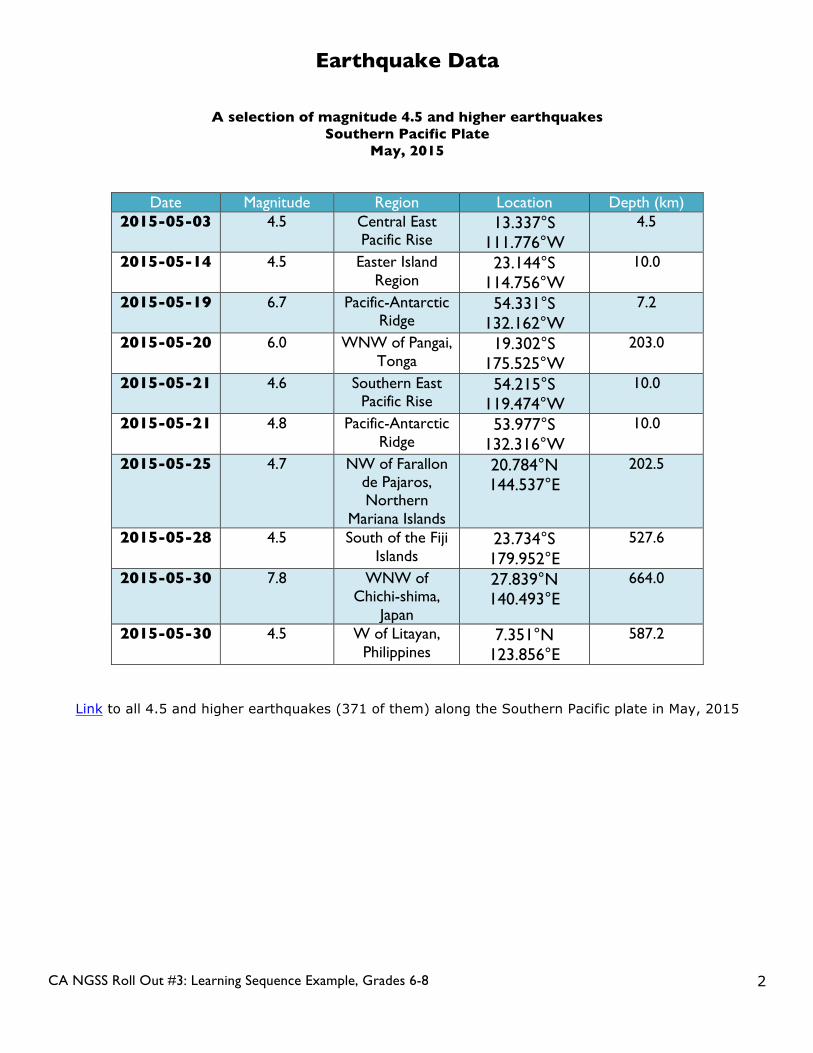
A Revolution Revival: Seismology During the 20th century, worldwide improvements in technology used to study seismic events and greater use of earthquake-recording instruments (seismographs) enabled scientists to discover some interesting patterns! For the first time ever, better data from the Worldwide Standardized Seismograph Network in the 1960’s allowed scientists to map earthquakes worldwide in a very accurate way.

What pattern did scientists notice?

Use your Simplified Plate Tectonic Map handout and use a small shape to mark the location of the earthquakes from the earthquake data handout given to you. As you mark, color code the earthquakes by depth:

Orange: Shallow earthquakes are between 0 and 70 km deep Green: intermediate earthquakes, 70 - 300 km deep Blue: deep earthquakes, 300 - 700 km deep.

Discuss what pattern(s) your group notices and be ready to report back to your team.

Help box

In order to mark your map, you must understand the concepts of latitude and longitude. All lines of latitude run parallel to the equator. There are 90° of latitude to the north and 90° of latitude to the south of the equator. Degrees to the north are labeled as positive, while degrees to the south are labeled as negative. Each degree of latitude is approximately 111 km apart.

Source: http://www.dpc.ucar.edu/projects/revEdSite/lp3_subd_zone.html Narrative adapted from http://pubs.usgs.gov/gip/dynamic/developing.html Emoji from http://emojipedia.org/smiling-face-with-sunglasses/

H12b

CA NGSS Roll Out #3: Learning Sequence Example, Grades 6-8

2

Earthquake Data

A selection of magnitude 4.5 and higher earthquakes Southern Pacific Plate

May, 2015

Date Magnitude Region Location Depth (km) 2015-05-03 4.5 Central East

Pacific Rise 13.337°S

111.776°W 4.5

2015-05-14 4.5 Easter Island Region

23.144°S 114.756°W

10.0

2015-05-19 6.7 Pacific-Antarctic Ridge

54.331°S 132.162°W

7.2

2015-05-20 6.0 WNW of Pangai, Tonga

19.302°S 175.525°W

203.0

2015-05-21 4.6 Southern East Pacific Rise

54.215°S 119.474°W

10.0

2015-05-21 4.8 Pacific-Antarctic Ridge

53.977°S 132.316°W

10.0

2015-05-25 4.7 NW of Farallon de Pajaros, Northern

Mariana Islands

20.784°N 144.537°E

202.5

2015-05-28 4.5 South of the Fiji Islands

23.734°S 179.952°E

527.6

2015-05-30 7.8 WNW of Chichi-shima,

Japan

27.839°N 140.493°E

664.0

2015-05-30 4.5 W of Litayan, Philippines

7.351°N 123.856°E

587.2

Link to all 4.5 and higher earthquakes (371 of them) along the Southern Pacific plate in May, 2015

CA NGSS Roll Out #3: Learning Sequence Example, Grades 6-8

3

This Dynamic Planet; A Teaching CompanionPlate Tectonics Tennis Ball GlobeU.S. Geological Survey, 2008 revised from This Dynamic Planet MapFor updates see <http://volcanoes.usgs.gov/about/edu/dynamicplanet>

U.S. Department of the InteriorU.S. Geological Survey

GUS SSimplified Plate Tectonics Map

Plate boundary - Known area between two plates.

Some plate boundaries, such as the North America - South America boundary, are not shown because scientific dataare inadequate to determine precise locations. See the This Dynamic Planet Map insert for more information about these regions.

H13

CA NGSS Roll Out #3: Learning Sequence Example, Grades 6-8

4

H14a

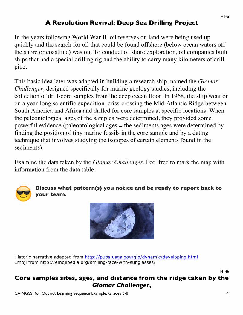
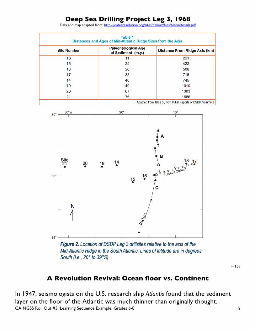
A Revolution Revival: Deep Sea Drilling Project In the years following World War II, oil reserves on land were being used up quickly and the search for oil that could be found offshore (below ocean waters off the shore or coastline) was on. To conduct offshore exploration, oil companies built ships that had a special drilling rig and the ability to carry many kilometers of drill pipe. This basic idea later was adapted in building a research ship, named the Glomar Challenger, designed specifically for marine geology studies, including the collection of drill-core samples from the deep ocean floor. In 1968, the ship went on on a year-long scientific expedition, criss-crossing the Mid-Atlantic Ridge between South America and Africa and drilled for core samples at specific locations. When the paleontological ages of the samples were determined, they provided some powerful evidence (paleontological ages = the sediments ages were determined by finding the position of tiny marine fossils in the core sample and by a dating technique that involves studying the isotopes of certain elements found in the sediments). Examine the data taken by the Glomar Challenger. Feel free to mark the map with information from the data table.

Discuss what pattern(s) you notice and be ready to report back to your team.

Historic narrative adapted from http://pubs.usgs.gov/gip/dynamic/developing.html Emoji from http://emojipedia.org/smiling-face-with-sunglasses/

H14b

Core samples sites, ages, and distance from the ridge taken by the Glomar Challenger,

CA NGSS Roll Out #3: Learning Sequence Example, Grades 6-8

5

Deep Sea Drilling Project Leg 3, 1968 Data and map adapted from: http://joidesresolution.org/sites/default/files/Nannofossils.pdf

H15a

A Revolution Revival: Ocean floor vs. Continent

In 1947, seismologists on the U.S. research ship Atlantis found that the sediment layer on the floor of the Atlantic was much thinner than originally thought.

CA NGSS Roll Out #3: Learning Sequence Example, Grades 6-8

6

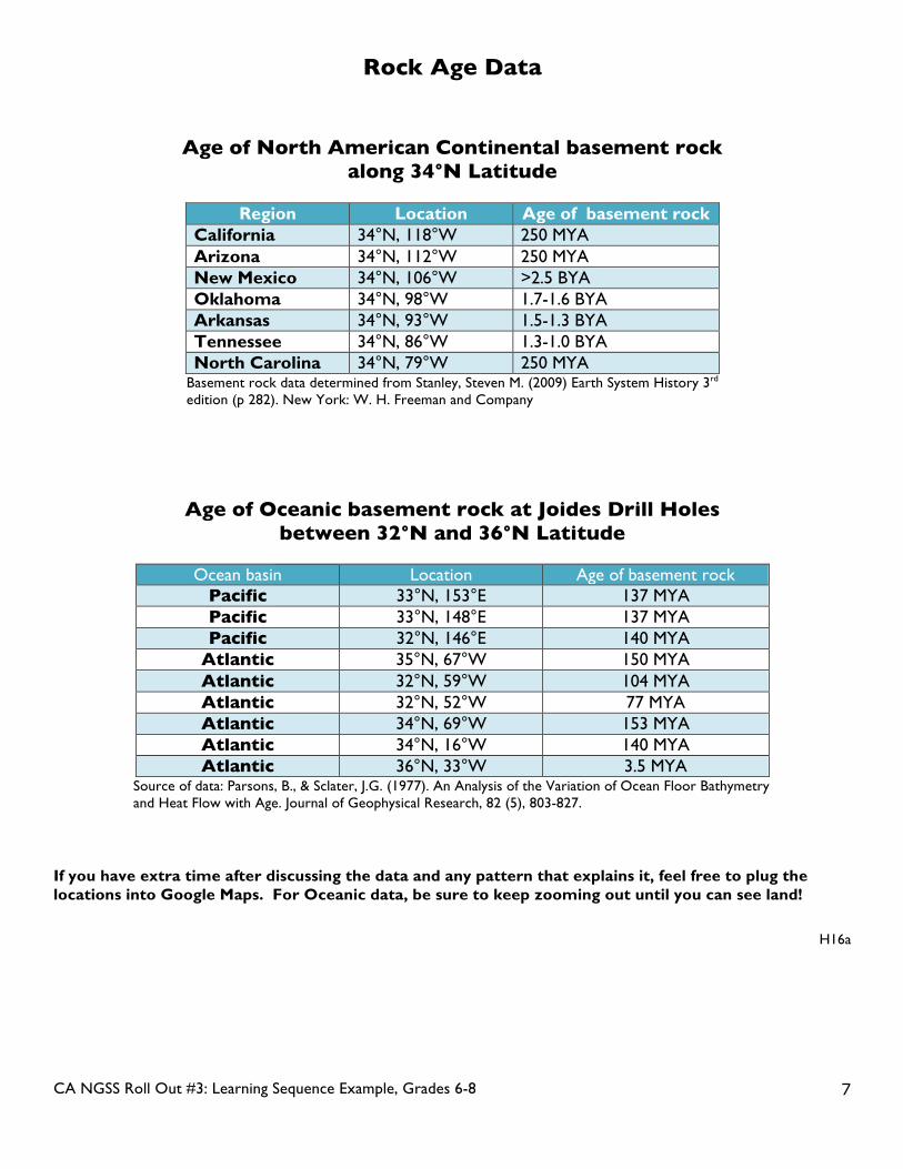
Scientists had previously believed that the oceans have existed for at least 4 billion years, so they had assumed the sediment layer should have been very thick. They were surprised to find so little accumulation of sedimentary rock and debris on the ocean floor and wondered how this could be possible. Meanwhile, an international partnership of scientists and governments joined together to create the Ocean Drilling Program, allowing scientists a unique opportunity to get samples of ocean floor rock. They expected to find rock ages similar to what we find on continental rock, but when they determined the ages of the oceanic rocks many were surprised! Here we provide you with some rock age data that will include continental basement rock (igneous and metamorphic rock found on continents that is the foundation of the continent below sediments) and ocean floor rock.

Key MYA = Millions of years ago BYA = Billions of years ago

Joides = Scientific drilling ship

Discuss what pattern(s) you notice and be ready to report back to your team.

Historic narrative adapted from http://pubs.usgs.gov/gip/dynamic/developing.html and http://www.odplegacy.org/PDF/Data/Documentation/ODP_Data.pdf Emoji from http://emojipedia.org/smiling-face-with-sunglasses/

H15b

CA NGSS Roll Out #3: Learning Sequence Example, Grades 6-8

7

Rock Age Data

Age of North American Continental basement rock along 34°N Latitude

Region Location Age of basement rock

California 34°N, 118°W 250 MYA Arizona 34°N, 112°W 250 MYA New Mexico 34°N, 106°W >2.5 BYA Oklahoma 34°N, 98°W 1.7-1.6 BYA Arkansas 34°N, 93°W 1.5-1.3 BYA Tennessee 34°N, 86°W 1.3-1.0 BYA North Carolina 34°N, 79°W 250 MYA

Basement rock data determined from Stanley, Steven M. (2009) Earth System History 3rd edition (p 282). New York: W. H. Freeman and Company

Age of Oceanic basement rock at Joides Drill Holes between 32°N and 36°N Latitude

Ocean basin Location Age of basement rock

Pacific 33°N, 153°E 137 MYA Pacific 33°N, 148°E 137 MYA Pacific 32°N, 146°E 140 MYA

Atlantic 35°N, 67°W 150 MYA Atlantic 32°N, 59°W 104 MYA Atlantic 32°N, 52°W 77 MYA Atlantic 34°N, 69°W 153 MYA Atlantic 34°N, 16°W 140 MYA Atlantic 36°N, 33°W 3.5 MYA

Source of data: Parsons, B., & Sclater, J.G. (1977). An Analysis of the Variation of Ocean Floor Bathymetry and Heat Flow with Age. Journal of Geophysical Research, 82 (5), 803-827.

If you have extra time after discussing the data and any pattern that explains it, feel free to plug the locations into Google Maps. For Oceanic data, be sure to keep zooming out until you can see land!

H16a

CA NGSS Roll Out #3: Learning Sequence Example, Grades 6-8

8

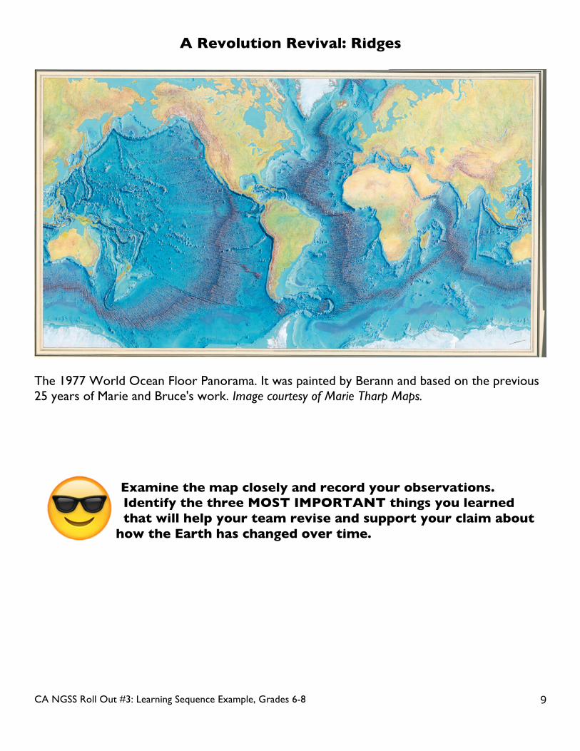
A Revolution Revival: Ridges

"Modern" measurements of ocean depths greatly increased in the 19th century, when deep-sea line soundings (bathymetric surveys) were routinely made in the Atlantic and Caribbean. Basically, this involved lowering down a line with a weight (sounding lead) to the bottom of the ocean, and measuring the length of the line.

Simplified maps, called bathymetric chart published by U.S. Navy Lieutenant Matthew Maury revealed the first evidence of underwater mountains in the central Atlantic (which he called "Middle Ground"). This was later confirmed by survey ships laying the trans-Atlantic telegraph cable. Our picture of the ocean floor greatly sharpened after World War I (1914-18), when echo-sounding devices -- primitive sonar systems -- began to measure ocean depth by recording the time it took for a sound signal (commonly an electrically generated "ping") from the ship to bounce off the ocean floor and return. Time graphs of the returned signals revealed that the ocean floor was much more rugged than previously thought. Such echo-sounding measurements clearly demonstrated the continuity and roughness of the submarine mountain chain in the central Atlantic (later called the Mid-Atlantic Ridge) suggested by the earlier bathymetric measurements.

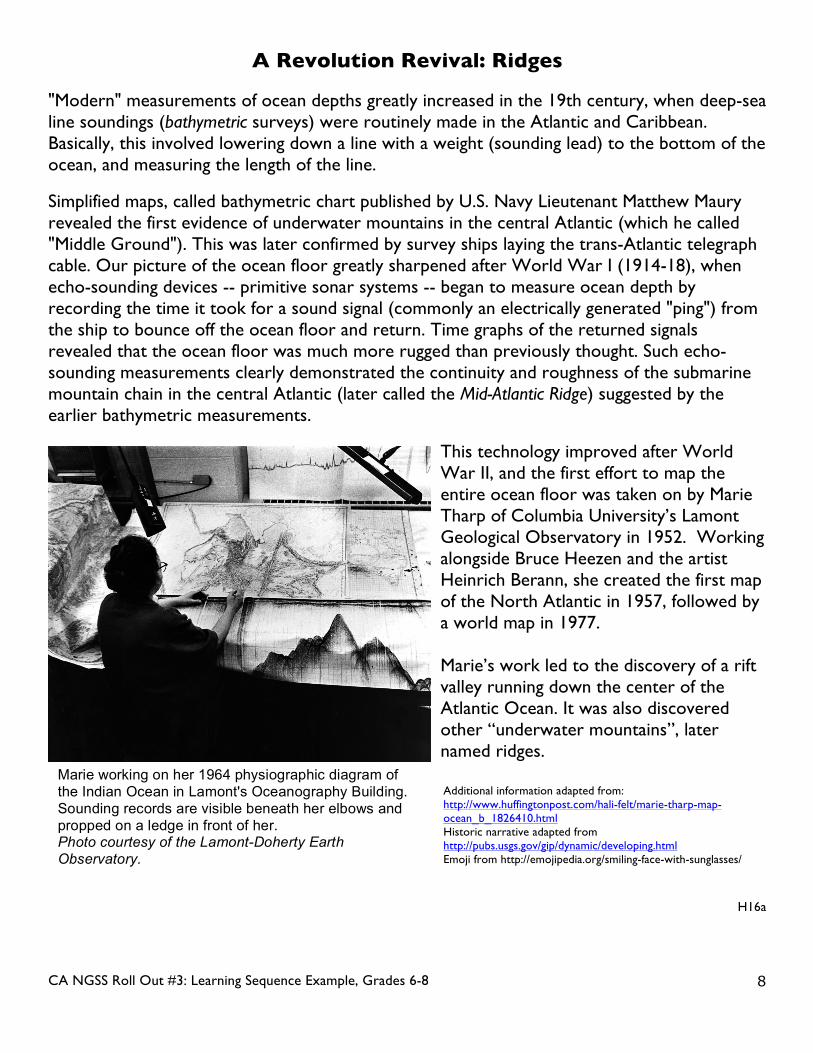
This technology improved after World War II, and the first effort to map the entire ocean floor was taken on by Marie Tharp of Columbia University’s Lamont Geological Observatory in 1952. Working alongside Bruce Heezen and the artist Heinrich Berann, she created the first map of the North Atlantic in 1957, followed by a world map in 1977. Marie’s work led to the discovery of a rift valley running down the center of the Atlantic Ocean. It was also discovered other “underwater mountains”, later named ridges. Additional information adapted from: http://www.huffingtonpost.com/hali-felt/marie-tharp-map-ocean_b_1826410.html Historic narrative adapted from http://pubs.usgs.gov/gip/dynamic/developing.html Emoji from http://emojipedia.org/smiling-face-with-sunglasses/

H16a

Marie working on her 1964 physiographic diagram of the Indian Ocean in Lamont's Oceanography Building. Sounding records are visible beneath her elbows and propped on a ledge in front of her. Photo courtesy of the Lamont-Doherty Earth Observatory.

CA NGSS Roll Out #3: Learning Sequence Example, Grades 6-8

9

A Revolution Revival: Ridges

The 1977 World Ocean Floor Panorama. It was painted by Berann and based on the previous 25 years of Marie and Bruce's work. Image courtesy of Marie Tharp Maps.

Examine the map closely and record your observations. Identify the three MOST IMPORTANT things you learned that will help your team revise and support your claim about

how the Earth has changed over time.