Embed Size (px)
Citation preview
K Y B E R N E T I K A — V O L U M E 9 (1973), N U M B E R 1
A Review of the Matrix Riccati Equation VLADIMÍR KUČERA
This paper reviews some basic results regarding the matrix Riccati equation of the optimal control and filtering theory. The theoretical exposition is divided into three parts dealing respectively with the steady-state algebraic equation, the differential equation, and the asymptotic properties of the solution. At the end a survey of existing computational techniques is given.
INTRODUCTION
As usual, R denotes the field of real numbers, R" stands for the n-dimensional vector space over R, a prime denotes the transpose of a matrix, an asterisk denotes the complex conjugate transpose of a matrix, and P _ Q means that P — Q is hermitian or real symmetric nonnegative matrix. Square brackets represent matrices composed of the symbols inside.
In order to get a better motivation for the problems to be discussed we first pose the underlying physical problem.
Given the linear, continuous-time, constant system
(1) ^ = Ax(t) + Bu(t), x(t0) = x0, at
(2) y(t) = Hx(t),
where x e R", u e Rr, and y e Rp are the state, the input, and the output of the system respectively and A, B, H are constant matrices over R of appropriate dimensions, find a control u(t) over t0 S- t _ tj which for any x 0 e R" minimizes the cost functional
(3) / - ix'(tf) S x(tf) + i Hx'Qx + u'u) df. J to
with S = 0, Q = 0.
This problem is referred to as the least squares optimal control problem and 43 it can be solved by the minimum principle of Pontryagin [ l ] , [19], [29], [32], by the dynamic programming of Bellman [1], [3], [7], [15], [19], [32] or by the second method of Lyapunov [33].
The minimum value f0 of (3) is given as
(4) A = M'o) I'(to) *(to)
and it is attained if and only if the control
(5) u(t)=-B'P(t)x(t)
is used. Here P is an n x n matrix solution of the Riccati differential equation
(6) - — = -P(t) BB' P(t) + P(t) A + A' P(t) + Q , df
P(tr) = S .
Note that this equation must be solved backward from ff to f0 in order to obtain the optimal control.
One special case is frequent in applications, namely ff -» oo, the so called regulator problem. In this particular case it may happen that P(t) approaches a finite constant, P r o , as ff -* oo, or, equivalently, as t -» — oo in (6). Then
(7) A = ix'(to) I5*, *(to) ;
the control law
(8) u(t) = -B'Pxx(t)
is independent of time and Pm satisfies the quadratic algebraic equation
(9) -PBB'P + PA + A'P + Q = 0 .
In the sections to follow we first investigate the algebraic equation (9), then the differential equation (6) and the asymptotic behaviour of the solution of (6) as t-* — oo. Finally some computing techniques for both equation (6) and (9) are surveyed.
THE QUADRATIC EQUATION
The matrix equation (9) has been extensively studied [6], [16], [22], [23], [26], [30], [36]. It is well-known that it can possess a variety of solutions. First of all (9) may have no solution at all. If it does have one, there can be both real and complex solutions, some of them being hermitian or symmetric. There can be even infinitely many solutions. Due to the underlying physical problem, however, only nonnegative
44 solutions are of interest to us. Therefore, we are mainly concerned with the existence
and uniqueness of such a solution.
In this section we summarize some long-standing as well as recent results [22],
[23], [26], [30] on (9) which will prove useful later. First of all, write
Q = C'C, S = D'D .
Then X is said to be an uncontrollable eigenvalue [13], [22] of the pair (A, B) if there
exists a row vector w + 0 such that wA = Xw and wB = 0. Similarly, X is an un-
observable eigenvalue of the pair (C, A) if there exists a vector z + 0 such that
Az = Xz and Cz = 0.
The pair (A, B) is said to be stabilizable [35] if a matrix L over R exists such
that A + BL is stable (i.e., all its eigenvalues have negative real parts), or, equi
valent^, if the unstable eigenvalues of (A, B) are controllable [13], [35].
Analogically, the pair (C, A) is defined to be detectable [35] if a matrix F over R
exists such that EC + A is stable, or, if the unstable eigenvalues of (C, A) are observ
able [13], [35].
A nonnegative solution of (9) is said to be an optimizing solution [28] if it yields
the optimal control (8); it is called a stabilizing solution [28] if the control (8)
is stable. We shall denote these solutions P0 and Ps, respectively.
Further we introduce the 2n x 2n matrix
« --ice,--:*} Unless otherwise stated we shall henceforth assume that the M matrix is diagonaliz-
able, that is, it has 2n eigenvectors. This assumption is made for the sake of simplicity
and is by no means essential.
Let
Mat = X-fii, rtM = X^i, i - 1, 2,.. ., 2n ,
and write
- й - rK:ľ where xt e R", y{ e R", ute R" and vt e R".
Thus the at is a column vector whereas the r ; is a row vector. They are sometimes called the right and the left eigenvectors of M, respectively.
It is well-known that the eigenvectors can be chosen so that
(H) rtaj - 0 . , i+j,
* 0 , i=j.
The following seems to have been proved first in [10], [26] and [30].
Theorem 1. Each solution P of (9) has the form
(12) P = YX-i ,
where
X = [xux2,...,x„],
Y = | > i , y2, • • -, yn]
correspond to such a choice of eigenvalues Xu X2, ...,X„ of M that X"1 exists.
Converselly, all solutions are generated in this way.
Proof. Let P satisfies (9) and set
K = A - BB'P,
the closed-loop system matrix. Then we infer from (9) that
PK = - Q - A'P
and hence
Let
J = X~lKX = diag(A., A2, •••, X„)
be the Jordan canonical form of K and set PX = Y Then (13) yields
(14) M Й-Й'-Й Since J is diagonal, the columns of constitute the eigenvectors of M associated
with XUX2,...,X„ and P = YX~\ The converse can be proved by reversing the arguments. •
Corollary. The matrix K = A — BB'P given by the solution (12) has the eigen
values X-t associated with the eigenvectors xt, i = 1, 2,.. ., n.
Proof. The J matrix is the Jordan form of K and X is the associated transformation
matrix. •
Theorem 2. Let Xt be an eigenvalue of M and l the corresponding right eigen-
vector. Then —Xt is an eigenvalue of M and ' ' the corresponding lefteigen-
L *d
Proof. By direct verification, making use of the identity
ИГK;-:] and the fact that a left eigenvector of M associated with X is a transposed right
eigenvector of M' associated with X. •
Note that M being a real matrix, its eigenvalues occur in quadruples {X, X*,
-X, -X*).
The procedure described in Theorem 1 is the time-domain counterpart of the
spectral factorization in the frequency domain.
We also point out that there can exist at most one stabilizing solution due to the
symmetry of the eigenvalues of M. If P s = YX~X is such a solution, then the matrix
Z*Yishermitian [30].
The following fundamental theoiems originated in [22], [23], [24].
Theorem 3. The stabilizing solution of {9) exists if and only if(A,B) is stabilizable
and Re X 4= Ojor all eigenvalues X of M.
Proof. Necessity: Suppose the stabilizing solution P s exists. It is associated with n
stable eigenvalues of M and hence no eigenvalue can have zero real part due to their
symmetrical distribution about the imaginary axis.
Moreover, the matrix L = —B'PS stabilizes A + BL, i.e., the pair {A, B)
is stabilizable.
Sufficiency: Suppose the hypothesis holds and let no stabilizing solution exist.
Then either (i) we cannot choose n stable eigenvalues of M, a contradiction, or (ii)
we can do so but the X matrix in (14) is singular.
If (ii) is the case, write z for any nonzero vector of Jr{X), the null space of X.
Since X*Y = Y*X, we have
(15) 0 = Y*Xz = X*Yz .
By virtue of (10) and (14),
(16) AX - BB'Y = XJ ,
-C'CX-A'Y =YJ.
The first equation yields
z*Y*AZz - z*Y*BB'Yz = z*Y*XJz
and hence by (15) and by the definition of z
(17) B'Yz = 0 .
But
0 = AXz - BB'Yz = XJz ,
which means that JV{X) is a J-invariant subspace of R". Hence there exists at least 47 one nonzero vector 1 e JV{X) such that
(18) Jz = jxz
where fi coincides with one of the stable eigenvalues of M. The second equation (16) postmultiplied by 2 yields
(19) -A'Yz = YJz .
Collecting (17) through (19) gives us
{Yz)' A = ->i{Yz)', Re (- /.) > 0 ,
{Yz)' B = 0 .
Thus (A, B) is not stabilizable, contradicting our hypothesis. •
Theorem 4. The stabilizing solution is the only nonnegative solution of (9) if and only if {C, A) is detectable.
Proof. Sufficiency: Assuming (C, A) detectable we shall demonstrate that any solution P of (9) is the stabilizing solution. Suppose to the contrary that a X exists such that
Kz = Xz , Re X = 0 , K = A - BB'P .
On rearranging equation (9) reads
PBB'P + PK+ K'P + C'C = 0
and hence
{X + X*) z*Pz = -z*PBB'Pz - z*C'Cz .
Since X + X* — 2 Re X = 0, the left hand side of this equation is nonnegative, while the right hand side is nonpositive. Therefore either is zero and
B'Pz = 0 ,
Cz = 0 ,
which in turn implies
Az = Xz , Re X = 0 ,
Cz = 0 .
Thus (C, A) is not detectable contradicting our hypothesis. Hence K is stable. However, there is at most one stabilizing solution, i.e., the solution P is unique.
For another proof refer to [36].
Necessity: By contradiction, suppose an undetectable eigenvalue Xi of (C, A)
exists. We shall show the existence of at least two nonnegative solutions of equation (9). One of them is the stabilizing solution P s = YX~l by hypothesis.
To form another solution P , = Yi-XT/1 we substitute the eigenvector * I of M
[ x ~| -° -1
1 associated with — A,, thus obtaining yd
X, = [z1,x2,...,x„-], Y1^[p,ylt...,y„-. Also set
X = [x2,...,xn], t=[y2,. . . , > • „ ] . Now Theorem 2 along with (11) implies that
[ z ? , 0 * ] | ~ ~ y i l = 0 , i = 2,3,...,n.
Hence z*f = 0 and
(20) ^ = r o , f j - r o ' ° > j ^ v ; Lo> x*f] L°> £*?J because X*Y = 0.
To prove that X± is nonsingular, suppose the contrary is true. Then a vector v =f= 0 exists such that z, = j£u and, consequently,
0 = z*? = v*X*f;
that is, det X*f = 0. Observing that det X*fis a principal minor of the nonnegative matrix X*Y, it is easy to see that
[xu X]*fv = X*(fv) = 0 .
This is a contradiction, however, as X is nonsingular and fv 4= 0. Thus P , does exist and is different from P s because it corresponds to a different
n—tuple of eigenvalues of M. •
Theorem 5. Stabilizability of (A, B) and detectability of (C, A) is necessary and sufficient for equation (9) to have a unique nonnegative solution which stabilizes the closed-loop system.
Proof. Sufficiency part is a well-established result in [36]; it can also be inferred from Theorems 3 and 4.
Necessity part is a simple consequence of Theorems 3 and 4. •
We note that optimality does not necessarily imply stability. Indeed, the optimizing solution minimizes the cost functional whereas the stabilizing solution makes the closed-lopp stable, and this is quite a different property. However, in control applications an optimal system which is stable as well is desirable. Conditions for this case to hold have been stated in Theorem 5, first published in [22].
Further we turn our attention to the situation when these conditions are not in force. If (C, A) is detectable and (A, B) is not stabilizable, no nonnegative solution of (9) exists. Indeed, (C, A) detectable implies by Theorem 4 that all solutions are the stabilizing solutions. But such a solution does not exist by Theorem 3.
Further let (A, B) be stabilizable and (C, A) be not necessarily detectable. In this case we characterize all nonnegative solutions of (9), see [23], [24].
Let Xt, X2, ••-, Xp, p ^ 0, be those eigenvalues of M that are also the undetectable eigenvalues of (C, A), i.e.,
AZ; = XiZi ,
CZ; = 0 .
R e 2 ( > 0 , i = l,2,..., p.
An eigenvalue A of A is called cyclic if any two eigenvectors of A associated with X are linearly dependent. We restrict ourselves to the cyclic Xb i = 1, 2 , . . . , p. Under this condition equation (9) has only a finite number of nonnegative solutions [23], [24]. Otherwise nondenumerable many nonnegative solutions exist as the example A = B = I, C = 0, w > 1 shows, see [23], [24] for details.
Define
(21) <€ = {XUX2,...,X„}
and write <€k, k = 1, 2, ... for the subsets of <€. Note that all -X„ i = 1,2, ...,p must be used to form the stabilizing solution if it exists, since Re (-A;) < 0.
Write Pk for the solution of (9) which is generated from the stabilizing solution by replacing all —Xi with Xh Xt e <£k.
The theorems below have originally been proven in [23], [24].
Theorem 6. Suppose the stabilizing solution of equation (9) exists. Then the set of all Pkform the class of all nonnegative solutions of (9), and there are exactly 2P
such solutions.
Proof. Existence of all Pk can be proved in an identical manner as the existence of Pj in the "if" part of the proof of Theorem 4.
To see that no other nonnegative solution of (9) exists, firstly substitute an eigenvalue X e <€ for the eigenvalue — X. Arguing as in [23] we conclude that either X*Y >. 0 or X is singular and hence the corresponding solution cannot be nonnegative.
Secondly make the substitution of an eigenvalue X, Re X ^ 0, for an eigenvalue p, Rep < 0, -n =t= X. Applying (11) and Theorem 2 we conclude that X*Y4= Y*X and such a solution cannot be nonnegative, either.
The number of solutions follows from the fact that there are 2P subsets of a set consisting of p elements. •
Remark. If the M matrix is not diagonalizable, a more refined analysis in [23]

50 shows that, in general, there exist
fhi + s.) i = l
nonnegative solutions, where
Czi+j = 0 , jf = 0, 1 , . . . , s( - 1 ,
* 0 , j = Si
and Azi + j = A;Z; , j = 0 ,
= ^ i + j + Zi + j - l , J = 1, 2, ..., S; - 1 .
Theorem 7. Any two nonnegative solutions Pk, P ( of (9) satisfy
(22) Pk = Pt if and only if <$k s V,.
Otherwise speaking, the set of all noiinegative solutions constitute a distributive lattice with respect to the partial ordering ^ . P0is the smallest nonnegative solution (the zero element of the latice) and Ps is the largest nonnegative solution (the identity element of the lattice).
Proof. The claim hinges on the observation that the family of subsets %k constitute a distributive lattice with respect to the partial ordering by inclusion and that (22) is an isomorphism.
In particular, c€k = 0 implies Pk = Ps whereas Vk = (6 implies Pk = P0. The relation (22) itself follows from (20). •
Note that if (C, A) is detectable then V = 0 and hence P0 = Ps. However, (C, A) undetectable implies that V 4= 0 and hence P„ =£ Ps; the two solutions never coincide:
The physical interpretation of different real nonnegative solutions is as follows [26]. Each nonnegative solution is a conditionally optimizing solution of (9), the condition being a certain degree of stability. Specifically, Pk stabilizes the undetectable eigenvalues of (C, A) included in <%k and no others. Equation (9) thus contains the optimal solutions for all degrees of stability [23], [24], [26]. The idea that the more undetectable eigenvalues is stabilized the higher is the cost f is made rigorous via the concept of lattice.
THE DIFFERENTIAL EQUATION
In this section we summarize some fundamental results on the Riccati equation (6) which are scattered in the literature [1], [6], [8], [9], [15], [17], [19], [20], [32], [36].
The well-known theorem on differential equations guarantees only local existence and uniqueness for the solution of (6); without further analysis we cannot conclude existence over t0 = t ^ t{ because of the phenomenon of finite escape time.
Nonetheless, the following is proved in [6], [8], [9], [15], [36].
Theorem 8. Let P(t, S, t() be the solution of (6) which passes through S at t = t(. Then given any t0, P(t, S, t() exists and is unique on t0 S= t :§ tt regardless of S.
Proof. In view of the local existence the P(t, S, t() exists for some t ^ t(. Let ^(f, t() be the transition matrix of A. Then
P(t, S, t() = W'(t, tt) S T(t, tt) +
+ fV ( f , T) [Q - P(T, S, I,) BB' P(r, S, iv)] W(t, T) dx ^
^ W'(t, t() S V(t, t() + f V(f, t) 6 y(t, T) dr ,
which can be verified by elementary differentiation. The a priori upper bound above provides a Lipschitz constant on any finite interval t0 g t g tt no matter how large. Hence P(t, S, t() exists and is unique globally for any S. •
Theorem 9. For any t0 S t ^ tf 0«d any S ji 0,
(23) P(r, S, tf) ^ 0 .
Proof. If P(t, S, t() satisfies (6), then P*(t, S, t() does so. Hence P(t, S, t() is a hermitian matrix. Moreover, using (4), we obtain (23) since
/„ = min / ^ 0 . •
Theorem 10. The solution P of (6) enjoys the following properties:
(24) P(t0, 0, f,) S P(t0, 0, h)
for any t0 S ti ^ t2,
(25) % 0 , l t ) ^ ( f l ! 0 , ( t )
for any t( 5£ t2 <; ff,
(26) P(t, Su t() S P(t, S2, t()
for any nonnegative S( :g S2 and t ^ t(.
Proof. Regarding (24), we have
x0 P(t0, 0, t() x0 = min (x'Qx + u'u) dt ^ u J to
g min (x'Qx + u'u) dt = " J to
= x0 P(f0, 0, t2) x0
for any x0 e R".
52 Regarding (25), the substitution tt — t = T in (3), gives us
P(t0, 0, tt) = P(0, 0, ff - t0)
and hence (25) follows from (24) on identifying t0 with tx and f2 in turn. Finally, (26) is obvious since increasing the terminal penalty results in increased
cost functional (3). We conclude this section by emphasizing that we are not concerned with stability
of the optimal closed-loop system since the control problem is defined over a finite interval.
ASYMPTOTIC BEHAVIOUR OF THE SOLUTION
Now we let ff -* oo and investigate the properties of P(t) over the half-line t0 =
< t < oo. Since the Riccati equation coefficients are independent of time, P(t0, S, ff) = = P(0, S, ff — f0) and it makes no difference to consider t -» — oo and the half-line — oo < f < ff instead. The first arrangement reflects the time evolution of the system, whereas the other is convenient from the computational point of view.
It is easy to see that additional assumptions will be required to keep P(f) from passing off to infinity.
Theorem 11. If (A, B) is stabilizable, then the solution P(t, S, ff) of (6) is bounded on — oo < f < ff regardless of S and ff.
Proof. Consider a control
u(t) = Lx(t), t0<t',
such that the closed-loop system matrix A + BL is stable. Then
x'0 P(t0, S, ff) x0 = min [x'(ff) S x(tt) + (x'Qx + u'u) df] < " J <0
< f (x'Qx + u'u) df = x'0 W(t0, t) x0
J to
since x(t{) -> 0 as ff -* oo, and x0 = x0.
Here IV(f0, f) is a finite matrix over R for any f < ff. Hence P(f0, S, f) is bounded from above for any f0, any f0 < f < co, and any S.
Equivalently, P(f, S, ff) is bounded for any ff, any — oo < f = ff, and any S. • Theorem 11 is proved in [36] without any appeal to variational ideas. Our proof,
however, is considerably simpler and more intuitive.
First the asymptotic properties of P(f, 0, ff) will be discussed and existence of an equilibrium solution of (6) deduced, see [15], [36].

Theorem 12. If (A, B) is stabilizable, then
lim P(t, 0, t{) = PK , <->-CO
a finite nonnegative matrix.
Moreover, POT is a fixed point solution of (6),
P„ = P(t, Px, t{).
Proof. By Theorem 10, (25), P(t, 0, rf) is monotone nondecreasing in t in the ordering of nonnegative matrices. Further Theorem 11 implies that P(t, 0, tt) is bounded from above and consequently there exists a finite matrix Px — 0 so that P(f, 0, tf) - ^ P t t as f-> - o o .
Since P ^ is independent of t, it satisfies both (6) and (9), that is, PM = = P(t, Px, t{). D
We remark that even if the stabilizing solution P s of (9) exists, Pm = P s need not be true. Naturally, there arises the question: To which nonnegative solution of (9) does P(t, 0, ff) converge? The answer is contained in the two theorems below [26], [36].
Theorem 13. / / (A, B) is stabilizable, then
Px=Pa-
Proof. Since S ^ 0, we infer from Theorem 10, (26) that P(t, S, t{) = P(t, 0, tf) for any S. Thus, as t -> — oo, P(t, 0, t{) -> P0, the smallest nonnegative solution of (9). D
Theorem 14. If (A, B) is stabilizable and (C, A) is detectable, then
PK= Po = ps.
Proof. By hypothesis Theorem 5 implies that equation (9) possesses the unique nonnegative solution P„ = Ps. Thus the claim follows from Theorem 13. ' •
Now we generalize and consider the asymptotic behaviour of P(t, S, t{) rather than of P(t, 0, tf). Theorem 12 is not known to hold for arbitrary nonzero S = 0 as yet, even though some conjectures so that effect has been made [26]. The difficulty stems from the fact that P(f, S, t{) is not monotone nondecreasing in t.
We avoid the impasse by assuming that not only (A, B) is stabilizable but also Re X 4= 0 for all eigenvalues X of M. This is equivalent to the assumption that P s
exists.
Thus we are ready to prove the original results of this paper.
54 Theorem 15. If P s exists then
lim P(t, S, t{) = Px , f-»-oo
a finite nonnegative matrix. Moreover, P m is a fixed point solution of (6),
P m = P(t, Px, t{) .
Proof. For S = 0 the theorem reduces to Theorem 12. Thus it will suffice to show that the term x'(t{) S x(t{) approaches zero as tf -» oo.
By the assumption of Re X 4= 0 this term goes either to zero or to infinity. The latter case is not possible, however, since by Theorem 11 the cost is bounded from above. •
Observe again that, in general, Px need not coincide with either P s or P0. And again we ask: To which nonnegative solution of (9) does P(t, S, ff) converge?
We have to take S = D'D into account. Let p,u \i2,..., nq, q = 0, be those eigenvalues of M that are also the undetectable eigenvalues of (D, A), i.e.,
Azt = HiZf,
Dz{ = 0 ,
Re ^ = 0 , i = 1, 2 , . . . . q.
Define
in accordance with (21).
Theorem 16. i / P s exists then
P*=Pk
if and only if <£k = «" n 9 .
Thus P(t) can be made to approach any nonnegative solution Pk of (9) by taking an appropriate S.
Proof. To demonstrate the interaction of S and Q assume first that all undetectable eigenvalues Xt of (C, A) belong to <?, where Si corresponds to an arbitrary S ^ 0. Then Dzt = 0 and hence
lim P(t, S, tf) = lim P(t, 0, ff) = P0 «-»-» t-+-oo
by Theorem 13. Note that P0 is generated by the set ^ = ^ n S. Second, let one undetectable eigenvalue Xt of (C, A) does not belong to S. Then
Dzx 4= 0 and lim P(t, S, tf) = P j

where P t is generated by the set <€x = e€ — {Aj = <& n 9. It is so since otherwise
the cost would be infinite due to the term x'(tr) D'D x(t(). Consequently, Px = Pk if and only if <€k = <€ n 9. •
Observe that Px is the smallest nonnegative solution of the lattice generated by the set <€ n 9 rather than by the <€ itself.
Theorem 17. If (A, B) is stabilizable and (C, A) is detectable, then
px= p o = p s
for any S >. 0.
Proof. By Theorem 5, equation (9) has the unique nonnegative solution P„ = P s . Thus our claim is proved by referring to Theorem 16. •
From the computational viewpoint Theorem 16 renders it possible to find an S such that P(t, S, t() will approach a desired equilibrium solution P^ . In particular,
P K = P s if and only if <$ n 9 = 0 and
The relation px = Po if and only if <€ n 9 = <£ .
lim P(t, S,t() = Pko<g n 9 = <€k
is an equivalence and, therefore, it induces a decomposition of the cone of non-negative matrices S into equivalence classes. Each class contains those S that make P(t, S, t{) converge towards a particular Pk. Thus we see that Px is not a continuous function of 5 [26]. This is an observation of crucial importance in computations.
COMPUTATIONAL TECHNIQUES
This section is concerned with the computational aspects. Various techniques of finding a solution to equations (6) and (9) are reviewed. It is very difficult to label a particular method as being superior to the others. Each method may prove better in one application but it may fail in another. Our aim is to bring the most important methods to the reader's attention and indicate their applicability, advantages and objections.
Computing the solutions of the algebraic equation
(j) Eigenvector Solution
This method has been reported in [2], [10], [12], [23], [26], [27], [30] and its essentials are stated in Theorem 1. Apart from its theoretical importance, it is computationally promissing as efficient and accurate algorithms to compute eigenvalues of a matrix are now available.
56 This is the only method for computing any solution of (9), no matter whether it is nonnegative or not.
(it) Iterative Solution
This technique has been first reported in [4], [20], [21] and is believed to be one of the best methods to find the stabilizing solution of (9). It is assumed that (9) possesses a unique nonnegative (stabilizing) solution Ps, which is being found by successive linear approximations.
Let Pj, j = 0, 1 , . . . be the unique nonnegative solution of the linear algebraic equation
(27) PJKJ + K'JPJ + C'C + L'JLJ = 0
where, recursively,
Lj = -B'Pj^, j = 1 ,2 , . . . ,
Kj = A + BLj
and where L0 is chosen such that the matrix K0 = A + BL0 is stable. Then
Ps^Pj+1 ^Pj^..., j = 0,1,..., and
(28) lim Pj = Ps. j'-*co
Indeed, K0 being stable, (27) has a unique nonnegative solution P0 . This yields a Kx
and, in turn, a Pt. A little manipulation with the associated cost functionals reveals that Ps i^ Pi <z P0. P t being bounded, Kt is stable etc. A theorem on monotonic convergence of nonnegative matrices guarantees the existence of a limit. Then (27) is identical to (9) when j -> oo and (28) holds by uniqueness of Ps.
The method provides monotonic and quadratic convergence. In fact, it is an ingenious modification of Newton's method reported in [5].
(iii) Solution Using the Sign Function
This method is described in [31] and can be viewed as a simplification of (i) to find the stabilizing solution.
The matrix function sign Z is defined in [31] by
signZ = lim Z t + 1 , fc-»oo
where
z^i-K-^ + z*"*1). fc-o,i,..., z0 = z.
Define also sign* Z = i ( 7 + s ignZ) .
Then assuming K = A — BB'P is stable and defining a matrix V by
KV + VK' + BB' = 0, it is easy to check that
r/, -V i p . o - ip -VP,V - | [_p, / - pVJ Lo, -K'J L-p. I J
Hence
~--fc;:^T-r_-~l_-(I-pF)p> /-pVJ
and P follows immediately if V~i exists. Note that M is not taken through a complete spectral factorization, but into two
parts only. Computing the solution of the differential equation
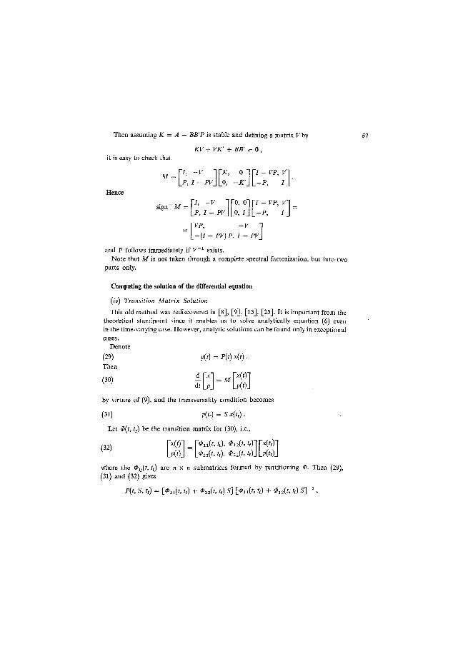
(iv) Transition Matrix Solution
This old method was rediscovered in [8], [9], [15], [25]. It is important from the theoretical standpoint since it enables us to solve analytically equation (6) even in the time-varying case. However, analytic solutions can be found only in exceptional cases.
Denote (29) p(t) = P(i)x(t). Then
(30) A M = ^ P . . l dtlpj UoJ
by virture of (9), and the transversality condition becomes
(31) p(t{) = S x(t{).
Let <P(t, t{) be the transition matrix for (30), i.e.,
(32) [X01 __[-<_,(.t{), *12(t,t{)irx(t{)i K UoJ L*2i(t,tt),*22(utt)]\j(tt)j where the 4>tJ(t, t{) are n x n submatrices formed by partitioning <P. Then (29), (31) and (32) gives
p(r, s, t{) = [__,(,, <f) + $22(t, t{) S] [_ tt(t, t{) + $i2(t, t{) sy1.
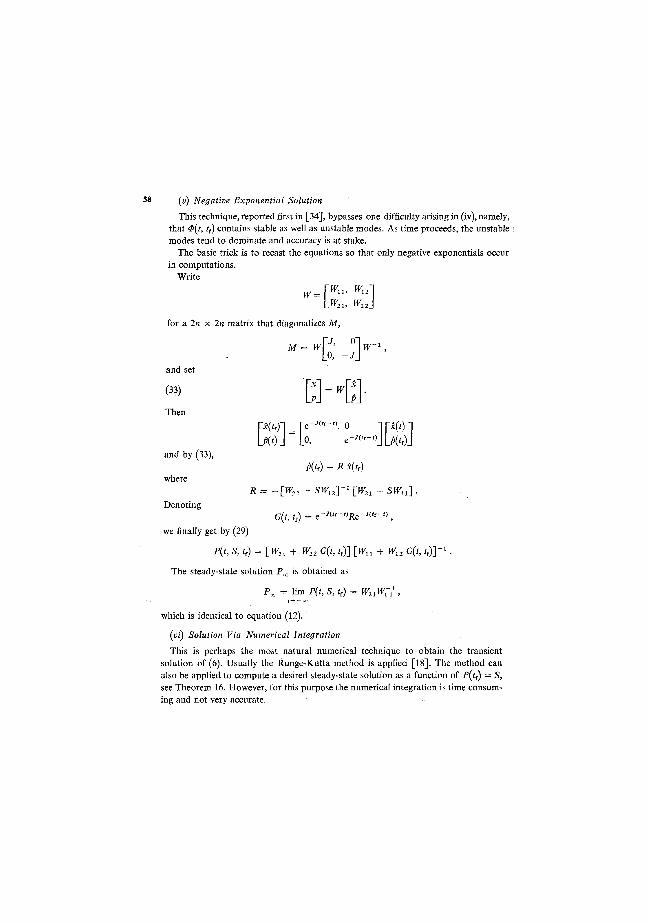
5 8 (v) Negative Exponential Solution
This technique, reported first in [34], bypasses one difficulty arising in (iv), namely, that <P(t, ff) contains stable as well as unstable modes. As time proceeds, the unstable modes tend to dominate and accuracy is at stake.
The basic trick is to recast the equations so that only negative exponentials occur in computations.
Write
for a 2« x 2n matrix that diagonalizes M,
\WU, W12l
[w21, w22\ i M,
Lo, -J\ and set
(33) £]--« Then
and by (33),
where
Denoting
Yx(tt)l = rc-^-'\ o irx(t)i
ml Lo, e-c<HL/Xíf)J
p(tt)~Rx(tt)
R = -[W22 - SW12YX [W21 - SWtl] .
G(t, ř f) = t''tft.-nR(rHu-t> t
we finally get by (29)
P(t, S, tt) = [W21+ W22 G(t, tt)] {Wtl + W12 G(t, t ^ 1 .
The steady-state solution Px is obtained as
Px = lim P(t, S, ff) = W21W^ , f-»-oo
which is identical to equation (12).
(vi) Solution Via Numerical Integration
This is perhaps the most natural numerical technique to obtain the transient solution of (6). Usually the Runge-Kutta method is applied [18]. The method can also be applied to compute a desired steady-state solution as a function of P(tt) = S, see Theorem 16. However, for this purpose the numerical integration is time consuming and not very accurate.
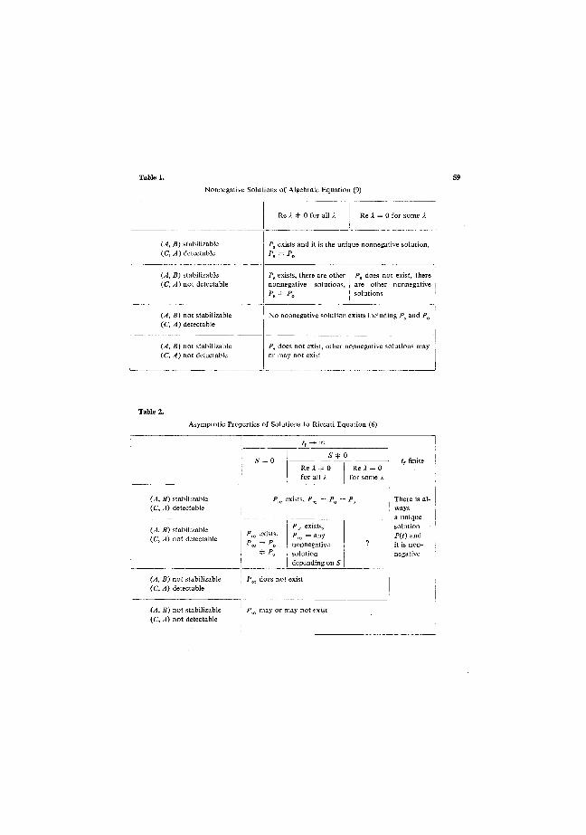
ТаЫе 1.
Nonnegative Solutions of Algebraic Equation (9)
Re X Ф 0 for all X Re X — 0 for some X
(A, B) stabilizable (C, A) detectable
Ps exists and it is the unique nonnegative solution, Ps =P0
(A, B) stabilizable (C, A) not detectable
Ps exists, there are other nonnegative solutions,
P*4=Fo
Ps does not exist, there are other nonnegative solutions
(A, B) not stabilizable (C, A) detectable
No nonnegative solution exists including Ps and P0
(A, B) not stabilizable (C, A) not detectable
Ps does not exist, other nonnegative solutions may or may not exist
Asymptotic Properties of Solutions to Riccati Equation (6)
t{ -»• 00
t{ finite 5 = 0 S Ф O
t{ finite 5 = 0 Re X Ф 0
for all X
ReA = 0
for some X
t{ finite
(A, B) stabilizable (C, A) detectable
Pm exists, Pm = P0 = Ps There is al-ways a unique solution P(t) and it is non-negative
(A, B) stabilizable (C, A) not detectable
Pm exists, pm = p „
* Ps
Pm exists, Pm = any nonnegative solution depending on 5
1
There is al-ways a unique solution P(t) and it is non-negative
(A, B) not stabilizable (C, A) detectable
Pm does not exist
There is al-ways a unique solution P(t) and it is non-negative
(A, B) not stabilizable
(C, A) not detectable Pm may or may not exist
There is al-ways a unique solution P(t) and it is non-negative
To conclude this section we mention yet another group of methods to solve (9). The common feature is that equation (9) is transformed into a recurrent algebraic equation [14] whose solution coincides with the unique nonnegative solution of (9). The resulting matrix recurrent equation is then straightforward to solve.
CONCLUSIONS
The reader will have noticed that the interrelations of different nonnegative solutions of (9) are quite complicated. Letting ff -> oo and studying the asymptotic behaviour of (6) makes the matters even worse. Therefore the following Tables 1 and 2 are provided to summarize the results for equations (9) and (6), respectively.
We also stress that the aim of the paper was to study the matrix Riccati equation in general and not to restrict ourselves to common engineering applications. This approach in turn provides a deep insight into the problem of least squares control and the engineer is well prepared to cope with ill-behaved solutions.
(Received June 5, 1972.)
REFERENCES
[1] M. Athans, P. L. Falb: Optimal Control. McGraw-Hill, New York 1966. [2] R. W. Bass: Machine Solution of High-Order Matrix Riccati Equations. Douglas paper 4538. [3] R. Bellman: Dynamic Programming. Princeton University Press, Princeton, N . Y. 1957. [4] S. P. Bingulac, M. R. Stojic, N. Cuk: On an Iterative Solution of Time-Invariant Riccati
Equation. In: Prepr. JACC, St. Louis, Miss., 1971, 178—182. [5] T. R. Blackburn: Solution of the Algebraic Matrix Equation Via Newton-Raphson Iteration.
In: Prepr. JACC, Ann Arbor, Mich., 1968, 940—945. [6] R. W. Brockett: Finite Dimensional Linear Systems. John Wiley, New York 1970. [7] A. E. Bryson, Yu-Chi Ho: Applied Optimal Control. Bleisdell, Waltham, Mass. 1969. [8] R. S. Bucy: Global Theory of the Riccati Equation. J. Comp. System Sci. 1 (December 1967),
4, 349-361 . [9] R. S. Bucy, P. D. Joseph: Filtering for Stochastic Processes with Applications to Guidance.
Interscience, New York 1968. [10] J. J. O'Donnell: Asymptotic Solution of the Matrix Riccati Equation of Optimal Control.
In: Proc. 4th Ann. Allerton Conf. Circuit and Syst. Theory, Urbana, 111., 1966, 577—586. [11] S. E. Dreyfus: Dynamic Programming and the Calculus of Variations. Academic Press,
New York 1965. [12] A. F. Fath: Computational Aspects of the Linear Optimal Regular Problem. Trans. IEEE
AC-14 (October 1968), 547-550. [13] M. L. J. Hautus: Stabilization, Controllability and Observability of Linear Autonomous
Systems. Nederl. Akad. Wetensch., Proc. Ser. A73 (1970), 448—455. [14] K. L. Hitz: Relations Between Continuous-Time and Discrete-Time Quadratic Minimization.
Ph. D. Thesis, The University of Newcastle, Australia, 1970. [15] R. E. Kalman: Contributions to the Theory of Optimal Control. Bol. Soc. Mat. Max. J
(1961), 102-119. [16] R. E. Kalman: When Is a Linear Control System Optimal? Trans. ASME, J. Basic Engr.
86D (March 1964), 5 1 - 6 0 .

[17] R. E. Kalman, R. S. Bucy: New Results in Linear Prediction and Filtering Theory. Trans. ASME, J. Basic Engr. 83D (1961), 95 -100 .
[18] R. E. Kalman, T. S. Englar: A Users Manual for the Automatic Synthesis Program. NASA Rept. CR-475, June 1966.
[19] R. E. Kalman, P. L. Falb, M. A. Arbib: Topics in Mathematical System Theory. McGraw-Hill, New York, 1969.
[20] D. L. Kleinman: On the Linear Regulator Problem and the Matrix Riccati Equation. MIT Electronic Systems Lab., Cambridge, Mass, Rept. ESL-R-271, June 1966.
[21] D. L. Kleinman: On an Iterative Technique for Riccati Equation Computations. Trans. IEEE AC-13 (February 1968), 114-115.
[22] V. Kucera: A Contribution to Matrix Quadratic Equations. Trans. IEEE AC-17 (June 1972), 344-347.
[23] V. Kucera: On Nonnegative Definite Solutions to Matrix Quadratic Equations. In: Proc. 5th IFAC Congress Vol. 4, Paris, 1972. Also Automatica 7 (July 1972), 413-423.
[24] V. Kucera: The Discrete Riccati Equation of Optimal Control. Kybernetika 8 (1972), 430—447.
[25] J. J. Levin: On the Matrix Riccati Equation. Trans. Am. Math. Soc. 10 (1959), 519-524. [26] K. Martensson: On the Matrix Riccati Equation. Information Sci. 3 (1971), 1, 17—49. [27] A. G. J. McFarlane: An Eigenvector Solution of the Linear Optimal Regulator Problem.
J. Electron. Contr. 14 (June 1963). [28] B. P. Molinari: The Stabilizing Solution of the Matrix Quadratic Equation. To appear
in SIAM J. Control 10 (1972). [29] L. S. Pontryagin at al.: The Mathematical Theory of Optimal Processes. Interscience,
New York 1961. [30] J. E. Potter: Matrix Quadratic Solutions. SIAM J. Appl. Math. 14 (May 1966), 3, 496-501 . [31] J. D. Roberts: Linear Model Reduction and Solution of the Algebraic Riccati Equation
by Use of the Sign Function. To appear in Trans. IEEE AC-17 (1972). [32] A. P. Sage: Optimum Systems Control. Prentice-Hall, Englewood Cliffs, N. J. 1968. [33] V. Strejc: State Space Synthesis of Discrete Linear Systems. Kybernetika 8 (1972), 83 -113 . [34] D. R. Vaughan: A Negative Exponential Solution for the Matrix Riccati Equation. Trans.
IEEE AC-14 (February 1969), 7 2 - 7 5 . [35] W. M. Wonham: On Pole Assignment in Multi-Input Controllable Linear Systems. Trans.
IEEE AC-12 (December 1967), 660-665. [36] W. M. Wonham: On a Matrix Riccati Equation of Stochastic Control. SIAM J. Control 6
(1968), 4, 681-698.
Ing. Vladimir Kucera, CSc, Ustav teorie informace a automatizace CSAV (Institute of Information Theory and Automation — Czechoslovak Academy of Sciences), Vysehradskd 49, 128 48 Praha 2. Czechoslovakia.