A Review of Evolutionary Graph Theory

With Applications to Game Theory

Paulo Shakarian

Network Science Center and Dept. of Electrical Engineering and Computer Science,

United States Military Academy, West Point, NY 10996

Patrick Roos

Dept. of Computer Science, University of Maryland, College Park, MD 20740

Anthony Johnson

Network Science Center and Dept. of Mathematical Sciences, United States MilitaryAcademy, West Point, NY 10996

Abstract

Evolutionary graph theory (EGT), studies the ability of a mutant gene toovertake a finite structured population. In this review, we describe the origi-nal framework for EGT and the major work that has followed it. This reviewlooks at the calculation of the “fixation probability” - the probability of amutant taking over a population and focuses on game-theoretic applications.We look at varying topics such as alternate evolutionary dynamics, time tofixation, special topological cases, and game theoretic results. Throughoutthe review, we examine several interesting open problems that warrant fur-ther research.

Keywords: evolutionary dynamics; structured population; game theory;fixation probability; time to fixation

1. Introduction

Evolutionary graph theory (EGT), introduced by [23], studies the abilityof a mutant gene to overtake a finite structured population. The repro-duction of the individuals in the population is modeled as a stochastic pro-cess. The structure of the population is represented as a directed, weighted

Preprint submitted to BioSystems October 2, 2011

graph called an evolutionary graph (EG). Since its introduction, numerousresults on EGT, both analytical and experimental, have been produced. Ad-ditionally, several extensions to the model have been proposed, includinggame-theoretic ones. The application of EGT to game theory has providedresearchers new insight about the evolution of cooperation and other game-theoretic concepts in structured populations. In this review, we present theoriginal model of [23] and various extensions. We also summarize major re-sults in EGT (both analytical and experimental), including those relatingto game theory. Throughout this review, we pose several open questions inEGT that would be relevant for future research.

This review is organized as follows. In Section 2, we introduce the originalmodel, discuss computation of fixation probability, and describe the standardgame theoretic extensions. This is followed by a presentation of results con-cerning the computation of the fixation probability in Section 3 for graphsof certain topologies - including the large class of undirected EG’s. We thenturn to the related problem of mean time to fixation in Section 4. Thenwe describe how some of the results relating to fixation probability changeunder alternative model dynamics in Section 5. We then survey more ad-vanced game theoretic extensions in Section 6. Finally, in Section 7, wepresent other major extensions to EGT including the study of bi-level EG’sand EG’s whose topology change over time.

2. The Model

Consider a population of N individuals where there is no specified graph-structure relating them to each other (this is known as a well-mixed pop-ulation). The Moran Process of [29] is a stochastic process used to modelevolution in such a population. It is defined as follows. At each time-stepa randomly selected individual is chosen to reproduce. Then, a second in-dividual is chosen at random to die – replaced by a duplicate of the firstindividual. If all of the members of the population are identical (termedresidents with fitness 1), and a mutant is introduced at random in the pop-ulation (with fitness r, where r = 1 is the special case of neutral drift), theprobability that the mutant will eventually overtake the population is knownas the fixation probability (the opposite event - that all mutants die out - iscalled extinction and a population with a lower fixation probability is deemedmore evolutionarily stable as it is resistant to invasion by a mutant). This

2

probability, ρ1, arising from this N original Moran Process, is often termedthe Moran probability and can be solved for exactly (see equation 1).

ρ1 =1− 1/r

1− 1/rN(1)

In the original work that introduced EGT [23], Lieberman et al. generalizethe model of the Moran Process by specifying relationships between the Nindividuals of the population in the form of a directed, weighted graph. Weshall use the symbol V to denote the set of individuals. We can think ofthese individuals as vertices in a graph. The edges of the graph are specifiedby the adjacency matrix W = [wij], where for vertices vi, vj, the quantitywij specifies the weight of the directed edge from vi to vj. As this is anevolutionary graph (EG), wij corresponds to the probability that, if vi isselected to reproduce then it replaces vj (note that for all vi, wii = 0). Hence,for any given vi,

∑j wij = 1. The earlier work of [46] proves that, in such a

structure if ∀vi, vj ∈ V we have wij = wji, then the fixation probability fora randomly placed mutant is ρ1. A similar result was proved in [24]. In [23],this result is extended for a wider variety of EG’s where ∀vi,

∑j wij =

∑j wji.

This type of EG is known as isothermal. Consider the following theorem.

Theorem 1 (Isothermal Theorem [23]). An EG is isothermal iff the fix-ation probability of a randomly placed mutant is ρ1.

Hence, for EG’s that are not isothermal, the fixation probability of the evo-lutionary process is not only dependent on the fitness of the mutant (as inthe Moran Process), but also on the structure of the graph.

2.1. Properties of Fixation Probability

Many researchers (such as [9] and [26]) have studied the problem of com-puting the probability of fixation given that a certain subset of vertices aremutants. If the mutants inhabit set C ⊆ V , then this probability is writtenPC . As the calculation of the fixation probability (ρ) for an EG is deter-mined based on a uniformly picked vertex, we have the following relationshipbetween ρ and P :

N · ρ =∑i

P{vi} (2)

Note that although these two problems are closely related, they have ratherdifferent intuitions. The fixation probability ρ provides insight into a graph

3

of a certain topology. For example, researchers often refer to graphs with alow value for ρ as being “evolutionary stable” as the toplogy of the graphseems to be resistant to a mutant invasion. The fixation probability PC onthe other hand tells us something about a set of vertices C. For example,identifying a certain subset C of a graph that has a higher fixation probabilitymay cause a user to take a certain action regarding those vertices (dependenton the domain).

If the graph is not isothermal, but if we are under neutral drift, fixationprobability PC is additive. This was proven for the special case of undirectedgraphs in [8] and proved for general, weighted, directed graphs by the authorsof this review in [45].

Theorem 2 (Additive Under Neutral Drift [45]). When r = 1 for dis-joint sets C,D ⊆ V , PC + PD = PC∪D.

This additive result says that, under neutral drift, determining a subsetof indivdiuals in the population that maximize fixation probability is not(polynomially) harder than determining the fixation probability. Further,when we fix the topology of the graph, we find that for some subset ofvertices C, that the fixation probability under neutral drift is a lower boundfor the fixation probability when r > 1.

Theorem 3 (Neutral Drift as a Lower Bound [45]). For a given set C,

let P(1)C be the fixation probability under neutral drift and P

(r)C be the fixation

probability calculated using a mutant fitness r > 1. Then, P(1)C ≤ P

(r)C .

By Theorem 2 and Equation 2, we observe that under neutral drift ρ =1/N regardless of the topology of the graph - even with directed and weightededges. Hence, Theorem 3 tells us that for r > 1 we have ρ ≥ 1/N . Thisparticular observation is independently noted in [20]. In [25] the authorsobserve in their experiments that fixation probability monotonically increaseswith r. Based on these observations and Theorem 3, we have the followingconjecture.

Conjecture 2.1. Fixation probability is montonic in r.

This conjecture seems natural and is supported by experimental results.However, a formal proof is currently lacking.

4

2.2. The Complexity of Computing Fixation Probability

As we can appeal to the Moran probability only in the case of an isother-mal graph, we must resort to other calculations to determine ρ or P . Usingthe following set of constraints, we can solve directly for any PC (hence, ρ aswell by Equation 2).

PC =

∑vi∈C

∑vj /∈C(r · wij · PC∪{vj} + wji · PC−{vi})∑vi∈C

∑vj /∈C(r · wij + wji)

. (3)

These constraints originally appeared in [43] for the case of an undirectedEG, but applies to the general case as it follows directly from the rules ofdynamics. However, the number of constraints and variables is equal to thenumber of mutant-resident formations in the graphs, which is intractable forlarge N . In fact, [23] presents a decision problem related to computing thefixation probability that is claimed to be as hard as any problem in the com-plexity class NP (the class of nondeterministic polynomial time computableproblems). In [9, 8] the authors attempt to reduce the number of constraintsby finding automorphisms in the graph. Based on automorphism, the authorsare able to calculate the exact number of possible mutant-resident formations(MRF’s). Since this number gives the size of the system of linear equationsfor the fixation probability and in general increases with the difficulty of solv-ing this system, the measure may be a useful indicator in deciding whetherto undertake an analytical approach to solving for the fixation probability ona given graph. The authors then show that even in the special case of undi-rected EG’s, if the graph contains a vertex of degree of at least 3, that thereis a non-zero probability that the dynamics will evolve to any of the MRF’s(except in the trivial cases where C = V or C = ∅).1 We note that for thegeneral case, this still leads to an intractable number of constraints. Further,finding graph automorphisms is also a non-trivial problem in the general case(see [50] for the latest complexity results on graph automorphism).

We note that the problem proven to be NP-hard by [23] is actually moregeneral than a standard computation or ρ using their model. As for anupper bound on complexity, Equation 3 only tells us that this problem can

1There is the exception of an alternating state where every edge connects a mutant-resident pair. This state cannot be reached if it exists. We would like to thank ananonymous reviewer for pointing this out.

5

be solved in exponential time. Hence, the issue of finding a tight bound onthe complexity for computing fixation probability is still an open problem.

Open Problem 2.1. What is the computational complexity of determiningρ in an arbitrary evolutionary graph?

Open Problem 2.1 is important to the study of evolutionary graph the-ory as virtually all current work in this area is perofrmed with simulation.Often, it has been found that this approach does not scale well for largegraphs. Properly identifying the complexity class of this problem may pro-vide insight into the development of a more efficient and scalable approach,perhaps broadening the appeal of this paradigm.

What about the computational complexity of finding PC - the fixationprobability given seet C ⊆ V are mutants and the rest are residents? Clearly,

as ρ =∑

vi∈V P{vi}

N, solving N instances of PC can give us ρ. However, a

reduction going in the opposite direction seems less likely, so it is possiblethat determining PC may be more difficult than finding ρ.

Despite the computational difficulty of determining the fixation proba-bility in the general case, there are several special classes of EG’s where wehave analytical solutions (or at least good approximations). We review manyof these special cases in the next section. To address the issue of computa-tion of the fixation probability in the general case (i.e., to confirm analyticalapproximations), most work we review resorts to simulation methods viaMarkov Chain Monte Carlo (MCMC). These simulations generally rely ona direct application of the model we have already described (see [43] for apseudocode algorithm). However, as the size of the graph increases, evensuch simulations may become impractical. In [4], the authors address theissue of increasing the speed of such simulations. Their main technique forthe general case is to stop the simulation early if the number of mutants inthe population exceed a certain threshold (hence that particular simulationwould be considered to have reached fixation). They determine this thresh-old by finding the conditional probability that mutants spread to M verticesin the graph given that extinction eventually occurs. The authors plot theprobability distribution density of this function compared to M and deter-mine for several types of networks (including E-R graphs) of size 103, that ifM > 102 then this probability drops to 10−5 – which is lower than the esti-mated standard error of a MCMC simulation by several orders of magnitude(the authors show that the estimated standard error for populations of 104

6

to 106 have associated standard errors of at least 10−4). Hence, the outcomeof any simulation where the number of mutants exceeds 100 is consideredequivalent to fixation. The authors showed that for networks with 103 and104 vertices, and showed it provided a significant speed-up of up to 100 times,depending on the size of the network.

More recently, the authors of this review developed a novel approach thatcan quickly compute the fixation probility in an evolutionary graph (withweights and directions) under neutral drift. We rely on the idea of a vertexprobability - the probability of a given verterx being a mutant. In the limitof time, these probabilities converge to the fixation probability (for stronglyconnected graphs). We have shown that this convergence occurs quickly inpractice, providing an improvement over MCMC by several orders of magni-tude. While this result is for the case of neutral drift, Theorem 3 suggests itmay provide good insight for r > 1. Further, the quick convergence of ouralgorithm in practice may also suggest that having a value of r 6= 1 may bea source of complexity.

Another recent development is the work of Houchmandzadeh and Valladewho use dynamics to quickly approximate fixation probability in a certainbi-level graph that generalizes the model of [24]. While this particular modelcan also generalize the standard evolutionary graphs of [23]. However, it isunclear if their approximation is still appropriate for arbitrary graphs. InSection 3.3 we show how this approach can be used to derive the Moranprobability (ρ1). In Section 7.1 we discuss bi-level graphs and discuss theirapproach further.

2.3. Game Theoretic Extensions

One of the most popular applications of EGT is to game theory. In thegame theoretic context, vertices of a graph represent agents and edges rep-resent potential for interaction between them. Interactions between agentsare games played that can be described using a normal game theoretic pay-off matrix. EGT thus provides a structural component for interactions inpopulations of agents. Evolutionary game theory, which is concerned withthe population-dependent success of game theoretic strategies, has initiallymostly focused on well-mixed populations in which interactions between allagents are equally likely. Incorporating EGT to evolutionary game theorycan take into account the effect of population structure, which has the ca-pacity to crucially impact evolutionary trajectories, outcomes, and strategy

7

success. Thus EGT is a welcome tool to explore how many of the results forwell-mixed populations are affected by population structure.

In game-theoretic applications of EGT, the evolutionary fitness (fi) ofindividual vi is often related to their game theoretic payoff (P) (based ongame-play with neighbors) with something akin to the following equation:

fi = 1− w + w · P (4)

The parameter w relates the payoff acquired from games played to fitness.If w = 1, the payoff acquired is equal to the fitness. If w = 0, the gameis irrelevant and we are at neutral drift. An often explored special case isweak selection, where w << 1, which reflects the assumption that the gameof interest plays only a partial role in the overall fitness of individuals. Usingthis paradigm, researchers have reached a variety of important conclusions onthe effects of population structure on game-theoretic concepts. The inclusionof a game adds a layer of computational complexity to our already difficultproblem of determining fixation probability. As with fixation probabilitycomputation under fixed fitness, much of the game theoretic work on EGTis done using simulation. Hence, we have the following open problems.

Open Problem 2.2. Given a two-player game and w, what is the computa-tional complexity of determining ρ with respect to an arbitrary evolutionarygraph?

Evolutionary game dynamics of finite populations on graphs for a generaltwo-player game between mutants and residents are often considered usingthe following payoff matrix:

mutant residentmutant a bresident c d

(5)

Tarnita et al. [49] consider evolutionary dynamics (under weak selection)on graphs for the general game given by (5) and present a theorem statingthat a strategy A (mutant) is favored over strategy B (resident) iff σa+ b >c+σd, depending on the single parameter σ. “A is favored over B” means thatit is more abundant in the stationary distribution of the mutation selectionprocess. The authors show σ to depend on the population structure, update

8

rule (see Section 5), and mutation rate. Thus the single parameter can beused to quantify the ability of a population structure to promote the evolutionof cooperation or to choose efficient equilibria in coordination games. Ingeneral, if the combination of update rule and population structure leads to aσ > 1 (which can but does not necessarily occur for different combinations),individuals of the same strategy type are more likely to interact due to aclustering of strategies [34, 35].

In Section 4 we look at Broom et al. [7] who also study two-player gameson graphs, but are mainly concerned time to fixation for a given game. InSection 6 we will review important other works considering various aspectsof game theoretic applications of EGT.

3. Determining Fixation Probability for Fixed Fitness

We now turn to the problem of determining fixation probability for somespecial cases of graphs when the value of r is fixed (i.e., most non-gametheoretic work). First we look at computing fixation probabilities for graphsof certain topologies. Then, we look at a very large special case - that ofundirected graphs.

3.1. Fixation Probability Calculations for Cetrain Topologies

In [23], the authors examine the fixation probability for a few special casesof EG’s to illustrate how fixation can be amplified or suppressed based onthe structure of the graph. For example, they define a one-rooted graph asa graph with a unique global sourc without incoming edges (i.e., a directedtree, with edges directed toward the leaves, would be such a graph - theunique global source being the root in this case). Hence, for any value of r,if an EG is one-rooted its fixation probability is 1/N .

Another special case is the EG referred to as a super-star (see figure 1).Such a structure, denoted SKL,M consists of a central vertex, vcenter surroundedby L leaves. A leaf `, contains M reservoir vertices, r`,m and K − 2 orderedchain vertices c`,1, . . . , c`,K−2. All directed edges are of the form (r`,m, c`,1),(c`,w, c`,w+1), (c`,K−2, vcenter), and (vcenter, r`,m). Denoting the fixation prob-ability of EG SKL,M as ρ(SKL,M), the following result is given in [23].

limL,M→∞

ρ(SKL,M) =1− 1rK

1− 1/rK·N(6)

9

K = 3

L = 2

M = 4

K = 2

L = 8

M = 1

K = 3

Figure 1: Left: Super-star EG, K = 3, L = 2,M = 4. Center: Star EG, K = 2, L =8,M = 1. Right: Funnel EG, K = 3.

Because of the role it plays in enhancing fixation, the K parameter is oftenreferred to as the amplification factor. If K = 2, this is simply referred to asa star EG (see figure 1). Another special case, related to the super-star, isthe funnel (see figure 1). A generalization of the funnel, known as a layerednetwork was studied in [3, 4]. In this type of EG, V can be partitioned intoK subsets V1, . . . , VK such that for all v ∈ Vi there are only outgoing edgesto vertices in set Vi+1modK . Barbosa et al. also presents a way to increasethe speed of MCMC simulations specific to layered networks in [4]. Theirtechnique involves skipping evolutionary steps where none of the vertices inthe graph changes a label. This is done by calculation the probability of achange occurring somewhere in the graph. The tradeoff with this speed-upis the price of calculating this probability compared to the savings. Theauthors show for layered networks, that this probability can be efficientlycomputed and yield a 2-3 times speed-up in simulations for K-funnels andrandom layered networks.

These special cases represent important building blocks for other results.For instance, [7] leverages some of these intuitions to study fixation proba-bility for games on star graphs while the work on bi-level EG’s we review inSection 7.1 leverages some of these ideas as well. More recently, this style ofanalytical calculation of fixation probabilities has been applied to economicsin [58] where the authors determine the evolutionary stability of various formsof business, which are modelled as star and bi-level graphs (we discuss thiswork further in Section 7.1 as well). Analytically finding the value of ρ forcertain graph topologies will most likely continue to be an active area ofresearch in EGT, particularly as certain strucutures are identified in natureor other domains. Perhaps an interesting direction would be to use work onthe subgraph isomorphism problem [14] to identify structures such as starsand funnels in larger graphs. The presence of such structures may allow usto make statements on the evolutionary stability of the larger graph and/or

10

compare the probability PC for certain vertices in the larger graph (i.e., PCmay be higher for a set of nodes located in a star substructure of a largergraph).

3.2. Undirected Evolutionary Graphs

Several works explore a large special case: undirected EG’s. In this case,we shall use the symbol E to denote the set of edges. However, it is importantto note that the precise definition of this graph is somewhat different thanthe standard concept of an undirected graph. Specifically, the weights inboth directions are not the same. This is defined by [9] as

wij =

{d−1i iff (vi, vj) ∈ E or (vj, vi) ∈ E0 otherwise

(7)

where di is the degree of vi. The intuition behind this asymmetric assignmentof weights is that if vi is chosen to reproduce, it replaces one of its neighborswith a uniform probability. In [9], the authors determine a necessary andsufficient condition for an isothermal undirected graph.

Theorem 4 (Undirected Isothermal Theorem [9]). An undirected EGis isothermal iff it is regular.

Interestingly, for the undirected case, when r = 1 (neutral drift), there is atractable solution to the constraints specified by equation 3 that is presentedin [8].

PC =

∑vi∈C(d−1i )∑vj∈V (d−1j )

(8)

Hence, for an undirected graph with r = 1, we have ρ = 1/N . For thecase where a mutant is very advantageous, r >> 1, [10] provides us with anapproximation for PC when C is a singleton set (the approximation is basedon the assumption that once |C| ≥ 2, then fixation occurs).

P{vi} ≈r

r +∑

vj∈V−{vi}wji(9)

The authors of [10] conducted an exhaustive study of undirected graphswith 8 vertices and concluded that a low degree of a vertex corresponded with

11

a more advantageous mutant and this advantage seemed to increase mono-

tonically for vertex vi with

∑vj∈V dj

N− di. This aligns well with equations 8

and 9. Further, they also provide the following analytical approximation forrelative mutant advantage.

P{vi}P{vj}

≈ (djdi

)2 (10)

The inverse relationship between fixation and the degree of the initialmutant vetex shown by [10] is in strong agreement with the previous work of[1]. It is interesting to note that experimentally, it was observed in [10] that asthe relative fitness of the mutant increases, the fixation probabilities increasemore rapidly for mutants placed into vertices with higher degree. Some ofthese results were experimentally verified in [11]. In Section 5, we examinethe correlation of the initial mutant’s degree to the fixation probability whenthe dynamics of the evolutionary process is changed via different updaterules.

It is also interesting to note that the authors of [9] were able to analyticallysolve for the fixation probabilities for the special case of undirected stargraphs (K = 2) of L leaf vertices (hence N = L+1). Let P 0

i (P ∅i ) denote thefixation of probability given i mutants on the leaves and a the center beinga mutant (resp. the center being a resident). [9] derive the following.

P 01 =

1

1 + LL+r

∑L−1j=1

(L+r

r(L·r+1)

)j (11)

P 00 =

r

r + LP 01 P ∅0 =

r · Lr · L+ 1

P 01 (12)

From this, they derive the following for fixation probability (ρundir-star).

ρundir-star =L · r·L

r·L+1+ r

r+L

(L+ 1)

(1 + L

L+r

∑L−1j=1

(L+r

r(L·r+1)

)j) (13)

limL→∞

ρundir-star =1− 1

r2

1− 1r2L

(14)

12

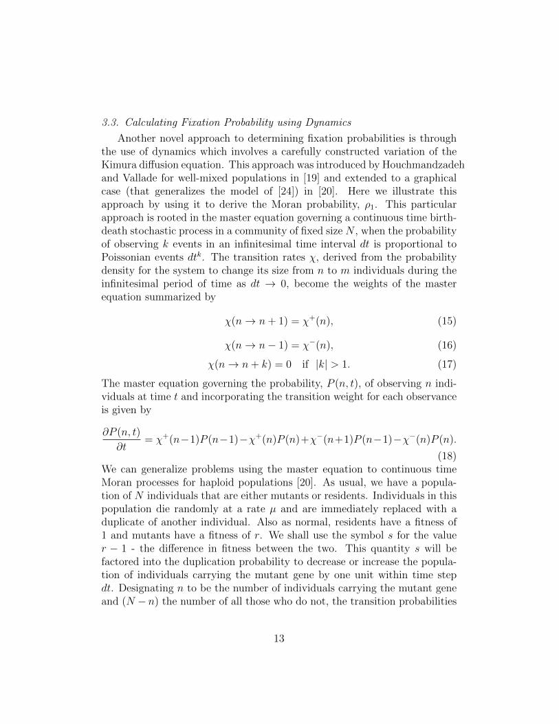
3.3. Calculating Fixation Probability using Dynamics

Another novel approach to determining fixation probabilities is throughthe use of dynamics which involves a carefully constructed variation of theKimura diffusion equation. This approach was introduced by Houchmandzadehand Vallade for well-mixed populations in [19] and extended to a graphicalcase (that generalizes the model of [24]) in [20]. Here we illustrate thisapproach by using it to derive the Moran probability, ρ1. This particularapproach is rooted in the master equation governing a continuous time birth-death stochastic process in a community of fixed size N , when the probabilityof observing k events in an infinitesimal time interval dt is proportional toPoissonian events dtk. The transition rates χ, derived from the probabilitydensity for the system to change its size from n to m individuals during theinfinitesimal period of time as dt → 0, become the weights of the masterequation summarized by

χ(n→ n+ 1) = χ+(n), (15)

χ(n→ n− 1) = χ−(n), (16)

χ(n→ n+ k) = 0 if |k| > 1. (17)

The master equation governing the probability, P (n, t), of observing n indi-viduals at time t and incorporating the transition weight for each observanceis given by

∂P (n, t)

∂t= χ+(n−1)P (n−1)−χ+(n)P (n)+χ−(n+1)P (n−1)−χ−(n)P (n).

(18)We can generalize problems using the master equation to continuous timeMoran processes for haploid populations [20]. As usual, we have a popula-tion of N individuals that are either mutants or residents. Individuals in thispopulation die randomly at a rate µ and are immediately replaced with aduplicate of another individual. Also as normal, residents have a fitness of1 and mutants have a fitness of r. We shall use the symbol s for the valuer − 1 - the difference in fitness between the two. This quantity s will befactored into the duplication probability to decrease or increase the popula-tion of individuals carrying the mutant gene by one unit within time stepdt. Designating n to be the number of individuals carrying the mutant geneand (N − n) the number of all those who do not, the transition probabilities

13

become [19]

χ−(n) = µn(N − n)

N(19)

χ+(n) = µn(N − n)

N(1 + r) (20)

where µn and µ(N −n) represent the probability per unit of time that eitherone mutant individual dies and is replaced by a resident individual or viceversa, respectively. The factor (1 + r) designates the differing fitness levelsof the mutants. Time will be measured in N/µ units so that µ/N = 1.

Because N and µ are fixed, equation 19 and equation 20 can be combinedas a function of two parameters allowing a slightly simpler version of equation18. Thus,

χ(n, s) = µn(N − n)

N(1 + r) (21)

and∂P (n, t)

∂t= α(n, r)P (n− 1)− β(n, r)P (n). (22)

where α(n, r) = χ(n − 1, r) + χ(n − 1, 0) and β(n, r) = χ(n, r) − χ(n, 0).To transform the discrete master equation 22 into a continuos differentialequation for large N , we must set x = n/N , dx = 1/N , p(x, t)dx = P (n, t),and ψ(x, r) = χ(n, r). Developing equation 22 by transforming each terminto powers of dx yields

∂p(x, t)

∂t= − 1

N

∂[α(x, r)p(x, t)]

∂x+

1

2N2

∂2[β(x, r)p(x, t)]

∂x2+O(dx3), (23)

and can be approximated by the Kimura diffusion equation, such that

∂p(x, t)

∂t= −Nr∂[x(1− x)p(x, t)]

∂x+∂2[x(1− x)p(x, t)]

∂x2. (24)

The neat thing about developing the equation this way is that we do nothave to use it as it is an approximation. By deriving Kimura’s diffusionequation using the applied transition rates we validate that the method issound. So instead of resorting to the approximation, we can take a moredirect route and extract exact quantities such as the probability generatingfunction (PGF) by letting

φ(z, t) =∑n

znP (n, t), (25)

14

where z is an auxiliary continuos variable. Notice that PGF φ(z, t) consti-tutes the most complete information we can have on the given stochasticprocess. The system will have two absorbing states at n = 0 and n = N .This will have the added effect of ensuring that φ(z, t) is a polynomial ofdegree N for n < 0 and n > N . Substituting φ(z, t) into the master equation22 yields

∂φ

∂t= 〈(zn+1 − zn)χ(n, r)〉+ 〈(zn−1 − zn)χ(n, 0)〉 (26)

We now turn to the transition rates, χ(n, r), for the Moran process. Recallthat because of the way we measure time, µ/N = 1 and therefore

χ(n, r) = k(r)n(N − n) (27)

where k(r) = 1 + r. Equation 26 becomes

∂φ

∂t= 〈(zn+1 − zn)k(r)n(N − n)〉+ 〈(zn−1 − zn)k(0)n(N − n)〉 (28)

We can now make use of the identity [19]

〈zn+αk(r)n(N − n)〉 = k(r)zαz∂

∂z

[Nφ− z∂φ

∂z

](29)

which when used to evaluate equation 28 yields

∂φ

∂t= (k(r)z2 − k(r)z + k(0)− k(0)z)

∂

∂z

[Nφ− z∂φ

∂z

](30)

= (1− z)(k(0)− k(r)z)∂

∂z

[Nφ− z∂φ

∂z

](31)

= (1− z)(k(0)− k(r)z)∂

∂z

[Nφ− z∂φ

∂z

](32)

=1

σ(1− z)(σ − z)

∂

∂z

[Nφ− z∂φ

∂z

](33)

where σ is the inverse of the fitness such that σ = k(0)/k(r) = 1/k(r) =1/(1 + r). This partial differential equation is well-defined and has the exactsame formal structure as the diffusion equation. Notice that it is first orderin time t and second order in z. The initial and boundary conditions arespecified as well. For the initial condition examine time t = 0. There are n0

15

individuals with the mutant gene. That means there is a 100% probability ofobserving n0 individuals have the mutant gene or P (n0, 0) = 1 and equation25 becomes

φ(z, 0) = zn0 . (34)

Further, because P (n, t) is stochastic we have a boundary in that

φ(1, t) = 1. (35)

If s = 0, then k(0) = k(r), 〈n(t)〉 = n0, and

∂φ

∂z

∣∣∣∣=1

= n0 if r = 0. (36)

If r 6= 0, z = σ is a fixed point because

∂φ

∂t

∣∣∣∣z=σ

= 0 if r 6= 0 (37)

which means thatφ(σ, t) = φ(σ, 0) = σn0 (38)

[20] demonstrate that equation 33 along with initial condition equation 34and the boundary conditions equation 35 with either equation 36 or equation38 constitute a well-posed problem.

Fortunately, φ(z, t) of equation 33 converges to stationary solution φs(z).This stationary solution is found by solving the first order differential equa-tion

Nφs(z)− zφ′

s(z) = K (39)

where K is a constant. The solution of 39 is

φs(z) = c1zN + c0 (40)

If we now use the boundary conditions 35 and 36 when r = 0, we can solvefor c1 and c0. They become

c1 =n0

N, c0 =

N − n0

N. (41)

Of course when r 6= 0, boundary condition 36 is replaced with 38 and

c1 =1− σn0

1− σN, c0 =

σn0 − σN

1− σN. (42)

16

It is interestingly to note that as r → 0, equation 42 converges to equation41. Note that for relatively small fitness, r, c1 of equation 42 contains thewell-known result for fixation probability for haploid populations, namely theMoran fixation probability result, equation 1 of the previous section.

ρ1 =1− 1/r

1− 1/rN(43)

4. Time to Fixation

In this section we explore an area of EGT that has recently seen someinteresitng activity: determining the mean time it takes to reach fixation.First we examine this for fixed values of r and then for the case where rdepends on the payoff of a two-player game.

4.1. Time to Fixation for Fixed Fitness

Here, we examine research on time to fixation when the fitness of the mu-tant and resident is fixed at r and 1 respectively (i.e., not determined by theoutcome of a game). In the undirected case, this was explored experimen-tally in [53], [10], and [42]. Generally, these studies find that certain graphstructures which promote fixation (i.e., stars and funnels) also increase timeto fixation. In [53], the authors find that stars increase the time to fixationover regular graphs by two orders of magnitude. In [42], the authors examinedomination times for lattices. Domination in that work refers to a mutant orresident occupying a large fraction of vertices (approaching N) - hence theterm ‘dominate’ is used to describe the results of [42] rather than fixation.They found experimentally that time t∗ for mutants to dominate lattices de-creases as the dimension of the lattice increases (i.e., a fully-connected graphhas a faster time to domination than a square lattice) for several differentvalues of r.

There has also been some work to explore this problem analytically. In[2], the authors provide a method for determining mean time to fixation (andmean time to extinction) in well-mixed populations. This formal method waslater adopted by [33] for fixed fitness and [7] for fitness resulting from a twoplayer game (described in the next section). We briefly highlight the mostrelevant parts of this method as follows. Given a well-mixed population of Nindividuals, let 0, . . . , i, . . . , N denote N + 1 possible states identified by thenumber of mutants in each state (analogous to the different configurations

17

in an evolutionary graph). We will use the notation Pi, Pi to denote fixationand extinction probabilities given initial state i. Let µi be the the transitionprobability from state i to state i − 1 and λi be the transition probabilityfrom state i to i+ 1. In [2], the authors show the following:

Pi =s0,i−1s0,N−1

(44)

Where sn,m =∑m

k=n qk and qi =∏i

j=1µjλj

. Now we define P(t)i , P

(t)i be the

probabilities of entering fixation/extinction at time t. Let ti (resp. ti) bethe mean times to fixation (resp. extinction) given state i at time 0. We areconcerned with finding t1 - the probability of fixation given a single mutantinvader. Clearly, Pi =

∑∞t=0 P

(t)i and we can obtain the following for the

mean time to fixation.

ti =1

Pi

∞∑t=0

t · P (t)i (45)

Additionally, the following recursions hold.

P(t)i = µiP

(t−1)i−1 + (1− µi − λi)P (t−1)

i + λiP(t−1)i+1 (46)

Piti = µiPi−1(ti−1 + 1) + (1− µi − λi)Pi(ti + 1) + λiPi+1(ti+1 + 1)(47)

Through a series of further manipulations and by expression 44, [2] determinethe mean time to fixation as follows.

t1 =N−1∑n=1

s0,n−1sn,N−1λnqns0,N−1

(48)

Note that [2] rely on determining mean time to fixation based on the transi-tion probabilities (for example, [2] look at when these fixation probabilitiesare dependent upon game-play, the problem becomes more complex, even forwell mixed populations). Further, in a well-mixed population there are N+1states, significantly less than the 2N possible states for an arbitrary evolu-tionary graph. Therefore, evolutionary graph theorists focus on reducing thestate space (usually by assuming a certain graph topology) and calculatingthe transition probabilities (µ and λ). If a certain graph topology allows fora tractable number of states, analytical results become apparent.

18

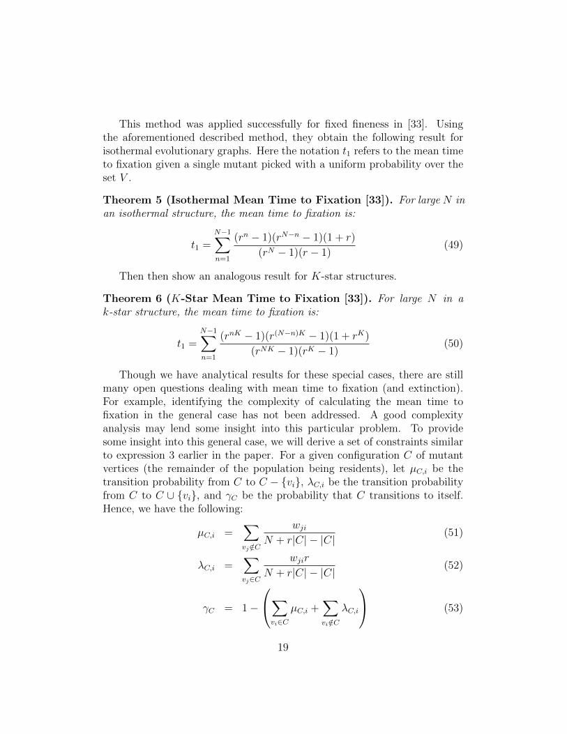
This method was applied successfully for fixed fineness in [33]. Usingthe aforementioned described method, they obtain the following result forisothermal evolutionary graphs. Here the notation t1 refers to the mean timeto fixation given a single mutant picked with a uniform probability over theset V .

Theorem 5 (Isothermal Mean Time to Fixation [33]). For large N inan isothermal structure, the mean time to fixation is:

t1 =N−1∑n=1

(rn − 1)(rN−n − 1)(1 + r)

(rN − 1)(r − 1)(49)

Then then show an analogous result for K-star structures.

Theorem 6 (K-Star Mean Time to Fixation [33]). For large N in ak-star structure, the mean time to fixation is:

t1 =N−1∑n=1

(rnK − 1)(r(N−n)K − 1)(1 + rK)

(rNK − 1)(rK − 1)(50)

Though we have analytical results for these special cases, there are stillmany open questions dealing with mean time to fixation (and extinction).For example, identifying the complexity of calculating the mean time tofixation in the general case has not been addressed. A good complexityanalysis may lend some insight into this particular problem. To providesome insight into this general case, we will derive a set of constraints similarto expression 3 earlier in the paper. For a given configuration C of mutantvertices (the remainder of the population being residents), let µC,i be thetransition probability from C to C − {vi}, λC,i be the transition probabilityfrom C to C ∪ {vi}, and γC be the probability that C transitions to itself.Hence, we have the following:

µC,i =∑vj /∈C

wjiN + r|C| − |C|

(51)

λC,i =∑vj∈C

wjir

N + r|C| − |C|(52)

γC = 1−

∑vi∈C

µC,i +∑vi /∈C

λC,i

(53)

19

We can now create an analogous recursion mirroring that of 46 for well-mixedpopulations where P

(t)C is the probability of entering an all-mutant state at

time t given initial set C.

P(t)C =

(∑vi∈C

µC,iP(t−1)C−{vi}

)+ γCP

(t−1)C +

∑vi /∈C

λC,iP(t−1)C∪{vi}

PCtC =

(∑vi∈C

µC,iPC−{vi}(tC−{vi} + 1)

)+ γCPC(tC + 1) +∑

vi /∈C

λC,iPC∪{vi}(tC∪{vi} + 1)

Clearly, as we are dealing with a intractable number of states there are anintractable number of constraints and variables the above expression, makingit impractical. Hence, a more practical algorithm is in order if we are to avoidsimulation for this problem.

Another option would be to explore mean time to fixation for specialcases, such as undirected evolutionary graphs or the case of neutral drift.Another area that is largely unexplored (in the general case) is time-to-fixation under alternate update rules, such as the voter model (although forgames on star graphs, we review the work of [15] in the next section).

4.2. Time to Fixation for Games on Graphs

Broom et al. [7] study evolutionary dynamics for general games on severalspecial graph structures: the star, the circle, and the complete graph under aBirth-Death update process (specifically the Invasion Process, see Section 5)while placing an emphasis on the speed of the evolutionary process in theiranalysis. At each time step, the fitness of an individual is assumed to bethe average of the payoffs of games against all its neighbors. The authorsanalyze and derive exact solutions for the fixation probability of mutants,the mean time to absorption and the fixation time of mutants on the threegraph structures considered. The authors find these quantities to differ forthe different graph structures and in general depend on population size andgraph heterogeneity.

The authors confirm earlier findings that fixation probability usually in-creases with graph heterogeneity. The time to fixation for mutants was found

20

to be shortest for the complete graph and longest for the star, confirming theresults from the previous section that fixation time generally is longer forgraph structures that promote fixation. Fixation times for all graphs ex-plored were also shown to be longest in neutral drift. More interestinglyhowever, using a Hawk-Dove game as an example, the authors show that thevariation of the payoff values in the payoff matrix of a game played on graphsplays a crucial role in the behavior of the analyzed quantities. Not only is thefixation probability no longer the same for all regular graphs with N vertices,but also which of the three considered graph types gives the highest mutantfixation probability and the fastest time to fixation/absorption depends onthe values of the game’s payoff matrix. The authors give several interestingfeatures of the Hawk-Dove game considered regarding the analyzed quanti-ties, but not that these results can be significantly different for a Hawk-Dovegame with an alternative payoff matrix.

In general, this work illuminates the fact that discovering and describing(to the extent that they exist) general and consistent patterns in the effects ofgame payoffs, graph types, and combinations thereof on fixation probabilityand time to fixation is a challenging but important area for future work. Had-jichrysanthou et al. [15] make a step of progress in this direction by providinggeneral formulae for fixation probability and mean time to absorption for stargraphs specifically. The authors provide detailed analysis of these quantitiesfor the fixed fitness case and the Hawk-Dove, Prisoner’s Dilemma and coor-dination games. They find that the time to absorption on star graphs dependcrucially on the update process used: while in general Birth-Death processesyield higher fixation probabilities for advantageous mutants, Birth-Deathprocesses take much longer to reach fixation/absorption than Death-Birthprocesses (see Section 5 for details on these update processes). There is stillmuch room for this type of work on more general graphs:

Open Problem 4.1. Discover and describe patterns of the effects of a largervariety of graph structures, game payoffs, and their combinations on fixationprobability and time to fixation.

5. Alternate Update Rules

Let us momentarily return to the original model of [23]. At each time-step,some vertex vi is selected with probability fi∑

vj∈V fj, where fi is the fitness of

vi and equal to either 1 or r. This is the vertex chosen to reproduce, hence a

21

Table 1: Different families of update rules.

Update Rule Intuition

Birth-Death (BD) (1) vetex vi selected(a.k.a. Invasion Process (IP)) (2) Neighbour of vi, vetex vj selected

(3) Offspring of vi replaces vjDeath-Birth (DB) (1) vetex vi selected(a.k.a. Voter Model (VM)) (2) Neighbour of vi, vetex vj selected

(3) Offspring of vj replaces viLink Dynamics (LD) (1) Edge (vi, vj) selected

(2) The offspring of one vetex in theedge replaces the other vetex

‘birth’ event. The next vertex selected is one of the neighbors of vi - lets callit vj and it is selected with probability wij. This is a ‘death’ event as vj isreplaced with a duplicate of vi. Notice that the fitness of vj is not consideredwhen it is selected. Hence, the fitness bias is on the birth event. This methodof selecting vertices vi and vj is referred to as an update rule. The update ruledescribed in [23] is termed ‘birth-death with birth bias’ or BD-B updating.Several works address different update rules including: [1, 38, 47, 26, 25].Overall, we have identified three major families of update rules - birth-death(a.k.a. the invasion process) where the vetex to reproduce is chosen first,death-birth (a.k.a. the voter model) where the vetex to die is chosen first,and link dynamics, where an edge is chosen. We summarize these in table 1.

Note that the three categories of table 1 are very broad as they do notconsider fitness-based bias in vetex selection (i.e., the BD-B updating of [23]places the bias on the birth event as the first vertex is chosen with a prob-ability proportional to its fitness). If there is a birth-bias, the individualreproducing is chosen with a probability proportional to its fitness. If thereis a death-bias, the individual dying is chosen with a probability inverselyproportional to its fitness. We summarize how directionality and bias affectthe update rules in table 2. Note that imitation (IM) is also known as biasedlink dynamics.

22

Table 2: Variations of EGT. vi and vj are vertices in a graph that are neighbors, vi isalways chosen first. fi and fj are the associated fitness values which both equal 1 in thecase of neutral drift.

Update Rule Special Case Intuition

Birth-Death (BD)

Unbiased, undirected offspring of vi replace vjDirected Considers vi’s outgoing edgesBiased-birth (BD-B) vi chosen w. prob. proportional to fiBiased-death (BD-D) vj chosen w. prob. proportional to f−1j

Death-Birth (DB)

Unbiased, undirected offspring of vj replace viDirected Considers vi’s incoming edgesBiased-birth (DB-B) vj chosen w. prob. proportional to fjBiased-death (DB-D) vi chosen w. prob. proportional to f−1i

Link Dyn. (LD)

Unbiased, undirected one vetex reproduces to replace the otherImitation (IM) least fit vetex dies, replaced by offspring

of other vetexPairwise Compar. (PC) vj replaces vi iff fj > fx, o/w no changeDirected, unbiased edge from vi to vj, vi replaces vjDirected, birth biased edge selected w. prob. proportional to fiDirected, death biased edge selected w. prob. proportional to f−1j

23

Table 3: Relationship between fixation and degree of initial vetex (undirected graphs).

Update Rule Fixation probability proportional to

BD-B Inverse of degree of initial vetexDB-D Degree of initial vetexLD Density of mutant vertices

5.1. Comparing Update Rules in Undirected EG’s

For the case on undirected graphs, there are many results based on theinitial placement of the mutant have been discovered for several update rules(as we have described for BD-B in the previous section). In [1, 47], theauthors study moments of degree distribution, density, and degree-weightedmoments and show that the fixation probability is proportional to the averagedegree-weighted moment for death-birth updating (a.k.a. voter model), theinverse for birth-death (a.k.a. invasion process), and equal to the density(the percentage of the number of vertices in the graph labeled as mutants)for link dynamics, thus independent of the underlying graph in that case.Note that their results for BD-B are in agreement with the finding of [10]described earlier.

As shown in theorem 4, under BD-B, an undirected EG is isothermal iffit is regular. In [1], this is extended to other update rules as follows.

Theorem 7 ([1]). Evolutionary dynamics under BD-B, DB-D, and LD areequivalent for undirected regular EG’s.

Although there is currently an excellent suit of results for studying evolu-tionary graphs under various different update rules in the directed case, therehas been no work (to the knowledge of the authors) that compares any ofthese update rules to the synchronous update model described by Santos etal. in [44].2 At each time-step, all individuals in the population update theirlabels (i.e., mutant or resident, or strategy if game-play is involved) simulta-neously. For each vertex vi, one of its neighbors (vertex vj) is selected at 1

di.

2Note that the original work of Santos et al. is a model with a game theoretic extension.Here we describe the natural, fixed fitness counterpart for the purpose of examining theupdate rule. We review this work with respect to its game theoretic results in Section 6.

24

Then, if and only if fj > fi, vi’s label is replaced with vj’s label with a prob-

ability proportional to fj−fi (i.e.,fj−fi

max(di,dj)·r for example). There are several

interesting aspects about this model. For instance, the fitness of vertices doesnot play a role in selecting which vertex is born and/or dies. Rather, thefitness determines if a vertex is replaced by a neighbor and the probability atwhich this happens. Additionally, as all vertices are updated simultaneously,we might conjecture that the evolutionary process occurs faster than in theother update rules. These topics may warrant some further consideration inthat synchronous updates may represent some real-world processes more ac-curately or possibly be used as a proxy for the standard update rules we havealready described. Further, the synchronous update model can also easily beextended to the directed case, which we cover for the other update rules inthe next section.

5.2. Comparing Update Rules in Directed EG’s

Not only does the original model of [23] utilize a directed graph, but manyreal-world networks can be more accurately modeled as directed graphs thanundirected ones. This is the motivation of the work [26, 25]. There are twomain conclusions to their work: (1) degree correlation to fixation probability(i.e., using the exact methods of [8] or the mean-field approximation) forundirected graphs does not necessarily hold in the direct case and (2) directedgraphs generally suppress fixation more than undirected ones.

In [26], the authors study directed graphs under LD, BD, and DB for r = 1.For all three update rules, under r = 1, they derive sets of linear constraintsusing the mean-field approximation (degrees of connected vertices in theEG are uncorrelated). They compare these analytical approximations withexperiments and find that, in general, the fixation probability is not onlydependent on the degree of the initial vetex but also the global structureof the graph. In fact, often there is no observed relation between degreeand fixation. See table 4 for a summary of experimental results comparedwith the analytical approximations. While [26] mainly considers the case ofneutral drift (r = 1), they also run some tests with r = 4 and claim thatfixation increases monotonically with r.

In [25], the authors perform an in-depth comparison on directed andundirected networks for several variants of these rules. He exactly computesfixation probabilities on an exhaustive set of small graphs (with six vertices)and uses Monte-Carlo approximation for randomly generated larger graphs.He found that directed networks tended to suppress more than undirected,

25

Table 4: Summary of experimental results for directed case with r = 1 in [26] illustrat-ing whether experimentally-determined fixation probability results that alighned with themean-field approximation. din and dout are the in and out degrees of the initial mutantvetex.

Mean-field approximation BD: 1/din DB: dout LD: dout/din

Asymmetric random 1/din dout dout/dinAsymmetric scale-free No relation dout dout/dinE-mail No relation No relation No relationAsymmetric Small World No relation No relation No relation

regardless of update rule. Based on these experiments for small networks, theorder of amplification for rules is as follows: BD-B > LD > DB-D > BD-D >DB-B (BD-B was least suppressive and DB-B was the most suppressive). Thevalue of r was set to 4 in these trials. For large graphs (also with r = 4), thesimulations provided the following ordering: BD-B > BD-D, LD > DB-D >DB-B.

The authors are currently looking at adopting the algorithm of [45] foralternate update rules on directed EG’s, which would allow us to obtain moreexact and deterministic results on larger graphs(as we would not resort tosimulation). This would provide a complement to the work of [25].

6. Further Game Theoretic Extensions

Now that we have described alternate update rules, we shall re-visit ourgame-theoretic extensions and review some results regarding topics such ascooperation, reciprocity, and evolutionary stability w.r.t. a game on thegraph under various update rules.

6.1. Evolutionary Stability on Graphs

Evolutionary stability, describing the ability of a player type comprisinga population to be resistant against invasion by another type, is an impor-tant concept in evolutionary game theory that has been well studied forwell-mixed populations. Ohtsuki et al. [40] analyze evolutionary stabilityon regular graphs of degree k > 2 for the BD, DB, and IM updating rulesthrough pairwise approximation and simulation. Evolutionary stability ongraphs means that a small fraction of rare mutants cannot spread, i.e., a

26

resident strategy evolutionarily stable if it has a selective advantage over aninvading strategy (invading at an ε fraction of the total population). Oht-suki et al. provide evolutionary stability conditions for this definition onregular graphs for the different update rules considered, and (on top of thegame payoff matrix values) all these conditions depend on the graph degreek. The results are validated through simulations on specific game examples.The important point to consider from these results is that population struc-ture can have crucial impact on the evolutionary stability of strategies, i.e.,in the words of “traditional criterion for evolutionarily stable strategies inwell-mixed populations is neither necessary nor sufficient to guarantee evo-lutionary stability in structured populations”.

6.2. Regular Graphs and the Replicator Equation

Ohtsuki et al. [38] study evolutionary games on regular graphs of degreek considering the BD, DB, IM, PC update rules3. The authors use pair ap-proximation ([28, 27, 22, 17, 51]) to derive a system of ordinary differentialequations describing the change in expected frequency of strategies in a gameon a graph over time. In the limit of weak selection (w << 1), the authorsshow that under the update rules BD, DB, and IM this differential equationis the well-known replicator equation with a transformed payoff matrix. Thepayoff matrix is the original payoff matrix summed with a payoff matrix de-scribing the local competition of strategies, different for BD, DB, and IM. PCis shown to be equivalent to BD in the model used. This result is applied tothe Prisoner’s Dillema and the Snow Drift Game on regular graphs. Resultsfor the Prisoner’s Dillema coincide with those of [36], showing identical con-ditions necessary for cooperators to be favored over defectors. Results forthe snow drift game qualitatively agree with those of Hauert et al. [18], whoobserve that spatial structure inhibits cooperation in the snow drift game.

6.3. Evolution of Cooperation and Social Viscosity

Ohtsuki et al. [36] explore the problem of cooperation on a variety ofgraphs through numerical simulations. The graph types explored are cycles,spatial lattices, random regular graphs, random graphs and scale free net-works. Every player plays a game with all its neighbor, where the game

3We use the shorter BD and DB notation for the update rules with birth bias BD-Band DB-B. See Table 2.

27

between two players is given by the payoff matrix (54) below. This gamerepresents a Prisoner’s Dilemma game between two players, and gives a kindof Public Goods Game when each player plays the game with all its neigh-bors. In this game b is called the benefit of the altruistic act and c is thecost of the altruistic cooperation act. A Cooperator that is connected to nCooperators and m Defectors for receives a payoff of b n− c (n+m).

cooperate defectcooperate b - c - c

defect b 0(54)

Ohtsuki et al.’s results suggests that under the DB update rule, a neces-sary condition for cooperation to arise in the types of graphs explores is thatb/c > k, where k is the average number of neighbors. This result is derivedunder the conditions of weak selection and that the number of vertices in thegraph is much larger than the average degree. The authors note the closeand interesting relation of this result to Hamilton’s rule ([16]), which statesthat kin selection can favor cooperation provided that b/c > 1/r, where r isthe coefficient of genetic relatedness between individuals. The condition forcooperation fits less well for non-regular graphs, as one would expect due tothe larger variance in vertex degrees, but is a good approximation unless thevariance in degree distributions of the graph gets too large. Other dynamicsexplored are IM 4, for which cooperation is favored when b/c > k + 2, andBD, for which cooperation is never favored by selection.

Other authors have verified the condition introduced in [36] to hold in adifferent model with network dynamics. Yang et al. [12] use pair approxima-tion and numerical simulations to deduce cooperation frequencies for socialdilemma games (including the Prisoner’s Dilemma and Snow-Drift games) ongraphs whose structure changes as part of the update rule throughout evolu-tion. The graphs originally are randomly connected with average degree k.The update rule used is a type of DB process which also involves additionand deletion of vertices and edges in the graph: “An individual is selectedfor reproduction with a probability proportional to his fitness. The offspring

4The authors of [36] also note that mathematically, “IM updating can be obtainedfrom DB updating by adding loops to every vertex”.

28

is introduced with the same strategy of his parent and connects to his parentalways and other k − 1 individuals randomly. The offspring replaces a ran-dom individual except for his parent. The randomly selected individual withall its links are removed.” More recently, the preliminary work of Zhong etal. [57] also confirmed Ohtsuki’s rule on a continuous version of the model.

In [52], Voelkl and Kasper used evolutionary graph theory to understandthe emergence of cooperation in primates. Using social interaction networksderived from empirically observed social interactions, they looked at a twoplayer game with payoff matrix as above (54). The authors use selectionintensity equation 4 with w = 0.01 to determine fitness. The authors dis-covered that the structured populations of the primates were more likely toreach fixation than populations of well-mixed individuals.

The authors of [52] also looked at the community structure of the pri-mate interaction networks. For this they leveraged the idea of modularityintroduced in [31]. Given a partition of vertices in a graph, modularity mea-sures the quality of these partitions - often referred to as “communities”.Intuitively, the modularity of a partition increases with the density of edgeswithin communities and decreases with the density of edges outside of com-munities. Often in work dealing with modularity (such as [30] and [5]) re-searchers attempt to find an optimal partition. Hence, the modularity of theoptimal partition can also be viewed as a property of graph topology. Theauthors of [52] compare optimal modularity values to fixation probability(ρ, determined by simulation) using linear regression. This led them to theconclusion that 60% of the variance in fixation probability can be accountedfor by the modularity of the graph. An interesting direction for future workwould be a more detailed examination on the relationship between ρ andoptimal modularity based on a wider variety of graphs.

6.4. Graph Heterogeneity and Evolution of Cooperation

Santos et al. [44] investigate the effects of single-scale and scale-free net-works on cooperation in the Prisoner’s Dillema, Snow-Drift, and Stag-Huntgames through simulations. The update rule used is a type of imitationdynamic in which all vertices update simultaneously in each generation, asfollows: for each vertex a random neighbor is chosen, and if that neighborhas achieved a higher payoff, the vertex adopts the strategy of this neighborwith a probability proportional to the payoff difference. The authors findthat in degree-heterogeneous graphs cooperation is easier to sustain than in

29

well-mixed populations and thus identify heterogeneity as a “powerful mech-anism for the emergence of cooperation.” Additionally, the authors find thatthe sustainability of cooperation also depends on“detailed and intricate ties”between agents. As evidence of this, scale free networks which exhibit prop-erties like those that emerge from models of growth from preferential attach-ment (Albert-Barbarasi topology) are shown to produce higher cooperationthan random scale-free networks.

Fu et al. [13] devise a framework for the general study of games on ar-bitrary graphs under weak selection, formulating the game dynamics as adiscrete Markov process. Using DB updating and the game of the prisoner’sdilemma, they employ their method on random regular graphs and scale-free networks to demonstrate the utility of their framework compared topair-approximation and simulated data. The authors find a stronger corre-lation between their approach and the simulated results. They also reachsome conclusions on the evolution of cooperation, most notably that underDB updating and weak selection, degree heterogeneous graphs (e.g., scale-free networks) generally impose higher invasion barriers than regular graphs.This extends a result in [1] reporting that a heterogeneous graph is an inhos-pitable environment for a mutant to evolve in the case of constant selection.Fu et al. show this to be true for weak selection as well. This result seems tobe in disagreement with the conclusion of [44], which concludes that graphheterogeneity aids the emergence of cooperation. Fu et al. point out thatthis conclusion by [44] hinges on the simultaneous appearance of a numberof cooperators to overcome the invasion barrier.

6.5. Direct Reciprocity on Regular Graphs

Ohtsuki et al. [37] study reciprocity in the iterated prisoner’s dilemma(exhibited by strategies such as Tit-for-Tat) on large, regular graphs throughpair approximation for the four update rules BD, DB, IM, and PC underweak selection. The game concerned is again that of payoff matrix (54), buttranslating the payoffs in the matrix to a repeated game with q probability ofplaying another iteration and assuming a game between reciprocators playingTit-for-Tat and Defectors All-D gives the following payoffs:

cooperate defectcooperate (b− c)/(1− q) - c

defect b 0(55)

30

The authors are particularly concerned with evolutionary stability and“advantageousness” of reciprocators and find that different update rules havea critical effect on these measures. A strategy is termed “advantageous” ifa single mutant following the strategy starting in a random position on thegraph has a fixation probability greater than the inverse of the populationsize, meaning that selection favors it over residents. The authors find thatthe ratio b/c necessary for a cooperator to be advantageous depends onlyon the probability to play another round in the repeated game (q) and thenumber of neighbors per individual (k). BD and PC produce identical results,showing evolutionary stability to be harder to achieve for cooperators ongraphs compared to well-mixed populations, but it is easier for cooperationto be advantageous. In contrast, DB and IM updating make it easier forcooperation to be both evolutionarily stable and advantageous. In particular,for DB and IM either small k or large q are sufficient for the evolution ofcooperation.

6.6. Separate Interaction and Replacement Graphs

Ohtsuki et al. [39] examine the evolution of cooperation in games on reg-ular graphs - again with payoff matrix (54) . However, unlike other work,the graph for the interactions between players in the game (interaction graphH), and the graph among the relationships of who can replace whom (re-placement graph G) are separate. The authors consider the case of weakselection, where w << 1. The authors use BD, DB, and IM updating. Theauthors consider regular graphs and again use pair approximation for theiranalysis of fixation probabilites. For DB updating, the authors find the fol-lowing result, which is verified through experiments: if c and b are the costand benefit associated with the game, ` is the degree of overlap between Gand H, and g and h are the degrees of G and H, then the following in-equality holds under death-birth updating: b/c > hg/`. Hence, the authorsconclude that, for fixed cost and benefit values, cooperation is less likely toevolve if there is a greater disparity between the interaction and replacementgraph, cooperation is maximized when G and H coincide. IM updating leadsto b/c > h(g + 2)/`, while BD, as has been shown before, never gives anevolutionary advantage to cooperators.

6.7. Further Work for Game Theoretic Extensions

A main area for future work is the extension of any of the results asdescribed in this section to games with more than two competing strategies

31

on graphs, as well as for multi-player (> 2) games:

Open Problem 6.1. Extend results on evolutionary games on graphs topopulations with more than two competing strategies and multi-player games.

However, there are still a significant amount of issues to explored in two-player games. As noted in [35] the benefit-cost payoff matrix (54) usedin a number of works described is only a simplified version of the generalPrisoner’s Dilemma game that has been so important in the study of theevolution of cooperation. Extending results to the general game seems to beof considerable importance to the study of the evolution of cooperation ongraphs:

Open Problem 6.2. Extend results that used the benefit-cost payoff matrix(54) version of the Prisoner’s Dilemma to the general Prisoner’s Dilemmagame payoff matrix.

In reviewing work on games in EGT, we have noted and important differ-ence in fitness assignment used by different researchers, the effects of whichare unclear: While some works have used the average payoff of games ongraphs in their fitness computation and resulting analysis (e.g., Broom et al.[7]) others use the total accumulated payoff of games. (e.g., Ohstuski et al.[36] and Santos et al. [44]). There is an important distinction between theseon heterogeneous graphs: the former excludes the effect of playing a differentamounts of games due to different amounts of neighbors, while the latter doesnot. It’s important to be aware of this difference and it’s of high interest tothe community to explore to what extent analytical and experimental resultsare affected by this difference.

Open Problem 6.3. Explore and understand the effects of using the aver-age vs. accumulated payoff from games played with neighbors for fitness inevolutionary games on graphs.

On the analysis of reciprocity, while Ohtsuki et al. [37] have considereddirect reciprocity in their analyses for regular graphs, as noted by Nowak etal. [35], much more work is needed to work direct and indirect reciprocityinto the mathematical frameworks presented by different authors (or a gen-eral one) encompassing various update rules and more complex populationstructures:

32

Open Problem 6.4. Incorporate direct and indirect reciprocity into a gen-eral mathematical framework for evolutionary games on graphs.

Concerning punishment and reputation, past work on spatial evolution-ary games (e.g., [6]), where the population is structured on a simple grid,has explored the effects of punishment and reputation on the evolution ofcooperation. However, the exploration of these mechanisms on general andcomplex population structures has not yet been explored:

Open Problem 6.5. Using EGT to explore the effects of punishment andreputation on the evolution of cooperation under the constraints of general,more complex, population structures.

Generally, we feel there exists a need to incorporate EGT into more evolu-tionary game theory applications: many existing applications of evolutionarygame theory, particularly those in anthropology, economics, and social mod-eling and prediction could possibly greatly from EGT by using it to accountfor effects of population structure.

Open Problem 6.6. Incorporate known or estimated population structuresinto more existing evolutionary game theoretic applications.

7. Other Extensions to the Model

There are several other notable extensions to the original model of [23]worth noting. These include scenarios with bi-level graphs, multiple mutants,EG’s whose topology changes over time, and other modifications.

7.1. Bi-Level Evolutionary Graphs

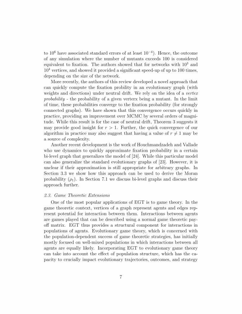
Pu Yan Nie introduces bi-level EG’s in [32]. In general, a bi-level EG isdefined as follows: first, there is an EG representing relationships betweencommunities - with the vertices in this graph representing communities. Thework on bi-level EG’s often denote the community-level EG as graph B. Eachof the m vertices of B is itself an EG of individuals - vertex vi on graph B isEG Ai. This type of EG has been shown to help describe several biologicalphenomena. In the bi-level EG’s of [32, 56], one of the vertices in graph B isan isothermal EG consisting of n individuals (‘leaders’). The remaining m−1vertices in graph B represent single individuals (‘followers’). Hence, for theentire graph, N = n + m − 1. As only one vertex in graph B represents an

33

A

Figure 2: A bi-level EG where the leaders (set A) form an isothermal EG. When they arecollapsed into a single vetex, we have a one-rooted EG.

EG, these works use A to refer to the EG consisting of the n leaders. As thestructure of A and B are independent, we have the following relationship:

ρ(AB) = ρ(A) · ρ(B) (56)

where ρ(AB) is the fixation probability of the entire bi-level EG, and ρ(A), ρ(B)are the fixation probabilities of EG’s A and B respectively. In [32], graph Bis a star formation (K = 2,M = 1), with the central vetex being equivalentto EG A. The author shows that for r 6= 1 this bi-level graph suppresses fixa-tion more than an isothermal graph, thus helping to explain the evolutionarystability of bi-level structures found in nature. In [56], the authors study abi-level EG where B is one-rooted and A is equivalent to the root-vetex ofB (see figure 2). The one-rooted case reflects hierarchical population struc-tures. The authors show that when the number of followers is identical, thata bi-level EG has a lower fixation probability than a one-rooted EG. Theyalso show that the fixation probability increases when the number of leadersincrease (making a bi-level EG of this type with 2 leaders the most stable bi-level EG). They also show that an increase in number of followers decreasesfixation probability and that fixation probability for a bi-level EG is closelytied to fitness. The authors apply these theoretical results to biology to helpexplain why structure occurs in some animal populations. Examples of thisinclude symbiosis (such as the growth of Lichens) and commensalism (i.e.,the relationship between clownfish and sea anemone).

The work on bi-level EG’s is extended in [55] where the authors considerbi-level EG’s where the mutant has a different fitness depending on the levelof the graph. The model is described as follows. In this work, each vertexof B is associated with an EG. Hence, vertices v1, . . . , vi, . . . , vm in EG Bare associated with EG’s A1, . . . , Ai, . . . , Am. Each of these groups has ni

34

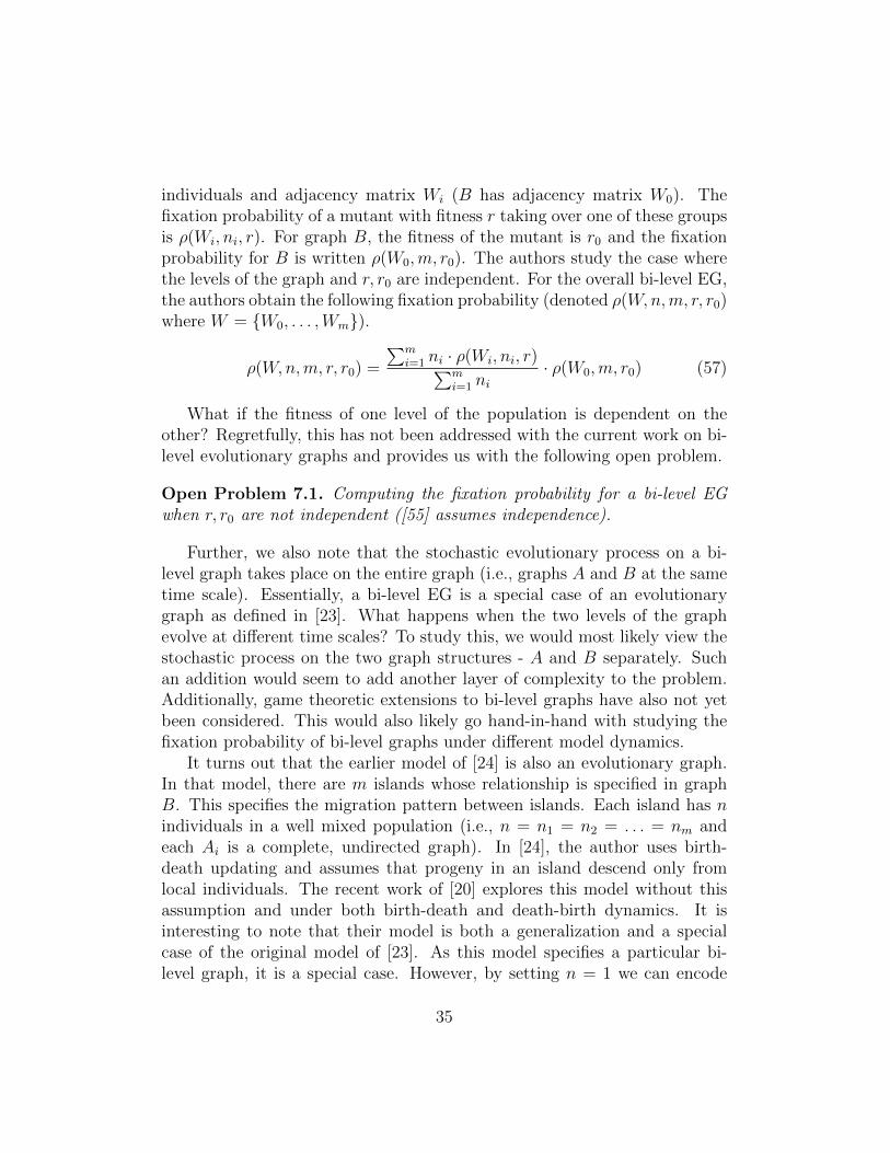
individuals and adjacency matrix Wi (B has adjacency matrix W0). Thefixation probability of a mutant with fitness r taking over one of these groupsis ρ(Wi, ni, r). For graph B, the fitness of the mutant is r0 and the fixationprobability for B is written ρ(W0,m, r0). The authors study the case wherethe levels of the graph and r, r0 are independent. For the overall bi-level EG,the authors obtain the following fixation probability (denoted ρ(W,n,m, r, r0)where W = {W0, . . . ,Wm}).

ρ(W,n,m, r, r0) =

∑mi=1 ni · ρ(Wi, ni, r)∑m

i=1 ni· ρ(W0,m, r0) (57)

What if the fitness of one level of the population is dependent on theother? Regretfully, this has not been addressed with the current work on bi-level evolutionary graphs and provides us with the following open problem.

Open Problem 7.1. Computing the fixation probability for a bi-level EGwhen r, r0 are not independent ([55] assumes independence).

Further, we also note that the stochastic evolutionary process on a bi-level graph takes place on the entire graph (i.e., graphs A and B at the sametime scale). Essentially, a bi-level EG is a special case of an evolutionarygraph as defined in [23]. What happens when the two levels of the graphevolve at different time scales? To study this, we would most likely view thestochastic process on the two graph structures - A and B separately. Suchan addition would seem to add another layer of complexity to the problem.Additionally, game theoretic extensions to bi-level graphs have also not yetbeen considered. This would also likely go hand-in-hand with studying thefixation probability of bi-level graphs under different model dynamics.

It turns out that the earlier model of [24] is also an evolutionary graph.In that model, there are m islands whose relationship is specified in graphB. This specifies the migration pattern between islands. Each island has nindividuals in a well mixed population (i.e., n = n1 = n2 = . . . = nm andeach Ai is a complete, undirected graph). In [24], the author uses birth-death updating and assumes that progeny in an island descend only fromlocal individuals. The recent work of [20] explores this model without thisassumption and under both birth-death and death-birth dynamics. It isinteresting to note that their model is both a generalization and a specialcase of the original model of [23]. As this model specifies a particular bi-level graph, it is a special case. However, by setting n = 1 we can encode

35

an arbitrary evolutionary graph. Adopting the technique of [19] for well-mixed populations, (see Section 3.3) the authors develop an approximationtechnique for fixation probability under this model. For r > 1, they showthat the approximation is valid when n ·m · (r− 1) is approximately greaterthan 1. However, it is unclear how this approach can scale, particularly asm increases - all of the experiments in [20] had m ≤ 5 (the experimentswhere the approximation performed the best had n = 50). Not only is thescalability of this approach an area for future work, but the issue of thetopology of the Ai graphs as well. Can the same approach be used for anarbitrary bi-level graph?

In [55], the authors describe several anecdotal applications of bi-levelEG’s. or example, describe several species whose populations resemble anon-hierarchical bi-level EG where both upper and lower level structures areisothermal including the budgerigar of Oceania and the aptenodytes fosteri(emperor penguins) of Antarctica. However, in [58] the authors take a stepfurther toward a real-world application by using bi-level EG’s and star EG’sto examine the stability of various types of business forms. Specifically,they look at corporations with individual decisions (CID’s), multi-persondecision corporations (MDC’s), and stock corporations (SC’s). They modelCID’s as 1-level star graphs and MDC’s and SC’s are modeled as bi-levelgraphs. They find that, under reasonable conditions, MDC’s have a higherfixation probability than CID’s, which have a higher fixation probability thanSC’s. Hence, by through the lens of EGT, SC’s represent the most stableorganizational structure for business.

7.2. Multiple Mutants

In [41], the authors discuss the issue of clonal interference where twodifferent lineages in a population compete with each other. In such a case,multiple mutations exist in a population. Hence, the authors of this workextend the model of [23] to allow for this case. These mutants are referredto as type-1 and type-2 mutants. The authors are primarily concerned withdetermining the fixation probability of the type-2 mutants. The authors viewthe population of individuals as two disjoint sets. The first set defined bythe authors is the set of type-1 mutants which is referred to as the residentmutant population (RMP). The authors use use m1 to denote the cardinalityof this set. The second set is the set of residents in the population which arereferred to as the wild type population (WTP). There are N −m1 individualsin this set. To obtain the fixation probability of the type-2 mutant (ρ(2)),

36

the authors consider the fixation probability of the type-2 mutants within theWTP and RMP populations. As the probability that a type-2 mutant occursin the WTP and RMP populations are (N −m1)/N , m1/N respectively, theauthors derive the following equation for the fixation probability of the type-2mutant:

ρ(2) =(N −m1) · ρ(2)WTP

N+m1 · ρ(2)RMP

N(58)

where ρ(2)WTP is the fixation probability of a type-2 mutant in the WTP

and ρ(2)RMP is the fixation probability of the type-2 mutant in the RMP. The

authors come up with analytical approximations of fixation probabilities forthe type-2 mutants in the cases of lines and fully-connected graphs. Theseapproximations work well in the cases where m1 >> 1 and r is high. For a

lines, they obtain m1·(1−1/r)N

+ (N−m1)2

2·N2 · (1 − 1/r) and for a fully-connected

graph they obtain N−m1

N· 1m1+1

+ m1

N·(

1− N+(r−1)m1

Nr2

)The authors perform

simulation experiments that aligned well with these analytical results. Hence,they were able to demonstrate that topology and the population of the type-1 mutants figures significantly into fixation probability calculations in realpopulations.

7.3. EG’s that Change Over Time

In [3], the authors modify the original formulation of [23] by examin-ing a simple class of graphs that change over time [3]. Specifically, theylook at layered networks. They find, through experimental simulation, thattheir growth structure also substantially increases the fixation probability.In future work, the authors intend to explore a more general framework fordynamic graphs.

In [10], the authors conjecture results for undirected graphs that changeover time for BD-B. They conjecture that existing BD-B results still hold ifthe graph changes more slowly than it evolves. They also suspect that even ifthe graph does not change slowly, that existing BD-B results will still provide‘good’ estimates.

Overall, studying fixation probability on a graph whose topology changesover time is an area ripe for new research. For example, preferential at-tachment has been observed in graph-structured with evolving topologiesand essentially states that vertices of high degree are more likely to increase

37

their connections as time progresses [21]. Now consider birth-death updat-ing, where the results described in the previous sections show that fixationprobability is inversely proportional to its degree. So, under preferential at-tachment with birth-death updating, do new mutant vertices whose degreeincreases end up suppressing evolution as they connect to more residents?How do the time scales of the topology evolution with the evolution of themutant trait affect each other? Further, would alternate methods of graphevolution, such as the biologically-inspired models of [48] affect fixation (i.e.,as compared to preferential attachment)?

7.4. Further Extensions

In [42], the authors examine the model of [23] under birth-death updatingon graphs where vetex connectivity is fixed - specifically lines, square lattices,cubic lattices, and fully-connected graphs. They then extend the model toallow offspring to not be perfect clones of their parents. Further, in theirmodel, the offspring of a parent subject to a mutation with a probability ofµ and increase the fitness with a probability p, or decrease it with probability1− p. The calculation of the new fitness for the offspring is based on a pre-viously studied model. They examined their asexual model experimentallyon graphs with 250, 000 vertices and the results showed that the equilibriumfitness of the population was correlated with the dimensionality of the lattice- specifically that more connected graphs had a higher level of equilibriumfitness. No saturation was observed for the fully connected graph in thiscase. The authors also examined a modification to the model allowing forsexual reproduction with multiple genes per vetex. For sexual reproduction,the equilibrium fitness increased not only with the dimension of the lattice,but also with the population.

In [54], the authors study EGT in the case where the fitness of the mutantchanges with its frequency. For example, the fitness of cancer cells changeswith frequency which often causes a failure in therapy. Given a population ofsize N , they assume N different values of r – each associated with a differentnumber of mutants in the population. They assume r1 ≤ r2 ≤ . . . ≤ rN andobtain analytical approximation for the fixation probabilities of super-starsand isothermal EG’s.

In [53], the authors consider a ‘local’ version of the Moran process wherethe update rules are dependent upon a deme. In this work, a deme (indexedthe same way as the vertices in v) corresponds to the neighborhood of agiven vertex. In this case, [53] adds the requirement that for each vetex vi,

38

wii > 0 (note that this type of self-loop is not permitted in the original modeof [23]). At each step, a row Wi of the matrix is chosen with a probability1/N . Next, a vetex vj is selected s proportional to the fitness of all vertices inthe deme. Finally, the vetex to be replaced is selected based on the outgoingedge weights of vj. The authors experiment with this process on star andKawachi-style small world networks to find that this process achieves theMoran probability for fixation.

8. Conclusion

In this paper we have described evolutionary graph theory, which wasfirst introduced in [23] and generalizes the classic Moran process of [29]. Wehave described the original model, the major results and extensions, andapplications to game theory. While this is still a relatively new tool for fieldssuch as biology, physics, game theory, and computer science, the number ofpublications on the topic seems to be steadily increasing each year - henceresulting in this review. Our view is that there is great potential with EGTfor a variety of applications, and that represents the next wave of research inthis area. Applied work such as [58] for economics and [52] in biology mostlikely represent just the beginning of a new trend. However as EGT becomesmore operational, many new questions arise. First, how can the model beadjusted for certain applications? Second, can we learn the model and/ormutant fitness from historical data? Third, many real-world applicationsutilize large data sets, for example, a data set LiveJournal social networkdata set consists of over 4 million vertices and over 6 million edges.5 Canprocedures for calculating fixation probability and time to fixation be scaledfor these large data-sets? There are multiple directions in which EGT can betaken. We are very excited about the possibilities due to the large problem-space.

Acknowledgements

We would all like to thank the anonomyous reviewers for their commentsthat helped improve the paper.P.S. and A.J. are supported by ARO grant 611102B74F.P.R. is supported by AFOSR grant FA95500610405 and NAVAIR contract

5http://snap.stanford.edu/data/index.html

39

N6133906C0149. The opinions in this paper are those of the authors and donot necessarily reflect the opinions of the funders.P.S. would like to thank Prof. Jan Rychtar from the University of North Car-olina at Greensboro for his personal correspondence in response to questionsabout his work.

References

[1] Antal, T., Redner, S., Sood, V., 2006. Evolutionary dynamics on degree-heterogeneous graphs. Physical Review Letters 96 (18), 188104.URL http://link.aps.org/abstract/PRL/v96/e188104

[2] Antal, T., Scheuring, I., 2006. Fixation of strategies for an evolutionarygame in finite populations. Bulletin of Mathematical Biology 68, 1923–1944, 10.1007/s11538-006-9061-4.URL http://dx.doi.org/10.1007/s11538-006-9061-4

[3] Barbosa, V. C., Donangelo, R., Souza, S. R., 2009. Network growth forenhanced natural selection. Physical Review E (Statistical, Nonlinear,and Soft Matter Physics) 80 (2), 026115.URL http://link.aps.org/abstract/PRE/v80/e026115

[4] Barbosa, V. C., Donangelo, R., Souza, S. R., Oct 2010. Early appraisalof the fixation probability in directed networks. Phys. Rev. E 82 (4),046114.

[5] Blondel, V., Guillaume, J., Lambiotte, R., Lefebvre, E., 2008. Fast un-folding of communities in large networks. Journal of Statistical Mechan-ics: Theory and Experiment 2008, P10008.

[6] Brandt, H., Hauert, C., Sigmund, K., 2003. Punishment and reputa-tion in spatial public goods games. Proceedings of the Royal Society ofLondon. Series B: Biological Sciences 270 (1519), 1099.

[7] Broom, M., Hadjichrysanthou, C., Rychtar, J., 2010. Evolutionarygames on graphs and the speed of the evolutionary process. Proceed-ings of the Royal Society A 466, 1327–1346.

[8] Broom, M., Hadjichrysanthou, C., Rychtar, J., Stadler, B. T., Apr. 2010.Two results on evolutionary processes on general non-directed graphs.

40

Proceedings of the Royal Society A: Mathematical, Physical and Engi-neering Sciences 466 (2121), 2795–2798.URL http://rspa.royalsocietypublishing.org

[9] Broom, M., Rychtar, J., May 2008. An analysis of the fixation proba-bility of a mutant on special classes of non-directed graphs. Proceedingsof the Royal Society A 464, 2609–2627.

[10] Broom, M., Rychtar, J., Stadler, B., 2009. Evolutionary dynamics ongraphs - the effect of graph structure and initial placement on mutantspread. Submitted.

[11] Broom, M., Rychtar, J., Stadler, B., 2009. Evolutionary dynamics onsmall-order graphs. Journal of Interdisciplinary Mathematics 12 (2),129–140.

[12] Dong-Ping, Y., Hai, L., Chen-Xu, W., Jian-Wei, S., 2009. Modellingmoran process with network dynamics for the evolution of cooperation.Chinese Physics Letters 26 (6).

[13] Fu, F., Wang, L., Nowak, M. A., Hauert, C., Apr. 2009. Evolution-ary dynamics on graphs: Efficient method for weak selection. PhysicalReview E 79 (4).

[14] Garey, M. R., Johnson, D. S., 1979. Computers and Intractability; AGuide to the Theory of NP-Completeness. W. H. Freeman & Co., NewYork, NY, USA.

[15] Hadjichrysanthou, C., Broom, M., Rychtar, J., 2011. Evolutionarygames on star graphs under various updating rules. Dynamic Gamesand Applications, 1–22.

[16] Hamilton, W., 1964. The genetical evolution of social behaviour. II* 1.Journal of theoretical biology 7 (1), 17–52.

[17] Haraguchi, Y., Sasaki, A., 2000. The evolution of parasite virulenceand transmission rate in a spatially structured population. Journal ofTheoretical Biology 203 (2), 85–96.

41

[18] Hauert, C., Doebeli, M., Apr. 2004. Spatial structure often inhibits theevolution of cooperation in the snowdrift game. Nature 428 (6983), 643–6.URL http://dx.doi.org/10.1038/nature02360

[19] Houchmandzadeh, B., Vallade, M., Nov 2010. Alternative to the diffu-sion equation in population genetics. Phys. Rev. E 82, 051913.URL http://link.aps.org/doi/10.1103/PhysRevE.82.051913

[20] Houchmandzadeh, B., Vallade, M., July 2011. The fixation probabilityof a beneficial mutation in a geographically structured population. NewJournal of Physics 13 (7), 073020.URL http://stacks.iop.org/1367-2630/13/i=7/a=073020

[21] Jeong, H., Neda, Z., Barabasi, A. L., 2003. Measuring preferential at-tachment in evolving networks. EPL (Europhysics Letters) 61 (4), 567.URL http://stacks.iop.org/0295-5075/61/i=4/a=567

[22] Keeling, M., 1999. The effects of local spatial structure on epidemiolog-ical invasions. Proceedings: Biological Sciences 266 (1421), 859–867.

[23] Lieberman, E., Hauert, C., Nowak, M. A., 2005. Evolutionary dynamicson graphs. Nature 433 (7023), 312–316.URL http://dx.doi.org/10.1038/nature03204

[24] Maruyama, T., 1974. A simple proof that certain quantities areindependent of the geographical structure of population. TheoreticalPopulation Biology 5 (2), 148 – 154.URL http://www.sciencedirect.com/science/article/pii/0040580974900379

[25] Masuda, N., 2009. Directionality of contact networks suppresses selec-tion pressure in evolutionary dynamics. Journal of Theoretical Biology258 (2), 323 – 334.

[26] Masuda, N., Ohtsuki, H., 2009. Evolutionary dynamics and fixationprobabilities in directed networks. New Journal of Physics 11, 033012.

[27] Matsuda, H., Ogita, N., Sasaki, A., Sato, K., 1992. Statistical mechanicsof population. Prog. Theor. Phys 88 (6), 1035–1049.

42

[28] Matsuda, H., Tamachi, N., Sasaki, A., N., O., 1987. A lattice model forpopulation biology. In: Mathematical Topics in Biology, Morphogenesisand Neuro-sciences. Vol. 71 of Springer Lecture Notes in Biomathemat-ics. pp. 154–161.

[29] Moran, P., 1958. Random processes in genetics. Mathematical Proceed-ings of the Cambridge Philosophical Society 54 (01), 60–71.

[30] Newman, M. E. J., Jun 2004. Fast algorithm for detecting communitystructure in networks. Phys. Rev. E 69 (6), 066133.

[31] Newman, M. E. J., Girvan, M., Feb 2004. Finding and evaluating com-munity structure in networks. Phys. Rev. E 69 (2), 026113.

[32] Nie, P. Y., 2008. Evolutionary graphs on two levels. Ars Comb. 86.

[33] Nie, P.-Y., Zhang, P.-A., 2010. Fixation Time for Evolutionary Graphs.International Journal of Modern Physics B 24, 5285–5293.

[34] Nowak, M., May, R., 1992. Evolutionary games and spatial chaos. Na-ture 359 (6398), 826–829.

[35] Nowak, M., Tarnita, C., Antal, T., 2010. Evolutionary dynamics instructured populations. Philosophical Transactions of the Royal Soci-ety B: Biological Sciences 365 (1537), 19.

[36] Ohtsuki, H., Hauert, C., Lieberman, E., Nowak, M. A., May 2006. Asimple rule for the evolution of cooperation on graphs and social net-works. Nature 441 (7092), 502–505.URL http://dx.doi.org/10.1038/nature04605

[37] Ohtsuki, H., Nowak, M., 2007. Direct reciprocity on graphs. J TheorBiol 247, 462–470.

[38] Ohtsuki, H., Nowak, M. A., November 2006. The replicator equation ongraphs. Journal of Theoretical Biology 243 (7), 86–97.URL http://dx.doi.org/10.1016/j.jtbi.2006.06.004

[39] Ohtsuki, H., Pacheco, J., Nowak, M., 2007. Evolutionary graph theory:Breaking the symmetry between interaction and replacement. J TheorBiol 246, 681–694.

43

[40] Ohtsukia, H., Nowak, M., 2008. Evolutionary stability on graphs. Jour-nal of Theoretical Biology 251, 698–707.

[41] Paley, C., Taraskin, S., Elliott, S., 2010. The two-mutant problem:clonal interference in evolutionary graph theory. Journal of ChemicalBiology 3, 189–194, 10.1007/s12154-010-0042-6.URL http://dx.doi.org/10.1007/s12154-010-0042-6

[42] Paley, C. J., Taraskin, S. N., Elliott, S. R., 2007. Temporal and dimen-sional effects in evolutionary graph theory. Physical Review Letters 98,098103.URL doi:10.1103/PhysRevLett.98.098103

[43] Rychtar, J., Stadler, B., Winter 2008. Evolutionary dynamics on small-world networks. International Journal of Computational and Mathemat-ical Sciences 2 (1).

[44] Santos, F. C., Pacheco, J. M., Lenaerts, T., February 2006. Evolutionarydynamics of social dilemmas in structured heterogeneous populations.PNAS 103 (9), 3490–3494.URL http://dx.doi.org/10.1073/pnas.0508201103

[45] Shakarian, P., Roos, P., 2011. Fast and deterministic computation offixation probability in evolutionary graphs. In: CIB ’11: The SixthIASTED Conference on Computational Intelligence and Bioinformatics(accepted). IASTED.

[46] Slatkin, M., May 1981. Fixation probabilities and fixation times in asubdivided population. Evolution 35 (3), 477–488.

[47] Sood, V., Antal, T., Redner, S., 2008. Voter models on heterogeneousnetworks. Physical Review E (Statistical, Nonlinear, and Soft MatterPhysics) 77 (4), 041121.URL http://link.aps.org/abstract/PRE/v77/e041121

[48] Southwell, R., Cannings, C., 2010. Some models of reproducing graphs:I pure reproduction. Applied Mathematics 1 (3), 137–145.

[49] Tarnita, C., Ohtsuki, H., Antal, T., Fu, F., Nowak, M., 2009. Strategyselection in structured populations. Journal of Theoretical Biology 259,570–581.

44

[50] Toran, J., May 2004. On the hardness of graph isomorphism. SIAM J.Comput. 33, 1093–1108.URL http://dx.doi.org/10.1137/S009753970241096X

[51] Van Baalen, M., 2000. Pair approximation for different spatial geome-tries. In: The geometry of ecological interactions: simplifying spatialcomplexity. Cambridge University Press, p. 359387.

[52] Voelkl, B., Kasper, C., 2009. Social structure of primate interactionnetworks facilitates the emergence of cooperation. Biology Letters 5,462–464.

[53] Whigham, P. A., Dick, G., 2008. Evolutionary dynamics for the spatialmoran process. Genetic Programming and Evolvable Machines 9 (2),157–170.

[54] Zhang, P., Nie, P., 2009. Evolutionary graphs with frequqnecy dependentfitness. International Journal of Modern Physics B 23 (4), 537–543.

[55] Zhang, P., Nie, P., Hu, D., 2010. Bi-level evolutionary graphs with multi-fitness. Systems Biology, IET 4 (1), 33 –38.

[56] Zhang, P. A., Nie, P. Y., Hu, D. Q., Zou, F. Y., 2007. The analysis ofbi-level evolutionary graphs. Biosystems 90 (3), 897–902.

[57] Zhong, W., Zhang, Y., Liu, J., june 2011. Evolutionary dynamics ofcontinuous strategy games on social networks under weak selection: Apreliminary study. In: Evolutionary Computation (CEC), 2011 IEEECongress on. pp. 2514 –2518.

[58] Zhou, A.-n., 2011. Stability analysis for various business forms. In: Zhou,Q. (Ed.), Applied Economics, Business and Development. Vol. 208 ofCommunications in Computer and Information Science. Springer BerlinHeidelberg, pp. 1–7.

45