A review of computer simulation of tumbling mills by the discrete element method: Part I—contact mechanics

www.elsevier.com/locate/ijminpro

Int. J. Miner. Process. 71 (2003) 73–93

A review of computer simulation of tumbling

mills by the discrete element method:

Part I—contact mechanics

B.K. Mishra

Department of Materials and Metallurgical Engineering, Indian Institute of Technology, Kanpur, India

Received 22 October 2001; received in revised form 6 March 2003; accepted 7 March 2003

Abstract

In recent years, there has been a rapid advancement in the understanding of tumbling mills

through computer simulation using the discrete element method (DEM). It has thus far been able to

qualitatively capture the behavior of the charge in ball, semi-autogenous, planetary, and many other

types of tumbling mills. Quantitatively, it also allows accurate predictions of individual particle

trajectories, distribution of contact forces and energies between collisions, wear, and most

importantly, power draw. This review critically evaluates the understanding of the three important

areas of the simulation aspect: the inter-particle force laws, significance and choice of contact

parameters, and finally implementation of the numerical scheme. With the correct material properties

and operating parameters, it is now possible to make useful predictions as to how tumbling mills

perform.

D 2003 Elsevier Science B.V. All rights reserved.

Keywords: ball mill; SAG mill; comminution; discrete element method; power draw

1. Introduction

Tumbling mills of any kind (ball, rod, AG, SAG, planetary, vibratory, nutating mill,

etc.) are used in the mineral industry for size reduction. The process of size reduction in

itself is highly energy intensive. For example, a typical 5-m diameter ball mill and a 10-m

diameter SAG mill consume around 3–4 MW and 7–8 MW power, respectively. For this

reason, much of today’s comminution research is aimed at understanding the grinding

0301-7516/03/$ - see front matter D 2003 Elsevier Science B.V. All rights reserved.

doi:10.1016/S0301-7516(03)00032-2

E-mail address: [email protected] (B.K. Mishra).

B.K. Mishra / Int. J. Miner. Process. 71 (2003) 73–9374

mechanisms, estimated power draft, and modeling milling circuits. In all these research

areas, the discrete element method (DEM) has made a significant contribution in our

overall understanding of the process-engineering problems relating to tumbling mills. For

example, DEM allows modeling of the individual collisions, which when applied to the

entire charge mass over a period of time, results in the en masse charge motion. This in

itself holds tremendous potential for improved plant operation.

First of all, consider a SAG mill in operation. Industrial SAG mills process material

that enters and exits the mill on a continuous basis. During the short time period the

material spends inside the mill, it experiences a ‘‘grinding field’’ or field of breakage that

is a result of the grinding media in constant motion inside the mill. When the material

exits the mill, its size is reduced. To maintain an optimal level of grinding, keeping the

capacity at its peak, it is imperative that the so-called grinding field must be maintained at

its best. This necessitates a good understanding of the charge behavior. Deciding the

charge profile of the mill, a priori subject to various operating and design constraints is

not a trivial task. One can always look for sensors, but the grinding environment inside

the mill is so severe that none of the on-line sensors would withstand the impact of the

large steel balls falling from a 10-m height inside the mill. Since direct observation by

means of on-line sensors is impractical, the next best option is numerical simulation.

Here, as will be clear later, DEM provides the best solution as a tool for charge motion

analysis in tumbling mills. It is quite reliable because the underlying principles originate

from the fundamental laws of physics.

Secondly, consider the problem of milling efficiency. It is known that tumbling mills

are not particularly energy efficient. In fact, it is believed that only 20% of the energy is

utilized in comminution and the remaining is wasted (Flavel and Rimmer, 1981).

Obviously, then, there is a potential for significant energy savings by properly under-

standing the mode and mechanisms of energy utilization in the mill. DEM analysis of the

tumbling mill not only provides an insight into the charge motion, it simultaneously gives

a host of other information, such as distribution of impact energy, force transmission paths

inside the ball load, stresses on the wall, etc. This opens various avenues of research

encompassing but not limited to energy utilization, material flow, lifter design, scale-up,

etc. For example, the distributions and time histories of forces on the liner and lifters

allows calculation of wear and it is also true of the ball charge. It is therefore possible to

make reasonable estimation of the media contents of tumbling mills.

In this paper, we review, consolidate, and draw conclusions from the research work in

the DEM area that has direct relevance to comminution research. In passing, we mention

that while the numerical methodology has been available since the pioneering work of

Cundall and Strack (1979), it was only around 1990 that Mishra and Rajamani adapted

the scheme to solve tumbling mill problems. Since then, simulations of mineral

engineering processes and in particular tumbling mills by using DEM have proliferated.

In the discussion hereafter, we first look in some depth at the simulation theory that is

essential for simulating tumbling mills. At the same time, we focus on some of the

issues pertaining to the numerical algorithm, interparticle contact laws, boxing, and

contact detection methodologies. Finally, in the second part of the paper, we discuss

some of the successful implementations of the DEM in solving various tumbling mill

problems.

B.K. Mishra / Int. J. Miner. Process. 71 (2003) 73–93 75

2. The discrete element method

The DEM refers to a numerical scheme that allows finite rotations and displacements

of discrete bodies which interact with their nearest neighbor through local contact laws,

where loss of contacts and formation of new contacts between bodies take place as the

calculation cycle progresses. Cundall and Strack (1979) originated the DEM concept and

applied it to model the behavior of soil particles under dynamic loading conditions.

Subsequently, this technique has been adapted as an alternative to the continuum

mechanics approach in modeling a variety of physical systems (see Campbell, 1990;

Barker, 1994; Walton, 1994). DEM enjoys a wide range of application; indeed, recently,

Powder Technology devoted a special issue to this topic (volume 109, 2000). There are

quite a few articles in the special issue that dealt with tumbling mill problems in relation

to a wide range of applications. In the case of tumbling mills, the physical system

consists of a shell, which is a complex polygonal assembly of rectangular plates rotating

at high velocities, enclosing a large number of bodies that have different physical

properties. The problem is to track the motion of the colliding bodies subject to changing

mill speed, loading, shell geometry, etc. DEM as a numerical tool ideally suits this type

of application.

An overview of the numerical method used to date for the analysis of tumbling mills

is as follows. To track the position of balls/rocks (referred henceforth as particles

without making any distinction), the interactions between individual entities are

modeled as a dynamic process where contacts are formed and broken. A ‘‘soft contact’’

method is used; while making contacts, particles are allowed to ‘‘overlap’’. The amount

and the rate of overlap give rise to an incremental contact force. Each cycle of

calculations that takes the system from time t to t +Dt involves the application of

incremental force–displacement interaction laws at each contact, resulting in new

interparticle forces that are resolved to obtain new out-of-balance forces and moments

for each particle. Numerical integration of Newton’s second law of motion yields the

linear and rotational velocities of each particle. A second integration yields the

incremental particle displacements, and using the new particle positions and velocities,

both linear and rotational, the calculation cycle is repeated in the next time step. The

time step Dt used is a fraction of the critical time step Dtcr determined from the

Rayleigh wave speed for the solid particles. A variety of numerical methods can be used

to solve the force–displacement relationship under different boundary conditions (see

Chang and Acheeampong, 1993).

2.1. Boxing and contact search

The computation of the net unbalanced force on a particle requires the evaluation of the

forces exerted on the particle at all its contacts. Therefore, it becomes essential to keep

track of all the elements that are in contact with a given particle at every time step. This

procedure is referred to as contact search. Regardless of the shape of elements involved,

simulation of N interacting particles by DEM involves an N(N� 1)/2-pair of contacts

search problem. This task alone may rapidly consume a large fraction of the calculation

time. However, the time spent on searching can be reduced by dividing the entire working


area into squares or cubes depending on the type of implementation (2D or 3D). In the

DEM literature, this task is referred to as boxing, where the dimension of a cell or box is

the maximum particle diameter. A particle is regarded as a member in all those boxes

where the corners of its circumscribing square have an entry. In the case of a line element,

all the boxes through which the line passes are identified and used for contact detection.

Once the box list (the list of all elements in a given box) is generated, only those elements

that have entries into boxes associated with a given particle are assumed to be in potential

contact with it. Actual particle-to-particle contact is calculated by knowing the coordinates

of the particle centers. Once the contact is ascertained, then the amount of overlap is found

which in turn is used in the contact model to compute the contact force. After the force

calculation and integration of the equation of motion, the positions of the particles are

updated, and accordingly, the neighbor list is updated. Maintaining the neighbor list

reduces the searching effort.

Complications in contact detection may arise for nonspherical elements. Ting (1992)

has very effectively analyzed the contact detection problem for elliptical solids. Cundall

(1988) and later Ghaboussi and Barbosa (1990) have efficiently tackled the contact-

detection problem for polygonal solids. Rajamani and Mishra (1996) have successfully

implemented these contact-detection ideas in a computer code that simulates semi-

autogenous grinding mill where both spherical and elliptical bodies were included. As

far as the contact-search is concerned, several algorithms are available, but the most

efficient ones take Nlog N contact-search attempts involving N objects (see Mujinza et al.,

1993). More recently, Williams et al. (1996) claim to have developed an algorithm which

scales as O(N). Contact detection is the most important component of DEM, which still

requires a lot of research for taking the simulation tool to the next stage where no

approximation will be made with respect to the shape of the particles. Williams and

O’Connor (1995) give a good review of various contact-detection schemes that can be

used in DEM.

2.2. Inter-particle contact models

Various types of contact relations are available to describe the interaction between

particles. These models include contact between smooth, spherical, non-spherical,

cylindrical, and non-cylindrical elastic particles with friction and surface adhesion.

The simplest contact model is the linear contact law in which the spring stiffness is a

constant. An improvement over the linear law can be made by considering the Hertz

theory to obtain the force deformation relation. This approach has been extended to the

cases where colliding bodies tend to deform. Numerical models of the interaction at the

contact involve force–deformation equation with a damping term to reflect dissipation

in the contact area. Thus, the contact area is effectively modeled as a spring and

dashpot system. Here, the discussion is limited only to interaction between spherical

particles.

2.2.1. Linear-spring dashpot model

We start with an interaction relationship between two particles that is assumed to be

linear elastic. For this type of interaction, the relative displacement of two particles and the


contact force can be expressed in a general incremental relationship. The value of the

contact force at time t +Dt is calculated from its value at time t as

Fnðt þ DtÞ ¼ FnðtÞ � vnknDt ð1Þ

where Fn(t) is the normal force at the end of the previous time step. Here kn is the

normal stiffness which assumes a constant value and vn is the normal component of the

relative velocity of the particles. Contact damping can be introduced by modifying Eq.

(1) as

Fnðt þ DtÞ ¼ FnðtÞ � vnknDt þ Cnvn ð2Þ

where Cn is the normal damping coefficient. Ting and Corkum (1992) have shown that

the damping coefficient can be related to the coefficient of restitution as

Cn ¼ �2lnðeÞ

ffiffiffiffiffiffiffiffiffiffiffiffiffiffiffiffiffiffiffiknm

ln2eþ p2

s !ð3Þ

where kn is the normal contact stiffness, m the normalized mass, and e is the coefficient

of restitution.

This type of contact model has been used extensively by many investigators to analyze

tumbling mill problems (Mishra, 1991; Inoue and Okaya, 1996; Hoyer, 1999; Cleary,

1998a,b). In order to determine the contact stiffness, it is quite common to limit the

maximum anticipated interparticle penetration to a small fraction of the particle diameter d

and define the contact stiffness as

kn ¼ fmv0=d2 ð4Þ

where v0 is an estimated maximum velocity of any particle in the system and f is the

penetration factor which is a fraction of the particle diameter (Misra and Cheung, 1999;

Zhang et al., 1993).

2.2.2. Nonlinear-spring dashpot model

Here, the Hertz theory is employed to obtain the force deformation relation for the

contact. For two contacting smooth spheres of radii Ri and elastic properties Ei (elastic

moduli) and vi (Poisson’s ratio), the Hertzian pressure distribution (see Johnson, 1985)

over the contact area of radius a is

pðrÞ ¼ p0 1� r

a

� �2� �1=2ð5Þ

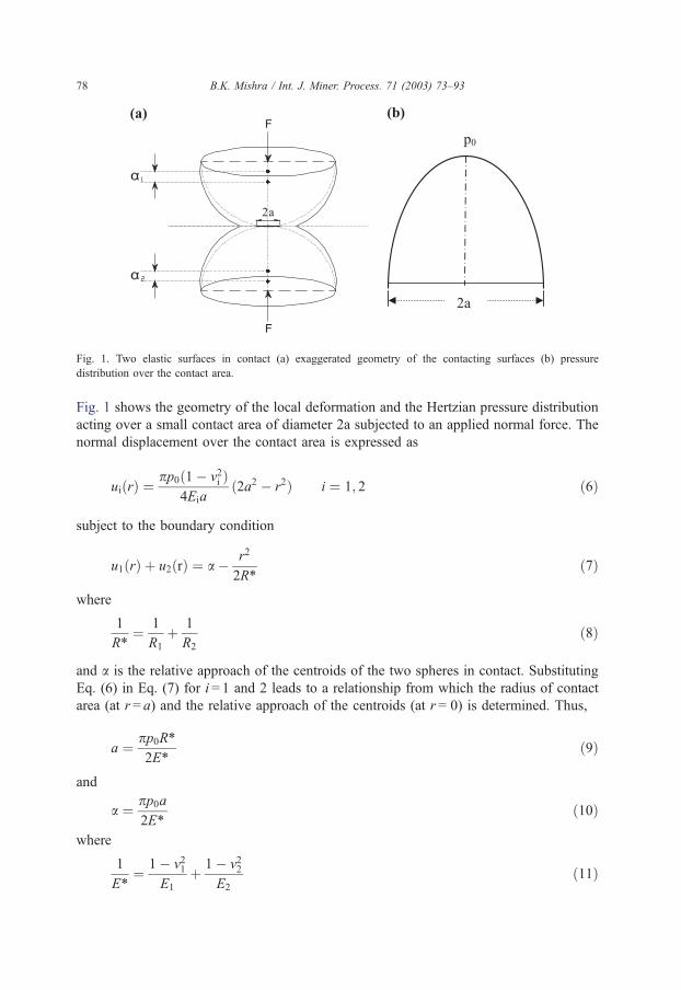
Fig. 1. Two elastic surfaces in contact (a) exaggerated geometry of the contacting surfaces (b) pressure

distribution over the contact area.


Fig. 1 shows the geometry of the local deformation and the Hertzian pressure distribution

acting over a small contact area of diameter 2a subjected to an applied normal force. The

normal displacement over the contact area is expressed as

uiðrÞ ¼pp0ð1� v2i Þ

4Eiað2a2 � r2Þ i ¼ 1; 2 ð6Þ

subject to the boundary condition

u1ðrÞ þ u2ðrÞ ¼ a � r2

2R*ð7Þ

where

1

R*¼ 1

R1

þ 1

R2

ð8Þ

and a is the relative approach of the centroids of the two spheres in contact. Substituting

Eq. (6) in Eq. (7) for i = 1 and 2 leads to a relationship from which the radius of contact

area (at r = a) and the relative approach of the centroids (at r = 0) is determined. Thus,

a ¼ pp0R*2E*

ð9Þ

and

a ¼ pp0a2E*

ð10Þ

where

1

E*¼ 1� v21

E1

þ 1� v22E2

ð11Þ


The contact normal force Fn is obtained by defining

Fn ¼Z a

0

pðrÞ2prdr ¼ 2

3p0pa

2 ð12Þ

Using (Eqs. (9), (10), and (12) the force–displacement relationship is obtained as

Fn ¼4

3E*R*1=2a3=2 ð13Þ

Recognizing that a=(R*a)1/2, the normal stiffness can be defined as

kn ¼dF

da¼ 2E*a ð14Þ

Unlike the linear contact model, according to the Hertzian contact law the normal stiffness

kn varies with the amount of overlap. Here again one can assume a very small amount of

overlap to evaluate the stiffness from the Hertzian model and use the value as a constant in

DEM models. Misra and Cheung (1999) limited the contact overlap to 0.5% of the ball

diameter and calculated the stiffness as 0.094ER which they kept constant during the

simulation. For spheroidal surfaces, Hertz theory is used to obtain the force deformation

relation needed to calculate the duration of impact and the maximum indentation. This

approach has been extended to the cases where constrained plastic deformation occurs.

Here, the force-deformation equation is augmented with a damping term to reflect

dissipation in the contact area.

2.2.3. The elastic perfectly plastic contact model

The major difficulty in implementing an approach based on a contact force model is

identifying parameters such as C for the viscous damping term in the force–displacement

relationship as stated in Eq. (2). One possible solution is to relate these unknown

parameters to the coefficient of restitution as done in Eq. (3). However, coefficient

restitution is not a constant; it is known to vary with relative impact velocity of colliding

bodies. At higher impact velocities, the coefficient of restitution is lower, meaning that

more energy is dissipated when the colliding bodies are moving faster. Faced with these

problems, Mishra and Thornton (2002) have eliminated the viscous dissipation term in the

force–displacement relationship with plastic dissipation, which is easy to determine from

the materials’ stress–strain curve.

An understanding of how yield occurs in contacts is needed to develop the appropriate

expression for the force indentation relation and to predict any damage due to plastic

deformation. If the relative impact velocity V between two colliding particles is just large

enough to initiate yield then using Eq. (13), we may write

1

2m*V 2

y ¼Z ay

0

Fnda ¼8E*a5y

15R*2ð15Þ


where Vy, which is defined as the yield velocity, is the relative impact velocity below

which the interaction behavior is assumed to be elastic, ay is the contact radius when yield

occurs, and m* is the effective mass given by

1

m*¼ 1

m1

þ 1

m2

ð16Þ

We now define a ‘limiting contact pressure’ py, which according to Eqs. (5) and (9) is

py ¼2E*ay

pR*ð17Þ

Combining Eqs. (15) and (17), we obtain

Vy ¼ 3:194p5yR*

3

E*4m*

!1=2

ð18Þ

In the case of a spherical ball of density q impacting with a plane surface, R* =R, and

m*=m, Eq. (14) reduces to

Vy ¼ 1:56p5y

E*4q

!1=2

ð19Þ

which relates the yield velocity of impact based on material properties.

In order to model the ‘post-yield’ behaviour, we adopt the approach taken by Thornton

and Ning (1998) who originally used the elastic perfectly plastic model to study the stick/

bounce behaviour of adhesive spheres. They argued that the normal force at yielding is

Fn ¼ Fe � 2pZ ap

o

½pðrÞ � py�rdr ð20Þ

where Fe is the equivalent elastic force required to produce the same total contact area

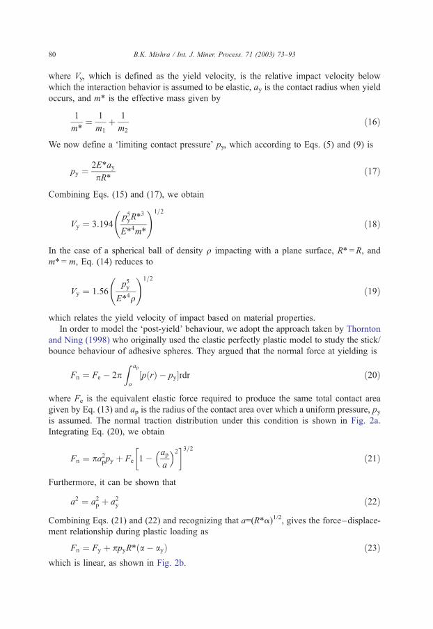
given by Eq. (13) and ap is the radius of the contact area over which a uniform pressure, pyis assumed. The normal traction distribution under this condition is shown in Fig. 2a.

Integrating Eq. (20), we obtain

Fn ¼ pa2ppy þ Fe 1� ap

a

� �2� �3=2ð21Þ

Furthermore, it can be shown that

a2 ¼ a2p þ a2y ð22Þ

Combining Eqs. (21) and (22) and recognizing that a=(R*a)1/2, gives the force–displace-

ment relationship during plastic loading as

Fn ¼ Fy þ ppyR*ða � ayÞ ð23Þwhich is linear, as shown in Fig. 2b.

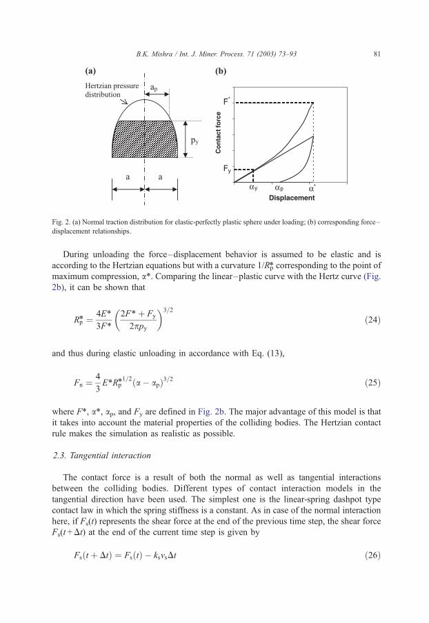
Fig. 2. (a) Normal traction distribution for elastic-perfectly plastic sphere under loading; (b) corresponding force–

displacement relationships.


During unloading the force–displacement behavior is assumed to be elastic and is

according to the Hertzian equations but with a curvature 1/Rp* corresponding to the point of

maximum compression, a*. Comparing the linear–plastic curve with the Hertz curve (Fig.

2b), it can be shown that

Rp* ¼ 4E*

3F*

2F*þ Fy

2ppy

�3=2

ð24Þ

and thus during elastic unloading in accordance with Eq. (13),

Fn ¼4

3E*Rp*

1=2ða � apÞ3=2 ð25Þ

where F*, a*, ap, and Fy are defined in Fig. 2b. The major advantage of this model is that

it takes into account the material properties of the colliding bodies. The Hertzian contact

rule makes the simulation as realistic as possible.

2.3. Tangential interaction

The contact force is a result of both the normal as well as tangential interactions

between the colliding bodies. Different types of contact interaction models in the

tangential direction have been used. The simplest one is the linear-spring dashpot type

contact law in which the spring stiffness is a constant. As in case of the normal interaction

here, if Fs(t) represents the shear force at the end of the previous time step, the shear force

Fs(t +Dt) at the end of the current time step is given by

Fsðt þ DtÞ ¼ FsðtÞ � ksvsDt ð26Þ


where ks is the tangential stiffness which assumes a constant value and vn is the tangential

component of the relative velocity of the particles. The value of the stiffness ks according

to Hertz–Mindlin contact theory may be taken to be 0.67 to 1. In the presence of friction,

slip occurs when the magnitude of the computed shear force exceeds the maximum

frictional resistance, and in that case the shear force assumes the limiting value lFn where

l is the friction coefficient. This type of contact law was incorporated in the earlier

Cundall and Strak’s (1979) model and it is still widely used.

The linear contact law can be improved by considering the model proposed by Mindlin

and Deresiewicz (1953). This model is for the elastic frictional contact between two

identical spheres in the tangential direction, subjected to varying normal, and tangential

forces. Thornton and Randall (1988) analyzed the loading case considered by Mindlin and

Deresiewicz and provided an incremental force–displacement relationship for the tangen-

tial direction. Walton and Braun (1986) proposed a simplified model based on the theory

of Mindlin and Deresiewicz. Details of these types of tangential interactions are reviewed

by Thornton (1999).

2.4. Numerical integration scheme

After deciding on a contact type, one can follow the dynamic equilibrium equation for a

particle in contact with several other particles. These equations can be written for each

coordinate axis, and both the translational and rotational equilibrium can be considered.

We discuss the numerical integration scheme by considering the following translational

equation of motion,

mxi þ Cxi þ Kx ¼ Fi ð27Þ

where Fi is the external force acting in the direction i and the parameters K and C are the

spring and dashpot constants. The form of the equation in Eq. (27) is linear, representing

the simple spring-dashpot contact model. Explicit numerical schemes are typically used in

the discrete element method to solve Eq. (27). A variety of explicit time integration

schemes are available. We have been quite successful with the leap frog type integration

scheme where the velocity of a particle is estimated at time step, say, n + 1/2, by knowing

the acceleration at the nth time step.

Here, the position and velocities are updated as follows:

ðxiÞNþ1 ¼ ðxiÞN þ ðxiÞNþ1=2 � Dt ð28Þ

ðxiÞNþ1=2 ¼ ðxiÞN�1=2 þ ðxiÞN � Dt ð29Þ

This means that each integration cycle involves three steps: calculation of (i) (xi)N�Dt

based on (xi)N, (ii) (xi)N + 1/2 and (iii) (xi)N + 1. The instantaneous velocity at the nth time

step is then calculated as

ðxiÞN ¼ðxiÞNþ1=2 þ ðxiÞN�1=2

2ð30Þ


The above explicit integration scheme is second-order accurate, and it is also regarded

as the best overall for accuracy, stability, and efficiency. Cundall and Strack (1979)

proposed a central difference scheme when the force balance equations on a particle

include global damping in addition to contact damping. The equation at that stage is mixed

with both the velocity and acceleration, and therefore the proposed modification to the

integration procedure is justified.

The time step for numerical integration should be set smaller than a certain critical

value to make the calculation stable. Based on the characteristic natural frequency of a

spring-mass oscillation system, the oscillation period can be calculated as

Dt ¼ 2pffiffiffiffiffiffiffiffiffiffim=K

pð31Þ

where m is the mass and K is the stiffness of the spring-mass system. In real systems, the

time step is calculated using the smallest mass and highest stiffness. A reduced time step is

typically considered to account for multi-particle collision situation, by dividing the

critical time step with a suitable number between 5 and 20.

3. Model parameters

The contact models that are used in DEM include parameters such as contact stiffness,

coefficient of restitution, and friction. One would like to develop models based on material

properties, but unfortunately, that is not the case for several reasons. For numerical

convenience and lack of reliable experimental data, often, compromise is made with

respect to choosing the correct parameters as will be shown in the following discussion.

Nevertheless, we discuss how best the parameters can be selected giving due importance

to the desired accuracy of the results and computational requirements.

3.1. Coefficient of restitution

In the light of elementary theory of impact, two limiting cases of impact can be

considered: perfectly elastic and perfectly inelastic. The former case implies that the

kinetic energy of the system is conserved. The latter case assumes that the two bodies

coalesce, to move as a single mass, after impact. The velocity of the combined mass

can then be predicted using only the conservation of momentum. However, most

impacts are neither fully elastic nor fully inelastic. This partial loss of the initial kinetic

energy is expressed in terms coefficient of restitution e. In many DEM simulations, the

coefficient of restitution is used as a constant parameter and accordingly, the energy

dissipation due to viscous damping has been made proportional to the coefficient of

restitution. But it is well known that the coefficient of restitution is not an intrinsic

material property; it depends on the materials of the bodies, their surface geometry and

the impact velocity (Johnson, 1985). An attempt is made here to deduce an expression

that would allow for the variation in the coefficient of restitution as a function of impact

velocity.


For a spherical ball impacting at a velocity Vi>Vy, the coefficient of restitution can be

directly calculated by considering the area under the force–displacement curve during

loading and unloading. Using Eq. (25), it can be shown that

1

2m*V 2

r ¼Z a*

ap

4

3E*R*1=2p ða � apÞ3=2da ð32Þ

where Vr is the rebound velocity, which with further manipulation, can be expressed as

V 2r ¼ 4

5

F*

m*ða*� apÞ ¼

6F*2

10E*m*a*ð33Þ

Thus, the coefficient of restitution can be obtained from

e2 ¼ 3F*2

5E*a*m*V 2i

ð34Þ

If the impact velocity is Vi =Vy, then no plastic deformation occurs, and ignoring energy

losses due to elastic wave motion in the colliding bodies, the coefficient of restitution

e = 1.0.

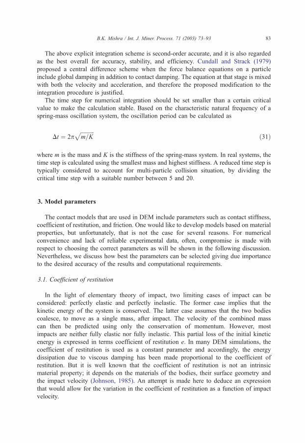
Numerical simulations of ball–ball collisions have been performed using the elastic

perfectly plastic contact model. In this simulation, a pair of steel balls of 4-cm and 5.4-cm

diameter was used where the smaller ball is allowed to normally impact the larger ball that

is at rest. Fig. 3 shows the effect of relative impact on the normal contact–force

displacement response. It is observed that for impact velocities greater than the yield

velocity, the unloading stiffness increases with increase in impact velocity. Consequently,

Fig. 3. Ball–ball impact test: effect of impact velocity on the normal contact force–displacement response.


the ratio of energy dissipated during loading to that during unloading depends on the

magnitude of the impact velocity and therefore the coefficient of restitution is velocity

dependent.

The coefficient of restitution can be experimentally determined for a much idealized

impact situation. However, in actual practice, it is easy to visualize that when a ball

impacts another ball inside the mill, the collision results in the movement of several other

balls, resulting in a multi-body impact situation. Under this situation, the coefficient of

restitution is difficult to estimate. However, it can be calculated on theoretical grounds, as

discussed earlier. The important issue here is that the coefficient of friction cannot be

treated as a constant.

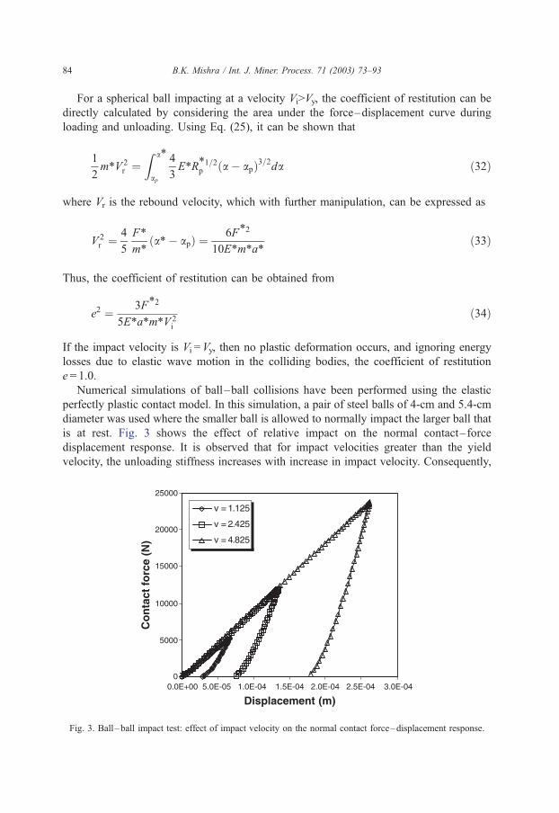
We show the simulation results for a 55-cm diameter mill to illustrate the idea of a variable

coefficient of restitution. Numerically, a ball mill of the exact configuration as that of an

experimental one (see Moys, 1993) was created to hold 2310 balls weighing 104.6 kg which

matched closely with the experimental load of 105 kg. Several simulations were carried out

in the fractional critical speed range of 0.6–1.1 at a constant mill filling. Fig. 4 shows the

distribution of impacts where the coefficient of restitution was calculated using Eq. (34),

where only the velocity before impact is considered, instead of the relative velocities before

and after impact. This distribution clearly shows that all impacts result in a coefficient of

distribution above 0.5. Furthermore, at 90% critical speed, it was observed that 79% of the

collisions resulted in coefficients of restitution in the range 0.9–1, increasing to 82% as the

mill speed was reduced to 60% of critical speed. This is an important observation in the light

of ball mill simulation where the coefficient of restitution is a key parameter that determines

the impact energy spectra and is often taken to be a constant b0.9, independent of the

impact velocity.

Fig. 4. Distribution of the coefficient of restitution; e is calculated according to Eq. (34).

3.2. Contact stiffness and damping

Contact stiffness is a key parameter that determines the overall dynamic behavior of the

particles. As mentioned earlier, the value of stiffness k is chosen in such a way that the

fraction of overlap in the most severe collision expected is a small fraction of the diameter

of the colliding element. This has been the practice where linear contact models are used.

However, in order to determine a more accurate estimate of the contact stiffness, Mishra

and Murty (2001) suggest an approximate method taking into account the actual material

response to collision. In their approach, the actual force–displacement relationship is

analyzed. These data can be obtained by using the ultrafast load cell (UFLC) that is used

extensively for generating single-particle breakage data. The force–displacement data is

fitted to a nonlinear differential equation that includes all the parameters of the contact

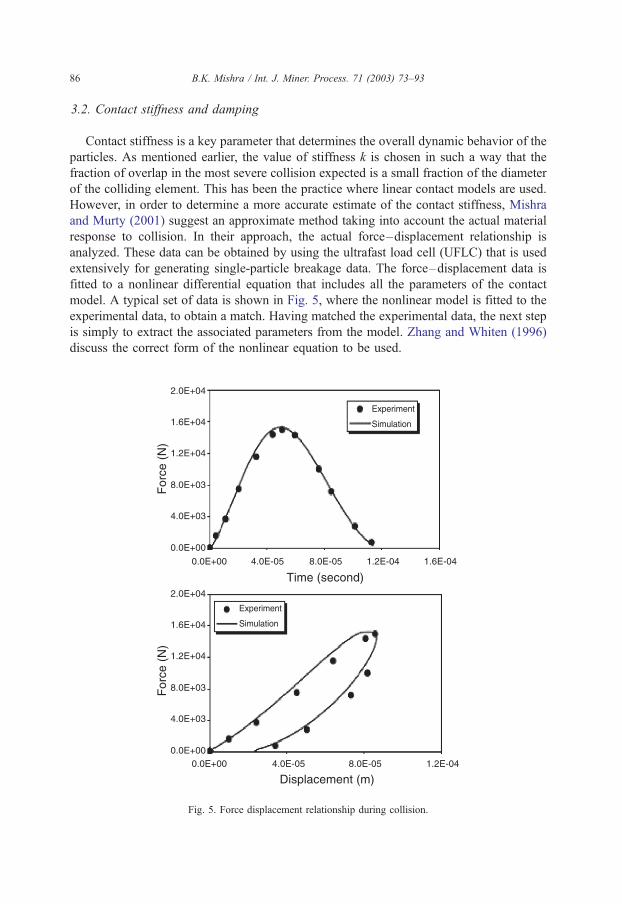
model. A typical set of data is shown in Fig. 5, where the nonlinear model is fitted to the

experimental data, to obtain a match. Having matched the experimental data, the next step

is simply to extract the associated parameters from the model. Zhang and Whiten (1996)

discuss the correct form of the nonlinear equation to be used.


Fig. 5. Force displacement relationship during collision.


Mishra and Murty (2001) went further and analyzed the numerical values of the

parameters. It was realized that these parameter (damping and contact) values were very

large that limit the critical time step, which when used as parameters in the DEM model

make the simulation too slow. For example, the stiffness for the set of data shown in Fig. 5

turns out to be of the order of 1010, which leads to a time step of the order of 10� 6 s. This

disadvantage can be overcome by using the equivalent linearization technique to transform

the nonlinear contact model to an analogous linear model. Not only did the linearized

parameters allow a larger time step, but also the use of a linear spring-dashpot model

significantly reduced the overall computational effort.

A linearized approximation to the force–displacement behavior was also implemented

by Walton and Braun (1986), albeit in a different manner. They proposed a partially

latching-spring model in which the unloading (linear) spring was stiffer than the loading

(linear) spring. If the unloading stiffness is a constant, this leads to a constant coefficient of

restitution equal to the square-root of the ratio of the loading/unloading stiffness. A

variable coefficient of restitution, which decreases with increasing impact velocity, was

obtained by allowing the unloading stiffness to increase with the maximum contact force

from which unloading commenced. In this way, a linearized approximation to the force–

displacement behavior shown can be obtained.

The form of the damping term in the force balance equation requires reexamination.

Typically, in DEM models, damping force is taken proportional to the relative velocity of

the colliding bodies. Zhang and Whiten (1996) noted that for the form of the DEM

equations generally used, the contact force could become very large at the first instance of

impact. This is not correct, as experiments show that the contact force must be zero when

t = 0 (see Fig. 3). This basically requires a correction term in the overall force balance

equation. Tsuji et al. (1992) arrived at the correction term heuristically to include a factor

in terms of the amount of overlap x as x1/4. This factor is included in the damping term that

now takes into account both the overlap and rate of overlap (see Eq. (2)). This way, when

t = 0, the contact force becomes zero.

3.3. Coefficient of friction

The coefficient of friction is difficult to measure, and it may vary during grinding.

While Cleary (1998) seemed to suggest that power draw is relatively insensitive to the

choice of value for coefficient of friction, Mishra and Rajamani (1992), Mishra and

Thornton (2001), and Van Nierop et al. (2001) showed that power draw of ball mills

indeed depends on the coefficient of friction, and it is particularly sensitive at higher mill

speeds. In one of the most carefully conducted tests using a laboratory size ball mill, Van

Nierop et al. (2001) observed that at mill speeds above the critical speed, the experimental

and DEM power results did not match. They argued that the coefficient of friction was not

sufficient for centrifuging to take place. In other words, balls lose traction and fall back to

the charge. They showed that by increasing the value of the coefficient of friction from

0.142 to 0.5, a better match of power draw between experimental and simulation data was

obtained at 160% critical speed.

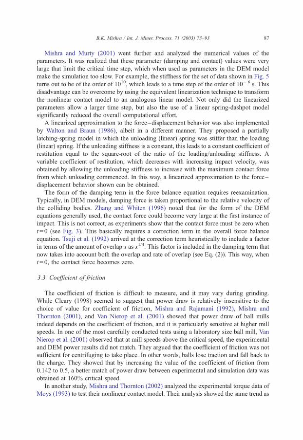
In another study, Mishra and Thornton (2002) analyzed the experimental torque data of

Moys (1993) to test their nonlinear contact model. Their analysis showed the same trend as

Fig. 6. Variation in torque with coefficient of friction.


observed by Van Nierop et al. (2001), i.e., a mismatch between the experimental and

simulated results. It was observed that up to 90% of the critical speed, the predicted torque

is within 7–8% of the experimental value. However, the predicted results diverged

significantly at 101.7% of critical speed. A series of DEM simulations was carried out

at 101.7% critical speed by varying the coefficient of friction. Results of these simulations

are shown in Fig. 6, where it is observed that by increasing the value of the coefficient of

friction to 0.4, a better agreement with the experimental result could be obtained. The

reason for the drop in the torque was a shift in the mode of the motion of the charge (for a

detailed description see Mishra and Thornton, 2001). In short, it is quite important to use

the most appropriate value of the coefficient of friction. Considering the dynamics of the

tumbling mill problem, it is in fact quite accurate to use a variable coefficient of friction

commensurate with the dynamics of the situation.

4. Computer implementation

Computer implementation of DEM is quite straightforward for regular elements. On the

other hand, dynamic problems involving irregular three-dimensional particles may become

quite difficult. Because of the sheer numbers of bodies (balls and rocks) and contacts

which must be tracked every time step (10 � 5 s), and with the number of time steps needed

for each simulation, it is vital to use algorithms and data structure that are efficient. In

order to minimize the computational time, one may use the Delaunay triangulation

method, which is commonly used for mesh generation in finite element analysis. In order

to determine the existence of a contact between a pair of bodies, it is only a matter of

checking the edge of the triangle that connects the pair of elements.

Most DEM code uses the cell technique to reduce the search space. In this

technique, the elements are sorted into a grid-cell-based data structure, as discussed


earlier. In general, a given disk occupies at most four cells, or a given ball occupies

eight cells in three dimensions. When the size of the cell is chosen to be greater than

the largest disk diameter, this ensures that a disk is located in a maximum of four cells.

This reduces the overall searching effort. However, there are situations where one

encounters a large gradation in the grinding media as in the case of semi-autogenous

(SAG) mills. These mills are typically 10–12 m in diameter, and the size of the media

may vary from 15 to 2 cm. Since the cell size is limited by the size of the largest

grinding media, the search effort increases drastically in proportion to the gradation in

the charge.

The integration of DEM equations requires a specific model for the contact force. These

models, as discussed earlier, range from the simplest linear model to a more realistic

Hertzian-type model. For many applications, a Hertzian-type model may not be an

accurate description of the contact behavior. For example, the geometry of the colliding

bodies may not be as simple as was assumed in developing the above relationship. It

should be realized that from a practical standpoint, it might not be important to reveal all

the minute details of the interactions at the contact as long as the overall behavior of the

system as a whole is satisfactory. This is precisely why the contact model used in DEM for

most comminution applications is that of a stiff linear spring of spring constant k. The

value of stiffness k is chosen in such a way that the fraction of overlap in the most severe

collision expected is a small fraction of the diameter of the colliding element which may

be a disk or ball.

The major disadvantage of DEM is the requirement of an enormous amount of

computational time. This is due to the explicit nature of the algorithm that requires a

very small time step of simulation to assure numerical stability and accuracy. As in

Molecular Dynamics, the computer code tracks a large number of individual entities, from

a few thousands in the 2D simplified model to hundreds of thousands in the actual 3D

model. In addition, there is no steady state and the evolution of the system is calculated for

small increments of time of the order of 10–4 s. Therefore, similar sets of calculations are

repeated billions of times for any realistic simulation. As a result realistic DEM simulation

in the comminution area has not progressed significantly past the two-dimensional stage.

However, DEM naturally renders itself for parallelization. One can develop a flexible

parallel computer code that is capable of generating external shell, internal surfaces and

multibody assemblies for carrying out simulations to track particle trajectory and even

fragmentation. Current applications of the discrete element method on parallel computers

have been gaining importance (Ghaboussi et al., 1993; Ferrez et al., 1996; Sawley and

Cleary, 1999; Hentry, 2000), and as the problem size increases, parallelization will become

even more common.

Once implemented, DEM can be applied to any comminution problem. DEM can

simulate a whole range of comminution devices such as a SAG mill, ball mill, planetary

mill, etc. It has now become possible to carry out three-dimensional DEM simulations

comprising 10,000 balls in personal computers. This has increased its popularity by leaps

and bounds. Today, there are at least a dozen companies worldwide using DEM on a

routine basis for systematic plant analysis. In the second part of the paper, we show some

of the interesting application areas relating to tumbling mills where DEM has made major

headway.


5. Analysis of a single ball impact

A vast amount of data can be obtained from a simple impact test of a ball. It is the most

fundamental and frequent event that occurs inside a ball mill, and therefore corresponding

experiments must be carried out as accurately as possible. In order to model impact events

in a simulation, several types of contact models can be considered. A linear contact model

using a pair of spring and dashpot to represent the contact interaction between colliding

balls would describe the normal contact force as

Fn ¼ knDxþ Cnvn ð35Þ

where kn is the contact stiffness, Cn is a dashpot parameter that can be related to the

coefficient of restitution, Dx is the amount of relative approach (overlap), and vn is the

relative velocity in the normal direction. In order to make the contact response more

realistic, a Hertzian nonlinear model for the contact can be assumed such that

Fn ¼4

3E*R*1=2Dx3=2 þ Cnvn ð36Þ

where E* and R* are defined according to Eqs. (8) and (11). The damping term in either

model could be a function of displacement and velocity. These models were simulta-

neously used along with the elastic perfectly plastic contact model to simulate the impact

behavior of a ball.

The results of the single-ball impact test at an impact velocity of 2.425 m/s is presented

in Fig. 7 which shows separately the variations in the contact force with time (left) and

with displacement (right). The first observation is that the contact force in the linear as well

as nonlinear viscoelastic case does not look realistic, insofar as the contact force becomes

negative towards the end of the collision period. Furthermore, in the linear case, the

contact force is finite at time t = 0. These issues are adequately discussed in the literature

(see Zhang and Whiten, 1996). In order to make the initial contact force zero, several

researchers use the damping term not only as a function of the impact velocity but also of

the displacement. Furthermore, since a negative contact force is unrealistic, the contact

Fig. 7. Force versus time and displacement using three different contact models.


must break at a time when the contact force is zero. Despite these numerical adjustments,

the plastic deformation at the contact is not fully explained. Instead, using the elastic

perfectly plastic contact model, the dashpot is entirely eliminated. The result of the

simulation using the elastic perfectly plastic contact model is also shown in Fig. 7. It is

observed from the contact response corresponding to the elastic perfectly plastic contact

model that the contact force is zero at time t = 0, and it again becomes zero when the

contact is broken. The contact breaks at a time when the contact force becomes zero (tf = 0),

not when the contact overlap becomes zero (tDx = 0).

6. Conclusions

Given the increasing need to simulate the behavior of grinding media in tumbling

mills accurately and precisely, this review paper describes a popular computational

model known as the discrete element method (DEM). It enables simulation of even

the largest mills involving spherical steel balls and irregular-shaped rocks. In par-

ticular, the paper explores how interparticle force laws and the associated contact para-

meters affect the accuracy of the computational results. An important part of showing

the effectiveness of the numerical scheme in solving the tumbling mill problem is to

demonstrate its inherent adaptability. Thus, certain other issues involving computa-

tion time, memory management, and various other implementation aspects are dis-

cussed.

In order to successfully simulate the tumbling mill, a realistic contact force model

must be included into the equations of motion to analyze the charge dynamics. A variety

of contact models is available ranging from simple linear-spring dashpot type to the most

sophisticated Hertz–Mindlin contact theory. Unfortunately, there are two major difficul-

ties with most of these models. First, one has to use the proper form of the contact force

equation, and second, the equation’s parameters must be identified. Although Hertz

theory helps in this regard, many contacts that occur in practice are of the non-Hertzian

type. Therefore, beyond the yield point, the force–displacement relationship can be

determined by considering elastic plastic contact. For this analysis, the rigid perfectly

plastic material model is commonly used. This type of model automatically produces

coefficient of restitutions that are function of impact velocity and only requires material

properties as input parameters.

References

Barker, G.C., 1994. Computer simulations of granular materials. In: Mehta, A. (Ed.), Granular Matter: An

Interdisciplinary Approach. Springer-Verlag, New York, pp. 35–83.

Campbell, C.S., 1990. Rapid granular flows. Annu. Rev. Fluid Mech. 22, 57–92.

Chang, C.S., Acheeampong, K.B., 1993. Accuracy and stability for static analysis using dynamic formulation in

discrete element method. In: Williams, J.R., Mustoe, G.G.W. (Eds.), Proceedings of the 2nd International

Conference on the Discrete Element Method, pp. 379–389. 1st IESL Publication Edition, MA, USA.

Cleary, P.W., 1998a. Predicting charge motion, power draw, segregation, wear and particle breakage in ball mills

using discrete element methods. Miner. Eng. 11 (11), 1061–1080.


Cleary, P.W., 1998b. The filling of dragline buckets. Math. Eng. Ind. 7, 1–24.

Cundall, P.A., 1988. Formulation of a three dimensional distinct element model. Part I: a scheme to detect and

represent contacts in a system composed of many polyhedral blocks. Int. J. Rock Mech. 25, 107–116.

Cundall, P.A., Strack, O.D.L., 1979. A discrete numerical model for granular assemblies. Geotechnique 29,

47–65.

Ferrez, J.-A., Muller, D., Liebling, T.M., 1996. Parallel implementation of a distinct element method for granular

media simulation on the Cray T3D. EPFL Supercomput. Rev. 8, 4–7.

Flavel, M.D., Rimmer, H.W., 1981. Particle breakage study in an impact breakage environment. Reprint of paper

presented at SME-AIME Annual Meeting, Chicago, USA. SME Publications, Littleton, Ohio.

Ghaboussi, J., Barbosa, R., 1990. Three dimensional discrete element method for granular materials. Int. J.

Numer. Anal. Methods Geomech. 14, 451–472.

Ghaboussi, J., Basole, M.M., Ranjithan, S., 1993. Three dimensional discrete element analysis on massively

parallel computers. In: Williams, J.R., Mustoe, G.G.W. (Eds.), Proceedings of the 2nd International Confer-

ence on the Discrete Element Method, pp. 95–104. 1st IESL Publication Edition, MA, USA.

Hentry, D.S., 2000. Performance of hybrid message-passing and shared-memory parallelism for discrete element

modeling. Proceedings of Super Computing 2000, Dallas, USA.

Hoyer, D.I., 1999. Discrete element method for fine grinding scale-up in Hicom mills. Powder Technol. 105 (1),

250–256.

Inoue, T., Okaya, K., 1996. Grinding mechanisms of centrifugal mills—a batch ball mill simulator. Int. J. Miner.

Process. 44 (45), 425–435.

Johnson, K.L., 1985. Contact Mechanics. Cambridge Univ. Press, Cambridge, UK.

Mindlin, R.D., Deresiewicz, H., 1953. Elastic spheres in contact under varying oblique forces. J. Appl. Mech. 20,

327–344.

Mishra, B.K., 1991. Study of media mechanics in tumbling mills. PhD Thesis. Department of Metallurgical

Engineering, University of Utah.

Mishra, B.K., Murty, C.V.R., 2001. On the determination of contact parameters for realistic DEM simulations of

ball mills. Powder Technol. 115 (3), 290–297.

Mishra, B.K., Rajamani, R.K., 1990. Numerical simulation of charge motion in ball mills. Proceedings of the 7th

European Conference on Comminution, Ljubljan, 555–570.

Mishra, B.K., Rajamani, R.K., 1992. The discrete element method for the simulation of ball mills. Appl. Math.

Model 16, 598–604.

Mishra, B.K., Thornton, C., 2001. Impact breakage of particulate agglomerates. Int. J. Miner. Process. 61,

225–231.

Mishra, B.K., Thornton, C., 2002. An improved contact model for ball mill simulation by the discrete element

method. Adv. Powder Technol. 13 (1), 25–41.

Misra, A., Cheung, J., 1999. Particle motion and energy distribution in tumbling mills. Powder Technol. 105,

222–227.

Moys, M.H., 1993. A model for mill power as affected by mill speed, load volume and liner design. J.S. Afr. Inst.

Min. Metall. 6–93, 135–141.

Mujinza, A., Bicnic, N., Owen, D.R.J., 1993. BSD contact detection algorithm for discrete elements in 2D. In:

Williams, J.R., Mustoe, G.G.W. (Eds.), Proceedings of the 2nd International Conference on the Discrete

Element Method, pp. 39–52. 1st IESL Publication Edition MA, USA.

Rajamani, R.K., Mishra, B.K., 1996. Dynamics of ball and rock charge in SAG Mills. Proceedings of the SAG

Conference, Vancouver, Canada, October 7–9, 700–712.

Sawley, M.L., Cleary, P.W., 1999. A parallel discrete element method for industrial granular flow simulations.

EPFL Supercomput. Rev. 11.

Thornton, C., 1999. Interparticle relationships between forces and displacements. In: Oda, M., Iwashita, K.

(Eds.), Mechanics of Granular Materials. Balkema, Netherlands, pp. 207–217.

Thornton, C., Ning, Z., 1998. A theoretical model for the stick/bounce behavior of adhesive, elastic-plastic

spheres. Powder Technol. 99, 154–162.

Thornton, C., Randall, W., 1998. Applications of theoretical contact mechanics to solid particle system

simulation. In: Satake, M., Jenkins, J.T. (Eds.), Micromechanics of granular materials. Elsevier, Amsterdam,

pp. 133–142.


Ting, J.M., 1992. A robust algorithm for ellipse based discrete element modeling of granular materials. Comput.

Geotech, 129–146.

Ting, J.M., Corkum, B.T., 1992. A computational laboratory for discrete element geomechanics. J. comput. Civ.

Eng. ASCE 6, 129–146.

Tsuji, Y., Tanaka, T., Ishida, T., 1992. Lagrangian simulation of plug flow of cohesionless particles in a horizontal

pipe. Powder Technol. 71, 239–250.

Van Nierop, M.A., Glover, G., Hinde, A.L., Moys, M.H., 2001. A discrete element method investigation of the

charge motion and power draw of an experimental two-dimensional mill. Int. J. Miner. Process. 59, 131–148.

Walton, O.R., 1994. Numerical simulation of inelastic frictional particle–particle interaction. In: Roco, M.C.

(Ed.), Particulate Two-Phase Flow, pp. 884–911. Chap. 25.

Walton, O.R., Braun, R.L., 1986. Viscosity, granular-temperature, and stress calculations for shearing assemblies

of inelastic, frictional disks. J. Rheol. 30, 949–980.

Williams, J.R., O’Connor, R., 1995. A linear complexity intersection algorithm for discrete element simulation of

arbitrary geometries. Eng. Comput. 12, 185–201.

Williams, J.R., O’Connor, R., Rege, N., 1996. Discrete element analysis and granular vortex formation. Electron.

J. Geotech. Eng. (premier issue).

Zhang, D., Whiten, W.J., 1996. The calculation of contact forces between particles using spring and damping

models. Powder Technol. 88, 59–64.

Zhang, R., Mustoe, G.G.W., Nelson, K.R., 1993. Simulation of hydraulic phenomena using the discrete element

method. In: Williams, J.R., Mustoe, G.G.W. (Eds.), Proceedings of the 2nd International Conference on the

Discrete Element Method, pp. 189–200. 1st IESL Publication Edition, MA, USA.

Documents

A review of computer simulation of tumbling mills by the discrete element method: Part I—contact mechanics