Embed Size (px)
Citation preview

A REPLICATION STRATEGY
FOR
DISTRIBUTED REAL-TIME OBJECT ORIENTED DATABASES
BY
PRAVEEN PEDDI
A THESIS SUBMITTED IN PARTIAL FULFILLMENT OF THE
REQUIREMENTS FOR THE DEGREE OF
MASTER OF SCIENCE
IN
COMPUTER SCIENCE
UNIVERSITY OF RHODE ISLAND
2001
ii
MASTER OF SCIENCE THESIS
OF
PRAVEEN PEDDI
APPROVED:
Thesis Committee
Major Professor ____________________________
____________________________
____________________________
____________________________DEAN OF THE GRADUATE SCHOOL
UNIVERSITY OF RHODE ISLAND
2001

i
Abstract
In many real-time applications such as command and control, industrial automation,
aerospace and defense systems, telecommunications data is naturally distributed
among several locations. Often this data must be obtained and updated in a timely
fashion. But sometimes data that is required at a particular location is not available,
when it is needed and getting it from remote site may take too long before which the
data may become invalid, violating the timing constraints of the requesting
transaction.
One of the solutions, for the above-mentioned problem, is replication of data in real-
time databases. This makes the data available locally on the requested site.
Unfortunately, very little research is involved in replicating the data in real-time
databases, especially in real-time object-oriented databases.
We have developed an algorithm called Just-In-Time Real Time Replication (JITRTR)
algorithm that generates replication transactions that copy required data where and
when it is needed. The algorithm takes the requests and updates from the
specifications and translates them into local transactions. It also analyzes the
parameters of the requests and updates and creates replication transactions so that all
the requests always read valid data at any point of time. The JITRT replication
algorithm takes care that all requests always read valid data. The algorithm has two
versions. The first version deals with requests or updates made on the full object.
Second version deals with requests made on the methods of objects.

ii
Acknowledgement:
I would like to thank my academic advisor Dr Lisa Cingiser Dipippo for her guidance
and encouragement through out my masters program. I would like to thank Dr Victor
Fay Wolfe for his valuable advices many times when I was stuck in the middle of the
research.
I wish to thank all the members of the real-time research group in University of Rhode
Island for their time and input. I am grateful to Dr Gray for his consent to serve on my
thesis committee. I am indebted to all the members of faculty in computer science
department who have helped in some way or other towards my master’s degree,
especially Dr Joan Peckham.
I also thank Ben Watson and Sam Naiser of Tripacific Inc. for helping in giving the
licensed copy of Rapid RMA, the tool I used to determine schedulability of the
system.
My special thanks to my brother Pramodh Peddi, who co-operated and helped me
when I was suffering from back pain during my graduate studies. Without his help, it
would have been very difficult for me to finish my studies smoothly.
I also like to thank Lorraine and Marge for making computer science department a
wonderful place to study.

iii
Preface:
The thesis is organized as follows. Chapter 1 gives the introduction of the algorithms
we have developed. Chapter 2 gives the background material that is closely related to
the thesis. Chapter 3 gives the detailed explanation of the JITRT replication algorithms
for full object and affected sets. Chapter 4 states and proves three theorems that
demonstrate the correctness and goodness of the algorithm. Chapter 5 gives the
implementation methodology of the algorithms. Chapter 6 presents the results of a
series of test suites that we performed comparing our algorithm with other replication
strategies. Chapter 7 gives the conclusion of the thesis work. Chapter 8 lists the future
work that can be done based on the present thesis. Then the list of references is given.
The final part consists of two appendices. Appendix A details the implementation of
the algorithm based on full object requests. Appendix B details the implementation of
the algorithm based on method requests.
iv
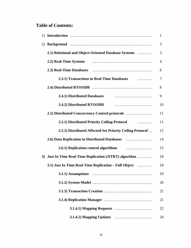
Table of Contents:
1) Introduction ………………………………………………………… 1
2) Background ………………………………………………………… 3
2.1) Relational and Object-Oriented Database Systems ………… 3
2.2) Real-Time Systems ………………………………………… 4
2.3) Real-Time Databases ………………………………………… 6
2.3.1) Transactions in Real-Time Databases ………… 7
2.4) Distributed RTOODB ………………………………………… 8
2.4.1) Distributed Databases ………………………… 9
2.4.2) Distributed RTOODB ………………………… 10
2.5) Distributed Concurrency-Control protocols ………………… 11
2.5.1) Distributed Priority Ceiling Protocol ………… 11
2.5.2) Distributed Affected-Set Priority Ceiling Protocol … 12
2.6) Data Replication in Distributed Databases ………………… 14
2.6.1) Replication control algorithms ………………… 15
3) Just In Time Real-Time Replication (JITRT) algorithm ………… 18
3.1) Just In Time Real-Time Replication – Full Object ………… 18
3.1.1) Assumptions ………………………………………… 19
3.1.2) System Model ………………………………………… 20
3.1.3) Transaction Creation ………………………………… 21
3.1.4) Replication Manager ………………………………… 21
3.1.4.1) Mapping Requests ………………………… 22
3.1.4.2) Mapping Updates ………………………… 24

v
3.1.5) Mapping of Transactions to DPCP model ………… 26
3.1.6) Execution Model ………………………………… 27
3.1.7) Examples ………………………………………… 27
3.2) Just In Time Real-Time Replication – Affected Set………… 30
3.2.1) Assumptions ………………………………………… 31
3.2.2) System Model ………………………………………… 31
3.2.3) Transaction Creation ………………………………… 32
3.2.4) Replication Manager ………………………………… 33
4) Analysis ………………………………………………………… 36
4.1) Theorems ………………………………………………… 36
5) Implementation Methodology ………………………………… 42
6) Testing ………………………………………………………… 44
6.1) Test Generation ………………………………………………… 44
6.2) Performance Measures ………………………………………… 45
6.3) JITRT-FO Testing ………………………………………… 46
6.3.1) Test Suites ………………………………………… 46
6.3.1.1) Baseline testing ………………………… 46
6.3.1.2) Test Suite 1 ………………………………… 47
6.3.1.3) Test Suite 2 ………………………………… 47
6.3.1.4) Test Suite 3 ………………………………… 48
6.3.2) Results ………………………………………………… 49
6.3.2.1) Baseline testing ………………………… 49
6.3.2.2) Test Suite 1 ………………………………… 50

vi
6.3.2.3) Test Suite 2 ………………………………… 52
6.3.2.4) Test Suite 3 ………………………………… 54
6.4) JITRT-AS Testing ………………………………………… 55
6.4.1) Test Suites ………………………………………… 55
6.4.1.1) Baseline testing ………………………… 55
6.4.1.2) Test Suite 1 ………………………………… 56
6.4.2) Results ………………………………………………… 57
6.4.2.1) Baseline testing ………………………… 57
6.4.2.2) Test Suite 1 ………………………………… 58
6.5) Effect of number of remote requests and updates on JITRT-FO 60
7) Conclusion ………………………………………………………… 61
8) Future Work ………………………………………………………… 63
9) References ………………………………………………………… 65
10) Appendix A - Implementation details of JITRT-FO ………… 69
11) Appendix B - Implementation details of JITRT-AS ………… 76
12) Appendix C – Sample configuration file generated by JITRT … 83

vii
List of Tables
1) Table 6.1 - Parameter Ranges for Baseline Testing (JITRT-FO) …… 46
2) Table 6.2 Ranges of Period for Test Suite 1 …………………………… 47
3) Table 6.3 Ranges of number of objects for Test Suite 2 …………… 48
4) Table 6.4 Value of percentage of updates for Test Suite 3 …………… 48
5) Table 6.5 - Parameter Ranges for Baseline Testing (JITRT-AS) …… 56
6) Table 6.6 – Ranges of WAS for test suite 1 …………………… 56

viii
List of Figures
1) Figure 3.1 – JITRT algorithm methodology ………………… 19
2) Figure 3.2 – Invalid Interval – 1 ………………………… 24
3) Figure 4.1 – Invalid Interval – 2 ………………………… 37
4) Figure 4.2 - Deadline Assignment 1 ………………………… 39
5) Figure 4.3 - Deadline Assignment 2 ………………………… 39
6) Figure 4.4 - Deadline Assignment 3 ………………………… 40
7) Figure 5.1 - System Execution ………………………… 43
8) Figure 6.1 – Test Generation ………………………… 45
9) Figure 6.2 – Shedulability for Baseline Testing ………………… 49
10) Figure 6.3 – Task Schedulability for Baseline Testing ………… 50
11) Figure 6.4 – System Schedulability Results on Effect of Period… 51
12) Figure 6.5 – Task Schedulability Results on Effect of Period … 52
13) Figure 6.6 – System Schedulability Results on No of objects … 53
14) Figure 6.7 – Task Schedulability Results on Effect of No of objects 53
15) Figure 6.8 – System Sched Results on effect of update percentage 54
16) Figure 6.9 – Task Sched Results on Effect of update percentage… 55
17) Figure 6.10 – System Schedulability for Baseline Testing … 57
18) Figure 6.11 – Task Schedulability for Baseline Testing………… 58
19) Figure 6.12 System Schedulability Results on Effect of WAS … 59
20) Figure 6.13 Task Schedulability Results on Effect of WAS … 59
21) Figure 6.14 Test with all remote requests (JITRT-FO) ………… 60

1
Chapter 1
Introduction
As computers have become essential parts of our daily activities, real time computing
is emerging as an important discipline and an open research area in computer science
and engineering. Many real time systems are now being used in safety critical
applications in which human lives or expensive machinery may be at stake. Their
missions are often long lived making maintenance and reconfiguration difficult.
Examples of such applications include command and control, industrial automation,
aerospace and defense systems, telecommunications etc. The demands of the operating
environment of such systems often pose rigid requirement on their timely
performance. To satisfy these requirements, the system may need to trigger necessary
transactions (Real-Time) to react to the critical events.
Transactions in real time databases (RTDB) should not only consider logical
consistency but also consider timing constraints and temporal consistency of the data.
Temporally consistent data may be valid only for a short interval of time. Maintaining
temporal consistency in real time databases is very difficult due to its unpredictable
data access. Recently, developers of real-time systems have recognized the need for
research in database systems that satisfy timing constraint requirements in reading and
updating data. On the other hand, many of the above-mentioned applications are
globally distributed rather than centralized and an application at one site requires
communication with the same application at another site. This forces the need for a
distributed version of the real time database system. Applying the principles of real

2
time systems and the database systems complicates issues like communication
between a database on one site and a database on the other site, concurrency control,
maintaining temporal consistency, etc. The added communication costs makes the
timing property of the requests on the remote site more unpredictable. Therefore
accessing or updating data on the local site may take less time than that on the remote
site. One of the solutions, to make the data available on the local site and minimize the
response time, is replication of data from the remote site to the local site. But to
maintain the validity of data, the replication strategy should consider real time
parameters like period and deadline of the requesting transactions.
This thesis presents two replication algorithms called Just In Time Real-Time Full
Object (JITRT-FO) replication and Just In Time Real-Time Affected Set (JITRT-
AS) replication that generates replication transactions to copy the required data where
and when it is needed and guarantees that the copy is always valid. JITRT-FO deals
with the full object and JITRT-AS deals with affected sets. The paper also presents
three theorems that indicate the necessity of the deadline assignment of our algorithm,
and that all requests read valid data with the JITRT-FO and JITRT-AS algorithms.
The rest of this thesis is organized as follows. Chapter 2 gives the background material
related to the thesis. Chapter 3 gives the detailed explanation of the JITRT replication
algorithms for full object and affected sets. Chapter 4 states and proves three theorems
that demonstrate the correctness and goodness of the algorithm. Chapter 5 gives the
implementation methodology of the algorithms. Chapter 6 presents the results of a
series of test suites that we performed comparing our algorithm with other replication
strategies.

3
Chapter 2
Background
This section gives background information related to relational and object-oriented
databases, real-time systems, real-time databases, distributed databases and distributed
concurrency control protocols.
2.1) Relational and Object-Oriented Database Systems:
The relational database model was first introduced by Ted Codd of IBM research in
1970 and attracted immediate attention due to its simplicity. It represents the database
as a collection of relations [10]. This model has been very successful in developing the
database technology required for many traditional business database applications. But
it has certain limitations when more complex database applications must be designed
and implemented. Examples of such complex database applications include database
for engineering design & manufacturing (CAD/CAM & CIM), scientific experiments,
telecommunications, Geographical Information Systems (GIS), multimedia etc. These
applications have requirements and characteristics that differ from those of traditional
business applications, such as complex structures for objects, longer duration
transactions, user defined data types for storing image objects and large textual items.
Object oriented databases (OODB) were proposed to meet the requirements of the
above applications. OODBs have proven to be more flexible to handle these
requirements without being limited by data types and query languages available in
traditional database systems. A powerful advantage of OODB over relational
databases is the ability to specify the structure of complex objects and the methods that

4
can be applied to these objects. Another reason why OODB have become important is
that they are based on the concepts of object-oriented programming languages.
Increasing use of object-oriented programming languages in developing software
applications and ease of embedding OODB in object-oriented software applications
developed in object-oriented programming languages like C++, SMALLTALK, JAVA
etc. have also made OODB more attractive. Examples of prototypes of OODB include
ORION, Open OODB, IRIS etc. Examples of commercial databases include
GEMSTONE/OPAL, ONTOS, Objectivity etc. Object Data Management Group
(ODMG), which is a standard organization, has become the standard for most of the
OODB [10].
Due to the above advantages of OODB, in this thesis project, we plan to use object-
oriented version of database rather than relational version.
2.2) Real-Time Systems:
A real-time system is one in which the correctness of the computations not only
depends upon the logical correctness of the computation but also upon the time at
which the result is produced. If the timing constraints of the system are not met,
system failure is said to have occurred [28]. So, data in real-time databases has to be
logically and temporally consistent. The latter arises from the need to preserve the
temporal validity of data items that reflect the state of the environment that is being
controlled by the system [25]. There can be made a classification into hard and soft
real-time systems based on their properties.
5
Hard Vs Soft real-time system:
In hard real time system, no lateness (missing deadline) is accepted under any
circumstances. This will result in catastrophic failure and the cost of missing deadline
is infinitely high [26]. This type of system should guarantee the timing constraints a
priori. An example of a hard real time system is a digital fly-by-wire control system of
an aircraft. In this, lateness may result in catastrophic failure and the result may be a
hole in the ground. The lives of people depend on the correct working of the control
system of the aircraft.
In soft real time system, missing deadline is allowed but may result in increase of the
cost. It does not result in any catastrophic failure. One example of a soft real-time
system is a multimedia application in which there is a relatively high tolerance for
missing deadlines related to decompressing sound or video. Such failures might result
in temporary degradation of output quality, but the presentation itself remains largely
intact. However the users are often are often willing to tolerate a few glitches, as long
as the glitches occur rarely and for short lengths of time [24].
Static Vs Dynamic systems:
A static system is one in which all of the system specifications are known a priori and
do not change once the system starts.
A dynamic system is a system in which new specifications can be added or the old
specifications can be changed even after the system is started.

6
2.3) Real-Time Databases:
Traditional databases deal with persistent data. Transactions access data while
maintaining its consistency. Serializability is the usual correctness criterion associated
with these transactions. The goal of transactions and query processing approaches
adopted in databases is to achieve a good throughput and response time. Many real
world applications involve time-constrained access to data as well as access to data
that has temporal validity. For example, consider telephone-switching systems,
program stock trading, managing automated factories and command and control
systems. Such applications introduce the need for real-time database systems. The area
of real-time database systems has attracted the attention of researchers in both real-
time systems and database systems. The motivation of the database researchers has
been to bring to bear many of the benefits of database technology to solve the
problems in managing the data in real-time systems [13].
Real-Time databases, for the most part, deal with temporal data, data that becomes
outdated after a certain time or data that is valid for some certain period of time. Due
to temporal nature of data and response time requirements imposed by the
environment, transactions in real-time databases possess timing constraints like period
or deadline. The resulting important difference is that the goal of real-time databases is
to meet the timing constraints of the activities [3]. Transactions in real-time database
systems should be scheduled considering both data consistency and timing constraints
[2]. In addition to the timing constraints that arise from the need to continuously track
the environment, timing correctness requirements in real-time database systems also
arise because of the need to make data available to the controlling system for its

7
decision-making activities. The need to maintain consistency between the actual state
of the environment and the state reflected by the contents of the database leads to the
notion of temporal consistency.
Adding the object-oriented features to the traditional real-time databases will provide
all the benefits of the real-time databases as well as object-oriented databases, but also
will complicate many of the issues. Many of the real-time applications discussed
above deal with complex data. So, a real-time object-oriented database system
(RTOODB) solves many of the problems with complex data.
2.3.1) Transactions in Real-Time Databases:
The nature of transactions in real-time databases can be characterized along 3
dimensions [13]:
1) Manner in which data is used by transactions: A Real-Time database systems
employ all three types of transactions that are employed in the traditional database
systems.
• Write-only transactions obtain state of the environment and write into
the database.
• Update transactions derive new data and store in the database.
• Read-only transactions read data from the database and send them to
actuators.
2) The nature of timing-constraints: Some transaction timing constraints come
from temporal consistency requirements and some come from requirements
imposed on the system reaction time. Temporal consistency requirements take the

8
form of periodicity requirements. System reaction requirements typically take the
form of deadline constraints imposed on aperiodic transactions.
3) Significance of executing transactions by its deadline: Transactions can also be
distinguished based on the effect of missing transaction’s deadline. They are hard,
soft and firm transactions.
• Hard deadline transactions are those that may result in a catastrophe if the
deadline is missed. These are typically safety-critical activities, such as those
that respond to life or environment-threatening emergency situations.
• Soft deadline transactions have some value even after their deadline. Typically
the value drops to zero at a certain pints after the deadline.
• Firm deadline transactions are those whose value drops to zero exactly after
the deadline, i.e. they have no value after their deadline expires [13].
The processing of transactions in real-time database systems is more complicated than
that in traditional database systems. Since meeting timing-constraints is the goal, it is
important to understand how transactions are scheduled and how their scheduling
relates to time constraints. So, absolute validity requirements on the data induce
periodicity requirements.
2.4) Distributed RTOODB:
Many of the real-time applications like command and control, defense systems,
aerospace, telecommunications are distributed globally rather than centralized at one
place. So, a centralized real-time object-oriented database may not be sufficient for
9
such applications. This leads to the need for making the Real-Time object-oriented
database systems (RTOODB) distributed globally.
2.4.1) Distributed Databases:
A distributed database (DDB) is a collection of multiple logically interrelated
databases distributed over a computer network and a distributed database management
system (DDBMS) is a software system that manages a distributed database making the
distribution transparent to the user [15]. There are two types of distributed databases.
A Homogeneous distributed database is one in which all the database servers run the
same DBMS. A Heterogeneous distributed database is one in which each database
server runs a different DBMS. There are many advantages of using distributed
database management systems. Distribution of data is transparent to the users. So,
users at each site don’t need to know where exactly the requested or updated data is
physically stored within the system. Since the system doesn’t depend on just a single
processor, even if any site fails at a certain point, it might be possible to finish the
computing tasks in progress by services provided by another site. This increases the
reliability of the system. Since the data & DBMS are distributed at multiple sites, even
if one site fails, data on the others will continue to be available. In a distributed
environment, expansion of the system in terms of adding more data, increasing
database size and changing the DBMS at each site is made easier [10].
Along with the advantages, distributed databases also have some disadvantages. One
of the important issues to be considered in a distributed DBMS is the communication
between the database servers. The operation on an object on a local site may take less

10
time than the time taken by the same operation on same object on the remote site. A
distributed DBMS should have the ability to devise execution strategies for queries
and transactions that access data from more than one site and to synchronize access to
distributed data and maintain integrity of the overall database. This makes the
transaction management more complex than for a centralized DBMS. The ability to
recover from individual site failures and from new types of failures such as the failure
of communication links makes the recovery issues more complex [16].
2.4.2) Distributed RTOODB: As discussed above, many real-time applications are
distributed, which leads to the need for a distributed real-time object-oriented database
systems (DRTOODB). A DRTOODB provides the benefits of OODB systems, real-
time systems and the distributed systems. But it also has its own disadvantages. As
discussed above communication between database servers is an important issue to be
considered in distributed system. The added communication cost in a DRTOODB
makes the timing property of requests to remote servers more unpredictable [2]. So, an
operation on a local object may take less time than the same operation on the same
object on remote site. This may reduce the performance of DRTOODB in which
meeting timing constraints is the most important property to be considered.
One of the solutions for the above problem is replication. In a truly distributed
database system the data is distributed without replication. But in many distributed
database systems, data is replicated to increase the availability and performance.
Chapter 3 discusses in detail, replication and its advantages and disadvantages in a
DRTOODB.
11
2.5) Distributed Concurrency-Control protocols:
This section describes two concurrency control protocols (DPCP and DASPCP) in
distributed systems that do not suffer from unbounded blocking time and deadlock.
Blocking time is the duration for which a job in a task is delayed for execution by a
lower priority task. Two jobs are said to be in deadlock when one of them holds a
resource X and requests for resource Y, while the other holds Y and requests for X
[24]. Due to these advantages, these two protocols were chosen to be used for the
analysis of the JITRT replication algorithms and also to implement the transactions.
These protocols assume that tasks and resources have been assigned and statically
bound to processors, and that priorities of all tasks are known in advance [24] making
them suitable for static hard real-time systems. Presently these protocols cannot be
used for dynamic priority systems [24].
2.5.1) Distributed Priority Ceiling Protocol (DPCP):
DPCP is sometimes called the multiprocessor priority ceiling protocol (MPCP).
Priority Ceiling of a lock is the highest priority of all tasks that will ever access it. A
resource that resides on the local processor of the job is a local resource and that
residing on a remote processor is the remote resource. A global resource is required
by the jobs that have different local processors [27]. A job executes in global critical
section if it requires a global resource and executes in local critical section if it
requests a local resource. A global lock is the lock executing in global critical section
and a local lock is a lock executing in local critical section.

12
The Priority Ceiling of a resource is the highest priority of all the jobs that require the
resource. The Base priority ceiling of the system is a fixed priority, greater than or
equal to the highest priority task in the system.
The Priority-Ceiling Protocol is a real-time synchronization protocol with two
important properties: 1) freedom from mutual deadlock and 2) bounded priority
inversion, namely, at most one lower priority task can block a higher priority task
during each task period [27]. The underlying idea of this protocol is to ensure that
when a job J preempts the critical section of another job and executes its own critical
section z, priority at which this new critical section will execute is guaranteed to be
higher than inherited priorities of all preempted critical sections.
In DPCP, the scheduler of each processor schedules all the local tasks and global
critical sections on the processor on fixed priority basis and controls their resources
according to the PCP with the modifications described below.
The priority ceiling of the global lock is sum of highest priority task that access it and
base priority ceiling. When a task uses a global resource, its global critical section
executes on the synchronization processor of the resource. DPCP schedules all global
critical sections at higher priorities than all local tasks on every synchronization
processor [24].
2.5.2) Distributed Affected-Set Priority Ceiling Protocol (DASPCP): DASPCP is
an extension of Affected Set Priority Ceiling Protocol (ASPCP) [6]. ASPCP is a
concurrency control protocol, designed for a single node system. DASPCP is designed
for distributed system and uses object-oriented semantics to determine the lock

13
granularity. Both protocols combine features of semantic concurrency control for
added concurrency, with priority ceiling techniques for deadlock prevention and
bounded priority inversion.
ASPCP: ASPCP uses affected sets of each method of an object to determine the
compatibilities of the methods of the object, which in turn establishes priority ceilings
for each method. Affected set is of two types, read affected set (RAS) and write
affected set (WAS). RAS of a method consists of set of attributes that the method
reads. WAS of a method consists of set of attributes that the method writes. Here lock
is obtained on each method. So, ASPCP assigns a conflict priority ceiling to each
method of each object.
The conflict priority ceiling of a method m is the priority of the highest priority
transaction that will ever lock a method that is not compatible with method m; where
compatibility is defined by affected set semantics.
At runtime priority ceilings are used the same way as in BPCP. ASPCP allows
transaction T to receive a lock on a method if and only if priority of transaction T is
strictly higher than the conflict priority ceiling of locks held by other transactions [6].
DASPCP: The DASPCP protocol was developed for concurrency control in DRTOO
systems. DASPCP uses the DPCP mechanism with its lock granularity at the object
method level. A global critical section in DASPCP is an object method that is accessed
by one or more remote nodes. The priority of global method is the sum of the base
priority ceiling and the highest priority of a transaction that will ever lock a method
that is not compatible with method m. The DASPCP also uses DPCP priority

14
assignment so that global methods execute at the priority of the requesting task plus
base priority ceiling.
2.6) Data Replication in Distributed Databases:
As discussed in the section 2.4 data replication plays an important role in a
DRTOODB. Also it solves many of the problems in DRTOODB like communication
costs, and availability of data. There are two types of replication, Synchronous
replication and Asynchronous replication. In synchronous replication, which is
sometimes called Real-Time replication, transactions should see the temporally
consistent data regardless of which copy of the object they access and from where they
access. Synchronous replication comes at a significant cost, because it has to consider
temporal consistency, deadline and priority of the transaction. Asynchronous
replication allows different copies of the same object to have different values for short
periods of time. Even though this violates the principles of distributed data
dependence, this sometimes can be considered as a practical compromise that is
accepted in many situations [17]. However, in the present project we will be
developing algorithm for real-time replication strategies only.
In a DRTOODB, timing constraints and consideration of temporal consistency of real-
time data are important. Replication provides the following benefits [17]:
1) Increased availability: If a site containing the original data goes down, its
replica can be found at the other site. Similarly, if local copies of remote
objects are available, we are less vulnerable to failure of communication links.
15
2) Faster query evaluation: Queries can execute faster by using a local copy of
the object instead of going to remote site. This helps more transactions in a
DRTOODB to meet their corresponding deadlines.
3) Increased Performance: Replication reduces the response time of the
transactions and increases the performance in DRTOODB by making the data
object available at its local site.
Replication can also be characterized based on where and how the objects are
replicated. The most extreme case is replication of the whole database at every site
in the distributed system, thus creating a fully replicated distributed database. This
can improve availability remarkably because the system can continue to function
as long as at least one copy is available. But this makes the system slow since
updating one copy creates the transactions for updating at all other sites. Also
issues like concurrency control and recovery become more complicated. If some
objects of the database are replicated at other sites then it creates a partially
replicated database. This makes the above issues less complicated than the full
replication. In this thesis we considered a partial replication strategy instead of full
replication.
2.6.1) Replication control algorithms:
A major restriction in using real-time replication is that replicated copies must
behave like a single copy, i.e., mutual consistency [19]. Replicated copies must be
valid when needed so that the value read at any site, any time should be valid. A
replication should also consider concurrency control issues in a distributed

16
database where several users concurrently access and update data. For this, the
algorithm should consider some concurrency control mechanism.
Many algorithms for asynchronous replication control have been proposed based
on concurrency control mechanisms like majority consensus approach [20] and
Distributed two-phase locking [20]. Algorithms for synchronous (real-time)
replication have been proposed based on concurrency control mechanisms like
Distributed two-phase locking, Distributed Optimistic Concurrency Control
(OCC) [21], Distributed Optimistic two-phase locking (O2PL) [22], Managing
Isolation in Replicated Real-Time Object Repositories (MIRROR) [23]. Most of
them use two-phase locking mechanism that does not consider deadlock and
priority inversion. So, all of the above mentioned concurrency control algorithms
suffer from the possibility of deadlock and unbounded blocking. To overcome the
above drawbacks, our replication algorithm based on DPCP and DASPCP [6]. As
mentioned earlier DPCP and DASPCP do not suffer from deadlock and
unbounded blocking. The algorithm we have developed takes the system
specifications and replicates the data objects only if necessary rather than
replicating full.
In the distributed two-phase locking (2PL) algorithm, a transaction that intends to
read a data item has to only set a read lock on any copy of the item to update an
item, however, write locks are required on all copies. Write locks are obtained as
the transaction executes, with the transaction blocking on a write request until a
local cohort and its remote updaters have successfully locked all of the copies of
the item to be updated [22].
17
The Distributed Optimistic two-phase locking (O2PL) algorithm read requests in
the same way that 2PL does; in fact, 2PL and O2PL are identical in the absence of
replication. However, O2PL handles replicated data optimistically. When a cohort
updates a replicated data item, it requests a write lock immediately on the local
copy of the item. But it defers requesting write locks on any of the remote copies
until the beginning of the commit phase is reached [22].
MIRROR augments the O2PL protocol with a novel, simple to implement,
state-based conflict resolution mechanism called state-conscious priority blocking.
Two real-time conflict resolution mechanisms are used in MIRROR. They are
Priority Blocking (PB) and Priority Abort (PA). PB is similar to the conventional
locking protocol in that a transaction is always blocked when it encounters a lock
conflict and can only get the lock after the lock is released. PA attempts to resolve
all data conflicts in favor of high-priority transactions [23]. The basic idea of
MIRROR is that PA should be used in the early stages of transaction execution,
whereas PB should be used in the later stages since in such cases a blocked higher
priority transaction may not wait too long before the blocking transaction
completes. But unfortunately none of the above considers the possibility of dead
lock and unbounded blocking. Also all the above algorithms consider either soft-
deadline and firm-deadline but not hard-deadline.

18
Chapter 3
Just In Time Real-Time Replication (JITRTR)
This chapter describes the Just In Time Real-Time Replication (JITRT) replication
algorithm. It creates real time replication transactions in a DRTOODB based on the
data requirements and transaction requirements in a static system. The algorithm has
two parts. In the first part the Replication Manager (RM) takes the parameters from
the system specifications and creates the local and replication transactions. In the
second part, the created transactions are mapped to an analyzable model, which in our
case is based on the DPCP model [24]. As discussed previously, DPCP prevents dead
lock and unbounded blocking of the tasks.
This section describes the design and methodology of the two versions of algorithms.
The First version involves replication of full object and the second version involves
replication based on the affected set semantics [6]. Section 3.1 gives the detailed
description of full object algorithm. Section 3.2 gives the detailed explanation of
replication based on affected set semantics.
3.1) Just In Time Real-Time Replication – Full Object (JITRT-FO):
This section describes JITRT-FO algorithm. We start by defining assumptions we
have made about the system in Section 3.1.1 followed the system model in Section
3.1.2. Then we explain how the RM does the core work of the algorithm, i.e taking the
parameters from the system specifications and creating the local and replication
transactions in section 3.1.3. Section 3.1.4 describes how the transactions are mapped
to the DPCP model. Section 3.1.5 shows some examples illustrating the advantages of

19
the algorithm. The following diagram gives the overview of the methodology of the
JITRT replication algorithm.
System Specifications (including objects, requests, updates)
JIT-RT Replication Algorithm
Transactions + Objects
Map to DPCP
Tasks, Critical Sections, Objects
Figure 3.1 – JITRT algorithm methodology
3.1.1) Assumptions
The following is a list of assumptions we have made regarding the system in which
JITRT-FO algorithm works.
1) The system is a static system. This assumption means, all the registered sites
for each object on each site are known a priori. All read/write requests from
clients are known a priori. Before the start of replication, the system is aware
of all the parameters of requests and updates.
2) For each object there is one update transaction that we call the “sensor update
transaction” for that object. There can be more than one update sensor
transactions for each object but we choose only one sensor update transaction
for the purpose of the algorithm.
3) Each object has a local site, where it originates. Any other sites that require
this object have a copy of it.
20
4) All the databases in the distributed system are homogeneous. All the sites in
the system contain the same DBMS. This assumption eliminates many
complexities that might complicate the algorithm.
5) The period of the sensor update is always less than the temporal validity of the
objects, that is, the object will be updated before it becomes temporally
inconsistent. This assumption gives some time for the execution of replication
transaction.
6) Local object copies are not accessible to other sites.
3.1.2) System Model
The JITRT-FO algorithm is based upon the following system model.
1) The distributed system consists of N sites.
2) Each object in the database of each site is recognized by unique OID and also has
the following parameters:
Object - < OID, Value, Time, OV >
OID is a unique identifier of the object to recognize it on particular site. Value is
the present value of the object. Time is the time at which object is last updated. OV
is the object validity, time after which object is no longer valid.
3) Application Requirements are specified as periodic Requests for data and Updates
of data with following parameters:
Request (OID, period, release, deadline, LSiteID)
Update (OID, period, release, deadline, LSiteID)

21
Where OID is the unique ID of the requested object, Period is the period of
Update/Request, Release is the time at which the Request/Update should be started,
Deadline is the relative deadline of the Request/Update within each period and
LSiteID specifies the site at which Update/Request was made.
3.1.3) Transaction Creation (Replication Manager)
Given a system specified by the above model, JITRT-FO algorithm creates replication
transactions to ensure the availability of data. The algorithm produces a model with
two types of transactions, local transaction and replication transaction. A transaction is
a local transaction if all of its operations execute on the same site as the site on which
the request is made, and it is a replication transaction if at least one of its operations
executes on a remote site. The Replication Manager (RM) takes the above
parameters and creates the replication and local transactions according to the JITRT-
FO replication algorithm.
Transaction model: The following is the specification for the model of the
transaction created by the RM.
Ttype < opers(OID), period, release, deadline >
Where type specifies the type of the transaction, local or replication. opers - set of
operations on OID such as read, write etc., Period is the period of transaction, Release
is the release time of the transaction and Deadline is the deadline of transaction in
each period (relative to the period).
3.1.4) Replication Manager
The RM maps the system specifications to set of transactions. All the transactions are
of type local or replication. For a request, the replication transaction must be finished

22
before the start of the local transaction so that the local transaction can read the object
from the replicated transaction. Also for an Update, the replication transaction must
execute after the local transaction is finished. Keeping this in mind Request/Update
are mapped to transactions.
3.1.4.1) Mapping Requests: Here there are two cases. The first one occurs when the
site on which requested OID is originally located is equal to the site at which request
is made and second one is when the two sites are not equal.
Case 1: If RSiteID == LsiteID
In this case Request maps to Local transaction specified as follows.
Tlocal ( opers(OID), period, release, deadline )
Where opers(OID) is a read(OID)on local site of OID, Period, Release and Deadline
are specified by Request.
Case 2: If RSiteID =/= LsiteID
In this case Request maps to two transactions, a replication transaction and then a local
transaction.
Replication transaction: Following are the parameters for the replication transaction.
Trep ( opers(OID), period, release, deadline, exec time )
opers(OID) are read(OID) on site whose site ID is RSiteID and write(OID) on site
whose site ID is LsiteID. Period is period of replication transaction. This period is in
phase and equal to the period of sensor update so that the transactions will read valid
data. Theorem 2 in Section 4.1 proves this. Release is the start of the period, exec time
is the total execution time of the replication transaction (i.e. exec time of read + exec

23
time of write + network delay + preemption time). The deadline is the crucial part of
the algorithm. The algorithm carefully computes it in order to ensure that all requests
always read valid data.
Deadline Computation: This section describes the deadline computation according to
JITRT-FO algorithm.
Let d be the deadline of the replication transaction. Let N be the least common
multiple of the periods of all Requests on OID and the period of sensor update and ‘n’
be the number of replication periods that should be considered for the analysis, where
n is equal to N/period of replication transaction. We call ‘N’ the super period of
replication transaction because after that the cycle repeats. Deadline computation is
done for one full super period. The invalid interval is the interval of time during any
period of replication transaction for which the object does not have the valid value
associated with it, that is, the object is temporarily inconsistent (See Figure 3.2).
Initially the deadline is equal to period of replication transaction. Then, for each of the
n periods, there are 3 cases to consider in calculating the deadline.
Case 1: If no requests are executing in the invalid interval, the deadline is unchanged.
We need not care if there are no transactions executing in this interval, as no requests
will be reading invalid data.
Case 2: If no request has started executing before the invalid interval but a new
transaction enters at xi, where xi is any point of time in the invalid interval of ith period,
then the deadline is changed to minimum (d, xi).
Case 3: If any request has started before or at OV and continues to execute in the
invalid interval, then the deadline is changed to OV. Changing the deadline assures

24
that the requests read the valid data. Note that once the deadline is changed to OV, the
computation of deadline is stopped as we have reached the minimum deadline.
Once we have considered these three cases for each of the n replication transactions
periods in the super period, the deadline is computed.
Invalid interval.
Pi-1 Pi OVi Pi+1
|----------|-------|---|---|---|---|----------|----------|
Ä--di-1-Å Ä-di--Å
Figure 3.2 – Invalid Interval 1
Local Transaction: After the above replication transaction is created for a request, a
local transaction is created for each request with the following parameters.
Tlocal (opers(OID), period, release, deadline, exec time)
Where opers(OID) is read(OID) on site of siteID. period, release, deadline are
specified by Request. Exec time is execution time of opers(OID).
3.1.4.2) Mapping Updates: This section discusses in detail how the algorithm works
for Updates. Again here we consider the same two cases.
Case 1: If RSiteID == LsiteID
In this case Update maps to the Local transaction.
Tlocal (opers(OID), period, release, deadline, exec time)
25
Where opers(OID) is write(OID) on local site of OID. Period, release, deadline are
specified by Update. Exec time of transaction is the execution time of write.
Case 2: If RSiteID =/= LsiteID
In this case, Update maps to a Local transaction and then a Replication
Transaction.
Each update local transaction causes the RM to create a replication transaction with
one exception described later in this section.
Local Transaction: The local update transaction writes to the local copy and is in the
following form. This local transaction performs the read specified by the request.
Tlocal (opers(OID), period, release, deadline, exec time)
Where opers (OID) is write(OID) on the site of siteID. Period, release, deadline are
specified by the Update. Exec time of transaction is the exec time of write(OID).
Replication Transaction
The replication transaction is a copy back transaction. It reads the local copy of the
object and writes it to the main site. This replication is defined as follows.
Trep (opers(OID), period, release, deadline, exec.time)
opers(OID) are read(OID) on the site of siteID and write(OID) on the site of OID.
Period is same as above period (period of local transaction that is creating replication
transaction), release is same as deadline of the local transaction, deadline is end of the
period (to allow maximum time for the transaction), Exec time of transaction is the
sum of exec time of write(OID) and read(OID).

26
Even though each local update transaction may require a replication transaction to
copy back, some unnecessary replication transactions can be eliminated. The possible
cases for eliminating the replication transactions are:
a) If more than one local transaction has the same release and deadline, then only one
of these local transactions needs to be copied back.
b) If more than one transaction has the same period and starts at the same time, only
the transaction with the least deadline (higher priority) creates the replication
transaction.
3.1.5) Mapping of Transactions to DPCP model:
In order to analyze and execute the transactions created by the RM, we map the local
and replication transactions to the DPCP model. There are two types of objects in the
database on each site. First is the local object, which is local to the particular site and
not replicated on any other site. Second type is the replicated object, which has copies
on multiple sites in the database.
After the RM translates the Requests/Updates into the set of local and replication
transactions, RM finds whether each request/update is made on a local object or on a
replicated object. Then it assigns priorities to all transactions based on deadline
monotonic algorithm. Once the transactions are assigned priorities, mapping is done
as follows.
A local object is mapped to local resource and a local transaction is mapped to local
critical section. Similarly, a replicated object is mapped to global resource. Replication
transaction accesses both local resource (local copy of object) and global resource

27
(original object on remote site). So, the replication transaction has both local and
global critical section. A lock requested on the replicated object is the global lock and
the lock requested on the local object is the local lock.
The algorithm takes care of the global consistency of the objects, because the objects
are updated independently by replication transactions. For example if more than one
replication transaction tries to update the object at the same time, only one transaction
obtains the lock on that object at a time according to DPCP protocol. So, the object
will have the value written by the latest transaction. Here most of the concurrency
control issues are handled by the DPCP.
3.1.6) Execution Model
After the transactions are mapped to DPCP model as described in Section 3.1.5, they
are executed using two-phase locking and DPCP. When a transaction requests a lock,
the lock is either granted or denied based on the execution of concurrency control
protocol (DPCP). A Transaction requesting a global lock will execute in a global
critical section and that requesting a local lock will execute in a local critical section.
The transactions request and release locks according to two-phase locking to ensure
the atomicity and serializability of the replication transaction.
3.1.7) Examples: This section gives some examples to illustrate the advantages of the
JIT-RT replication algorithm for complete object.
Example 1:

28
We had considered choosing the period of replication transaction to be the max
(period of sensor update, min (periods of all Requests)) so that Trep can be executed at
the maximum possible period. But we prove in Theorem 2 in section 4 that this does
not work in this algorithm because the two periods are not in phase and are not equal.
The following example illustrates why the above choice is wrong and also shows that
if both periods are not in phase the data may not always be valid, or the transactions
cannot be scheduled.
Assume there are 4 requests on a site, requesting object O1. The requests are mapped
to following four transactions.
T1(O1, 10, 7, 4, 3), T2(O1, 12, 12, 5, 3), T3(O1, 18, 12, 10, 3), T4(O1, 20, 15, 8, 3).
Let us assume that the sensor update has a period of 8 seconds. Assume OV=14 sec
after every sensor update.
Remember that the release time is the start of the period and deadline is relative to the
period. The RM analyzes the above four transactions and calculates the parameters of
Trep as follows:
Trep (O1, period, r, d)
If we use the above assumption, Period of Trep = max (8, min(10, 12, 18, 20) ) then the
period of Trep is 10. Given the JITRT algorithm, the deadline will be comnputed as
follows.
Period Release Deadline Object valid until
P1 r1=0 d=10 14
P2 r2 = 10 d = 4 (object is not valid after 14) 22
P3 r3 = 20 d = 2 30
29
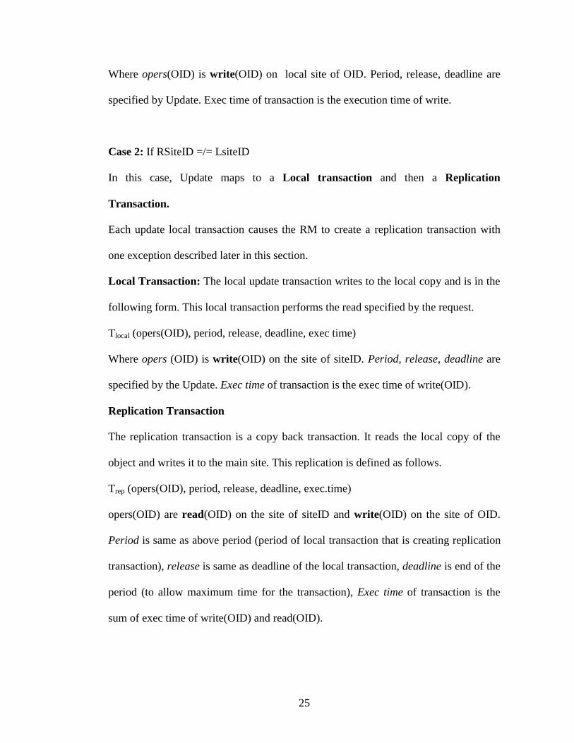
P4 r4 = 30 d = ? 38
Initially deadline is chosen as end of the period of Trep. In P2 d is changed to 4 as the
object becomes invalid after 14 on time line. Similarly in P3 d is changed to 2. Now d4
is 0, which is not possible. When Trep is released at 30 the object is not valid. So,
period cannot be 10. If it is 8, then the above problem does not occur. The same
example with period of Trep = 8 is explained below. The deadline is calculated as
follows.
Period Release Deadline Object valid until
P1 r1=0 d=8 14
P2 r2 = 8 d = 6 22
P3 r3 = 16 d = 6 30
P4 r4 = 24 d = 6 38
P5 r5 = 32 d = 6 46
. . .
. . .
P45 r45 = 360 d = 6 374
Initially deadline is chosen as end of the period of Trep. In P2 d is changed to 6 as the
object becomes invalid after 14 on time line. After this deadline remains constant.
Final deadline of Trep = 6. The example is shown for 360 units, because for every 360
seconds the above pattern repeats. 360 is the super period.
Example 2: This example shows that the requests always read the temporally
consistent data when JIT-RT replication algorithm is applied. The example illustrates

30
Case 2 of the proof of Theorem 1 in Section 4. That is when a new request is made at
Xi in the invalid interval, where OV<Xi<d
T(OID, period, release, deadline)
T1 (O1, 10, 7, 3), T2 (O1, 20, 17, 4), T3 (O1, 30, 27, 5)
Assume period of sensor update = 10. OV = 15 sec after every update. The deadline is
computed as follows.
Period Release Deadline Object valid until
P1=10 r1=0 d=10 15
P2=10 r2 = 10 d = 7 25
P3=10 r3 = 20 d = 7 35
P4=10 r4 = 30 d = 7 45
P5=10 r5 = 40 d = 7 55
. . .
. . .
In the above, d = 7 in P2 even though the object is invalid between 15 and 17. Because
there are no transactions, executing between 15 and 17. Similar is the case with other
deadlines.
3.2) Just In Time Real-Time Replication – Affected Set (JITRTR-AS):
JITRT-AS is the replication algorithm based on Affect Set Semantics. This algorithm
is applicable when a Request is made on the methods of the object rather than on
complete object. The basic idea here is similar to the idea of the JITRT-FO algorithm,

31
so this algorithm is based on the JITRT-FO algorithm. This section is organized as
follows. Section 3.2.1 gives the assumptions, Section 3.2.2 gives the system model,
and Section 3.2.3 describes the actual algorithm and the role of Replication Manager.
Section 3.2.4 explains the mapping of transactions to DASPCP model.
3.2.1) Assumptions: All the assumptions in the JITRT-FO algorithm are also the
assumptions in JITRT-AS algorithm except that attributes take the place of objects
here. Apart from those, there are some additional assumptions described below.
1) Replication Manager (RM) has special access to read() and write() operations for
each attribute. In this algorithm, RM replicates the attributes of the object instead
of full objects. This keeps the replication transaction independent from the method
requests.
2) The system may require run-time support for the replication of attributes.
3.2.2) System Model:
1) The distributed system consists of N sites.
2) Each object on local DB of each site is recognized by unique OID and also has the
following parameters:
Object - < OID, Attributes, Methods >
OID is unique object ID. Each attribute has its own value. Methods have set of reads
and writes on attributes of object with OID.
3) Each Attribute has the following parameters.
Attribute - <OID, Value, Time, AV >
32
OID is object identifier to which this attribute belongs; Value is the present value of
the attribute; AV is Attribute Validity of the Attribute.
4) Application Requirements are specified as method invocations with following
parameters:
Request (OID, Method, Period, release, deadline, LsiteID)
LsiteID is the site at which method request is originated. Here Request is made on the
method, whereas Request in JITRT-FO was made on the object.
3.2.3) Transaction Creation:
Given a system specified by the above model, JITRT-AS algorithm creates replication
transactions to ensure the availability of data like JITRT-FO. The algorithm produces
a model with two types of transactions, local transaction and replication transaction. A
transaction is a local transaction if all of its operations like read() and write(), execute
on the same site as the site on which request is made. A transaction is a replication
transaction if at least one of its operations executes on a remote site. Unlike JITRT-
FO replication, JITRT-AS replication creates replication transactions on the attributes
of an object rather on full object. So, JITRT-AS algorithm is similar to JITRT-FO
algorithm but the same thing what JITRT-FO algorithm does on object, is done on an
attribute of an object by JITRT-AS algorithm. If a request is made on method A that
has read affected set or write affected set {X, Y, Z}, then according to JITRT-AS
replication algorithm, three replication transactions are created, first transaction on X,
second on Y and third on Z.
Transaction model: The following are the parameters of the transaction.
33
Ttype < method(OID), period, release, deadline >
Where type is the type of transaction (local or replication), method is the method on
the which transaction takes place. The method has set of operations on attributes of
object OID.
For a request on a method, the replication transactions on the attributes (affected set of
the requested method) must be finished before the start of the local transaction so that
the local transaction can read the valid attributes copied on the local site by the
replication transactions. But this is going to be difficult as there is no specific order of
operations on attribute in a method. So, the basic idea is to keep replication
transactions independent from the method transactions.
Keeping this in mind request can be mapped to transactions.
3.2.4) Replication Manager:
The Replication Manager maps the requests to local and replication transactions. As
discussed above, JITRT-AS algorithm is similar to JITRT-FO algorithm but the same
thing what JITRT-FO algorithm does on object, is done on the attributes of an object
by the JITRT-AF algorithm. There are actually 2 cases. Case 1 occurs when site on
which requested method on OID is originally located is equal to the site at which
request is made and Case 2 occurs when site on which requested method on OID is
originally located is not equal to the site at which request is made.
Case1: If RSiteID == LsiteID
In this case a request maps to a local transaction with the following parameters,
Tlocal (method(OID), period, release, deadline)

34
Where method(OID) has set of opers(OID) to be executed on local site of OID,
opers(OID) can be reads and writes on the attributes of OID. Period, release, deadline
are specified by Request. The local transaction is simply an execution of the specified
method.
Case 2: If RSiteID =/= LsiteID
In this case a request maps to a replication transaction and a local transaction.
Replication transaction:
The replication transaction is created in a different way than that of the local
transaction. There are three steps in creating the replication transactions on the
attributes of an object.
i) The RM reads the Read Affected Set (RAS) and the Write Affected Set (WAS) of
the requested method from the specification. RAS of the method is the set of
attributes that a method reads and WAS of the method is the set of attributes that a
method writes [6].
ii) For each attribute in the RAS of the requested method, the RM creates a
replication transaction on that attribute according to the JITRT-FO replication
algorithm for requests. That is, calculate parameters of the replication transaction
according to JITRT-FO algorithm by replacing the object with the attribute. The
only difference between this algorithm and JITRT-FO is that, for each method, the
RM finds all the requests on that method and creates a replication transaction for
each attribute in that method. The deadline computation is based on the requests
on this method only. Here, if more than one method reads the same attribute then
35
each method separately creates a replication transaction on that attribute. For
example if method A and method B are reading the attribute X, then there will be
two separate replication transactions for X. First replication transaction on X is
based on all the requests on method A and second replication transaction is based
on all requests on method B. Since the attribute is replicated separately by each
method, this makes sure that all requests read the valid data.
iii) For each attribute in the WAS of the requested method, the RM creates a
replication transaction on that attribute according to the JITRT-FO algorithm for
updates.
Local Transaction: Following are the parameters for a local transaction.
Tlocal (Method(OID), period, release, deadline, exec time)
Where Method(OID) has set of opers(OID)on site of siteID. Opers(OID) can be reads
and writes on the attributes of OID. Period, release, deadline are specified by Request.
Exec time is the execution time of the method.

36
Chapter 4
Analysis
This chapter describes the analysis of the algorithms developed in chapter 3. Analysis
of the algorithms is done by stating and proving some theorems below for JITRT-FO
replication algorithm. Before proceeding to theorems we would like to define some of
the terms that will be used in the theorems.
Def 4.1) Temporal Consistency: In real-time databases data is not always permanent.
Sometimes the data is temporal, meaning the data becomes invalid (determined by the
application) after certain interval of time. The data is considered temporally consistent
at some point of time if it is valid at that point of time otherwise temporally
inconsistent.
4.1) Theorems:
Theorem 1: All requests will always access temporally consistent data.
Proof: Consider a replication transaction TO that copies object O. Let di be the
deadline of TO in its ith period as computed by JIT-RT replication algorithm. Let
OV be the point in time in the ith period after which the copy of object O becomes
invalid and let Pi be the period of TO.
O is temporally in consistent in the ith period in the interval between OV and d (see
figure below). This interval is known as the invalid interval (See Fig 4.1). Thus we
must prove that no request executes in the invalid interval.

37
Invalid Interval
|------------|-------------|---------|
Pi Pi+1
OV d
Figure 4.1 Invalid Interval 2
Recall from the JIT-RT replication algorithm that there are three possible cases
considered when the deadline of TO is computed (Section 3.1.3). We re-examine
those cases to prove that no request executes in the invalid interval.
Case 1) No requests execute in the invalid interval. Clearly, in this case no
requests read the invalid data.
Case 2) Some requests starts at time Xi such that OV < Xi < di. The JIT-RT
algorithm changes d to Xi, reducing the size of the invalid interval and making the
replication transaction finish before any requests read the data. Thus any such
requests will read valid data in this case.
Case 3) Some requests execute throughout the invalid interval. In this case, some
requests start before or at OV and finishes at or after deadline, d, then the JIT-RT
replication algorithm computes d to be OV. By doing this, we are removing the
invalid interval. Thus all the requests read the valid data.
In all the cases, we have proved that the requests read the valid data. Thus all
requests always read temporally consistent data.

38
Theorem 2: The period of TO must be in phase and equal to the period of sensor
update transaction for object O in order for all requests to read valid data using
our algorithm.
Proof: To prove that the period of replication transaction and the period of sensor
update must be in phase, let us consider a contradictory situation; assume they are not
in phase. i.e. assume periods PTo for replication transaction TO and for PSUo for sensor
update trasanction SUO are not in phase. This implies that the two above periods are
not equal (If the two periods are equal, then they are always in phase).
Here we consider the two cases. One is that PTo > PSuo and the second case is PTo <
PSuo. We prove that it is not possible to construct a replication transaction with the
above two cases. We also prove that when both the periods are equal and all requests
intuitively read valid data.
Case 1: PTo > PSuo:
As discussed in Theorem 1, the object is invalid only in the invalid interval and the
deadline of TO can be changed to OV according to Theorem 1. Now consider the
calculations of deadlines (di) in each period of replication transaction.
Initially d = end of the first period. In each successive period, deadline is calculated
based on whether there are any requests in the invalid interval. The minimum deadline
in any period is OV. So, once the deadline in any period becomes OV then the
calculation of deadline is stopped and the final deadline is taken as OV. It can be
observed from the Fig 4.2 below that, as i increases, since PTo > PSuo, d decreases and
at some point (for some ‘i’), d becomes 0 or less than 0.

39
|--------|--------|--------|--------|--------|--------|--------|--------|--------| (SUO)
P1 P2 P3 P4 P5 P6 P7 P8 P9 P10
OV2 OV3 OV4 OV5 OV6
Ä----d1----> Ä--d2-Å Äd3-> <d4> d5=?
|-----------|-----------|----------|----------|-----------|-----------| (TO)
P1 P2 P3 P4 P5 P6 P7
Figure 4.2 - Deadline Assignment 1
Thus we cannot guarantee that all the requests will read the valid data all the time.
Case 2: PTo < PSuo:
From the figure 4.3, it can be observed that, since both the periods are not in phase,
there may be a case (d4 in figure 4.3) where we cannot choose a deadline that will
satisfy all requests reading valid data.
|--------|--------|--------|--------|--------|--------| (SUO)
P1 P2 P3 P4 P5 P6 P7
OV2 OV3 OV4 OV5 OV6
Ä--d1-><d2> Äd3--> d4=?
|------|------|------|------|------|------|------| (TO)
P1 P2 P3 P4 P5 P6 P7
Figure 4.3 - Deadline Assignment 2
In the second case also we cannot guarantee that a requests will always read the valid
data.
Now let us see how it is intuitive that if PTo = PSuo, we do not come across the
problem of deadline becoming 0. It can be observed from Fig 4.4 that, between the
start of every TO and OVi there is always some constant time (as shown in figure 4.4),
which means they do not coincide at any time. So, deadline can never be 0 in this case

40
and all the requests read the valid data (because deadline assignment is according to
JIT-RT algorithm).
|--------|--------|--------|--------|--------|--------|--------|--------|--------| (SUO)
P1 P2 P3 P4 P5 P6 P7 P8 P9 P10
OV2 OV3 OV4 OV5 OV6
Äd1-Å Äd2-Å Äd3--Å Ä-d4-Å Äd5-Å
|--------|--------|--------|--------|--------|--------| (TO)
P1 P2 P3 P4 P5 P6 P7
d2 = d3 = d4 =….=constant =/= 0
Figure 4.4 Deadline Assignment 3
Thus it is proved that the period of TO must be in phase and equal to the period of
sensor update transaction for object O in order for all requests to read valid data.
Theorem 3: The deadline assignment, according to the JITRT algorithm, is
necessary and sufficient for ensuring the temporal consistency of data.
Proof:
Sufficient condition: Theorem 1 proves that the data objects read by all the requests
are always temporally consistent, which means that the deadline assignment is
sufficient for ensuring the temporal consistency of data.
Necessary Condition:
Theorem 1 considers all the three cases while computing the deadline and proves that
all the requests always read the valid data.
To prove that the deadline assignment of replication transaction, TO, according to our
algorithm is necessary, lets us take the contradictory situation. That is let us assume

41
there exists a deadline assignment of a replication transaction by some algorithm,
other than JITRT algorithm, greater than the deadline assigned by JITRT algorithm.
As discussed above, the object is invalid in ith period only in the invalid interval. The
minimum deadline assigned by JITRT algorithm is OV in ith period. If there exists a
deadline of TO > OV, then there exists some invalid interval between OV and d, in
which the transactions executing in this interval read invalid data, which contradicts
the definition of temporal consistency in real-time systems. So, any assignment of
deadline is always less than or equal to the deadline assigned by our algorithm.
This implies that the deadline assignment by our algorithm is a necessary condition to
ensure the temporal consistency of data read by the transactions.
Even though the above theorems are proved for JITRT-FO replication algorithm, they
are also true for JITRT-AS algorithm. This is intuitive because, JITRT-AS algorithm
is similar to JITRT-FO algorithm except that JITRT-FO algorithm replicates the full
object whereas JITRT-AS algorithm replicates the attributes of the object. All the
method requests also read the valid attributes, as the attributes are replicated according
to JITRT-FO algorithm by replacing object with the attributes of the object. As far as
Theorem 2 is concerned, the period of the replication transaction on an attribute of
object O, TO must be in phase and equal to the period of sensor update transaction for
the same attribute of object O in order for all requests to read valid data.
42
Chapter 5
Implementation Methodology:
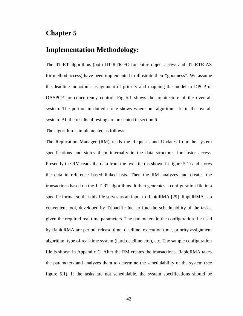
The JIT-RT algorithms (both JIT-RTR-FO for entire object access and JIT-RTR-AS
for method access) have been implemented to illustrate their “goodness”. We assume
the deadline-monotonic assignment of priority and mapping the model to DPCP or
DASPCP for concurrency control. Fig 5.1 shows the architecture of the over all
system. The portion in dotted circle shows where our algorithms fit in the overall
system. All the results of testing are presented in section 6.
The algorithm is implemented as follows:
The Replication Manager (RM) reads the Requests and Updates from the system
specifications and stores them internally in the data structures for faster access.
Presently the RM reads the data from the text file (as shown in figure 5.1) and stores
the data in reference based linked lists. Then the RM analyzes and creates the
transactions based on the JIT-RT algorithms. It then generates a configuration file in a
specific format so that this file serves as an input to RapidRMA [29]. RapidRMA is a
convenient tool, developed by Tripacific Inc, to find the schedulability of the tasks,
given the required real time parameters. The parameters in the configuration file used
by RapidRMA are period, release time, deadline, execution time, priority assignment
algorithm, type of real-time system (hard deadline etc.), etc. The sample configuration
file is shown in Appendix C. After the RM creates the transactions, RapidRMA takes
the parameters and analyzes them to determine the schedulability of the system (see
figure 5.1). If the tasks are not schedulable, the system specifications should be

43
changed (input file should be modified) and the modified data is inputted to RM again
until the tasks are schedulable. If the tasks are found to be schedulable, RapidRMA
generates a configuration file, which serves as input to the scheduling service. The
scheduling service reads the configuration file generated by RapidRMA and schedules
the transactions and runs, for example, on a RT-CORBA server.
Offline
Run-TimeSyste
m
Figure 5.1 - System Execution
SystemSpecifications
JIT-RT-FOor
JIT-RT-ASConfig File
SchedulabilityAnalysis
Tool
Config FileSpecifies DPCP or DASPCPmodel, priorities etc
SchedulingService
Not schedulable
DB
Site 1
DB
Site n
Schedule
Assign priorities
Runtime System
Replication

44
Chapter 6
Testing
This section presents the tests that were performed and the results obtained for each
test. We performed the test suites that compared our algorithm with two replication
strategies. The first strategy, called Full Rep, produces full replication in which all the
objects are replicated on all the sites and the second strategy, called No Rep, is with no
replication in which the request on a remote object will execute a remote transaction.
6.1) Test Generation:
Figure 6.1 depicts the generation of tests. A Generator class has been created that
creates the objects, requests, sensor updates, updates randomly and writes them into a
text file that serves as an input to Replication Manager. A Driver class runs the
Generator that actually creates an input file and then runs the
ReplicationManager. The RM executes the algorithm and creates the
transactions according to JITRT algorithm (for both Full Object and for Affected Set)
and writes the results into two separate files. These files are used as input files to a
schedulability tool like RapidRMA [29]. The ReplicationManager also takes the
requests and updates from the same input file created by the Generator and creates
the transactions using Full Rep and No Rep strategies and writes the results to separate
files.
In each of the test we performed, we specified the execution time for read to be 1 unit
and execution time for write to be 2 units. One unit of the network delay is added to
the remote transactions.

45
Figure 6.1 – Test Generation
6.2) Performance measures:
The performance measures we used are of two types. The first measure is the system
schedulability percentage and second measure is the task schedulability percentage.
System schedulability measures the overall schedulability of the system, in which all
the tasks in all nodes are schedulable. Task schedulability measures the schedulability
of the tasks in the system. So if the system is not schedulable, task schedulability
shows how close the system is to being schedulable. We have chosen system
schedulability percentage measure, because our system is hard-deadline real-time
system in which the system becomes un-schedulable even if a single task is un-
schedulable. We have chosen task schedulability percentage measure, because this
measure shows how close the system is towards the schedulability.
In each test suite, we have compared the results of JITRT-FO with the results obtained
with NoRep and FullRep algorithms. The results of each test are averaged from 15
trials. We have chosen 15 trials because we found this number to be optimal after
doing statistical analysis to find out the error % with this number of trials. We have
ReplicationManagergenerates
GeneratorInput File
JITRT
No Replication
Full Replication
generates
Output files

46
done the analysis using Statistical Analysis Software (SAS) and found the error % to
be less than 5%, which is reasonably acceptable.
6.3) JITRT-FO Testing
6.3.1) Test Suites:
Initially testing is performed for baseline test. Next the testing is performed on three
other test suites by changing one of the parameter ranges in each test suite. This
section explains in details how the base case and the three test suites are performed.
6.3.1.1) Baseline Testing:
The base case testing is done using the parameter ranges shown in Table 6.1. The
Driver class runs the Generator and the ReplicationManager 15 times (15 trials) for the
base case and creates separate output files for each trial. Once all the files are created
RapidRMA is run on these files to find the schedulability of the system for each trial.
Then the percentage of the schedulability of the system for JITRT replication, NoRep
and FullRep algorithms are compared and tabulated.
Parameter RangePeriod 150 – 400
No of Objects 7 – 12No of sites 5 – 12
No of Reqs/Object 3 – 6percentage of Updates 50
Table 6.1 Parameter Ranges for Baseline Testing (JITRT-FO)
In table 6.1, we have chosen the period to be between 150 and 400, because this range
best showed the differences among the results using three strategies. Choosing above
400 gave lot of leeway for the schedulability and we found the schedulability using
three strategies (JITRT replication, NoRep and FullRep) to be more than 90%. This

47
does not illustrate any goodness of the JITRT replication algorithm. Choosing period
less than 150 gave schedulability below 30% for all three strategies. For similar
reason, the number of objects is chosen to be between 7 and 12, number of sites is
chosen between 5 and 12 and number of requests is chosen to be between 3 and 6 and
percentage of updates is chosen to be 50. The percentage of updates denotes the
percentage of updates from the sum of number of updates and requests. The results are
shown in Section 6.3.2.
6.3.1.2) Test Suite 1 – Effect of Period
This test is performed to show the effect of period on the schedulability of transactions
executed by our algorithm. This test suite actually performs the tests with three
different ranges of periods keeping all the ranges of other parameters same as the
above base case. The three different ranges of the period are chosen such that the
results clearly illustrate the goodness of the JITRT-FO algorithm.
The three ranges of period are given in table 6.2.
Short 100 – 250
Medium 250 – 350
Long 400 – 600
Table 6.2 Ranges of Period for Test Suite 1
6.3.1.3) Test Suite 2 – Effect of Number of Objects
This test is performed to show the effect of number of objects on the schedulability.
This test suite actually performs the tests with three different ranges of number of

48
objects keeping all the ranges of other parameters same as the above base case. The
two different ranges of the number of objects are chosen to be less than, greater than
the range of number of objects in base case. The third range is chosen to be similar but
not the same as the range of number of objects in the base case.
The three ranges for number of objects are given in table 6.2.
Short 2 – 7
Medium 7 – 10
Long 10 – 16
Table 6.3 Ranges of number of objects for Test Suite 2
6.3.1.4) Test Suite 3 – Effect of Percentage of Updates
This test is performed to show the effect of percentage of updates, with respect to total
number of transactions, on the schedulability. This test suite actually performs the
tests with three different values for percentage of updates keeping all the ranges of
other parameters same as the base case.
The three values of update percentages are given in table 6.4.
Short 0
Medium 45
Long 100
Table 6.4 value of percentage of updates for Test Suite 3

49
6.3.2) Results
This section explains the results obtained in each test suite described above, including
baseline testing.
6.3.2.1) Baseline Testing: The schedulability of the system for the three strategies is
shown in Figure 6.2. It can be observed that the schedulability percentage for FullRep
algorithm is always less than that for JITRT replication. This is because FullRep
algorithm consists of more transactions in the system than the other two replication
strategies, for the same requests and updates.
80%87%
53%
0%10%20%30%40%50%60%70%80%90%
100%
JITRT-FO NoRep FullRep
Sch
ed %
Figure 6.2 – System Schedulability for Baseline Testing
It is found that the schedulability percentage for NoRep is found to be slightly more
than that for JITRT replication. This is because the NoRep algorithm has fewer
transactions than the JITRT-FO algorithm because JITRT-FO creates a replication
transaction for each update. However the JITRT replication guarantees that the
objects read by the requests are always valid whereas NoRep does not guarantee

50
temporal consistency. That is, even if the data on the remote site may be valid at the
time it reads, it may become invalid within the period of network delay.
We have also compared the results using task schedulability percentage. The results
(Figure 6.3) were found to be similar to the system schedulability percentage. High
percentage schedulability for JITRT-FO and NoRep shows that the system, even if it
is not schedulable, is nearer to schedulability.
JITRT-FO Results for Base Case (Task Sched)
93%99%
80%
0%
20%
40%
60%
80%
100%
JITRT-FO NoRep FullRep
Sch
ed %
Figure 6.3 – Task Schedulability for Baseline Testing
6.3.2.2) Test Suite1 – Effect of Period: The results for test suite 1 are explained in
this section. This test suite illustrates the effect of period on the results. The results for
all three ranges are shown in Figure 6.4. System schedulability percentage for all three
strategies is found to be less than that for base case. As we expected, the figure
illustrates that increase in the period increased the schedulability percentage of the
system.
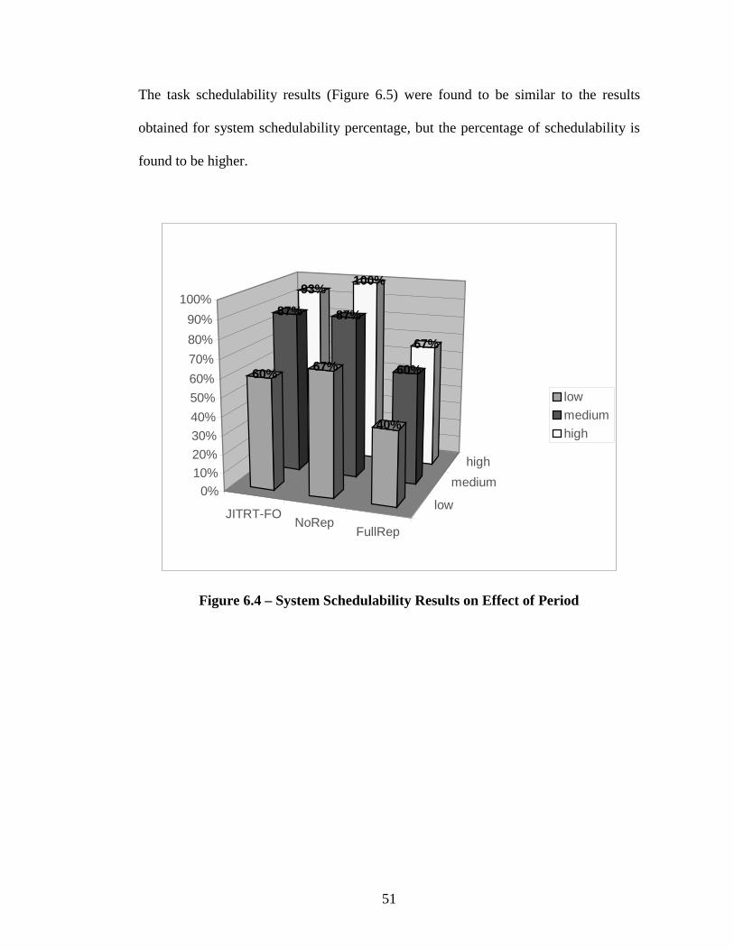
51
The task schedulability results (Figure 6.5) were found to be similar to the results
obtained for system schedulability percentage, but the percentage of schedulability is
found to be higher.
JITRT-FONoRep
FullRep
low
medium
high
93%100%
67%
87% 87%
60%60% 67%
40%
0%10%
20%
30%
40%
50%
60%
70%
80%
90%
100%
low
medium
high
Figure 6.4 – System Schedulability Results on Effect of Period

52
JIT
RT
-FO
NoR
ep
Ful
lRep
lowmedium
high
99% 100% 97%98% 99%93%
78% 85%
62%
0%
20%
40%
60%
80%
100%
Sch
ed%
lowmediumhigh
Figure 6.5 – Task Schedulability Results on Effect of Period
6.3.2.3) Test Suite2 – Effect of Number of Objects: The results for test suite 2 are
explained in this section. This test is performed to illustrate the effect of number of
objects on the system schedulability.
The results for all three ranges are shown in Figure 6.6. In general we found that
decrease in the number of objects increased the schedulability percentage of the
system, because decreasing the number of objects decreases the number of
transactions.

53
JIT
RT
-FO
NoR
ep
Ful
lRep
high
low
93%100%
73%80% 80%
47%
60%67%
27%
0%10%20%30%40%50%60%70%80%90%
100%
Sch
ed %
highmediumlow
Figure 6.6 – System Schedulability Results on No of objects
Figure 6.7 details the results obtained for task schedulability. All the results look
similar to that of system schedulability but the task schedulability percentage for each
case is higher than that for system schedulability percentage.
JIT
RT
-FO
NoR
ep
Ful
lRep
highmedium
low
100% 100%96%96% 98%
84%76% 82%
56%
0%
20%
40%
60%
80%
100%
Sch
ed
%
highmediumlow
Figure 6.7 – Task Schedulability Results on Effect of No of objects

54
6.3.2.4) Test Suite3 – Effect of Update percentage: The results for test suite 3 are
explained in this section. This test suite is chosen to illustrate the effect of update
percentage on the system schedulability. The system schedulability results for all three
ranges are shown in Figure 6.8.
In general we found that that the decrease in the update percentage increased the
schedulability percentage of the system. This is true, because updates are more costly
than requests and each update creates a new replication transaction in JITRT-FO
algorithm. Increase in the update percentage decreased the schedulability percentage
of the system, which is as expected.
Figure 6.9 details the results obtained for task schedulability. All the results look
similar to that of system schedulability but the task schedulability percentage for each
case is higher than that for system schedulability percentage.
JITRT-FO
NoRepFullRep
high
mediumlow
93% 100%
67%
80% 80%
47%
60%
73%
47%
0%10%20%30%40%50%60%70%80%90%
100%
Sch
ed %
highmediumlow
Figure 6.8 – System Schedulability Results on effect of update percentage
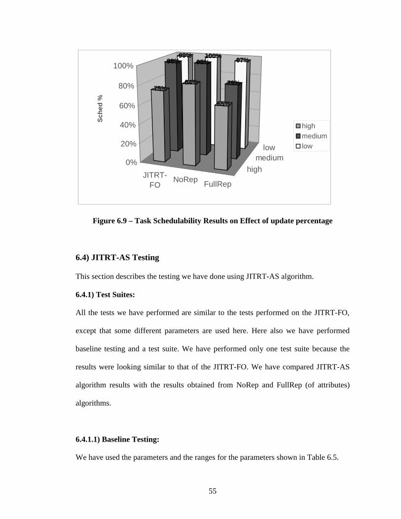
55
JITRT-FO
NoRepFullRep
high
mediumlow
99% 100%97%98% 98%
79%75%
84%
65%
0%
20%
40%
60%
80%
100%
Sch
ed %
highmediumlow
Figure 6.9 – Task Schedulability Results on Effect of update percentage
6.4) JITRT-AS Testing
This section describes the testing we have done using JITRT-AS algorithm.
6.4.1) Test Suites:
All the tests we have performed are similar to the tests performed on the JITRT-FO,
except that some different parameters are used here. Here also we have performed
baseline testing and a test suite. We have performed only one test suite because the
results were looking similar to that of the JITRT-FO. We have compared JITRT-AS
algorithm results with the results obtained from NoRep and FullRep (of attributes)
algorithms.
6.4.1.1) Baseline Testing:
We have used the parameters and the ranges for the parameters shown in Table 6.5.

56
Parameter RangePeriod 150 – 400
No of Sites 7-10No of objects 6 – 12No of Reqs 3 – 6
No of Attributes 5 – 9RAS 2 – 5WAS 1 – 3
No of Methods 3 – 6
Table 6.5 Parameter ranges for baseline testing (JITRT-AS)
The baseline testing was performed similar to the baseline testing in JITRT-FO. We
have used the results obtained for NoRep algorithm and FullRep (of attributes)
algorithm to compare with JITRT-AS algorithm. We have chosen the above ranges,
because the results obtained with these ranges illustrate the goodness of JITRT-AS
algorithm. The results for baseline testing and other three strategies are shown in
Section 6.4.2.
6.4.1.2) Test Suite 1 – Effect of WAS
This test is performed to show the effect of WAS, on the schedulability of transactions
executed by our algorithm. This test suite actually performs the tests with three
different ranges (see Table 6.6) of WAS keeping all the ranges of other parameters
same as the above base case. The three different ranges for WAS are chosen such that
the results clearly illustrate difference in the schedulability percentage.

57
Short 100 – 250
Medium 250 – 350
Long 400 – 600
Table 6.6 – Ranges of WAS for test suite 1
6.4.2) Results
6.4.2.1) Baseline Testing:
The results obtained for baseline testing are shown in Figure 6.10. It is found that the
schedulability percentage for NoRep is found to be 87%, which is slightly more than
that for JITRT replication (73% schedulability) but JITRT replication guarantees that
the objects read by the requests are valid when needed, where as no replication
algorithm does not guarantee temporal consistency of data when needed. It is also
found that the schedulability percentage for JITRT-AS algorithm is significantly
greater than the schedulability percentage for full replication algorithm (53%).
73%
87%
53%
0%
10%
20%
30%
40%
50%
60%
70%
80%
90%
100%
JITRT-AS NoRep FullRep
Sch
ed %
Figure 6.10 – System Schedulability for Baseline Testing
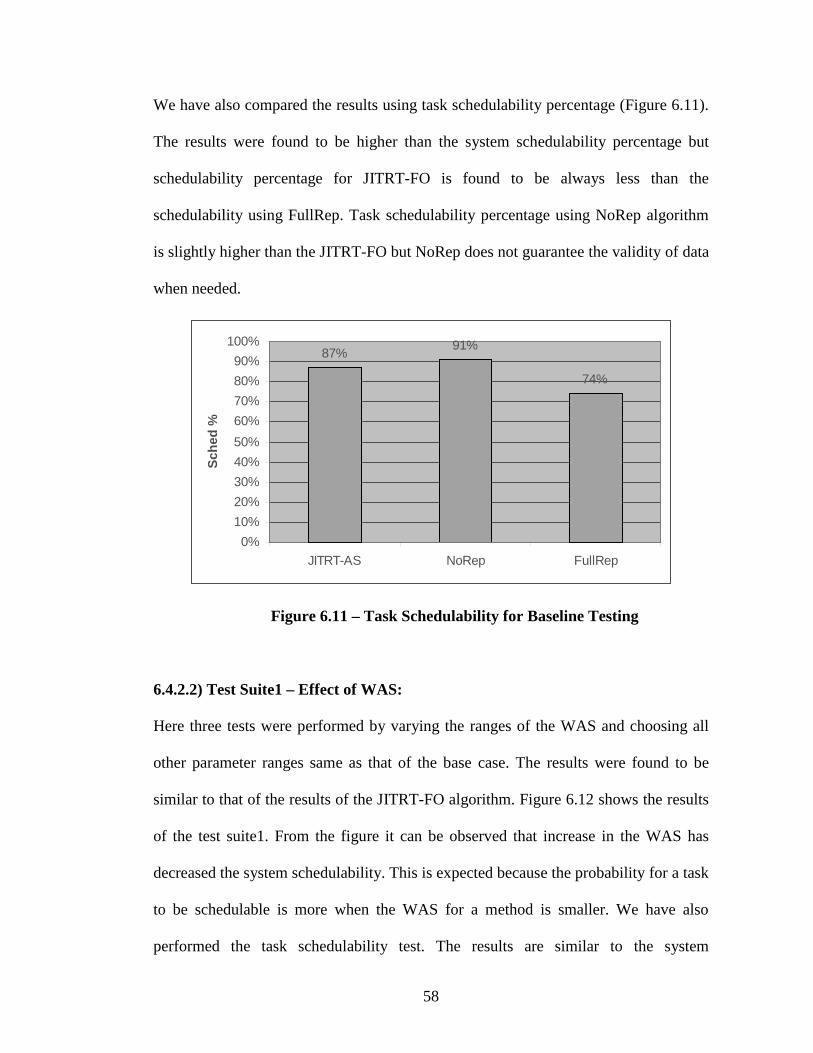
58
We have also compared the results using task schedulability percentage (Figure 6.11).
The results were found to be higher than the system schedulability percentage but
schedulability percentage for JITRT-FO is found to be always less than the
schedulability using FullRep. Task schedulability percentage using NoRep algorithm
is slightly higher than the JITRT-FO but NoRep does not guarantee the validity of data
when needed.
87%91%
74%
0%
10%
20%
30%
40%
50%
60%
70%
80%
90%
100%
JITRT-AS NoRep FullRep
Sch
ed %
Figure 6.11 – Task Schedulability for Baseline Testing
6.4.2.2) Test Suite1 – Effect of WAS:
Here three tests were performed by varying the ranges of the WAS and choosing all
other parameter ranges same as that of the base case. The results were found to be
similar to that of the results of the JITRT-FO algorithm. Figure 6.12 shows the results
of the test suite1. From the figure it can be observed that increase in the WAS has
decreased the system schedulability. This is expected because the probability for a task
to be schedulable is more when the WAS for a method is smaller. We have also
performed the task schedulability test. The results are similar to the system
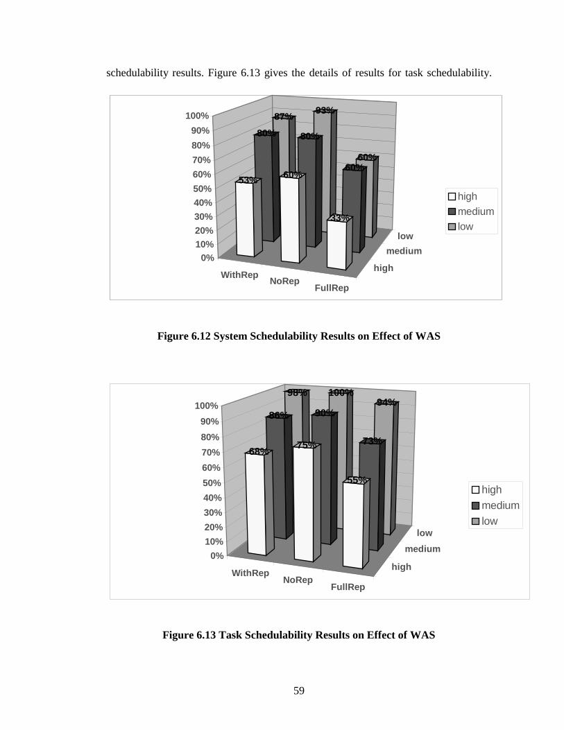
59
schedulability results. Figure 6.13 gives the details of results for task schedulability.
WithRepNoRep
FullRep
high
medium
low
87%93%
60%
80% 80%
60%53% 60%
33%
0%10%20%
30%
40%
50%
60%
70%
80%
90%
100%
high
medium
low
Figure 6.12 System Schedulability Results on Effect of WAS
WithRepNoRep
FullRep
high
medium
low
98% 100%94%
86% 90%
73%68%
75%
55%
0%
10%
20%
30%
40%
50%
60%
70%
80%
90%
100%
high
medium
low
Figure 6.13 Task Schedulability Results on Effect of WAS

60
6.5) Effect of number of remote requests and updates on JITRT-FO
This section describes the testing performed to show the effect of number of remote
transactions on the algorithm. Till now all the tests have shown that the schedulability
% for NoRep is slightly more than the JITRT algorithm. This test shows that JITRT-
FO algorithm is better than the NoRep algorithm when there are more remote requests
or updates. The following are the results obtained with all the parameters same as
baseline testing for JITRT-FO except that all the requests are remote requests. The
results shows that the schedulability % of JITRT-FO is 80%, which is reasonably high
compared to 60% schedulability for NoRep algorithm. This shows that JITRT-FO
algorithm plays an important role when there are more remote transactions.
Figure 6.14 Test with all remote requests (JITRT-FO)
80%87%
53%
0%10%20%30%40%50%60%70%80%90%
100%
JITRT-FO NoRep FullRep
Sch
ed %

61
Chapter 7
Conclusion
This chapter discusses the conclusion of the thesis work. We have developed two
versions of the replication algorithm that does replication in distributed real-time
object-oriented databases. The first version, called JITRT-FO, is based on requests
made on the full object and the second version, called JITRT-AS, is based on requests
made on the methods of an object. We have also proven that replication of data
according to the JITRT algorithms makes the requests read valid data when needed.
We have implemented the algorithms on a full object and on affected sets and we have
performed some tests to indicate the goodness of the algorithms. The results of the
tests performed on the JITRT algorithm were compared with the results obtained with
no replication and with full replication. The results showed that the percentage
schedulability of the system with our algorithm is better than the percentage
schedulability with the full replication algorithm. Even though the percentage
schedulability of the system with our algorithm is usually less than the percentage
schedulability of the system with the no replication algorithm, the no replication
algorithm does not guarantee that all requests read valid data when needed, while ours
does. This is crucial in the kinds of real-time applications for which our algorithms
were designed.
The JITRT algorithm that we have developed plays an important role in distributed
hard real-time applications where the validity of data is important, because our

62
algorithm performs replication only when and where needed. This reduces the
overhead on the system and makes the data available locally.
63
Chapter 8
Future Work
While the JITRT algorithm provides a good technique of replicating the data in
distributed real-time systems, there is further work that can be done to enhance the
current research, and to extend it to other areas.
1) Dynamic case: The present algorithm is designed for static system in which all
the requests, number of sites and number of objects are known a priori and will
not change once the system starts executing. Considering and developing the
replication algorithm for the dynamic case in which the requests can come
when the system is running, would be more challenging because the algorithm
needs to change the strategy when the requests come and go at runtime.
2) Heterogeneous Databases: Currently the algorithm assumes that the system
has all the DBMS same. It would be interesting to consider that each site has a
different DBMS, because the replication methodology may be different at
different DBMS and communication of one DBMS with other becomes more
complex.
3) Multiple Objects: It would be interesting to see how the algorithm works by
relaxing some assumptions like each object may be originated from more than
one site. The replication algorithm can copy the object that is nearer to the
requesting site. This reduces the network delay.
4) Real Data: We have presently tested the algorithm with the dummy data. So it
would be interesting to test the performance of the algorithm with the real data.
64
5) Concurrency control protocols: Presently our algorithm is modeled to fit
with DPCP and DASPCP, but it would be interesting to see how it can be
mapped to other concurrency control protocols.
6) Real Transactions: Instead of using just requests and updates, one can use the
real transactions and design the algorithm.
65
References:
1) Shin K. and P. Ramanathan. “Real-Time Computing: A New Discipline of
Computer Science and Engineering”. Proceedings of IEEE 82, Special Issue
on Real-Time Systems, 6-24 (1994).
2) Sang H Son, Robert C. Beckinger, and David A. Baker. “DRDB: Towards
Distributed Real-Time Database Services for Time-Critical Active
Applications” Journal of Systems and Software, Special Issue on Real-Time
Active Database Systems, vol. 42, pp. 193-204, 1998.
3) Krithi Ramamrutham. “Real-Time Databases”. International Journal of
Distributed and Parallel Databases, February 28,1996.
4) IEEE Real-Time Technology and Applications Symposium, Montreal, Canada,
June 1997.
5) International Workshop on Real-Time Database Systems, Burlington,
Vermont, September 1997.
6) Lisa Cingiser Dipippo, Victor Fay Wolfe, Levon Esibov, Michael Squadrito,
Gregory Cooper, Bhavani Thuraisingham, Peter Krupp, Michael Milligan,
Russel Johnston, Ramachandra Bethmangalkar. “The Affected Set Priority
Ceiling Protocols for Real-Time Object-Oriented Concurrency Control”.
International Journal of Computer Systems Science and Engineering, Vol. 14,
1999.
7) Sha L., Raghunathan Rajkumar, and Lehoczky Z. “Priority Inheritance
Protocols: An approach to Real-Time Synchronization”. IEEE Transactions on
computers, pp. 1175-1185, 1990.
66
8) Abbott R., Garcia-Molina H, and B. Kao. “Scheduling Real-Time
Transactions: A Performance Evaluation”. ACM Transaction. On Database
Systems 17 (3), 513-560 1992.
9) Son, S.H, F. Zhang, and B. Hwang. “Concurrency Control for Replicated Data
in Distributed Real-Time Systems”. Journal of Database Management 7,
Special Issue on Real-Time Database Systems: Theory and Practice. 12-23,
(1996).
10) Ramez Navathe and Shamkant Elmashri. “Fundamentals of Database
Systems”. Third edition, 1999.
11) Song X. and J.W.S. Liu. “How Well Can Data Temporal Consistency be
Maintained?”. Proceedings of the IEEE Symposium on Computer-Aided
Control Sytstems Design, 1992.
12) Audsley N, Burns A, Richradson M., and Wellings A. “A Database Model for
Hard Real-Time Systems”. Technical Report, Real-Time Systems Group,
University of York, U.K.
13) Harista J. R., VaCarey M. J. and Livny M. “Dynamic Real-Time Optimistic
Concurrency Control”. Proceedings of Real-Time Systems Symposium, Dec.
1990.
14) Son S. H.. “Replicated Data Management in Distributed Database Systems”.
Vol. 17, SIGMOD RECORD, Dec-1998.
15) Ozsu and Valduriez.“Distributed Databases”. 1999.
16) Michael Stonebraker and Joseph M. Hellerstein. “Readings in Database
Systems” 3rd edition.

67
17) Raghu Ramakrishnan and Johannes Gehrke. “Database Management Systems”
2nd Edition, 2000.
18) Sang H. Son and Spiros Kouloumbis. “A Token Based Synchronization Scheme
For Distributed Real-Time Databases”. Information Systems, Vol 18, 1993.
19) Sang H. Son. “Synchronization of Replicated Data in Distributed Systems”.
Inform Systems Vol. 12, No. 2 pp. 191-202, 1987.
20) Robert H. Thomas “A majority Consensus Approach To Concurrency Control
for Multiple Copy Databases”. ACM Transactions on Database Systems 4(2),
180-209 (1979).
21) J. Huang, J. A. Stankovic, K. Ramamritham, D. Towsley. “Experiment
Evaluation of Real-Time Optimistic Concurrency Control Schemes”.
Proceedings of 17th International Conference on very large databases,
Barcelona, September-1991.
22) M. Carey, and M. Livny. “Conflict reduction tradeoffs for replicated data”.
IEEE Transactions on knowledge and Data Engineering, Vol 2, No. 2, June
1990.
23) Ming Xiong, K. Ramamritham, J. Harista, J. A. Stankovic. “MIRROR: A State
Consious Concurrency-Control Protocol for Replicated Real-Time Databases”
Workshop on Advanced Issues of E-Commerce and Web/based Information
Systems, 1998.
24) Jane W.S. Liu. “Real-Time Systems”. Prentice Hall, 2000.
68
25) Bhaskar Purimetla, Rajendran M. Sivasankaran, Krithi Ramamritham and John
A Stankovic. “Real-Time Databases: Issues and Applications” in Principles of
Real-Time Systems, Sang Son, Ed. Prentice-Hall, 1994.
26) http://www.dedicated-systems.com/encyc/techno/terms/defini/def.htm
(Date Accessed: 02-15-2001)
27) Lui Sha, Mark H. Klein, John B. Goodenough “Rate Monotonic Analysis for
Real-Time Systems” Kluwer Academic Publishers, March 1991.
28) http://www.dedicated-systems.com/encyc/publications/faq/rtfaq.htm (Date
Accessed: 02-15-2001)
29) http://www.tripac.com (Date Accessed: 11-15-2000)
30) Lisa DiPippo , V. F. Wolfe, R. Ginis, M. Squadrito, T. Wheeler “A Scheduling
Service for a Dynamic Real-Time CORBA System ” Proceedings of The
Twenty-Second Annual International Computer Software and Application
Conference, August 1998.
31) Victor Fay Wolfe, Lisa Cingiser DiPippo, Roman Ginis, Michael Squadrito,
Steven Wohlever, Igor Zykh and Russell Johnston. “Expressing and Enforcing
Timing Constraints in a Dynamic Real-time CORBA System” pp 253-280, Vol.
16, Real-Time Systems, May 1999.

69
Appendix A:
Implementation details of JITRT-FO:
The details of the implementation of the JITRT-FO replication algorithm are discussed
in this section. The implementation details involve the implementation of the
Replication Manager (RM), which does the majority of the work involved in the
algorithm and many other classes that are used by RM.
Overview of this implementation:
The implementation can be summarized as follows:
Replication Manager (RM) takes the parameters of the Requests and Updates from
system specifications (in our case they are text files). RM also reads the list of sites
and the objects, the location of each object (original copy), sensor update parameters
from the different text files. RM then analyzes the parameters of the requests and
updates and creates local transactions on each site for each object, and all required
replication transactions on each site. After creating all the transactions, RM sends the
transactions parameters into a configuration file in a specific format. This file is
actually an input to Rapid RMA that does the schedulability analysis of the created
transactions.
RM uses many classes to do the above task. Each class is explained in the next sub-
section.
Detailed Explanation:
Input File:
Following is format for the input file used by the Replication Manager.

70
This file consists of all the Required parameters in the below format. Each line
represents a separate data. The file has different sections.
Assumptions:
1) Each set of parameters are separated by the line that has * on it.
2) Commented line should start with #
3) The first field should always be in the ascending order.
The first part represents the set of objects that are participating in the system. The data
format for this is (OID, value, time, OV). Order of OID is 1,2,3,4…..
The next part is the set of sites present in the system. This data consists of list of
siteID’s used by requests and updates. Order of siteID is 1,2,3….
The next section consists of list of OID and the siteID at which each object is located.
Format is (OID, siteID). The order of the OID should be 1,2,3…..
The next section lists the sensor updates for each object. The format of the
parameters is (OID, period, release, deadline). The list should be in the ascending
order of OID.
The next set of data lists the requests with the format (OID, period, release, deadline,
siteID).
Here release should always be > (OV + release of sensor transaction on object OID).
So, when entering the parameters in the file, it is the users responsibility to check this
condition. Requests should be in the increasing order of OID. SiteID and OID used
should be present in the above given lists of objects and sites.
The last section consists of the list of all update parameters in the format shown
below. (OID, period, release, deadline, siteID)

71
Each line represents an update.
Classes: Class Replication Manager uses number of other classes to create the
transactions and generate a configuration file. The detailed explanation of each class is
given below.
1) ListReferenceBased: This class is reference based linked list that can
store the list of Objects of type Object. This has many public and private
methods. Method get(int x) retrieves element at index x. isEmpty() returns
true if the list is empty else returns false. size() returns the present size of
the list. add(Object x) adds the object at the end of the
list.
2) Node: The above class uses this class. Node represents a node in the list. This
actually stores the object and has the pointer to the next Node.
3) ListOutOfBoundException: This is a java Exception class. This is
thrown when the user tries to access an object that is not there in the list.
4) RequestParameters: This class has the public attributes in each attribute
is a parameter of each request. RM reads parameters of each request from file
and creates an instantiates an object that stores these parameters. So, each
instance represents a request here. This class has two constructors (default
constructor and the constructor that initializes the attributes specified by
arguments).
5) UpdateParameters: This class is very similar to RequestParameters but
this stores the attributes of the Updates instead of Requests. The parameters are
read from the input file.

72
6) RTObject: This class represents a real-time object. This has 4 attributes
(OID, value, time, OV) that are the attributes of an RT object. value
is the value of the object at time. OV is the object validity of the RT object after
which the object’s value becomes invalid.
7) RTTransaction: This class represents a real-time transaction. RM uses this
when creating the transactions (local and replication). This class has attributes
(transID, OID, type, period, release, deadline,
execTime, oper1, siteID1, oper2, siteID2). TransID is the
unique transaction ID. OID is the object ID on which transaction is taking
place. period is period of transaction. Release is release time of transaction.
deadline is relative deadline of transaction with respect to period. type is
type of transaction (local or replication). A replication transaction can have
two operations. ExecTime is the total execution time of the transaction. Oper1
is the first operation of Trep and siteID1 is the siteID on which oper1
executes. Oper2 is the second operation of Trep and siteID2 is the siteID on
which oper2 executes. If ‘type’ is local then oper2 and siteID2 will have
invalid values.
8) SensorUpdates: This class stores the parameters of the sensor updates, as
attributes, read from the input file.
9) SitesNObjects: This class has two attributes OID, object ID, and siteID,
site ID on which the object OID is local to. The values are read from the input
file.

73
10) ReplicationManager: Class ReplicationManager is the one that
does the actual work of the algorithm. This class has many methods. Each
method does a separate task. All the methods are explained below in the order
of the execution. initializeRTObjects() reads the parameters from the
input file and creates the RTObject objects for each set of parameters and
stores them in a referenced based list.
readSites() reads the list sites from the input file and stores them in a
referenced based list.
readSitesNObjects() reads the list of sites and objects from the input
file and stores the set of OID and siteID in a list.
readSensorUpdates() reads the parameters of the sensor updates and
stores the parameters in a list.
readRequests() reads the parameters of each request from the file and
stores the parameters of each object on each site in a separate list. All the lists
are stored in a double dimensional array. Lists in each row are sorted by their
siteID. Lists in each column are sorted by their OID (i.e. the list in the first row
& first column stores parameters of all the requests on first objects and first
site).
readUpdates() reads all the update parameters and stores in a similar way
to requests. Then two double dimensional arrays of type list are created. The
first one, requestTransactions, stores the lists in which transactions
(local and replication) of requests are stored. The second one,

74
updateTransactions, stores lists in which transactions of updates are
stores.
createReqLocalTransactions() creates all the local transactions of
requests. Here all the created transactions are of type RTTransaction.
createReqReplicationTransactions() creates the replication
transactions for all the requests. A replication transaction is created for all the
requests on each object on each site (i.e. for list in the double dimensional
array), provided the requested object resides on the remote site. As discussed
above the replication transaction is created based on the time line. So an array
of integers of size equal to super period represents the time line. Initially all the
integers are initialized to 0. Then the local transactions increments the integer
at ith element in the array if any local transaction is executing at time i. For
example let us assume that a local transaction executes from 15 to 22. Then all
the elements from 15 to 22 on the timeline are incremented by this local
transaction. That means, if ith element in the array is greater than 0, it indicates
that some transactions are executing at time i. So,
createReqReplicationTransactions() checks the timeline and
creates replication transaction according to the proposed algorithm such that
the replicated object is always valid.
Similarly createUpdateLocalTransactions() creates all the local
transactions of the updates and createUpdateReplication-
Transactions() creates the replication transactions for updates according
to the JITRT algorithm.

75
After the ReplicationManager has finished doing the task, all the local and
replication transactions are stored in the arrays of linked lists.
Other private methods are used by the above-mentioned methods to do the
required tasks. For example getSuperPeriod() calculates the super
period, the period for which the analysis is done for creating the replication
transactions.
getSiteID(int OID) returns the siteID to which object OID is local to.
getFinalDeadline(RTTransaction trans) returns the final
deadline of the replication transaction trans.

76
Appendix B:
Implementation details of JITRT-AS Algorithm:
Since this algorithm is based on the JITRT-FO algorithm, this implementation is
mostly similar to the above one. The only difference is that there are no separate
requests and updates in this case. There are only requests on methods of an object
instead of requests on the entire object. The method itself can have set of read and
write operations with in it.
There is an input file, which has all the required parameters in it. The format of the
input files is explained below. The assumptions for this input file are similar to the one
for the input file for the first implementation. The file consists of the different sections
in which each section represents a separate set of data.
The first section consists of list of attributes and its parameters. The format is
(AttributeID value OV). These attributes are general attributes that are not
associated with any objects initially. Each object should have set of attributes only that
are listed here.
The next section has the list of methods and its parameters. The format for this is
(methodID, set of (oper,AttributeID), separated by $). Here ‘oper’ has two values 0
and 1. 0 represents read and 1 represents write. Again this list of methods are general
methods that are not associated with any object at this stage. But in the objects section,
each object lists the methods. Each method should be present in this list.
The next part represents the set of objects that are participating in the system. The
data format for this is (OID attributes[] methods[]). Order of OID is 1,2,3,4…..

77
The next part is the set of sites present in the system. This data consists of list of
siteID’s used by requests and updates. Order of siteID is 1,2,3….
The next section consists of list of OID and the siteID at which each object is located.
Format is (OID, siteID). The order of the OID should be 1,2,3…..
The next section lists the sensor updates for each object. The format of the
parameters is (OID, period, release, deadline). The list should be in the ascending
order of OID.
The last set of data lists the requests on methods on an object with the format (OID,
MID, period, release, deadline, SiteID).
Here release should be > max(OV of all attributes of MID) + max(release of sensor
updates). So, when entering the parameters in the file, it is the users responsibility to
check this condition. Requests should be in the increasing order of OID. SiteID and
OID used should be present in the above given lists of objects and sites.
Classes:
Class Replication Manager uses number of other classes to create the transactions and
generate a configuration file. Most of the classes are similar to the classes
implemented in the first implementation; also it has some extra classes. The detailed
explanation of each class is given below.
1) ListReferenceBased: This class is reference based linked list that can
store the list of Objects of type Object. This has many public and private
methods. Method get(int x) retrieves element at index x. isEmpty() returns
true if the list is empty else returns false. size() returns the present size of

78
the list. add(Object x) adds the object at the end of the
list.
2) Node: The above class uses this class. Node represents a node in the list. This
actually stores the object and has the pointer to the next Node.
3) ListOutOfBoundException: This is a java Exception class. This is
thrown when the user tries to access an object that is not there in the list.
4) RequestParameters2: This class has the public attributes. Each attribute
is a parameter of each request. RM reads parameters of each request from input
file and creates an instantiates an object that stores these parameters. So, each
instance represents a request here. This class has two constructors (default
constructor and the constructor that initializes the attributes specified by
arguments).
5) RTAttribute: This class represents a real-time attribute. This has all the
parameters of a real-time attribute. The parameters are (OID, ID, value, OV).
OID is the object ID to which this attribute is associated. ID is the unique ID of
the attribute. Value is the present value of the attribute. Here an attribute will
have value rather than an object. OV is the object validity after which the
attribute becomes invalid.
6) RTMethod: This class represents an RTMethod which is the method of an
RTObject. This has the parameters (MID, OID, set of Opers). MID is the
unique ID for the method. OID is the object ID to which the method is
associated. Set of Opers is an array of opers this methods consists.

79
7) RTObject2: This class represents a real-time object. This has 3 attributes
(OID, attributeID[], methodID[]) that are the attributes of an RT
object.
8) RTTransaction2: This class represents a real-time transaction. RM uses
this when creating the transactions (local and replication). This class has
attributes (transID, OID, MID, AttributeID, type, period,
release, deadline, execTime, oper1, siteID1, oper2,
siteID2). TransID is the unique transaction ID. OID is the object ID on
which transaction is taking place. MID is the methodID on which the
transaction is taking place. This is used only by the local transactions.
AttributeID is the attribute ID on which the transaction is taking place.
This is used only by the replication transaction. period is period of
transaction. Release is release time of transaction. deadline is relative
deadline of transaction with respect to period. type is type of transaction
(local or replication). A replication transaction can have two operations.
execTime is the total execution time of the transaction. Oper1 is the first
operation of Trep and siteID1 is the siteID on which oper1 executes. Oper2
is the second operation of Trep and siteID2 is the siteID on which oper2
executes. If ‘type’ is local then oper2 and siteID2 will have invalid values.
9) SensorUpdates: This class stores the parameters of the sensor updates, as
attributes, read from the input file.

80
10) SitesNObjects: This class has two attributes OID, object ID, and siteID,
site ID on which the object OID is local to. The values are read from the input
file.
11) ReplicationManager2: Class ReplicationManager2 is the
core class of the implementation. This class has many methods. Each method does
a separate task. All the methods are explained below in the order of the execution.
InitializeRTAttributes() reads the parameters for each attribute
from the input file and stores them in a linked list for future use.
initializeMethods() reads parameters of the methods from the input
file and initializes the methods in a linked list.
initializeRTObjects() reads the parameters from the input file and
creates the RTObject objects for each set of parameters and stores them in a
referenced based list.
readSites() reads the list sites from the input file and stores them in a
referenced based list.
readSitesNObjects() reads the list of sites and objects from the input
file and stores the set of OID and siteID in a list.
readSensorUpdates() reads the parameters of the sensor updates and
stores the parameters in a list.
readRequests() reads the parameters of each request from the file and
stores the parameters of each object on each site in a separate list. All the lists
are stored in a double dimensional array. Lists in each row are sorted by their
siteID. Lists in each column are sorted by their OID (i.e. the list in the first row

81
& first column stores parameters of all the requests on first objects and first
site).
Variable requestTransactions stores the lists in which transactions
(local and replication) of requests are stored.
createLocalTransactions() creates all the local transactions of
requests on methods. Here all the created transactions are of type
RTTransaction. createReplicationTransactions() creates the
replication transactions for all the requests. A replication transaction is created
for all the requests on each object on each method and on each attribute on
each site (i.e. for list in the double dimensional array), provided the requested
object resides on the remote site. As discussed above the replication
transaction is created based on the time line data. An array of integers of size
equal to super period represents the time line. Initially all the integers are
initialized to 0. Then the local transactions increments the integer at ith element
in the array if any local transaction is executing at time i. For example let us
assume that a local transaction executes from 15 to 22. Then all the elements
from 15 to 22 on the timeline are incremented by this local transaction. That
means, if ith element in the array is greater than 0, it indicates that some
transactions are executing at time i. So,
createReplicationTransactions() checks the timeline and creates
replication transaction according to the proposed algorithm such that the
replicated object is always valid.

82
After the ReplicationManager2 has finished doing the task, all the local
and replication transactions are stored in the double dimensional array of
linked lists.
Other private methods are used by the above-mentioned methods to do the
required tasks. For example getSuperPeriod() calculates the super
period, the period for which the analysis is done for creating the replication
transactions.
getSiteID(int OID) returns the siteID to which object OID is local to.
getFinalDeadline(RTTransaction trans) returns the final deadline
of the replication transaction trans.

83
Appendix C
Sample configuration files generated by JITRT algorithms:
This appendix shows the sample configuration files generated by JITRT replication
algorithms. RapidRMA uses this sample configuration file as an input. The
configuration file consists of all the data required by RapidRMA for analysis. There
are two types of files. First one has the extension .rg that consists of information about
the resources. Second type has the extension .tg that consists of information about the
tasks. The following is the tg file.
GRAPH Flight_Control:IS TASK Tracking: %This is the highest priority task in the system. Of specialnote, it specifies absolute phasing, relative phasing (ready time),and a pre-period deadline. X_COORD 85; Y_COORD 260; READYTIME 5; DEADLINE 80; DROP_DEADLINE 85; PERIODICITY 0; PERIOD 85; MIN_PERIOD 85; MAX_PERIOD 85; PERIOD_DISTR 0; PHASE 10; WEIGHT 1; INSTANCE 0; ORIN 0; OROUT 0; ERROR_CUMULATION 0; LAXITY_TYPE 1; PROCESSOR Node_1.CPU; LENGTH 10; MIN_WORK 10; MAX_WORK 10; WORK_DISTR 0; U_PRIORITY -1; RESOURCE Bus, 1, 0, 0, [1, 3]; RESOURCE Sensor, 1, 0, 0, [5, 8]; END
TASK Generating: %This is a normal periodic task. X_COORD 238;

84
Y_COORD 107; READYTIME 0; DEADLINE 230; DROP_DEADLINE 230; PERIODICITY 0; PERIOD 230; MIN_PERIOD 230; MAX_PERIOD 230; PERIOD_DISTR 0; PHASE 0; WEIGHT 1; INSTANCE 0; ORIN 0; OROUT 0; ERROR_CUMULATION 0; LAXITY_TYPE 1; PROCESSOR Node_1.CPU; LENGTH 25; MIN_WORK 25; MAX_WORK 25; WORK_DISTR 0; U_PRIORITY -1; RESOURCE Bus, 1, 0, 0, [10, 20]; RESOURCE Memory, 1, 0, 0, [15, 18]; END
TASK Controlling: %This is a normal periodic task. X_COORD 232; Y_COORD 396; READYTIME 0; DEADLINE 350; DROP_DEADLINE 350; PERIODICITY 0; PERIOD 350; MIN_PERIOD 350; MAX_PERIOD 350; PERIOD_DISTR 0; PHASE 0; WEIGHT 1; INSTANCE 0; ORIN 0; OROUT 0; ERROR_CUMULATION 0; LAXITY_TYPE 1; PROCESSOR Node_1.CPU; LENGTH 40; MIN_WORK 40; MAX_WORK 40; WORK_DISTR 0; U_PRIORITY -1; RESOURCE Memory, 1, 0, 0, [20, 35]; END
TASK Displaying:

85
%This is a lower priority, periodic task. Of special note,it specifies a non-preemptable section which may cause blocking inhigher priority tasks. X_COORD 447; Y_COORD 397; READYTIME 0; DEADLINE 330; DROP_DEADLINE 330; PERIODICITY 0; PERIOD 330; MIN_PERIOD 330; MAX_PERIOD 330; PERIOD_DISTR 0; PHASE 0; WEIGHT 1; INSTANCE 0; ORIN 0; OROUT 0; ERROR_CUMULATION 0; LAXITY_TYPE 1; PROCESSOR Node_1.CPU; LENGTH 90; MIN_WORK 90; MAX_WORK 90; WORK_DISTR 0; U_PRIORITY -1; NPS [5, 8]; RESOURCE Bus, 1, 0, 0, [10, 15]; RESOURCE Memory, 1, 0, 0, [20, 30]; RESOURCE Memory, 1, 0, 0, [40, 50]; RESOURCE Panel, 1, 0, 0, [65, 85]; END
TASK Updating: %This is a normal periodic task. X_COORD 442; Y_COORD 106; READYTIME 0; DEADLINE 125; DROP_DEADLINE 130; PERIODICITY 0; PERIOD 125; MIN_PERIOD 125; MAX_PERIOD 125; PERIOD_DISTR 0; PHASE 0; WEIGHT 1; INSTANCE 0; ORIN 0; OROUT 0; ERROR_CUMULATION 0; LAXITY_TYPE 1; PROCESSOR Node_1.CPU; LENGTH 15; MIN_WORK 15; MAX_WORK 15; WORK_DISTR 0;

86
U_PRIORITY -1; RESOURCE Memory, 1, 0, 0, [6, 8]; END
TASK Diagnosing: %This is the lowest priority, periodic task in the system.Of special note, it specifies two distinct non-preemptable sectionswhich may cause blocking in higher priority tasks. Also, under auser-specified priority scheduling analysis, this task will becomethe highest priority task due to its user-specified priority encodedwithin it. X_COORD 647; Y_COORD 276; READYTIME 0; DEADLINE 525; DROP_DEADLINE 550; PERIODICITY 0; PERIOD 525; MIN_PERIOD 525; MAX_PERIOD 525; PERIOD_DISTR 0; PHASE 0; WEIGHT 1; INSTANCE 0; ORIN 0; OROUT 0; ERROR_CUMULATION 0; LAXITY_TYPE 1; PROCESSOR Node_1.CPU; LENGTH 60; MIN_WORK 60; MAX_WORK 60; WORK_DISTR 0; U_PRIORITY 10; NPS [10, 30]; NPS [40, 50]; RESOURCE Bus, 1, 0, 0, [5, 10]; END
END.
The following is the rg file.
RESOURCE_GRAPH:IS
RESOURCE Node_1: %This is the parent node. It owns the five resources belowit. Tasks specify this node when they want to gain access to itsresources. X_COORD 429; Y_COORD 111; NUMBER_OF_UNITS 0; ACQUISITION_TIME 0; DEACQUISITION_TIME 0;

87
CONTEXT_SWITCH_TIME 0; PROCESSING_RATE 0; CONSUMABILITY 0; PREEMPTABILITY 1; CATEGORY 0;
RESOURCE Bus: %This is a passive resource shared by tasks in thesystem. X_COORD 278; Y_COORD 310; NUMBER_OF_UNITS 1; ACQUISITION_TIME 0; DEACQUISITION_TIME 0; CONTEXT_SWITCH_TIME 0; PROCESSING_RATE 0; CONSUMABILITY 0; PREEMPTABILITY 1; CATEGORY 0;
END
RESOURCE Panel: %This is a passive resource shared by tasks in thesystem. X_COORD 184; Y_COORD 309; NUMBER_OF_UNITS 1; ACQUISITION_TIME 0; DEACQUISITION_TIME 0; CONTEXT_SWITCH_TIME 0; PROCESSING_RATE 0; CONSUMABILITY 0; PREEMPTABILITY 1; CATEGORY 0;
END
RESOURCE Sensor: %This is a passive resource shared by tasks in thesystem. X_COORD 612; Y_COORD 313; NUMBER_OF_UNITS 1; ACQUISITION_TIME 0; DEACQUISITION_TIME 0; CONTEXT_SWITCH_TIME 0; PROCESSING_RATE 0; CONSUMABILITY 0; PREEMPTABILITY 1; CATEGORY 0;
END
RESOURCE Memory: %This is a passive resource shared by tasks in thesystem.

88
X_COORD 493; Y_COORD 312; NUMBER_OF_UNITS 800; ACQUISITION_TIME 0; DEACQUISITION_TIME 0; CONTEXT_SWITCH_TIME 0; PROCESSING_RATE 0; CONSUMABILITY 0; PREEMPTABILITY 1; CATEGORY 0;
END
RESOURCE CPU: %This is the active resource shared by tasks in thesystem. Computational processing occurs using this resource. X_COORD 375; Y_COORD 309; NUMBER_OF_UNITS 1; ACQUISITION_TIME 0; DEACQUISITION_TIME 0; CONTEXT_SWITCH_TIME 1; PROCESSING_RATE 1; CONSUMABILITY 0; PREEMPTABILITY 1; CATEGORY 0;
END
ENDEND.

89
Bibliography
Elmashri, S., Navathe, R. Fundamentals of database systems. Third Edition. Addison-
Wesley Publishing Company, Reading, 1999.
Gehrke, J., and Ramakrishnan, R. Database Management Systems. Second Edition.
McGraw-Hill Higher Education, 2000.
Liu, W.S. Real-Time Systems. First Edition. Prentice Hall, 2000.
Rajkumar, R., Sha, L., and Lehoczky, J. Priority Inheritance Protocols: An approach
to Real-Time Synchronization. IEEE Transactions on computers, pp. 1175-1185, 1990.
Ramamrutham, K. Real-Time Databases. International Journal of Distributed and
Parallel Databases, February 28,1996.
Son, S. Replicated Data Management in Distributed Database Systems. Vol. 17,
SIGMOD RECORD, Dec-1998.