Embed Size (px)
Citation preview

A Repeatability Test for Two Orientation BasedInterest Point Detectors
Bjorn Johansson and Robert Soderberg
April 26, 2004
Technical report LiTH-ISY-R-2606ISSN 1400-3902
Computer Vision LaboratoryDepartment of Electrical Engineering
Linkoping University, SE-581 83 Linkoping, [email protected], [email protected]
Abstract
This report evaluates the stability of two image interest point detectors, star-pattern points and points based on the fourth order tensor. The Harris operatoris also included for comparison. Different image transformations are applied andthe repeatability of points between a reference image and each of the transformedimages are computed. The transforms are plane rotation, change in scale, changein view, and change in lightning conditions.
We conclude that the result largely depends on the image content. The star-pattern points and the fourth order tensor models the image as locally straight lines,while the Harris operator is based on simple/non-simple signals. The two methodsevaluated here perform equally well or better than the Harris operator if the modelis valid, and perform worse otherwise.
1

Contents
1 Introduction 3
2 Interest point detectors 32.1 Harris, nms . . . . . . . . . . . . . . . . . . . . . . . . . . . . . . . . . . . 32.2 Harris, subpixel . . . . . . . . . . . . . . . . . . . . . . . . . . . . . . . . . 42.3 Fourth order tensors . . . . . . . . . . . . . . . . . . . . . . . . . . . . . . 42.4 Star patterns . . . . . . . . . . . . . . . . . . . . . . . . . . . . . . . . . . 5
3 Experimental setup 53.1 Repeatability criterion . . . . . . . . . . . . . . . . . . . . . . . . . . . . . 53.2 Transformation of scale, rotation and view . . . . . . . . . . . . . . . . . . 63.3 Transformation of light . . . . . . . . . . . . . . . . . . . . . . . . . . . . . 7
4 Experimental results 114.1 Comparison of the two Harris versions . . . . . . . . . . . . . . . . . . . . 114.2 Rotation, Scale, and View . . . . . . . . . . . . . . . . . . . . . . . . . . . 114.3 Variation of illumination . . . . . . . . . . . . . . . . . . . . . . . . . . . . 12
5 Conclusions and discussion 12
2

1 Introduction
In the last few years, a number of experiments has been performed to evaluate the stabilityfor interest point detectors and local descriptors, see e.g. [11, 8]. Stable interest pointsare useful for example in object recognition applications, see e.g. [6, 7, 5], where a localimage content descriptor is computed in every interest point. These descriptors can beused in a feature matching algorithm to find the objects and object poses. The need forstable points may not be crucial but depends on what you do with them, e.g. the choiceof descriptor. However, in general, stable points should make the system more robust.
Among the number of detectors evaluated in Schmid et. al. [11] it was found that theHarris operator was the most stable one. This report will evaluate two other methodsfor detection of interest points and compare with the Harris operator. The experimentsand philosophy are very much the same as in [11], and we refer to this reference for moredetails. Basically, different image transformations are computed and the repeatability ofpoints between a reference image and each of the transformed images are computed. Thetransformations are in [11] generated by actually moving the camera. The homographiesare estimated by a registration of the images using a pattern that is projected onto theimage by a projector. We use a simpler approach in this paper; the transformations aresimulated in the computer. This approach has a drawback in that it introduces interpo-lation noise, and that the simple camera model may be unrealistic. On the other handwe do not have to estimate the homography.
We will first describe the methods that are evaluated in this report. Then we explainsome details of the experiment setup and finally present the results.
2 Interest point detectors
This section gives a short description of the methods included in the evaluation. Twoversions of the Harris operator are considered. The parameters and thresholds for themethods are chosen such that they all are based on fairly the same region size and thatthey give approximately the same amount of points.
2.1 Harris, nms
The Harris function is computed as
H = det(T) − α trace(T) , (1)
where α = 0.04 and T is the structure tensor
T =
∫g(x)∇I∇IT dx . (2)
g is a Gaussian window function with σ = 2. The image gradient is computed using dif-ferentiated Gaussian filters with σ = 1. Local maxima points are found by non-maximumsuppression. All filters can be made separable.
3

Figure 1: Local features detected by the tensor from left to right: crossing, T-crossing,corner, non-parallel lines and parallel lines.
2.2 Harris, subpixel
Same as the previous one, except that the local maxima points are found with subpixelaccuracy. A second order polynomial is fitted to the Harris image around each of themaxima pixels in the previous method, and the local maxima of the polynomial functiongives the subpixel position.
2.3 Fourth order tensors
This method uses the tensor representation explained in [9]. The tensor can representone, two, or three line segments. If the tensor is reshaped to a matrix in a proper way thenumber of line segments will correspond to the rank of the tensor. For example, a tensorrepresenting a corner will have rank two. By using this property the tensor representationcan be used as an interest point detector, where the interest points is the local featuresillustrated in figure 1. The detection process is explained in detail in [10], but the basicsare:
1. Compute the image gradient, where a differentiated Gaussian filter with σ = 1 isused (same as for the Harris methods).
2. The image gradient is improved to suit the tensor representation by using a methoddescribed in [4], where the response from edges and lines are amplified and mademore concentrated.
3. An orientation tensor T is estimated from the improved image gradient.
4. The fourth order tensor is estimated by applying a number of separable filters onthe elements in the orientation tensor. These filters represents a subset of monomesup to the fourth order.
5. The fourth order tensor is reshaped to a matrix and a measurement, c2, for ranktwo is calculated:
c2 =−9d + qt
3d − 3qt + t3, where
t = σ1 + σ2 + σ3
d = σ1σ2σ3
q = σ1σ2 + σ2σ3 + σ3σ1
and where σi represent the matrix three largest singular values.
6. A selection of interesting tensors is performed by picking each tensor correspondingto a local maxima in the rank two image weighted with the tensor norm. The interestpoint position is then calculated as the crossing between the two line segments.
4

2.4 Star patterns
The method we use to find star-patterns is a combination of the ideas in [2, 3, 1]. Thismethod is explained in detail in [5, 4]. The basics are:
1. Compute the image gradient ∇I, A differentiated Gaussian filter with σ = 1 is used(same as for the Harris methods).
2. Star patterns are found as local maxima to the function
Sstar =
∫g(x) 〈∇I,x⊥〉2 dx . (3)
g is a Gaussian window function with σ = 2. Sstar is made more selective byinhibition with a measure for simple signals. Local maxima points are then foundby non-maximum suppression.
3. The point positions are improved by minimizing the circle pattern function
Scircle(p) =
∫g(x) 〈∇I,x − p〉2 dx (4)
that are computed around each of the local maxima points.
The algorithm needs to compute a subset of monomes (or derivatives) up to the secondorder on the three images I2
x, I2y , and IxIy. All filters can be made separable.
3 Experimental setup
3.1 Repeatability criterion
The repeatability criterion is the same as in [11]. We give a short summary here. Let Ir
denote the reference image and let Ii denote an image that has been transformed. Let{xr} denote the interest points in reference image Ir, and let {xi} denote the interestpoints in the transformed image i. For two corresponding points in xr and xi in image Ir
and Ii we have
xi = Hrixr , (5)
where Hri denotes the homography between the two images (the points is here representedin homogeneous coordinates). As in [11] we remove the points that do not lie in thecommon scene part of images Ir and Ii. Let Ri(ε) denote the set of corresponding pointspairs within ε-distance, i.e.
Ri(ε) = {(xr, xi) | dist(Hrixr,xi) < ε} . (6)
The repeatability rate for image Ii is defined as
ri(ε) =|Ri(ε)|
min(nr, ni), (7)
where nr = |{xr}| and ni = |{xi}| are the number of points detected in the common partof the two images. Note that 0 ≤ ri ≤ 1.
5

3.2 Transformation of scale, rotation and view
The homographies for the rotation, scale, and view transformations can be found inmany text books, but we still include a short derivation for sake of completeness. The
relation between a point X =(X Y Z
)Tin the 3D world and the corresponding point
x =(x y
)Tin the image is
λ
(x1
)= P
(X1
), (8)
where P = K [R|t] is the camera (projection) matrix. The matrix K contains the cameraparameters. We assume the simple model
K =
(fI x0
0 1
), (9)
where f is the focal length and x0 is the origin for the image coordinate system. Thematrix R and the vector t defines the transformation of the 3D coordinate system. Forthe reference image we assume that the optical axis of the camera is orthogonal to theimage in the 3D world and that the distance between the camera and the image is d. Thisgives R = I and t = 0, and from (8) we then get
X = dK−1
(xr
1
). (10)
We now use (8) and (10) to compute a relation between the point xr in the referenceimage and a corresponding point x in another image taken with the camera in a differentposition, i.e. for general choice of R and t. The relation becomes
λ
(x1
)= K [R|t]
(X1
)
= KRX + Kt
= KRdK−1
(xr
1
)+ Kt
=(dKRK−1 + [0|Kt]
) (xr
1
),
(11)
and we identify the general homography between the reference image and a transformedimage as
H = dKRK−1 + [0|Kt] . (12)
We get the following homographies for the special cases of rotation, scale, and view:
• Plane rotation:
H = KRK−1 , where R =
cos ϕ − sin ϕ 0
sin ϕ cos ϕ 00 0 1
. (13)
6

• Scale change:
H = dI + [0|Kt] , where t =
0
0d′
. (14)
• Viewpoint change: Equation (12) where
R =
1 0 0
0 cos ϕ − sin ϕ0 sin ϕ cos ϕ
, t = [I − R]
0
01
. (15)
The list below contains data for the experiments:
• Number of test images: 6, see figure 2.
• Plane rotation: 18 images evenly spread between 0◦ and 180◦ (ϕ = πkN−1
, k =0, 1, . . . , N − 1, N = 18). The first image is used as reference.
• Scale change: 9 images with a scale change (non-evenly spread) up to three times
the original size (d′ = 1c− 1, where c = 2
(k
N−1
)2+1, k = 0, . . . , N − 1, N = 9). The
first image is used as reference.
• View change: 21 images with a change in view between −45◦ and 45◦ (ϕ = πk4N
,k = −N, . . . , N , N = 10). The middle image is used as reference.
• Two choices of ε is used, ε = 0.5 and ε = 1.5.
Figure 2 shows the test images that is used for the rotation, scale, and view transforma-tions. They range from real images to synthetical images. Figure 3 shows an exampleof each of the transforms for one of the test images. The images has been expanded byzero padding before the transformation. This helps to avoid loss of points in the trans-formations (note however, that the padding is not enough for the scale transformation).
3.3 Transformation of light
The test images for the light transformations are however not simulated. These imagesare taken of 3D scenes by a stationary camera, and either the camera shutter or the lightsource is changed. Three sequences were taken and shown in figure 4. In the first sequencewe change the camera shutter, and the middle image is used as reference. The last twosequences are taken by changing the light source position, and the first image is used asreference in both cases. The scene is not planar and we therefore do not really have aground truth in the last two cases. But we believe that the evaluation is still relevantsince similar situations appear for example in object recognition applications, where thetraining data for an object is taken with different lightning conditions than the querydata, see e.g. [5].
7

Toy car Aerial image Corner test image
100 200 300
50
100
150
200
250
100 200 300
50
100
150
200
250
300
350
50 100 150 200 250
50
100
150
200
250
Toy monestary Picasso painting Semi-synthetic room
100 200 300
50
100
150
200
250
50 100 150 200 250
50
100
150
200
250
300
350
50 100 150 200 250
50
100
150
200
Figure 2: Test images for the rotation, scale, and view transformations.
8

Rotation
Frame 1
1 512
1
512
Frame 7 Frame 13 Frame 18
Scale
Frame 1
1 512
1
512
Frame 3 Frame 5 Frame 7 Frame 9
View
Frame 1
1 512
1
512
Frame 6 Frame 11 Frame 16 Frame 21
Figure 3: An example of the transformations rotation, scale, and view.
9

Change in camera shutter
Frame 1
1 572
1
428
Frame 4 Frame 7 Frame 10 Frame 13
Change of light source position
Frame 1
1 572
1
428
Frame 2 Frame 3 Frame 4 Frame 5 Frame 6 Frame 7
Change of light source position
Frame 1
1 572
1
428
Frame 2 Frame 3 Frame 4 Frame 5 Frame 6 Frame 7
Figure 4: Test sequences for the light transformations. The first sequence contains 13frames and the last two sequences contain 7 frames each.
10

1 2 30
0.5
1scale, ε = 0.5
1 2 30
0.5
1ε = 1.5
0 50 100 1500
0.5
1rotation
0 50 100 1500
0.5
1
−40 −20 0 20 400
0.5
1view
−40 −20 0 20 400
0.5
1
harris nmsharris subpix
Figure 5: Average results of the two Harris versions on the test images in figure 2 for therotation, scale, and view transformations.
4 Experimental results
We will show the average results for all the test images. But we will also show theindividual results for each test image to show that the result differs depending on thetype of test image.
4.1 Comparison of the two Harris versions
From the results it was found that Harris with subpixel accuracy performed overall muchbetter than Harris using only non-max suppression, figure 5 shows one example. Thedifference is most obvious for ε smaller than 1 pixel, as would be expected. Because ofthis result we will only include the subpixel Harris from now on, to make the presentationless messy.
4.2 Rotation, Scale, and View
Figure 6 contain the average results for all methods except Harris nms. The resultsare somewhat inconclusive, but if we examine each test image separately we see thatsubpixel-Harris performs best for natural images. The star-patterns and the four ordertensors perform equally well or better than Harris on images that better resembles their
11

1 2 30
0.5
1scale, ε = 0.5
1 2 30
0.5
1ε = 1.5
0 50 100 1500
0.5
1rotation
0 50 100 1500
0.5
1
−40 −20 0 20 400
0.5
1view
−40 −20 0 20 400
0.5
1
harris subpixtensorstar patterns
Figure 6: Average results on the test images in figure 2 for the rotation, scale, and viewtransformations.
models, i.e. straight lines and sharper corner points, especially for the scale transformation(figures 9 and 12).
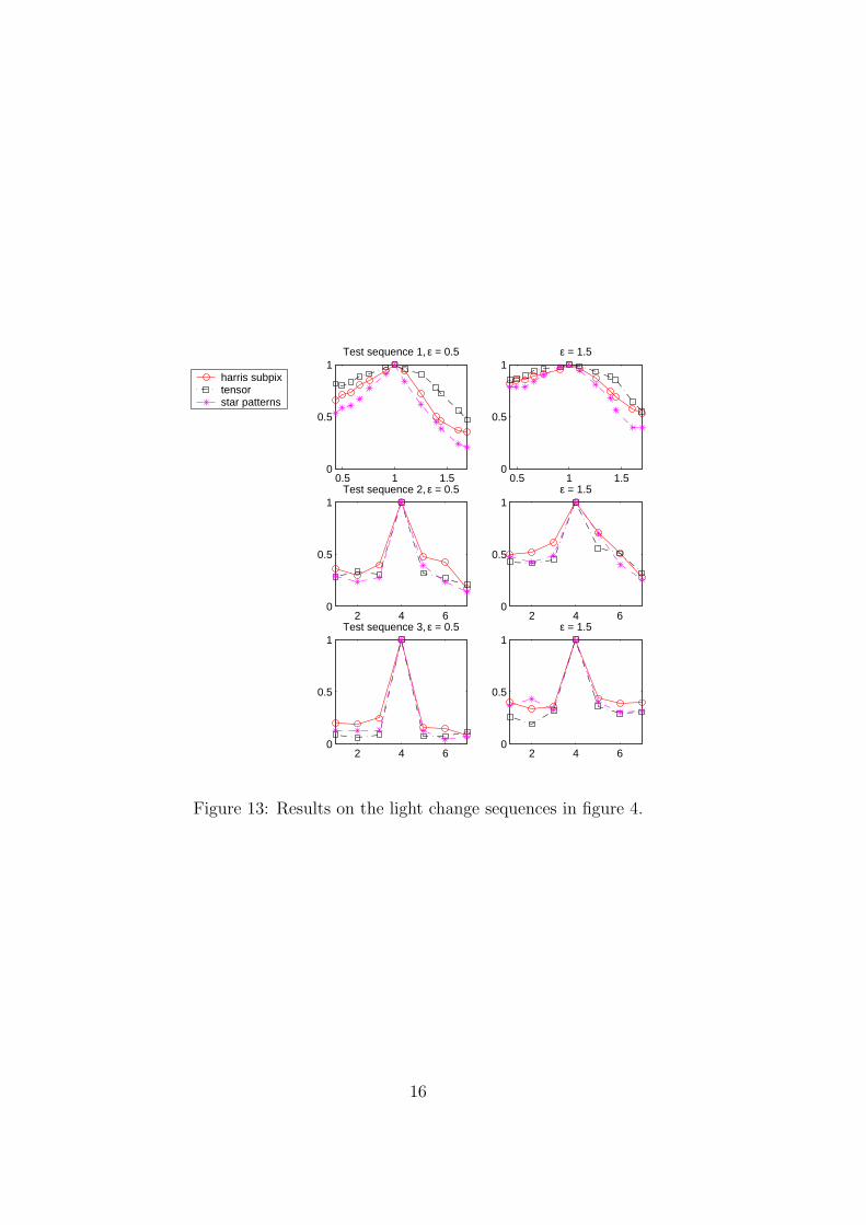
4.3 Variation of illumination
The results on the light transformation sequences is shown in figure 13. We conclude thatthe differences are not significant between the different methods.
5 Conclusions and discussion
From the experiments we may conclude that the choice of operator depends on the im-age content. The star-pattern method and the fourth order tensor assumes a bit moreadvanced model than the Harris operator. These methods has the best performance iftheir corresponding models can describe the image content, as would be expected. If themodel is less valid it seems that it is better to use a more crude model as in the Harrisoperator.
The operators described here is intended to be used in object recognition tasks. Otherinterest point operators have been used in this application, one of the most successfulmethods in recent years is to find local maxima in DoG(Difference of Gaussians) scalespace, see e.g. [6, 7]. These points were also evaluated (using the implementation by
12

1 2 30
0.5
1scale, ε = 0.5
1 2 30
0.5
1ε = 1.5
0 50 100 1500
0.5
1rotation
0 50 100 1500
0.5
1
−40 −20 0 20 400
0.5
1view
−40 −20 0 20 400
0.5
1
harris subpixtensorstar patterns
Figure 7: Result on test image 1 for the rotation, scale, and view transformations.
1 2 30
0.5
1scale, ε = 0.5
1 2 30
0.5
1ε = 1.5
0 50 100 1500
0.5
1rotation
0 50 100 1500
0.5
1
−40 −20 0 20 400
0.5
1view
−40 −20 0 20 400
0.5
1
harris subpixtensorstar patterns
Figure 8: Result on test image 2 for the rotation, scale, and view transformations.
13

1 2 30
0.5
1scale, ε = 0.5
1 2 30
0.5
1ε = 1.5
0 50 100 1500
0.5
1rotation
0 50 100 1500
0.5
1
−40 −20 0 20 400
0.5
1view
−40 −20 0 20 400
0.5
1
harris subpixtensorstar patterns
Figure 9: Result on test image 3 for the rotation, scale, and view transformations.
1 2 30
0.5
1scale, ε = 0.5
1 2 30
0.5
1ε = 1.5
0 50 100 1500
0.5
1rotation
0 50 100 1500
0.5
1
−40 −20 0 20 400
0.5
1view
−40 −20 0 20 400
0.5
1
harris subpixtensorstar patterns
Figure 10: Result on test image 4 for the rotation, scale, and view transformations.
14

1 2 30
0.5
1scale, ε = 0.5
1 2 30
0.5
1ε = 1.5
0 50 100 1500
0.5
1rotation
0 50 100 1500
0.5
1
−40 −20 0 20 400
0.5
1view
−40 −20 0 20 400
0.5
1
harris subpixtensorstar patterns
Figure 11: Result on test image 5 for the rotation, scale, and view transformations.
1 2 30
0.5
1scale, ε = 0.5
1 2 30
0.5
1ε = 1.5
0 50 100 1500
0.5
1rotation
0 50 100 1500
0.5
1
−40 −20 0 20 400
0.5
1view
−40 −20 0 20 400
0.5
1
harris subpixtensorstar patterns
Figure 12: Result on test image 6 for the rotation, scale, and view transformations.
15
0.5 1 1.50
0.5
1Test sequence 1, ε = 0.5
0.5 1 1.50
0.5
1ε = 1.5
2 4 60
0.5
1Test sequence 2, ε = 0.5
2 4 60
0.5
1ε = 1.5
2 4 60
0.5
1Test sequence 3, ε = 0.5
2 4 60
0.5
1ε = 1.5
harris subpixtensorstar patterns
Figure 13: Results on the light change sequences in figure 4.
16
Lowe) on the test images in this report, but the result were poor. However, it is not fairto evaluate the stability for an operator that is computed in several scales. The largerscales may be less stable, but that may not matter if your descriptor is computed in aregion that is proportional to the scale of the interest points.
Acknowledgments
We gratefully acknowledge the support from the Swedish Research Council through agrant for the project A New Structure for Signal Processing and Learning, and the Euro-pean Commission through the VISATEC project IST-2001-34220 [12] .
References
[1] J. Bigun. Pattern recognition in images by symmetries and coordinate transforma-tions. Computer Vision and Image Understanding, 68(3):290–307, 1997.
[2] W. Forstner. A framework for low level feature extraction. In Proceedings of the thirdEuropean Conference on Computer Vision, volume II, pages 383–394, Stockholm,Sweden, May 1994.
[3] Bjorn Johansson. Multiscale curvature detection in computer vision. Lic. ThesisLiU-Tek-Lic-2001:14, Dept. EE, Linkoping University, SE-581 83 Linkoping, Sweden,March 2001. Thesis No. 877, ISBN 91-7219-999-7.
[4] Bjorn Johansson and Anders Moe. Patch-duplets for object recognition and poseestimation. Technical Report LiTH-ISY-R-2553, Dept. EE, Linkoping University,SE-581 83 Linkoping, Sweden, November 2003.
[5] Bjorn Johansson and Anders Moe. Patch-duplets for object recognition and poseestimation. In Ewert Bengtsson and Mats Eriksson, editors, Proceedings SSBA’04Symposium on Image Analysis, pages 78–81, Uppsala, March 2004. SSBA.
[6] David G. Lowe. Object recognition from local scale-invariant features. In Proc.ICCV’99, 1999.
[7] David G. Lowe. Local feature view clustering for 3D object recognition. In Proc.CVPR’01, 2001.
[8] K. Mikolajczyk and C. Schmid. A performance evaluation of local descriptors. InIEEE Conference on Computer Vision and Pattern Recognition, pages 257–263, June2003.
[9] K. Nordberg. A fourth order tensor for representation of orientation and position oforiented segments. Technical Report LiTH-ISY-R-2587, Dept. EE, Linkoping Uni-versity, SE-581 83 Linkoping, Sweden, Februari 2004.
17

[10] Klas Nordberg and Robert Soderberg. Detection and estimation of features for es-timation of position. In Ewert Bengtsson and Mats Eriksson, editors, ProceedingsSSBA’04 Symposium on Image Analysis, pages 74–77, Uppsala, March 2004. SSBA.
[11] C. Schmid, R. Mohr, and C. Bauckhage. Evaluation of interest point detectors. Int.Journal of Computer Vision, 37(2):151–172, 2000.
[12] URL: http://www.visatec.info.
18