A remark on accelerated block coordinate descent for

computing the proximity operators of a sum of convex

functions

Antonin Chambolle∗, and Thomas Pock†

January 6, 2015

Abstract

We analyze alternating descent algorithms for minimizing the sum of a quadratic func-

tion and block separable non-smooth functions. In case the quadratic interactions between

the blocks are pairwise, we show that the schemes can be accelerated, leading to improved

convergence rates with respect to related accelerated parallel proximal descent. As an appli-

cation we obtain very fast algorithms for computing the proximity operator of the 2D and

3D total variation.

1 Introduction

We discuss the acceleration of alternating minimization algorithms, for problems of the form

minx=(xi)ni=1

E(x) :=

n∑i=1

fi(xi) +1

2

∣∣∣ n∑i=1

Aixi

∣∣∣2 (1)

where each xi lives in a Hilbert space Xi, fi are “simple” convex lsc functions whose proximity

operator (I + τ∂fi)−1 can be easily evaluated, and the Ai are bounded linear operators from Xi

to a common Hilbert space X .

In general, we can check that for n ≥ 2, alternating minimizations or descent methods do

converge with rate O(1/k) (where k is the number of iterations, see also [10]), and can hardly

be accelerated. This is bad news, since clearly such a problem can be tackled (in “parallel”)

by classical accelerated algorithms such as proposed in [39, 41, 40, 9, 47], yielding a O(1/k2)

convergence rate for the objective. On the other hand, for n = 2 and A1 = A2 = IX (the

identity), we observe that alternating minimizations are nothing but a particular case of “forward-

backward” descent (this is already observed in [20, Example 10.11]), which can be accelerated

by the above-mentioned methods.

∗CMAP, Ecole Polytechnique, CNRS, 91128 Palaiseau, France.

e-mail: antonin.chambolle@cmap.polytechnique.fr†Institute for Computer Graphics and Vision, Graz University of Technology, 8010 Graz, Austria.

Digital Safety & Security Department, AIT Austrian Institute of Technology GmbH, 1220 Vienna, Austria.

e-mail: pock@icg.tugraz.at

1

Beyond these observations, our contribution is to analyze the descent properties of alternating

minimizations (or implicit/explicit gradient steps as in [4, 48, 11], which might be simpler to

perform), and in particular to show that acceleration is possible for general A1, A2 when n = 2.

We also exhibit a structure which makes acceleration possible even for more than two variables.

In these cases, the improvement with respect to a straight descent on the initial problem is

essentially on the constant in the rate of convergence, since the Lipschitz constants in the partial

descents are always smaller than the global Lipschitz constant of the smooth term |∑iAixi|2.

The fact that first order acceleration seems to work for block coordinate descent is easy to

check experimentally, and in some sense it is up to now a bit disappointing that we provide an

explanation only in very trivial cases.

Problems of the form (1) arise in particular when applying Dykstra’s algorithm [23, 13, 27, 6,

19, 20] to project on an intersection of (simple) convex sets, or more generally when computing

the proximity operator

minz

n∑i=1

gi(z) +1

2|z − z0|2 (2)

of a sum of simple convex functions gi(z) (for Dykstra’s algorithm, the gi’s are the characteristic

functions of convex sets).

Clearly, a dual problem to (2) can be written as (minus)

minx=(xi)i

n∑i=1

(g∗i (xi)−⟨xi, z

0⟩) +

1

2

∣∣∣ n∑i=1

xi

∣∣∣2 (3)

which has exactly form (4) with fi(xi) = g∗i (xi)−⟨xi, z

0⟩, and Ai = IX for all i:

minx=(xi)ni=1

n∑i=1

fi(xi) +1

2

∣∣∣ n∑i=1

xi

∣∣∣2, (4)

Dysktra’s algorithm is precisely an alternating minimization method for solving (4). Then, z is

recovered by letting z = z0 −∑i xi.

Alternating minimization schemes for (1) (and more general problems) are widely found in the

literature, as extensions of the linear Gauss-Seidel method. Many convergence results have been

established, see in particular [4, 28, 45, 6, 19, 20]. Our main results are also valid for linearized

alternating proximal descents, for which [4, 2, 48, 11] have provided convergence results (see

also [3, 14]). In this framework, some recent papers even provide rates of convergence for the

iterates when Kurdyka- Lojasiewicz (KL) inequalities [1] are available, see [48] and, with variable

metrics, the more elaborate results in [18, 25]. In this note, we are rather interested in rates of

convergence for the objective, which do not rely on KL inequalities and a KL exponent but are,

in some cases, less informative.

In this context, two other series of very recent works are closer to our study. He, Yuan and

collaborators [30, 26] have issued a series of papers where they tackle precisely the minimization

of the same kind of energies, as a step in a more global Alternating Directions Method of

Multipliers (ADMM) for energies involving more than two blocks. They could show a O(1/k)

rate of convergence of a measure of optimality for two classes of methods, one which consists into

grouping the blocks into two subsets (which boils down then to the classical ADMM), another

2

which consists in updating the step with a “Gaussian back substitution” after the descent steps.

While some of their inequalities are very similar to ours, it does not seem that they give any new

insight on acceleration strategies for (1).

On the other hand, two papers of Beck and Beck, Tetruashvili [10, 8] address rates of conver-

gence for alternating descent algorithms, showing in a few cases a O(1/k) decrease of the objective

(and O(1/k2) for some smooth problems). It is simple to show, adapting these approaches, that

the same rate holds for the alternating minimization or proximal descent schemes for (1) (which

do not a priori enter the framework of [10, 8]). In addition, we exhibit a few situations where

acceleration is possible, using the relaxation trick introduced in the FISTA algorithm [9] (see

also [29, 39]). Unfortunately, these situations are essentially cases where the variable can be

split into two sets of almost independent variables, limiting the number of interesting cases.

We describe however in our last section that quite interesting examples can be solved with this

technique, leading to a dramatic speed-up with respect to standard approaches.

Eventually, stochastic alternating descents methods have been studied by many authors, in

particular to deal with problems where the full gradient is too complicated to evaluate. First order

methods with acceleration are discussed in [42, 36, 35, 24]. Some of these methods achieve very

good convergence properties, however the proofs in these papers do not shed much light on the

behaviour of deterministic methods, as the averaging typically will get rid of the antisymmetric

terms which create difficulties in the proofs (and, up to now, prevent acceleration for general

problems).

The plan of this paper is as follows: in the next section we recall the standard descent rule

for the forward-backward splitting scheme (see for instance [21]), and show how it yields an

accelerated rate of convergence for the FISTA overrelaxation. We also recall that this is exactly

equivalent to the alternating minimization of problems of form (4) with n = 2 variables.

Then, in the following section, we introduce the linearized alternating proximal descent

scheme for (1) (which is also found in [48, 11], for more general problems). We give a rate

of convergence for this descent, and exhibit cases which can be accelerated.

In the last section we illustrate these schemes with examples of possible splitting for solving

the proximity operator of the Total Variation in 2 or 3 dimensions. This is related to recent

domain decomposition approaches for this problem, see for instance [31].

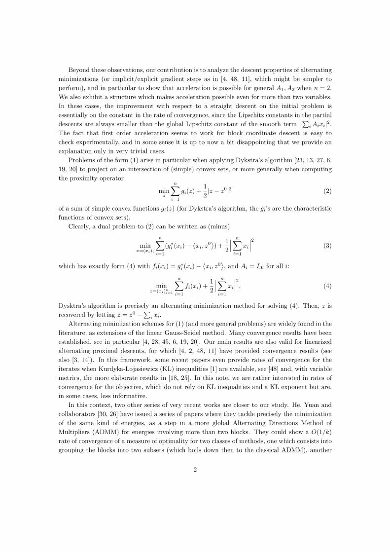
2 The descent rule for Forward-Backward splitting and its

consequences

2.1 The descent rule

Consider the standard problem

minx∈X

f(x) + g(x) (5)

where f is a proper convex lsc function and g is a C1,1 convex function, whose gradient has

Lipschitz constant L, both defined on a Hilbert space X . We can define the simple Forward-

3

Backward descent scheme as the iteration of the operator:

T x = x := (I + τ∂f)−1(I − τ∇g)(x). (6)

Then, it is well-known [40, 9] that the objective F (x) = f(x)+g(x) satisfies the following descent

rule:

F (x) +1

2τ|x− x|2 ≥ F (x) +

1

2τ|x− x|2 (7)

as soon as τ ≤ 1/L. An elementary way to show this is to observe that x is the minimizer of the

strongly convex function f(x) + 〈∇g(x), x〉+ |x− x|2/(2τ), so that

f(x) + g(x) +|x− x|

2τ

2

≥ f(x) + g(x) + 〈∇g(x), x− x〉+|x− x|

2τ

2

≥ f(x) + g(x) + 〈∇g(x), x− x〉+|x− x|

2τ

2

+|x− x|

2τ

2

≥ f(x) + g(x) +

(1

τ− L

)|x− x|

2

2

+|x− x|

2τ

2

where in the last line, we have used the fact that ∇g is L-Lipschitz.

One derives easily that the standard Forward-Backward descent scheme (which consists in

letting xk+1 = Txk) converges with rate O(1/k), and precisely that if x∗ is a minimizer,

F (xk)− F (x∗) ≤ L |x∗ − x0|2

2k(8)

if τ = 1/L.

2.2 Acceleration

However, it is easy to derive from (7) a faster descent, as shown in [9] (see also [39, 40, 41, 47]).

Indeed, letting in (7)

x = xk+1, x = xk +tk − 1

tk+1(xk − xk−1), x =

(tk+1 − 1)xk + x∗

tk+1

(and x−1 := x0) and rearranging, for a given sequence of real numbers tk ≥ 1, we obtain

|(tk+1 − 1)xk + x∗ − tk+1xk+1|

2τ

2

+ t2k+1(F (xk+1)− F (x∗))

≤ |(tk − 1)xk−1 + x∗ − tkxk|2τ

2

+ (t2k+1 − tk+1)(F (xk)− F (x∗))

If t2k+1 − tk+1 ≤ t2k, this can easily iterated. For instance, letting tk = (k + 1)/21 and τ = 1/L,

one finds

F (xk)− F (x∗) ≤ 2L|x∗ − x0|2

(k + 1)2(9)

which is nearly optimal in regards to the lower bounds shown in [38, 40].

What is interesting to observe, here, is that this acceleration property will be true for any

scheme for which a descent rule such as (7) holds, with the same proof. We will now show that

this is also the case for an alternating descent of the form (4), if n = 2.

1Other choices might yield better properties, see in particular [17].

4

2.3 The descent rule for two-variables alternating descent

Consider now problem (4), with n = 2:

minx=(x1,x2)∈X 2

E2(x) := f1(x1) + f2(x2) +1

2|x1 + x2|2. (10)

We consider the following algorithm, which transforms x into T x = x by letting

x1 := arg minx1

f1(x1) +1

2|x1 + x2|2 (11)

x2 := arg minx2

f2(x2) +1

2|x1 + x2|2. (12)

Then by strong convexity, for any x1 ∈ X , we have

f1(x1) +1

2|x1 + x2|2 ≥ f1(x1) +

1

2|x1 + x2|2 +

1

2|x1 − x1|2

while for any x2 ∈ X ,

f2(x2) +1

2|x1 + x2|2 ≥ f2(x2) +

1

2|x1 + x2|2 +

1

2|x2 − x2|2.

Summing these inequalities, we find

f1(x1) + f2(x2) +1

2|x1 + x2|2 ≥

f1(x1) + f2(x2) +1

2|x1 + x2|2 +

1

2|x1 − x1|2 +

1

2|x2 − x2|2

+1

2

(|x1 + x2|2 − |x1 + x2|2 + |x1 + x2|2 − |x1 + x2|2

).

Now, the last line in this equation is

(x1 − x1)(x2 − x2) =1

2|x1 + x2 − (x1 + x2)|2 − 1

2|x1 − x1|2 −

1

2|x2 − x2|2

and it follows

f1(x1) + f2(x2) +1

2|x1 + x2|2 +

1

2|x2 − x2|2

≥ f1(x1) + f2(x2) +1

2|x1 + x2|2 +

1

2|x2 − x2|2. (13)

As before, one easily deduces the following result:

Proposition 1. Let x0 = x−1 be given and for each k let xk2 = xk2 + k−1k+2 (xk2 − xk−1

2 ), xk+11

minimize E2(·, xk2) and xk+12 minimize E2(xk+1

1 , ·). Call x∗ a global minimizer of E2. Then

E2(xk)− E2(x∗) ≤ 2|x∗2 − x0

2|2

(k + 1)2. (14)

5

However, we have to precise here that this result is the same as the main result in [9] recalled

in the previous section, for elementary reasons which we explain in the next Section 2.4. Observe

on the other hand that a straight application of [9] to problem (10) (with |x1 + x2|2/2 as the

smooth term), that is, governed by the iteration(x1

x2

)=

(I + τ

(∂f1

∂f2

))−1(x1 − τ(x1 + x2)

x2 − τ(x1 + x2)

),

needs τ ≤ 1/2 and hence yields the estimate

E2(xk)− E2(x∗) ≤ 4|x∗1 − x0

1|2 + |x∗2 − x02|2

(k + 1)2.

which is less good than (14), whereas the parallel algorithm in [24], with a deterministic block

(x1, x2), is achieving the same rate.

2.4 The two previous problems are identical

In fact, what is not obvious at first glance is that problem (5) and (10) are exactly identical, while

the Forward-Backward descent scheme for the first is the same as the alternating minimization for

the second. A similar remark is already found in [20, Example 10.11]. Indeed, g has L-Lipschitz

gradient if and only if there exists a convex function g0 such that

g(x) = miny∈X

g0(y) + L|x− y|

2

2

. (15)

(An elementary way to show this is to consider that g∗, the Legendre-Fenchel transform of

g, is (1/L)-strongly convex, which means that g∗ − (1/L)|z|2/2 is convex. The function g0 is

then obtained as the Legendre-Fenchel transform of the latter.) It is also standard (see for

instance [15]) that the minimizer y in (15) is nothing else as the point x− (1/L)∇g(x).

Hence, (5) can be rewritten as the minimization problem

minx,y∈X

f(x) + g0(y) + L|x− y|

2

2

. (16)

and the Forward-Backward scheme (6) with step τ = 1/L is an alternating descent scheme for

problem (16), first minimizing in y and then in x.

Observe that the descent rule (13) is a bit more precise, though, than (7). In particular, it

also implies the same accelerated rate for the scheme (minimizing first in x, and then in y):

xk+1 = (I + τ∂f)−1(yk + tk−1

tk+1(yk − yk−1)

)(17)

yk+1 = xk+1 − τ∇g(xk+1) (18)

with tk as before, which coincides with [9] only when ∇g is linear.

6

3 Proximal alternating descent

Now we turn to problem (1) which is a bit more general, and less trivially reduced to another

standard problem as in the previous section. In general, we can not always assume that it is

possible to exactly minimize (1) with respect to one variable xi. However, we can perform a

gradient descent on the variable xi by solving problems of the form

minxi

fi(xi) +

⟨Aixi,

∑j

Aj xj

⟩+〈Mi(xi − xi), xi − xi〉

2τi

for any given x, where Mi is a nonnegative operator defining a metric for the variable xi as soon

as fi is “simple” enough in the given metrics. Then, in case Mi/τi is precisely A∗iAi, the solution

of this problem is a minimizer of

minxi

fi(xi) +1

2

∣∣∣Aixi +∑j 6=i

Aj xj

∣∣∣2,so that the alternating minimization algorithm can be considered as a special case of the alter-

nating descent algorithm (which will require only Mi/τi ≥ A∗iAi). In the sequel to simplify we

will consider the standard metric corresponding to Mi = IXi, however any other metric for which

the prox of fi could be calculated is admissible in practice. Hence we will focus on alternating

descent steps for problem (1) in the standard metrics. The alternating proximal scheme seems

to be first found in [4, Alg. 4.1], while the linearized version we are focusing is proposed and

studied in [48, 11, 18, 25].

This can be described as follows: we let for each i, τi > 0, and we produce x by minimizing

minxi

fi(xi) +

⟨xi, A

∗i

(∑j<i

Aj xj +∑j≥i

Aj xj

)⟩+|xi − xi|

2τi

2

.

Now, for all xi,

fi(xi) +1

2

∣∣∣Aixi +∑j<i

Aj xj +∑j>i

Aj xj

∣∣∣2 +|xi − xi|

2τi

2

=

fi(xi) +1

2

∣∣∣∑j<i

Aj xj +∑j≥i

Aj xj

∣∣∣2 +

⟨xi − xi, A∗i

(∑j<i

Aj xj +∑j≥i

Aj xj

)⟩

+1

2

∣∣∣Ai(xi − xi)∣∣∣2 +|xi − xi|

2τi

2

≥ fi(xi) +1

2

∣∣∣∑j<i

Aj xj +∑j≥i

Aj xj

∣∣∣2 +

⟨xi − xi, A∗i

(∑j<i

Aj xj +∑j≥i

Aj xj

)⟩

+1

2

∣∣∣Ai(xi − xi)∣∣∣2 +|xi − xi|

2τi

2

+|xi − xi|

2τi

2

= fi(xi) +1

2

∣∣∣∑j≤i

Aj xj +∑j>i

Aj xj

∣∣∣2 − 1

2

∣∣∣Ai(xi − xi)∣∣∣2+

1

2

∣∣∣Ai(xi − xi)∣∣∣2 +|xi − xi|

2τi

2

+|xi − xi|

2τi

2

7

Letting for each i, Bi = (1/τi)I −A∗iAi and assuming Bi ≥ 0, it follows

fi(xi) +1

2

∣∣∣Aixi +∑j<i

Aj xj +∑j>i

Aj xj

∣∣∣2 +|xi − xi|2Bi

2≥

fi(xi) +1

2

∣∣∣∑j≤i

Aj xj +∑j>i

Aj xj

∣∣∣2 +|xi − xi|2Bi

2+|xi − xi|

2τi

2

(19)

Summing over all i, we find:

E(x) +‖x− x‖2B

2≥ E(x) +

‖x− x‖2B2

+

n∑i=1

|xi − xi|2τi

2

+1

2

∣∣∣ n∑j=1

Ajxj

∣∣∣2 − ∣∣∣ n∑j=1

Aj xj

∣∣∣2

+

n∑i=1

∣∣∣∑j≤i

Aj xj +∑j>i

Aj xj

∣∣∣2 − ∣∣∣Aixi +∑j<i

Aj xj +∑j>i

Aj xj

∣∣∣2 (20)

where ‖x‖2B =∑ni=1 |xi|2Bi

. Denoting yi = Aixi we can rewrite the last two lines of this formula

(with obvious notation) as follows:

− 1

2

∣∣∣ n∑i=1

yi − yi∣∣∣2 +

n∑i=1

⟨yi − yi,

∑jyj

⟩+

n∑i=1

⟨yi − yi,

∑j<iyj +

yi + yi2

+∑j>iyj

⟩

= −1

2

∣∣∣ n∑i=1

yi − yi∣∣∣2 +

1

2

n∑i=1

|yi − yi|2

+

n∑i=1

⟨yi − yi,

∑j<i(yj − yj) +

∑j>i(yj − yj)

⟩(21)

Notice then that

n∑i=1

⟨yi − yi,

∑j<i(yj − yj)

⟩=

n∑j=1

∑i>j

〈yi − yi, yj − yj〉

=

n∑i=1

∑i<j

〈yj − yj , yi − yi〉 =1

2

n∑i=1

⟨yi − yi,

∑j 6=i(yj − yj)

⟩

=1

2

(∣∣∣ n∑i=1

yi − yi∣∣∣2 − n∑

i=1

|yi − yi|2)

(22)

so that (21) boils down ton∑i=1

⟨yi − yi,

∑j>i(yj − yj)

⟩.

8

One deduces from (20) that for all x,

E(x) +‖x− x‖2B

2≥ E(x) +

‖x− x‖2B2

+

n∑i=1

⟨Ai(xi − xi),

∑j>iAj(xj − xj)

⟩+

n∑i=1

|xi − xi|2τi

2

. (23)

This can also be written

E(x) +‖x− x‖2B

2≥ E(x) +

‖x− x‖2B2

+‖x− x‖2B

2

+1

2

n∑i=1

|Ai(xi − xi)|2 +

n∑i=1

⟨Ai(xi − xi),

∑j>iAj(xj − xj)

⟩. (24)

Then, using (22) again, one has

1

2

n∑i=1

|Ai(xi − xi)|2 +

n∑i=1

⟨Ai(xi − xi),

∑j>iAj(xj − xj)

⟩=

1

2

n∑i=1

|yi − yi|2 +

n∑i=1

⟨yi − yi,

∑j>i(yj − yj)

⟩+

n∑i=1

⟨yi − yi,

∑j>i(yj − yj)

⟩1

2

∣∣∣ n∑i=1

yi − yi∣∣∣2 +

n∑i=1

⟨yi − yi,

∑j>i(yj − yj)

⟩.

which, combined to (24), yields also the following estimate:

E(x) +‖x− x‖2B

2≥ E(x) +

‖x− x‖2B2

+‖x− x‖2B

2

+1

2

∣∣∣ n∑i=1

Ai(xi − xi)∣∣∣2 +

n∑i=1

⟨Ai(xi − xi),

∑j>iAj(xj − xj)

⟩. (25)

3.1 A O(1/k) convergence rate

Convergence of the alternating proximal minimization scheme in this framework (and more gen-

eral ones, see for instance [4]), in the sense that (xk) is a minimizing sequence, is well-known and

not so difficult to establish. In case the energy is coercive, we can obtain from (23) a O(1/k)

decay estimate after k × n alternating minimizations, following essentially the similar proofs

in [10, 8]. The idea is first to consider x = x in (23), yielding

E(x) ≥ E(x) +‖x− x‖2B

2+

n∑i=1

|xi − xi|2τi

2

.

In particular, if x∗ is a solution, letting x = xk, it follows

E(xk+1)− E(x∗) +‖xk+1 − xk‖2B

2+

n∑i=1

|xk+1i − xki |

2τi

2

≤ E(xk)− E(x∗) (26)

9

A rate will follow if we can show that ‖x − x‖ bounds E(x) − E(x∗). From (25) we obtain,

choosing x = x∗,

E(x)− E(x∗) +‖x− x‖2B

2+‖x∗ − x‖2B

2

+1

2

∣∣∣ n∑i=1

Ai(x∗i − xi)

∣∣∣2 +

n∑i=1

⟨Ai(xi − x∗i ),

∑j>iAj(xj − xj)

⟩≤ ‖x

∗ − x‖2B2

Now, since‖x∗ − x‖2B

2− ‖x− x‖

2B

2− ‖x

∗ − x‖2B2

= 〈x− x∗, x− x〉B

this is also

E(x)− E(x∗) +1

2

∣∣∣ n∑i=1

Ai(x∗i − xi)

∣∣∣2 ≤ 〈x− x∗, x− x〉B − n∑i=1

⟨Ai(xi − x∗i ),

∑j>iAj(xj − xj)

⟩,

and there exists C (depending on the Ai’s) such that

E(xk+1)− E(x∗) ≤ C

√√√√ n∑i=1

|xk+1i − xki |

2τi

2

‖xk+1 − x∗‖.

Thus, (26) yields, letting ∆k := E(xk)− E(x∗),

∆k+1 +1

C2‖xk+1 − x∗‖2∆2k+1 ≤ ∆k. (27)

It follows:

Proposition 2. Assume that E is coercive. Then the alternating minimization algorithm pro-

duces a sequence (xk) such that

E(xk)−min E ≤ O(

1

k

).

Proof. Indeed, if E is coercive, one has that ‖xk − x∗‖ is a bounded sequence and (27) reads

∆k+1 + C∆2k+1 ≤ ∆k. (28)

Then, it follows from [8, Lemma 3.6] that

∆k ≤ max

{∆0

2k−12

,4

C(k − 1)

}.

For the reader’s convenience, we give a variant of Amir Beck’s proof, which shows a slightly

different estimate (and that, in fact, asymptotically, the “4” can be reduced). We can let xk =

C∆k, with this normalization we get that

xk+1(1 + xk+1) ≤ xk ⇒ xk+1 ≤−1 +

√1 + 4xk2

,

10

and

xkx−2k+1 − x

−1k+1 − 1 ≥ 0

so that1

xk+1≥ 1 +

√1 + 4xk

2xk≥ 1

xk+ 1− xk. (29)

Notice that from the first relationship, we find that

xk+1 +1

4≤ xk+1 +

1

2≤√xk +

1

4

which yields

xk+1 ≤(x0 +

1

4

) 1

2k+1

− 1

2.

In particular it takes only

k ≥ log log(x0 + 1/2)− log log 5/4

log 2

iterations to reach xk ≤ 3/4, which is for instance 7 iterations if x0 ≈ 1020, and one more iteration

to reach xk+1 ≤ 1/2. Then thanks to (29), one has for k ≥ k + 1 that 1/xk+1 ≥ 1/xk + 1/2 ≥1/xk+1 +(k− k)/2, yielding C∆k ≤ (2+ ε)/k for any ε > 0 and k large enough. Using (29) again

one sees that this bound can, in fact, be made as close as wanted to 1/k (but for k large).

Remark 1. One can observe that as xk converges to the set of solutions (which will be true in

finite dimension), then the constant C ≥ 1/(C2‖xk+1 − x∗‖2) in (28) is improving, yielding a

better actual rate. In particular if E satisfies in addition a Kurdyka- Lojasiewicz type inequality [1]

near a limiting point x∗, then this global rate should be improved (see [48, 18, 25] for rates on

the iterates in this situation).

3.2 The case n = 2

In case n = 2, the situation is simpler (as for the alternating minimizations, for which [10] already

showed that acceleration is possible for smooth functions). Indeed, (23) shows that

E(x) +‖x− x‖2B

2

≥ E(x) +‖x− x‖2B

2+ 〈A1(x1 − x1), A2(x2 − x2)〉+

1

2

n∑i=1

|xi − xi|2τi

2

≥ E(x) +‖x− x‖2B

2− |A1(x1 − x1)|

2

2

− |A2(x2 − x2)|2

2

+1

2

n∑i=1

|xi − xi|2τi

2

so that

E(x) +|x1 − x1|2B1

2+|x2 − x2|

2τ2

2

≥ E(x) +‖x− x‖2B

2+|x1 − x1|2B1

2+|x2 − x2|

2τ2

2

(30)

This makes the FISTA acceleration of [9] possible for this scheme, yielding the rate

E(xk)− E(x∗) ≤ 2

(k + 1)2

(|x0

1 − x∗1|2B1+|x0

2 − x∗2|τ2

)11

as explained in Section 2.2. If one can do an exact minimization with respect to x1, one has in

addition B1 = 0 and falls back into the situation described in Section 2.3. Moreover, if one also

performs exact minimizations with respect to x2, then the rate becomes

E(xk)− E(x∗) ≤ 2|x0

2 − x∗2|A∗2A2

(k + 1)2

which is the generalization of (14).

3.3 A more general case which can be accelerated

In fact, the case n = 2 is a particular case of a more general situation where the interaction term

can be written as the sum of pairwise interactions between two variables xi and xj .

Formally, it means that for all i, j, there exists Ai,j a bounded linear operator from Xi to a

Hilbert space Xi,j = Xj,i such that for all x = (xi)ni=1 ∈ ×ni=1Xi,∣∣∣ n∑

j=1

Ajxj

∣∣∣2 =∑

1≤i<j≤n

|Ai,jxi +Aj,ixj |2.

In this case, one checks that for any (xi, xj) ∈ Xi ×Xj , if i < j then

〈Aixi, Ajxj〉 = 〈Ai,jxi, Aj,ixj〉,

while for i = 1, . . . , n,

|Aixi|2 =∑j 6=i

|Ai,jxi|2.

It follows

n∑i=1

⟨Ai(xi − xi),

∑j>iAj(xj − xj)

⟩=

∑1≤i<j≤n

〈Ai,j(xi − xi), Aj,i(xj − xj)〉

≥ −1

2

∑1≤i<j≤n

(|Ai,j(xi − xi)|2 + |Aj,i(xj − xj)|2

)= −1

2

n∑i=1

∑i<j≤n

|Ai,j(xi − xi)|2 −1

2

n∑i=1

∑1≤j<i

|Ai,j(xi − xi)|2,

where in the last term we have exchanged the indices i and j. On the other hand,

1

2

n∑i=1

|Ai(xi − xi)|2 =1

2

n∑i=1

∑j 6=i

|Ai,j(xi − xi)|2

and it follows that

1

2

n∑i=1

|Ai(xi − xi)|2 +

n∑i=1

⟨Ai(xi − xi),

∑j>iAj(xj − xj)

⟩.

≥ 1

2

n∑i=1

∑1≤j<i

|Ai,j(xi − xi)|2 −1

2

n∑i=1

∑1≤j<i

|Ai,j(xi − xi)|2.

12

We therefore deduce from (24) that

E(x) +‖x− x‖2B

2+

1

2

n∑i=1

∑1≤j<i

|Ai,j(xi − xi)|2.

≥ E(x) +‖x− x‖2B

2+‖x− x‖2B

2+

1

2

n∑i=1

∑1≤j<i

|Ai,j(xi − xi)|2. (31)

It follows, once more, that FISTA-like acceleration is possible for this alternating minimization

strategy, yielding the rate

E(xk)− E(x∗) ≤ 2

(k + 1)2

‖x0 − x∗‖2B2

+1

2

n∑i=1

∑1≤j<i

|Ai,j(x0i − x∗i )|2

.

for any minimizer x∗.

4 Application: various splitting strategies for Total Varia-

tion minimization

In this section, we consider different splitting algorithms for minimizing the Rudin, Osher, Fatemi

(ROF) model for total variation (TV)-based image denoising.

minu

TVp(u) +λ

2‖u− f‖22, (32)

where f ∈ RMN is the (noisy) input image and λ > 0 is a regularization parameter. TVp

corresponds to a discrete `p-norm (p ∈ {1, 2}) based approximation of the total variation. We

will denote by u the unique minimizer of (32). The exact definition of the total variation function

TVp will depend on the certain type of the splitting strategy and hence it will be detailed in the

respective sections.

Let us fix some notation. An image x is defined on a M ×N pixel grid with indices (1, 1) ≤(i, j) ≤ (M,N) which is re-organized into a single column vector u ∈ RMN but for the ease of

notation we will keep the structure of the indices. We will also make use of the function

δC(x) =

{0 if x ∈ C∞ else

which denotes the indicator function for a convex set C.

4.1 Chain-based splitting

In this section, we consider the anisotropic version of (32) (p = 1)

minuP(u) = TV1(u) +

λ

2‖u− f‖2, (33)

13

(a) Original image (600× 800) (b) λ = 10

(c) λ = 5 (d) λ = 1

Figure 1: Test image of size 600 × 800 with intensity values in the range [0, 1] used in our

experiments. We consider experiments with different strength of the regularization parameter to

study the behavior of the algorithm in these cases.

which allows a splitting of the total variation as TV1(u) = TVh(u) + TVv(u), where

TVh(u) =

M,N−1∑i,j=1

|ui,j+1 − ui,j |

computes the total variation along the horizontal edges and

TVv(u) =

M−1,N∑i,j=1

|ui+1,j − ui,j |

computes the total variation along the vertical edges. See Figure 2 for a simple example, where the

blue lines correspond to the total variation along the horizontal edges and the red lines correspond

to the total variation along the vertical edges. This splitting has already been considered before,

14

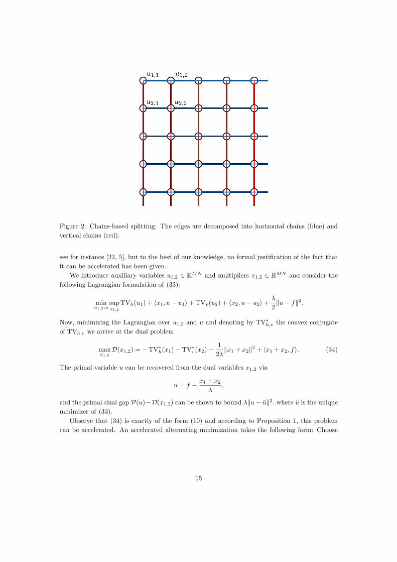
Figure 2: Chains-based splitting: The edges are decomposed into horizontal chains (blue) and

vertical chains (red).

see for instance [22, 5], but to the best of our knowledge, no formal justification of the fact that

it can be accelerated has been given.

We introduce auxiliary variables u1,2 ∈ RMN and multipliers x1,2 ∈ RMN and consider the

following Lagrangian formulation of (33):

minu1,2,u

supx1,2

TVh(u1) + 〈x1, u− u1〉+ TVv(u2) + 〈x2, u− u2〉+λ

2‖u− f‖2.

Now, minimizing the Lagrangian over u1,2 and u and denoting by TV∗h,v the convex conjugate

of TVh,v we arrive at the dual problem

maxx1,2

D(x1,2) = −TV∗h(x1)− TV∗v(x2)− 1

2λ‖x1 + x2‖2 + 〈x1 + x2, f〉. (34)

The primal variable u can be recovered from the dual variables x1,2 via

u = f − x1 + x2

λ,

and the primal-dual gap P(u)−D(x1,2) can be shown to bound λ‖u− u‖2, where u is the unique

minimizer of (33).

Observe that (34) is exactly of the form (10) and according to Proposition 1, this problem

can be accelerated. An accelerated alternating minimization takes the following form: Choose

15

x−12 = x0

2 ∈ RMN , t1 = 1, for each k ≥ 0 compute

tk+1 =1+√

1+4t2k2

xk2 = xk2 + tk−1tk+1

(xk2 − xk−1

2

)xk+1

1 = arg minx1

TV∗h(x1) +1

2‖x1 + xk2 − λf‖2

xk+12 = arg min

x2

TV∗v(x2) +1

2‖xk+1

1 + x2 − λf‖2

. (35)

Thanks to the Moreau identity [7, Thm 14.3], the two last lines of Algorithm (35) can be rewritten

as xk+1

1 = (λf − xk2)− arg minx1

TVh(x1) +1

2‖x1 − (λf − xk2)‖2

xk+12 = (λf − xk+1

1 )− arg minx2

TVv(x2) +1

2‖x2 − (λf − xk+1

1 )‖2.

Both partial minimization problems can be solved by solving M independent one-dimensional

ROF problems on the horizontal chains and N independent one-dimensional ROF problems on

the vertical chains. Efficient direct algorithms to solve one-dimensional ROF problems have been

recently proposed in [22, 34, 5, 32]. The dynamic programming algorithm of [34] seems most

appealing for our purpose since it guarantees a worst case complexity which is linear in the length

of the chain. We will therefore make use of this algorithm.

In the experiments presented in Table 1, we compare the proposed accelerated alternating

minimization (AAM) with respect to a plain alternating minimization (AM) as studied in Sec-

tion 3.1. Similar to the observations made in [43], we observed that the convergence of (35) can

be speeded up by restarting the extrapolation factor (by setting tk = 1) of the algorithm from

time to time. We experimented with different heuristics and best working heuristic turned out

to restart the algorithm whenever the dual energy was increasing within the last 10 iterations.

We denote this variant by (AAM-r).

In Table 2, we test a Open-MP based multi-core implementation of the (AAM-r) algorithm

using a Intel Xeon CPU E5-2690 v2 @ 3.00GHz processor with 20 cores. We stop the (AAM-r)

algorithm as soon as u and x1,2 fulfill

‖u− u‖∞ ≤ ‖u− u‖2 ≤√

(P(u)−D(x1,2))/λ ≤ 1/256,

which ensures that the maximum pixel error of u is less than 1/256 that is the exactly accuracy

of the input data. We compare the performance with a single-core implementation of the graph

cut (GC) based algorithm proposed in [32, 16]2 which utilizes the max-flow algorithm of Boykov

and Kolmogorov [12]. From the timings, one can observe that the proposed algorithm is already

competitive to (GC) using only one core, but a multi-core implementation appears much faster.

We can also observe that (AAM-r) is quite stable with respect to the value of λ.

4.2 Squares based splitting

In this section consider the a discrete approximation of the total variation on squares. Let

s = (s1, s2, s3, s4)T be the nodes of a square, with s1 being the top-left node and enumerating

2The implementation has been taken from http://www.cmap.polytechnique.fr/∼antonin/software/

16

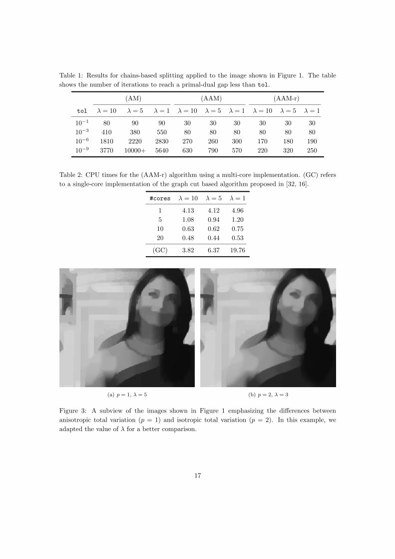
Table 1: Results for chains-based splitting applied to the image shown in Figure 1. The table

shows the number of iterations to reach a primal-dual gap less than tol.

(AM) (AAM) (AAM-r)

tol λ = 10 λ = 5 λ = 1 λ = 10 λ = 5 λ = 1 λ = 10 λ = 5 λ = 1

10−1 80 90 90 30 30 30 30 30 30

10−3 410 380 550 80 80 80 80 80 80

10−6 1810 2220 2830 270 260 300 170 180 190

10−9 3770 10000+ 5640 630 790 570 220 320 250

Table 2: CPU times for the (AAM-r) algorithm using a multi-core implementation. (GC) refers

to a single-core implementation of the graph cut based algorithm proposed in [32, 16].

#cores λ = 10 λ = 5 λ = 1

1 4.13 4.12 4.96

5 1.08 0.94 1.20

10 0.63 0.62 0.75

20 0.48 0.44 0.53

(GC) 3.82 6.37 19.76

(a) p = 1, λ = 5 (b) p = 2, λ = 3

Figure 3: A subview of the images shown in Figure 1 emphasizing the differences between

anisotropic total variation (p = 1) and isotropic total variation (p = 2). In this example, we

adapted the value of λ for a better comparison.

17

Figure 4: Squares-based splitting: The edges are decomposed into small loops (squares) where

red squares have even and blue squares have odd top left indices.

the remaining nodes in clock-wise orientation. On this square we define an operator D ∈ R4×4,

that computes the cyclic finite differences

Ds = (s2 − s1, s3 − s2, s4 − s3, s1 − s4)T , TVp(s) = ‖Ds‖p

and TVp(s) computes the p-norm based total variation on the square s. Figure 3 shows a

qualitative comparison between the anisotropic total variation (p = 1) and the isotropic total

variation (p = 2).

In order to apply the definition of the total variation on squares to the whole image u, we

define a linear operator Si,j that extracts the 4 nodes of the square from the image u with its

top-left node located at (i, j), that is

Si,ju = (ui,j , ui,j+1, ui+1,j+1, ui+1,j)T .

See Figure 4 for a visualization of the splitting. The idea is now to perform a splitting of the

total variation into squares whose top-left nodes have even indices and squares whose top-left

node have odd indices, that is

TVp(u) = TVe(u) + TVo(u),

where TVe(u) corresponds to the total variation on the even squares and TVo(u) corresponds

to the total variation on the odd squares. They are respectively given by

TVe(u) =

bM/2c,bN/2c∑i,j=1

‖DS2i,2ju‖p, TVo =

bM/2c,bN/2c∑i,j=1

‖DS2i−1,2j−1u‖p.

18

Observe that for the ease of notation, we shall skip some edges at the boundaries, which however

can be easily assigned to even or odd squares. In case p = 1 the discretization is equivalent (up to

the skipped edges at the borders) to the discretization on chains. We point out that this splitting

can be extended to higher dimensions using for examples cubes with even and odd origins in 3D.

A similar checkerboard-like decomposition of the total variation has also been adopted in [37] to

perform a block-coordinate descent on the primal ROF model. This algorithm however requires

a smoothing of the total variation in order to guarantee convergence.

Similar to the previous section we derive the dual problem as

maxx1,2

D(x1,2) = −TV∗e(x1)− TV∗o(x2)− 1

2λ‖x1 + x2‖2 + 〈x1 + x2, f〉. (36)

TV∗e,o denote the conjugate functions of TVe,o. A simple computation shows that

TV∗e(x1) =

bM/2c,bN/2c∑i,j=1

δK(S2i,2jx1), TV∗o(x2) =

bM/2c,bN/2c∑i,j=1

δK(S2i−1,2j−1x2),

where K is the convex set defined by

K = {DT ξ : ‖ξ‖q ≤ 1},

where ξ ∈ R4, q =∞ if p = 1 and q = 2 if p = 2.

Observe that the conjugate functions completely decompose into independent problems on

the squares. Hence, it suffices to consider the partial minimization with respect to a single square

of the form

minsδK(s) +

1

2‖s− s‖2, (37)

for some s ∈ R4. Using the definition of K, this problem is equivalent to solving the constraint

quadratic problem

min‖ξ‖q≤1

1

2‖DT ξ − s‖2, (38)

and a minimizer s of (37) can be computed from a minimizer ξ of (38) via s = DT ξ.

4.2.1 The case p = 1

In case p = 1, all constraints on ξ are decoupled. A possibility to solve this problem is to adapt

the graph cut approach [32] which in this case requires only very few computations. However, we

found that it was about twice more efficient to approximately solve this problem by an alternating

minimization scheme. Keeping fixed ξ1,3, we can solve for ξ2,4 via

ξ2 = max

(−1,min

(1,ξ1 + ξ3 + s3 − s2

2

)), ξ4 = max

(−1,min

(1,ξ1 + ξ3 + s1 − s4

2

)).

Likewise keeping fixed ξ2,4, we can globally solve for ξ1,3 using

ξ1 = max

(−1,min

(1,ξ2 + ξ4 + s2 − s1

2

)), ξ3 = max

(−1,min

(1,ξ2 + ξ4 + s4 − s3

2

)).

19

In a practical implementation it turns out that one iteration of this alternating minimization is

enough when storing the values ξ during the iterations and performing a warm start from the

previous solution.

Table 3 compares the proposed accelerated alternating minimization with a standard imple-

mentation of Beck and Teboulle’s algorithm [9] (FISTA) applied to the dual problem (36). We

again tested the accelerated alternating minimization algorithm (AAM) and a variant (AAM-r)

that restarts the overrelaxation parameter whenever the dual energy increased within the last

100 iterations. From the results, on can see that (AAM) needs about 2-3 times less iterations

and (AAM-r) needs about 3-5 times less iterations compared to (FISTA).

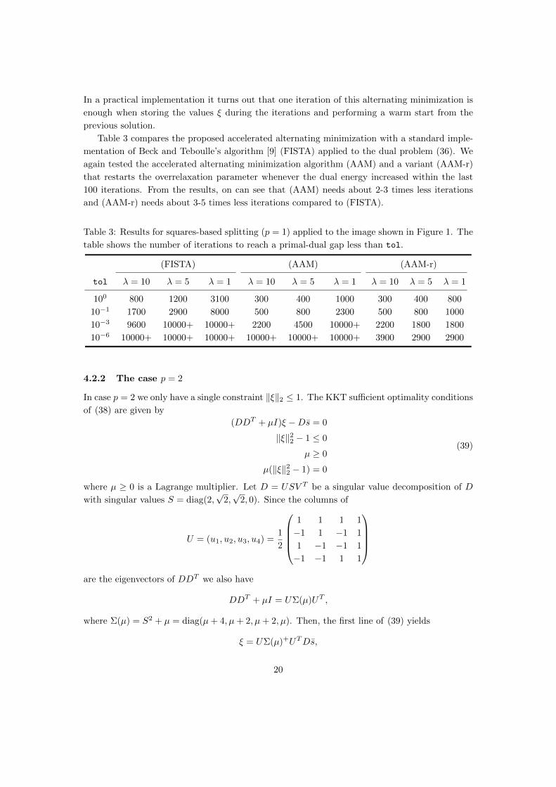
Table 3: Results for squares-based splitting (p = 1) applied to the image shown in Figure 1. The

table shows the number of iterations to reach a primal-dual gap less than tol.

(FISTA) (AAM) (AAM-r)

tol λ = 10 λ = 5 λ = 1 λ = 10 λ = 5 λ = 1 λ = 10 λ = 5 λ = 1

100 800 1200 3100 300 400 1000 300 400 800

10−1 1700 2900 8000 500 800 2300 500 800 1000

10−3 9600 10000+ 10000+ 2200 4500 10000+ 2200 1800 1800

10−6 10000+ 10000+ 10000+ 10000+ 10000+ 10000+ 3900 2900 2900

4.2.2 The case p = 2

In case p = 2 we only have a single constraint ‖ξ‖2 ≤ 1. The KKT sufficient optimality conditions

of (38) are given by

(DDT + µI)ξ −Ds = 0

‖ξ‖22 − 1 ≤ 0

µ ≥ 0

µ(‖ξ‖22 − 1) = 0

(39)

where µ ≥ 0 is a Lagrange multiplier. Let D = USV T be a singular value decomposition of D

with singular values S = diag(2,√

2,√

2, 0). Since the columns of

U = (u1, u2, u3, u4) =1

2

1 1 1 1

−1 1 −1 1

1 −1 −1 1

−1 −1 1 1

are the eigenvectors of DDT we also have

DDT + µI = UΣ(µ)UT ,

where Σ(µ) = S2 + µ = diag(µ+ 4, µ+ 2, µ+ 2, µ). Then, the first line of (39) yields

ξ = UΣ(µ)+UTDs,

20

where Σ(µ)+ denotes the Moore-Penrose-Inverse of Σ(µ), which is well-defined also for µ = 0.

We deduce that

‖ξ‖22 = ‖UΣ(µ)+UTDs‖22 =2(t21 + t22)

(µ+ 2)2+

4t23(µ+ 4)2

,

with t1 =⟨DTu2, s

⟩, t2 =

⟨DTu3, s

⟩, t3 =

⟨DTu1, s

⟩. The optimality system (39) now becomes

2(t21 + t22)

(µ+ 2)2+

4t23(µ+ 4)2

− 1 ≤ 0

µ ≥ 0

µ

(2(t21 + t22)

(µ+ 2)2+

4t23(µ+ 4)2

− 1

)= 0

We solve the reduced system for µ by a projected Newton scheme. We let µ0 ≥ 0 and then, for

each n ≥ 0 we let

µn+1 = max

0, µn −2(t21+t22)(µ+2)2 +

4t23(µ+4)2 − 1

− 4(t21+t22)(µ+2)3 −

8t23(µ+4)3

Once, µ is computed, ξ can be recovered from µ via

ξ = UΣ(µ)+UTDs

It turns out that the above Newton scheme has a very fast convergence. If we perform a warm

start from the previous solution µ during the iterations of the accelerated block descent algorithm,

we observe that 6 Newton iterations are enough to reach an accuracy of 10−20. In practice, the

best overall performance is obtained by doing inexact optimizations using only one Newton

iteration. Additionally, we can perform a simple reprojection of ξ on the constraint ‖ξ‖p ≤ 1

before computing the dual energy to ensure feasibility of the dual problem.

Table 4 presents the results in case of the isotropic (p = 2) total variation on squares. In con-

trast to the setting p = 1, we observed that the restarting strategy did not significantly improve

the convergence and hence we omit the results. In general, the isotropic (p = 2) total variation

appears to be significantly more difficult to optimize compared to the anisotropic (p = 1) total

variation. From the results it can be seen that the proposed accelerated alternating minimization

(AAM) is roughly 3 times faster compared to a standard implementation of (FISTA) applied to

the dual problem (36).

Table 4: Results for squares-based splitting (p = 2) applied to the image shown in Figure 1. The

table shows the number of iterations to reach a primal-dual gap less than tol.

(FISTA) (AAM)

tol λ = 10 λ = 5 λ = 1 λ = 10 λ = 5 λ = 1

100 500 700 1800 200 200 500

10−1 1000 1500 3900 300 500 1200

10−3 5500 8800 10000+ 1500 2400 5900

21

Remark 2. Before closing this subsection, let us observe (cf. Section 3.3) that instead of the red-

black Gauss-Seidel scheme we adopted in the two previous examples, we could also implement

a standard serial Gauss-Seidel scheme, which however did not improve the results and does not

allow for a parallel implementation.

4.3 Disparity estimation

In the last application we consider the problem of computing a disparity image from a pair of

rectified stereo images I l,r. We assume that I l,r are of size M ×N and we consider K ordered

disparity values [d1, ...dk]. We start from the Ishikawa formulation [33, 44] that represents the

non-convex stereo problem as a minimum cut problem in a three-dimensional space.

minui,j,k+1≤ui,j,k

ui,j,k∈{0,1}u·,·,1=1u·,·,K=0

I(u) = TVh(u) + TVv(u) + TVl(u), (40)

where

TVh(u) =∑

1≤i≤M1≤j≤N−1

1≤k≤K

whi,j |ui,j+1,k − ui,j,k|, TVv(u) =∑

1≤i≤M−11≤j≤N1≤k≤K

wvi,j |ui+1,j,k − ui,j,k|,

and

TVl(u) =∑

1≤i≤M1≤j≤N

1≤k≤K−1

ci,j,k|ui,j,k − ui,j,k+1|

The weights wh,vi,j are edge indicator weights that are computed from the left input image I l in

order to yield improved disparity discontinuities. The weights ci,j,k are related to the matching

cost of the left and right image for given disparity values dk at pixel (i, j). The disparity image

di,j is recovered from ui,j,k by letting di,j = dk if ui,j,k − ui,j,k+1 = 1 which can happen only for

one value k ∈ {1, ...,K − 1}.Instead solving (40) using a max-flow algorithm as originally used in [33], we solve a 3D

ROF-like problem:

minvP(v) = I(v) +

1

2‖v − g‖2,

where g is given for all i, j by

gi,j,k =

γ if k = 0

0 if 1 < k < K

−γ if k = K

,

and γ is some positive constant (usually we use γ = 103). It can be shown that if γ is large

enough, the solution v will satisfy for all i, j: vi,j,0 > 0, and vi,j,K < 0. Then, in this case it can

be shown [16] that

ui,j,k =

{0 if vi,j,k ≥ 0

1 if vi,j,k < 0

22

is a solution of (40).

We solve the 3D ROF problem by again performing a splitting into chains. Since this problem

is now 3D, we need to split into three types of chains: horizontal, vertical and in the direction

of the labels. Considering a Lagrangian approach, we arrive at the dual problem

maxx1,2,3

D(x1,2,3) = −TV∗h(x1)− TV∗v(x2)− TV∗l (x3)− 1

2λ‖x1 + x2 + x3‖2 + 〈x1 + x2 + x3, g〉.

Since we now have three blocks, it is not clear that an accelerated alternating minimization

converges (although, in fact, we observed it in practice). We should either perform plain al-

ternating minimization, or we treat two of the variables (e.g. x1,2 = (x1, x2)) as one block on

which we perform a partial proximal descent as investigated in Section 3. It corresponds to a

particular instance of (1) with two blocks (x′1, x′2) given by x′1 = (x1, x2) and x′2 = x3 and with

A1x′1 = x1 + x2 and A2x

′2 = x3. The functions f1, f2 are given by f1(x′1) = TV∗h(x1) + TV∗v(x2)

and f2(x′2) = TV∗l (x3). Furthermore, the step sizes are given by τ ′1 = 1/2 and τ ′2 = 1 which

means that for x′1 we have to perform a descent and for x′2 we can do exact minimization.

The accelerated proximal alternating descent now takes the following form: choose x−11 =

x01 ∈ RMNK , x−1

2 = x02 ∈ RMNK , set τ = 1/2, and set t0 = 1. For each k ≥ 0 compute

tk+1 =1+√

1+4t2k2

xk1,2 = xk1,2 + tk−1tk+1

(xk1,2 − xk−1

1,2

)xk+1

3 = arg minx3

TV∗l (x3) +1

2‖xk1 + xk2 + x3 − λf‖2

xk+11 = arg min

x1

TV∗h(x1) +1

2τ‖x1 − (xk1 − τ(xk1 + xk2 + xk+1

3 − λf))‖2

xk+12 = arg min

x2

TV∗v(x2) +1

2τ‖x2 − (xk2 − τ(xk1 + xk2 + xk+1

3 − λf))‖2.

(41)

Observe that the three proximal steps can be computed as before using an algorithm for mini-

mizing 1D ROF problems.

We present an application to large scale disparity estimation. We use the “Motorcycle” stereo

pair taken from the recently introduced high resolution stereo benchmark data set [46] at half size

(M ×N = 1000×1482). One of the two input images is shown in Figure 5 (a). We discretize the

disparity space in the range of [d1, ..., dk] = [0, ..., 125] pixels. This results in K = 126 discrete

disparity values. The weights ci,j,k are computed using a illumination-robust image matching

cost function. For all i, j, k, we aggregate the truncated absolute differences between the image

gradients of the left and right images in a 2× 2 correlation window:

ci,j,k =1

4

i,j∑m=i−1,n=j−1

min(α, |(I lm+1,n − I lm,n)− (Irm+1,n+dk − Irm,n+dk)|)

+ min(β, |(I lm,n+1 − I lm,n)− (Irm,n+dk+1 − Irm,n+dk)|).

The truncation values are set to α = β = 0.1. The weights wh and wh are computed for all i, j

as follows:

whi,j = λ ·

{µ if |I li,j+1 − I li,j | > δ

1 else, wvi,j = λ ·

{µ if |I li+1,j − I li,j | > δ

1 else,

23

(a) Left image (b) Disparity image

Figure 5: Disparity estimation: (a) shows the left input image of size 1000× 1482 and (b) shows

the disparity image.

Table 5: Results for the 3D ROF model applied to disparity estimation of the image shown in

Figure 5. The table shows the iterations to reach a primal-dual gap less than tol. Note that

due to the size of the problem, a global gap of 100 corresponds to a relative gap (normalized by

the primal energy) of about 6.57 · 10−10.

tol (AM) (AAD)

101 20 20

100 100 50

10−1 390 110

where we set µ = δ = 0.1 and λ = 1/600.

Table 5 shows a comparison of the proposed accelerated alternating descent (AAD) algo-

rithm with a standard alternating minimization (AM) algorithm which has been discussed in

Section 3.1. For both algorithms we again used a multi-core implementation and ran the code

on 20 cores of the same machine, mentioned above. From the table, one can see that (AAD)

is much faster than (AM) especially for computing a higher accurate solution. We point out

that in order to compute the disparity map the 3D ROF model does not need to be solved for

a very high accuracy. Our results suggest that usually 50 iterations are enough to recover the

solution of the minimum cut and hence the optimal disparity image. Note that computing the

2D disparity image amounts for computing a 3D ROF problem of size 1000 × 1482 × 126, that

is solving for 560196000 dual variables! One iteration of the (AAD) algorithm on the 20 core

machine takes about 8.78 seconds, hence the disparity image can be computed in ∼ 250 seconds.

The final disparity image is shown in Figure 5 (b).

24

Acknowledgments

This research is partially supported by the joint ANR/FWF Project Efficient Algorithms for

Nonsmooth Optimization in Imaging (EANOI) FWF No. I1148 / ANR-12-IS01-0003. Thomas

Pock also acknowledges support from the Austrian science fund (FWF) under the START project

BIVISION, Y729. Antonin Chambolle also acknowledges support from the “Programme Gaspard

Monge pour l’Optimisation” (PGMO), through the “MAORI” group.

References

[1] H. Attouch and J. Bolte. On the convergence of the proximal algorithm for nonsmooth

functions involving analytic features. Math. Program., 116(1-2, Ser. B):5–16, 2009.

[2] H. Attouch, J. Bolte, and B. Svaiter. Convergence of descent methods for semi-algebraic and

tame problems: proximal algorithms, forward-backward splitting, and regularized Gauss-

Seidel methods. Math. Program., 137(1-2, Ser. A):91–129, 2013.

[3] H. Attouch, A. Cabot, P. Frankel, and J. Peypouquet. Alternating proximal algorithms

for linearly constrained variational inequalities: application to domain decomposition for

PDE’s. Nonlinear Anal., 74(18):7455–7473, 2011.

[4] A. Auslender. Asymptotic properties of the Fenchel dual functional and applications to

decomposition problems. J. Optim. Theory Appl., 73(3):427–449, 1992.

[5] A. Barbero and S. Sra. Modular proximal optimization for multidimensional total-variation

regularization. Technical report, arXiv:1411.0589, 2014.

[6] H. H. Bauschke and P. L. Combettes. A Dykstra-like algorithm for two monotone operators.

Pac. J. Optim., 4(3):383–391, 2008.

[7] H. H. Bauschke and P. L. Combettes. Convex analysis and monotone operator theory

in Hilbert spaces. CMS Books in Mathematics/Ouvrages de Mathematiques de la SMC.

Springer, New York, 2011. With a foreword by Hedy Attouch.

[8] A. Beck. On the convergence of alternating minimization with applications to iteratively

reweighted least squares and decomposition schemes. Technical Report 4154, Optimization

Online, 2013.

[9] A. Beck and M. Teboulle. A fast iterative shrinkage-thresholding algorithm for linear inverse

problems. SIAM J. Imaging Sci., 2(1):183–202, 2009.

[10] A. Beck and L. Tetruashvili. On the convergence of block coordinate descent type methods.

SIAM J. Optim., 23(4):2037–2060, 2013.

[11] J. Bolte, S. Sabach, and M. Teboulle. Proximal alternating linearized minimization for

nonconvex and nonsmooth problems. Math. Program., 146(1-2, Ser. A):459–494, 2014.

25

[12] Y. Boykov and V. Kolmogorov. An experimental comparison of min-cut/max-flow algo-

rithms for energy minimization in vision. IEEE Trans. Pattern Analysis and Machine In-

telligence, 26(9):1124–1137, September 2004.

[13] J. P. Boyle and R. L. Dykstra. A method for finding projections onto the intersection of

convex sets in Hilbert spaces. In Advances in order restricted statistical inference (Iowa

City, Iowa, 1985), volume 37 of Lecture Notes in Statist., pages 28–47. Springer, Berlin,

1986.

[14] A. Cabot and P. Frankel. Alternating proximal algorithms with asymptotically vanishing

coupling. Application to domain decomposition for PDE’s. Optimization, 61(3):307–325,

2012.

[15] P. Cannarsa and C. Sinestrari. Semiconcave functions, Hamilton-Jacobi equations, and

optimal control. Progress in Nonlinear Differential Equations and their Applications, 58.

Birkhauser Boston, Inc., Boston, MA, 2004.

[16] A. Chambolle and J. Darbon. Image Processing and Analysis with Graphs: Theory and

Practice, chapter A parametric maximul flow approach to discrete total variation minimiza-

tion. CRC Press, 2012.

[17] A. Chambolle and C. Dossal. On the convergence of the iterates of “FISTA”. Preprint

hal-01060130, September 2014.

[18] Emilie Chouzenoux, Jean-Christophe Pesquet, and Audrey Repetti. A block coordinate

variable metric forward-backward algorithm. Preprint hal-00945918, December 2013.

[19] P. L. Combettes. Iterative construction of the resolvent of a sum of maximal monotone

operators. J. Convex Anal., 16(3-4):727–748, 2009.

[20] P. L. Combettes and J.-C. Pesquet. Proximal splitting methods in signal processing.

In Fixed-point algorithms for inverse problems in science and engineering, volume 49 of

Springer Optim. Appl., pages 185–212. Springer, New York, 2011.

[21] P. L. Combettes and V. R. Wajs. Signal recovery by proximal forward-backward splitting.

Multiscale Model. Simul., 4(4):1168–1200, 2005.

[22] L. Condat. A Direct Algorithm for 1-D Total Variation Denoising. IEEE Signal Processing

Letters, 20:1054–1057, November 2013.

[23] R. L. Dykstra. An algorithm for restricted least squares regression. J. Amer. Statist. Assoc.,

78(384):837–842, 1983.

[24] O. Fercoq and P. Richtarik. Accelerated, parallel and proximal coordinate descent. arXiv

preprint arXiv:1312.5799, 2013.

[25] P. Frankel, G. Garrigos, and J. Peypouquet. Splitting methods with variable metric for KL

functions. Preprint hal-00987523, November 2013.

26

[26] X. L. Fu, B. S. He, X. F. Wang, and X. M. Yuan. Block-wise alternating direction method

of multipliers with gaussian back substitution for multiple-block convex programming, 2014.

[27] N. Gaffke and R. Mathar. A cyclic projection algorithm via duality. Metrika, 36(1):29–54,

1989.

[28] L. Grippo and M. Sciandrone. On the convergence of the block nonlinear Gauss-Seidel

method under convex constraints. Oper. Res. Lett., 26(3):127–136, 2000.

[29] Osman Guler. New proximal point algorithms for convex minimization. SIAM J. Optim.,

2(4):649–664, 1992.

[30] B. S. He and X. M. Yuan. Block-wise alternating direction method of multipliers for multiple-

block convex programming and beyond, 2014.

[31] M. Hintermuller and A. Langer. Non-overlapping domain decomposition methods for dual

total variation based image denoising. Journal of Scientific Computing, pages 1–26, 2014.

[32] D. Hochbaum. An efficient algorithm for image segmentation, Markov random fields and

related problems. J. ACM, 48(4):686–701 (electronic), 2001.

[33] H. Ishikawa. Exact optimization for Markov random fields with convex priors. IEEE Trans.

Pattern Analysis and Machine Intelligence, 25(10):1333–1336, 2003.

[34] N. A. Johnson. A dynamic programming algorithm for the fused lasso and L0-segmentation.

J. Comput. Graph. Statist., 22(2):246–260, 2013.

[35] Y. Lee and A. Sidford. Efficient accelerated coordinate descent methods and faster algo-

rithms for solving linear systems. CoRR, abs/1305.1922, 2013.

[36] Q. Lin, Z. Lu, and L. Xiao. An accelerated proximal coordinate gradient method and its

application to regularized empirical risk minimization. Technical Report MSR-TR-2014-94,

Microsoft Research, July 2014.

[37] M. G. McGaffin and J. A. Fessler. Fast edge-preserving image denoising via group coordinate

descent on the GPU. In Proc. SPIE, volume 9020, pages 90200P–90200P–9, 2014.

[38] A. Nemirovski and D. Yudin. Problem complexity and method efficiency in optimization.

A Wiley-Interscience Publication. John Wiley & Sons, Inc., New York, 1983. Translated

from the Russian and with a preface by E. R. Dawson, Wiley-Interscience Series in Discrete

Mathematics.

[39] Yu. Nesterov. A method for solving the convex programming problem with convergence rate

O(1/k2). Dokl. Akad. Nauk SSSR, 269(3):543–547, 1983.

[40] Yu. Nesterov. Introductory lectures on convex optimization, volume 87 of Applied Optimiza-

tion. Kluwer Academic Publishers, Boston, MA, 2004. A basic course.

[41] Yu. Nesterov. Smooth minimization of non-smooth functions. Math. Program., 103(1, Ser.

A):127–152, 2005.

27

[42] Yu. Nesterov. Efficiency of coordinate descent methods on huge-scale optimization problems.

SIAM J. Optim., 22(2):341–362, 2012.

[43] B. O’Donoghue and E. Candes. Adaptive restart for accelerated gradient schemes. Founda-

tions of Computational Mathematics, 2013.

[44] T. Pock, T. Schoenemann, G. Graber, H. Bischof, and D. Cremers. A convex formulation

of continuous multi-label problems. In European Conference on Computer Vision (ECCV),

Marseille, France, October 2008.

[45] M. Razaviyayn, M. Hong, and Z.-Q. Luo. A unified convergence analysis of block successive

minimization methods for nonsmooth optimization. SIAM J. Optim., 23(2):1126–1153, 2013.

[46] D. Scharstein, H. Hirschmuller, Y. Kitajima, G. Krathwohl, N. Nesic, X. Wang, and P. West-

ling. High-resolution stereo datasets with subpixel-accurate ground truth. In German Con-

ference on Pattern Recognition (GCPR 2014), Munster, Germany, September 2014.

[47] P. Tseng. On accelerated proximal gradient methods for convex-concave optimization, 2008.

Submitted to SIAM J. Optim.

[48] Y. Xu and W. Yin. A block coordinate descent method for regularized multiconvex opti-

mization with applications to nonnegative tensor factorization and completion. SIAM J.

Imaging Sci., 6(3):1758–1789, 2013.

28