A Regional Approach to Salience∗

Andrew Ellis† Yusufcan Masatlioglu‡

November 28, 2017

Abstract

We propose a novel regional preference model (RPM) where the framing of thedecision problem affects the salience of a product through the region in which it lies, andthe product’s salience affects the agent’s evaluation. RPM retains the key ingredientsof the salient thinking model of Bordalo et al. [2013b] and allows us to understandthe crux of their approach. RPM also encompasses the loss aversion model of Tverskyand Kahneman [1991] and the status quo bias model of Masatlioglu and Ok [2005],providing a novel connection between three prominent models. We specialize RPM toprovide a behavioral foundation for the salient thinking model to highlight the saliencemodel’s strong predictions and distinguish it from other existing models.

∗We thank David Dillenberger, Erik Eyster, Andrei Schleiffer, Rani Spiegler, Tomasz Strazlecki, CollinRaymond, and conference/seminar participants at BRIC 2017, CETC 2017, SAET 2017, Lisbon Meetings2017, Brown, and Harvard for helpful comments and discussions. This project began at ESSET Gerzensee,whose hospitality is gratefully acknowledged.

†Department of Economics, London School of Economics. Email: a.ellis@lse.ac.uk.‡Department of Economics, University of Maryland. Email: yusufcan@umd.edu

1

1 Introduction

Psychologists have long known that the framing of a decision problem – the context inwhich a decision takes place – plays a significant role in decision making.1 Each frameselects some features of the alternatives to highlight and makes them more salient in theagent’s subsequent evaluation. As described by Taylor and Thompson [1982], this causes“the phenomenon that when one’s attention is differentially directed to one portion on theenvironment rather than to others, the information contained in that portion will receivedisproportionate weighing in subsequent judgments.”

In this paper, we propose and axiomatize a model of salience, which we call the regionalpreference model (RPM). RPM retains the key ingredients of the approach taken by thesalient thinking model of Bordalo et al. [2013b] (henceforth, BGS). Although relatively new,BGS is becoming one of the leading models of individual decision making due to its appealingpsychological motivation and ability to accommodate a variety of disparate evidence.2 Freedfrom the functional form assumptions of BGS, RPM allows us to understand the crux oftheir approach and its implications for choice. Our results reveal a sharp distinction betweenBGS and that of other models sharing similar psychological intuitions, including Gabaix andLaibson [2006], Kőszegi and Szeidl [2013], Bhatia and Golman [2013], Gabaix [2014], Bushonget al. [2015]. RPM also reveals an unexpected connection between BGS and other behavioralmodels that rely on completely different psychological intuitions, as it nests several prominentmodels including Tversky and Kahneman [1991] and Masatlioglu and Ok [2005].

In RPM, the decision maker (henceforth, DM) chooses among alternatives that havedistinct and easily observable attributes in the presence of an exogenously specified frame.3

Each frame divides the product space into different regions according to these attributes.The model’s key feature is that the DM evaluates trade-offs between attributes differentlydepending on the region in which the product lies. Formally, the DM maximizes a weightedsum of the object’s attributes, and in different regions, the weight on each attribute varies.The same product under distinct frames has attributes that are differentially salient and

1See e.g. Tversky and Kahneman [1981], Slovic et al. [1982], Fischer et al. [1986], Rowe and Puto [1987],Frisch [1993], Levin et al. [1998].

2For some recent applications, see Hastings and Shapiro [2013], Busse et al. [2015], Bordalo et al. [2016],Karlan et al. [2016], Gurun et al. [2016], Dertwinkel-Kalt [2016].

3In this paper, the frames are exogenously given. Of course, it is possible that the choice problem itselfhas an influence on determining the frame. We believe that studying endogenous frame formation is animportant and difficult subject, which we leave for future research.

2

may therefore be evaluated differently. In BGS, for example, the attributes are price andquality and the frame is the average price and quality. The regions are determined by whichattribute is further from the frame (average), and this salient dimension receives higherweight than the others.

Despite its generality, RPM makes testable predictions and excludes certain type ofmodeling choices. We provide a complete characterization of the choice behavior equiva-lent to representation by RPM. First, ranking within a region is independent of the frame.Second, preference within a region is well-behaved, in the sense that versions of well-knownaxioms hold within it. Specifically, the preference is monotonic, continuous and linear insidethe region. Overall, RPM enjoys an intuitive and simple axiomatic foundation.

This result highlights an important distinction between model of salience. Of the modelscited above that attempt to capture salience, only BGS is an RPM. In other words, eventhe most general version of BGS excludes these models. Hence BGS offers a completelydifferent method of modeling choice under salience than other existing models. In additionto the salient thinking model of BGS, we show that RPM nests many seemingly unrelatedmodels that have received a great deal of attention in economics. In particular, it includes theconstant loss aversion model of Tversky and Kahneman [1991] (TK) and the linear status quobias model of Masatlioglu and Ok [2005] (MO).4 The loss aversion model is one of the mostinfluential models of behavioral economics. MO is one of the first papers to the study statusquo bias phenomenon by utilizing a choice theoretic approach. As such, RPM can accountfor many phenomena that the traditional rational model cannot, including asymmetric priceelasticities, insensitivity to bad news, endowment effects, and buying-selling price gaps, decoyand compromise effects, and context dependent willingness to pay, among others (Camerer[2004], Bordalo et al. [2012, 2013a,b], Crawford and Meng [2011], Ericson and Fuster [2011]).

BGS, MO and TK have been developed to account for similar decision-making behavior,but they differ substantially in terms of their functional forms. RPM fulfills the challengeof integrating these theories into one cohesive and general model of salience. It allows us tocompare these seemingly unrelated models, and the RPM axioms highlight behavior commonto all three.

We now turn to the model’s distinct predictions for choice. To this end, we provide a4In this paper, for comparison purposes, we consider a straight-forward extension of their model in which

the reference point might be unavailable.

3

complete behavioral characterization of BGS. While TK and MO both provide axiomatiza-tions of their models, the characterization of BGS was an open question. BGS strengthensRPM in two important ways. First, it imposes a particular structure on the regions. Wecharacterize this structure and show that the regions generated by any parametrization areidentical, reference point by reference point. Second, it imposes a particular structure on theutility functions. The most general property is a consistency one: the reference point onlyaffects preference through the regions it generates. The properties more specific to BGS arethat preference reflects across the 45-degree line, and that attribute i gets more weight whenthe product is in the i-salient region.

Our results highlight trade-offs between the different modeling approaches. For instance,BGS maintains a stronger consistency condition across frames than does TK, but TK, unlikeBGS, satisfies monotonicity across regions (in addition to within regions). The strong con-sistency property is normatively appealing – as long as neither alternatives’ salience changes,their relative ranking does not change – and ideally we would like a model that satisfies both.However, the trade-off between the two is a general property of reference-dependent regionalpreferences. Any reference-dependent regional preference that exhibits salient thinking andsatisfies the strong consistency condition either violates monotonicity or has a very particularand hard to interpret structure. This finding does not favor one model over the other, butmake their differences clear. If the strong consistency is desired in an application, then BGScould be a better fit to the job than TK. If monotonicity is a necessary property, TK wouldbe ahead of BGS.

Interpreting regional preferences as arising from differential attention to attributes, RPMhas a close relationship with the literature studying how limited attention affects decisionmaking. Masatlioglu et al. [2012] and Manzini and Mariotti [2014] study a DM who haslimited attention to the alternatives available. The DM maximizes a fixed preference relationover the consideration set, a subset of the alternatives actually available. In contrast, in RPMthe DM the considers all available alternatives but maximizes a preference relation distortedby her attention. Caplin and Dean [2015], de Olivera et al. [2016] and Ellis [2018] studya DM who has limited attention to information. In contrast to RPM, attention is chosenrationally to maximize ex ante utility, rather determined by the framing of the decision, andchoice varies across states of the world. The most related interpretation considers attributesas payoffs in a fixed state. In addition to choices varying across states, each alternative hasthe same weights on each attribute, similar to Kőszegi and Szeidl [2013].

4

2 Model

In this paper, each product has several attributes. For simplicity, we focus on two-attributescase. We let X denote the set of alternatives, and assume that X = I1 ×I2 for open intervalsI1 and I2.5 For x, y ∈ X and α ∈ [0, 1], denote by xαy the coordinate-by-coordinate mixtureof x and y, i.e. [xαy]i = αxi + (1 − α)yi for all i.

We denote the set of frames by F . The frame does not affect the material outcomeof alternatives but may affect their salience. Examples of frames include the reference ordefault option of the consumer, the intensity of advertising, and a lottery over referencebundles (as in Köszegi and Rabin [2006]). In the first example, we set F = X, in the second,we set F = [0, 1], and in the final one, we set F = ∆X. In general, F can be any non-empty,connected subset of a metric space.

For each frame f ∈ F , the DM maximizes a complete and transitive preference relation,denoted by %f . As usual, �f denotes strict preference and ∼f indifference. Our observabledata is thus a family of such preferences indexed by the set of frames, {%f}f∈F .

The first idea of our model is that, given a frame f , the product space is divided intodifferent regions according their salience. Each region corresponds to a different saliency andchanges as the frame changes. We allow the regions to have a very general structure.

Definition 1. A vector-valued function R = (R1, R2, . . . , Rn) is a regional function if eachRi : F → 2X satisfies the following properties:

1. Ri(f) is a non-empty, connected, open set,

2. ⋃ni=1 Ri(f) is dense,

3. Ri(f) ⋂Rj(f) = ∅ for all i 6= j, and

4. Ri(·) is continuous.6

We interpret the properties as follows. Every region contains some bundle for everyframe. If x belongs to the region, then so do all y that are close enough to x. There is a

5For the purposes of our representation theorem, X can be any open, bounded, convex subset of Rn

without changing the arguments.6That is, each Ri is both upper and lower semicontinuous when viewed as a correspondence.

5

path that stays within the region between any two points, so regions cannot be the unionof “islands.” Almost every alternative is in at least one region, and none are in two regions.Finally, if the frame does not change too much, then neither do the regions.

In our model, a consumer values each good with an affine utility function. Utilitydepends not only on consumption of a product, as in the standard neoclassical model, butalso on the region to which the product belongs. Suppose the consumption x lies in the regioni when the frame f , that is, x ∈ Ri(f). Then, the value of consumption x is represented byui(x|f). We require that the frame does not affect the utility trade-off within a region. Inother words, changing frame does not alter the relative ranking of two alternatives as longas both of the alternatives lie in the same region. To capture this feature, we assume thatui(·|f) is a positive and affine transformation of ui(·|f ′). We formally define the regionalpreference model for a regional function R as follows.

Definition 2. The family {%f}f∈F conforms to the regional preference model (RPM) undera given R if there exist n families {ui(·|f)}f∈F of strictly increasing, affine functions, whereui(·|f) is a positive affine transformation of ui(·|f ′) for every f, f ′ ∈ F , such that for allx ∈ Ri(f) and y ∈ Rj(f),

x %f y if and only if ui(x|f) ≥ uj(y|f).

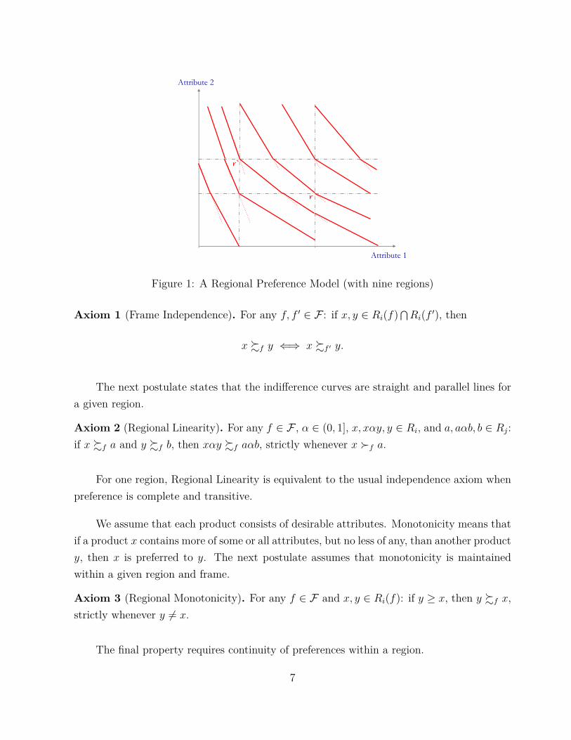
Figure 1 provides an illustration for RPM (à la Köszegi and Rabin [2006]) for a fixedframe f . The frame is a lottery of two deterministic reference points r and r′ with equalprobability. In this example, there are nine different regions.

3 A Behavioral Foundation

In this section, we provide a set of behavioral postulates characterizing RPM. This behaviorrepresents the key features of the model. Theorem 1 shows they hold if and only if the DMis representable by RPM, rendering the model behaviorally testable.

The first postulates states that changing the frame does not alter the relative rankingof two alternatives as long as both of the alternatives lie in the same region.

6

r

r`

Attribute 2

Attribute 1

Figure 1: A Regional Preference Model (with nine regions)

Axiom 1 (Frame Independence). For any f, f ′ ∈ F : if x, y ∈ Ri(f) ⋂Ri(f ′), then

x %f y ⇐⇒ x %f ′ y.

The next postulate states that the indifference curves are straight and parallel lines fora given region.

Axiom 2 (Regional Linearity). For any f ∈ F , α ∈ (0, 1], x, xαy, y ∈ Ri, and a, aαb, b ∈ Rj:if x %f a and y %f b, then xαy %f aαb, strictly whenever x �f a.

For one region, Regional Linearity is equivalent to the usual independence axiom whenpreference is complete and transitive.

We assume that each product consists of desirable attributes. Monotonicity means thatif a product x contains more of some or all attributes, but no less of any, than another producty, then x is preferred to y. The next postulate assumes that monotonicity is maintainedwithin a given region and frame.

Axiom 3 (Regional Monotonicity). For any f ∈ F and x, y ∈ Ri(f): if y ≥ x, then y %f x,strictly whenever y 6= x.

The final property requires continuity of preferences within a region.

7

Axiom 4 (Regional Continuity). For any x ∈ X and f ∈ F : the sets {y ∈ Ri(f) : y �f x}and {y ∈ Ri(f) : x �f y} are open for every i = 1, . . . , n.

Our main result states that these four postulates characterize RPM.

Theorem 1. If R is a regional function, then ({%f}f∈F , R) satisfies Frame Independence,Regional Linearity, Regional Monotonicity and Regional Continuity if and only if {%f}f∈F

conforms to RPM under R.

Theorem 1 highlights the fact that RPM has strong predictive power by providing acomplete characterization. That is, Axioms 1-4 are both necessary and sufficient for themodel, so Theorem 1 lays out all possible implications of regional preferences. This is crucialsince some of these implications are hard to see by looking at the description of the model.This emphasizes the important role of Theorem 1 in understanding of regional preferences.The result provides a set of unifying behavior that underlies and unifies special cases ofRPM, like TK and BGS. Finally, Theorem 1 makes it possible to show that there are othermodels that attempt to capture salience but that are not outside of our framework. Theseinclude the models of Gabaix and Laibson [2006], Kőszegi and Szeidl [2013], Bhatia andGolman [2013], Gabaix [2014], Bushong et al. [2015].7 The common feature of these modelsis that, for a given frame, there is a unique utility function applying to all the alternatives.This feature implies that these models are one-region models. Frame Independence requiresthat the same utility function should be utilized for any other frame since there is only oneregion. Hence, the only model having this feature is the classical model in our framework.

The closest results of which we are aware are found in Segal [1992] and Chapter 2.4of Schmidt [1998].8 Both are concerned with the existence of an additively separable oraffine utility functions on subsets of product spaces or lotteries, such as our regions. Theformer provides conditions for existence of an additively separable utility function on subsetsof product spaces, including that the indifference sets are connected. The latter studiespiecewise affine utility representations over lotteries, where each piece is σ-convex. Noneof their results apply in this setting because their assumptions rule out regions of the formassumed by BGS. Our stronger independence axiom allows us to overcome this limitation.Additionally, neither considers how preferences change with frames.

7See appendix for the functional forms and discussion.8We thank David Dillenberger for bringing the latter to our attention.

8

3.1 Revealing Regions

For our representation result, we took the regions as given. While this assumption simplifiesexposition and statement of the axioms, it places significant demands on the data observed.Nevertheless, if we make stronger assumptions about the slope of the indifference curves, wecan identify the regions directly from the DM’s choices. This subsection discusses how wedo so.

We first identify a potential region around x by an open set where the DM’s choicesreveal straight and parallel indifference curves.

Definition 3. An open set A is a revealed region around x for frame f if x ∈ A, whena, b, aαc, bαc ∈ A we have a %f b ⇐⇒ aαc %f bαc.

That is, a revealed region is an open set for which the preference satisfies our linearityaxiom, or equivalently has linear indifference curves. When the underlying preference con-forms to RPM where each region’s indifference curves have distinct slopes, we can identifythe entire region to which each point belongs. Specifically, the largest revealed region aroundx, in the sense of set inclusion, corresponds to the region specified by the region function.

Proposition 1 (Revealing Regions). Suppose {%f}f∈F conforms to RPM for some regionalfunction R where ui(·|f) is not an affine transformation of uj(·|f) when i 6= j. Then for anyx ∈ X and f ∈ F , there exists a unique maximal region around x for f that equals Ri(f)when x ∈ Ri(f) and equals ∅ when x belongs to no region.

The proposition allows us to identify the regions directly from the preference relation.In particular, it provides a test for whether a given set belongs to the same region as x.Either the set is a subset of the same region as x, or we can find a violation of linearitywithin the set. As an application, the result allows one to check whether the properties ofregions shown by Proposition 1 to hold for BGS are satisfied by looking only at the frameand the agent’s behavior.

3.2 Reference point as frame

In the rest of the paper, we focus primarily on a special case of the model that includes BGS,MO and TK: reference-dependent frames. In this subsection, we formally define regions so

9

that the salience of a good is determined solely by its position relative to a “reference good.”This reference good is the only feature that alters the salience of goods.9 This special caseis of interest in its own right since it covers several well-known models.

We first adjust our definition of R to focus specifically on cases where the referencepoint is the frame. Here, the reference good is the focal point that splits the alternativesaround it. While it does not belong to any particular region, the comparison between thebundles and the reference create the regions. Hence, all regions surround the reference point.To that end, formally, we consider the following modification of a regional function.

Definition 4. The function R = (R1, R2, . . . , Rn) is a reference-dependent regional functionif F = X and each Ri : F → 2X satisfies properties 2, 3 and 4 of Definition 1 and:10

1. Ri(r) is a non-empty open set such that Ri(r) ⋃{r} is connected, and

2. r ∈ ⋂ni=1 bd(Ri(r)).

It is easy to see that RPM with a reference dependent regional function (henceforth,RD-RPM) is a special case of RPM with a standard regional function. We do so by treatingas equivalent any regions with the same utility, provided they are close to the referencepoint.11 This requires that regions look like slices of a pie centered around the referencepoint, and each region may be more than one slice. This rules out, for instance, regions ala Köszegi and Rabin [2006] that do not meet at a single point (see Figure 1). Moreover, itrequires that the regions change with the reference point.

4 Foundations for BGS

BGS propose an intuitive and descriptive behavioral model based on salience, but theyfocus on understanding interesting applications rather than connecting the components of

9We do not specify the reference good, which could be (i) the default option (Tversky and Kahneman[1991], Johnson and Goldstein [2003], Samuelson and Zeckhauser [1988]), (ii) status quo (Tversky and Kah-neman [1991], Johnson and Goldstein [2003], Samuelson and Zeckhauser [1988]), (iii) the average level of eachattribute in the choice set (Kivetz et al. [2004], Bordalo et al. [2013b]), (iv) aspirations/expectations/goals(Payne et al. [1980]) or (v) actual choice (Köszegi and Rabin [2006]).

10To make the distinction we use r instead of f for the reference-dependent regional function.11That is we replace R1(r), ..., Rn(r) with R′

1(r), ..., R′m(r) where, e.g., R′

1(r) =⋃

i Ri(r) where i rangesover {i : ui(·|f) = u1(·|f) for all f ∈ F}.

10

their model to observed choice behavior. It is still an open question what are the full setof behavioral postulates characterizing BGS’ original formulation. This section focuses onclosing that question.

4.1 The BGS Model

In the BGS model, the salience of an attribute depends on the value of the product’s attributeand the reference level of that attribute.12 The amount of salience is determined by a saliencefunction σ, and the attribute with the largest salience is called the salient attribute for thatgood. In general, the different attributes are salient for different goods. The salience functiondoes not depend on either the identity of the products or the particular attribute considered.Each salience function creates two regions: one where attribute 1 is salient and the otherattribute where 2 is salient.

More formally, let (r1, r2) be the reference level. Then attribute 1 is salient for goodx if σ(x1, r1) > σ(x2, r2), and attribute 2 is salient for good x if σ(x1, r1) < σ(x2, r2).BGS assume that σ is continuous and symmetric, i.e. σ(a, b) = σ(b, a). They require twoadditional properties: Ordering and Homogeneity of Degree Zero. Homogeneity of DegreeZero imposes that for all α > 0, σ(αa, αb) = σ(a, b). Ordering states that salience increasesin contrast. Formally, when ε, ε′ ≥ 0 with ε + ε′ > 0, if a > b, then σ(a + ε, b − ε′) > σ(a, b),and if a < b, then σ(a − ε, b + ε′) > σ(a, b). We say that σ is a salience function if it iscontinuous, symmetric and satisfies Ordering and Homogeneity of Degree Zero. In Section4.2, we analyze the regions generated by salience functions. Proposition 2 axiomaticallycharacterizes the regions and shows that, surprisingly, any two salience functions generatethe same regions.

BGS theorize how salience distorts the valuation of a good. For each product, the DMranks puts higher weight on the salient attribute. In other words, if attribute i is salientfor product x, then attribute i attracts more attention than attribute j and receives greaterdecision weight for the valuation of x. In particular, they are represented by the function

VBGS(x|r) =

wx1 + (1 − w)x2 if σ(x1, r1) > σ(x2, r2)(1 − w)x1 + wx2 if σ(x2, r2) > σ(x1, r1)

(1)

12In the original paper, BGS illustrate their model in an environment where one attribute desirable (qual-ity) and the other is undesirable (price). We provide an graphical illustration for such cases in the Appendix.

11

where w ∈ (0.5, 1) increases in the severity of salient thinking.13 The left panel in Figure2 shows BGS regions and the resulting indifference curves for a fixed reference point. InSection 4.3, we provide axioms equivalent to representation by VBGS.

4.2 A Characterization of the BGS Regions

We first ask when a reference-dependent regional function can be derived from a saliencefunction. To study BGS, we assume X = (0, x) × (0, x), where x > 0 throughout thissection.14 Since there are two attributes, there are two regions. Fix a reference-dependentregional function R = (R1, R2). We interpret Ri(r) as the goods that are i-salient for thereference point r. We now state properties which are defined for a reference-dependentregional function. Then we show these properties characterize the BGS’s salience function.

S1 (Moderation) For any λ ∈ (0, 1] and r ∈ X:if x ∈ R−i(r) and yi = λxi + (1 − λ)ri and y−i = x−i, then y ∈ R−i(r).

S2 (Equal Salience) For any x, r ∈ X: if x1r1

= x2r2

or x1r1

= r2x2

, then x /∈ Ri(r) for i = 1, 2.

S3 (Regular regions) For all r ∈ X and i = 1, 2: Ri(r) is a regular open set.15

The properties have natural interpretations. First, making the attribute of a bundlecloser to the reference point’s attribute decreases the salience of that attribute. That is,when x and y differ only in attribute j, and y is closer to the reference in that attribute, if x

is i-salient, then so is y. Second, if every attribute of x differs from the reference point by thesame percentage, then none of the attributes stands out. More formally, if the percentagedifference between xi and ri is the same across attributes, then x is not i-salient for any i.Finally, regions are regular open sets. That is, there is no bundle completely surrounded byi-salient bundles that is not an i-salient bundle itself. Any bundle that can be approached bya sequence of i-salient bundles is either i-salient or on the boundary of the i-salient region.

13BGS parametrize by δ ∈ (0, 1], so their utility function is 2VBGS(x|r) for w = 11+δ .

14BGS focus on the case where one attribute, price, is a “bad.” We can accommodate this by insteadtaking X = (−x, 0) × (0, x) and letting attribute 1 represent the bad. This version of model is illustrated inthe Appendix. To do so, we must replace x1 with −x1 in S1-S3 and alter Axiom 7 as discussed in Footnote16.

15Recall that a set A is regular open if A = int(cl(A)).

12

Proposition 2. The following are equivalent:

(i) The reference-dependent regional function (R1, R2) satisfies S1-S3,

(ii) There exists a salience function σ s.t. x ∈ Ri(r) ⇐⇒ σ(xi, ri) > σ(x−i, r−i),

(iii) For any salience function σ, x ∈ Ri(r) ⇐⇒ σ(xi, ri) > σ(x−i, r−i).

This proposition provides a characterization for BGS’s salience function. In other words,Proposition 2 translates the functional form assumptions on the salience function in termsproperties on the regions. An immediate implication is that any specification of the saliencefunction leads to the same regions.

4.3 A Characterization for BGS

We now identify the additional assumptions to pin down the exact formulation of BGS.These assumptions identify the additional structure imposed by BGS in addition to Axioms1-4. Each corresponds to a particular feature imposed by BGS.

The first property guarantees that the salient attribute gets a higher weight in the utility.

Axiom 5 (Salient Dimension Overweighted; SDO). For any x, y, r, r′ ∈ X:if y ∈ Ri(r) ⋂

Ri(r′), x ∈ Ri(r) ⋂R−i(r′), x %r y and xi > xj, then x �r′ y

SDO requires that regions correspond to the dimension that gets the most weight. Thatis, the DM overvalues a bundle whose best attribute is i more when it is in region i. To seewhy, suppose dimension 1 is the best for bundle x. SDO requires that when x is at least asgood as y when dimension 2 stands out for both, the DM chooses x over y for sure when 1stands out for it.

Second, changing reference point does not reverse the ranking of two products unless italso changes their salience.

Axiom 6 (Strong Frame Independence; SFI). For any x, y, r, r′ ∈ X:If x ∈ Ri(r) ⋂

Ri(r′) and y ∈ Rj(r) ⋂Rj(r′), then x %r y if and only if x %r′ y.

13

For the general RPM, the reference point influences choice trough two channels: salienceand valuation. The axiom eliminates the latter. When comparing two alternatives acrossdifferent reference points, the DM’s relative ranking does not change when neither’s saliencechanges. This property greatly limits the effect of the reference point. In fact, a suffi-ciently small change in the reference never leads to a preference reversal. Notice that FrameIndependence is the special case of SFI where i = j.

Finally, because both salience and preference are symmetric across attributes, permutingthe attributes of all objects in the same way does not change rankings. Thus, our lastadditional axiom requires that the preference “reflects” about the 45 degree line.

Axiom 7 (Reflection). For any x, y, r, r′ ∈ X:(x1, x2) %(r1,r2) (y1, y2) if and only if (x2, x1) %(r2,r1) (y2, y1).

Note that both the reference point and the values of each attribute reverse.16 Relax-ing the symmetry across attributes in terms of either preference or salience would breakreflection. Hence, the behavioral implications of the symmetry assumption is exactly thereflection property.

Theorem 2. Let {%r}r∈X conform to RD-RPM under R = (R1, R2). Then, R satisfiesS1-S3 and ({%r}r∈X , R) satisfies Salient Dimension Overweighted, Strong Frame Indepen-dence, and Reflection if and only if {%r}r∈X has a BGS representation.

Theorem 2 highlights the fact that the salience model of BGS has strong predictionsand can be distinguished from other existing models. In addition, Theorem 2 provides abehavioral foundation for the salience model. Hence it is possible to test the BGS modelnon-parametrically by using a revealed-preference technique. The contrast between the hy-potheses of Theorem 1 and Theorem 2 reveals the additional structure imposed by the BGSmodel. The key properties of BGS are Strong Frame Independence and SDO. One can re-lax its other properties, i.e. reflection and S1-S3, to increase explanatory power withoutsacrificing the main idea of the model.

16If attribute 1 takes only negative values, as discussed above, then the axiom becomes:“For any x, r, y ∈ X, (x1, x2) %(r1,r2) (y1, y2) if and only if (−y2, −y1) %(−r2,−r1) (−x2, −x1).”The intuition is similar, but we must take into account that we are replacing a bad with a good and keep inmind our domain restriction.

14

5 Comparing Models

We have establish that RPM nests the salient thinking model of Bordalo et al. [2013b]. Inthis section, we also show that RPM also covers the constant loss aversion model of Tverskyand Kahneman [1991] and the linear status quo bias model of Masatlioglu and Ok [2005].Our general framework makes it possible to compare these seemingly unrelated models. Wehighlight some of the behaviors in common between these models and allows us to distinguishtheir distinct predictions for choice.

5.1 Models

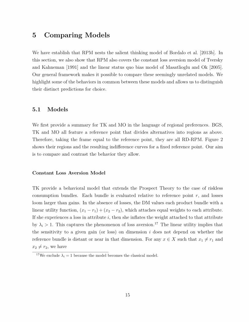
We first provide a summary for TK and MO in the language of regional preferences. BGS,TK and MO all feature a reference point that divides alternatives into regions as above.Therefore, taking the frame equal to the reference point, they are all RD-RPM. Figure 2shows their regions and the resulting indifference curves for a fixed reference point. Our aimis to compare and contrast the behavior they allow.

Constant Loss Aversion Model

TK provide a behavioral model that extends the Prospect Theory to the case of risklessconsumption bundles. Each bundle is evaluated relative to reference point r, and lossesloom larger than gains. In the absence of losses, the DM values each product bundle with alinear utility function, (x1 − r1) + (x2 − r2), which attaches equal weights to each attribute.If she experiences a loss in attribute i, then she inflates the weight attached to that attributeby λi > 1. This captures the phenomenon of loss aversion.17 The linear utility implies thatthe sensitivity to a given gain (or loss) on dimension i does not depend on whether thereference bundle is distant or near in that dimension. For any x ∈ X such that x1 6= r1 andx2 6= r2, we have

17We exclude λi = 1 because the model becomes the classical model.

15

VT K(x|r) =

(x1 − r1) + (x2 − r2) if x1 > r1 and x2 > r2

λ1(x1 − r1) + (x2 − r2) if x1 < r1 and x2 > r2

(x1 − r1) + λ2(x2 − r2) if x1 > r1 and x2 < r2

λ1(x1 − r1) + λ2(x2 − r2) if x1 < r1 and x2 < r2

Notice that there are four different regions in the TK formulation: (i) gain in bothdimensions, (ii) gain in the first dimension and loss in the second dimension, (iii) loss inthe first dimension and gain in the second dimension, and (iv) loss in both dimensions (seeFigure 2). We model this as R = (RGG, RGL, RLG, RLL) where RGG(r) = {x : x � r},RLL(r) = {x : x � r}, RGL(r) = {x : x1 > r1 and x2 < r2} and RLG(r) = {x : x1 <

r1 and x2 > r2}.

Linear Status Quo Bias Model

In the MO model, individuals may experience some form of psychological discomfort whenthey have to abandon their status quo option. This discomfort imposes an additional utilitycost. Of course, if an alternative is unambiguously superior to the status quo, the DM doesnot feel any psychological discomfort to forgo the status quo; in such cases there will beno cost. Formally, Q(r) is a closed set denoting the alternatives that are unambiguouslysuperior to the default option r (see Figure 2). If an alternative does not belong to this set,then the DM pays a cost c(r) > 0, which may depend on the reference point, to move awayfrom the status quo. For any x 6= r, we have

VMO(x|r) =

x1 + x2 if x ∈ Q(r)x1 + x2 − c(r) if x /∈ Q(r)

(2)

5.2 Comparison

Our goal is to understand what choices are compatible with TK, BGS, MO and the classicmodel. As they all belong to RPM, Theorem 1 describes the behavior that they have incommon. We search for predictions that do not depend on a particular parametrization, butrather hold true for any specification of the model.

16

loss-gain

loss-loss

Attr. 1salient

Attr. 2 salientr rr

TK MO

Attr. 2 salient

Attr. 1 salient

gain-gain

gain-loss

unambiguously better

Attribute 1

Attribute 2

Attribute 1 Attribute 1BGS

Attribute 2 Attribute 2

r rr

TK MOAttribute 1 Attribute 1 Attribute 1BGS

Attribute 2 Attribute 2Attribute 2

Figure 2: Reference-Dependent Regional Functions

To differentiate models, one might look for examples that are consistent with one butnot the other. However, these models have rich parameter spaces, so determining whetheran example is ruled out by all possible parametrizations is difficult. Instead, we make useof Theorem 2 and Tversky and Kahneman [1991]’s characterization theorem for TK, whichshows that the following axiom holds.

Axiom 8 (Cancellation). For all x1, y1, z1 ∈ I1, and x2, y2, z2 ∈ I2, and r ∈ X, if (x1, z2) %r

(z1, y2) and (z1, x2) %r (y1, z2), then (x1, x2) %r (y1, y2).

We provide a plausible example violating the cancellation axiom, and hence behaviorinconsistent with TK. Then, we illustrate BGS can accommodate this example withoutrequiring a shift in the reference point. While the example is one simple test to distinguishBGS from TK, it is also powerful as it works for a fixed reference point.

Example 1. Consider a consumer who visits the same wine bar regularly. The bartenderoccasionally offers promotions. The customer prefers to pay $8 for a glass of French Syrahrather than $2 for a glass of Australian Shiraz. At the same time, she prefers to pay $2for a bottle of water rather than $10 for the glass of French Syrah.18 However, without any

18Implicitly, the example reveals that the customer prefers French Syrah to Australian Shiraz to water.

17

promotion in the store, she prefers paying $10 for Australian Shiraz to paying $8 for water.

The behavior in this example is both intuitively and formally consistent with the salientthinking model of BGS.19 Without any promotion, the consumer expects to pay a high pricefor a relatively low quality selection. When choosing between Syrah or Shiraz, the consumerfocuses on the French wine’s sublime quality, and she is willing to pay at least $6 more forit. When choosing between water and Syrah, the low price of water stands out and shereveals that the gap between wine and water is less than $8. However, when there is nopromotion, she focuses again on the quality, and she is willing to pay an additional $2 foreven her less-preferred Australian Shiraz over water. Notice that this explanation does notrequire that the reference points are different. Since the consumer visits this bar regularly,intuitively, her reference point should be fixed and stable.

TK’s characterization theorem helped us identify choices consistent with BGS but notTK. We turn now to the other direction: what choices are consistent with TK but not BGS?We first investigate the differences more systematically in terms of choice behavior betweenthe models more thoroughly, focusing on two key desirable properties of a DM’s choices andargue that regional preference models of salience face a tradeoff between the two. The firstproperty is Strong Frame Independence (Axiom 6), a key property for BGS introduced inSection 4.3. The second property of interest is Monotonicity.

Axiom 9 (Monotonicity). For all x, y, r ∈ X: if y ≥ x, then y %r x.

Monotonicity requires that if x exceeds y in every dimension, then the DM chooses x overy for any reference point. Theorem 1 shows that every regional preference satisfies RegionalMonotonicity. The above, more standard, version, also known as asymmetric dominance, ismore demanding. Theorem 1 leaves open the possibility that RPM violates Monotonicity.

Table 1 compares the four models in terms of Strong Frame Independence, Monotonicityand Cancellation. Only the classical theory satisfies all conditions; none of the other threedo. On the one hand, BGS satisfies SFI but violates Monotonicity. On the other, TKmaintains Monotonicity but violates SFI. Finally, MO satisfies both of them.

While Theorem 1 highlights the fact that Monotonicity is not necessarily satisfied in theregional preference model, it does not inform us when it is violated, nor which features of

19Verify that (−8, qfs) �r (−2, qas), (−2, qw) �r (−10, qfs) and (−10, qas) �r (−8, qw) for qfs = 8,qas = 6.9, qw = 5.1, and the reference point r = ( 1

2 (−10 + −8), 12 (qw + qas)) when w = 0.6.

18

Classical BGS TK MOMonotonicity 3 7 3 3

Strong Frame Independence 3 3 7 3

Cancellation 3 7 3 7

Table 1: Comparisons of Models

regional preferences is responsible for violation of Monotonicity. Moreover, Theorem 1 doesnot communicate how serious Monotonicity violations are in this class. For example, theremay only a small fraction of regional preference violates Monotonicity.

The remainder of this section seeks to understand this trade-off better. Within the classof Regional Preferences, are there models that accommodate both Salience, Monotonicity,and Strong Frame Independence? The first step towards providing an answer is to investi-gate the implications of SFI for RPM. We then explore the set of RPM satisfying SFI andMonotonicity, and show that they rule out reference dependent salience.

The next proposition translates SFI into the language of utilities.

Proposition 3. Suppose that for any Ri and Rj and any r ∈ X, there exist x ∈ Ri(r)and y ∈ Rj(r) with x ∼r y. Then, the family ({%r}r∈X , R) satisfies Axioms 1-4 and SFIif and only if it has a RPM representation under R with ui(·|r) = ui(·|r′) for all r, r′ ∈ X.Moreover, any RPM of ({%r}r∈X , R) has ui(Ri(r)|r) ⋂

uj(Rj(r)|r) 6= ∅ for all r.

While BGS focus on a particular class of utility function and a particular regionalfunction, their main idea is not limited to these restrictions. While we drop these restrictions,we keep the core idea of BGS: regions and Strong Consistency. Hence, Proposition 3 providesa behavioral foundation for the idea of salience free from these particular restrictions.

5.3 Monotonicity and Strong Frame Independence

The remainder of our analysis highlights a general tension between Strong Frame Indepen-dence and Monotonicity. Salient thinkings occurs when the region to which the alternativebelongs alters the trade-off between the dimensions. In particular, salience should not allowa region to make every alternative in a region worse, as in MO. Given salient thinking, we

19

encounter a tradeoff: either the reference point affects the agent’s evaluation or the DM doesnot respect asymmetric dominance. Formally, SFI implies a violation of Monotonicity andMonotonicity implies a violation of SFI.

In BGS, the weights on the utility function always add up to 1. We assume that for eachi, there is a distinct wi ∈ (0, 1) such that ui(x|r) = wix1 + (1 − wi)x2; if this holds, we call{ui(·|r)}i salience utilities. Intuitively, the tradeoff between attributes differs across regions,and objects with the same level of each attribute have the same evaluation, regardless of theregion to which they belong. BGS is an example of salience utilities where w1 = 1−w2. Anysuch specification satisfies SFI by Proposition 3.

Proposition 4. Let there exist x ∈ R with (x, x) ∈ X. If ({%r}r∈X , R) is an RD-RPM withat least two regions and salience utilities, then %r violates Monotonicity for some r.

Given reference-dependent regions and salient thinking, the proposition states thatMonotonicity fails, regardless of how we specify the regions in a salience model. This holdsno matter how one specifies the regions or the weights on utilities. Hence, independent ofthe regional function R or the number of regions, there is a clash between salient thinkingand Monotonicity.

Finally, we consider a behavioral definition of salience in a model with two regions.Our idea is based on the idea that increasing the value of an alternative’s salient dimensionimproves it relative to an alternative whose non-salient dimension is improved.

Definition 5. The family ({%r}r∈X , (R1, R2)) exhibits salient thinking if for all r ∈ X,there exist x, x′, x′′ ∈ R1(r) and y, y′, y′′ ∈ R2(r) such that x ∼r y, x′ �r y′, y′′ �r x′′,x′ − x = y′ − y = (ε1, 0) and y′′ − y = x′′ − x = (0, ε2) for some ε1, ε2 > 0.

To interpret, consider bundles x, y, x′, y′, x′′, y′′ as in the definition. Suppose that Ri(r)is the bundles for which dimension i is salient and that the DM overweights the salientdimension. Since x′ and y′ (x′′ and y′′) improve the same amount in dimension 1 (dimension2), x′ (y′′) should improve more than y′ (x′′). Hence, if x ∼r y, then x′ �r y′ and y′′ �r x′′.Observe that BGS exhibits salient thinking.

Salient thinking, SFI and Monotonicity can coexist in a RD-RPM model, but only witha very particular structure on regions and utilities.

20

Proposition 5. Let ({%r}r∈X , (R1, R2)) be an RD-RPM under R. If ({%r}r∈X , (R1, R2))exhibits salient thinking and satisfies SFI, then either:(i) %r violates Monotonicity for some r, or(ii) there exists i ∈ {1, 2} such that ui(x|r) > uj(x|r) for all x, r ∈ X, cl(Ri(r)) =⋃

x∈cl(Ri(r)){y : y ≥ x} and cl(Rj(r)) = ⋃x∈cl(Rj(r)){y : y ≤ x}.

Fixing utilities, Strong Frame Independence and Monotonicity imply restrictions on X.Even with such a restricted X, there is not much scope for salience. Up to a meager set,Ri is closed under ≥ and R−i is closed under ≤. MO interpret the former regions as thebundles that are “unambiguously better” than the reference point. It is hard to interpretsuch regions as resulting from Salience, since it means that dimension i stands out for all“unambiguously better” bundles. The result thus demonstrates a general tradeoff betweenSFI and Monotonicity with salient thinking.

21

ReferencesS. Bhatia and R. Golman. Attention and reference dependence. Working paper, 2013.

P. Bordalo, N. Gennaioli, and A. Shleifer. Salience theory of choice under risk. The QuarterlyJournal of Economics, 127(3):1243–1285, 2012.

P. Bordalo, N. Gennaioli, and A. Shleifer. Salience and asset prices. The American EconomicReview, 103(3):623–628, 2013a.

P. Bordalo, N. Gennaioli, and A. Shleifer. Salience and consumer choice. Journal of PoliticalEconomy, 121(5):803–843, 2013b.

P. Bordalo, N. Gennaioli, and A. Shleifer. Competition for attention. The Review of Eco-nomic Studies, 83:481–513, 2016.

B. Bushong, M. Rabin, and J. Schwartzstein. A model of relative thinking. Unpublishedmanuscript, Harvard University, Cambridge, MA, 2015.

M. R. Busse, D. G. Pope, J. C. Pope, and J. Silva-Risso. The psychological effect of weatheron car purchases. The Quarterly Journal of Economics, 130(1):371–414, 2015.

C. F. Camerer. Prospect theory in the wild: Evidence from the field. Advances in behavioraleconomics, pages 148–161, 2004.

A. Caplin and M. Dean. Revealed preference, rational inattention, and costly informationacquisition. American Economic Review, 105(7):2183–2203, 2015.

V. P. Crawford and J. Meng. New york city cab drivers’ labor supply revisited: Reference-dependent preferences with rationalexpectations targets for hours and income. The Amer-ican Economic Review, 101(5):1912–1932, 2011.

H. de Olivera, T. Denti, M. Mihm, and M. K. Ozbek. Rationally inattentive preferences andhidden information costs. Theoretical Econimcs, Forthcoming, 2016.

M. Dertwinkel-Kalt. Salience and health campaigns. In Forum for Health Economics andPolicy, volume 19, pages 1–22, 2016.

A. Ellis. Foundations for optimal inattention. Journal of Economic Theory, 173:56–94, 2018.

K. M. M. Ericson and A. Fuster. Expectations as endowments: Evidence on reference-dependent preferences from exchange and valuation experiments. The Quarterly Journalof Economics, 126(4):1879–1907, 2011.

G. W. Fischer, M. S. Kamlet, S. E. Fienberg, and D. Schkade. Risk preferences for gainsand losses in multiple objective decision making. Management Science, 32(9):1065–1086,1986.

22

D. Frisch. Reasons for framing effects. Organizational behavior and human decision processes,54(3):399–429, 1993.

X. Gabaix. A sparsity-based model of bounded rationality, applied to basic consumer andequilibrium theory. Quarterly Journal of Economics, 130:1369–1420, 2014.

X. Gabaix and D. Laibson. Shrouded attributes, consumer myopia, and information sup-pression in competitive markets. Quarterly Journal of Economics, 121(2):505–540, 2006.

U. G. Gurun, G. Matvos, and A. Seru. Advertising expensive mortgages. The Journal ofFinance, 71(5):2371–2416, 2016.

J. S. Hastings and J. M. Shapiro. Fungibility and consumer choice: Evidence from commodityprice shocks. The Quarterly Journal of Economics, 128(4):1449–1498, 2013.

E. J. Johnson and D. Goldstein. Do defaults save lives? Science, 302(5649):1338–1339, 2003.

D. Karlan, M. McConnell, S. Mullainathan, and J. Zinman. Getting to the top of mind:How reminders increase saving. Management Science, 62(12):3393–3411, 2016.

R. Kivetz, O. Netzer, and V. Srinivasan. Extending compromise effect models to complexbuying situations and other context effects. Journal of Marketing Research, 41(3):262–268,2004.

B. Köszegi and M. Rabin. A model of reference-dependent preferences. Quarterly Journalof Economics, 121(4):1133–1165, 2006.

B. Kőszegi and A. Szeidl. A model of focusing in economic choice. The Quarterly Journalof Economics, 128(1):53–104, 2013.

I. P. Levin, S. L. Schneider, and G. J. Gaeth. All frames are not created equal: A typology andcritical analysis of framing effects. Organizational behavior and human decision processes,76(2):149–188, 1998.

P. Manzini and M. Mariotti. Stochastic choice and consideration sets. Econometrica, 82(3):1153–1176, 2014.

Y. Masatlioglu and E. A. Ok. Rational choice with status quo bias. Journal of EconomicTheory, 121:1–29, 2005.

Y. Masatlioglu, D. Nakajima, and E. Y. Ozbay. Revealed attention. American EconomicReview, 102(5):2183–2205, 2012.

J. W. Payne, D. J. Laughhunn, and R. Crum. Translation of gambles and aspiration leveleffects in risky choice behavior. Management Science, 26(10):1039–1060, 1980.

D. Rowe and C. P. Puto. Do consumers’ reference points affect their buying decisions?NA-Advances in Consumer Research Volume 14, 1987.

23

W. Samuelson and R. Zeckhauser. Status quo bias in decision making. Journal of Risk andUncertainty, 1:7–59, 1988.

U. Schmidt. Axiomatic Utility Theory under Risk. Springer, 1998.

U. Segal. Additively separable representations on non-convex sets. Journal of EconomicTheory, 56:89–99, 1992.

P. Slovic, B. Fischhoff, and S. Lichtenstein. Response mode, framing, and information-processing effects in risk assessment. New directions for methodology of social and behav-ioral science: Question framing and response consistency, 11(21-36):94, 1982.

S. E. Taylor and S. C. Thompson. Stalking the elusive “vividness" effect. Psychologicalreview, 89(2):155, 1982.

A. Tversky and D. Kahneman. The framing of decisions and the psychology of choice.Science, 1981.

A. Tversky and D. Kahneman. Loss aversion in riskless choice: A reference-dependent model.The Quarterly Journal of Economics, 106(4):1039–1061, 1991.

24

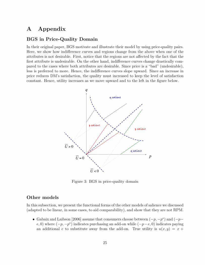
A Appendix

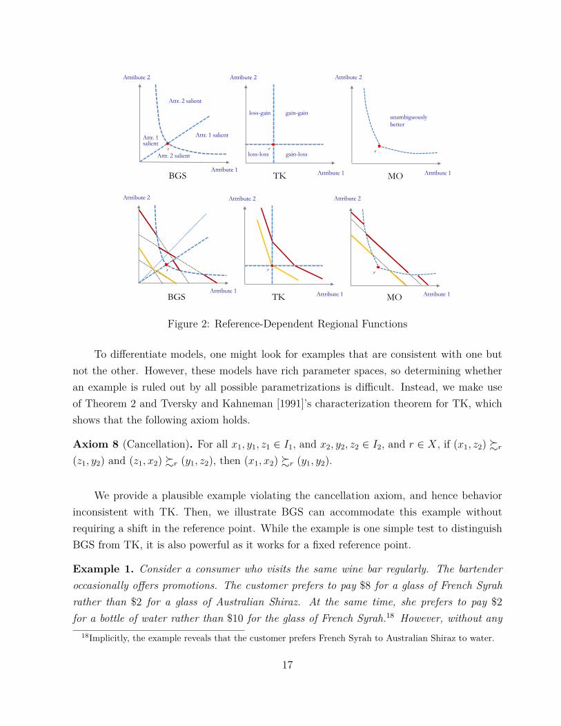
BGS in Price-Quality DomainIn their original paper, BGS motivate and illustrate their model by using price-quality pairs.Here, we show how indifference curves and regions change from the above when one of theattributes is not desirable. First, notice that the regions are not affected by the fact that thefirst attribute is undesirable. On the other hand, indifference curves change drastically com-pared to the cases where both attributes are desirable. Since price is a “bad” (undesirable),less is preferred to more. Hence, the indifference curves slope upward. Since an increase inprice reduces DM’s satisfaction, the quality must increased to keep the level of satisfactionconstant. Hence, utility increases as we move upward and to the left in the figure below.

q salient

p

q

q salient

p salient

U > 0

U = 0

U < 0

p salient

Figure 3: BGS in price-quality domain

Other modelsIn this subsection, we present the functional forms of the other models of salience we discussed(adapted to be linear, in some cases, to aid comparability), and show that they are not RPM.

• Gabaix and Laibson [2006] assume that consumers choose between (−p, −p∗) and (−p−e, 0) where (−p, −p∗) indicates purchasing an add-on while (−p−e, 0) indicates payingan additional e to substitute away from the add-on. True utility is u(x, y) = x +

25

y. Sophisticated agents and informed myopic agents maximize u, while uninformedmyopic agents maximize uM(x, y) = x.

• Kőszegi and Szeidl [2013] and Bushong et al. [2015] assume that the DM maximizes

U(x, C) = g1(C)x1 + g2(C)x2

where C is the comparison set, fixed per decision problem, and

gi(C) = g(

maxy∈C

yi − miny′∈C

y′i

).

The difference is in the properties that g satisifies. Kőszegi and Szeidl [2013] requireg′(x) > 0 for all x > 0. Bushong et al. [2015] require g′(x)x + g(x) > 0 and g′(x) < 0for all x > 0.

• Bhatia and Golman [2013] assume that the DM chooses the bundle x that maximizes

U(x|r) = α1(r1)[V (x1) − V (r1)] + α2(r2)[V (x2) − V (r2)]

given that a reference point r, where each αi is increasing and positive.

• Gabaix [2014] assumes a rational DM would maximize u(a, w) but actually maximizes

u (a, (w1m∗1, . . . , wnm∗

n))

wherem∗ ∈ arg min

m∈[0,1]n12

∑i,j

(1 − mi)Λij(1 − mj) + κ∑

i

mαi

where Λij incorporates the “variance” in the marginal utility of dimensions i and j.When n is large, m∗

i is often zero, so (w1m∗1, . . . , wnm∗

n) is a “sparse” vector.

All of the above fail to be RPM as the indifference curves have the same slope everywherefor a fixed reference point or reference set; indeed, Gabaix and Laibson do not incorporatea reference point at all.

Proof of Theorem 1Proof. First, we show the regional affine representation for each reference f . Second, weextend it across frames. To save notation, until Lemma 8, we fix f and write Ri instead ofRi(f) and % instead of %f .Lemma 1. For each Ri, there is an affine and increasing vi : Ri → R so that for x, y ∈ Ri,x % y ⇐⇒ vi(x) ≥ vi(y).

Proof. For each Ri, pick arbitrary xi ∈ Ri and εi > 0 s.t. Bεi(xi) ⊂ Ri. Bεi

(xi) is a mixturespace and % satisfies the mixture space axioms when restricted to it, so let it have the

26

representation vi, normalized so that vi(xi) = 0. Define vi by vi(x) = 1αvi(xαxi) for any

α ∈ (0, 1] so that xαxi ∈ Bεi(xi). To see vi is well defined, suppose xαxi, xβxi ∈ Bεi

(xi) and(WLOG) β < α. Then, xβxi = (xαxi)β

αxi, and since vi is affine, 1

βvi(xβxi) = 1

αvi(xαxi).

Lemma 2. If xi ∈ Ri, xj ∈ Rj, and xi ∼ xj, then there is α > 0, β ∈ R such that for x ∈ Ri

and y ∈ Rj, x % y ⇐⇒ vi(x) ≥ αvj(y) + β.

Proof. WLOG, take vi(xi) = 0. As above, there is εi such that Bεi(xi) ⊂ Ri. By Regional

Continuity (RC) and Monotonicty (RM), there is εj > 0 such that Bεj(xj) ⊂ Rj and for all

y ∈ Bεj(xj), x∗ = xi + εi �r y �r xi − εi = x∗; let ε = min εk. For any y ∈ Rj(r) and α such

that yαxj ∈ Bε(xj), there exists β ∈ (0, 1) such that x∗βx∗ ∼r yαxi by RC, RM, and WeakOrder. Let Vj(y) = α−1vi(x∗βx∗). This is well defined for the same reason as above, and isalso affine, increasing, and ranks alternatives in the same way as vj. Thus, Vj(y) = avj(y)+bfor a > 0 and b ∈ R.

For any x ∈ Ri and y ∈ Rj, pick α such that xαxi ∈ Bε(xi) and yαxj ∈ Bε(xj). Byconstruction, yαxj ∼ y′ when y′ ∈ Bε(xi) and vi(y′) = αVj(y). Thus, xαxi % y′ ∼ yαxj

holds if and only if vi(x) ≥ Vj(y) and x % y ⇐⇒ xαxi % yαxj, completing the proof.

Definition 6. A finite sequence Q1, ..., Qm with Qi ∈ {R1, ..., Rn} is an indifference sequence(IS) if there exists x1, ..., xm, y1, ..., ym with xj ∈ Qj, yj ∈ Qj+1 and xj ∼ yj. The functionv is a utility for the IS Q1, ..., Qm if v is affine and increasing on each Qi and for all i,x, y ∈ Qi

⋃Qi+1: x % y ⇐⇒ v(x) ≥ v(y).

For an IS Q1, ..., Qn with utility v, label v(Qi) = (li, ui). Note that we allow Qi = Rj

and Qk = Rj for i 6= k.Lemma 3. For an indifference sequence Q1, ..., Qn, there is an affine, increasing utility vfor it.

Proof. By Lemma 2, there is αi, βi such that x % y ⇐⇒ vi(x) ≥ αivi+1(y) + βi for allx ∈ Ri and y ∈ Ri+1. For any x ∈ Qi for i = 1, ..., n, define

v(x) =i−1∏j=1

αj vi(x) +i−1∑j=1

j−1∏k=1

αkβj.

When x, y ∈ Ri+1⋃

Ri, Lemma 2 implies that x % y ⇐⇒ v(x) ≥ v(y).

Lemma 4. Fix an IS Q1, ..., Qn with utility v. If xj ∈ Qj for j = i, i + 1, i + 2 withxi ∼ xi+1 ∼ xi+2, then Q1, ..., Qi, Qi+2, ..., Qn is an IS (after relabeling) with utility v.

Proof. The Lemma is vacuously true for any 1 or 2-element IS. Fix an IS Q1, ..., Qn withn ≥ 3 and v as above, and suppose xj ∈ Qj for j = i, i + 1, i + 2 with xi ∼ xi+1 ∼ xi+2.By transitivity xi ∼ xi+2, so Q1, ..., Qi, Qi+2, ..., Qn is an IS; it remains to be shown that vis a utility for it. There is an ε > 0 s.t. B = Bε(v(xi))) ⊂ (lj, uj) for j = i, i + 1, i + 2. Letv−1(u) : B → Qi+1 be an arbitrary point in Qi+1 such that v[v−1(u)] = u. Now, fix x ∈ Qi

27

and y ∈ Qi+2. For α small enough, v(xαxi), v(yαxi+2) ∈ B. Then xαxi ∼ v−1(v(xαxi)) andyαxi+2 ∼ v−1(v(yαxi+2)). So

x % y

⇐⇒ xαxi % yαxi+2

⇐⇒ v−1(v(xαxi)) % v−1(v(yαxi+2))⇐⇒ v[v−1(v(xαxi))] ≥ v[v−1(v(yαxi+2))]

⇐⇒ αv(x) + (1 − α)v(xi) ≥ αv(y) + (1 − α)v(xi+2)⇐⇒ v(x) ≥ v(y)

This establishes the Lemma.

Lemma 5. Fix an IS Q1, ..., Qn with utility v. If (l1, u1)⋂(ln, un) 6= ∅, then there exists i

and xj ∈ Qj for j = i + 1, i + 2, i + 3 with xi ∼ xi+1 ∼ xi+2.

Proof. If there is i with (li, ui)⋂(li+2, ui+2) 6= ∅, then there is u ∈ ⋂

j=i,i+1,i+2(lj, uj) so thereexists xj ∈ Qj with v(xj) = u for j = i, i + 1, i + 2 and thus by hypothesis, xi ∼ xi+1 ∼ xi+2.We show there exists such an i by contradiction. If li+2 > ui for all i or li > ui+2 for all i,then (l1, u1)

⋂(ln, un) = ∅, a contradiction. So there must exist i such that [li+2 > ui andli+2 > ui+4] or [ui+2 < li and ui+2 < li+4]. In the first case, li+2 ∈ (li+1, ui+1)

⋂(li+3, ui+3); inthe second, ui+2 ∈ (li+1, ui+1)

⋂(li+3, ui+3). In either case, we have a contradiction.

Lemma 6. Fix an IS Q1, ..., Qn with utility v. Then for all x, y ∈ ⋃i Qi, x % y ⇐⇒ v(x) ≥

v(y).

Proof. This is clearly true if n = 1. (IH) Suppose the claim is true for any IS with m < nelements. Fix an IS Q1, ..., Qn with utility v. If x /∈ Q1

⋃Qn or y /∈ Q1

⋃Qn, then the claim

immediately follows from the IH, and clearly holds if x, y ∈ Qi for some i. So it suffices toconsider arbitrary x ∈ Q1 and y ∈ Qn. By Lemmas 4 and 5, if (u1, l1)

⋂(ln, un) 6= ∅, we canform a shorter IS from Q1 to Qn and the claim then follows from the IH.

There are two cases to consider: ln > u1 and un < l1. If ln > u1, then there existsy′ ∈ Qn′ for n′ < n with v(y′) = ln. By the IH, that Q1, ..., Qn′ is an IS and v(y′) > v(x),y′ � x. Similarly, since Qn′ , ..., Qn is an IS and v(y) > v(y′), y � y′. By transitivity, y � xand since v(y) > ln > u1 > v(x), the claim holds. Similar arguments obtain the desiredconclusion when un < l1.

Define the relation ∼= by x ∼= y ⇐⇒ there exists an IS Q1, ..., Qm with x ∈ Q1 andy ∈ Qm. It is easy to see that ∼= is an equivalence relation (reflexive and transitive). Let [x]denote the ∼= equivalence class of x.Lemma 7. If y /∈ [x] and x � y, then x′ � y′ for all x′ ∈ [x] and y′ ∈ [y].

Proof. Fix x, y ∈ X with y /∈ [x] and x � y, and assume x ∈ Rk Pick any y′ ∈ [y]. Bydefinition, there is an IS Q1, ..., Qm with y′ ∈ Qm and y ∈ Q1. Let i = 1 any y1 = y. If thereexists y′′ ∈ Qi with y′′ % x, then y′′ % x � yi, so by RC and connectedness of Qi, we can find

28

z ∈ Qi with z ∼ x. If that occurs, then Rk, Qi, ..., Q1 is an IS and y ∈ [x], a contradiction.Thus x � y′′ for all y′′ ∈ Qi. Moreover, there exists yi+1 ∈ Qi+1 with x � yi+1 by transitivityand definition of IS, so we can apply above logic to Qi+1 as well. Inductively, x � y′. Sincey′ is arbitrary, this extends to any y′ ∈ [y]. Similar arguments show that x′ � y for anyx′ ∈ [x]. Combining, x′ � y′ whenever x′ ∈ [x] and y′ ∈ [y].

Let A1, ..., An be the distinct equivalence classes of ∼=. By Lemma 7, these sets can becompletely ordered by �, i.e. Ai � Aj ⇐⇒ x � y for all x ∈ Ai and y ∈ Aj. WLOG,A1 � A2 � ... � An.

By Lemma 6, there is vi on Ai so that vi is affine and increasing on region contained inAi and x % y ⇐⇒ vi(x) ≥ vi(y) for all x, y ∈ Ai. Note that vi(Ai) is bounded for all i > 1.Define V (x) = v1(x) for all x ∈ A1. For x ∈ Ai with i > 1, define and V (x) recursively by

V (x) = vi(x) − supy∈Ai

vi(y) + infy∈Ai−1

V (y) − 1

Observe V (·) is a positive affine transformation of vi(·) on Ai and if x ∈ Ai, y ∈ Aj andi > j, then V (x) > V (y). Thus V represents % and is affine and increasing when restrictedto any given region.

Up to now, we fixed f ∈ F and constructed a representation for %f . Since f is arbitrary,this establishes that each %f has a representation V (·|f) that is affine and increasing on Ri(f)for i = 1, ..., n. Denoting uj(·|f) the restriction to Rj(f), we have established the existenceof an RPM if uj(·|f ′) is a positive affine transformation of uj(·|f) for any f, f ′.Lemma 8. For i = 1, ..., n and all f, f ′ ∈ F , there are α > 0 and β ∈ R so that ui(·|f ′) =αui(·|f) + β.

Proof. Write u ≈ v if there are α > 0 and β ∈ R so that u = αv + β. Pick any f ∈ F andlet

E = {e ∈ F : ui(·|e) ≈ ui(·|f)}.

E is closed, since if en ∈ E and en → e ∈ F , then for any open ball B ⊂ Ri(e), Ri(en) ⋂B 6= ∅

for n large enough by lower semicontinuity of Ri. Observe B′ = Ri(en) ⋂B ⊂ Ri(en) ⋂

Ri(e)is a mixture space and FI plus the usual uniqueness argument for affine utility functionsgives that ui(·|en) ≈ ui(·|e). Now, consider E ′ = cl(Ec). If E ′ ⋂

E 6= ∅, then the sameargument as above with a sequence in Ec converging to e ∈ E yields a contradiction. HenceE ′ ⋂

E = ∅ and E⋃

E ′ = F . Since F is connected, E ′ = ∅ and E = F .

Thus ui(·|f) is an affine transformation of ui(·|f ′) for all f, f ′ ∈ F and {%f} conformsto RPM under R.

Proof of Proposition 1Proof. Note first that if there is no non-empty open set with this property, then the largestset revealed part of the region around x is ∅. Otherwise, we show there is a largest set usingZorn’s lemma. Let At∈T be a chain of open sets revealed part of the region around x, ordered

29

by ⊆. We claim that ⋃t∈T At = B is an upper bound and also revealed part of the region

around x. As a union of open sets, it is clearly open. If a, b, aαc, bαc ∈ B, then there areta, tb, taαc, tbαc so that a ∈ Ata , b ∈ Atb

, etc. Let At∗ be the ⊆-maximum of the four. Thena, b, aαc, bαc ∈ At∗ . It follows that a %r b ⇐⇒ aαc %r bαc. Thus there is at least one⊆-maximal element.

Clearly Ri(r) is a revealed region around x when x ∈ Ri(r). Assume ui(·|r) is not apositive affine transformation of uj(·|r) whenever i 6= j. If the result is false, then A is arevealed region around x and there exists y ∈ A \ Ri(r). There is a region Rj(r), j 6= i, suchthat y ∈ Rj(r) or, since A is open and ⋃n

j=1 Rj(r) is dense, there is Rj(r) y′ ∈ A \ R−i(r).WLOG, assume the former. Then there exists z ∈ A

⋂Rj(r) \ y such that y ∼r z. However,

for β > 0 small enough, yβx, zβx ∈ Ri(r). But by assumption, the slope of the indifferencecurves in Ri differs from that of Rj. Thus we have yβx 6∼r zβx, a contradiction of A beinga revealed region.

Proof of Proposition 2Proof. First, we show (i) =⇒ (ii). Set σ(a, b) = max{a/b, b/a}. Clearly σ is a saliencefunction. Fix f and set A = {x : σ(x1, e1) > σ(x2, e2)}. We show A = R1(e).

Claim A⋂

R2(e) = ∅. If not, pick x ∈ A⋂

R2(e). x ∈ A implies either (a) x1/e1 > x2/e2and x1/e1 > e2/x2 or (b) e1/x1 > x2/e2 and e1/x1 > e2/x2. If (a) and x2 ≥ e2, then

x1 ≥ e1e2/x2 > e1,

so there exists λ ∈ (0, 1] such that (λx1 + (1 − λ)e1, x2) = (e1e2/x2, x2) = x′. If (a) andx2 < e2, then

x1 > e1x2/e2 > e1,

so there exists λ ∈ (0, 1) such that (λx1 + (1 − λ)e1, x2) = (e1x2/e2, x2) = x′. By moderationand x ∈ R2(e), x′ ∈ R2(e). However, x′

1x′2 = e1e2 or x′

1/x′2 = e1/e2 so x′ /∈ R2(e) by equal

salience, a contradiction. A similar contradiction obtains if (b) holds.Now, since A

⋂R2(e) = ∅ and R1(e) ⋃

R2(e) is dense, A ⊂ cl(R1(e)). By SmoothRegions, R1(e) =

∫cl(R1(e)). Thus A ⊆ R1(e). Similarly, for B = {x : σ(x1, e1) <

σ(x2, e2)}, B ⊆ R2(e). But

(A⋃

B)c = {x : x1x2 = e1e2 or x1/x2 = e1/e2}⋂

(R1(e)⋃

R2(e)) = ∅.

Thus A = R1(e) and B = R2(e), completing the proof.Now, we show (ii) implies (i). First, moderation follows from ordering. Second, equal

salience follows from symmetry and homogeneity of degree zero. Third, Smooth Regionsfollows from continuous σ.

Finally, to see (iii) if and only if (ii), fix any salience function s. Observe s(a, b) >s(c, d) iff s(a/b, 1) > s(c/d, 1) by homogeneity iff s(max(a/b, b/a), 1) > s(max(c/d, d/c), 1)by symmetry iff max(a/b, b/a) > max(c/d, d/c) by ordering. Thus any salience function isequivalent.

30

Proof of Proposition 3Proof. Necessity is obvious, so assume Axioms 1-4 and SFI. By Theorem 1, there exists aRPM.20 Without loss of generality, normalize so that u1(·|r) = u1(·|r′) for all r, r′. Observethat ui(Ri(r)|r) ⋂

uj(Rj(r)|r) 6= ∅ for all r. Suppose ui(·|r) 6= ui(·|r′) for some r, r′ andsome i. Then, let ε = d(r, r′) and pick a sequence rn → r such that: ui(·|rn) 6= ui(·|r)and d(rn, r) → inf{d(r′, r) : ui(·|r) 6= ui(·|r′)}. Similarly, let rn be a sequence such thatrn → r and ui(·|r) = ui(·|rn). By each Ri(r) is open, there exists ε, xi and x1 such thatBε(xi) ⊂ Ri(r), Bε(x1) ⊂ R1(r), and xi ∼r x1. By continuity of the region functions,Bε(xi) ⊆ Ri(rn) ⋂

Ri(rn) and Bε(x1) ⊆ R1(rn) ⋂R1(rn) for n large enough. For z close

enough to xi, there exists y(z) ∈ Bε(x1) such that z ∼r y(z). But then by SFI, z ∼rn y(z)and z ∼rn y(z). Thus ui(z|rn) = u1(y(z)|rn) = u1(y(z)|rn) = ui(z|rn) for all z close enoughto xi, implying that ui(·|rn) = ui(·|rn), a contradiction. Conclude ui(·|r) = ui(·|r′) for allr, r′.

Proof of Theorem 2Lemma 9. For any r, there exists xi ∈ Ri(r) for i = 1, 2 with x1 ∼r x2.

Proof. We first show the result for r = (z, z). Let Rzi = {x ∈ Ri(a) : x1x2 < z2}, the points

in Ri(r) above the Cobb-Douglas line passing through r. Pick a ∈ Rz1 and b ∈ Rz

2. If a �r b,then by reflection and S1-S3, a′ �r b′ when a′ = (a2, a1) ∈ Rz

2 and b′ = (b2, b1) ∈ Rz1. A

simple proof using completeness, transitivity, RC and that both Rz1, Rz

2 open and connectedyields xi ∈ Ri(r) for i = 1, 2 with x1 ∼r x2. Similar proofs hold if a ∼r b or b �r a.

Note the above arguments are true for Rz′i when z′ < z, since Rz′

i ⊂ Rzi ⊂ Ri(r).

Within each Rzi , indifference curves are linear, parallel and downward sloping by RL and

RM. For z′ to be close 0, the x1, x2 we find must lie on indifference curves that intersect theboundary without leaving Rz

i . Thus for any r′, we can find x′1 and x′

2 so that xi ∼r x′i and

xi, x′i ∈ Ri(r) ⋂

Ri(r′) for i = 1, 2. But then by SFI and transitivity, x′1 ∼r′ x′

2.

Proof. By the Lemma, we can apply Proposition 3. Hence there are u1, u2 such that ifx ∈ Ri(r) and y ∈ Rj(r), then x %f y ⇐⇒ ui(x) ≥ uj(y). Now, ui(x) = aix1 + bix2 + ci,and c1 = 0 WLOG. RM implies ai, bi > 0.

Fix arbitrary r = (r1, r2) and let r′ = (r2, r1). For any distinct x, y ∈ R1(r) suchthat x ∼ y, a1x1 + b1x2 = a1y1 + b1y2. By reflection and the structure of R, we have(x2, x1), (y2, y1) ∈ R2(r′) and (x2, x1) ∼r′ (y2, y1). Hence, a2x2 + b2x1 + c2 = a2y2 + b2y1 + c2

and b2/a2 = (y1 − x1)/(x2 − y2) and (x1 − y1)/(y2 − x2) = a1/b1, so there exists α > 0 suchthat b2 = αa1 and b1 = αa2.

For contradiction, suppose α 6= 1. Pick (x, y) ∈ R1(1, 1) and (a, b) ∈ R2(1, 1) so that(x, y) ∼1,1 (a, b). Note (b, a) ∈ R1(1, 1) and (y, x) ∈ R2(1, 1). By Reflection, (y, x) ∼1,1 (b, a).

20By SFI, there is a point of indifference between all regions so a disconnected region is not problematic.

31

Then

a1x + b1y = α[a1b + b1a] + c2

a1b + b1a = α[a1x + b1y] + c2

a1b + b1a = α[α[a1b + b1a] + c2] + c2

a1b + b1a = α2[a1b + b1a] + (1 + α)c2

(1 − α2)[a1b + b1a] = (1 + α)c2

Since we can find similar indifferences for any bundles in a small enough neighborhood of(a, b), this requires α = 1. Now, the first two equalities imply

a1b + b1a = [[a1b + b1a] + c2] + c2

and so c2 = 0.After a normalization, we have u1(x) = wx1 + (1 − w)x2 and u2(x) = (1 − w)x1 + wx1.

To conclude, we must show w > 12 . Pick any y ∈ (0, x). Consider the line L(y) = {x′ ∈ X :

u2(x′) = u2(y, y)}. This is the line with slope −w1−w

that intersects the 45-degree line at (y, y).For any x ∈ L(y) such that x1 > y > x2, we can find r, r′ so that (y, y) ∈ R2(r) ⋂

R2(r′),(x1, x2) ∈ R2(r) ⋂

R1(r′). By construction (x1, x2) ∼r (y, y), so since x1 > x2, by SDO wehave (x1, x2) �r′ (y, y) and wx1 +(1−w)x2 > y = (1−w)x1 +wx2. Letting (x1, x2) → (y, y)gives taht w > 1

2 .

Proof of Proposition 4Proof. By Proposition 3, drop the dependence on r and write ui(·) instead of ui(·|r). LetUi = {x ∈ X : ui(x) > uj(x)∀j 6= i} and Li = {x ∈ X : ui(x) < uj(x)∀j 6= i}. DefineR−i(r) = ⋃

j 6=i Rj(r).Lemma 10. If %r satisfies Monotonicity and z ∈ Ui

⋂Ri(r), then R−i(r) ⋂{x : x �

z} ⋂Ui = ∅.

Proof. Suppose not, so there is z ∈ Ui⋂

Ri(r) such that A = R−i(r) ⋂{x : x � z} ⋂Ui 6= ∅.

Then let yn be a sequence of points in A approaching as close as possible to z. WLOG, yn → y(since yn must eventually belong to the compact set Bε(z) for some ε > 0). Then we can pickxn ∈ Ri(r) ⋂{y : y ≤ y} that converges to y ∈ bd(Ri(r)).21 Noting u−i(x) = maxj 6=i uj(x) iscontinuous,

lim ui(xn) = ui(y) > u−i(y) = lim u−i(yn)

and so xn �r ym for n, m large enough, but ym ≥ xn by taking n large enough that d(xn, y)) <d(ym, y). This contradicts Monotonicity.

Lemma 11. If %r satisfies Monotonicity and r ∈ Ui, then R−i(r) ⋂{x : x � r} ⋂Ui = ∅.

21If y = r, then take xn = r for all n; otherwise, d(x′, r) < d(y, r) implies x′ ∈ Ri(r).

32

Proof. Follows from applying Lemma 10 to a sequence xn in Ri(r) that converges to r.

Lemma 12. If %r satisfies Monotonicity and z ∈ Li⋂

Ri(r) then R−i(r) ⋂{x : x �z} ⋂

Li = ∅.

Proof. Dual to Lemma 10.

Lemma 13. If %r satisfies Monotonicity and r ∈ Li, then R−i(r) ⋂{x : x � r} ⋂Li = ∅.

Proof. Follows from applying Lemma 12 to a sequence xn in Ri(r) that converges to r.

By salience utilities, there are i and j so that Ui = Lj = {(x1, x2) : x2 ≤ x1} andUj = Li = {(x1, x2) : x2 ≥ x1}; without loss of generality, let i = 1 and j = 2. Pickr0 ∈ X so that u1(r0) = u2(r0); such a point exists because (x, x) ∈ X. Note that {x :u1(x) = u2(x)} is an upward sloping line, and for ε > 0, u1(r0 − (0, ε)) > u2(r0 − (0, ε)) andu2(r0 + (0, ε)) > u1(r0 + (0, ε)). Noting U1 = L2 and U2 = L1, by the Lemmas and that theregions are dense:

cl(R1(r0 − (0, ε))) ⊇ {x ∈ U1 : x � r0 − (0, ε)}cl(R2(r0 + (0, ε))) ⊇ {x ∈ U2 : x � r0 + (0, ε)}cl(R1(r0 + (0, ε))) ⊇ {x ∈ L1 : x � r0 + (0, ε)}cl(R2(r0 − (0, ε))) ⊇ {x ∈ L2 : x � r0 − (0, ε)}

Letting ε → 0 and applying continuity of each Ri, cl(R1(r0)) ⊇ {x ∈ U1 : x � r0}⋃{x ∈

U2 : x � r0} and cl(R2(r0)) ⊇ {x ∈ U1 : x � r0}⋃{x ∈ U2 : x � r0}.

For all r close enough to r0, Rk(r) ⋂Uk 6= ∅ and Rk(r) ⋂

Lk 6= ∅ for k = 1, 2. Pick suchan r that also belongs to U1. By the above, Ri(r) intersects Uk and Lk for all i, k ∈ {1, 2}.⊇ {x ∈ U1 : x � r} ⋃{x ∈ U2 : x � r}.

Pick y ∈ R2(r) ⋂U2. In Rn, connected is equivalent to path connected, so there is a

continuous function θ : [0, 1] → R2(r) ⋃{r} with θ(0) = y and θ(1) = r. There must existz0 such that θ(z0) ∈ {x : u1(x) = u2(x)}. Because R2(r) is open, there exists ε > 0 s.t.Bε(θ(z0)) ⊂ R2(r). Observing that Bε(θ(z0)) intersects both L2 and U2, by Lemmas 10and 12, R1(r) intersects neither {(θ(z0)1, z) : z ∈ R+} nor {(z, θ(z0)2) : z ∈ R+}. Thiscontradicts connectedness of R1(r).

Proof of Proposition 5Proof. By Theorem 1 and salient thinking, we can apply Proposition 3 to get a RD-RPMrepresentation with ui(·|r) = ui(·). There exists a, b ∈ R2

++ and c ∈ R such that u1(x) =a · x + b and u2(x) = b · x, perhaps after a normalization. Let r be arbitrary and thenpick x, x′, x′′ ∈ R1(r) and y, y′, y′′ ∈ R2(r) as in the definition of salient thinking. Then,u1(x) = u2(y). Hence, a1ε1 = u1(x′) − u1(x) > u2(y′) − u2(y) = b1ε1, and b2ε2 = u2(y′′) −u2(y) > u1(x′′) − u1(x) = a2ε2. Conclude a1 > b1 and a2 > b2.

If there exists x∗ where u1(x∗) = u2(x∗), then a violation of Monotonicity follows from re-placing (x, x) with x∗ in the same arguments establishing Proposition 4. Since X is connected

33

and u1(·)−u2(·) is a continuous function, either u1(x) > u2(x) for all x ∈ X or u2(x) > u1(x)for all x ∈ X. Set i such that ui(x) > u−i(x) for some x ∈ X. Then Lemmas 10 and 12establish that cl(Ri(r)) = ⋃

x∈cl(Ri(r)){y : y ≥ x} and cl(Rj(r)) = ⋃x∈cl(Rj(r)){y : y ≤ x}.

34