A Regime-Switching Heston Model

for VIX and S&P 500 Implied Volatilities

Andrew Papanicolaou∗ Ronnie Sircar†

October 2012, revised April 25, 2013

Abstract

Volatility products have become popular in the past 15 years as a hedge against market uncer-tainty. In particular, there is growing interest in options on the VIX volatility index. A number ofrecent empirical studies examine whether there is significantly greater risk premium in VIX optionprices compared with S&P 500 option prices. We address this issue by proposing and analyzing astochastic volatility model with regime switching. The basic Heston model cannot capture VIX im-plied volatilities, as has been documented. We show that the incorporation of sharp regime shifts canbridge this shortcoming. We take advantage of asymptotic and Fourier methods to make the extensiontractable, and we present a fit to data, both in times of crisis and relative calm, which shows theeffectiveness of the regime switching.

1 Introduction

Volatility derivatives have become popular at least since 1998, primarily through variance swaps. Morerecently, they have been viewed as indicators of the market’s perception and quantification of futureuncertainty. The VIX volatility index has become a household name as the “fear index”. We present,analyze, and test to data a stochastic volatility model with regime switching that tries to capture the“spike-o-phobia” that seems apparent in the pronounced skew of the VIX options implied volatilitysurface.

Stochastic volatility jump-diffusion models are known to be effective in fitting the implied volatility ofS&P 500 (SPX) options. However, VIX options cannot be fit by the widely-used Heston model becausemany of the strikes lie in the tail of the volatility process’s distribution. Therefore, a model for consistentpricing of both VIX and SPX options should have a volatility process that has a distribution whichspreads probability mass over a broader range than the standard square-root process. In this paper wepropose the addition of a regime-switching process to the Heston model, a modeling feature that willwiden the support of the bulk of the volatility process’s probability distribution. The fits to data arequalitatively reasonable, but there is some disparity between the two markets, a finding also reported inrecent econometric literature that we discuss below.

The Heston model is an industry standard among stochastic volatility models. Its parameters areknown to have clear and specific controls on the implied volatility skew/smile, and it can mimic theimplied volatilities of around-the-money options with a fair degree of accuracy. A major shortcoming is

∗ORFE Department, Princeton University, Sherrerd Hall, Princeton NJ 08544, apapanic@princeton.edu. Work partiallysupported by NSF grant DMS-0739195.†ORFE Department, Princeton University, Sherrerd Hall, Princeton NJ 08544, sircar@princeton.edu. Work partially

supported by NSF grant DMS-1211906.

1

that it is often unable to fit the implied skew of short-time-to-maturity options. Nevertheless, it is stillwidely used, and so it would be significant (both in practice and in theory) if it was shown that additionalfeatures such as jumps and regime-change allow it to effectively price VIX derivatives.

The formula for the price of a European call option in the Heston model was originally derived in[25], formulae for jump models are given in [28], and combined jump-diffusion models are analyzed in[2, 19]. In particular, a square-root process with jumps in both the underlying and the volatility was usedin [32] to price VIX options. However, several studies have shown that VIX implied volatility data is notreproducible by models with volatility given by a square-root process [16, 23, 31]. Alternative models suchas the 3/2-model have emerged as possible candidates for fitting VIX implied volatility [3, 15]. Anotherapproach is to take VIX options or variance swap data directly into the model of the underlying S&P 500index (SPX) so that it is consistent by design, but at the cost of the index dynamics depending on thematurity dates of the volatility derivatives. This is the market model approach taken in [13]. In [30], asimultaneous fit to VIX and SPX option prices is presented using Sato processes. Recently, [4] presentsjoint fits using a double mean-reverting diffusion model using Monte Carlo simulation.

However, there are several empirical papers that focus on the quality of the fits achieved. For instance[14] demonstrates the difficulty of fitting out of the money VIX options well, while [12] finds that “theinformation content implied from these two option markets is not identical”. In a current working paper,[33] use nonparametric estimates of state price densities implied from SPX and VIX option marketsand find that “VIX options deliver unique information for investors to extract information on volatilitydynamics”. In many ways, the issues are how one interprets consistency and quality of fits, particularly ifone demands good fits across all strikes and even short maturities, and the mixed message reflects morethe practitioner or econometrics perspective of the authors.

In the time series literature, markets with Markov regime change were studied in [24], the importanceof identifying regime change for GARCH models was identified in [26], and the importance of jumpswas highlighted in [1, 5, 34, 31], where evidence from variance swap data suggests that fears regardingoutlier events creates a premium that is most likely caused by jump risk. Elliott et al. [10, 11] proposean extended Heston model, where the parameters in the volatility process are modulated by a Markovchain, and they analyze the pricing of variance swaps and other derivatives. They demonstrate theimpact of regime change by Monte Carlo experiments, but they did not consider VIX options valuationor calibration to data as we do here.

In this paper, we specify a parametrically richer version of the Heston wherein the volatility processis modulated by a Markov chain that represents the regime state of the market’s volatility. The modelalso has a jump structure that depends on the regime change in such a way as to model the contrarymotion between equity and volatility (i.e. the leverage effect). The rate of regime-change is taken to beof a small enough order so that option prices can be expanded with a power series. In this expansion,the lowest order term is the Heston model’s price and the first correction term can also be written as afunction of the components of the Heston price. This is similar to the methodology in [20], except thatthey have added a fast-mean reverting diffusion to the Heston model whereas we have added a slow jumpfactor. In both their paper and ours, there are explicit formulae for the Fourier transform of the optionprice’s expansion.

When applied to data, we find that our model captures separately the implied volatility skews of boththe SPX and VIX options (see Figures 6 and 7). But when the parameter estimates from VIX optionsare used to compute SPX option prices through the model, some systematic discrepancies between thetwo markets are revealed (see Figure 8), which highlights a distinction between the the VIX and SPXoptions markets. We also apply the model to VIX options from the 2008 financial crisis and to non-crisisdata of 2011, and are able to relate the parameter estimates to the historical beliefs about volatility fearsduring these periods

The rest of the paper is organized as follows: Section 2 provides an introductory analysis of the VIX

2

and SPX time series data, along with some analysis of the implied volatility of VIX options; Section 3describes the model that we’re proposing, as well as the derivation of some key items such as the varianceswap rate, the VIX formula, and a PIDE for option pricing; Section 4 derives an expansion for solvingthe pricing PIDE, for both the case of stock options and VIX options; Section 5 describes the procedurefor calibrating the data to the pricing formulae (both for VIX and SPX options data) and also providesan empirical study of 2008 crisis data and some post-crisis data; Section 6 concludes.

2 Preliminary Data Analysis

To motivate our choice of model, we start by examining the market data. We’ll look at time series dataand the VIX options implied volatility skew; these empirical facts will give us some bearing on whichfeatures are important.

2.1 Time Series Analysis

Figure 1 shows the time-series plot of the SPX index and the VIX. It is well-known that a volatility

Figure 1: The solid line is the time series plot of the SPX index, and the dotted line is the VIX index. Thecorrelation of these time series is about −80%.

leverage effect needs to be included in any useful model, and indeed, from the figure we can see an inverserelationship between the SPX and the VIX: bull markets are accompanied by low VIX, and bear marketsare accompanied by higher VIX. Empirically, the negative correlation between log-returns on SPX andlog-returns on VIX is quite strong, usually around −60% to −80%. Furthermore, Figure 1 is interestingbecause it shows a time series over a period where the markets experience several macroeconomic shocks.There will be significantly higher correlation for time-windows with a couple of these shocks, compared

3

to that of time windows where there are no shocks. Hence, negative correlation between S&P 500 and theVIX should be modeled with two components: correlated diffusion processes to account for the day-to-daymicrostructure fluctuations, and a jump process to model the singular events that shock the market. Theimportance of jumps for describing the volatility leverage effect is found in [34].

Heavy tails are another important feature that can be deduced from the time-series. Figure 2 showsthe scatter plot of the log-returns on VIX against the log-returns on SPX, along with simulated returnssampled from various fits to bivariate distributions. It is clear from these scatter plots that simply fitting a

Figure 2: Top Left: The scatter plot of the log-returns on VIX against the log-returns on SPX. Top Right:Simulations from a fitted Gumbel copula. Bottom Left: Simulations from a fitted Gaussian copula. BottomRight: Simulations from a fitted bivariate Gaussian distribution. Notice that the bivariate Gaussian simulationdoes not have enough outliers.

bivariate Gaussian distribution to log-returns is insufficient, and that the bivariate distribution of returnscan be better-fitted with a copula. The copula fits in Figure 2 suggest that not only should there benegative correlation between the log-returns of SPX and VIX, but there should also be jumps in bothindices and these jumps should happen in opposite directions.

4

2.2 VIX Option Implied Volatility

For two times t and T with t ≤ T <∞, denote the future on VIX at time t with settlement date T as

Ft,T = EtVIXT

where Et is the expectation under the market-chosen risk-neutral measure. The payoff on a VIX calloption is (FT,T −K)+, and so the Black model for pricing an option on Ft,T can be applied::

CBS(Ft,T , T − t, r,K, σ) = e−r(T−t) (Ft,TN (d1)−KN (d2))

d1 =log(Ft,T /K) + σ2

2 (T − t)σ√T − t

d2 = d1 − σ√T − t ,

where N (·) denotes the CDF of the standard normal distribution function. The implied volatility of thisoption is σBSt (T,K) such that

CBS(Ft,T , T − t, r,K, σBSt (T,K)) = Cdatat (K).

Implied volatilities for VIX options on April 8th, 2011 are shown in Figure 3. Some things are importantto notice: there is a premium on low strike options as well as those with high strike; the low-point inthe curve moves to the left of the future price as time-to-maturity increases; the overall level of volatilitygoes down as time-to-maturity increases. But most importantly, one should take note of the increasein implied volatility as strike increases. In [15, 16, 23, 31], it is recognized that this increase in impliedvolatility is a phenomenon which cannot be described by the Heston model, the reason being that thesquare-root process has relatively little probability mass outside the range of everyday values. Hence,outlier events being hedged by high-strike VIX options are under-priced by the Heston model. A usefulmodel will have to account for this phenomenon.

3 Heston Model with Regime Change

We work on a probability space (Ω,F ,P) where P is a risk-neutral or equivalent martingale measure. Letθt be a continuous-time Markov chain that represents the regime-state of volatility. The regime variablecan take three values, θt ∈ 1, 2, 3 where θt = 1 means that volatility is in its low state, θt = 2means it is in medium state, and θt = 3 means it is in a high state. The probabilities of regime-changeare given by the intensity matrix Q ∈ R3×3, and the distribution of θt satisfies

d

dtP(θt = n) = δ

3∑m=1

QmnP(θt = m) for n = 1, 2, 3, (1)

where δ > 0 is a small parameter which creates a slow time scale in the regime. The log-price X of astock (or index) and its volatility follow paths generated by the following stochastic differential equations(SDEs):

dXt =

(r − 1

2f2(θt)Yt − δν(θt-)

)dt+ f(θt)

√Yt dWt − λ(θt)Jt dNt , (2)

dYt = κ(Y − Yt)dt+ γ√Yt dBt ,

dNt = 1[θt 6=θt−],

5

Figure 3: The implied volatilities of VIX call options (solid line) and put options (dotted line) on April 8th, 2011.The vertical black line is the future price with settlement data equivalent to the option expiry. Notice the higherimplied volatility on low strike options as well as those with high strike; the low-point in the curve moves to theleft of the future price as time-to-maturity increases; the overall level of volatility goes down as time-to-maturityincreases.

where r ≥ 0 is the risk-free rate of return, and Wt and Bt are Brownian motions with correlationρ ∈ (−1, 1) so that EdWt dBt = ρ dt. The random jump sizes Jt are independent and identicallydistributed as exponential with parameter 1. Both Jt and the regime process θt are independent of theBrownian motions and of each other. The function λ controls the direction and magnitude of jumps inthe stock price, and the function δν compensates the jumps so that eXt−rt is a martingale:

δν(n) = lim∆t0

E[∫ t+∆tt

(e−λ(θs)Js − 1

)dNs

∣∣∣θt− = n]

∆t= −

∑m 6=n

δQnmλ(m)

1 + λ(m),

for n = 1, 2, 3, using the moment generating function Ee−λ(m)Js = 11+λ(m) . Finally, parameters should be

chosen to satisfy the Feller condition, γ2 ≤ 2κY . This will ensure that Yt stays strictly positive.The Heston model is popular in pricing not only because it has an explicit (up to Fourier transform)

formula, but because it has a handful of parameters that can be identified with effects that are observedin equity implied volatilities. Some motivation for and features of our model are:

• The persistence of high volatility levels when there is a jump in the stock price. Historically,precipitous drops in asset prices have been accompanied by spikes in volatility, and this is preciselywhat is accomplished by having an exponential random variable that is amplified by λ(θt): when

6

volatility jumps to its high state there will be a drop in the stock price, and when volatility jumpsto its low state there will be a short-lived surge.

• The parameter δ and the matrix Q quantify the intensity with which the market views the possibilityof a change in the volatility state. Our assumption will be that δQ is of a relatively small orderso that we can do an asymptotic series expansion of equity options; our pricing formula for VIXoptions will be exact.

• The regime process controls the level of volatility in the strategy of the VIX tail hedge (VXTH),which is one of the CBOE’s indices for tracking the price of volatility risk. Volatility is consideredto be in a low state when the VIX future is between 15% and 30%; a medium state when the VIXfuture is between 20% and 50%; and a high state when the VIX future is over 50%.1

The model in (2) is fundamentally related to the jump models in [2] and [28], but the addition of theregimes and the additional structure in the jumps prevent us from pricing directly with an affine Fouriertransform. Also, model (2) is a mixture model, as the future distribution of XT and YT can be viewedas a mixture of three distributions, each of which is parameterized by a regime state.

3.1 Variance Swaps & the VIX

Volatility swaps, variance swaps and swaptions on realized variance are derivatives onXt that have becomeliquid in OTC markets over the past few decades (see [6] for a general review of volatility derivatives).They provide the investor with an instrument that returns a positive cash flow in times of high volatility.European call and put options on VIX have also become liquid, but these options are considerably exoticas they are really an option on a basket of S&P 500 options (the VIX is itself a basket of S&P 500 options;see [7, 8] or chapter 11 of [22]), and so pricing a European option on VIX is somewhat like pricing acompound option on the stock.

Let Et denote the risk-neutral expectation given the filtration Ft generated by (Xs, Ys, θs) : s ≤ t.For T > 0, the realized variance of the stock up to time T is the quadratic variation of its logarithm:

[X]T = lim‖T ‖0

∑t`∈T

(Xt`+1−Xt`)

2 where T is a partition of [0, T ] ,

which is referred to as the ‘floating-leg’ of a variance swap contract. For a variance swap contract occurringduring the period [t, t + τ ] for some τ > 0, the swap rate (or the ‘fixed-leg’) is given by the quadraticvariation of log(Xt) over the interval [t, t+ τ ]. Then we have

VSt,τ =1

τ(Et[X]t+τ − [X]t)

=1

τEt(∫ t+τ

tf2(θs)Ys ds+

∫ t+τ

tλ2(θs)J

2s dNs

)

=1

τ

∫ t+τ

tEt[f2(θs)Ys] ds+ 2δ

∑n,m 6=n

[I(t; τ)]θt,n λ2(m)Qnm

,

where we define the matrix I by

I(t; τ) =

∫ t+τ

t

[eδ(s−t)Q

]ds.

1There is a VXTH white paper located at http://www.cboe.com/micro/VXTH/documents/VXTHWhitePaper.pdf.

7

Therefore,

VSt,τ =Y

τ

∫ t+τ

tEt[f2(θs)] ds+

(Yt − Y )

τ

∫ t+τ

te−κ(s−t)Et[f2(θs)] ds+

2δ

τ

∑n,m 6=n

[I(t; τ)]θt,n λ2(m)Qnm. (3)

In contrast to variance swap rates, the volatility swap rate is the expectation of the square-root ofrealized variance and is considerably more model-dependent and harder to compute. Formulae can alsobe derived for the pricing of swaptions or options on realized variance (see [32]). We will not work withswaptions and volatility swaps in this paper; we have only introduced the variance swap rate because itis relevant in evaluating the VIX and is hence relevant in the pricing of VIX options.

3.1.1 Relationship between the Variance Swaps, the VIX and the Log Contract

Let VIXt denote the VIX index at time t (in hundredths of a decimal). The CBOE’s VIX index, as itwas re-furbished in 2002, is a discretization of the formula [6, 7, 8, 22],

VIXt =

√√√√2erτ

τ

(∫ Ft,t+τ

0

Pt,t+τ (K)

K2dK +

∫ ∞Ft,t+τ

Ct,t+τ (K)

K2dK

)(4)

where τ = 30 days, Ft,t+τ = EteXt+τ , and where Pt,t+τ (K) and Ct,t+τ (K) are a put option and a calloption with strike K and maturity t+ τ , respectively. Futures on the VIX have been trading since Marchof 2004, and were sufficiently popular that the CBOE introduced options on the VIX in February of2006. Both instruments are liquid, and if read correctly can provide a gauge of market sentiments for thecoming months. VIX options will be covered in a later section; in this brief sub-section we will cover therelationship between variances swaps and the VIX.

When Xt has no jumps, VIX2t is equivalent to the 30 day variance swap rate. It was shown in [9] that

Levy jumps in the underlying make the 30 day variance swap rate equal to VIX2t plus a jump premium.

We can derive a similar result for the regime model of (2).The price of a futures contract on the stock is Ft,T = EteXT . The future and log-future processes

satisfy the following SDEs:∫ T

t

1

Fs−,TdFs,T =

∫ T

tf(θs)

√YsdWs +

∫ T

t(e−λ(θs)Js − 1)dNs − δν(θs−)ds ,

log(FT,T /Ft,T ) =

∫ T

t

1

Fs−,TdFs,T −

1

2

∫ T

tf2(θs)Ysds−

∫ T

t

(e−λ(θs)Js − 1 + λ(θs)Js

)dNs .

After some algebra we see that quadratic variation can be replicated by a combination of the log-contractand the future contract:

[X]T − [X]tT − t

=1

T − t

∫ T

tf2(θs)Ysds+

1

T − t

∫ T

tλ2(θs)J

2s dNs

=−2

T − t

log

[FT,TFt,T

]−∫ T

t

dFs,TFs-,T

+

∫ T

t

[e−λ(θs)Js − 1 + λ(θs)Js −

1

2λ2(θs)J

2s

]dNs

.(5)

Set T = t + τ with τ = 30 days. Recognizing that VIX2t = −2

τ Et log(Ft+τ,t+τ/Ft,t+τ ) (see [6, 7, 9]) andthat

∫1

Fs−,TdFs,T is a martingale, we have the jump-premium between the variance swap rate and the

VIX by taking expectations of both sides of (5):

8

VSt,τ = VIX2t −

2

τEt∫ t+τ

t

(e−λ(θs)Js − 1 + λ(θs)Js −

1

2λ2(θs)J

2s

)dNs

= VIX2

t +2δ

τ

∑n,m 6=n

[I(t; τ)]θt,nλ3(m)

1 + λ(m)Qnm,

where VSt,τ is the variance swap rate from (3). Therefore, model (2) has the following VIX formula:

VIXt =

√√√√VSt,τ −2δ

τ

∑n,m 6=n

[I(t; τ)]θt,nλ3(m)

1 + λ(m)Qnm . (6)

3.2 PIDE for Option Pricing

For times t ∈ [0, T ], the no arbitrage price of a European payoff h(XT , YT , θT ) is simply its discountedexpectation under the risk-neutral measure P. We write the option price P δ as a function of its time tomaturity τ = T − t:

P δ(τ, x, y, n) = e−rτEh(XT , YT , θT )|Xt = x, Yt = y, θt = n. (7)

It satisfies the following PIDE:

(Ln + δM)P δ = 0 , (8)

P δ∣∣τ=0

= h(x, y, n),

where Ln is the pure-diffusion Heston operator in regime n:

Ln = − ∂

∂τ+

1

2f2(n)y

(∂2

∂x2− ∂

∂x

)+ ργf(n)y

∂2

∂x∂y+γ2y

2

∂2

∂y2+ κ(Y − y)

∂

∂y+ r

(∂

∂x− ·),

and M is the integral operator from the jumps,

MP δ(τ, x, y, n) =∑m 6=n

Qnm

(∫ ∞0

P δ(τ, x− λ(m)u, y,m)e−udu− P δ(τ, x, y, n)

)− ν(n)

∂

∂xP δ(τ, x, y, n) .

The expectation (7) can of course be approximated using Monte Carlo, and there are reliable methodsfor simulating Markov processes like the one under consideration. However, Monte Carlo can be slow.It is also possible to solve (8) numerically (e.g. finite element methods), but it also may take a lotof computation time. However, the expansion that we derive for equity options is relatively fast forcomputing and is a good approximation when δ is small (e.g. δ = .01).

4 Slow Regime Shift Expansion around the Heston Model

This section will use an asymptotic expansion to approximate the solution to equation (8) for variousEuropean payoffs. We expand the solution in powers of δ, apply the PIDE, and match powers in a waythat exploits explicit solutions in the simpler Heston model, which will be the base-term of the expansionThis basis for expansion was initiated in [20] with a fast mean-reverting and correlated amplificationfactor on top of Heston, where it was shown that the Fourier transform of the first correction term in the

9

series could be computed semi-explicitly in terms of the Heston Fourier expression. Here, the extensionis slow, uncorrelated regime shifts which will be needed to reproduce VIX implied volatility skews.

We start by expressing the price P δ in powers of δ,

P δ = P0 + δP1 + δ2P2 + . . . (9)

and we look for terms P0 and P1 etc. that do not depend on δ. Inserting the δ-expansion into (8), we getthe following system of equations for P0 and P1.

Definition 4.1. The zero-order term is the Heston model’s price (with θt frozen at n) of the Europeanoption:

LnP0 = 0, with P0(0, x, y, n) = h(x, y, n). (10)

The δ-correction is the solution to the inhomogeneous equation

LnP1 = −MP0, with P1(0, x, y, n) = 0. (11)

For European call options and for volatility options, the zero-order term P0 is priced under a Hestonmodel and can be computed using a Fourier transform. A similar expansion could also be derived for themodel in [32] where there are also jumps in Y ’s SDE, so long as the intensity of jumps is of order δ. Wewill use the notation of [20, 21], mainly because they have derived the pricing formula using a Green’sfunction (we call it G). The Green’s function is a way of expressing the solution of (8) for general payofffunction h(x).

4.1 Stock Options

Consider the class of payoffs where the function h does not depend on y,

P δ(τ, x, y, n) = e−rτEh(XT , θT )|Xt = x, Yt = y, θt = n .

The explicit formula in [25] is for the Fourier transform of the European call option under a Hestonmodel, but can be extended to obtain affine formulae for models with jumps [2, 28]. In this section weintroduce an expansion that serves for a generalized class of models with jumps and regime-change.

For the option price P δ, the Fourier transform (and its inverse) are defined as

P δ(τ, ω, y, n) =

∫Reiωq(τ,x)P δ(τ, x, y, n) dx ∀ω ∈ C , (12)

P δ(τ, x, y, n) =1

2π

∫ ic+∞

ic−∞e−iωq(τ,x)P δ(τ, ω, y, n) dω for some c ∈ R , (13)

where q(τ, x) = rτ + x. Using the expansion (9), the Fourier transform becomes a sum of Fouriertransforms:

P δ(τ, ω, y, n) = P0(τ, ω, y, n) + δP1(τ, ω, y, n) + · · · ,

and so P δ can be reconstructed from the Fourier transforms of the expansion terms. We solve for eachFourier transform separately and then invert.

10

4.1.1 The Zero-Order Term

Applying the Fourier transform to (10), we see that P0(τ, ω, y, n) satisfies the following PDE

LnP0(τ, ω, y, n) = 0,

where

Ln = − ∂

∂τ+

1

2γ2y

∂2

∂y2+(κY − βn(ω)y

) ∂∂y

+ αn(ω)y·,

and

αn(ω) =1

2f2(n)(iω − ω2), βn(ω) = κ+ iρωγf(n). (14)

The initial condition is

P0(0, ω, y, n) = hn(ω) :=

∫eiωxh(x, n) dx.

The formula for P0(τ, ω, y, n) is given in [20, 22] in terms of Gn, the Fourier transform of the Green’sfunction, which is the exponential of an affine function of y:

P0(τ, ω, y, n) = Gn(τ, ω, y)hn(ω) , (15)

Gn(τ, ω, y) = exp (Cn(τ, ω) + yDn(τ, ω)) , (16)

Cn(τ, ω) =κY

γ2

((βn(ω)− dn(ω))τ − 2 log

(1− e−τdn(ω)/gn(ω)

1− 1/gn(ω)

)), (17)

Dn(τ, ω) =βn(ω)− dn(ω)

γ2

(1− e−τdn(ω)

1− e−τdn(ω)/gn(ω)

), (18)

dn(ω) =√β2n(ω)− 2γ2αn(ω), (19)

gn(ω) =βn(ω) + dn(ω)

βn(ω)− dn(ω), (20)

where it should be pointed out that equations (17) and (18) have been written with a complex conjugationthat avoids branch cuts in the path of integration. To obtain the Heston model price of the option, theintegral can be inverted with the following formula:

P0(τ, x, y, n) =e−rτ

2π

∫ ic+∞

ic−∞Re(e−iωq(τ,x)hn(ω)Gn(τ, ω, y)

)dω . (21)

The integration in (21) could be done over the positive real line only, but a shift of the domain ofintegration needs to be done (see [28]). Fourier transforms of non-smooth payoff functions are addressedin [28] and will dictate the imaginary component c in equations (13) and (21). Such payoffs include theEuropean call, h(x) = (ex −K)+, for which it is required to take c > 1.

4.1.2 The δ-Correction

Applying the Fourier transform to equation (11), we see that the order-δ correction satisfies a PDE,

LnP1(τ, ω, y, n) = −∫eiωq(τ,x)MP0(τ, x, y, n)dx

= −

∑m6=n

QnmP0(τ, ω, y,m)

1− iωλ(m)+ (Qnn + ν(n)iω)P0(τ, ω, y, n)

= −

3∑m=1

MnmP0(τ, ω, y,m) , (22)

11

where matrix operator M is given by

Mnm = Qnm1− iωλ(m)1[m=n]

1− iωλ(m)+ iων(n)1[m=n] . (23)

In general, the operators M and Ln do not commute, so we cannot write a solution of the form in [21]

(that is, P1 6= τMP0). However, the solution to (22) can be written as a mixture in the regime variableof P0’s:

Proposition 4.1. The δ-correction is,

P1(τ, ω, y, n) =

3∑m=1

MnmP0(τ, ω, y,m)

∫ τ

0anm(τ, u, ω, y) du, (24)

where for any u ≤ τ , we define

anm(τ, u, ω, y) = exp (ψnm(τ, u, ω) + yχnm(τ, u, ω)) , (25)

and ψnm and χnm solve the ODEs

∂

∂τχnm(τ, u, ω) =

1

2γ2χ2

nm − cnm(τ, ω)χnm +Hnm(τ), with χnm(u, u, ω) = 0, (26)

∂

∂τψnm(τ, u, ω) = κY χnm(τ, u, ω), with ψnm(u, u, ω) = 0,

with

cnm(τ, ω) = βn(ω) + γ2Dm(τ, ω), Hnm(τ, ω) = −(βn(ω)− βm(ω))Dm(τ, ω) + (αn(ω)−αm(ω)). (27)

Proof. We look for a solution to (22) of the form

P1(τ, ω, y, n) =3∑

m=1

bnm(τ, y, ω)MnmP0(τ, ω, y,m), (28)

for bnm(τ, y, ω) to be found. Since

Ln = Lm − (βn(ω)− βm(ω))y∂

∂y+ (αn(ω)− αm(ω))y· ,

and LmP0(τ, ω, y,m) = 0, we compute that

LnP0(τ, ω, y,m) = Hnm(τ, ω)yP0(τ, ω, y,m),

where Hnm(τ, ω) is given in (27), and we have used that ∂∂y P0(τ, ω, y,m) = Dm(τ, ω)P0(τ, ω, y,m). Then

Lnbnm(τ, y, ω)MnmP0(τ, ω, y,m) = MnmP0(τ, ω, y,m)Lnmbnm(τ, y, ω),

where

Lnm = − ∂

∂τ+

1

2γ2y

∂2

∂y2+(κY − cnm(τ, ω)y

) ∂∂y

+Hnm(τ, ω)y· ,

12

and cnm(τ, ω) is given in (27). Consequently, (28) satisfies (22) if for each (n,m), Lnmbnm = −1 withbnm(0, y) = 0. This is solved by

bnm(τ, y, ω) =

∫ τ

0anm(τ, u, ω, y) du,

where for τ ≥ u, anm(τ, u, ω, y) solves

Lnanm(τ, u, ω, y) = 0, anm(u, u, ω, y) = 1.

This is a CIR-type computation, and the solution is given by (25).

The expression in (25) is well-defined for all ω < ∞, but it needs to be verified that the expressionin (24) is integrable over ω from −∞ to ∞. In turns out that the Riccati equations in (26) are not wellbehaved for large |ωr| (if f(n) − f(m) < 0), but exponential decay of P0(τ, ω, y,m) will dampen anysolutions that diverge.

4.2 VIX Options

In this section we consider options on the volatility processes only (i.e. θt and Yt). Payoffs of this typeinclude the variance swap rate of (3) and the VIX of equation (6). It should be pointed out that optionson realized variance/volatility are not covered in this section because they’re dependent on the path ofX; they are more like Asian options and should be priced with an expansion similar to the stock optionexpansion of Section 4.1, but with an additional state variable for the accumulated variance or volatility(see [27, 32]).

Options on the volatility process have payoffs of the form h(y, n). Since θt and Yt do not dependon Xt, neither will the price of such a claim. Therefore, all that is needed is to compute the transitiondensity of the volatility processes, and the option price can be written as an integral over this density.Since θ and Y are independent, we have

P δ(τ, y, n) = e−rτEh(YT , θT )|Yt = y, θt = n

= e−rτ∑m

∫h(z,m)p0(τ, z, y)P(θT = m | θt = n)dy,

where p0(τ, z, y) = ddzP(YT ≤ z|Yt = y). The Fourier transform in z of the density p0 is

p0(τ, ω, y) =

∫eiωzp0(τ, z, y)dz ,

which satisfies a backward equation(− ∂

∂τ+

1

2γ2y

∂2

∂y2+ κ(Y − y)

∂

∂y

)p0 = 0 , (29)

p0 |τ=0 = eiωy .

The solution to (29) is used to price VIX options in [32], but affine formulae and solutions of Ricattiequations for the Fourier transforms of more general classes of Markov processes are given in [17, 18].

13

Explicitly, p0 is given by

p0(τ, ω, y) = exp (A(τ, ω) + yB(τ, ω)) ,

A(τ, ω) = −2Y κ

γ2log

(− iωγ

2

2κ(1− e−κτ ) + 1

), (30)

B(τ, ω) =iωe−κτ

−iωγ2

2κ (1− e−κτ ) + 1,

for any ω ∈ C. Finally we can easily compute the matrix exponential of Q to obtain the Markov chaintransition probability,

P (θT = m | θt = n) =[eδτQ

]n,m

.

Using the formula from Section 3.1.1, the payoff for a VIX option is written as a function of y and n,

h(y, n) =

√√√√√VSτvix(y, n)− 2δ

τvix

∑n′

[I(0, τvix)]n,n′∑m 6=n′

λ3(m)

1 + λ(m)Qn′m

−K

+

, (31)

where τvix = 30365 and VSτvix(y, n) is the variance swap rate (as explained in Section 3.1). Hence, the VIX

option is given by

P δ(τ, y, n) = e−rτE(VIXT −K)+|Yt = y, θt = n

=e−rτ

π

∑m

[eτQ]n,m

∫ ∞0

h(y′,m)P(YT ∈ dy′|Yt = y)

=e−rτ

π

∑m

[eτQ]n,m

∫ ∞0

h(y′,m)

∫ ∞0

Re(e−iωy

′p0(τ, ω, y)

)dωdy′ . (32)

Figure 4 is a comparison of a VIX implied volatility from the Heston model versus the implied volatilityof model (2) computed using the probability density of (30) and the formula of (32). Notice that impliedvolatility of the basic Heston model is not upward sloping, whereas having regime change makes theimplied volatility upward sloping like the implied volatility seen from data in Figure 3 of Section 2.2.

5 Numerical Methods & Calibration

We now turn our attention to options data to see if model (2) has the potential to capture marketdynamics. First we look at SPX and VIX options on July 27th, 2012, with expiries in August, September,October and November. Later in Section 5.2.3, we look at VIX options from the crisis of the Fall 2008and compare the calibrated parameters to those of the non-crisis VIX options of February 2011.

Given call options P data(τ ;K`) with strike K1,K2, . . . ,KL, the calibration problem is

minL∑`=1

(P δ(τ,Xt, Yt, θt;K`)− P data(τ ;K`)

)2, (33)

where the minimization occurs over the parameter space of (κ, γ, Y , ρ, λ,Q, f). Another performancemeasure that we shall use is absolute-relative error:

rel-err. =1

L

L∑`=1

∣∣P δ(τ,Xt, Yt, θt;K`)− P data(τ ;K`)∣∣

P data(τ ;K`). (34)

14

Figure 4: Top: Implied volatilities of VIX options for a basic Heston model (without regime change). Bottom:Implied volatility of VIX options for model (2) computed using (32).

The parameters (κ, γ, y, ρ) can capture the basic qualities of the implied volatility smile for SPX options,but the addition of jumps will significantly improve the fit, particularly for options with short time-to-maturity. For VIX options, the inclusion of Q and f is essential, as regime-change in the underlying’svolatility is what drives the market for out-of-the-money VIX calls.

In Sections 5.1 and 5.2, model (2) is fit to the data in a number of different ways: the non-jump andnon-regimed Heston model to the SPX options; the full model to the SPX options; the full model to theVIX options. We find that the higher degree of explanatory power allows for a better fit to SPX options,and that significant regime-change allows for accurate calibration to VIX options, which could not bepriced by the basic Heston model.

5.1 Calibration of SPX Call Options

Call options on the SPX index have a payoff h(x) = (ex −K)+. As we mentioned in Section 4.1.1 (see[20] or [28, page 37]), it is required that Im(ω) = c > 1 in order for the Fourier transform of h to exist,

15

in which case we have

h(ω) =

∫eiωx(ex −K)+dx =

K1+iω

iω − ω2.

Setting ω = ωr + ic, we apply the formula of (21) for P0 to get the zero-order term,

P0(τ, x, y, n) =e−rτ

2π

∫ ∞−∞

Re

(e−iω(rτ+x)Gn(τ, ω, y, n)

K1+iω

iω − ω2

)dωr ,

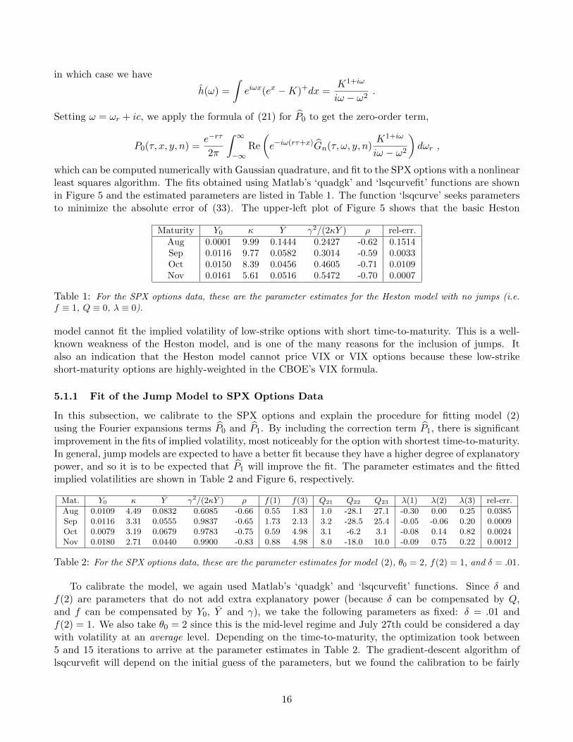
which can be computed numerically with Gaussian quadrature, and fit to the SPX options with a nonlinearleast squares algorithm. The fits obtained using Matlab’s ‘quadgk’ and ‘lsqcurvefit’ functions are shownin Figure 5 and the estimated parameters are listed in Table 1. The function ‘lsqcurve’ seeks parametersto minimize the absolute error of (33). The upper-left plot of Figure 5 shows that the basic Heston

Maturity Y0 κ Y γ2/(2κY ) ρ rel-err.Aug 0.0001 9.99 0.1444 0.2427 -0.62 0.1514Sep 0.0116 9.77 0.0582 0.3014 -0.59 0.0033Oct 0.0150 8.39 0.0456 0.4605 -0.71 0.0109Nov 0.0161 5.61 0.0516 0.5472 -0.70 0.0007

Table 1: For the SPX options data, these are the parameter estimates for the Heston model with no jumps (i.e.f ≡ 1, Q ≡ 0, λ ≡ 0).

model cannot fit the implied volatility of low-strike options with short time-to-maturity. This is a well-known weakness of the Heston model, and is one of the many reasons for the inclusion of jumps. Italso an indication that the Heston model cannot price VIX or VIX options because these low-strikeshort-maturity options are highly-weighted in the CBOE’s VIX formula.

5.1.1 Fit of the Jump Model to SPX Options Data

In this subsection, we calibrate to the SPX options and explain the procedure for fitting model (2)using the Fourier expansions terms P0 and P1. By including the correction term P1, there is significantimprovement in the fits of implied volatility, most noticeably for the option with shortest time-to-maturity.In general, jump models are expected to have a better fit because they have a higher degree of explanatorypower, and so it is to be expected that P1 will improve the fit. The parameter estimates and the fittedimplied volatilities are shown in Table 2 and Figure 6, respectively.

Mat. Y0 κ Y γ2/(2κY ) ρ f(1) f(3) Q21 Q22 Q23 λ(1) λ(2) λ(3) rel-err.

Aug 0.0109 4.49 0.0832 0.6085 -0.66 0.55 1.83 1.0 -28.1 27.1 -0.30 0.00 0.25 0.0385Sep 0.0116 3.31 0.0555 0.9837 -0.65 1.73 2.13 3.2 -28.5 25.4 -0.05 -0.06 0.20 0.0009Oct 0.0079 3.19 0.0679 0.9783 -0.75 0.59 4.98 3.1 -6.2 3.1 -0.08 0.14 0.82 0.0024Nov 0.0180 2.71 0.0440 0.9900 -0.83 0.88 4.98 8.0 -18.0 10.0 -0.09 0.75 0.22 0.0012

Table 2: For the SPX options data, these are the parameter estimates for model (2), θ0 = 2, f(2) = 1, and δ = .01.

To calibrate the model, we again used Matlab’s ‘quadgk’ and ‘lsqcurvefit’ functions. Since δ andf(2) are parameters that do not add extra explanatory power (because δ can be compensated by Q,and f can be compensated by Y0, Y and γ), we take the following parameters as fixed: δ = .01 andf(2) = 1. We also take θ0 = 2 since this is the mid-level regime and July 27th could be considered a daywith volatility at an average level. Depending on the time-to-maturity, the optimization took between5 and 15 iterations to arrive at the parameter estimates in Table 2. The gradient-descent algorithm oflsqcurvefit will depend on the initial guess of the parameters, but we found the calibration to be fairly

16

Figure 5: The implied volatilities of July 27th SPX options, alongside those of a fitted Heston model with no jumps(i.e. f ≡ 1, Q ≡ 0, and λ ≡ 0).

robust to this initial guess. Alternatively, one could look ahead to the parameter estimates in Table 3and use them as an initial guess.

5.2 Calibration of VIX Options

Calibration of model (2) to VIX options is much faster than calibrating to SPX options; it takes on theorder of 1 minute to generate the estimates and plots in Table 3 and Figure 7, respectively. Therefore, itmakes sense to first calibrate to VIX options, and then use these parameters to fit the SPX options, andthen re-adjust if needed. This section will explore the calibration of the model to the VIX options andmake comparisons of the VIX options’ parameters to those of the SPX options.

5.2.1 Numerical Computation of Y ’s Transition Density using Laguerre Polynomials

For α ≥ 0, let Zt be a square-root process such that

dZt = (1 + α− Zt)dt+√

2Zt dBt

where Bt is the same Brownian motion as in (2). The transition density for this process can be writtenin terms of an infinite series of Laguerre polynomials (see [21, 29]):

d

dz′P(Zt ≤ z′|Zt = z) = µα(z′)

∞∑`=0

Lα` (z′)Lα` (z)e−`(T−t) ∀t ≤ T and ∀z, z′ ∈ R+ ,

17

Figure 6: The implied volatilities of July 27th SPX options, alongside those of a fitted Heston model with jumps(i.e. λ 6= 0). Notice the improvement in the shortest time-to-maturity compared to the fit of the same option inFigure 5.

where µα(z) = zαe−z

Γ(α+1) , Lα` denotes the `th generalized Laguerre polynomial

Lα` (z) = ezz−(`+α) d`

dz`

(e−zz`+α

)( `! Γ(α+ 1)

Γ(`+ α+ 1)

)−1/2

, (35)

and Γ denotes the Gamma function. These polynomials form an orthonormal basis with respect to µα,∫Lα` (z)Lα`′(z)µ

α(z)dz = 1[`=`′] .

Furthermore, for α = 2κYγ2 − 1, it can be verified that

Ytd=γ2

2κZκt ,

and so the transition density in (32) can be well-approximated with the first 16 orthonormal polynomials,

d

dy′P(YT ≤ y′|Yt = y) =

d

dy′P(Zκ(T−t) ≤

2κ

γ2y′∣∣∣Z0 =

2κ

γ2y

)≈ 2κ

γ2µα(

2κ

γ2y′) 15∑`=0

Lα`

(2κ

γ2y′)Lα`

(2κ

γ2y

)e−`κ(T−t) . (36)

Taking 16 basis elements in (36) is equivalent to approximating the density with a 15-degree polynomial,which is a very good approximation provided that y is not far into the tail of Y ’s probability distribution.

18

The approximation in (36) is faster and more stable than a quadrature approximation of (32), and so wewill use this formula when calibrating to the VIX options data.

5.2.2 Fit of Jump Model to VIX Options Data

In calibrating model (2) to VIX options, the choice of parameters (f(1), f(3)) is crucial because theyimpact the volatility process σt = f(θt)

√Yt, allowing significant probability mass outside the range of

the typical square-root process. The implied volatility fits are shown in Figure 7 and the estimatedparameters in Table 3. From the figure it is clear that we have managed to price out-of-the-money VIX

mat. Y0 κ Y γ2/(2Y κ) f(1) f(3) Q21 Q22 Q23 λ(1) λ(2) λ(3) rel-err.

Aug 0.0180 8.19 0.0357 0.9894 1.0 3.0 15.1 -38.2 23.2 -0.060 0.041 0.037 0.1463Sep 0.0115 4.72 0.0454 0.9893 2.0 3.9 15.3 -27.7 12.4 -0.060 -0.000 0.098 0.0458Oct 0.0100 2.46 0.0832 0.9891 0.5 4.6 15.0 -22.4 7.4 -0.002 0.000 0.000 0.0108Nov 0.0100 1.86 0.0994 0.9871 0.6 4.7 15.0 -19.2 4.2 -0.007 -0.000 -0.004 0.0330

Table 3: For the VIX options data, these are the parameter estimates for model (2), θ0 = 2, δ = .01, f(2) = 1.

Figure 7: The implied volatilities of July 27th VIX options, alongside those of a fitted Heston with jumps. Thevertical line marks the VIX futures price on the date of maturity.

call options that were previously beyond the scope of the Heston model, and so we can conclude that theaddition of volatility regime-change has made a difference.

The parameters in Table 3 differ from those in Table 2, some by a small relative amount, some bymore, so it is hard to determine the degree of consistency between the two markets. However if we takethe VIX option-calibrated parameters and compute the model’s SPX option prices, then we see in Figure8 that there is a distinct and striking mismatch, particularly for options with shorter time-to-maturity.

19

Figure 8: The implied volatilities of July 27th SPX options, alongside those of a Heston with jumps calculatedusing the parameter estimates of Table 3 (i.e. the parameters estimated from the VIX options data –not the SPXdata).

To determine if there was a possible fit that matches both markets, we did a simultaneous calibrationand found the mismatch to remain (see Table 4 and Figure 9). A similar mismatch in prices is also foundindependently in [33], wherein several stochastic volatility models were tested and found to be misspecifiedwhen fit to both S&P 500 and VIX data, and also in [12] where it was found that the information contentof the SPX was not identical to that of the VIX.

Mat. Y0 κ Y γ2

2κYρ f(1) f(3) Q21 Q22 Q23 λ(1) λ(2) λ(3) rel-err.

SPX VIX.

Aug 0.03 8.58 0.0299 0.99 -0.67 0.82 3.02 14.6 -41.0 26.4 -0.01 0.04 0.09 0.06 0.16Sep 0.01 4.72 0.0452 0.99 -0.65 1.98 3.90 15.3 -27.7 12.4 -0.06 -0.00 0.10 0.03 0.13Oct 0.01 2.46 0.0813 0.99 -0.75 0.53 4.55 15.0 -22.4 7.3 -0.00 0.00 0.00 0.05 0.11Nov 0.01 1.86 0.0993 0.99 -0.84 0.60 4.74 15.3 -19.6 4.2 -0.00 -0.07 0.01 0.01 0.03

Table 4: A simultaneous fit to both the VIX and SPX options, θ0 = 2, f(2) = 1, and δ = .01. Both the relativeerror of the fit for SPX options and VIX options has increased from this reported in Tables 2 and 3, respectively.

20

Figure 9: The implied volatilities of July 27th SPX options (left column) and VIX options (right column), plottedalongside those of a fitted Heston with jumps. The vertical lines in the plots on the right mark the VIX futuresprice on the date of maturity.

21

It should be pointed out that we have only fit a narrow range of strikes for VIX call options. Aftercleaning the data of options that could be deemed illiquid because of low volume and/or little openinterest, we were left with roughly 12 options for each maturity, namely, those options with strike nearthe money and those with strikes 10 points higher. If we were to fit the extremely low and extremely highstrike options, we might find ourselves limited by only three regimes. Indeed, more regimes means morespreading-out of the probability mass, and thus might be effective in fitting all listed options. However,a model with too many regimes might be considered unfounded, as the clear explanation for using threedistinct regimes can have a certain amount of appeal in practice (e.g. for the VIX tail hedge).

5.2.3 Comparison of VIX Parameters: Crisis vs. Post-Crisis Era

In this section, we compare VIX options data from the crisis of Fall 2008 to data from a non-crisis period.In both cases we calibrate to the most liquid options with the shortest time-to-maturity. For the crisiswe consider the dates of October 8th through 16th of 2008. The VIX was at 57% on the 8th, and rose toa high of 80% on October 27th (and hit 80% again in November), and would not drop below 40% untilJanuary 2nd of 2009. For the non-crisis dates we consider February 4th through 14th of 2011, a periodin which there was little fear in the markets, as the VIX stayed down at roughly 15%.

The parameter estimates for October 2008 are shown in Table 5. Notice in these estimates that the

Day Y0 κ Y γ2/(2Y κ) f(1) f(3) Q31 Q32 Q33 λ(1) λ(2) λ(3) rel-err.8th 0.0100 2.56 0.0604 0.7338 0.5 3.1 0.7 -1.4 0.7 -0.001 -0.000 0.020 0.00249th 0.0100 3.02 0.0577 0.8679 0.5 3.6 3.2 -6.3 3.1 -0.000 0.000 0.020 0.013110th 0.0100 2.34 0.0571 0.8343 0.5 4.0 1.1 -2.2 1.1 -0.001 -0.000 0.020 0.002613th 0.0100 4.33 0.0716 0.7851 0.5 3.2 0.4 -0.8 0.4 -0.001 -0.000 0.020 0.113714th 0.0100 4.51 0.0581 0.4600 0.5 3.2 0.2 -0.4 0.2 -0.001 0.000 0.020 0.011315th 0.0100 3.81 0.0696 0.6603 0.5 3.6 0.2 -0.5 0.2 -0.001 0.000 0.020 0.002216th 0.0100 2.73 0.0942 0.6843 0.5 4.0 0.5 -1.0 0.5 -0.001 0.000 0.020 0.0070

Table 5: Parameter estimates for 2008 Crisis data. Calibration to VIX Options of October 2008, θ0 = 3, δ = .01,f(2) = 1.

regime is in the high state (θ0 = 3) and the risk-neutral probability of switching out is very low (Q33 ≈ −1so that P(regime change) ≈ 1 − e−1/365 ≈ .003). These parameters characterize the fear at that time,which was the belief that things were going to get a lot worse. Indeed, implied volatility of high-strikeVIX calls was not increasing during October 2008 because the VIX future was extremely high; the flatimplied volatility of high-strike VIX options during the crisis is seen in Figure 10.

The parameter estimates for February 2011 are shown in Table 6. In contrast to those in Table 5,

Day Y0 κ Y γ2/(2Y κ) f(1) f(3) Q21 Q22 Q23 λ(1) λ(2) λ(3) rel-err.4th 0.0150 3.98 0.0290 0.6577 0.5 3.9 1.0 -18.6 17.5 -0.001 0.000 0.168 0.50137th 0.0150 4.06 0.0232 0.6237 0.5 4.0 1.0 -18.0 17.0 -0.001 0.000 0.181 0.61598th 0.0150 4.06 0.0195 0.6201 0.5 4.0 1.0 -18.0 17.0 -0.001 0.000 0.184 0.60039th 0.0150 4.19 0.0209 0.5459 0.5 3.8 1.0 -17.9 16.9 -0.001 0.000 0.192 0.527010th 0.0150 4.09 0.0344 0.6153 0.5 4.0 1.0 -18.0 17.0 -0.001 0.000 0.150 1.260111th 0.0150 4.07 0.0332 0.6217 0.5 4.0 1.0 -18.0 17.0 -0.001 0.000 0.128 1.360414th 0.0150 4.17 0.0127 0.8813 0.5 3.9 1.0 -18.0 16.9 -0.001 0.000 -0.148 0.525515th 0.0150 4.23 0.0135 0.7905 0.5 3.9 1.0 -18.0 17.0 -0.002 0.000 0.187 0.8480

Table 6: Parameter Estimates for the Post-Crisis Data. Calibration to VIX Options of February 2011, θ0 = 2,δ = .01, f(2) = 1.

the regime is θ0 = 2 because there is certainly not a high-volatility state, but the probability of jumping

22

Figure 10: Top: Implied volatilities of VIX options during the Crisis of October 2008, fitted with the parametersof Table 5. The vertical is the VIX futures price; the belief during the crisis was that things were going to get a lotworse, so the VIX future was very high, and high-strike VIX options had low implied volatility.

to the high state looms as Q22 ≈ −18 (the risk-neutral probability of a jump is significantly higher thanbefore as P(regime change) ≈ 1−e−18/365 ≈ .05). Historically, February 2011 was a relatively calm periodfor the VIX (and the SPX), but high-strike VIX options are somewhat of an insurance contract againstoutlier events, and so they trade at a premium for the same reason that low-strike SPX put options tradeat a premium. The implied volatilities of these VIX options are shown in Figure 11, where we see anincrease in implied volatility for high strikes caused by the probability of jumping to the high-volatilityregime, aka by crash-o-phobia.

Finally, we should make a few remarks on the sensitivity of the parameter estimation procedure. Itwas mentioned in Section 5.1.1 that calibration of the model in (2) is a non-convex optimization, and it iswell-known that non-convex problems are sensitive to the initial guess that is input to the optimizationalgorithm. Hence, we see in Tables 5 and 6 that parameters associated with states that have littleprobability of occurring will not change much from their initial guess, as these parameters have littlebearing on the fit (that is why we only fit Qθ01, Qθ02, and Qθ03).

6 Conclusion

Motivated by the frequent observation that the Heston stochastic volatility model cannot fit the impliedvolatiles of VIX options, we analyzed and implemented an extension which incorporates regime switchingand jumps. Using asymptotic expansions of the Fourier transforms, we can efficiently price SPX andVIX options. When applied to market data, the model captures the implied volatility skews of both

23

Figure 11: Top: Implied volatilities of VIX options during February 2011, fitted with the parameters of Table 6.

the SPX and VIX separately, but highlights a distinct discrepancy between the two markets. We alsocalibrated the model to VIX options from the 2008 financial crisis and to non-crisis data of 2011, andwere able to relate the parameter estimates to the historical beliefs about volatility fears during theseperiods, confirming the importance of regime switches.

Acknowledgements

The authors thank Lisa Goldberg for discussion on regime models, as well as Jim Gatheral and twoanonymous referees for their helpful comments.

References

[1] Y. Ait-Sahalia, M. Karaman, and L. Mancini. The term structure of variance swaps, risk premia and the ex-pectation hypothesis. Working paper, Princeton University, 2012. Available at http://ssrn.com/abstract=2136820.

[2] G. Bakshi, C. Cao, and Z. Chen. Empirical performance of alternative option pricing models. The Journal ofFinance, 52(5):2003–2049, 1997.

[3] J. Baldeaux and A. Badran. Consistent modeling of VIX and equity derivatives using a 3/2 plus jumps model.Research Paper Series 306, Quantitative Finance Research Centre, University of Technology, Sydney, March2012. Available at http://ideas.repec.org/p/uts/rpaper/306.html.

[4] C. Bayer, J. Gatheral, and M. Karlsmark. Fast Ninomiya-Victoir calibration of the double-mean-revertingmodel. 2013. Available at http://papers.ssrn.com/sol3/papers.cfm?abstract_id=2210420.

24

[5] T. Bollerslev and V. Todorov. Tails, fears, and risk premia. Journal of Finance, 66(6):2165–2211, December2011.

[6] P. Carr and R. Lee. Volatility derivatives. Annual Review of Financial Economics, 1:319–339, 2009.

[7] P. Carr and D. Madan. Towards a theory of volatility trading. In M. Musiella, E. Jouini, and J. Cvitanic,editors, Option Pricing, Interest Rates, and Risk Management, pages 417–427. University Press, 1998.

[8] P. Carr, D. Madan, and R. Smith. Option valuation using the fast Fourier transform. Journal of ComputationalFinance, 2:61–73, 1999.

[9] P. Carr and L. Wu. Variance risk premiums. The Review of Financial Studies, 22:1311–1341, March 2009.

[10] L. Chan, R.J. Elliot, and T.K. Siu. Pricing volatility swaps under heston’s stochastic volatility model withregime change. Applied Mathematical Finance, 14(1):41–62, 2007.

[11] L. Chan, R. J. Elliott, J.W. Lau, and T.K. Siu. Pricing options under a generalized Markov-modulatedjump-diffusion model. Stochastic Analysis and Applications, 25(4):821–843, 2007.

[12] S. Chung, W. Tsai, Y. Wang, and P. Weng. The information content of the S&P 500 index and VIX optionson the dynamics of the S&P 500 index. Journal of Futures Markets, 31(12):1170–1201, 2011.

[13] R. Cont and T. Kokholm. A consistent pricing model for index options and volatility derivatives. MathematicalFinance, 23(2):248–274, 2013.

[14] R. Daigler and Z. Wang. The performance of VIX option pricing models: Empirical evidence beyond simulation.The Journal of Futures Markets, 31(3):251281, 2011.

[15] G. Drimus. Options on realized variance by transform methods: a non-affine stochastic volatility model.Quantitative Finance, 2012. forthcoming.

[16] J. Duan and C. Yeh. Jump and volatility risk premiums implied by VIX. Journal of Economic Dynamics andControl, 34(11):2232–2244, November 2010.

[17] D. Duffie, D. Filipovic, and W. Schachermayer. Affine processes and applications in finance. Annals of AppliedProbability, 13:984–1053, 2003.

[18] D. Duffie, J. Pan, and K. Singleton. Transform analysis and asset pricing for affine jump-diffusions. Econo-metrica, 68:1343–1376, 2000.

[19] B. Eraker. Do stock prices and volatility jump? Reconciling evidence from spot and options prices. TheJournal of Finance, 59(3):1367–1404, 2004.

[20] J.P. Fouque and M. Lorig. A fast mean-reverting correction to Heston’s stochastic volatility model. SIAMJournal on Financial Mathematics, 2:221–254, 2011.

[21] J.P. Fouque, G. Papanicolaou, R. Sircar, and K. Sølna. Multiscale Stochastic Volatility for Equity, InterestRate, and Credit Derivatives. Cambridge University Press, 2011.

[22] J. Gatheral. The Volatility Surface: A Practitioner’s Guide. Wiley, 2006.

[23] J. Gatheral. Consistent modeling of SPX and VIX options. Presented at The Fifth World Congress of theBachelier Finance Society in London, 2008. Available at: http://www.math.nyu.edu/fellows_fin_math/

gatheral/Bachelier2008.pdf.

[24] J. Hamilton. Regime switching models. In S. Durlauf and L. Blume, editors, The New Palgrave Dictionary ofEconomics. Palgrave Macmillan, 2nd edition, 2008.

[25] S. Heston. A closed-form solution for options with stochastic volatility with applications to bond and currencyoptions. Review of Financial Studies, 6:327–343, 1993.

[26] E. Hillebrand. Neglecting parameter changes in GARCH models. Journal of Econometrics, 129(1-2):121–138,2005.

[27] S. Howison, A. Rafailidis, and H. Rasmussen. On the pricing and hedging of volatility derivatives. AppliedMathematical Finance, 11(4):317–346, 2004.

25

[28] A. L. Lewis. Option Valuation under Stochastic Volatility with Mathematica Code. Finance Press, 2000.

[29] V. Linetsky. Spectral methods in derivative pricing. In Handbooks in Operations Research and ManagementScience: Financial Engineering, volume 15, chapter 6, pages 223–299. Elsevier B.V., 2007.

[30] D. Madan and M. Yor. The S&P 500 index as a Sato process travelling at the speed of the VIX. AppliedMathematical Finance, 18(3):227–244, 2011.

[31] J. Mencıa and E. Sentana. Valuation of VIX derivatives. Working Papers wp2009 0913, CEMFI, December2009. Available at: http://ideas.repec.org/p/cmf/wpaper/wp2009_0913.html.

[32] A. Sepp. Pricing options on realized variance in the Heston model with jumps in returns and volatility. Journalof Computational Finance, 11(4):33–70, 2008.

[33] Z. Song and D. Xiu. A tale of two option markets: State-price densities implied from S&P 500 and VIXoption prices. Working paper, Chicago Booth, 2012. Available at http://papers.ssrn.com/sol3/papers.

cfm?abstract_id=2013381.

[34] G. Tauchen and V. Todorov. Volatility jumps. Journal of Business and Economic Statistics, 29:356–371, 2011.

26