Embed Size (px)
Citation preview
A Reduced Three Dimensional Dynamic
Structural Model for Structural Health
Assessment
Luther WhiteDepartment of Mathematics
University of OklahomaNorman, Oklahoma 73019
April 19, 2006
Abstract
Dynamic models of elastic structures are derived using approximationsof linear three dimensional elasticity. A model for the three dimensionalmotion of a nonsymmetric structure that is of use for applications tohealth monitoring for buildings is obtained. The symmetric version ofthe model is validated using laboratory acceleration data. Narrow plateequations whose derivation is based on similar consideration but with platethinness assumptions are used in a probabilistic inversion for elastic andmass properties from acceleration data. Finally, predictions of structuralbehavior based on the information from the inversion problem are made.
1. Introduction.
We derive three dimensional dynamic models for structures. The derivation isanalogous to that of the so-called narrow plate models of intermediate natu-ral between beams and plates. In [7, 8, 9] narrow plate models are presented.Also, narrow plate models are validated against spectral data and static modelsare studied. In the current work, however, dynamic time dependent modelsare presented and derived without the thickness assumption imposed on plates[2,4,7,8,9]. Displacement approximations are assumed that are similar to thosefor narrow plates and generalizations of Timoshenko beam models [1]. How-ever, they are specializations of the Mindlin plate model [4]. The objective ofour modelling effort is to obtain a three dimensional model that is suitable forassessment of the structural health of buildings. Our model allows for nonsym-metric properties in the structure. However, at this early stage of developmentwe present the model, but compare only to laboratory structures that are sym-
1
metric. A numerical inversion of acceleration data is presented as well as pre-dictions of likely structural responses based on a posteriori probability densityfunctions.
In Section 2 we present the derivation of the equations that include basemotion. The derivations are based on the small displacement gradient assump-tion of linear elasticity [2]. Geometric symmetry of the structure about a centralaxis is assumed. However, in order to accommodate possible structural damage,material properties are not assumed symmetric. The spatially discrete time de-pendent model is presented that includes a moving base. In Section 3 we presenta specialization of our model to the classical Euler-Bernoulli beam with a tipmass to illustrate a comparison between our model and the tip mass model. InSection 4 we compare our computed accelerations with those observed in thelaboratory. We find that our results qualitatively support this application ofthe model. In Section 5 we formulate a inverse problem using acceleration datato provide probabilistic estimates of material parameters. These estimates arethen used to make predictions of likely behavior of the structure under a givenforce.
2. The underlying model equations.
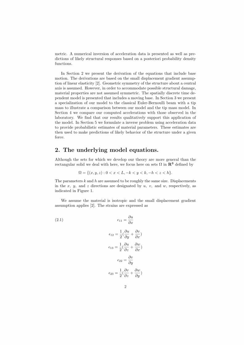
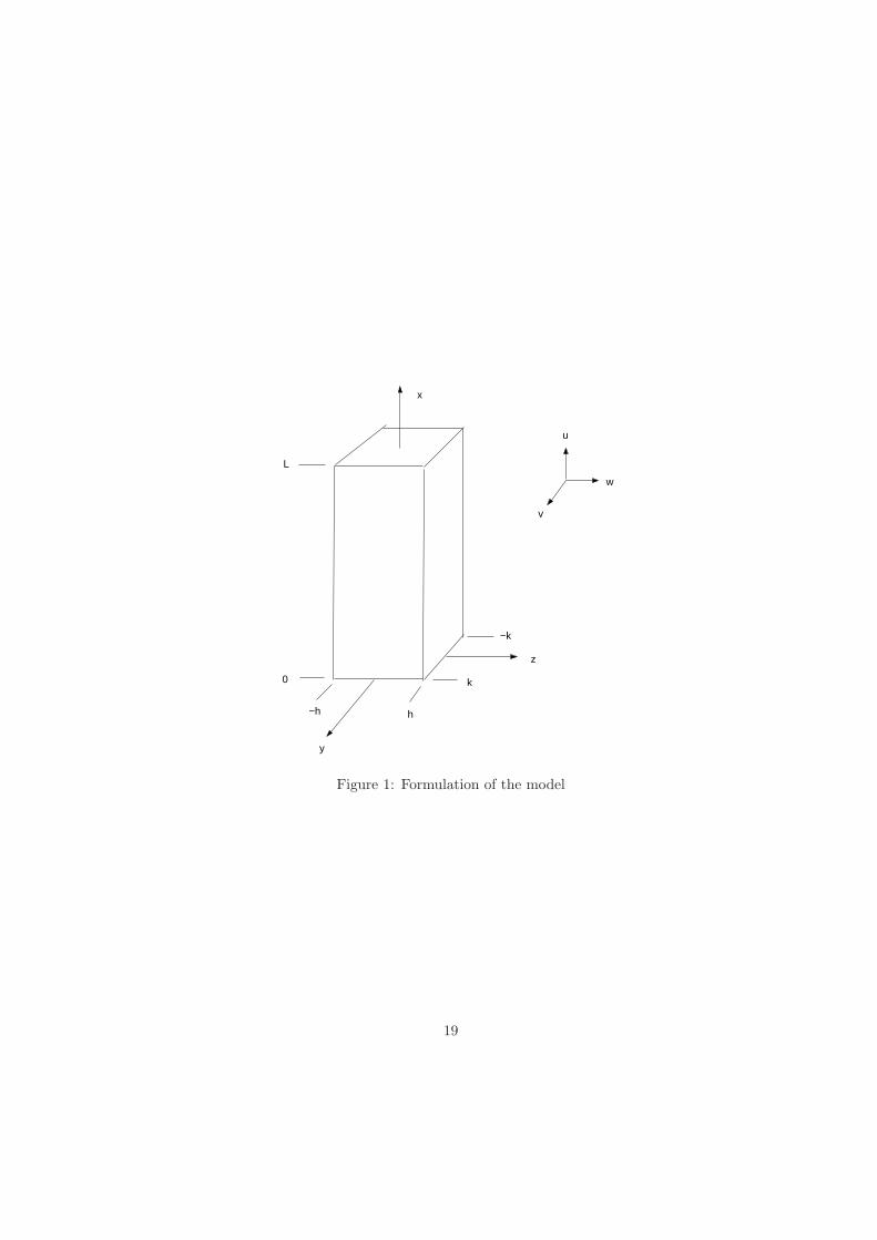
Although the sets for which we develop our theory are more general than therectangular solid we deal with here, we focus here on sets Ω in R3 defined by
Ω = (x, y, z) : 0 < x < L,−k < y < k,−h < z < h.The parameters k and h are assumed to be roughly the same size. Displacementsin the x, y, and z directions are designated by u, v, and w, respectively, asindicated in Figure 1.
We assume the material is isotropic and the small displacement gradientassumption applies [2]. The strains are expressed as
(2.1) ε11 =∂u
∂x
ε12 =12(∂u
∂y+
∂v
∂x)
ε13 =12(∂u
∂z+
∂w
∂x)
ε22 =∂v
∂y
ε23 =12(∂v
∂z+
∂w
∂y)
2

ε33 =∂w
∂z.
The stresses are expressed as
(2.2) σ11 =E
(1 + µ)(1− 2µ)[(1− µ)ε11 + µε22 + µε33]
σ12 =2E
1 + µε12
σ13 =2E
1 + µε13
σ22 =E
(1 + µ)(1− 2µ)[µε11 + (1− µ)ε22 + µε33]
σ23 =2E
1 + µε23
σ33 =E
(1 + µ)(1− 2µ)[µε11 + µε22 + (1− µ)ε33]
where E is Young’s modulus and µ is Poisson’s ratio. We do not impose geo-metric assumptions on the stresses at this point as is done with beam and platemodels. Nevertheless, displacements are constrained under an assumption thatthe length dimensions in the y and z dimensions are roughly the same order.The displacement functions are expanded as truncated series in y and z withcoefficients as functions of x. Towards this end displacement functions
(2.3) u(x, y, z) = u0(x) + zu1(x) + yu2(x) + yzu3(x)
v(x, y, z) = v0(x) + zv1(x) + z2v2(x)
w(x, y, z) = w0(x) + yw1(x) + y2w2(x).
These expressions amount to approximation in the y and z variables in a phys-ically meaningful way. The stress-free boundary conditions on the lateral facesare variational boundary conditions and, hence, are not imposed on the approx-imating elements. It follows that the corresponding strains are given by
(2.4) ε11 = u0x + zu1x + yu2x + yzu3x
ε12 =12u2 + v0x + z(u3 + v1x) + z2v2x
ε13 =12u1 + w0x + y(u3 + w2x) + y2w2x
3
ε22 = 0
ε23 =12v1 + w1 + 2zv2 + 2yw2
ε33 = 0.
The stresses are expressed as
(2.5) σ11 =(1− µ)E
(1 + µ)(1− 2µ)[u0x + zu1x + yu2x + yzu3x]
σ12 =2E
1 + µ[u2 + v0x + z(u3 + v1x) + z2v2x]
σ13 =2E
1 + µ[u1 + w0x + y(u3 + w1x) + y2w2x]
σ22 =µE
(1 + µ)(1− 2µ)[u0x + zu1x + yu2x + yzu3x]
σ23 =2E
1 + µ[v1 + w1 + 2zv2 + 2yw2]
σ33 =µE
(1 + µ)(1− 2µ)[u0x + zu1x + yu2x + yzu3x].
The energy due to strain is expressed as
(2.6) V =12
∫
Ω
σ11ε11 + 2σ12ε12+
+2σ13ε13 + σ22ε22 + 2σ23ε23 + σ22ε22dzdydx
Substituting relations from (2.4) and (2.5) into (2.6), we obtain
(2.7) V =12
∫
Ω
(1− µ)E(1 + µ)(1− 2µ)
[u0x + zu1x + yu2x + yzu3x]2
+2E
1 + µ[u2 + v0x + z(u3 + v1x) + z2v2x]2+
+2E
1 + µ[u1 + w0x + y(u3 + w1x) + y2w2x]2+
+2E
1 + µ[v1 + w1 + 2zv2 + 2yw2]2dzdydx.
4
The Young’s modulus E and Poisson’s ratio µ are taken to be dependent on thespatial variables. In general no symmetry in the functions E and µ is assumed;hence,
E = E(x, y, z)
andµ = µ(x, y, z).
Define the following matrix-valued functions of x.
(2.8)
k0(x) =∫ k
−k
∫ h
−h
(1− µ(x, y, z))E(x, y, z)(1 + µ(x, y, z))(1− 2µ(x, y, z))
1 z y yzz z2 yz yz2
y yz y2 y2zyz yz2 y2z y2z2
dzdy
(2.9) a0(x) =∫ k
−k
∫ h
−h
2E(x, y, z)1 + µ(x, y, z)
1 z z2
z z2 z3
z2 z3 z4
dzdy
(2.10) b0(x) =∫ k
−k
∫ h
−h
2E(x, y, z)1 + µ(x, y, z)
1 y y2
y y2 y3
y2 y3 y4
dzdy
(2.11) c0(x) =∫ k
−k
∫ h
−h
2E(x, y, z)1 + µ(x, y, z)
1 2z 2y2z 4z2 4zy2y 4zy 4y2
dzdy.
With these assignments the strain potential energy takes the form
(2.12) V =12
∫ L
0
[u0 u1 u2 u3]x k0(x)
u0
u1
u2
u3
x
+
+[u2 + v0x u3 + v1x v2x] a0(x)
u2 + v0x
u3 + v1x
v2x
+
+[u1 + w0x u3 + w1x w2x] b0(x)
u1 + w0x
u3 + w1x
w2x
+
+[v1 + w1 v2 w2]c0(x)
v1 + w1
v2
w2
dx.
5

Define the vector-valued function x 7→ V(x) from R 7→ R10
V(x) = [u0(x) u1(x) u2(x) u3(x) v0(x) v1(x) v2(x) w0(x) w1(x) w2(x)]T
where T designates vector transpose. We write the strain energy explicitly interms of V by introducing the following matrices
Pu =
1 0 0 0 0 0 0 0 0 00 1 0 0 0 0 0 0 0 00 0 1 0 0 0 0 0 0 00 0 0 1 0 0 0 0 0 0
Pv =
0 0 0 0 1 0 0 0 0 00 0 0 0 0 1 0 0 0 00 0 0 0 0 0 1 0 0 0
Pw =
0 0 0 0 0 0 0 1 0 00 0 0 0 0 0 0 0 1 00 0 0 0 0 0 0 0 0 1
P1 =
0 1 0 0 0 0 0 0 0 00 0 0 1 0 0 0 0 0 00 0 0 0 0 0 0 0 0 0
P2 =
0 0 1 0 0 0 0 0 0 00 0 0 1 0 0 0 0 0 00 0 0 0 0 0 0 0 0 0
P3 =
0 0 0 0 0 1 0 0 1 00 0 0 0 0 0 1 0 0 00 0 0 0 0 0 0 0 0 1
.
With these assignments, the strain energy functional may be written as
(2.13) V =12
∫ L
0
VTx PT
u k0(x)PuVx + [P2V + PvVx]T a0(x)[P2V + PvVx]+
+[P1V + PwVx]T b0(x)[P1V + PwVx] + VT PT3 c0(x)P3Vdx.
Finally, for convenience define the matrices
(2.14) k(x) = PTu k0(x)Pu + PT
v a0(x)Pv + PTw b0(x)Pw
(2.14) a(x) = PTu a0(x)P2 + PT
w b0(x)P1
(2.15) b(x) = PT2 a0(x)P2 + PT
1 b0(x)P1 + PT3 c0(x)P3
6
and express the strain energy as
(2.16) V =12
∫ L
0
VTx k(x)Vx + VT
x a(x)V + VT a(x)T Vx + VT b(x)Vdx.
To introduce dynamics, we assume that the functions u, v, and w are de-pendent also on time t so that V = V(x, t). Introducing the density function(x, y, z) 7→ ρ(x, y, z) defined on Ω, the kinetic energy quadratic functional isgiven as
(2.17) K =12
∫
Ω
ρ(x, y, z)[u2t + v2
t + w2t ]dzdydx
where the displacement functions are considered to be dependent on time aswell as space. Substituting the expressions from (2.3) for u, v, and w, we have
K =12
∫
Ω
ρ(x, y, z)[u0t + zu1t + yu2t + yzu3t]2+
(2.18) +[v0t + zv1t + z2v2t]2 + [w0t + zw1t + z2w2t]2dzdydx.
Introducing the matrix(2.19)
m(x) =∫ k
−k
∫ h
−h
ρ(x, y, z)
1 z y yz 0 0 0 0 0 0z z2 yz yz2 0 0 0 0 0 0y yz y2 y2z 0 0 0 0 0 0yz yz2 y2z y2z2 0 0 0 0 0 00 0 0 0 1 z z2 0 0 00 0 0 0 z z2 z3 0 0 00 0 0 0 z2 z3 z4 0 0 00 0 0 0 0 0 0 1 y y2
0 0 0 0 0 0 0 y y2 y3
0 0 0 0 0 0 0 y2 y3 y4
dzdy,
the expression for kinetic energy can be written as
(2.20) T =12
∫ L
0
Vt(x, t)T m(x)Vt(x, t)dx.
The work done by external forces is expressed as
(2.21) W =∫ L
0
f(x, t)T V(x, t)dx.
Forming the Lagrangian and applying Hamilton’s principle [5] yields an initialboundary value problem. Finally, including a damping term for energy dissipa-tion, we obtain
7
(2.22) mVtt + cVt − (kVx + aV)x + aT Vx + bV = f
with initial conditions
(2.23) V(·, 0) = V0
V(·, 0) = V1
and boundary conditions that must satisfy
δV(kVx + aV)|L0 = 0.
Under boundary conditions that are clamped at x = 0 and free at x = L,we have
(2.24) V(0, t) = 0
and
(2.25) (kVx + aV)(L, t) = 0.
For many applications we want to include the possibility of a moving base.Thus, we wish to have a boundary condition
V(0, t) = W(t)
To adjust our model, we define a new function
(2.26) U(x, t) = V(x, t)−W(t)
and substitute into the differential equation. Carrying out this procedure, weobtain the equation
(2.27) mUtt + cUt − (kUx + aU)x + aT Ux + bU =
= f− [mWtt + cWt − (aW)x + bW]
with boundary conditions
(2.28) U(0, t) = 0
(2.29) [kUx + aU](L, t) = −aW(t).
Semidiscrete spatial approximations may be obtained using piecewise linearelements defined on a nonuniform mesh on (0, L), [6]. Let the interval (0, L) be
8
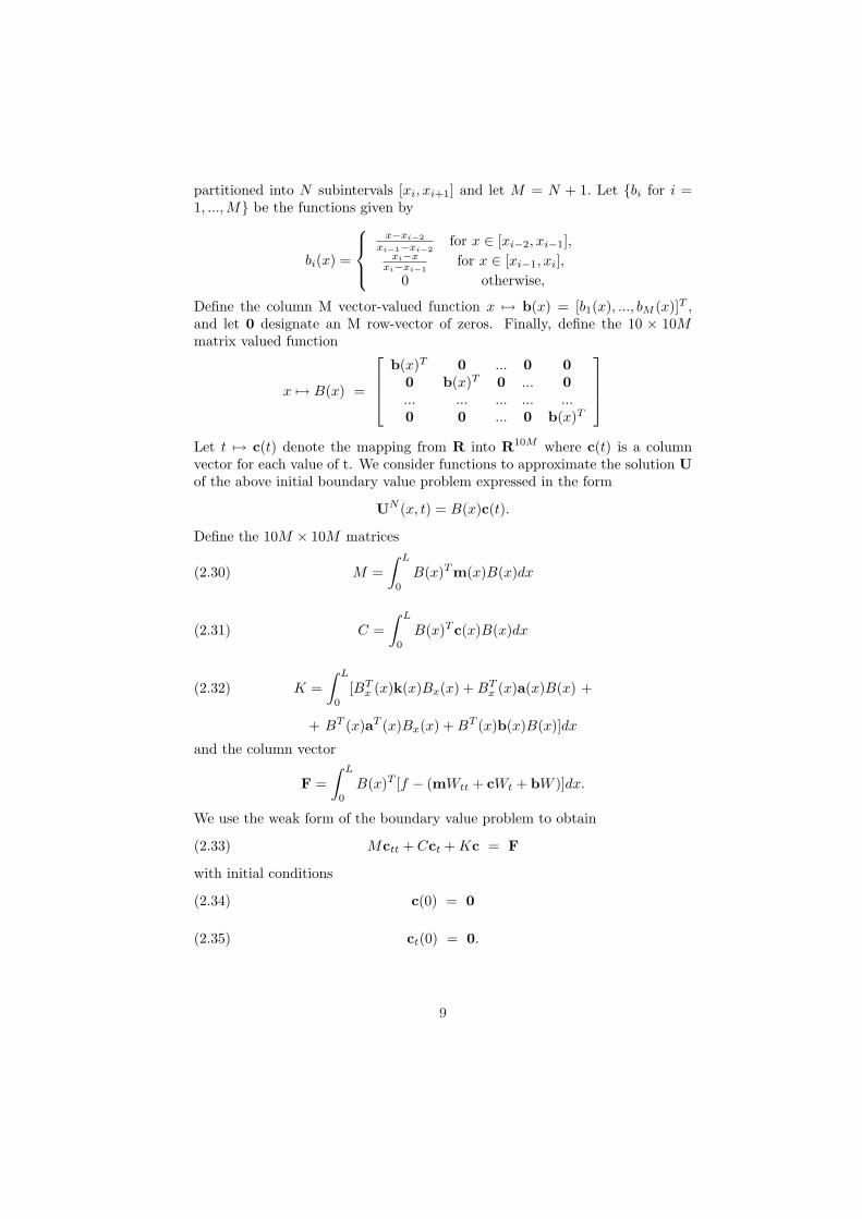
partitioned into N subintervals [xi, xi+1] and let M = N + 1. Let bi for i =1, ..., M be the functions given by
bi(x) =
x−xi−2xi−1−xi−2
for x ∈ [xi−2, xi−1],xi−x
xi−xi−1for x ∈ [xi−1, xi],
0 otherwise,
Define the column M vector-valued function x 7→ b(x) = [b1(x), ..., bM (x)]T ,and let 0 designate an M row-vector of zeros. Finally, define the 10 × 10Mmatrix valued function
x 7→ B(x) =
b(x)T 0 ... 0 00 b(x)T 0 ... 0... ... ... ... ...0 0 ... 0 b(x)T
Let t 7→ c(t) denote the mapping from R into R10M where c(t) is a columnvector for each value of t. We consider functions to approximate the solution Uof the above initial boundary value problem expressed in the form
UN (x, t) = B(x)c(t).
Define the 10M × 10M matrices
(2.30) M =∫ L
0
B(x)T m(x)B(x)dx
(2.31) C =∫ L
0
B(x)T c(x)B(x)dx
(2.32) K =∫ L
0
[BTx (x)k(x)Bx(x) + BT
x (x)a(x)B(x) +
+ BT (x)aT (x)Bx(x) + BT (x)b(x)B(x)]dx
and the column vector
F =∫ L
0
B(x)T [f − (mWtt + cWt + bW )]dx.
We use the weak form of the boundary value problem to obtain
(2.33) Mctt + Cct + Kc = F
with initial conditions
(2.34) c(0) = 0
(2.35) ct(0) = 0.
9
3. Comparison of model with simple Euler-Bernoulliwith tip-mass.
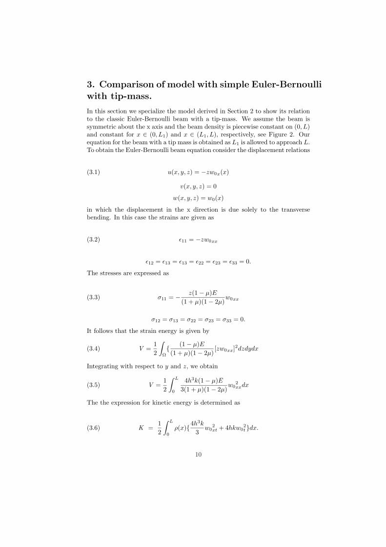
In this section we specialize the model derived in Section 2 to show its relationto the classic Euler-Bernoulli beam with a tip-mass. We assume the beam issymmetric about the x axis and the beam density is piecewise constant on (0, L)and constant for x ∈ (0, L1) and x ∈ (L1, L), respectively, see Figure 2. Ourequation for the beam with a tip mass is obtained as L1 is allowed to approach L.To obtain the Euler-Bernoulli beam equation consider the displacement relations
(3.1) u(x, y, z) = −zw0x(x)
v(x, y, z) = 0
w(x, y, z) = w0(x)
in which the displacement in the x direction is due solely to the transversebending. In this case the strains are given as
(3.2) ε11 = −zw0xx
ε12 = ε13 = ε13 = ε22 = ε23 = ε33 = 0.
The stresses are expressed as
(3.3) σ11 = − z(1− µ)E(1 + µ)(1− 2µ)
w0xx
σ12 = σ13 = σ22 = σ23 = σ33 = 0.
It follows that the strain energy is given by
(3.4) V =12
∫
Ω
(1− µ)E(1 + µ)(1− 2µ)
[zw0xx]2dzdydx
Integrating with respect to y and z, we obtain
(3.5) V =12
∫ L
0
4h3k(1− µ)E3(1 + µ)(1− 2µ)
w02xxdx
The the expression for kinetic energy is determined as
(3.6) K =12
∫ L
0
ρ(x)4h3k
3w0
2xt + 4hkw0
2tdx.
10
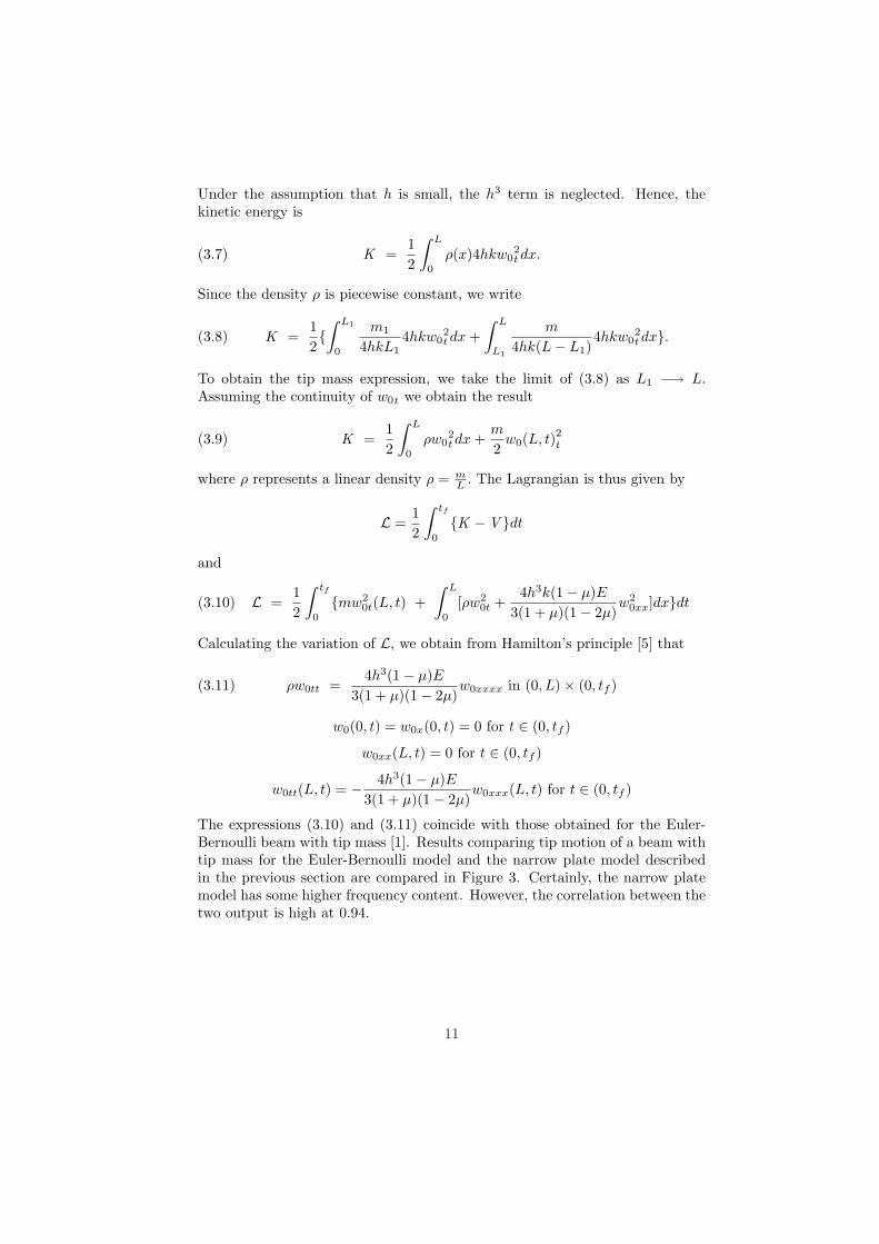
Under the assumption that h is small, the h3 term is neglected. Hence, thekinetic energy is
(3.7) K =12
∫ L
0
ρ(x)4hkw02t dx.
Since the density ρ is piecewise constant, we write
(3.8) K =12∫ L1
0
m1
4hkL14hkw0
2t dx +
∫ L
L1
m
4hk(L− L1)4hkw0
2t dx.
To obtain the tip mass expression, we take the limit of (3.8) as L1 −→ L.Assuming the continuity of w0t we obtain the result
(3.9) K =12
∫ L
0
ρw02t dx +
m
2w0(L, t)2t
where ρ represents a linear density ρ = mL . The Lagrangian is thus given by
L =12
∫ tf
0
K −V dt
and
(3.10) L =12
∫ tf
0
mw20t(L, t) +
∫ L
0
[ρw20t +
4h3k(1− µ)E3(1 + µ)(1− 2µ)
w20xx]dxdt
Calculating the variation of L, we obtain from Hamilton’s principle [5] that
(3.11) ρw0tt =4h3(1− µ)E
3(1 + µ)(1− 2µ)w0xxxx in (0, L)× (0, tf )
w0(0, t) = w0x(0, t) = 0 for t ∈ (0, tf )
w0xx(L, t) = 0 for t ∈ (0, tf )
w0tt(L, t) = − 4h3(1− µ)E3(1 + µ)(1− 2µ)
w0xxx(L, t) for t ∈ (0, tf )
The expressions (3.10) and (3.11) coincide with those obtained for the Euler-Bernoulli beam with tip mass [1]. Results comparing tip motion of a beam withtip mass for the Euler-Bernoulli model and the narrow plate model describedin the previous section are compared in Figure 3. Certainly, the narrow platemodel has some higher frequency content. However, the correlation between thetwo output is high at 0.94.
11
4. The comparison of model output with labora-tory data.
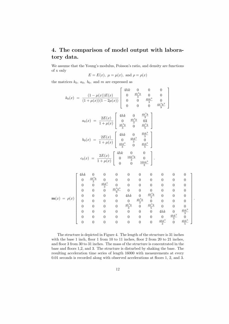
We assume that the Young’s modulus, Poisson’s ratio, and density are functionsof x only
E = E(x), µ = µ(x), and ρ = ρ(x)
the matrices k0, a0, b0, and m are expressed as
k0(x) =(1− µ(x))E(x)
(1 + µ(x))(1− 2µ(x))
4hk 0 0 00 4h3k
3 0 00 0 4hk3
3 00 0 0 4h3k3
9
a0(x) =2E(x)
1 + µ(x)
4hk 0 4h3k3
0 4h3k3 03
4h3k3 0 4h5k
5
b0(x) =2E(x)
1 + µ(x)
4hk 0 4hk3
3
0 4hk3
3 04hk3
3 0 4hk5
5
c0(x) =2E(x)
1 + µ(x)
4hk 0 00 16h3k
3 00 0 16hk3
3
.
m(x) = ρ(x)
4hk 0 0 0 0 0 0 0 0 00 4h3k
3 0 0 0 0 0 0 0 00 0 4hk3
3 0 0 0 0 0 0 00 0 0 4h3k3
9 0 0 0 0 0 00 0 0 0 4hk 0 4h3k
3 0 0 00 0 0 0 0 4h3k
3 0 0 0 00 0 0 0 4h3k
3 0 4h5k5 0 0 0
0 0 0 0 0 0 0 4hk 0 4hk3
3
0 0 0 0 0 0 0 0 4hk3
3 00 0 0 0 0 0 0 4hk3
3 0 4hk5
5
.
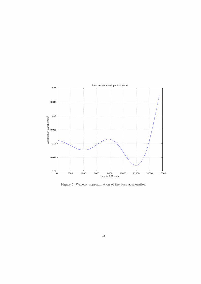
The structure is depicted in Figure 4. The length of the structure is 31 incheswith the base 1 inch, floor 1 from 10 to 11 inches, floor 2 from 20 to 21 inches,and floor 3 from 30 to 31 inches. The mass of the structure is concentrated in thebase and floors 1,2, and 3. The structure is disturbed by shaking the base. Theresulting acceleration time series of length 16000 with measurements at every0.01 seconds is recorded along with observed accelerations at floors 1, 2, and 3.
12
We thus set the force vector f to zero and obtain the associated base velocity anddisplacement vector functions by integrating the acceleration record. In fact weuse a Daubechy level 12 wavelet approximation to smooth the acceleration timeseries [3]. Base motion is portrayed in Figure 5. To approximate the equation,we use a finite element basis of piecewise linear functions described previouslybased on nodal locations
[0 1 4 7 10 11 14 17 20 21 24 27 30 31].
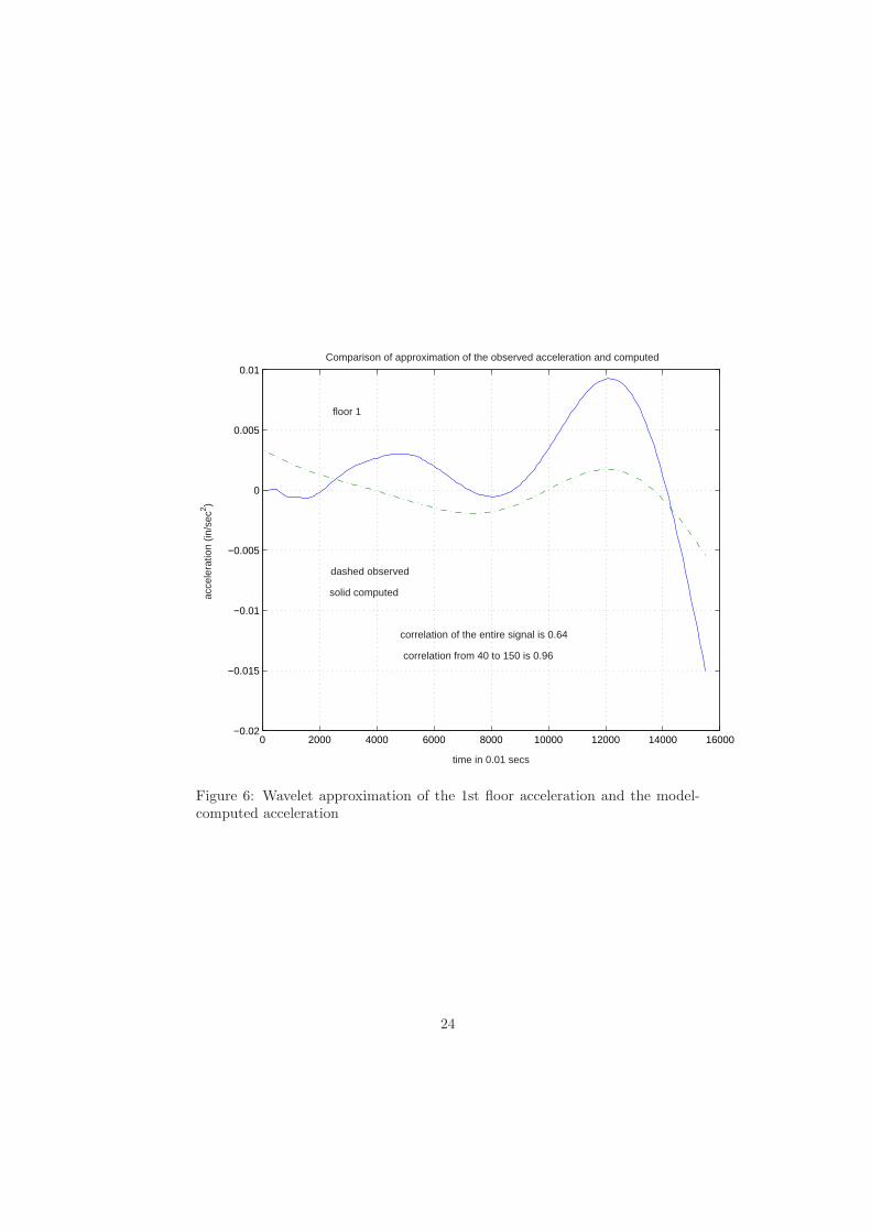
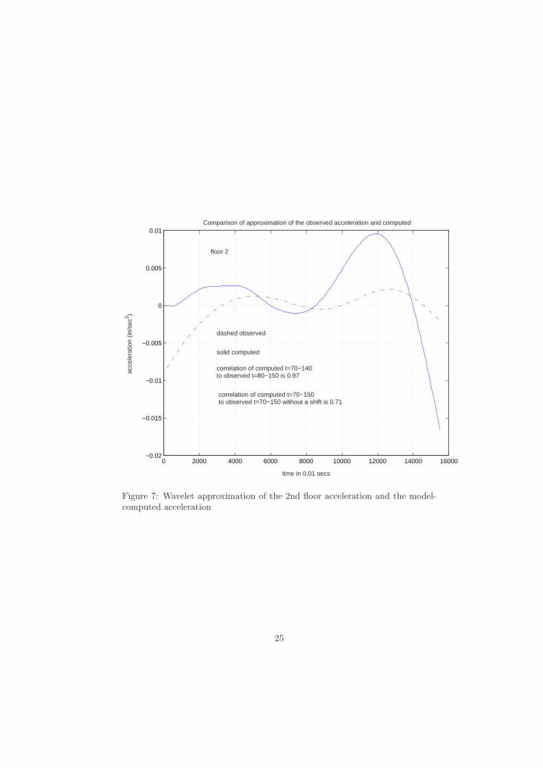
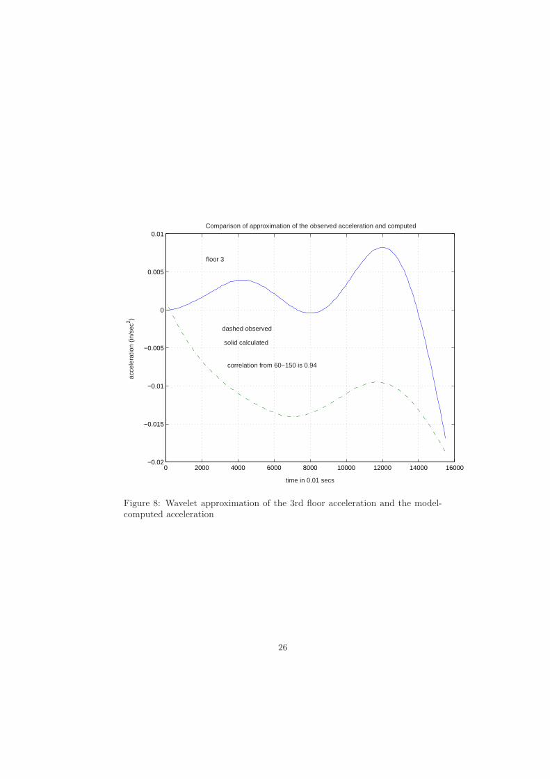
At this point we are interested primarily in the qualitative behavior of ourmodel. Hence, we set µ = 0. The only modelling of Young’s modulus and densityis that values of these parameters in intervals corresponding to the floors is verylarge as compared with those intervals associated with regions between floors. Asmall constant viscous damping term is also included. The initial value problemis solved numerically using a 1 sec time step and compared with the Daubechy12 wavelet approximation of the observed acceleration time series over a timeperiod of 155 seconds. The results are portrayed in Figures 6, 7, and 8. We notethat there is high correlation between signals over subintervals of the record inwhich initial effects are not included. For the second floor a comparison of ashifted records results in very high correlation of 0.97 compared to the 0.71correlation without shifting. For these examples this seems to be qualitativeevidence of a valid model.
5. Inversion of acceleration data.
In this section we use acceleration data to estimate material properties of astructure. We consider a slightly different set of displacement relations.
u(x, y, z, t) = u0(x, t) + zu1(x, t) + yzu2(x, t)
v(x, y, z, t) = v0(x, t) + zv1(x, t) + yzv2(x, t)
w(x, y, z, t) = w0(x, t) + yw1(x, t) + y2w2(x, t).
The model that we consider, a narrow ”bowed” plate, that is derived with theabove displacement relations and makes the plate thickness assumption thatnormal forces on the surface may be view as body forces. The stress σ33 is set tozero, and the resulting relation is used to solve for ε33 it terms of ε11 and ε22, see[7,8,9]. A system of initial boundary value problems analogous to those obtainedin Section 2 are obtained by means of a similar procedure. In this case we have asystem of nine partial differential equations with a single spatial variable. Thesolution is a column 9-vector V (x, t) = [u0, u1, u2, v0, v1, v2, w0, w1, w2](x, t)T .The model we study allows for a base that satisfies a time dependent boundarycondition. In this particular instance, we consider a base motion defined by
V (0, t) = Amp ∗ ν(t)
13
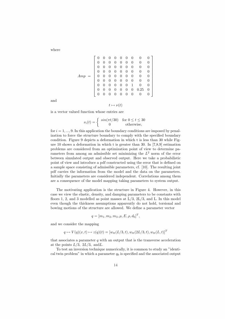
where
Amp =
0 0 0 0 0 0 0 0 00 0 0 0 0 0 0 0 00 0 0 0 0 0 0 0 00 0 0 0 0 0 0 0 00 0 0 0 0 0 0 0 00 0 0 0 0 0 0 0 00 0 0 0 0 0 1 0 00 0 0 0 0 0 0 0.25 00 0 0 0 0 0 0 0 0
andt 7→ ν(t)
is a vector valued function whose entries are
νi(t) =
sin(πt/30) for 0 ≤ t ≤ 300 otherwise,
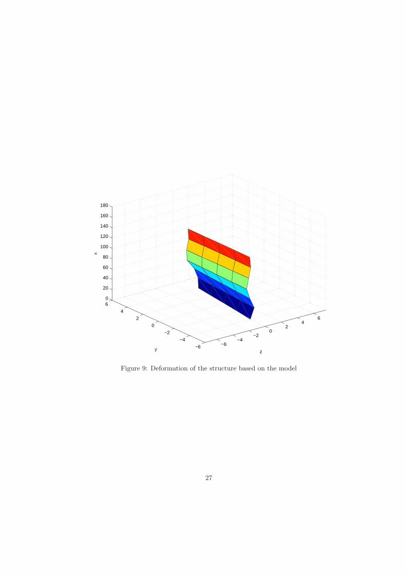
for i = 1, ..., 9. In this application the boundary conditions are imposed by penal-ization to force the structure boundary to comply with the specified boundarycondition. Figure 9 depicts a deformation in which t is less than 30 while Fig-ure 10 shows a deformation in which t is greater than 30. In [7,8,9] estimationproblems are considered from an optimization point of view to determine pa-rameters from among an admissible set minimizing the L2 norm of the errorbetween simulated output and observed output. Here we take a probabilisticpoint of view and introduce a pdf constructed using the error that is defined ona sample space consisting of admissible parameters, cf. [10]. The resulting jointpdf carries the information from the model and the data on the parameters.Initially the parameters are considered independent. Correlations among themare a consequence of the model mapping taking parameters to system output.
The motivating application is the structure in Figure 4. However, in thiscase we view the elastic, density, and damping parameters to be constants withfloors 1, 2, and 3 modelled as point masses at L/3, 2L/3, and L. In this modeleven though the thickness assumptions apparently do not hold, torsional andbowing motions of the structure are allowed. We define a parameter vector
q = [m1,m2,m3, µ, E, ρ, d0]T ,
and we consider the mapping
q 7→ V (q)(x, t) 7→ z(q)(t) = [wtt(L/3, t), wtt(2L/3, t), wtt(L, t)]T
that associates a parameter q with an output that is the transverse accelerationat the points L/3, 2L/3, andL.
To test an inversion technique numerically, it is common to study an ”identi-cal twin problem” in which a parameter q0 is specified and the associated output
14
z0(t) = V (q0)(t) + noise is calculated. This output is then used in the inversionalgorithm to recover the parameter q0, or to determine the information suppliedby the data. This is done by defining a fit-to-data criterion
J(q) =∫ tf
0
(z(q)(t)− z0(t))T M(z(q)(t)− z0(t))dt
expressing the error between computed outputs and the data. A ”solution” ofthe estimation problem is a minimizer of J(q) over the admissible parameter setQ.
In stochastic or probabilistic inversion, a probability density function overthe set Q by
q 7→ f(q) = Cexp[−12J(q)].
The constant C is introduced as a normalization factor so that∫
Q
f(q)dq = 1.
This resulting joint pdf contains information on the parameters from the admis-sible set that is embodied in the data z0(t). It may be used to gain informationon individual or combinations of the parameters through marginalization. Wemay also determine the information gained by comparing probability intervalscalculated from the pdf obtained from the data with those determined withoutdata. This comparison enables us to assess the added value of the data over oura priori information. In addition, using the joint pdf, we can make predictionson the probable behavior of the structure based on available information. Thestructure’s behavior may be viewed as a random variable defined on the sam-ple space Q. Thus, we may compute the distribution for that random variableresulting from the data.
A drawback of the ”identical twin” approach is that many times a givenmethod may work well with some q0, but not with others. Our approach isto view the parameters q0 themselves as random variables and consider an en-semble of problems. If no problem is any more likely than any other, thenthe generating parameters q0 may be considered to be uniformly distributedover the admissible set Q. On the other hand, if there is information indicatingsome problems are more likely than others, then this may be reflected in thechoice of the example problems. Here we view the q0 as uniformly distributedover Q and consider an ensemble of problems chosen randomly over Q using auniformly distributed random number generator. We present ratios of 0.95 prob-ability between a posteriori marginal distributions determined with the benefitof data and marginal distributions obtained without the benefit of additionaldata. These are then averaged over the ensemble of problems to obtain an indi-cator of how much information on a particular parameter is obtained from thedata.
15
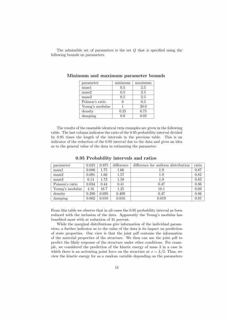
The admissible set of parameters is the set Q that is specified using thefollowing bounds on parameters.
Minimum and maximum parameter bounds
parameter minimum maximummass1 0.5 2.5mass2 0.5 2.5mass3 0.5 2.5Poisson’s ratio 0 0.5Young’s modulus 1 20.0density 0.25 0.75damping 0.0 0.02
The results of the ensemble identical twin examples are given in the followingtable. The last column indicates the ratio of the 0.95 probability interval dividedby 0.95 times the length of the intervals in the previous table. This is anindicator of the reduction of the 0.95 interval due to the data and gives an ideaas to the general value of the data in estimating the parameter.
0.95 Probability intervals and ratios
parameter 0.025 0.975 difference difference for uniform distribution ratiomass1 0.086 1.75 1.66 1.9 0.87mass2 0.091 1.66 1.57 1.9 0.82mass3 0.14 1.73 1.59 1.9 0.83Poisson’s ratio 0.034 0.44 0.41 0.47 0.86Young’s modulus 4.16 16.7 1.25 18.1 0.69density 0.286 0.695 0.409 0.47 0.86damping 0.002 0.018 0.016 0.019 0.85
From this table we observe that in all cases the 0.95 probability interval as beenreduced with the inclusion of the data. Apparently the Young’s modulus hasbenefited most with at reduction of 31 percent.
While the marginal distributions give information of the individual param-eters, a further indicator as to the value of the data is its impact on predictionof state properties. Our view is that the joint pdf contains the informationof the material properties of the structure. We then can use the joint pdf topredict the likely response of the structure under other conditions. For exam-ple, we considered the prediction of the kinetic energy of mass 3 in a case inwhich there is an activating point force on the structure at x = L/2. Thus, weview the kinetic energy for as a random variable depending on the parameters
16

q ∈ Q. As such, the cumulative distribution of the kinetic energy may be cal-culated. In Figure 11 is presented the cumulative distributions obtained in thepresence of data and without the benefit of the data. That is, the a priori pdfas simply the uniform distribution over Q and the a posteriori pdf with dataare used to calculate the distribution of the kinetic energy. The steeper curveis the cdf obtained with data and indicates that there is a probability of 0.95that the kinetic energy is between 0.015 and 0.03. Without the data there is a0.95 probability that the kinetic energy is between 0.01 and 0.12. For this casethe data has brought about a substantial narrowing of the 0.95 interval for thepredicted response of the structure and thereby has substantially increased ourinformation on the state of the system.
17

References
[1] Graff,K.F, Wave Motion in Elastic Solids, Ohio State University Press,Columbus, Ohio, 1975.
[2] Hunter,S.C., Mechanics of Continuous Media, Ellis Horwood, New York,1976.
[3] Matlab Wavelet Toolbox User’s Guide, The Math Works, Inc., 1996.
[4] Mindlin, R.D., Influence of rotatory inertia and shear on flexural motionsof isotropic elastic plates, Journal of Applied Mechanics, March, 1951, pp31-38.
[5] Meirovitch, L., Analytic Methods in Vibrations, MacMillan, London, 1967.
[6] Schultz, M. Spline Analysis, Prentice-Hall, Englewood Cliffs, NJ,1973.
[7] Russell, D. and L. White, Identification of Parameters in Narrow PlateModels from Spectral Data,Journal of Mathematical Analysis and Applica-tions,” 197, (1996),pp 679-707.
[8] Russell, D. and L. White, Formulation and Validation of Dynamical Mod-els for Narrow Plate Motion, Journal Applied Mathematics and Computa-tion,” 58, (1993),pp 103-141.
[9] Russell, D. and L. White, The Bowed Narrow Plate Model, Electronic Jour-nal of Differential Equations,” April(2000).
[10] Tarantola, A., Inverse Problem Theory, Elsevier, New York, 1987.
18
z
y
x
L
0
h −h
k
−k
v
w
u
Figure 1: Formulation of the model
19

z
y
x
L
0
h −h
k
−k
v
w
u
L1
Figure 2: Formulation of the Tip Mass Model
20

0 0.5 1 1.5 2 2.5 3 3.5 4−1
−0.5
0
0.5
1
1.5x 10
−3
time (sec)
disp
lace
men
t (in
)
Solid Affine
Correlation Coefficient = 0.94
Dashed Affine
Solid Euler−Bernoulli
Figure 3: Comparison of tip displacements using the narrow plate and Euler-Bernoulli tip mass models
21

z
y
x
0
L floor 3
floor 2
floor 1
base
−h h
−k
k
w
v
u
Figure 4: Basic structure for laboratory data
22
0 2000 4000 6000 8000 10000 12000 14000 160000.02
0.025
0.03
0.035
0.04
0.045
0.05Base acceleration input into model
time in 0.01 secs
acce
lera
tion
in in
ches
/sec
2
Figure 5: Wavelet approximation of the base acceleration
23
0 2000 4000 6000 8000 10000 12000 14000 16000−0.02
−0.015
−0.01
−0.005
0
0.005
0.01
time in 0.01 secs
Comparison of approximation of the observed acceleration and computed
acce
lera
tion
(in/s
ec2 )
floor 1
dashed observed
solid computed
correlation of the entire signal is 0.64
correlation from 40 to 150 is 0.96
Figure 6: Wavelet approximation of the 1st floor acceleration and the model-computed acceleration
24
0 2000 4000 6000 8000 10000 12000 14000 16000−0.02
−0.015
−0.01
−0.005
0
0.005
0.01
time in 0.01 secs
Comparison of approximation of the observed acceleration and computed
acce
lera
tion
(in/s
ec2 )
floor 2
dashed observed
solid computed
correlation of computed t=70−140to observed t=80−150 is 0.97
correlation of computed t=70−150 to observed t=70−150 without a shift is 0.71
Figure 7: Wavelet approximation of the 2nd floor acceleration and the model-computed acceleration
25
0 2000 4000 6000 8000 10000 12000 14000 16000−0.02
−0.015
−0.01
−0.005
0
0.005
0.01
acce
lera
tion
(in/s
ec2 )
time in 0.01 secs
Comparison of approximation of the observed acceleration and computed
floor 3
dashed observed
solid calculated
correlation from 60−150 is 0.94
Figure 8: Wavelet approximation of the 3rd floor acceleration and the model-computed acceleration
26
−6−4
−20
24
6
−6
−4
−2
0
2
4
60
20
40
60
80
100
120
140
160
180
zy
x
Figure 9: Deformation of the structure based on the model
27

−6−4
−20
24
6
−6
−4
−2
0
2
4
60
20
40
60
80
100
120
140
160
180
zy
x
Figure 10: Deformation of the structure based on the model
28

0 0.02 0.04 0.06 0.08 0.1 0.12 0.14 0.16 0.180
0.1
0.2
0.3
0.4
0.5
0.6
0.7
0.8
0.9
1
Pro
babi
lity
Kinetic energy
Figure 11: Cumulative distribution of the kinetic energy at mass 3
29