John UrbanicParallel Computing Scientist

Pittsburgh Supercomputing Center

Copyright 2017

A Recommender System

Obvious ApplicationsWe are now advanced enough that we can aspire to a serious application. One of the most significant applications for some very large websites (Netflix, Amazon, etc.) are recommender systems.

“Customers who bought this product also bought these.”

“Here are some movies you might like…”

As well as many types of targeted advertising. However those of you with less commercial ambitions will find the core concepts here widely applicable to many types of data that require dimensionality reduction techniques.

Let’s go all Netflix

1) https://en.wikipedia.org/wiki/Netflix_Prize

Netflix once (2009) had a $1,000,000 contest to with just this very problem(1). We will start with a similar dataset. It looks like:

Movie Dataset (Movie ID, Title, Genre):31,Dangerous Minds (1995),Drama32,Twelve Monkeys (a.k.a. 12 Monkeys) (1995),Mystery|Sci-Fi|Thriller34,Babe (1995),Children|Drama

Ratings Dataset (User ID, Movie ID, Rating, Timestamp):2,144,3.0,8353560162,150,5.0,8353553952,153,4.0,8353554412,161,3.0,835355493

We won’t use the genres or timestamp fields for our analysis.

ObjectiveFor any given user we would like to use their ratings, in combination with all the existing user ratings, to determine which movies they might prefer. For example, a user might really like Annie Hall and The Purple Rose of Cairo (both Woody Allen movies, although our database doesn’t have that information). Can we infer from other users that they might like Zelig? That would be finding a latent variable. These might also include affinities for an actor, or director, or genre, etc.

So what we have is a (sparse) list of ratings for a user:

2 4 5 3

Black BoxWe want to run that through a black box and get a list of projected ratings.

2 4 5 3

3 2 6 4 1 3 1 5 2 8 4 5 3 2 3 4 3 4 2

Matrix MultiplyThis might have the feel of a matrix multiply. Linear algebra is the language of machine learning, but you won’t need to do more than recall the basics today.

=

This isn’t our answer. It would be difficult for such a matrix to deal with the sparsity of the input vector for one thing. We can do something even more direct.

User Item Association MatrixWe will construct a matrix to that is simply a spreadsheet that contains all of our users’ projected ratings.

3 2 6 4 1 3 1 5 2 8 4 5 3

4 5 2 1 2 4 3 4 5 4 1 5 2

This will be a very large matrix (all movies X all users). The way we construct it will allow us to save it in a much more compact form.

Lossy Compression Becomes Approximate Solution

The answer to the problem of compressing this matrix to a reasonable size is also going to provide us a means to construct it.

UR PX

We are going to approximate our given, sparse, R matrix as the product of two smaller matrices. You can consider them a user feature matrix and an item feature matrix. This approximation is also going to smooth out the zeros and in the process give us our projected ratings. But we’ll get to that.

Matrix FactorizationThere are different ways to decompose a matrix. We will approximate this matrix as the product of two smaller matrices. The rank, k, of the new matrices will determine how many effects we are incorporating.

UR PX

k

k

Why not SVD?For those of you familiar with these kinds of techniques, you may wonder why we aren’t using Singular Value Decomposition. This is another common technique to decompose matrices and is also part of Spark’s mllib.

SVD reduces the matrix to three submatrices, a diagonal matrix and two orthonormal matrices. These have some nice properties to work with.

However, there are two major drawbacks for this application:

• More expensive, which matters for these potentially immense matrices.• Original matrix must be dense. Our given matrix will have lots of missing values

(corresponding to the many unrated movies for any user).

Defining our error

In ML, defining the error (or loss, or cost) is often the core of defining the objective solution. Once we define the error, we can usually plug it into a canned solver which can minimize it. Defining the error can be obvious, or very subtle.

Clustering: For k-means we simply used the geometrical distance. It was actually the sum of the squared distances, but you get the idea.

Image Recognition: If our algorithm tags a picture of a cat as a dog, is that a larger error than if it tags it as a horse? Or a car? How would you quantify these?

Recommender: We will take the Mean Square Error distance between our given matrix and our approximation as a starting point.

Mean Square Error plus RegularizationWe will also add a term to discourage overfitting by damping large elements of U or P. This is called regularization and versions appear frequently in error functions. MLLIB scales this factor for us based on the number of ratings (this tweak is called ALS-WR).

Error = R – UxP 2 + (U2 + P2)

The notation means “sum the squares of all the elements and then take the square root”.

Additionally, we need to account for our missing (unrated) values. We just zero out those terms. Here it is term-by-term:

Error = I,j wI,j (RI,j – (UxP)ij)2 + (U2 + P2) wI,j =0 if RI,j is unknown

Note that we now have two parameters, k and , that we need to select intelligently.

You may wonder how we can have “too little” error – the pursuit of which leads to overfitting. Think back to our clustering

problem. We could drive the error as low as we wanted by adding more clusters (up to 5000!). But we weren’t really finding new

clusters.

We use the training data to create our solution, the UxP matrix here.

The validation data is used to verify we are not overfitting: to stop training after enough iterations, to adjust or k here, or to

optimize the many other hyperparameters you will encounter in ML.

The test data must be saved to judge our final solution.

Reusing, or subtly mixing, the training, validation and test data is a frequently cause of confusion.

Overfitting

One solution is to keep using

higher order terms, but to

penalize them. These

regularization hyperparameters

that enable our solution to

have good generalization will

show up again in our

workshop, and throughout your

machine learning endeavors.

Alternating Least SquaresTo actually find the U and P that minimize this error we need a solving algorithm.

SGD, a go-to for many ML problems and one we will use later, is not practical for billions of parameters, which we can easily reach with these types of problems. We are dealing with Users X Items elements here.

Instead we use Alternating Least Squares (ALS), also built into MLLIB.

• Alternating least squares cheats by holding one of the arrays constant and then doing a classic least squares fit on the other array parameters. Then it does this for the other array.

• This is easily parallelized.

• It works well with sparse inputs. The algorithm scales linearly with observed entries.

Here Is Our Plan

UPX

Given

Ratings

Sparse

Use

ALS

Predicted

Ratings

Dense

=

Let’s Build A RecommenderWe have all the tools we need, so let’s fire up PySpark and make create a scalable recommender. Our plan is:

1. Load and parse data files2. Create ALS model3. Train it with varying ranks (k) to find reasonable values

4. Add a new user5. Get top recommendations for new user

____ __/ __/__ ___ _____/ /__

_\ \/ _ \/ _ `/ __/ '_//__ / .__/\_,_/_/ /_/\_\ version 1.6.0

/_/

Using Python version 2.7.5 (default, Nov 20 2015 02:00:19)SparkContext available as sc, HiveContext available as sqlContext.>>>>>> ratings_raw_RDD = sc.textFile('ratings.csv')>>> ratings_RDD = ratings_raw_RDD.map(lambda line: line.split(",")).map(lambda tokens: (int(tokens[0]),int(tokens[1]),float(tokens[2])))>>>>>> training_RDD, validation_RDD, test_RDD = ratings_RDD.randomSplit([3, 1, 1], 0)>>>>>> predict_validation_RDD = validation_RDD.map(lambda x: (x[0], x[1]))>>> predict_test_RDD = test_RDD.map(lambda x: (x[0], x[1]))

Building a Recommender

We load in the ratings file and parse out the (user,movie,rating) data.

We then split it training, validation and test data RDDs.

Then we strip the ratings off the validation and test data for our prediction RDDs.

>>> training_RDD.take(4)[(1, 1029, 3.0), (1, 1061, 3.0), (1, 1263, 2.0), (1, 1371, 2.5)]>>> predict_validation_RDD.take(4)[(1, 1129), (1, 1172), (1, 1405), (1, 2105)]>>>

br06% interact...r288% r288% module load sparkr288% pyspark

____ __/ __/__ ___ _____/ /__

_\ \/ _ \/ _ `/ __/ '_//__ / .__/\_,_/_/ /_/\_\ version 1.6.0

/_/

Using Python version 2.7.5 (default, Nov 20 2015 02:00:19)SparkContext available as sc, HiveContext available as sqlContext.>>>>>> ratings_raw_RDD = sc.textFile('ratings.csv')>>> ratings_RDD = ratings_raw_RDD.map(lambda line: line.split(",")).map(lambda tokens: (int(tokens[0]),int(tokens[1]),float(tokens[2])))>>>>>> training_RDD, validation_RDD, test_RDD = ratings_RDD.randomSplit([3, 1, 1], 0)>>>>>> predict_validation_RDD = validation_RDD.map(lambda x: (x[0], x[1]))>>> predict_test_RDD = test_RDD.map(lambda x: (x[0], x[1]))>>>>>>>>> from pyspark.mllib.recommendation import ALS>>> import math>>>>>> seed = 5>>> iterations = 10>>> regularization = 0.1>>> ranks = [4, 8, 12]>>> errors = [0, 0, 0]>>> err = 0>>> tolerance = 0.02>>> min_error = float('inf')>>> best_rank = -1

Import mllib and set some variables we are about to use.

>>> ratings_raw_RDD = sc.textFile('ratings.csv')>>> ratings_RDD = ratings_raw_RDD.map(lambda line: line.split(",")).map(lambda tokens: (int(tokens[0]),int(tokens[1]),float(tokens[2])))>>>>>> training_RDD, validation_RDD, test_RDD = ratings_RDD.randomSplit([3, 1, 1], 0)>>>>>> predict_validation_RDD = validation_RDD.map(lambda x: (x[0], x[1]))>>> predict_test_RDD = test_RDD.map(lambda x: (x[0], x[1]))>>>>>>>>> from pyspark.mllib.recommendation import ALS>>> import math>>>>>> seed = 5>>> iterations = 10>>> regularization = 0.1>>> ranks = [4, 8, 12]>>> errors = [0, 0, 0]>>> err = 0>>> tolerance = 0.02>>> min_error = float('inf')>>> best_rank = -1>>>>>> for rank in ranks:>>> model = ALS.train(training_RDD, rank, seed=seed, iterations=iterations, lambda_=regularization)>>> predictions_RDD = model.predictAll(predict_validation_RDD).map(lambda r: ((r[0], r[1]), r[2]))>>> ratings_and_preds_RDD = validation_RDD.map(lambda r: ((r[0], r[1]), r[2])).join(predictions_RDD)>>> error = math.sqrt(ratings_and_preds_RDD.map(lambda r: (r[1][0] - r[1][1])**2).mean())>>> errors[err] = error>>> err += 1>>> print 'For rank %s the RMSE is %s' % (rank, error)>>> if error < min_error:>>> min_error = error>>> best_rank = rank>>>For rank 4 the RMSE is 0.93683749317For rank 8 the RMSE is 0.952092733983For rank 12 the RMSE is 0.951914636563>>>>>> print 'The best model was trained with rank %s' % best_rankThe best model was trained with rank 4

Run our ALS model on various ranks to see which is best.

>>>>>> for rank in ranks:>>> model = ALS.train(training_RDD, rank, seed=seed, iterations=iterations, lambda_=regularization)>>> predictions_RDD = model.predictAll(predict_validation_RDD).map(lambda r: ((r[0], r[1]), r[2]))>>> ratings_and_preds_RDD = validation_RDD.map(lambda r: ((r[0], r[1]), r[2])).join(predictions_RDD)>>> error = math.sqrt(ratings_and_preds_RDD.map(lambda r: (r[1][0] - r[1][1])**2).mean())>>> errors[err] = error>>> err += 1>>> print 'For rank %s the RMSE is %s' % (rank, error)>>> if error < min_error:>>> min_error = error>>> best_rank = rank>>>>>> print 'The best model was trained with rank %s' % best_rank>>>For rank 4 the RMSE is 0.93683749317For rank 8 the RMSE is 0.952092733983For rank 12 the RMSE is 0.951914636563>>>The best model was trained with rank 4

>>> model.predictAll(predict_validation_RDD).take(2)[Rating(user=463, product=4844, rating=2.7640960482284322), Rating(user=380, product=4844, rating=2.399938320644199)]>>>>>> model.predictAll(predict_validation_RDD).map(lambda r: ((r[0], r[1]), r[2])).take(2) # predictions_RDD[((463, 4844), 2.7640960482284322), ((380, 4844), 2.399938320644199)]>>>>>> validation_RDD.take(2)[(1, 1129, 2.0), (1, 1172, 4.0)]>>> >>> validation_RDD.map(lambda r: ((r[0], r[1]), r[2])).take(2)[((1, 1129), 2.0), ((1, 1172), 4.0)]

>>> predictions_RDD.take(2)[((463, 4844), 2.7640960482284322), ((380, 4844), 2.399938320644199)]>>>>>> validation_RDD.map(lambda r: ((r[0], r[1]), r[2])).take(2)[((1, 1129), 2.0), ((1, 1172), 4.0)]>>>>>> ratings_and_preds_RDD.take(2) # validation_RDD joined predictions_RDD[((119, 145), (4.0, 2.903215714486778)), ((407, 5995), (4.5, 4.604779028840272))]

>>> for rank in ranks:>>> model = ALS.train(training_RDD, rank, seed=seed, iterations=iterations, lambda_=regularization)>>> predictions_RDD = model.predictAll(predict_validation_RDD).map(lambda r: ((r[0], r[1]), r[2]))>>> ratings_and_preds_RDD = validation_RDD.map(lambda r: ((r[0], r[1]), r[2])).join(predictions_RDD)>>> error = math.sqrt(ratings_and_preds_RDD.map(lambda r: (r[1][0] - r[1][1])**2).mean())>>> errors[err] = error>>> err += 1>>> print 'For rank %s the RMSE is %s' % (rank, error)>>> if error < min_error:>>> min_error = error>>> best_rank = rank>>>>>> print 'The best model was trained with rank %s' % best_rank>>>For rank 4 the RMSE is 0.93683749317For rank 8 the RMSE is 0.952092733983For rank 12 the RMSE is 0.951914636563>>>The best model was trained with rank 4>>>>>> model = ALS.train(training_RDD, best_rank, seed=seed, iterations=iterations, lambda_=regularization)>>> predictions_RDD = model.predictAll(predict_test_RDD).map(lambda r: ((r[0], r[1]), r[2]))>>> ratings_and_preds_RDD = test_RDD.map(lambda r: ((r[0], r[1]), r[2])).join(predictions_RDD)>>> error = math.sqrt(ratings_and_preds_RDD.map(lambda r: (r[1][0] - r[1][1])**2).mean())>>> print 'For testing data the RMSE is %s' % (error)>>> For testing data the RMSE is 0.932684762873

This is our fully tested model (smallest dataset).

.

.

.>>>>>> new_user_ID = 0>>> new_user = [

(0,100,4), # City Hall (1996)(0,237,1), # Forget Paris (1995)(0,44,4), # Mortal Kombat (1995)(0,25,5), # etc....(0,456,3),(0,849,3),(0,778,2),(0,909,3),(0,478,5),(0,248,4)]

>>>>>> new_user_RDD = sc.parallelize(new_user)>>> updated_ratings_RDD = ratings_RDD.union(new_user_RDD)>>>>>> updated_model = ALS.train(updated_ratings_RDD, best_rank, seed=seed, iterations=iterations, lambda_=regularization)>>>

Adding a User

We assume User ID 0 is unused, but could check withratings_RDD.filter(lambda x: x[0]=='0').count()"

.

.

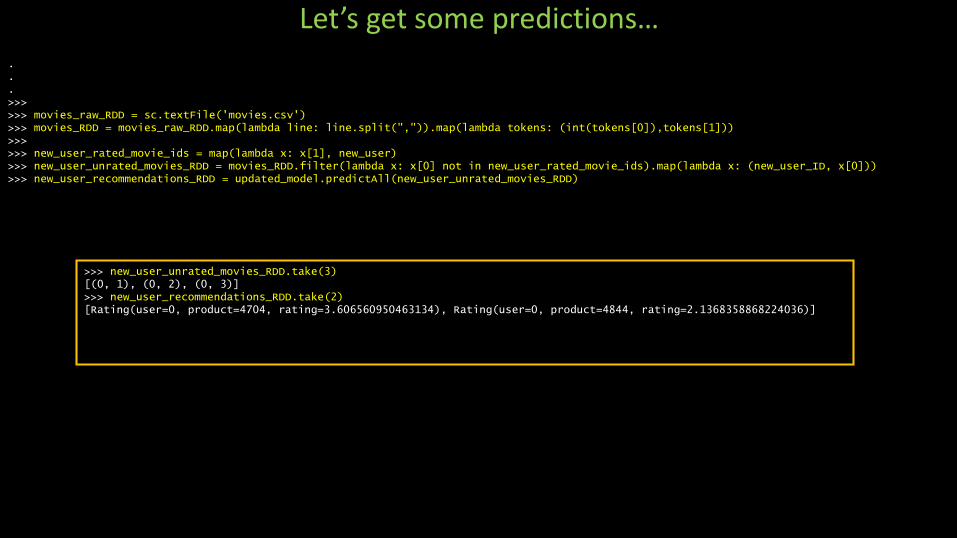
.>>>>>> movies_raw_RDD = sc.textFile('movies.csv')>>> movies_RDD = movies_raw_RDD.map(lambda line: line.split(",")).map(lambda tokens: (int(tokens[0]),tokens[1]))>>>>>> new_user_rated_movie_ids = map(lambda x: x[1], new_user)>>> new_user_unrated_movies_RDD = movies_RDD.filter(lambda x: x[0] not in new_user_rated_movie_ids).map(lambda x: (new_user_ID, x[0]))>>> new_user_recommendations_RDD = updated_model.predictAll(new_user_unrated_movies_RDD)

Let’s get some predictions…

>>> new_user_unrated_movies_RDD.take(3)[(0, 1), (0, 2), (0, 3)]>>> new_user_recommendations_RDD.take(2)[Rating(user=0, product=4704, rating=3.606560950463134), Rating(user=0, product=4844, rating=2.1368358868224036)]

.

.

.>>>>>> product_rating_RDD = new_user_recommendations_RDD.map(lambda x: (x.product, x.rating))>>> new_user_recommendations_titled_RDD = product_rating_RDD.join(movies_RDD)>>> new_user_recommendations_formatted_RDD = new_user_recommendations_titled_RDD.map(lambda x: (x[1][1],x[1][0]))>>>>>> top_recomends = new_user_recommendations_formatted_RDD.takeOrdered(10, key=lambda x: -x[1])>>> for line in top_recomends: print line... (u'Maelstr\xf6m (2000)', 6.2119957527973355)(u'"King Is Alive', 6.2119957527973355)(u'Innocence (2000)', 6.2119957527973355)(u'Dangerous Beauty (1998)', 6.189751978239315)(u'"Bad and the Beautiful', 6.005879185976944)(u"Taste of Cherry (Ta'm e guilass) (1997)", 5.96074819887891)(u'The Lair of the White Worm (1988)', 5.958594728894122)(u"Mifune's Last Song (Mifunes sidste sang) (1999)", 5.934820295566816)(u'"Business of Strangers', 5.899232655788708)>>>>>> one_movie_RDD = sc.parallelize([(0, 800)]) # Lone Star (1996)>>> rating_RDD = updated_model.predictAll(one_movie_RDD)>>> rating_RDD.take(1)[Rating(user=0, product=800, rating=4.100848893773136)]

Let see some titles

>>> new_user_recommendations_titled_RDD.take(2)[(111360, (1.0666741148393921, u'Lucy (2014)')), (49530, (1.8020006042285814, u'Blood Diamond (2006)'))]>>> new_user_recommendations_formatted_RDD.take(2) [(u'Lucy (2014)', 1.0666741148393921), (u'Blood Diamond (2006)', 1.8020006042285814)]

Looks like we can sort by value after all! Behind the scenes takeOredered() just does the key swap and SortByKey that we did ourselves.

Exercises

1) We noticed that out top ranked movies have ratings higher than 5. This makes perfect sense as there is no ceiling implied in our algorithm and one can imagine that certain combinations of factors would combine to create “better than anything you’ve seen yet” ratings.

Maybe you have a friend that really likes Anime. Many of her ratings for Anime are 5. And she really likes Scarlett Johansson and gives her movies lots of 5s. Wouldn’t it be fair to consider her rating for Ghost in the Shell to be a 7/5?

Nevertheless, we may have to constrain our ratings to a 1-5 range. Can you normalize the output from our recommender such that our new users only sees ratings in that range?

2) We haven’t really investigated our convergence rate. We specify 10 iterations, but is that reasonable? Graph your error against iterations and see if that is a good numer.

3) I mentioned that our larger dataset does benefit from a rank of 12 instead of 4 (as one might expect). The larger datasets (ratings-large.csv and movies-large.csv) are available to you. Prove that the error is less with a larger rank. How does this dataset benefit from more iterations? Is it more effective to spend the computation cycles on more iterations or larger ranks?

More Powerful Cluster

If you are going to user the larger datasets, you might want to try with a larger cluster (backed by HDFS). We are giving you all access to the cluster located at r741 (ssh r741 from the bridges front end) for the next two weeks.

Exercises

1) We noticed that out top ranked movies have ratings higher than 5. This makes perfect sense as there is no ceiling implied in our algorithm and one can imagine that certain combinations of factors would combine to create “better than anything you’ve seen yet” ratings.

Maybe you have a friend that really likes Anime. Many of her ratings for Anime are 5. And she really likes Scarlett Johansson and gives her movies lots of 5s. Wouldn’t it be fair to consider her rating for Ghost in the Shell to be a 7/5?

Nevertheless, we may have to constrain our ratings to a 1-5 range. Can you normalize the output from our recommender such that our new users only sees ratings in that range?

2) We haven’t really investigated our convergence rate. We specify 10 iterations, but is that reasonable? Graph your error against iterations and see if that is a good numer.

3) I mentioned that our larger dataset does benefit from a rank of 12 instead of 4 (as one might expect). The larger datasets (ratings-large.csv and movies-large.csv) are available to you. Prove that the error is less with a larger rank. How does this dataset benefit from more iterations? Is it more effective to spend the computation cycles on more iterations or larger ranks?