:~i~N ~9 0 -,

-~~lTATlONI! ~OJECT

IN CENTRAL TUNISIAOperated by

CDM and Associates - -

Sponsored by the U S. Agencyfor International Development

1611 N. Kent Street, Room 1001Arlington, VA 22209-2111 USA

Telephone: (703) 243-8200Fax (703) 525-9137Telex WUI 64552

Cable Address WASHAID

WASH

L18RA~. -

TbREFERENCE

CENT~FOR ~ WATER SUPPL.~AND

FIELD REPORT NO. 298

APRIL 1990

The WASH Project isby Camp Dresser &International Inc. PririclpaJcooperating institutiori~dc~subcontractors are: Assädiáfê~,in Rural Developrn~nt~li~~International Scienc.~:ii~d~Technology lnstitu~e~~Research Triangle !nstitutt~Training Resources r~.çi~University of North C~lit~.at Chapel Hill UniverSi~y~Research Corporation

L~L

Prepared - forthe USAID Mission to Tunisia and

the Central Tunisia Development Authority (CTDA )WASH Task No. 057 and 130

824—TN—7394

A RE - EXAMINATION

OF COSTS

OF RURAL WATER SUPPLY

AND BENEFITS

PROJECTS

WASH Field ReportNo. 298

A RE-EXAMINATION OF COSTSAND BENEFITSOF RURAL WATER SUPPLY PROJECTS

IN CENTRAL TUNISIA

Preparedfor theUSAID Mission to Tunisiaarid theCentralTunisiaDevelopmentAuthority (CTDA)

underWASH TaskNo. 057 and 130

by

Alan Wyatt

April 1990

Water and Sanitation for Health ProjectContract No.5973-7-00-8081-00, Project No. 836-1249

ía sponaored by the Office of Health, Bureau for Science and TechnologyU.S. Agencyfor International Development

Waahington, DC 20523

LIBRARY, INTERNATIONAL REFERENCECENTRE FOR COMMUNITY WATER SUPPLYAND SANWfATION (IRC)P.O. Box 93190, 2509 AD Th~HagueTeL (070) 814911 ext. 141/142

pZc~L~~e~-LL ~N Ojb

RELATED WASH REPORTS

Organization of a Colloquiumon Rural WaterSupplyandSanitation,Kasserlne,Tunisia,byFredRosensweigandRaymondB. lsley. January1983. Field ReportNo. 67.

Evaluation of Health and Social Benefit of Springs Cappedfor Irrigation, Further Adaptedfor Domestic Use In Central Tunisia, by Raymond B. Isley. May 1983. Field ReportNo. 84.

Midterm Evaluation of the USAID/Tunisia Rural Potable WaterInstitutionsProject,by LeeJennings,Ridha Boukraa,MohamedFrloui, Richard Swanson,SereenThaddeus, andAlan Wyatt. July 1989. Field ReportNo. 256. (French and English)

Plan de Travail de L’Unlte d’Autogestlon, by Lee Jennings,Sereen Thaddeus, and AlanWyatt. September 1989. Field Report No. 276. (French only)

Health and Hygiene Educationand Women’s Involvement in the Tunisia Rural Potable WaterInstitutionsProject, by SereenThaddeus. November1989. Field ReportNo. 277.(French and English)

Engineering Design Considerations: Tunisia Rural PotableWater Institutions Project, byAlan Wyatt. November 1989. Field ReportNo. 279. (French and English)

CHAPTER

CONTENTS

ACKNOWLEDGEMENTS.ACRONYMSEXECUTIVE SUMMARY

1. INTRODUCTION

2. BACKGROUND INFORMATION ON ThEAREA

3. PR~OUSECONOMIC STUDIES

3.1 FirstiDAStudy3.2 Second IDA Study3.3 AnalysIsof ProjectZone of Service

4. UPDATED COSTS

5 BENEFIT CALCULATIONS

5.1 IDA Approach

5.2 The RevisedApproach

6. RESULTS

6.1 Comparison of Benefitsand Costs

6.2 Results—ModelSensitivity

7. APPUCATION OF RESULTS

7.1 Evaluationof ProposedSites

7.2 GeneralSite SelectionTables

8. PERSPECTIVES AND CONCLUSIONS

REFERENCES

3

5

567

9

15

1516

23

2328

33

3333

41

43

Page

iiiv

~rn

PROJECTAND ThE PROJECT

APPENDIX

A. Model of Water Point/Water TransportCosts 47B. Resultsof SensitivityAnalyses 57C. Detailed Benefit/CostResultsfor Early ProjectSites 65D. DetailedBenefit/CostResultsfor Candidate Project Sites 73

TABLE

1. Overall Cost Model 102. Assumptionsand Sources 113. CalculatedValuesand Formulas 124. Basic Input Output Computer Screen 245. Initial Benefit and Cost Calculations 256. Benefit/CostTabulation 267. EconomIc Analysisof ProposedSites 358. Results- Benefit/Cost Ratio 369. Results- Benefit/CostRatio 3710. Results- Benefit/CostRatio 3811. Results- internalRate of Return 3912. Project SelectionMatrix 40

FIGURE

1. Model Results 272. Sensiti(’ity to Accounting Ratios 313. Minimum Required Population by Well Depth 40

BOX

1. Report Purpose 22. Key DifferencesbetweentheNew Cost Model andIDA’s 143. Population Computation 174. Time SavingsComputation 185. Value of Time Estimation 206. BenefitsComputation 217. Comparison of EconomicAnalyses 288. SensItivity of the EconomicAnalysisModel 30

11

ACKNOWLEDGEMENTS

This working paper hasinvolved the Input of many Individuals who deservea word ofthanksMost of all I must thank thestaff at CTDA who worked with me on this effort. M. Charfi ofthePlanning and Evaluation Office (DPE~deservesspecial credit for his careful examinationof the benefits calculations, and his approach to defining the project radius which isincorporatedhere.Thanksalsomustgo to Moncef Hussein,BelgacemKhessaissia,MokhdedMissaoui,Haul Mosbah,and Khaled Sanounof AUI whoreviewedworksheetcalculationsanddiscussedvarious pointswith me. Thanks must go to Diana Putmanof USAID/Tunis whooverseesthis project so carefully and has supported this work. Lastly, I must thank DaleWhittington of UNC, who reviewedan early draft andgavevaluable comments,and JaneWalker of WASH, who also provided useful inputto this work.

ABOUT TI-fE AUThOR

Alan Wyatt is a mechanicalengineer who has experiencein the technical and economicaspectsof rural water supply in developing countries. He has worked on water supplyprojects in Haiti, Honduras, Mali, Morocco, and Tunisia. He participatedin the midtermevaluationof the Rural Potable Water Supply InstitutionsProject in February 1989, and hassinceconducted two follow-up missionsto the project in Kasserine.

iii

ACRONYMS

AIRD Associatesfor internationalResourcesand Development

B/C beneftVcost

CRDA RegionalCommissionfor Agricultural Development

CTDA Central Tunisia DevelopmentAuthority

g/1 gallons/liter

IDA Institute for DevelopmentAuthority

IRR internal rate of return

lpcd liters per capitaperday

km kilometer

I liter

m meter

mm millimeter

SCE1’ a Tunisian consultingfirm

TD Tunisian dinar (exchangerate in February 1989 was lTD — $1.09 or

$1 ..0.92TD)USAID U.S. Agency for InternationalDevelopment

WASH Water and Sanitation for HealthProject

V

EXECUTIVE SUMMARY

This paper describesa benefit/cost(B/C) model developedfor theRegional CommissionforAgricultural Development (CRDA) of the USAID-funded Rural Potable Water InstitutionsProjectin Kasserine,Tunisia, in responseto one of the principal objectivesof the project:to maximize water investments by improving site selection for new and Improved watersystems. The model is usedto allocate Investment funds for rural water supply projects,according to a rankingof candidate sitesbasedon the B/C criterion. It wasdevelopedbyWASH and CRDA staff under a technicalassistanceprogramdelivered under the WASHproject. The analysisis basedon earlier work, but hasupdatedcostdata and takes a newapproach to the assessmentof benefits,asa result of which the projects are shownto havegreater economicfeasibility. However, this analysisis preliminary andbasedon limited data.A plannedsurvey of water usersis expectedto yield additional data to refine the benefitscalculation. Nonethelessthis analysisshouldhelp the project staff to makesound invesfrnentdecisions.

In 1987,a report on theeconomicfeasibility of rural water projects preparedby the Institutefor DevelopmentAnthropology(IDA) computed the B/C ratio and Internal rate of return(IRR) for typical project sites. B/C ratiosranged from 0.69 to 1.65,and IRR valuesfrom8 to 35 percent. The siteswith higher well depths and lower populations did the poorest,while those with oppositeconditions produced the besteconomicfeasibility.

IDA’s calculation of benefits wasmadefrom time savingsfor usersand an estimateof theeconomicvalueof time, basedon a small surveyof rural water usersIn 1985. Someaspectsof the calculationare questionable. All sitesare assumedto yield uniform benefits,whethertheyare near or far from an existing source, and the benefits are assumedto derive onlyfrom time savingsby men,which seemswrong and short-sighted.

The model describedhere is based on more recent cost data. It is driven by thecharacteristicsof the candidate site—population, water consumption, estimatedwelldepth—and computesfull Investment costs. Theseare high—mostly becausedrilled wellscost350Thper m of depth, and wellsare typically over 300 m deep. Thus, thewell alonecould cost more than 100,000TD. O&M costs over a 20-year period are based onengineeringcalculationsand historical data, and Include thesalariesof governmentpersonnelinvolved in establishingarid maintaining the systems. The model usesaccounting ratios tocalculateeconomiccostsfrom market prices, basedon previouseconomicstudiesfor Tunisia

This revisedmodelalso usestravel time savingsasthe basicbenefit, but with an empiricalestimateof the value of time derivedfrom the overall behaviorof the rural population in theregion. The new value of time is higher thanin previous estimates,and is independentofthe persontraveling and of the intended useof water. The resultingbenefitsper family peryearare higher than previously estimated. Although it is basedon limited aggregatedata,the revisedapproach reflects people’sown valuationof benefits. It assesseswhat families

vii

are willing to pay in time or cashfor water. A more predseassessmentof project benefitscan be expectedfrom the resultsof the upcoming rural householdsurvey.

A recalculationof benefitsat sitesstudiedin the IDA reportprovided a comparison betweenthe two analyses.The newanalysis yields consistently higher lRRs thatcanbe attributedmostly to increasedbenefits resulting from the Increasedvalue of time. The model wasapplied to sitesbeing considered for the next cyde of projects. As expected,the moreeconomicallyattractive siteshavehigher populations,lower well depths,and longer (current)travel distancesto water. B/C valuesranged from 0.94 to 2.74 andIRR valuesfrom 10percent to 44 percent. Thesesiteshave been rankedaccording to the B/C criterion, andare being implemented accordingly. Despite the preliminary nature of the benefitscalculations, the B/C model can be tentatively applied to the task of general projectselection.A setof tableshasbeenprepared for rapid economicappraisal of future projects.The original project selectioncriteriawerereviewed and an alternative approach basedonthis model hasbeen proposed.

In summary,a revisedB/C approach hasbeendevelopedto assistin selectingproject sitesand maximizing investments. The resultsshow that the economicfeasibility of rural waterprojects may be better than previously estimated. This model should be updatedwhenadditional data on benefitshave beencollected. Also, the modelcan be applied to the taskof studyingand improving engineeringdesignsusedin the project.

viii

Chapter 1

INTRODUCTION

One of the principal objectivesof the Rural Potable Water Institutions Project is to maximizewater investmentsby Improving site selectionfor newand improved water systems.To thisend, a number of studies have beenconducted over the past few yearsby the CentralTunisian DevelopmentAuthority (CTDA) and the Institute for DevelopmentAnthropology(IDA). Theseefforts includedemographic studies,hydro-geologicstudies, thewater resourcesmappingstudies(induding a series of acetateoverlay maps), studies on the site selectionprocess,aswell as project economicanalyses.There is little doubt that all theseinputshaveimproved the CTDA’s selectionof sitesfor water systemdevelopment.

The essenceof the site selectionissueis that the available project funding be spentto do themost good. There are numerousways of deciding how to allocate project resources. Oneapproachwould be to install water systemsin the driest areas—thezoneswhere populationsare large, but goodwatersourcesare very far away. But to selectsiteson the basisof pureneed (whith could be equatedwith benefits) would be a poor way to allocateresourcesifcostswere not taken Into account. For example, wherethere are two siteswith equalneedsbut different costs,the lower costsite should be rankedfirst. The traditional approach toallocationsof this type is to usethe benefit/cost (B/C) ratio, or the Internal rate of return(IRR) to set priorities amongcandidate sites. Previous project economicanalysesby IDA(Reeser1987,and Reeser1988)have usedthis approach.

In early 1989, as the engineer on the mid-term evaluation team, the consultant had theopportunity to review previous IDA/CTDA economicanalyses.While theyseemedto bebasically sound, there were someaspectswhich were out of date (particularly costs), aridsome which seemedunconventional (particularly benefits). In addition, the local projectimplementation teamwasnot really using the resultsor methodology of theseanalysesinproject selection.In fact, somesiteswhich appearedeconomicallyquestionablewere beingdeveloped. Thus it was decided to rework someof the calculations and re-examine theresults. In June 1989, thesemodificationswere reviewed with the CTDA staff, additionalchanges were made, and a revised approach was adopted. On a return visit by theconsultant In August 1989,further minor refinementswere agreedto. This report describesthat updated approach. Its purposesare summarized In Box 1.

1

REPORT PURPOSES

Box 1

Thisapproach must still be consideredpreliminary. The calculation for assessmentof benefitsis basedon limited data and severalkey assumptions.Field surveyswill be neededto collectsufficient data for a more accurate calculation of project benefits. Nonethelessthe currentmodel givesa goodapproachfor choosingbetweencandidatesites.Future changesin benefitcalculationswould probably affect all sitesequally, so the resultsof prioritizing siteswould beunchanged.The current model cannotdefinitively answerwhether, or to what extent, thesesitesare economically feasible(B/C> 1). Changesto benefit calculationswill impact B/Cratiosand IRRs, so thatsiteswhich now appear feasiblemaynot seemsoin the future. Thecurrent model is valid for relativesite analyses(choosinghowto allocate resourcesbetweensites), but not for absoluteanalyses(determining site economicfeasibility, establishing newsite selectioncriteria, or comparingthe economicfeasibility of rural water supply versusinvestmentsin schools,roads, agriculture projects, or other usesof developmentresources).The current model doesgive preliminary indicationson theseabsoluteeconomicissues.

• To update previous studieswith more recent cost information

• To re-examinepreviousbenefit calculations

• To re-compute benefit/cost ratios for typical projects, andevaluatedifferences with previous efforts

• To examinemodel sensitivity to assumedparameters for costandbenefits

• To apply theanalysisprocedures to sevencandidate sites,andprioritize them

• To developsimple tables of economicanalysisresultsfor useinthe site selectionprocess

2

Chapter 2

BACKGROUND INFORMATION ON ThE PROJECTAND THE PROJECTAREA

The USAID/CTDA project area lies in Central Tunisia, and indudes the Govemorate ofKasserineand the northern partof the Governorate of Gafsa.The areaconsistsof semi-aridhigh steppes,with an annualrainfall rangingfrom 200to 400 mm. In general,the south Isdrier than the north.

The population of the region is about 300,000,wIth approximately half In rural and half inurban areas.Beforethe colonial period the local Inhabitantswerenomads,grazing sheepandgoats in winter, and moving into Northern Tunisia in the hot dry summer. During thecolonial period and later, efforts were made to settle them and encourage dry landagriculture.Today,rural dwellersstill tend livestockandengagein farming (irrigated in somecases).Many have family memberswho have left the region for employment In the coastalcities or in Europe.

The rural population is highly dispersed. Densities outside towns is typically around 30p/km2. Peopleoften live within 5 to 15 km of a centerwhere a school, mosque, waterpoint, or other servicesmaybe found.

Water resourcesin thearea are not plentiful. There are very few surface water sources.Attheedgeof hillsidesand ridges, springsare occasionallyfound. In someareas,such asSbibafor example,a phreaticaquifer can be found at depths of under 50 m, but manyareashaveonly deepaquifers or no groundwater at all. In many areasreasonablequantities of watercan be found only at depths of 300-400m, and asdeepas 500 m in others. Such deepwellsgenerallycanbeafforded only by thegovernment,or in government-sponsoreddrinkingwater points or Irrigation projects.

Given this scarcity, people are used to hauling water from distant wells. Some collectrainwater In the winter, but most must supplement this resourcefor humanand livestockconsumption with transported or purchasedwater. It is generally acknowledgedthat waterconsumptionand the quantityof water transported are far higher in summerthan In winter.Most rural householdshave a subterraneancistern where they can store several weeks’supply. With the assistanceof the government,abouthalf of the familieshavebeenable topurchase500liter capacitydonkey-drawncartsat a costof around 750TunIsian dinars (TD)each ~. Thosewithoutcartscan walk to a well with a donkeyand transport around 40 liters.Peoplenot living doseto a well would spend lots of time going back andforth.

Most people without donkey carts purchase water from a water seller. These vendorstypically are indMduals who haveearnedenoughto buy a tractorand a 3500liter tank. Inorder to makethe most useof their investment, they use the tractor to enter the water-

1Theexchangerate In February1989wasliD — $1.09,or $1 — 0.92TD. The 1988per capitaIncomein Tunisia was$1140accordingto the 1988 World Bank World DevelopmentReport.

3

vending business.Vendors generally buy water from the public water points and sell at aprice basedon the distance traveled.Rough calculations have shownthat thesepeoplearenot gettingrich selling water, especiallybecausethere appear to be quite a few of them inbusiness.Many provide credit to families who purchasefrom them.

Clearly, the establishment of more and more public water points by the government andUSAID will provide benefits in terms of reducedtravel timeand effort. From 1982to 1986,USAD financed over 20 new water points. In 1987, just after the current projectbegan,USAID/CTDA agreedon the following project selectioncriteria:

• 900 people(150families)within a radius of 4 km from the site

• no other improved sourceof water within 4 km of the site

• available groundwater resources,with total dissolvedsolids (salinity)below 2.5 gallons/liter (g,/l).

Before 1987, for the earlier potable water project, USAID would not fund siteswheregroundwater depthsexceeded200 m. With the new project, USAD removed the depthrequirement at the requestof CTDA.

4

Chapter 3

PREVIOUSECONOMIC STUDIES

3.1 First IDA Study

In August 1987,a feasibility study titled Economicsof Water Point Developmentin CentralTunisia was conducted for IDA by Robert Reeser, an agricultural economist. Its mainassumptionswere:

• Population and Water Use—a3 percent population growthratebasedon a recent demographicstudy2. After reviewing a variety ofsources,Reeseradopted an estimatedconsumption of 47 liters percapitaper day (lpcd), basedon 31 for peopleand 16 for livestock.

• Investment Costs—basedon historical data from previous CTDAprojects and estimatesfrom well drilling firms and local engineers.

• O&M Costs—basedon discussionswith CTDA staff, indudedfuel (ata uniform 4 l/hr), oil, pump operator salary, miscellaneoussmallparts, and future component replacementcosts.

• Benefits— basedon travel time savings for male family members.The calculation was based on survey work in 1985 by Janet Smith(USAID) which resulted in an estimate of 60 hours per week perfamily for waterhauling, and an estimateof the opportunity costofthe time for men. The resultwas benefitsof 97Th per family peryear for families wIthin 4 km of a water point, and 2OTD for thosefrom 4 to 7 km away. Benefits are zero the first year (duringconstruction),33 percentthe secondyear, 66 percent the thIrd year,and 100 percentthereafter.

• EconomicAnaiysis—Reeserusedstandarddiscountingprocedures,with a discount rate of 15 percent (based on local interestrates) ona 15-yearproject period, and accountingratios to adjust marketprices and coststo economicvalues.

Theseassumptionsare discussedin greater detail In Chapters 4 and5.

The study computed the B/C ratio and IRR for typical project situations. Calculationsweremade for three well depths (125, 175,and 275 m) for projects with a 4 km and a 7 kmradius of service.Two populationdensities(30 and 45 p/km2)were usedfor the 4 km, and

2 Reeserstatesthat 3 percent was used,but sample calculationsappear to show no populationgrowth.

5

one (60p/km2) for the 7 km zone. Thusa matrix of calculations was made,one for eachproject sizewith eachdepth.Resultsshowedthat B/C ratiosrangedfrom 0.69to 1.65,andIRR values from 7.7 percentto 34.8percent. Of course,the siteswith greaterwell depthsand lower populations did the poorest,and the opposite conditions produced the besteconomicfeasibility.

Reeserdiscussedproject selectioncriteriaand cameup with the following observation. Toreach an IRR of 15 percent(his assumeddiscount rate), there must be 1.5 families per m ofwell depth. In other words, a site wherethe well is 100 m deepshould have 150 familIes (or1,125people)around It (within 4 km). A site with a well 300m deepwill need450 families,or 3,375 people.

3.2 SecondIDA Study

In February 1988, IDA published a secondstudy, again by RobertReesem,with the title:Computer Analysis of Sites for Water Point Development: Updating and Application. Inmanyways this study wasvery similar to the first, exceptthatthemethodswere reviewed,updated, computerized, and applied to 10 candidate project sites. The following changeswere made:

• Population and Water Use—same basic assumptions, exceptpopulationestimatesfor specificsiteswere takenfrom maps underdevelopmentby IDA andCTDA3.

• Investment Costs—minorupdates on drilling costs, but costsforpumpingequipment and civil works unchanged.

• O&M Costs—changesin fuel consumption. Reeseradopted auniformvalueof 12 l/hr, basedon new data, but therewas no linkbetweenwell depth, or water level, and fuel consumption.

• Benefits—unchanged,exceptbenefitsarezerothe first year and 100percentthe secondyear.

• Economic Analysis—accountingratios unchanged,discountratereducedfrom 15 percentto 10 percent, and project period changedto 20 years.

The reportput the model into a Lotus 123 spreadsheet,and conductedthe analysisfor 10candidateproject sites.The resultsshoweda positive IRR at 7 of the 10 sites,but an 8thsitehadan IRR just below zero. (See Box 7, where Reeser’sresults are compared with this

~Here samplecalculationsIndicatethat 3 percentwas, In fact, used.

6

analysis). Reeserconcluded that 8 of the 10 siteswere economically feasible4and, as In thefirst study, thathigh-cost(very deep)wells and sparsepopulation causeeconomicInfeasibility.

3.3 Analysis of Prolect Zone of Service

While working with the project evaluationteam in early 1989, this consultant conductedabrief analysisof the sizeof zoneof service of the rural water projects. The Ministry of Planhadadopted a general target that all rural dwellers should have a sourceof good potablewater within one hour’s walk (one-way), or at a distance of about 3 km CTDA andUSAIDhave informally adopted this standard in their project work in CentralTunisia.

The selectionof level of serviceis very important, becauseit hasa greatinfluence on boththe costsand benefitsassociatedwith theseprojects. A low radius of servIce(1 or 2 km) willmeanwater closeat hand(low transportcosts),but will necessitatemany water points In aregion, thus elevating investmentcosts.A high radiusof servIce(6 or 7 krn) will mean,onaverage,water furtheraway (higher transportcosts),but will requirefewer water pointsinthe sameregion, thus reducingInvestmentcosts. The Issuewasapproached by estimatingand mathematicallyaddinginvestmentandtransportcostsat a full range of radiusvaluestofind an optimal radius of a zoneof service. Analysis procedures and resultsare shown inAppendixA. TheresultsIndicatedthat theoptimal radiuswill dependon thewater transportmechanIsmused—foot,donkeycart, or purchasefrom vendors. The resultsshoweda rangeof optimal radius valuesfrom 2 to 7 km. Sinceany zonewill have a mix of transportmodes,a rough averageof theseradii shouldbe used.In conclusion,it appeared that a radius of 3-4km wasoptimal. Happily, this coincideswith the Ministry of Plan’s target.

~ It is interestingto note thatthe othertwo sites(whose IRR valueswere about-7 percent,dueto very low populations) were neverthelessdevelopedby CTDA! However the current CTDApopulationestimatesaremuchhigher—on a par with other feasiblesites.

7

Chapter 4

UPDATED COSTS

The revisedcost model, including basic assumptionsandderived costvalues, is shown InTable 1. Since investmentand O&M costsdepend on the population and waterdemand,assumptionsregardingtheseparametersare alsogiven.Technicalparameterswhichdescribea hypotheticalproject arealsoshownastheyare neededto computecosts.Table 2 repeatsa portion of Table 1, the input assumptions,but notesthe sourcesof theseassumptions.Insomecasesthe source Is Reeser’svalues,if theyappearto be accurate and still the bestavailable information. In other casesnew values are shown and the new source orassumptionnoted. Many costsarederived from the consultant’s trip report on water systemdesign (seeReferences).

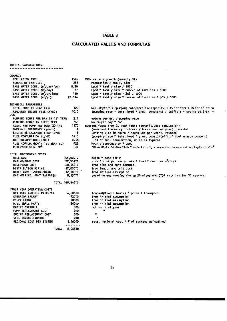
Table 3 also repeatsanother portion of Table 1—the derived costvaluesare shownalongwith formulas which show their derivation. Operatingcostsare shown for the first year ofsystem operation, which is one year after the project begins, to account for a one-yearconstruction period5.

The resultsof the newcostmodelcanbe compared with Reeser’s(beforeaccounting ratios).For 300 m well depth the investmentcostsare:

This analysis Reeser(1988)

Well 105,000Th 104,400ThEngine/Pump 27,955TD 21,000ThCMI Works 53,941TD 32,000ThOther 8,15OTD

Total 195,046Th 157,400Th

The new costsare often higher as they are basedon more recent, experienced-baseddata,and indude more costelements.6

~The assumption that operatingcosts (and benefits)begin in year 1 after an initial year of

construction is a revision of the model since the consultant’s trip to Tunisia In June-July1989

6 Thesewell costsuse a unit costof 350TD/meter,based on quotations for upcomingprojectwells (September 1989).

9

TABLE 1

OVERALL COST MODEL

DETAILED ASSUMPTIONS:

DEMAND:PDPULATION 1989POPULATION GROWTHRATE:FAMILY SIZEWATER CONSUMPTIONCLpcd):CONSUMPTIONGROWTHRATE:

TECHNICAL PARAMETERSTOTAL WELL DEPTH Cm):WELL STATIC WATERLEVEL(M)PUMPING RATE ([Is)SPECIFIC CAPACITY CL/s/H):DISTRIBUTION PIPING LENGTH Cm)RESERVOIR SIZE RATIOPUMP/ELECTRIC MOTOREFFICIENCYENGINE + GENERATOREFF1CIENCY

REGIONAL MAINT.CREW COST 174,000TD# OF SYSTEMSFOR PRORATING 150

FINANCIAL ASSUMPTIONSDISCOUNT RATEPROJECT PERIOD CYRS)

12.0%20

INITIAL CALCULATIONS:

DEMAND:POPULATION 1990NUMBEROF FAMILIESBASE WATERCONS. (m

3/day/fam)BASE WATER CONS. (m3/day)BASE WATERCONS. (m3/yr/farn)BASE WATERCONS. Cm3/yr)

TECHNICAL PARAMETERSTOTAL PUMPING HEAD Cm):REQUIRED ENGINE SIZE CKVA):PUMPING HOURS/DAY IN 1st YEARPUMPING HOURS IN FIRST YEARAVER. ANN PUMP. HRS OVER 2D YRSOVERHAULFREQUENCY(years)ENGINE REPLACEMENTFREQ.Cyrs)FUEL CONSUMPTIONCL/HR)OIL CONSUMPTIONCL/KR)FUEL CONSUM./HDNTH1st YEAR CL)RESERVOIR SIZE Cm3)

TOTAL INVESTMENT COSTSWELL COSTENGINE/PUMP COST

RESERVOIR COSTDISTRIBUTION PIPINGOTHER CIVIL WORKSCOSTSENGINEERING, GOVT SALARIES

FIRST YEAR OPERATING COSTS C199D)NET FUEL AND OIL PRICE/YROPERATORSALARYOTHER LABORMISC SMALL PARTSENGINE OVERHAULPUMP REPLACEMENTCOSTENGINE REPLACEMENTCOSTWELL RECONDITIONINGREGIONAL COST PER SYSTEM

1545258

0.3077

liD28,196

14240

2.1760

11704

1314.50.36

922SD

08-Aug-89

15003.0%

650

1.0%

300100

100.5

10000.5

54.9%17.4%

1503SOTD

2,204TD0.518

1.SOTD1 lTD

12, 000TD0.527

2563

0.291.2

3%10%10%

720TDSOOTD300TD

50002, 234TD

5 yrs15000 hrs

15,000TD11

INVESTMENT UNIT COSTSWELL COST PER m DEPTHENGINE COST/KVA - COEFFICIENTENGINE COST/KVA - EXPONENTPUMP COST PER m3/hr/mDISTRIBUTION PIPINGSTANDPOST, TROUGH, ETCRESERVOIR COST EXPONENTRESERVOIR COST COEFFICIENT

UNIT OPERATING COSTSFUEL PRICE (TOIL)OIL PRICE (TOIL)FUEL & OIL PR1CE ESCALATIONFUEL & OIL TRANSPORTCOSTSFUEL LOSS/WASTE/PILFERAGEOPERATORANNUAL SALARYOTHER IN-KIND ANNUAL LABORMISCELLANEOUSSMALL PARTSOVERHAULFREQUENCYCHRS)OVERHAULCOSTPUMP REPLACEMENTFREQUENCYENGINE REPLACEMENTFREQUENCYWELL RECONDITIONING COSTWELL RECONDITIONING IN YEAR

ACCOUNTINGRATIO

0.9131.0000.7250.725O.7251.000

0.8000.6500.6500.8500.8501.0001.0000.9000.825

SHADOWPRICE

95,813TD22 , 55 ‘I TO14 ,6O3TD12,325 10

8,700TD8, 15010

162, 14TTD

3,426TD468TD325TD255TD

OlDDTDDIDDTD

957TD

5,431TD

1D5,000TD22,55110

20,142TD17,0001012,ODDTD

8,15DTD

TOTAL 184,84310

4 ,283TD720TDSDOTD300TD

OTD010OTDOTD

1,16OTD

TOTAL 6,963TD

10

TABLE 2

INITIAL ASSUMPTIONS:

ASSUMPTIONSAND SOURCES

DEMAND:POPULATION 1989POPULATION GROWTHRATE:FAMILY SIZEWATERCONSUMPTIONClpd):CONSUMPTIONGROWTHRATE:

TECHNICAL PARAMETERSTOTAL WELL DEPTH Cm):STATIC WATERLEVEL Cm):PUMPING RATE (L/s)SPECIFIC CAPACITY (L/sfM)DISTRIBUTION PIPING LENGTHRESERVOIR SIZE RATIOPUMP/ELECTRIC MOTOREFFICIENCYENGINE + GENERATOREFFICIENCY

87%

INVESTMENT UNIT COSTSWELL COST PER m DEPTHENGINE COST/KVA-COEFFICIENTENGINE COST/KVA-EXPONENTPUMP COST PER n?/hr/mDISTRIBUTION PIPINGSTANDPOST, TROUGH, ETCRESERVOIR COST EXPONENTRESERVOIR COST COEFFICIENT

UNIT OPERATING COSTSFUEL PRICE CTD/L) 0.29OIL PRICE CTD/L) 1.2FUEL & OIL PRICE ESCALATION 3%FUEL & OIL TRANSPORTCOSTS 10%FUEL LOSS/WASTE/PILFERAGE 10%OPERATORANNUAL SALARY 720TDOTHER IN-KIND ANNUAL LABOR SOOTDMISCELLANEOUSSMALL PARTS 300TDOVERHAULFREQUENCYCHRS) 5000OVERHAULCOST 2,234TDPUMP REPLACEMENTFREQUENCYCyrs) 5ENGINE REPLACEMENTFREQ.Chrs) 15,000WELL RECONDITIONING IN YEAR 11REGIONAL MAINT.CREWCOST 174,000TD# OF SYSTEMSFOR PRORATING 150

FINANCIAL ASSUMPTIONSDISCOUNT RATEPROJECT PERIOD CYRS)

See Wyatt trip report in References.See Wyatt trip report in References.

15003.0%

6SO

1.0%

300100

100.5

10000.5

54.9%17.4%

350TD2,2D4TD

0.5181 .5OTD

1 7TD12,000TD

0.5272563TD

Typical value for project site, many different values used here.From Reeser, but comonly used by CTDA.Figure currently used by CTDA. Reeser used 7.5.Derived from Reeser’s 47 Lpcd. Also AUI uses 50.Estimated. AUI also uses 1%. Reeser had 0%

Typical value for project site, many different vaLues used here.In the absence of site-specific data, a value of 1/3 of welL depth used.Average used in 14 recent OOTC projects.In the absence of site-specific data, this valud, from ORE, is used.Average used in 14 recent ODTC projects.AUI design guideline. This gives size from mean daily consuiption.Estimated from local catalogs. Based on puip 67%, electric motor 82%.Estimated from local catalogs and field experience - engine 20%, generator -

In the absence of site specific data this estimate by CTDA and RSH used.Cost function derived from Local catalogs. See Wyatt trip report in References.Cost function derived from local catalogs. See Wyatt trip report in References.Estimated average cost in 14 recent ODTC projects.Average cost in 14 recent OOTC projects.Average cost in 14 recent OOTC projects.Cost function derived from Local catalogs.Cost function derived from local catalogs.

Current market price. Reeser had 0.27 in 1987, and 1988.Current market price. Reeser had 1.025 in 1987, and 1988Estimated. Reeser had 0%Based on conversations with operators. Reeser had same value.Estimated. Reeser had 0%Based on conversations with operators. Reeser had same value.Estimated In-kind contribution of coaninity menbers. Reeser had 0.Based on recent OOTC estimate. Reeser had 330.Estimate. Based on conversation with Local mechanics + engineers.15% of engine cost. Based on conversation with Local mechanics + engineers.Estimate. Based on conversation with Local mechanics + engineers.Estimate. Based on conversation with local mechanics + engineers.Based on discussion with ORE and CTDA staff

Based on discussion with ORE and CTDA staffBased on conversation with local officials.

Estimated from local interest rates. Reeser had 15% in ‘87, 10% in ‘88.Typical life of drilled wells.

12.0%20

11

DEMANO:POPULATION 1990NUMBEROF FAMILIESBASE WATER CONS. Cm~/day/fam)BASE WATERCONS. Cm3/day)BASE WATER CONS. Cm3/yr/fam)BASE WATERCONS. Cn?/yr)

TECHNICAL PARAMETERSTOTAL PIMPING HEAD Cm):REQUIRED ENGINE SIZE CKVA):

25%PUMPING HOURS PER DAY IN 1ST YEARPUMPING HOURS IN FIRST YEARAVER. ANN PUMP HRS OVER 20 YRSOVERHAULFREQUENCYCyears)ENGINE REPLACEMENTFREQ (yrs)FUEL CONSUMPTIONCL/HR)OIL CONSUMPTION(L/HR)FUEL CONSUM./MONTH1st YEAR CL)RESERVOIR SIZE Cm3)

TABLE 3

CALCULATED VALUES AND FORMULAS

1545258

0.3077

11028,196

12240.0

2.1765

11704

1314.50.3692250

TOTAL INVESTMENT COSTSWELL COSTENGINE/PUMP COSTRESERVOIR COSTDISTRIBUTION PIPINGOTHER CIVIL WORKSCOSTSENGINEERING, GOVT SALARIES

1O5,000TO22,551 TO20, 142T017,000TO12,000TO8, 150T0

TOTAL 169,843T0

depth * cost per msize * cost per kva + rate t head * cost per rn3/hr/M.from size and cost fornila.from length and unit costfrom initial assuiptlonbased on engineering fee on 20 sites and CTOA salaries for 30 systems.

FIRST YEAR OPERATING COSTSNET FUEL AND OIL PRICE/YROPERATORSALARYOTHER LABORMISC SMALL PARTSENGINE OVERHAULPUMP REPLACEMENTCOSTENGINE REPLACEMENTCOSTWELL RECONDITIONINGREGIONAL COST PER SYSTEM

4, 283TO72OT0500TD300TO

OTOOTOOTOOTD

1,160T0

TOTAL 6,963TO

(consuiption + waste) * price + transportfrom initial assuiptionfrom initial assuiptionfrom initial assuiptionnot in first year

‘I

H

I’

total regional cost / # of systems maintained

INITIAL CALCULATIONS:

1989 vaLue + growth (usually 3%)Population / family sizeLpcd * family size / 1000Lpcd • family size * nuiter of families / 1000Lpcd * family size * 365 / 1000Lpcd * family size * nuiter of families * 365 / 1000

Well depth/3 + Cpuiping rate/specific capacity) + 15 for tank + 5% for friction(puiping rate * total head * gray, constant] / Ceffic’s * cosine (0.8)]) +

volune per day / puiping ratehours per day * 365

average found from 20 year table (Benefit/Cost tabulation)

(overhaul frequency in hours / hours use per year), rounded(engine life In hours / hours use per year), rounded(pulping rate * total head * gray. const)/Ceffic.* fueL energy content)2.5% of fuel consurption, which is typical.hourly consuiption * use.(mean daily consuiption * size ratio), rounded up to nearest moltiple of 25m3

12

Thenewmodel assumesaccountingratiosto calculateshadowpricesfrom marketvalues,asdid Reeser.While availabledataare limited, severaleconomicstudieswerecollectedaridreviewed. The table below showsassumedaccountingratios for labor and commoditycategories.ThereIs little variationamongsourcesfor someitems, but a wide variationforothers.For example,dieselfuel variedfrom 1.38, In a 1984World Bank Irrigation projectappraisalreport, to 0.60 (for dieselenergy)in the 1987 SCETirrigation studies. Thehighvaluein the World Bank reportwaschosenbecauseof high subsidieswhich werein placeat the time. These subsidies have been lifted, so more recent estimatesare lower.Nonetheless,reliablecurrentestimatesfor theseaccountingratiosarenot available. Sothebestpossibleestimatewasmadebasedon thesedataandspecificanecdotalInformationonthedifferentcommodities. This analysisusesthesebestestimatesin thetable below.

In Chapter6, sensitivIty of themodel to theseaccountingratiosis explained. In general,thesensitivityis low. However,themodel is rathersensitiveto theaccountingratiofor unskilledlabor, asthis is applied to the total project benefits. As can be seenin the table, thevariationamongsourcesis low for this parameter.

Source ValuesUsed InWorld Bank Reeser SCET AIRD This Analysis

(1984) (1987) (1987) (1987)

General

Unskilled Labor 0 75 065 0.65 — 065Semiskilledlabor — 0 82 — 086 O~825Skilled Labor 0 80 1.00 1 00 — 1 00Local Materials 0 80Imported MaterIals 100

Specific

Well Drilling — 0 85 0 909 0.9131Civil Works 0 54 0 77 0.955 0.7252DieselFuel, 011 1 38 0 70 (060) 098 0.80~SmallParts 0.63 085 — 0.75 0 85~Overhauls — — — 085~Pumps, EngInes 0 77 0~85 068 1 006

MaintenanceLabor 0 825~70 hp Tractor 0 77 097 097 0.94 —

Well reconditioning — — — — 0 90~

NOTES

1 1/2 ImportedMaterials+ 1/2 SemiskIlledLabor — (1+ 825)/2 — 0.9132 1/2 Local Materials+ 1/2 Unskilled Labor3 Local Material4 3/4 Local Material + 1/4 ImportedMaterial5 3/4 Local Material + 1/4 ImportedMaterial6 ImportedMaterial7 SemiskIlled labor8 1/2 Local Material + 1/2 SkIlled Labor

13

Box 2

KEY DIFFERENCESBETWEEN THE IDA MODELAND THE NEW COSTMODEL

• Reeserusedolder costdata,not basedon experiencewith the currenttype of project.Real historicaldataare usedbere.

• Reeserdid not accountfor the causallink betweendepth,pumpingrate,and fuel conswnption.This analysisusesrelevantengineeringfomuilas.

• Reeserdid notincludeoverhaulcosts,costsof regional supportcrews,engineeiing,and goveriineniagents’salaries,all of which are directly liuked to the establishmentand O&M of thesesystemsandare includedhere.

14

Chapter 5

BENEFIT CALCULATIONS

5.1 IDA Approach

Reeser’scalculationof benefitsof rural waterprojectsis basedon timesavingsfor usersandan estimateof the economicvalueof time. Heassumes,logically, that creationof a waterpoint will savetime for thefamiliesnearbyby reducingthe distancetheyhaveto travel.

Reeserestimatesthe time savingsfrom datacollectedby Smith, in a rural survey of 40families, In 1985.ThoseresultsIndicatedthattheaveragefamily spendsabout60 hoursperweekcollectingwater.Reeserassumesthenewprojectwill savehalf of this time, but givesno basisfor thisassumption.Thetimespenton collectingwaterwasestimatedas37 percentby men,39 percentby women,and29percentby children.Reeserassumesthatthebenefitof thewaterprojectwill be thatmenwon’t haveto go for waterany more;womencannowdo it becausethewell Is doser.Social conventiondictatesthata womanmaynot travel witha donkeycartto a distantwell. Sothebenefitscan be foundfrom the earnIngpowerof themen who no longer haveto haul water. He usesthe local minimum wage at the time(O.362TD),multiplied by the employmentrate(72 percent),multiplied by the accountingratio for unskilled labor(65 percent)to estimatethevalueof themen’s time.

To review:

Benefits 60 hrs/wk • 50% ~vlngs • 37%men • 0.362 iD/hr • 72%emp). 52 weeks• 65%economIcvalue

= 577 his/~rr 0.26 1 TI) 65% (accowitkig ratio)

97 TD / family / war.

Reeserusedthis value for all peopleliving withIn 4 km of a new waterpoint. He alsoassumedpeoplelMng from 4 to 7 km would getfewerbenefits,beingfurtheraway,anduseda valueof 20Th per family peryear,or one-fifth of thebenefitsfor thecloserresidents,forthem.

Thereareseveralquestionableaspectsto this calculation.First of all, the figureof 60hoursperweek seemshigh. The consultant’sexperiencefrom visiting more than 10 villages InCentralTunisia anddiscussingtheseissueswith countlesspeople(in February1989)Is thaton averagepeopledon’tspendanywherenearthisamountof time.Peoplewith donkeycartsof 500liter capacitywon’ttravel thatmuch.Perhapsthedifference betweenthis finding andSmith’sis dueto themore widespreaduseof donkeycartswhich hasbeenpromotedby the

15

governmentIn thepastseveralyears.Unfortunately,little Is knownabouthoworfrom whomSmithcollectedthereportednumbers.

Secondly,the assumptionthat the benefitsderive only from time savingsby men seemswrongandshort-sighted.Men,women,andchildrenall participatein thecollectionof water,andwomenaregenerallybelievedto play a majorif not predominantrole In the collectionanduseof water.Their role maybe much moredominantIn theusethanIn the collectionandtransportof water. It Is true,however,that a long trip to adistantwell Is morelikely tobe the job of a man.If menareliberatedfrom this taskbecausethewaterIs closer,theydo,in theory,havetheopportunityto earnmore money.But thewomenor childrenstill haveto collectthewater. In facttheymayhavea newburden.Their time certainlyhasa valueaswell. At presentthereareInsufficient recentreliabledataon who collectswater,distancestraveled,mode of transport,and time spent.Despitethe inability to be preciseon theseissues,themostimportantpoint in the benefitcalculationremainsthatthe distancetraveledwill be less, no matterwho Is going for water,how, or for whatpurpose.

5.2 The RevisedApproach

A truebenefitscalculationwould be basedon the changeIn consumersurplusasa resultofthe project. This typeof calculationwould haveto be basedon currentandfuture priceofwater,be it pricein currencyor In time to collect it, anda demandfunction, relatingpriceand consumption. Separatedemandinformation might be neededfor drinking water,livestock watering,and small Irrigation. Unfortunatelysuchdemanddataare simply notavailablefor ruralTunisia.Theestimationof thesedemanddatarequiresamajorfield study.

In orderto makesomeimprovementsin thecomputationof benefits,arevisedapproachwasdevelopedbasedon the limited dataavailable currently. This approachusestravel timesavingsasthebasicbenefit. In additIon,theapproachusesanempiricalestimateof thevalueof time, derivedfrom theoverall behaviorof the rural populationin theregion.This valueof time is Independentof the persontravelingandof theintendeduseof water.

ProjectRadiusandDistanceSavings

The computationof travel distancesavings must be basedon a definition of the traveldistancebeforeandafterthesitewatersupplyproject.While investigatinga locationasasitefor a watersystem,CTDA staff visit the areaanddeterminewherethe populationusuallygoesfor water.Typically this Involves travel to awell, which might be6, 8, 10 or even 12km away. Somevillagersmay travel themselves,andsomewill buy from vendorswhomakethetrip. This representstheone-waytravel distancebeforetheproject.

The travel distanceafter the project can be establishedin severalways. One approach,consistentwith thelong-termnorm of the Ministry of Plan,would be to a~imeeveryone

16

within a 3 km radiusIs a beneficiary,andthat the averagetravel distanceafterthe projectwould be 1.5 km (oneway),which assumesthatthe populationdensityis uniformwithin that3 km radius. Reeserdid somethinglike that but used4 km, andassumedthat peopleasfaras7 km awaywould alsobenefit to a lesserdegree.

Discussionswith CTDA staff led to anotherapproach.It seemedmostlogical to think of aprojectradius,not of 3 km but of a distanceequalto one-halfthe distanceto the closestexisting well. For example,a sitewith an existing well 10 km awaywould havea projectradiusof 5 km. Anyonewholived 6 km awayfrom thesitewould tendto go to theexistingwell, rather thanthe new one, evenafter the new one was built. Then the new traveldistancewould be equalto one-halfthe projectradius,or 2.5 km for theexampleabove.Intheend,theaveragetravel distancesavingswould be,by simplemathematics,three-fourthsof the distanceto theexisting well.

This approacharguesthat peopleat very isolatedsiteswould tendto havemoredistancesavingsthan thosenot very far from an existing source.This logical effect is certainlyanimprovementover Reeser’suniform useof 4 km and 7 km. It wasrecognizedthat suchacalculationIs still approximatebecause,in reality, populationsareriot uniformly distributed,andwells arenotevenlyspacedarounda topographicallyuniform countryside.Trying to beany moreprecisewould forcethemethodto be totally site-specific,which wasundesirablein suchan analysis.Thisapproachdoesrepresenta morerealisticandlogical modelof thesesmall waterprojectsand theway peoplebehave.

The populationservedby the project must be computedIn relation to the project radius.CTDA staff typically collectpopulationdatawithin aradiusof 3 km and6 km. If theprojectradiusis 4 krn, anestimatedbeneficiarypopulationcanbe foundby addingthe populationwithin 3 km andaproratedportionof thepopulationbetween3 and6 km, asshownIn Box3 below.

Time SavingsThe time savingscan be directly computedfrom distancesavings,the averagespeedoftravel, andthenumberof trips takenperyear(which in turndependson thewaterconsumedandthetransportcapacity),asdescribedIn Box 4 below. Thesecalculationsweremadeforthepeoplewho usedonkeycarts.

17

POPULATION COMPUTATION

Box 3

Value of Time

Theav~raqevalueof time for waterusersin rural CentralTunisia canbeestimatedfrom theircurrent overall behavior. The choice peoplemust make In obtaining water is betweenspendingtime In thedonkeycartandbuyingwaterfrom vendors.Knowledgeaboutpeople’sbehaviorwhenfacedwith this choice(time or money)leadsto an estimateof the valueoftime. Local villagersandgovernmentofficials estimatethat currentlyabout 50 percentbuytheir water from vendorsand 50 percentuse500 liter donkeycarts. If half chooseoneoptionaridhalf choosethe other, it could besaidthat the averagefamily Is indifferentto thetwo options.Thuswecanwrite an equationequatingthe costof the two options,asshownin Box 5. This notion that behaviorcan lead to an assessmentof the value of time isfundamentalto this approachand is derived from field work by Whlttlngton, et al. (seeReferences).

Populationfor a Population Land Area Population DensItyPro~ectRadlusofR- lnskie3km + from3~>R • ofarea3->6krnwhen 3 <R < 6

This assumesthatthepopulationdensityIn the area from 3km to R is the sameas thepopulation density from 3 to 6 km, which will not always be accurate,but seemsreasonable.Algebraicsimpilficatlonsleadsto:

PopulationforProject Radius of Rwhen3 < R < 6

(P3x(62-R2))-i-IP

6x(R2-32)j

(62 32)

where:P

3 — PopulationwIthin 3 kmP6 — PopulationwIthin 6 km

18

TIME SAVINGS COMPUTATION

Time Savings/Family/Yr — Time Savlngsflrlp Trips/Family/Yr

where~

2 x (D1 - D2)

S C

P x Q x 365

D — Distanceto closestexisting sourceof water, kmD1 — Travel distancebeforeproject, km — DD2 — Travel distanceafter project, km — (D/2)/2 — D/4S — Travelspeed,km/hr - (A valueof 5 km/hr wasgenerallyused)P — Peopleper family - (A value of 6 wasgenerallyused)Q — Water use,Vperson/day- (50 Vp/d wasgenerallyused)C — Cartwatercapacity- (A valueof 5001 wasgenerallyused)

Combining the simplifications andassumedvaluesabove, the result is:

2x(D-D/4) 6x50x365Time Savings,Pamlhj/Yr- - * ______

5 500

— 65.7 D, in hours/family/year

@D- 4km@D- 6km@D- 8km@D- 10km

— 263hours/yearor 5.0 hours/week— 394hours/yearor 7.6 hours/week— 526hours/year or 10.1 hours/week— 657 hours/yearor 12.6hours/week

Note that thesesavings are far less than the valuesused t~*jReeser(30 hrs/weekor 1560hours/yr).Howeverif Reeser’svalueof 37% male labor isappliedthe “valued”time savingsfallsto 577hrs/yr or 11.1 hrs/week,which is similar to the valuesabove.

It Is also Importantto realize that if only 40 1/trip arecarried,as would be the caseof a personwalldng with a donkey,the resultsarevery muchhigher. Thus the quantity hauledis a veryimportantvariable.

Box 4

19

VALUE OF TIME ESTIMA11ON

MEANS OFOBTAiNINGWATER:

BUYING FROM VENDORS or USING DONKEY CART

COST OFOBTAINiNGWATER

Price of waterpaid to vendor

r 1 r 1lValue- I ITravel

— of-time VITIme 1+L .J L J

r 1I Priceof water

I paldatwell IL

By re-arrangingwe obtain:

Given that

Value-of-timePriceof waterpaid to vendor- Price of waterpaid at well

(Travel Time)

VendorPrice(ID) - (2 + 0.75x D) for 3.5 m3 of water.

0.571 + 0.214D , In TD/ni3

whereD — distancetraveled(oneway)

Note: this formula Is basedon informal surveysIn severalcommunitiesIn theCTDA areaIn February1989.

Price at Well (TD) — 0.100TD for 0.5m3 0.200 TD/m3

Trave1Time~hrs/m3)=(2 D/S)/C

where:S - Travelspeed,km,lir - (5 km/br)C -Cartwatercapedty-(0.5m3)

The following resultsareobtained:

Note that the value-of-timedoesnot dependheavily on the travel distance.For benefit calculationsthevalue-of-time@ 6 kin was used,asthis distanceseemsthe best overall estimateof the “average”traveldistancefor the Kasserine/Gaf~ruralpopulation.Note that the currentminhm.x~agiiculturalwageIs0.400TD, Indicatingthat theabovevaluesof timeare rather high

Box 5

D3km6km9km

Value-of-time -

0.423TD ~.

0.345ID0.320ID

20

Benefit Calculations

An overall assessmentof benefitscanbeobtainedby multiplying theestimatedaveragevalueof time by the travel time savingsper family per year. Box 6 shows the results. Theeconomicvalueof thesebenefitswasfoundby multiplying thedirect benefitsby theassumedaccountingratio for unskilled labor (0.65, asdiscussedIn Chapter4). Theseresultscanbemultiplied by the numberof families in the project radiusto get total project benefits.

Box 6

The valuesof benefitsper family per year are somewhat higher than thosecalculatedbyReeser,who estimated98Th for peopleup to 4 km away, and 20Th for people out to 7km. The difference betweenReeser’sresultsand theseIs mostly due to higher value of timein this analysis.

There are a number of aspectsof this benefit calculation which must be discussed.First ofall, valueof time wasestimatedfrom behavior of the group as a whole, andthus is usedtocomputebenefitsfor the group, that is, the averagevalueof time Is usedto get the averagefamily benefits.It Is very likely that many families will havea higher valueof time, and othersmuchlower. But thereare insufficient data to estimatethesevariations,andaveragevaluesmust beused.

Secondly,the benefitscould be computeddifferently—by addingthe cashsavingsof thosewho buy from vendorsand the valueof travel time savingsof those who do not. Truefinancial benefitsto familieswho usevendorscould be computedby estimatingthe drop invendor pricesdue to decreasedtravel distance,usingthe simple price fonTlula shown in Box5. There doesappearto be sufficient competitionamongvendorsso that decreasedtraveldistanceswill leadto cashsavingsfor the buyers.However,the calculationof the valueoftravel time savingsfor thosewho do not buy from vendorsbecomesdifficult. Thesepeoplewill havea valueof timedifferent from our global estimate(probablylower). In fact, there areno data uponwhich to estimatethe valueof time for thesepeople.Thus it appearsbetterto computebenefitsfor all families basedon traveltie savings,using theoneavailable valueof time estimate.

BENEFITS COMPtTrATION

1mw! Tsavel EconomkDlstar,ce Profact Dl~ance Dl~ar,ce Time Savings Valus- Benefitsper BenefitsperBefore Radius After Savings perfamily/yr of-Time farralyper yr faMh~,per yr

4km 2km 1.0km 3.0km 263 hrs 0.345T0 91TD 59TD6 3 1.5 4.5 394 0.345 136 888 4 2.0 6.0 525 0.345 182 11810 5 2.5 7.5 657 0.345 227 14812 6 3.0 10.0 788 0.345 272 177

21

Thirdly, thIs approach,becauseit is basedon people’s behavior,reflects people’sownvaluationof benefits.It assesses,althoughwith only limited data, what familiesare willing topay (In time or cash) for water—whichhelps estimatethe value they place on It. Thiscomputationof benefitsdoesnot assumepeople are using the water for any particularpurpose,so it makesno Inferencesaboutbenefitsassociatedwith use.For example,nograndassumptionsare madeon the Improved condition of livestockin thearea,orincreasedfamily revenueor nutrition from Irrigationwater.People’sbehaviorpermitsthemeasurementof their own assessmentof all thesebenefits. Nor does this computation makeanyassumptionsabout what peoplemightdo in thefree time theyhavenow thatwater is closer.It could be stated,however,that rural peopledo riot fully appreciate the potential healthbenefitsfrom largerquantitiesof deanerwater,and that thesebenefitsare not counted. Thisis probably true, but the quantitativeassessmentof thesebenefitsIsvery difficult.

Fourthly, this approachassumesthat people’sconsumptionofwater is basicallyinelastic, thatis, it assumesthatpeoplewill consumethe sameamountof water(50 lpcd) beforeandaftertheproject. This is probablynot true, althoughtheextentof the increasein consumptioncould be small for somefamiliesandlargefor others,andmaychangeover time. A generalIncreaseof 1 percentin percapitawaterconsumptionperyearis assumedto try to addressthis issue.

A much better assessmentof project benefits is possible,given the upcomingfield researchplannedfor the project. Suchfield datacollection should assessthe behavior of differenttypes of water users beforeand after the Installationof water systemsin severalvillages.Surveys should collect data from randomly selected families in selectedcommunities.Questionsshouldexaminebehavior(wateruse,time spent,cashspent,persontraveling)forfamilieswho beforetheprojectwalkedfor water,whowent In donkeycarts,or who boughtfrom vendors.Familieswho usetwo or threeof thesecollection methodsshould also besurveyed. Additional dataon income,occupations,family size, education level, and basichealthconditionsshould alsobe collectedat thesametime, for correlationwith waterusepatterns.SurveysshouldbeconductedbeforearidafterwatersystemsareInstalled,allowingquantitativeassessmentof behavioraland consumptionchanges,aswell as cashor timesavings,leadingto betterestimatesof benefits.

22

Chapter 6

RESULTS

6.1 Comparisonof BenefitsandCosts

Costsand benefitswerecombinedin a Lotus 123worksheet,usinga 20-yearprojectperiod.A discountrate of 12 percentwas used, based on current bank lending rates. InitialInvestmentsare assumedto occurIn yearzero, during construction.Benefitsarid operatingcostsare assumedto start in the first year,andcontinuethroughthe twentieth year.Tables4, 5, 6 and Figure 1 show inputs andresultsfor a hypotheticalexampleof 1,500 peoplewithin a project radius of 4 km, with a previous travel distanceof 8 km and an estimatedwelldepth of 300 rn Resultsshow a B/C ratio of 1.25andan IRR of 16.7 percent.

23

Table 4

BASiC INPUT OUTPUTCOMPUTERSCREEN

CTDA USAID/TUNISIA RURAL POTABLE WATERINSTITUTIONS PROJECT No. 664 0337

PROJECT SITE ECONOMICANALYSIS

INPUTS: RESULTS:

20-Feb-90

SITE:DELEGATION:COUVER.NORAT:POPULATION 3 KM 1989:POPULATION 6 KM 1989:ORIG. TRAVEL DIST.(km)PROJECTRADIUS(kin):POPULATION SERVED 1989POP. GROWTHRATE:TOTAL WELL DEPTH(rn):STATIC WATERLEVEL (in)PUMPINGRATE (us):DISTRIB. LENGTH (to):

DISCOUNT RATE:ESTIMATED WELL COST/rn

INITIAL FIN. INVESTMENTINITIAL INVEST/PERSONTOTAL ECON. PV COSTTOTAL ECON COST/PERSONTOTAL ECON. COST/rn3AVERAGEOPER. FIRS / YRAVERAGEANN. O&M COSTCOMNIJN. CONTRIB. TO O&MTIME SAVINGS/FAX/YRECONBENEFIT/FAM/ist YRTOTAL ECON. PV BENEFITSNET PRESENTVALUEBENEFITS / COSTSIRR

176, 693TD118TD

234,884TD157TD

0.279TD1170

12,O6OTD7,720TD

526118TD

293,809TD58, 925TD

1.2516.7%

SAMPLE

15001500

84

15003.0%300100

101000

12%350TD

24

Table 5

INITIAL BENEFIT AND COST CALCULATIONS

DETAILED ASSUMPTIONS:

DEMAND:POPULATION 1989POPULATION GROWTHRATE:FAMILY SIZEWATERCONSUMPTION CLpd):CONSUMPTIONGROWTHRATE:

TECHNICAL PARAMETERSTOTAL WELL DEPTH Cm):WELL STATIC WATER LEVEL(M)PUMPING RATE (L/s)SPECIFIC CAPACITY CL/s/M):DISTRIBUTION PIPING LENGTH CRESERVOIR SIZE RATIOPUMP/ELECTRIC MOTOR EFFICIENENGINE + GENERATOREFFICIENC

REGIONAL MAINT.CREW COST 174,000TD# OF SYSTEMSFOR PRORATING 150

INITIAL CALCULATIONS:

DEMAND:POPULATION 1990NUMBEROF FAMILIESBASE WATERCONS. (n?/day/fam)BASE WATERCONS. Cr1

13/day)BASE WATER CONS. Cm3/yr/fam)BASE WATER CONS. Cm3/yr)

TECHNICAL PARAMETERSTOTAL PUMPING HEAD Cm):REQUIRED ENGINE SIZE CKVA):PUMPING HOURS/DAY IN 1st YEARPUMPING HOURS IN FIRST YEARAVER. ANN PUMP. MRS OVER 20 YRSOVERHAULFREQUENCYCycars)ENGINE REPLACEMENTFREQ.(yrs)FUEL CONSUMPTIONCL/HR)OIL CONSUMPTIONCL/HR)FUEL CONSUM./MONTH1st YEAR CL)RESERVOIR SIZE Cm3)

TOTAL INVESTMENT COSTSWELL COSTENGINE/PUMP COST

RESERVOIR COSTDISTRIBUTION PIPINGOTHER CIVIL WORKSCOSTSENGINEERING, GOVT SALARIES

FIRST YEAR OPERATING COSTS C1990)NET FUEL AND OIL PRICE/YROPERATOR SALARYOTHER LABORMISC SMALL PARTSENGINE OVERHAULPUMP REPLACEMENTCOSTENGINE REPLACEMENTCOSTWELL RECONDITIONINGREGIONAL COST PER SYSTEM

1545258

0.3077

11028,196

14240

2.1760

11704

1314.50.36

92250

FINANCIAL ASSUMPTIONSDISCOUNT RATEPROJECT PERIOD CYRS)

0.650 118TD0.650 30,35010

15003.0%

650

1.0%

300100

100.5

10000.5

54.9%17.4%

350TD2,204TD

0.5181.5OTD

1 7TD12, 000TD

0.5272563

0.291.2

3%10%10%

720TD500TD300TD5000

2,234TD5 yrs

15000 hrs15,000TD

11

INVESTMENT UNIT COSTSWELL COST PER m DEPTHENGINE COST/KVA - COEFFICIENENGINE COST/KVA - EXPONENTPUMP COST PER m3/hr/mDISTRIBUTION PIPINGSTANDPOST, TROUGH, ETCRESERVOIR COST EXPONENTRESERVOIR COST COEFFICIENT

UNIT OPERATING COSTSFUEL PRICE CTD/L)OIL PRICE CTD/L)FUEL & OIL PRICE ESCALATIONFUEL & OIL TRANSPORTCOSTSFUEL LOSS/WASTE/PILFERAGEOPERATORANNUAL SALARYOTHER IN-KIND ANNUAL LABORMISCELLANEOUSSMALL PARTSOVERHAUL FREQUENCY CHRS)OVERHAULCOSTPUMP REPLACEMENTFREQUENCYENGINE REPLACEMENTFREQUENCYWELL RECONDITIONING COSTWELL RECONDITIONING IN YEAR

ACCOUNTINGRATIO

0.9131,0000.7250.7250.7251.000

0.8000.6500.6500.8500.8501.0001.0000.9000.825

SHADOWPRICE

95,8131022,551T014,6031012, 325 TO8,700108, 15010

162, 141TD

3,4261046810325TO255 TO

OTD010OTD010

957T0

105,000TD22,551TD

20, 142TD17,000TD12,000TD8,15OTD

TOTAL 184,843TD

4, 283TD72OTD500TD300TD

OTDOTDOTDOTD

1,16OTD

12.0%20

PARAMETERSFOR BENEFIT CALCULATIONPREVIOUS MEAN TRAVEL DISTANCE 8NEW MEAN TRAVEL DISTANCE Ckm 2DONKEYCART CAPACITY CL) 500DONKEYCART TRAVEL SPEED CKM 5VALUE OF TIME CTD/HR) O.34STD

TOTAL 6,963TD 5,43110

BENEFIT CALCULATIONSAVINGS TRAVEL DISTANCE Cl way)DAYS BETWEENTRIPS 1st YEARTRIPS PER YEAR 1st YEARTOTAL TRAVEL SAVEO/FAMILY(km/yrTIME SAVINGS/FAMILY Chrs/yr)TIME SAVINGS/FAMILY/WEEK Chrs)ANNUAL BENEFITS/FfrMILY 1st YEARTOTAL BASE YEAR BENEFITS

61.67

2192628

52610.1

181TD46,693TD

25

SEREPIT / COST TARULATION SAWLE SITE

21-Feb-90

Table 6

20 YEAR TABULATION OF BENEFITS AND COSTS

wallOthat

Total 162141

OPERATING COSTS, TOFual, Trnport, OILOperator, Other LaborMIsc Salt PartsO’eerhaulafllel I Reconclltl~jor ReptaceantsReilonat Nalntan. Craw

Total

01$ COSTS PER .3

TOTAl. AIIIJA1. COSTSDIIWUTEO COSTS

o 3426 3671 3934 4215 451? 4840 5186 5557 5954 6380 6836 7325 7848 8410 9011 9655 10346 11086 1)878 127210 793 793 793 793 793 793 793 793 793 793 793 793 793 793 793 793 793 793 793 7930 255 255 255 255 255 255 255 255 255 255 255 255 255 255 255 255 255 255 255 255O 0 0 0 1699 0 0 1699 0 0135001699 0 0 0 1699 0 0 0 len

0 0 0 0 0 5103 0 0 0 0 5103 0 0 14396 0 5103 0 0 0 0 51130 95? 957 957 957 95? 957 95? 957 957 95? 95? 95? 957 957 957 957 957 957 957 957

O 5431 5676 5939 6119 11625 6845 7191 9461 7959 13488 22341 11229 24750 10415 16119 13560 12351 13091 13863 21735O 0.185 0.186 0.167 0.246 0.336 0.192 0.193 0.245 0.196 0.322 0.513 0.248 0.525 0.212 0.316 0.256 0.224 0.226 0.232 0.350

162141 5431 5676 5939 6119 11625 6845 7191 9461 7959 13488 22341 11229 24750 10415 16119 13560 12351 13091 13883 21735162141 4649 4525 4227 5160 6596 3468 3253 3821 2670 4343 6422 2882 5672 2131 2945 2212 1799 1702 1612 2253

PRESENT VALUE Of COSTSPY OP COSTS PER PERSONPV COST PER .3

234884157

0.279

RE1EF ITS

M~flEROP PAIR ITSNEFITS PER FMIILT

TOIA1. IE1IEFITSDI~STE0 RENEFI’TS

250 258 265 273 201 290 299 307 317 326 336 346 356 367 378 389 401 413 626 436 4520 116 119 120 121 123 124 125 126 128 129 130 131 133 134 135 137 138 140 141 142O 30350 31574 32846 34170 35547 36979 38470 40020 41633 43310 45056 46872 48761 50726 52770 54896 57109 59410 61804 64295O 27099 25170 23379 21715 20170 18735 17402 16163 15013 13945 12952 12031 11175 10379 9641 8955 8318 7726 7176 6665

P11*117 VALUE Of RENEFITS 293809

PV OP RENEFITS PER PERSON 196PY UFITR PER .3 0.349

UPITI I COSTS 1.25NET PRESENT VALUE 58925NPV PER PERSON 39

RET ECONONIC “CASN FL(1J” -162141 24919 25897 26907 26050 23922 30135 31279 30559 33674 29823 22715 35643 24011 40311 36651 41337 44758 46320 47921 42560INTERNAL RATE Of RETURN 16.7%

CIJRAATIVE COST (000 01)OJAILATIVE RENEFIT (0000T)QUIJLATIVE SPY (000 OT)

162 167 172 176 181 187 191 194 198 201 205 212 215 220 222 225 228 229 231 233 2350 27 52 76 97 III 136 154 170 185 199 2*2 224 235 245 255 264 272 280 287 294

-162 -140 -119 -100 -84 -70 -55 -41 -26 -16 -6 0 9 15 23 30 36 43 49 55 59

PROJECTTEAR 0 I 2 3 4 5 6 7 8 9 10 11 12 13 14 IS 16 17 18 19 60TEAR 1969 1990 1991 1992 1993 1994 1995 1996 1997 1998 1999 2000 2001 2002 2003 2004 2005 2006 200? 2006 2109POPULATION 1500 1545 1591 1639 1688 1739 1791 1845 1900 1957 2016 2076 2139 2203 2269 2337 2407 2479 2554 2630 2709~TER OEIMIIO (.3/day) 77 80 84 87 90 94 98 102 106 110 115 119 124 129 134 140 145 151 IS? 164 IllPIING N~MSper day 2.1 2.2 2.3 2.4 2.5 2.6 2.7 2.8 2.9 3.1 3.2 3.3 3.4 3.6 3.7 3.9 4.0 4.2 4.4 4.5 4.7

I~STI�RTCOSTS, TO95813 0 0 0 0 0 0 0 0 0 0 0 0 0 0 0 0 0 0 0 I66329 0 0 0 0 0 0 0 0 0 0 0 0 0 0 0 0 0 0 o .

0 0 0 0 0 0 0 0 0 0 0 0 0 0 0 0 0 0 0 •

a’

COSTS. RENEflTS CThouIand. of To)ECONOMIC COST. DICThou.oncS!)

z azC

U.—

C!) ~o.‘1

TiI— r,A nfll rzi -n -In >> C

— z—1 c -.

r -.N)a

~

zzC

noWU’

20.-. rU,

211)

~rn0C

Sa

N) N) P.) P.S0 t~ a a a o P.) a a. a o a 0.

-. N) u a0 0 0 0 0

La a. -j a w 0 - N) u a U’ o~ -j a0 0 0 0 0 0 0 0 0 0 0 0 0 0

I,,,,.. I I I I

n ‘f/f//f/n

~f/f//f/A

1//f/f//fl

1//f//f//A

“f//f//tn

‘ft/////i~/zA

~/////tff/t//f/A

czL’fl,A.flflfl,flfld,JN) -0 __________

The resultsfrom this newmodelandReeser’sresultsare comparedin Box 7. (Detailsof theresultsare given in AppendixC.) To be consistent,severalof Reeser’sInputs were usedasinputshere—forexample,discountrate(10 percent),populations(seeBox 7), anddrillingcosts(seeBox 7)1• It is clearthat thenewanalysisyieldsconsistentlyhigherIRRs, indicatingthe economicfeasibility of theseprojectsis much higher than Initially calculated. Thisdifferencecanbeattributedmostly to increasedbenefits,In turn dueto theincreasedvalueof time.

Box 7

6.2 Results—ModelSensitivity

An analysissuchasthis will be sensitiveto theInput parametersto someextent.A modelcanbe saidto be sensitiveto a particularvariableIf a moderatechangeIn thevariableleadsto a largechangeIn theresults.Ideally, sensitiveparametersshouldbeidentified, andcarefuldeterminationmadeof input data for thesevariables.

Someparametersare site-specific,such as well depth, population,and distancetraveled.Other parametersshould be consideredInternal to the model, suchasdiscountrate,valueof time, or accountingratios.Still other variableswill be well-definedand subject to little

‘Ree.erderivedhis populationestimatesfrom the WaterResourcesMapping Study Maps.After Rnea~ccuçletedhis study inFeb. 1988, fIeld wotk wasconductedby OTDC on actual populteionaaroundmostof tbeacsites.Most hadhigherpopelationsthanReeser’sestimates,so currenteconomicswill bedifferent.

SITE

COMPARISON OF ECONOMIC ANALYSES

ASSUMED ASSUMEDPOPULATION WELL COST

REESERll~R

THIS ANALYSIS

BiadhaZannoucheEl JadidaOuled ZidOuledBoullalegueKodiat TrichaSergLahmarToulabiaBrahim Zahhar

OWedAhmed

110417529383334391393956814

23152181

525 TD/m439362398362348348348348348

3.6%8.6%

-0.5%-7.4%-7.0%4.9%0.9%1.4%

11.5%16.7%

12.4%20.1%5.7%

-3.8%-3.7%13.3%7.8%9.1%231%32.3%

1.161.590.800.400.411.190.890.971.682.24

Note In o,der to compere to Reeser’s results, the new model wm computed using 10% dIscountrete,and using eproj~tradius of 4km (old beveldlstenceof 8 lcm), for nfl sites

28

variation,such asthe diesel fuel price, or the costof piping. Model sensitivity to site-specific

parametersIs not of much concern, as such parametersare so fundamental to a project thatfield survey datawill be collected and entered Into the model. Similarly, sensitivityto variableswhich changelittle maybe interesting but not of much consequence. But if the model is

highly sensitiveto internal or poorly defined parameters like value of time or discountrate,

this fact must be recognized and resultsusedwith a comprehension of the sensitivity to the

assumedvalues.

A full sensitivityanalysiswasnotcarriedout for lackof time. However,sensitivity to selectedkey parameters,including population, well depth, original distancetraveled,discountrate,water use(lpcd), valueof time, andpumping rate, wasstudied.

Using the basecaseof 1,500 people,8 km old travel distance,and 300 m well depth, andresultsof a B/C ratio of 1.25andan IRR of 16.7 percent, the sensitivityof the model canbe gauged.Box 8 showsB/C and IRR valuesfor alternativeassumptions.

Sensitivitycanalsobe examinedby calculatinglargetablesofresultsfor multiple input values.Sensitivity to population,well depth, and travel distanceIs given in Tables 8, 9, and 10.Sensitivity to the other parametersis shown In Appendix B. Sensitivity to all theseparametersis relatively strong, with the exception of pumping rate. The model is quiteInsensitive to pumping rate becausea high pumpingrateleadsto high pumpcosts,but alsoto shortpumpingperiods,decreasedenginerunningperiods,anddecreasedandforestalledmaintenance.The pump capitalcostanddiscountedmaintenancecosttradeoff fairly equally.

Additional sensitivityanalysiswasperformedon theeconomicconversionfactors (accountingratios) to assesstheir importance. The resultsare shown graphically in Figure 2. Theaccountingratiosweredecreased(andIncreased)by fixed percentagesandthe absolutevalueand the percentagechangein the B/C ratio computed. For example,a 20 percentdrop Inthe accountingratio for semiskilledlabor (from 0.825to 0.660)resultsIn a changein the

B/C ratio from the basecasevalueof 1.25to 1.31,which is a 4 percentchange. Clearlythe model is not very sensitiveto this accountingratio,at leastunderconditionslike thebasecase includedhere. In fact,Figure2 showsthat only the unskilled laboraccountingratiohasa significant Impact on the results, becauseIt impactsall the project benefits. As notedearlier, this parameteris generallyacceptedto be In the rangeof 0.6-0.7,sothis sensitivityhasno major Impacton the usefulnessof the model.

Other parameters,whosesensitivityremainsto be investigated,include:

populationgrowthrate• engine/pumpefficiency• distributionpiping length(impactsboth costsandbenefits)• fuel price• fuel price escalation

29

• parts cost

• travel speed• watertransportcapacity -

• watermarketprice• vendorprice for water

The last fewvariablesIn this list could significantly Impactthe benefits. For this reason,fielddata collection on benefits Is necessary.

SENSITIVITY OF ThE ECONOMIC ANALYSIS MODEL

BASE CASE: 1500people,8 km old travel distance,300 m well depth

VARIABLE LOW BASE CASE HIGH

40.632.1%

8 12

POPULATIONB/C—IRR —

10000.909.6%

15001.25

16.7%

20001.5322.4%

WELL DEPTHB/C=IRR =

2001.58

22.6%

3001.25

16.7%

5000.899.3%

TRAVEL DISTANCEB/C—IRR=

1.2516.7%

1.8827.4%

DISCOUNT RATEB/C—IRR —

9%1.45

16.7%

12%1.2516.7%

15%1.09

16.7%

WATER CONSUMPTIONB/C—IRR —

300.848.6%

501.25

16.7%

751.67

25.3%

VALUE OF TIMEB/C-IRR —

0.3001.09

20.5%

0.3451.25

16.7%

0.4001.45

20.3%

WELLCOSTPERME~ERB/C—IRR —

2501.4220.2%

3501.2516.7%

4501.12

14.1%

Box 8

30

FiGURE 2

Sensitivity to AccountingRatios

2 00

1 90

1 80

1 70

1.60

9 150

140

1102

100

0 90

0 80

0 70

0 60

0 50

(I,0U

I-

2

2

U

zw

50%

40%

30%

20%

10%

0%

—10%

—20%

—30%

—40%

- 50%

SENSITIVITY TO ACCOUNTING RATIOS1500 PEOPLE. 300m 8km

SENSITIVITY TO ACCOUNTING RATIOS1500 PEOPLE. 30Gm. 8km

INS

—50% —30% —10% 10% 30% 50%

PERCENT CHANGE IN ACCOUNTING RATIO~ USL + SSL 0 SL ~ LM X IM

—50% —30% —10% 10% 30% 50%

Pt*CDtI CHANGE 1*1 ACCOUNTING RATIO

~ USL + SSL 0 SL LII

31

Chapter7

APPUCATION OF RESULTS

7.1 Evaluationof ProposedSites

The model canbe applied to siteswhich arebeingconsideredfor thenextcycle of projects.For thesecases,dataon the currenttravel distanceswere collectedand used.Well depthsand costs were estimated.Detailed results are given in Appendix D and summarizedinTable 7.

SIteswererankedIn order of IRR (and therefore B/C). The sitescould also be rankedbytotaleconomic benefits,which would leadto a somewhatdifferentranking. Fromtheresultsit can be seenthat there are 4 sItes with high IRR values(rangingfrom 30 percent to 44percent)and 3 with modestIRR values(10 percent to 15 percent). As expected,the moreeconomically attractivesiteshave higher populations,lower well depths, and longer (current)traveldistances to water. Nearly all sitesappearto be economically feasible (B/C> 1), giventhe current approach to benefits. One site has a B/C of 0.94, which should still beconsidered very doseto economicfeasibility, given the precision of thesecalculations Ifproject funds allow, all should be developed In the order of economic priority. It will bemostinteresting to recheck the calculations when the wells are finished and the actual depths areknown

7.2 General SIte SelectionTables

Despite the uncertaintyIn the benefitsandsignificantmodelsensitivity, theB/C modelcanbe tentatively applied to the task of generalproject selection.An expandedtable ofcalculationswasmadeto help In the site selectionprocess,with the resultsIn Tables 8-12andFigure 3.

Tables 8-10 show B/C ratios for a wide range of populatIon,well depth, and distancetraveled. Similar tablescould be generatedfor theIRR, an example of which is shown inTable 11. Table 12 wasderived(by Interpolation)from Tables8-10,and representsa projectselectionmali-tx. It showsminimumrequiredpopulation andrequiredfamiliesto achieveB/C> 1, assuminga12 percentdiscountrate,for discretewell depths. Figure 3 showsthe resultsof Table 12 in graphicalfon-nat.

With this table a prospective site can be quickly screenedfor economicfeasibility. If thenumbersshowsfavorableresults, more detailed study and investigationwill bewarranted.

33

A questionremainsasto the usefulnessandaccuracy of the criteriaagreedto by USAID andCTDA. Simply consIdering900peoplewithin 4 km is not enoughinformation to determineeconomicfeasibility, using this approach. Depending on well depth (100—500 m), the B/Cratio could rangefrom 0.60to 1.46,asshown In Table 9. At the typical depthof 300 m,the B/C ratio would be 0.84. More criteria are needed.

Reeser’s criterion of families per meter of well depth might have been useful, butcomputationof this parameteryieldsnonlinearresults(seeTable 12) and is not very useful.DefInition of Improved criteria must await more field work on project benefits.In themeantime,Tables 8-12 andthis computermodelcanbe usedto selectandprioritize sites,asdescribedin SectIon7.1.

34

CIbA USAIDF11.MIS RURAL POTABLE tIATER INSTITUTIONS PROJECT No. 664 0337

ECONGtIC ANALYSIS OF PROPOSEDSITES

Table 7

21-Fth-%

MAGSEMBIIENNA KEF LAFRACM BIXJRAMLI

NENZEL NENCNIRGAPI4OEI FL KHEIMA

FlOW ELEL NAZZA NETIINANESITE

tspU’

TOTAL NEAR

BILEGATION FWSSANA NAJEL tEL ABSES SNED GAFSA WORD FERIANA FIJJSSANA SSEITLAOmIVERNORAT KASSERINE KASSERINE GAFSA GAFSA KASSERINE KASSERINE KASSERINEPOPULATION 3 KM 2208 924 1404 1068 1140 1830 1524POPULATION6 KM 3000 2400 3000 2400 1800 3054 2100POPULATION SERVED 2677 1307 2350 1857 1219 2555 1524OLODISTANcETOIJATER 10 8 10 10 7 10 6PROJECIRAOIUSTOTAL I~LL DEPTN

5300

‘350

5250

5300

3.5200

5250

3300

tELL COST F N 35010 35010 35010 35010 35010 35010 35010PUtING RATE (1/.) 10 10 10 10 15 10 7SPECIFIC OUTPUT (I/sI.) 0.5 0.5 0.5 0.5 1.5 0.5 0.3STATIC t~TER LEVEL Cm): 150 130 60 60 80 60 110DISCOUNT RATE 12% 12% 12% 12% 12% 12% 12%

INITIAL FIN. INVESTMENTINVESTMENT/PERSON

186,832107010

197,3691015110

159,210Th6810

171,9121093TD

144,08.7T011810

159,210106210

172,8631011310

TOTAL PR ECON COSTPR ECON COST/PERSON

318,8051011910

257,1111019710

224,115109510

225,2671012110

185,8561015210

228,118108910

237,9291015610

PR ECON COST/mI 0.21210 0.35010 0.17010 0.21610 0.27110 0.15910 0.27810TOTAL PR ECON BENEFITSANIRML BENEFITS/FNIILT

655,5201014710

255,9401011810

575,32110147TD

454,7511014710

208,9991010310

625,6491014710

223,882108810

BET PRESENT VALLEBENEFITS / COSTS

336,715Th2.06

(1,17110)1.00

351,206102.57

229,484102.02

23,143101.12

397,532102.74

(lf,04610).~ 0.94

I.R.R. 36% 12% 40% 30% 14% 44% 10%

RANKING:SIB/C 3 6 2 4 5 1 7STIRR 3 6 2 4 5 1 7STNPYTOTAL PR ECON BENEFITS

31

65

23

44

57

12

7• 6

100981775413489

195035010

72

1,191,483108810

1,677,2011012410

3,000,06210

1,322,86310

1443253619278.74.4279

3501010.3

0.6

9312%

170,212109610

133100.23718

428,58010128TO

188,980101.78

27%

Table 8

R.ESULTS - BENEFIT / COST RATIO

20-Feb-90

DISCOUNTRATE — 12%OLD TRAVEL DISTANCE (~) 6WELL COST PER METER— TD3SO

FAMILIES POPUL.100

83 500 0.64100 600 0.76117 700 0.87133 800 0.98150 900 1.09

1500.540.640.740.830.92

0.971.061.131.211.29

1.361.431.501.581.62

1.661.721.781.831.90

1.961.982.042.102.152.15

TOTAL WELL DEPTH, m200 250

0.47 0.420.56 0.490.64 0.570.72 0.640.80 0.71

0.85 0.750.92 0.810.99 0.871.06 0.931.12 0.99

1.18 1.051.24 1.101.31 1.151.37 1.211.41 1.25

1.44 1.281.49 1.321.55 1.371.60 1.411.65 1.46

1.70 1.501.72 1.531.77 1.571.82 1.611.87 1.651.87 1.66

167 1000 1.15183 1100 1.24200 1200 1.34217 1300 1.43233 1400 1.52

250 1500 1.60267 1600 1.69283 1700 1.77300 1800 1.86317 1900 1.91

333 2000 1.95350 2100 2.02367 2200 2.10383 2300 2.16400 2400 2.24

417 2500 2.31433 2600 2.34450 2700 2.41467 2800 2.48483 2900 2.54500 3000 2.53

300 3500.37 0.340.44 0.400.51 0.460.57 0.520.63 0.57

0.67 0.610.73 0.660.78 0.710.84 0.760.89 0.81

0.94 0.850.99 0.901.04 0.941.08 0.981.12 1.01

1.15 1.041.19 1.081.23 1.121.27 1.151.31 1.19

1.35 1.231.37 1.241.41 1.281.45 1.311.48 1.351.49 1.35

400 450 5000.31 0.29 0.260.37 0.34 0.310.42 0.39 0.360.47 0.44 0.400.52 0.48 0.45

0.56 0.52 0.480.61 0.56 0.520.65 0.60 0.560.70 0.64 0.600.74 0.68 0.63

0.78 0.72 0.670.82 0.76 0.700.86 0.79 0.730.90 0.83 0.770.93 0.85 0.79

0.95 0.88 0.820.99 0.91 0.841.02 0.94 0.881.05 0.97 0.901.09 1.00 0.93

1.12 1.03 0.961.14 1.05 0.971.17 1.08 1.001.20 1.11 1.031.23 1.14 1.051.24 1.14 1.06

36

RESULTS - BENEFIT / COST RATIO

20~Feb-9O

10083 500 0.85

100 600 1.01117 700 1.16133 800 1.31150 900 1.46

Table 9

DISCOUNT RATE — 12%OLD TRAVEL DISTAMCE (kin) 8WELLCOST PER METER — TD350

4000.410.490.560.630.70

450 5000.38 0.350.45 0.420.52 0 480.58 0.540.64 0.60

FAMILIES POPUL. TOTAL ‘~TELL DEPTH, in150 200 250 300 350

0.72 0.63 0.56 0.50 0.450.86 0.74 0.66 0.59 0.530.98 0.85 0.75 0.68 0.611.11 0.96 0.85 0.76 0.691.23 1.07 0.94 0.84 0.77

167 1000 1.53183 1100 1.66200 1200 1.78217 1300 1.91233 1400 2.03

250 1500 2.14267 1600 2.25283 1700 2.37300 1800 2.48317 1900 2.55

333 2000 2.60350 2100 2.69367 2200 2.80383 2300 2.88400 2400 2.98

417 2500 3.08433 2600 3.12450 2700 3.21467 2800 3.30483 2900 3.39500 3000 3.37

1.301.411.511.621.72

1.811.912.002.102.16

2.212.292.372.452.53

2.612.652.722.802.872.86

1.131.231.321.411.50

1.581.661.741.821.88

1.921.992.062.132.20

2.272.302.372.432.492.49

1.001.081.161.251.32

1.391.471.541.611.66

1.701.761.831.881.94

2.012.032.092.152.212.21

0.900.971.051.121.19

1.251.321.381 .441.49

1.531.581.641.691.74

1.801.831.881.931.981.98

0.820.880.951.011.08

1.141.191.251.311.35

1.391.441.491.531.58

1.631.661.711.751.801.80

0.750.810.870.930.99

1.041.091.151.201.24

1.271.321.361.401.45

1.491.521.561.601.641.65

0.69 0.640.75 0.690.80 0.740.86 0.790.91 0.84

0.96 0.891.01 0.931.06 0.981.10 1.021.14 1.06

1.17 1.091.21 1.131.26 1.171.30 1.201.34 1.24

1.38 1.281.40 1.301.44 1.331.48 1.371.51 1.401.52 1.41

37

Table 10

RESULTS - BENEFIT / COST RATIO DISCOUNT RATE — 12%OLD TRAVEL DISTANCE (kin) 1020-Feb-90 WELL COST PER METER— TD350

FAMILIES POPIJL. TOTAL WELL DEPTH, in100 150 200 250 300 350 400 450 500

83 500 1.07 0.90 0.78 0.69 0.62 0.56 0.52 0.48 0.44100 600 1.26 1.07 0.93 0.82 0.74 0.67 0.61 0.56 0.52117 700 1.45 1.23 1.07 0.94 0.84 0.77 0.70 0.65 0.60133 800 1.64 1.39 1.20 1.06 0.95 0.86 0.79 0.73 0.67150 900 1.82 1.54 1.34 1.18 1.06 0.96 0.87 0.81 0.75

167 1000 1.91 1.62 1.41 1.25 1.12 1.02 0.93 0.86 0.80183 1100 2.07 1.76 1.53 1.36 1.22 1.11 1.01 0.93 0.87200 1200 2.23 1.89 1.64 1.46 1.31 1.19 1.09 1.00 0.93217 1300 2.38 2.02 1.76 1.56 1.40 1.27 1.16 1.07 0.99233 1400 2.54 2.15 1.87 1.65 1.48 1.35 1.23 1.14 1.05

250 1500 2.67 2.27 1.97 1.74 1.56 1.42 1.30 1.20 1.11267 1600 2.82 2.39 2.07 1.83 1.65 1.49 1.37 1.26 1.17283 1700 2.96 2.51 2.18 1.92 1.73 1.57 1.43 1.32 1.22300 1800 3.10 2.63 2.28 2.01 1.81 1.64 1.50 1.38 1.28317 1900 3.19 2.70 2.35 2.08 1.86 1.69 1.55 1.42 1.32

333 2000 3.25 2.76 2.40 2.13 1.91 1.74 1.59 1.47 1.36350 2100 3.37 2.86 2.49 2.20 1.98 1.80 1.65 1.52 1.41367 2200 3.49 2.97 2.58 2.28 2.05 1.86 1.70 1.57 1.46383 2300 3.60 3.06 2.66 2.35 2.11 1.92 1.76 1.62 1.50400 2400 3.73 3.16 2.75 2.43 2.18 1.98 1.81 1.67 1.55

417 2500 3.85 3.26 2.83 2.51 2.25 2.04 1.87 1.72 1.60433 2600 3.90 3.31 2.87 2.54 2.28 2.07 1.90 1.75 1.62450 2700 4.01 3.40 2.96 2.62 2.35 2.13 1.95 1.80 1.67467 2800 4.13 3.50 3.04 2.69 2.41 2.19 2.00 1.85 1.71483 2900 4.24 3.59 3.12 2.76 2.47 2.24 2.05 1.89 1.76500 3000 4.2]. 3.58 3.11 2.76 2.48 2.25 2.06 1.90 1.77

38

RESULTS - INTERNAL RATE OF RETURN

20-Feb-90

Table 11

DISCOUNT RATE —

OLD TRAVEL DISTANCE (kin)12%

8WELLCOST PER METER— TD350

FAMILIES POPUL. TOTAL WELL DEPTH, in

83100117133150

500600700800900

1009%

12%15%17%20%

1506%9%

11%14%16%

2004%7%9%

11%13%

2502%5%7%9%

11%

3001%3%5%7%9%

350-1%

2%3%5%7%

400-2%0%2%4%5%

450-3%-1%

1%3%4%

500-4%-2%-0%

1%3%

167183200217233

10001100120013001400

21%24%26%28%30%

17%19%21%23%25%

14%16%18%19%21%

12%13%15%16%18%

10%11%13%14%15%

8%9%

11%12%13%

6%8%9%

10%11%

5%6%7%9%

10%

4%5%6%7%8%

250267283300317

15001600170018001900

33%35%37%39%41%

27%29%31%32%34%

23%24%26%27%29%

19%21%22%24%25%

17%18%19%21%22%

14%16%17%18%19%

13%14%15%16%17%

11%12%13%14%15%

9%10%11%12%13%

333350367383400

20002100220023002400

42%44%46%48%50%

35%36%38%40%42%

30%31%33%34%35%

26%27%28%29%31%

22%23%25%26%27%

20%21%22%23%24%

17%18%19%20%21%

15%16%17%18%19%

14%14%15%16%17%

417433450467483500

250026002700280029003000

52%54%56%58%60%60%

43%45%46%48%50%50%

37%38%40%41%42%43%

32%33%34%36%37%37%

28%29%30%31%32%33%

25%26%27%28%29%29%

22%23%24%25%26%26%

20%21%21%22%23%24%

18%18%19%20%21%21%

39

PROJECT SELECTION MATRIX

Table 12

MINIMUM REQUIRED POPULATION

DISCOUNT RATE — 12%

MINIMUM REQUIRED NUMBEROF FAMILIES

DISCOUNT RATE — 12%

ORIG. DISTANCEPROJECT RADIUS

—

—

63

84

105

ORIC. DISTANCEPROJECT RADIUS

—

—

63

84

105

WELLDEPTH,in

WELLDEPTH,In

98120140167190213237263292

7893

108125142162182200220

100150200250300350400450500

82010301210142016201870217024002700

590720840

100011401280142015801750

470560650750850970

109012001320

100150200250300350400450500

137172202237270312362400450

3 000

2 800

2.600

2 400

2 200

2.000

1.800

1 600

1 400

1.200

1 000

0 800

0 600

0 400

0.200

0 000

FIGURE 3

Minimum RequiredPopulationby Well DepthDISCOUNT RATE — 12%

2

Iwo—~

z

6 7 8 9

OLD TRAVELDISTANCE. km0 lOOm + 200 0 300 6 400 K 500

10

40

Chapter 8

PERSPECTIVES AND CONCLUSIONS

This analysisyields the following Conclusions:

A revisedB/C modelhasbeendevelopedwhich can be usedto prioritize candidatesitesand give preliminary Information on project economicfeasibility. The resultsshow that economicfeasibility of the rural water projectsmay be greaterthanpreviouslyexpected.This changecan be attributedmostiy to a significant increaseIn benefits,despitesomeincreasein costs.

2. The project selectioncriterianeedfurther review.The simplecriterionof 900 peopleInside a 4 km radiuswith waterat least4 km away doesnot necessarilylead toeconomically feasible sites. More improved criteria will be needed, but theirdevelopmentdependson furtherfield datacollection.Useof the tablesin this report,or direct useof the computermodel, will serve as a short-termproject selectionapproach.

3. Thesensitivityof themodel to variousInput parametersappearshigh. This indicatesthat moredataareneeded.

* Benefits: Implement planned Investigation of water consumption, method used

and family memberwho transports water, travel distances,vendorprices,etc. Apply resultsto develop an Improved methodologyfor

assessmentof benefits.

• EconomicAnalysis: FurtherInvestigationof accountingprices,with nationallevel planners

or economists.

• Costs: Collect more empirical data on O&M costs. For investmentcoststhere are only minor uncertainties.

Such Improved datashould be collectedand the model revised.

41

4. Although not discussedIn detail In this report, the model will be useful forengineering analysis. The Insensitivityof the economicsto pumpingrateIs a goodexampleof useful designInformationcomingout of an economicanalysis.Another

Interestingexercisewould be to look at the economictradeoff of adding a moreextensivewater distributionsystem,which would Increasecostssomewhatbut mightincreasebenefitssubstantially.In essencethemodel can becomea tool for optimizingthe project designs.

42

REFERENCES

43

REFERENCES

Associatesfor International Resourcesand Development(AIRD) Tunisia AgriculturalProfitability, Protection,andComparativeAdvantage,June 1987. Preparedfor theMinistry of Agriculture, Tunis.

Churchill, A. Rural Water Supply and Sanitation—Timefor a Change. World BankDiscussionPaper No.18.World Bank,Washington DC, 1987.

Jennings, L.; Boukraa,R.; Frioui, M.; Swanson,R.; Thaddeus,S.; & Wyatt, A. MidtermEvaluationof the USAID/Tunisla Rural PotableWaterProlect.WASH Field Report#256. WASH Project, Arlington, VA, July 1989.

McGowan,R. and Hodgkin, J. Pump Selection:A Field Guide for Developing Countries.WASH TechnicalReportNo. 61. WASH Project, Arlington, VA, January1989.

Okun, D. andErnst, W. CommunityPipedWaterSupply SystemsIn DevelopingCountriesWorld Bank TechnicalPaper No. 60. World Bank, Washington,DC, April 1987.

Reeser,R.Economics of Water Point Development In Central Tunisia. Institute for

DevelopmentAnthropology(IDA), Binghamton, NY. RevIsedAugust 1987

Reeser, R. Computer Analysis of Sites for Water Point Development: Updating andApplication. Institute for Development Anthropology (IDA), Binghamton, NY.RevisedFebruary1988.

SCET/Funisie,Projets Hydro-Agricoles, PhaseII, Etude de Faclabilité du projet despèrimèlresirrlgués autour despuits a Hassy El Frid, 1987. Preparedfor ODTC,Kasserine.

Whittington,D. (with DonaldLaurla,DanielA. Okun,andXlnming Mu). Water Vending andDevelopment:Lessonsfrom Two Countries.WASH Technical Report No. 45.WASH Project, Arlington, VA, May 1988.

Whithngton, D. (with D. Lauria, D. Okun and X. Mu). ‘Water Vending Activities InDevelopingCountries:A CaseStudyof Ukunda,Kenya”, forthcomingin InternationalJournal of Water ResourcesDevelopment,September1989.

45

Whlttington, D (with X. Mu, R. Roche).‘The Value of Time Spent on Collecting Water:Some Estimatesfor Ukunda, Kenya.” The World Bank Policy, Planning, andResearchStaff, InfrastructureandUrbanDevelopmentDepartment,March 1989.

World Bank,Tunisia Irrigation ManagementImprovementProject, StaffAppraisalReport,

Volume II, 1984, Report5396-TUN.

Wyatt, A. “Consultancyon WaterSystemDesign.”WASH Trip Report,WASH Task 057.WASH Project, Arlington, VA, July 1989.

46

APPENDIX A

Model of Water Point/WaterTransportCosts

47

APPENDIX A: MODELOF WATERPOINT/WATER TRANSPORTCOSTS

The objective of this brief modeling exercise was to investigate the planningtarget of a 3km radius as a “zone of service” of a water point. That isinvestments should be made, in the long run, so that no one has to go more than3km to clean potable water. This target figure has been adopted by the project,and in fact corresponds to a de facto national norm. More precisely, the Ministryof Plan confirmed that 3 km was the common rule of thumb. However, they prefera target of 1 hour travel time (one way), as a target level of service for ruralwater programs. Since 3 km/hr is a common walking speed, these two figurescorrespond, at least on flat terrain.

The choice for a radius of service is a difficult one. A small radius will meanwater is close at hand, and thus takes less time, effort and cost to transportto the home. This savings, monetary, and non-monetary, is an important benefitof water point investments1 . Another way to think of it is to compute the costof water transport, with water available at different distances. Thus for a smallradius the transport cost will be low, and for a large radius the transport costwill be high. Different transport methods should be considered, includingwalking, using a donkey cart, or buying water from a private vendor. Anassumption will have to made as to the “value of time”, and since this isdifficult, calculations have been made at a variety of values.

However, a small radius requires that a greater number of wells must be dug,tanks constructed, etc. Overall investment and operating costs (in a region) willrise as radius decreases.

So, a very fundamental tradeoff develops between water point capital and runningcosts on the one hand, and the cost of hauling water, on the other. One is highwhere the other is low. If we add these two costs together, there will be aradius where costs are minimized, which we can consider an optimal radius. Themodel developed here attempts, in an approximate fashion, to evaluate thistradeoff, and compute the optimal radius. The analysis computes the total netpresent value of these two costs, that is investments are taken at face value,but future running and transport costs are discounted to the present.

Due to the limited amount of time available in an project evaluation effort, onlya rough analysis could be developed, but the preliminary results appear useful.The approach appears valid, and can be improved with additional data collectionefforts if desired. The next few pages show preliminary results, samplecalculations, and some of the key formulas used. Before reviewing those details,the basic conclusions of the analysis should be stated:

* Depending on the value of time used, and the mode of transport used, theoptimal radius will vary from 2.2 to 6.2 km. As the value of timeincreases, the optimal radius decreases, and as consumption increases,the optimal radius decreases.

Additionally, with water being closer, thin will be extra benefits, although more indirect, resulting

to greater water use, such as irrigation and improved health and hygiene (theoretically). In this analysis onlythu firat of thus. benefits, the tim. savings, will be considered.

49

* The rule of thumb of 3 km appears adequate. The model results tend to leana bit more toward 4 kin, but this analysis is approximate, and there doesn’tappear to be arty major reason to recommend any change form the 3 km target.It is interesting to note that the optimal radius corresponds even betterto 1 hour travel time. That is, for walkers, whose speed is estimated at3 km/hr the optimal radius is from 2.2 to 3.8 km. For people using donkeycarts, with an estimated speed of 5 km/hr the optimal radius is 4.1 to 6.2kin.

* The transport mechanism known as vendors appears to be quite competitive

economically with other mechanisms. That is it appears to be aseconomically interesting to encourage the private vendors, as to assistpeople to purchase donkey carts.

* The total cost of transporting water, for all the families served, can bevery high. In fact the transport cost greatly exceeds the running costsof the water point (cost of fuel, maintenance, etc.). These costs can evenbe considered a counterpart contribution to the project, by thebeneficiaries. Also, over 20 years the transport costs can reach the sameorder of magnitude as the investment by the Government.

50

SUMNARY OF RESULTS:

1. WALKING MODEL

INPUTS

SPEED CONSUMPTION VALUE OF TI?~

3 km/hr 30 l/p/d 0.050 TO/hr3 km/hr 30 l/p/d 0.150 TO/hr

3 km/hr 50 l/p/d 0.050 ED/hr3 km/hr 50 lIpid 0 150 TO/hr

RESULTS.

COST PER PERSON COST PER PERSON

S 3 km RADIUS OPTIMAL RADIUS S OPTIMAL RADIUS

254 ED 3.8 km 240 ED

487 TO 2.5 km 480 ED344 ED 3.2 km 343 ED733ED 2.2km - 580T0

2. DONKEY CART MODEL

INPUTS RESULTS:

COST PER PERSON COST PER PERSONSPEED CONSUMPTION VALUE OF TI?~ 5 3 km RADIUS OPTIMAL RADIUS 5 OPTIMAL RADIUS

5 km/hr 30 l/p/d 0.250 ED/hr 291 ED 5.2 km 229 ED5 km/hr 30 l/p/d 0.500 ED/hr 319 ED 4.8 km 280 TO

5km/hr 50 l/p/d 0250ED/hr 322 TO 5.2km 275ED5 km/hr 50 l/p/d 0.500 ED/hr 368 ED 4.1 km 347 ED

3. VENDORMODEL

INPUTS RESULTS:

COST PER PERSON COST PER PERSONCONSUMPTION 5 3 km RADIUS OPTIMAL RADIUS S OPTIMAL RADIUS

30 l/p/d 249 ED 4.7 km 212 ED50 l/p/d 336 TO 4.1 km 317 ED

51

WALKING ICOEL

INPUT ASSIflTIONS RESULTS IRESULTS OF INFLUENCE OF WATER POINT RADIUS I

I~O5TPER PERSON : I

WATER HP + WP+Pt!eI~I210 IRAOIUS POINT PTJ4PING WALKING +WALKIE I

150,000 TO I I41,666,667 TO I 0.20 26,786 TO 26,817 TO 13 TO 26,830 TO I

4,599 TO I 0.40 6,696 TO 6,728 TO 26 TO 6,753 TO I39,154 TO I 0.60 2,976 TO 3,007 TO 39 TO 3,046 TO I

10,876,078 TO I 0.80 1,674 TO 1,705 TO 52 TO 1,757 TO I7.50 I 1.00 1,071 TO 1,103 TO 65 TO 1,167 TV I

244,712 TO I 1.20 744 TO 775 TO 78 TO 853 TO I67,975,485 TO I 1.40 547 TO 578 TO 91 TO 668 TO I

120,518,230 TO I 1.60 419 TO 450 TO 104 TO 553 TO II 1.80 331 TO 362 TO 117 TO 478 TO I

119 TO I 2.00 268 TO 299 TO 129 TO 428 TO I150 TO I 220 221 TO 252 TO 142 TO 395 TO I194 TO I 2.40 186 TO 217 TO 155 TO 372 TO I344TO 1260 158TO 190TO 168TO 358TO I

1280 137T0 168TD 181TO 349TO1

I 3.00 119 TO 150 TO 194 TO 344 TO II 3.20 105 TO 136 TD 207 TO 343 TO I

I 3.40 93 TO 124 TO 220 TO 344 TO II 3.60 83 TO 114 TO 233 TO 347 TO II 3.80 74 TO 105 TO 246 TO 351 TO II 4.00 67 TO 98 TO 259 TO 357 TO II 4.20 61 TO 92 TO 272 TO 364 TO II 4.40 55 TO 86 TO 285 TO 371 TO II 4.60 51 TO 82 TO 298 TO 380 TO II 4 80 47 TO 78 TO 311 TO 388 TO II 5.00 43 TO 74 TO 324 TO 398 TO II 5.20 40 TO 71 TO 337 TO 407 TO I1540 37TO 68TD 3SOTO 417TOII 5.60 34 TO 65 TO 363 TO 428 TO II 5.80 32 TO 63 TO 375 TO 438 TO II 6.00 30 TO 61 TO 388 TO 449 TO II 6.20 28 TO 59 TO 401 TO 460 TO I

I 6.40 26 TO 57 TO 414 TO 472 TO II 6.60 25 TO 56 TO 427 TO 483 TO II 6.80 23 TO 54 TO 440 TO 494 TO II 7.00 22 TO 53 TO 453 TO 506 TO II 7.50 19 TO 50 TO 486 TO 536 TO I

I 8.00 17 TO 48 TO 518 TO 556 TO II 8.50 15 TO 46 TO 550 TO 596 TO II 9.00 13 TO 44 TO 583 TO 627 TO I19.50 12TO 43TO 615TO 658TOI110.00 11 TO 42 TO 647 TO 689 TO I111.00 9 TO 40 TO 712 TO 752 TO I112.00 7 TO 39 TO 777 TO 815 TO I

7~ Ii’.oo 6 TO 37 TO 542 TO 879 TO I114.00 5 TO 37 TO 906 TO 943 TO I115.00 5 TO 36 TO 971 TO 1,007 TO I0 *ATERPOI4T+PJPPC 0 TOTAL —

278 I1260 I

6 fl4BER OF WATER POINTS —

35 PEOPLE PER WATER POINT —

SO BOUSEHOLDS IWATER POINT —

3 INITIAL COST WATER POINT—40 INITIAL HP INVESTP~1ITS

0.050 TO ANNUAL RUNNING COST/HP a

10000 LV P~)QINGCOST PER HP —

3 TOTAL LV P~1IPING COST a

150,000 TO TRIPS PER OAT0.20 TO WALKING COST PU HP a

10.0% TOTAL WALKINGCOST a

20 WP+Pt*~ING44tALKINGa

COST PER PERSONWATER POINT

WATER POINT+P1fr~ING

WALKINGHP + PIJQING + WALKING

PEOPLE PER BOUSEBOLO—

POPULATION OENSITY, P/km2

WATER USE. LIP/OAT a

WALKING SPEEO, fl/HR —

TRIP CAPACITY I/TRIP a

VALUE OF TIP�, TO/HR -

PROJECT AREA, km2 —

WATER POINT RADIUS, km a

INITIAL COST WATER POINTa

flIPING COST, TO/m3 —

OISCOUNT RATE a

PERIOO. YRS —

C

I.

zF,CC

I.

S.CLI.I.F0U

WATER POINT/WATER TRANSPORT COSTWJJ(PCSWfl - UGA

3W

waJ5+ wuac

52

DONKEY CART ?~JDEL

INPUT ASSUMPTIONS

PEOPLE PER BOUSEBOLO—

POPULATION DENSITY, P/km2WATER USE, L/P/DAY —

WALKING SPEED, p4/ER —

TRIP CAPACITY L/TRIP —

VALUE OF TD~, TO/ER -

PROJECT AREA, km2 —

WATER POINT RADIUS, kmINITIAL COST WATER POINT-

INITIAL COST OF CART+TANK—PLP~INGCOST, ED/m3 —

DISCOUNT RATE —

PERIOD, YRS —

1300

1200

1100

o 0900

2 0800

0700Is

0600II-,. 0~I10(‘ 0400

0 ~

0.200

0 100

0 ~

WATERPOINTWATERPOINT+P1J’~ING

TRA1ISPC~TWP + PtP~ING+ TRANSPORT

150,000 TO43,750,000 ED

85,416,667 TO4,599 ED

39,154 TO

10,676,076 TO

0.5058,731 TO

16,314,115 ED

112,605,651 TO

244 TO

275 TO47 TO

322 ED

WP+P1}~INGI

26,945 TO

6,859 TO3,142 TO

1,643 TO

1,243 TO

919 TO

724 TO599 TO

515 TO455 TO

41.2 TO

379 TO355 TO

336 TO

322 ED310 TO

302 TO

295 TO

289 TO285 TO

282 TO

280 TO

278 TO

277 TO

277 TO

276 TO

277 TI)

277 TO278 TO

279 TO

260 TO282 TO

283 TO285 TO

287 TO292 TO

297 TO

303 TO309 TO

316 TO322 TO

336 TO350 TO354 TO

379 TO

394 TO

RESULTS IRESULTS OF INFLUENCE OP WATER POINT RADIUS

COST PER PERSON

63550

5

5000 250 TO

100003

150,000 TI)

750 ED0 20 TI)

10.02

20

N1~lBEROF WATERPOINTS -

PEOPLE PER WATERPOINT —

BOUSEBOLOS/WATERPOINT -

INITIAL COST WATER POINT—

INVESTP~NTIN CARTS+TMKS

INITIAL INVEST~NTS—

ANNUALRUNNINGCOST/WP -

TV PI1IPING COST PER WP -

TOTAL TV P1J~INGCOST —

TRIPS PER DAY -

TRANSPORT COST PER WP —

TOTAL TRANS~TCOST —

WP+PI~ING+TRANSPORT—

COST PER PERSON:

WATER POINT/WATER TRANSPORT COSTSD~#~CYCARl W00CL — 11j4SL~

278

1260 I WATER WP P

210 IRADIUS POINT PI~WINGTRANSPORT

I 0.20 25,911 ED 25,942 TO 3 TO

I 0.40 6,821 TO 6,853 TO 6 TOI 0.60 3,101 TO 3,132 TO 9 TO

I 0.80 1,799 TO 1,830 TO 12 TOI 1.00 1,196 TO 1,228 ID 15 ED

I 1.20 869 TO 900 TO 19 TOI 1.40 572 TO 703 TO 22 TO

I 1.60 544 TO 575 TO 25 TO

I 1.80 456 TO 487 TO 26 EDI 2.00 393 TO 424 ED 31 ED

I 2.20 345 TO 377 TO 34 TOI 2.40 311 TO 342 TO 37 TO

I 2.60 283 TO 315 TO 40 TO

I 2.80 262 TO 293 TO 44 TOI 3.00 244 TO 275 TEl 47 ED

I 3.20 230 TO 261 TO 50 ED

I 3.40 218 TO 249 TO 53 TO

I 3.50 208 TO 239 TO 56 TOI 3.80 199 ED 230 TO 59 TO

4.00 192 TO 223 TO 62 ED

I 4.20 186 TO 217 TO 55 TO

I 4.40 180 ED 211 TO 68 EDI 4.60 176 TO 207 TO 71 TO

I 4.80 172 TO 203 TI) 75 TO

I 5.00 158 TO 199 TO 78 TO

I 5.20 165 TO 196 TO 81 EDI 5.40 162 TD 193 TO 84 TO

I 5.50 159 TO 190 TI) 87 TO

I 5.80 157 TO 188 TO 90 TO

I 6.00 155 TO 186 TO 93 TO

I 6.20 153 TO 184 TO 96 TOI 6.40 151 TO 182 TO 99 TO

I 6.50 150 TO 181 TO 103 TO

I 6.80 148 TO 179 TO 106 TO

I 7.00 147 TO 178 TO 109 TOI 7.50 144 TO 175 TO 117 TO

I 8.00 142 TO 173 TO 124 TO

I 8.50 140 TO 171 TO 132 TO

I 9.00 138 TO 169 TO 140 TOI 9.50 137 TO 168 TO 146 TO

I 10.00 136 TO 167 Tb 155 TOI 11.00 134 TO 165 TO 171 TO

I 12.00 132 TO 164 TO 186 TO

I 13.00 131 TO 162 TO 202 TOI 14.00 130 Tb 162 TO 218 ED

I 15.00 130 TO 161 TO 233 TO

I00

D ~+P1.WtC

700

4 1wi~Pa~T 0 TOTAL

53

VENDOR ICOEL

RESULTS IRESULTS OF INFLUENCE OF WATER POINT RADIUS I

I COST PU PERSON : I2781 I

1260 I WATER HP + VENDOR wP+ptnNGI210 IRADIUS POINT PtJQING PAYMENTS +PAYMERS I

150,000 TO I I41,655,667 TO I 0.20 26,786 TO 26,817 TO 94 TO 26,911 10 I

4,599 TO I 0.40 6,695 TO 6,728 TO 101 TO 6,825 TO I39,154 TO I 0.60 2,976 TO 3,007 TO 107 TO 3,115 I

10,676,078 TO I 0.50 1,674 TO 1,705 TO 114 TO 1,819 TO I2.57 I 1.00 1,071 TO 1,103 TO 120 TO 1,223 TO I

234,464 TO I 1.20 744 TO 775 TO 127 TO 902 TO I65,128,762 TO I 1.40 547 TO 578 TO 134 TO 711 10 I

117,671,507 TO I 1.60 419 TO 450 TO 140 TO 590 = II 1.60 331 TO 362 TO 147 TO SOS TO I

119 TO I 2.00 268 TO 299 TO 153 TO 452 10 I150 TO I 2.20 221 TO 252 TO 160 TO 412 TO I186 TO I 2.40 166 TO 217 TO 166 TO 383 TO I335 TO I 2.60 158 TO 190 TO 173 TO 363 ~ I

I 2.50 137 TO 168 TO 180 TO 347 II 3.00 119 TO 150 TO 185 TO 336 = II 3.20 105 TO 135 TO 193 TO 325 = II 3.40 93 TO 124 TO 199 TO 323 II 3.60 83 TO 114 TO 205 TO 320 I13.80 74 TO 1OSTO 212 TO 318= I14.00 6710 98TD 21910 317t II 4.20 51 TO 92 TO 225 TO 317 = I14.40 5510 86TO 232TO 318 II 4.60 51 TO 82 TO 239 TO 320 = II 4.50 47 TO 78 TO 245 TO 323 = II 5.00 43 TO 74 TO 252 TO 325 TO II 5.20 40 TO 71 TO 258 TO 329 TO II 5.40 37 TO 68 TO 255 TO 333 = IIs.so 34TO 65TO 271TO 337 I15.80 32TO 63TO 278TO 341TO II 6.00 30 TO 61 TO 285 TO 345 TO I16.20 28TO 59TO 291TO 3SOTOII 6.40 26 TO 57 TO 298 TO 355 TO II 6.50 25 TO 56 TO 304 TO 360 TO II 6.60 23 TO 54 TO 311 TO 365 TO II 7.00 22 TO 53 TO 317 TO 370 TO II 7.50 19 TO 50 TD 334 TO 384 TO II 5.00 17 TO 48 TO 350 TO 398 TO II 8.50 15 TO 46 TO 367 TO 413 10 II 9.00 13 TO 44 TO 383 TO 427 10 II 9.50 12 TO 43 TO 400 TO 442 TO IIio.oo 11 TO 42 TO 416 TO 458 TO I111.00 9 TO 40 TO 449 TO 489 TO I112.oo 7 TO 39 TO 482 TO 520 TO I113.00 6 TO 37 TO 514 TO 552 TO I114.00 5 TO 37 TO 547 TO 584 TO IIis.oo 5 TO 36 TO 580 TO 615 TO II I

INPUT ASSIMPTIONS

PEOPLE PER HOUSEHOLD — 6 N1W~EROF WATER POINTS -

POPULATION OENSITY, P/km2 35 PEOPLE PU WATER POINT a

WATERUSE, L/P/OAY a 50 BOUSEHOLOS/WATERPOINT —

TRIP CAPACITY, I/TRIP a 3500 INITIAL COST WATER POINT

VENOOR WATERPRICE - 2TO + 0. 75TO/km INITIAL HP INVESTMENTS —

PROJECT AREA, km2 - 10000 ANNUAL RUNNING COST/HPWATER POINT RADIUS, km — 3 P9 P1J~INQCOST PU HP a

INITIAL COST WATER POINT— 150,000 TO TOTAL P9 PtIWING COST a

PIflING COST, TO/m3 — 0.20 TO TRIPS PU ICNTB PU FAII.OISCOUNT RATE — 10.0% VENDORPAYMENTSPU HP —

PUIOO, YRS a 20 TOTAL VENOOR PAYMENTS-

WP+Pt*WING+PAYMENTS -

COST PU PERSON:

WATER POINT

WATERPOINT+P%*IPINGVENDOR PAYMENTS

HP + PUlPING + PAYMENTS

WATER POINT/WATER TRANSPORT COSTSVD~LXPU000. — TLNSAA

1J00

1200

1.100

o 0900I.

i 0~01

0700

0600StLI-I. 0.500F0U 0400

0 ~

0.200

0100

0 ~

O W+P~AftCRas

+ %vc~PATcnS

700

54

BASIC FORMULAS:

WALKII~4G MODELNumber of water points — Project Area / (4 * radius2 )People per water point — (4 * radius2 ) * Population densityHouseholds per vater point — People per water point / Persons per householdInitial WP investments — Initial Cost per water point * Number of water pointsAnnual running cost/vp — Water use (l/p/d) * 365 * People per water point *

Pumping cost (TD/m3) / 1000PV pumping cost per vp — Annual running cost/vp * PVA

Total PV pumping cost — PV pumping cost per wp * Number of water pointsTrips per day — (Water use (l/p/d) * Persons per household) / Trip capacityWalking Cost per VP — (Radius/Speed) * Value of time * Trips per day * 365 *

Households per vp * PVATotal walking cost — Walking Cost per VP * Number of water pointsWP+Pumping+Walking Initial VP investments + Total PV pumping cost + Total

walking cost

NOTE: PV — PresentValue, VP—Water Point

PVA — [(l+i)~ - 1] / [ i(l+i)~i — discount raten — project period, yrs

~NKEY MODELFormulas are the same except:

Initial investments — (Initial VP investment * Number of WPs) + (Initial Cpostof Cart + Tank * Number of Households)

VENDORMODELFormulas are the same as the Walking Model except:

Trips per Month per Family — Trip capacity / (Water use (l/p/d) * Persons perhousehold)

Vendor Payments per VP — Trips per Month per Family * 12 * [2+(O.75*Radius)]

55

APPENDIX B

Results of Sensitivity Analyses

57

SENSITIVITY OF THE BENEFIT / COST RATIO TO THE DISCOUNT RATE

20-Feb-90 TOTAL WELL DEPTH (m) — 300OLD TRAVEL DISTANCE (kin) — 8

WELL COST PER METER— TD3SO

FAMILIES POPUL. DISCOUNT RATE10% 11% 12% 13% 14% 15%

83 500 0.56 0.53 0.50 0.47 0.45 0.42100 600 0.66 0.62 0.59 0.56 0.53 0.50117 700 0.76 0.72 0.68 0.64 0.61 0.58133 800 0.85 0.80 0.76 0.72 0.68 0.65150 900 0.94 0.89 0.84 0.80 0.76 0.72

167 1000 1.00 0.95 0.90 0.85 0.81 0.77183 1100 1.08 1.03 0.97 0.93 0.88 0.84200 1200 1.16 1.10 1.05 0.99 0.95 0.90217 1300 1.24 1.17 1.12 1.06 1.01 0.97233 1400 1.31 1.25 1.19 1.13 1.08 1.03

250 1500 1.38 1.31 1.25 1.19 1.14 1.09267 1600 1.45 1.38 1.32 1.26 1.20 1.15283 1700 1.52 1.45 1.38 1.32 1.26 1.20300 1800 1.59 1.51 1.44 1.38 1.32 1.26317 1900 1.63 1.56 1.49 1.42 1.36 1.31

333 2000 1.67 1.60 1.53 1.46 1.40 1.34350 2100 1.73 1.65 1.58 1.52 1.45 1.39367 2200 1.79 1.71 1.64 1.57 1.51 1.44383 2300 1.84 1.76 1.69 1.62 1.55 1.49400 2400 1.90 1.82 1.74 1.67 1.61 1.54

417 2500 1.96 1.88 1.80 1.73 1.66 1.59433 2600 1.98 1.90 1.83 1.75 1.68 1.62450 2700 2.04 1.96 1.88 1.80 1.73 1.67467 2800 2.09 2.01 1.93 1.85 1.78 1.71483 2900 2.14 2.06 1.98 1.90 1.83 1.76500 3000 2.14 2.06 1.98 1.91 1.84 1.77

59

SENSITIVITY OF TEE BENEFIT / COST RATIO TO TEE TRAVEL DISTAISCE DIWOIINT RATE — 12

TOTAL WELL DEPTH Cr) - 30020-Feb-SO WE.). COST PER ICTER — TD350

8.0 8.5 8.0 10.0 10.5 11.0 11.5 12 00.50 0.53 0.56 0.62 0.65 0.66 0.72 0 75

0.59 0.63 0.66 0.74 0.77 0.81 0.85 0.880.68 0.72 0.76 0.14 0.19 0.93 0.97 1 01

0.76 0.81 0.86 0.95 1.00 1.05 1.09 1.140.84 0.90 0.85 1.06 1.11 1.16 1.21 1 27

0.90 0.85 1.01 1.12 1.18 1.23 1.29 1.350.97 L03 1.10 1.22 1.28 1.34 1 40 1.46

1.05 1.11 1.18 1.31 1.37 L44 1.50 1.571.12 1.19 1.26 1.40 1.47 1.54 1.61 1 68

1.19 1.26 1.34 1.48 1.56 1.63 1.71 1 78

1.25 1.33 1.41 1.56 1.84 1.72 1.80 1 88

1.32 1.40 1.48 1.65 1.73 1.81 1.69 1.97

1.36 1.47 1.55 1.73 1.81 1.90 1.98 2 071 44 1.53 1.63 1.81 1.90 1.99 2.08 2.17

1.49 1.58 1.67 1.86 1.95 2 05 2 14 2 23

1.53 1.62 1.72 1.91 2.01 2.10 2 20 2.29

1.58 1 68 1.78 1.98 2.08 2.18 2.27 2 371.64 1.74 1.85 2.05 2.15 2.26 2 36 2.461.69 1.80 1.90 2.11 2.22 2.32 2.43 2.531.74 1.85 1.96 2.18 2.29 2 40 2.51 2.62

1.80 1.91 2.02 2.25 2.36 2 47 2.59 2.701.83 1.94 2.05 2.28 2.40 2.51 2.62 2.74

1.88 1.99 2.11 2.35 2.46 2.58 2.70 2.821.93 2.05 2.17 2.41 2.53 2.65 2.77 2.89

1.98 2.10 2.23 2.47 2.60 2.72 2.84 2 971.88 2.11 2.23 2.48 2.60 2.73 2.85 2.97

FAMILIES POPtJL. ~.D DAVE. DISTA$CE Ckr).5 0 5.5 8.0 8.5 7.0 7.5

83 500 0.31 0.34 0.37 0.40 0.44 0.47100 600 0.37 0.40 0.44 0.48 0.51 0.55117 700 0.42 0.48 0.51 0.55 0.59 0.63

133 800 0.48 - 0.52 0.57 0.62 0.87 0.71150 900 0.53 0.58 0.83 0.69 0.74 0.79

167 1000 0 56 0.62 0.67 0.73 0.79 0.84183 1100 0.61 0.67 0.73 0.79 0.85 0.91

200 1200 0.65 0.72 0.78 0.85 0.91 0.98

217 1300 0 70 0 77 0.84 0.91 0.98 1 05233 1400 0.74 0.82 0.89 0.96 1.04 1.11

250 1500 0 78 0 86 0.94 1.02 1.09 1.17

267 1600 0 82 0.91 0 99 1.07 1.15 1.23

283 1700 0.86 0.95 1.04 1.12 1.21 1.29300 1800 0 90 0 99 1.08 1.17 1.26 1.35

317 1900 0 93 1.02 1.12 1.21 1 30 1.40

333 2000 0.96 1.05 1.15 1.24 1.34 1.43350 2100 0.99 1.09 1 19 1.29 1.38 1.48367 2200 1.03 1 13 1.23 1 33 1 44 1.54

383 2.300 1 06 1.16 1.27 1.37 1 48 1.58400 2400 1 09 1.20 1.31 1.42 1.53 1.64

417 2500 1.12 1.24 1.35 1 46 1.57 1.69433 2600 1 14 1.26 1.37 1.48 1.60 1.71

450 2700 1.17 1.29 1.41 1.53 1.64 1.76467 2800 1.21 1.33 1.45 1.57 1.69 1.81483 2900 1.24 1.36 1.48 1.61 1.73 1.85500 3000 1.24 1.36 1.49 1.61 1.73 1.88

60

SENSITIVITY OF THE BENEFIT/COST RATIO TO QUANTITY OF WATER CONSUMED (LPCD)

DEPTH — 300 ~ WELL COST PER METER — TD350

DISCOUNT RATE — 12% OLD TRAVEL DISTANCE — 8 kin

FAMILIES POPUL.20

83 500 0.21100 600 0.25117 700 0.29133 800 0.33150 900 0.37

167 1000 0.40183 1100 0.4.4200 .1200 0.48217 1300 0.52233 1400 0.55

0.59 0.760.64 0.830.69 0.890.74 0.930.80 0.99

0.90 1.050.97 1.131.05 1.211.12 1.291.19 1.37

1.19 1.321.28 1.421.37 1.501.46 1.571.50 1.66

1.44 1.531.52 - L641.62 1.741.71 1.831.81 1.93

250 1500 0.59267 1600 0.62283 1700 0.66300 1800 0.69317 1900 0.73

0.84 1.050.89 1.100.91 1.160.96 1.211.00 1.26

1.25 1.441.32 1.501.38 1.551.44 1.621.49 1.68

1.58 1.741.66 1.831.73 1.891.81 1.971.86 2.00

1.88 1.981.97 2.082.01 2172.09 2.222.17 2.31

333 2000 0.76350 2100 0.80367 2200 0.83383 2300 0.86400 2400 0.89

1.05 1.321.09 1.371.13 1.421.17 1.451.21 1.50

1.53 1.741.58 1.811.64 1.851.69 1.911.74 1.97

1.93 2.081.98 2.152.02 2.192.08 2.262.15 2.32

2.22 2.372.30 2.442.35 2.432.42 2.502.40 2.57

417 2500 0.90433 2600 0.93450 2700 0.96467 2800 0.99483 2900 1.02500 3000 1.05

1.25 1.531.29 1.571.33 1.621.37 1.661.41 1.701.44 1.74

1.80 1.981.83 2.041.88 2.091.93 2.151.98 2.201.98 2.22

2.18 2.372.24 2.432.30 2.402.34 2.452.39 2.512.44 2.57

2.46 2 622.53 2.682.57 2.742.63 2.752.69 -2.802.74 2.85

QUANTITY (LPCD)30 40 50 60 70 80 90 100

0.31 0.40 0.50 0.59 0.68 0.76 0.84 0.900.37 0.48 0.59 0.69 0.80 0.89 0.96 1.050.42 0.55 0.68 0.80 0.88 0.99 1.09 1.190.48 0.62 0.76 0.89 0.99 1.10 1.21 1.320.53 0.69 0.84 0.96 1.09 1.21 1.33 1.44

61

SENSITIVITY OF ThE BENEFIT / COST RATIO TO THE VALUE-OF-TIME

DEPTH — 300 mDISCOUNT RATE — 12%

WELL COST PER METER—

OLD TRAVEL DISTANCETD3SO

— 8 km

FAMILIES

83100117133150

POPUL.

500600700800900

TDO.1500.220.260.290.330.37

TDO.2000.290.340.390.440.49

TDO.2500.360.430.490.550.6].

TDO.3000.430.510.590.660.73

TDO.3500.500.600.690.770.86

TDO.400 TDO.4500.58 0.650.68 0.770.78 0.880.88 0.990.98 1.10

TDO.5000.720.850.981.101.22

167183200217233

10001100120013001400

0.390.420.450.490.52

0.520.560.610.650.69

0.650.710.760.810.86

0.780.850.910.971.03

0.910.991.061.131.20

1.04 1.171.13 1.271.21 1.361.30 1.461.38 1.55

1.301.411.511.621.72

250267283300317

15001600170018001900

0.540.570.600.630.65

0.730.760.800.840.86

0.910.951.001.051.08

1.091.141.201.261.29

1.271.341.401.471.51

1.45 1.631.53 1.721.60 1.801.67 1.881.73 1.94

1.811.912.002.092.16

333350367383400

20002100220023002400

0.660.690.710.730.76

0.890.920.950.981.01

1.111.151.191.221.26

1.331.381.431.471.52

1.551.611.661.7].1.77

1.77 1.991.83 2.061.90 2.141.96 2.202.02 2.28

2.222.292.382.452.53

417433450467483500

250026002700280029003000

0.780.790.820.840.860.86

1.041.061.091.121.151.15

1.301.321.361.401.431.44

1.561.591.631.681.721.72

1.831.851.901.962.012.01

2.09 2.352.12 2.382.18 2.452.24 2.522.29 2.582.30 2.59

2.612.652.722.792.872.87

62

SENSITIVITY OF B/C TO PUMPING RATE FOR VARIOUS WELL CAPACITIES

DEPTH — 300 in WELL COST PER METER— TD350

DISCOUNT RATE — 12% OLD TRAVEL DISTANCE — 8 km

SPECIFIC WELL CAPACITY0.10 0.25 0.50 1.00 2.00 5.00

PUMPING RATE. L/S

12 1.28 1.31 1.32 1.33 1.33 1.333 1.24 1.29 1.30 1.31 1.32 1.324 1.23 1.29 1.31 1.32 1.32 1.335 1.20 1.27 1.30 1.31 1.32 1.326 1.19 1.27 1.30 1.32 1.33 1.337 1.16 1.25 1.29 1.30 1.31 1.328 1.12 1.23 1.27 1.29 1.30 1.319 1.11 1.22 1.27 1.29 1.30 1.31

10 1.08 1.20 1.25 1.28 1.29 1.3011 1.05 1.19 1.24 1.27 1.28 1.2912 1.02 1.17 1.22 1.26 1.27 1.2813 1.00 1.15 1.21 1.25 1.27 1.2814 0.97 1.13 1.20 1.24 1.26 1.2715 0.94 1.11 1.18 1.22 1.24 1.2616 0.93 1.10 1.18 1.22 1.25 1.2617 0.90 1.08 1.17 1.21 1.23 1.2518 0.88 1.07 1.15 1.20 1.23 1.2419 0.85 1.05 1.14 1.19 1.21 1.2320 0.83 1.03 1.12 1.18 1.21 1.22

63

SENSITIVITY OP RESULTSTO AVNTING RATIOS

URStILLED LA3~ Iflil-SKILLED L&30R UILLW LA3~

502402302202

10202

—102-202—302

—402-502

0.88 1.72 3820.91 1.13 312

0.85 1.54 2310.78 1.45 162

0.72 1.35 $20.85 1.25 020.59 1.15 —32

0.52 1.04 —172

0.48 0.92 —2620.39 0.31 —3520.33 0.69 —452

1.24 1.13 —1021.18 1.15 $21.07 1.18 —820.99 1.20 —420.81 1.22 —220.83 1.25 020.74 1.28 220.86 1.31 420.58 1.34 72

0.50 1.37 820.41 1.40 122

1.50 1.15 —821.40 1.17 —72

1.30 1.19 —521.20 1.21 —31

1.10 1.23 —21

1.00 1.25 020 90 1.27 22 -

0.80 1.30 410.70 1.32 61

0.60 1.34 72

0.50 1.37 101

502402302

202

10202

-102

-202—301

—401-502

1.20 1.10 —1221.12 1.12 —102

1 04 1.15 —820 96 1.18 —520.88 1.22 —320.80 1.25 02

0.72 1.29 320 64 1.33 820.56 1.37 920.48 1.41 1320.40 1.46 182

1.50 1.06 —152

1.40 1.09 —132

1.30 1.13 —1021.20 1.17 —721.10 1.21 421.00 1.25 020.90 1.30 420.80 1.35 820.70 1.41 1220.80 1.47 1720.50 1.53 222

LOCAL K&TUIALS DflT MATflIALS

64

APPENDIX C

DetailedBenefit/CostResults for Early Project Sites

65

APPENDIX C

DetailedBenefit/CostResultsfor Early Project Sites

CTDA USAID/TUNISIA RURAL POTABLE WATERINSTITUTIONS PROJECT No. 664 0337

PROJECT SITE ECONOMIC ANALYSIS

INPUTS:

SITE:DELEGATION:COUVERNORAT:POPULATION 3 KM 1989:POPULATION 6 KM 1989:0MG. TRAVEL DIST.(km)PROJECT R.ADIUS(kzn):POPULATION SERVED 1989POP. GROWTHRATE:TOTAL WELL DEPTH(m):STATIC WATERLEVEL (in)PUMPING RATE (us):DISTRIB. LENGTH (in):DISCOUNT RATE:ESTIMATED WELL COST urn

21-Feb-90

RESULTS:

INITIAL FIN. INVESTMENT 172,741TDINITIAL INVEST/PERSON 1S6TDTOTAL ECON. PV COST 216,848TDTOTAL ECON COST/PERSON 196TDTOTAL ECON. COST/m3 O.35OTDAVERAGE OPER. MRS / YR 861AVERAGE ANN. O&M COST 8,293TDCONNUN. CONTRIB. TO O&M 4.538TDTIME SAVINGS/FAN/YR 526ECON BENEFIT/FAM/ist YR 11BTDTOTAL ECON. PV BENEFITS 251,599TDNET PRESENTVALUE 34,751TDBENEFITS / COSTS 1.16IRR 12.4%

CTDA USAID/TIJNISIA RURAL POTABLE WATERINSTITUTIONS PROJECT No. 664 0337

SITE: BRAHIM ZARHARDELEGATION:GOUVERNORAT:POPULATION 3 KM 1989:POPULATION 6 KM 1989:ORIG. TRAVEL DIST.(kni)PROJECT RADIUS(km):POPULATION SERVED 1989POP. GROWTHRATE:TOTAL WELL DEPTH(in):STATIC WATERLEVEL (in)PUMPINGRATE (1/s):DISTRIB. LENGTH (in):DISCOUNT RATE:ESTIMATED WELL COST /rn

INITIAL FIN. INVESTMENT 199,990TDINITIAL INVEST/PERSON 8GTDTOTAL ECON. PV COST 313,244TDTOTAL ECON COST/PERSON 135TDTOTAL ECON. COST/ni3 0.241TD

8 AVERAGEOPER. MRS / YR 1805AVERAGEANN. O&M COST 18,370TDCO~UN.CONTRIB. TO O&M 12,960TDTIME SAVINGS/PAM/YR 526ECON BENEFIT/FAX/lEt YR 118TDTOTAL ECON. PV BENEFITS 527,583TDNET PRESENTVALUE 214,339TDBENEFITS / COSTS 1.68IRR 23.1%

BIADHASNED

GAFSA

84

11043.0%200

6710

100010%

525TD

PROJECT SITE ECONOMICANALYSIS

INPUTS RESULTS:

21-Feb-90

SBIBAKASSERINE

42315

3.0%35011710

100010%

348TD

67

CTDA USAID/TUNISIA RURAL POTABLE WATER INSTITUTIONS PROJECT No. 664 0337

PROJECT SITE ECONOMICANALYSIS

INPUTS:

SITE:DELEGATION:GOUVERNORAT:POPULATION 3 KM 1989:POPULATION 6 KM 1989:ORIG. TRAVEL DIST. (kin)PROJECTRADIUS(kni):POPULATION SERVED 1989POP. GROWTH RATE:TOTAL WELL DEPTH(in):STATIC WATERLEVEL (in)PUMPING RATE (1/s):DISTRIB. LENGTH (in):DISCOUNT RATE:ESTIMATED WELL COST /in

RESULTS:

21-Feb-90

INITIAL FIN. INVESTMENT 213,871TDINITIAL INVEST/PERSON 228TDTOTAL ECON. PV COST 268,136TDTOTAL ECON COST/PERSON 286TDTOTAL ECON. COST/rn3 0.509TDAVERAGEOPER. MRS / YR 732AVERAGEANN. O&MCOST 9,731TDCONNUN. CONTRIB. TO 0&M 6,147TDTIME SAVINGS/FAM/YR 526ECON BENEFIT/FAM/lst YR 118TDTOTAL ECON. PV BENEFITS 213,768TDNET PRESENTVALUE (54,368TD)BENEFITS / COSTS 0.80IRR 5.7%

CTDA USAID/TUNISIA RURAL POTABLE WATERINSTITUTIONS PROJECT No. 664 0337

SITE: KODIAT TRICHADELEGATION:GOUVERNORAT:POPULATION 3 KM 1989:POPULATION 6 KM 1989:ORIG. TRAVEL DIST.(krn)PROJECT RADIUS(kni):POPULATION SERVED1989POP. GROWTHRATE:TOTAL WELL DEPTH(on):STATIC WATERLEVEL (on)PUMPING RATE (1/s):DISTRIB. LENGTH (on):DISCOUNT RATE:ESTIMATED WELL COST /rn

RESULTS:

21-Feb-90

INITIAL FIN. INVESTMENT l95,192TDINITIAL INVEST/PERSON 14OTDTOTAL ECON. PV COST 267,1O6TDTOTAL ECON COST/PERSON 192TDTOTAL ECON. COST/rn3 O.341TDAVERAGE OPER. MRS / YR 1086AVERAGEANN. O&MCOST 12,458TDCOMMUN. CONTRIB. TO O&.M 8,029TDTIME SAVINGS/FAN/YR 526ECON BENEFIT/FAN/lst YR 118TD -

TOTAL ECON. PV BENEFITS 317,461TDNET PRESENT VALUE 50,355TDEENEFITS / COSTS 1.19IRR 13.3%

EL JADIDASNED

GAPSA

84

9383.0%400133

101000

10%362TD

PROJECT SITE ECONOMICANALYSIS

INPUTS:

SBEITLA)CASSERINE

84

13933.0%350117

101000

10%348TD

68

CTDA USAID/TUNISIA RURAL POTABLE WATERINSTITUTIONS PROJECT No. 664 0337

PROJECT SITE ECONOMIC ANALYSIS

INPUTS:

SITE:DELEGATION:GOUVERNORAT:POPULATION 3 KM 1989:POPULATION 6 KM 1989:ORIG. TRAVEL DIST.(kin)PROJECT RADIUS(krn):POPULATION SERVED 1989POP. GROWTHRATE:TOTAL WELL DEPTH(rn):STATIC WATERLEVEL (in)PUMPING RATE (1/s):DISTRIB. LENGTH (on):DISCOUNT RATE:ESTIMATED WELL COST /rn

RESULTS:

21-Feb-90

INITIAL FIN. INVESTMENT 142,139TDINITIAL INVEST/PERSON 65TDTOTAL ECON. PV COST 222,].O5TDTOTAL ECON COST/PERSON 1O2TDTOTAL ECON. COST/rn3 O.181TDAVERAGE OPER. MRS / YR 1701AVERAGE ANN. OE~1COST 13,O41TDCOMMtJN. CONTRIB. TO O&M 8,398TDTIME SAVINGS/FAN/YR 526ECON BENEFIT/FAM/ist YR 118TDTOTAL ECON. PV BENEFITS 497,O45TDNET PRESENTVALUE 274,940TDBENEFITS / COSTS 2.24IR.R 32.3%

CTDA USAID/TUNISIA RURAL POTABLE WATERINSTITUTIONS PROJECTNo. 664 0337

PROJECT SITE ECONOMICANALYSIS

INPUTS:

GOUVERNORAT:POPULATION 3 KM 1989:POPULATION 6KM 1989:ORIG. TRAVEL DIST.(kin)PROJECT RADIUS(krn):POPULATION SERVED 1929POP. GROWTH RATE:TOTAL WELL DEPTH(in):STATIC WATERLEVEL (on)PUMPING RATE (us):DISTRIB. LENGTH (on):DISCOUNT RATE:ESTIMATED WELL COST /on

84

4393.0%40013310

100010%

362TD

OULED A}IMEDFERIANA

KASSERINE

84

21813.0%200

6710

100010%

348TD

SITE: OULED BOUALDELEGATION: GAFSA NORD

RESULTS:

21-Feb-90

INITIAL FIN. INVESTMENT 213,871TDINITIAL INVEST/PERSON 487TD

CAPSA TOTAL ECON. PV COST 246,632TDTOTAL ECON COST/PERSON 562TDTOTAL ECON. COST/m3 1.OO1TDAVERAGE OPER. MRS / YR 342AVERAGE ANN. O&M COST 6~664TDCOMMUN. CONTRIB. TO O&M 3,186TDTIME SAVINGS/FAN/YR 526ECON BENEFIT/FAM/lst YR 118TDTOTAL ECON. PV BENEFITS 100,047TDNET PRESENTVALUE (146 585TD)BENEFITS / COSTS 0.41IRR -3.7%

69

CTDA USAID/TUNISIA RURAL POTABLEWATERINSTITUTIONS PROJECT No. 664 0337

PROJECTSITE ECONOMICANALYSIS

INPUTS:

SITE: OULED ZIDDELEGATION: GAFSA NORDCOUVERNORAT:POPULATION 3 KM 1989:POPULATION 6 KM 1989:ORIG. TRAVEL D1ST.(kxn)PROJECT RADIUS(kon):POPULATION SERVED 1989POP. GROWTHRATE:TOTAL WELL DEPTH(m):STATIC WATERLEVEL (on)PUMPING RATE (1/s):DISTRIB. LENGTH (on):DISCOUNT RATE:ESTIMATED WELL COST /no

RESULTS:

INITIAL FIN. INVESTMENT 163,089TDINITIAL INVEST/PERSON 490TDTOTAL ECON. PV COST 188,598TDTOTAL ECONCOST/PERSON 566TDTOTAL ECON. COST/on3 1.OO9TDAVERAGEOPER. MRS / YR 260AVERAGEANN. O&N COST 5,O53TDCOMMUN. CONTRIB. TO O&M 1,969TDTIME SAVINGS/FAM/YR 526ECON BENEFIT/FAM/ist YR 118TDTOTAL ECON. PV BENEFITS 75,890TDNET PRESENTVALUE (112,7O9TD)BENEFITS / COSTS 0.40IR.R -3.8%

CTDA USAID/TUNISIA RURAL POTABLE WATERINSTITUTIONS PROJECTNo. 664 0337

SITE: SERG LAMMARDELEGATION:GOUVERNORAT:POPULATION 3 KM 1989:POPULATION 6 KM 1989:0MG. TRAVEL DIST. (kin)PROJECTRADIUS(km):POPULATION SERVED 1989POP. GROWTHRATE:TOTAL WELL DEPTH(m):STATIC WATERLEVEL (in)PUMPINGRATE (us):DISTRIB. LENGTH (on):DISCOUNT RATE:ESTIMATED WELL COST /in

RESULTS:

INITIAL FIN. INVESTMENT 189O28TDINITIAL INVEST/PERSON 198TDTOTAL ECON. PV COST 243,536TDTOTAL ECON COST/PERSON 255TDTOTAL ECON. COST/in3 O.454TDAVERAGE OPER. MRS / YR 746AVERAGEANN. O&MCOST 9,921TDCOMMIJN. CONTRIB. TO 06K 5,692TDTIME SAVINGS/FAN/YR 526ECONBENEFIT/FAN/lst YR 118TDTOTAL ECON. PV BENEFITS 217,870TDNET PRESENTVALUE (25,666TD)BENEFITS / COSTS 0.89IRR 7.8%

21-Feb-90

GAFSA

84

3333.0%250

8310

100010%

398TD

PROJECTSITE ECONOMICANALYSIS

INPUTS:

21-Feb-90

SBEITLAKASSERINE

84

9563.0%35011710

100010%

348TD

70

CTDA USAID/TUNISIA RURAL POTABLE WATER INSTITUTIONS PROJECTNo. 664 0337

PROJECT SITE ECONOMICANALYSIS

INPUTS:

SITE:DELEGATION:GOUVERNORAT:POPULATION 3 KM 1989:POPULATION 6 KM 1989:0MG. TRAVEL DIST. (kin)PROJECT RADIUS(kin):POPULATION SERVED 1989POP. GROWTH RATE:TOTAL WELL DEPTH(m):STATIC WATERLEVEL (on)PUMPING RATE (1/s):DISTRIB. LENGTH (on):DISCOUNT RATE:ESTIMATED WELL COST /rn

RESULTS:

21-Feb-90

INITIAL FIN. INVESTMENT 15O,589TDINITIAL INVEST/PERSON 185TDTOTAL ECON. PV COST 191,918TDTOTAL ECON COST/PERSON 236TDTOTAL ECON. COST/on3 0.420TDAVERAGEOPEL MRS / YR 635AVERAGEANN. 06K COST 7,14BTDCOMMUN. CONTRIE. TO 06K 3,976TDTIME SAVINGS/FAN/YR 526ECON BENEFIT/FAN/lst YR 118TDTOTAL ECON. PV BENEFITS 185,509TDNET PRESENT VALUE (6,410TD)BENEFITS / COSTS 0.97IR.R 9.1%

CTDA USAID/TUNISIA RURAL POTABLE WATERINSTITUTIONS PROJECT No. 664 0337

PROJECT SITE ECONOMICANALYSIS 21-Feb-90

INPUTS:

SITE:DELEGATION:GOUVERNORAT:POPULATION 3 KM 1989:POPUlATION 6 KM 1989:0MG. TRAVEL DIST.(kin)PROJECTRADIUS(kxn):POPULATION SERVED 1989POP. GROWTH RATE:TOTAL WELL DEPTH(on):STATIC WATER LEVEL (on)PUMPING RATE (us):DISTRIB. LENGTH (on):DISCOUNTRATE:ESTIMATED WELL COST /rn

ZANNOUCHESNED

GAFSA

84

17523.0%2508310

100010%

43 9TD

TOUALBIAKASS. SUDKASSERINE

84

8143.0%2508310

100010%

348TD

RESULTS:

INITIAL FIN. INVESTMENT 179,5O2TDINITIAL INVEST/PERSON 1O2TDTOTAL ECON. PV COST 25O,975TDTOTAL ECON COST/PERSON 143TDTOTAL ECON. COST/ui3 O.255TDAVERAGE OPER. MRS / YR 1366AVERAGE ANN. 06K COST 12,023TDCOMMUN. CONTRIB. TO 06K 7, 890TDTIME SAVINGS/FAX/YR 526ECON BENEFIT/FAN/lst YR 118TDTOTAL ECON. PV BENEFITS 399,276TDNET PRESENTVALUE 148,3O1TDBENEFITS / COSTS 1.59IRR 20.1%

71

APPENDIX D

Detailed Benefit/Cost Results for CandidateProjectSites

73

APPENDIX D

Detailed Benefit/Cost Results for Candidate Project Sites

CTDA USAID/TUNISIA RURAL POTABLE WATER INSTITUTIONS PROJECT No. 664 0337

PROJECT SITE ECONOMICANALYSIS 21-Feb-90

INPUTS:

SITE:DELEGATION:GOUVERNORAT:POPULATION 3 KM 1989:POPULATION 6 KM 1989:ORIG. TRAVEL DIST. (kin)PROJECT RADIUS(km):POPULATION SERVED 1989POP. GROWTH RATE:TOTAL WELL DEPTH(m):STATIC WATER LEVEL (on)PUMPING RATE (us):DISTRIB. LENGTH (on):DISCOUNT RATE:ESTIMATED WELL COST /m

ENENNAFOUSSANA

KASSERINE22083000

105

26773.0%300150

101000

12%350TD

CTDA USAID/TIJNISIA RURAL POTABLE WATER INSTITUTIONS PROJECT No. 664 0337

PROJECT SITE ECONOMICANALYSIS 21-Feb-90

INPUTS:

SITE:DELEGATION:COUVERNORAT:POPULATION 3 KM 1989:POPULATION 6 KM 1989:ORIC. TRAVEL DIST. (kin)PROJECT RADIUS(kin):POPULATION SERVED 1989POP. GROWTH RATE:TOTAL WELL DEPTH(in):STATIC WATER LEVEL (on)PUMPING RATE (us):DISTRIB. LENGTH (on):DISCOUNT RATE:ESTIMATED WELL~C0ST /rn

EL HAZZAFOUSSANA

KASSERINE18303054

105

25553.0%2506010

100012%

350TD

RESULTS:

INITIAL FIN. INVESTMENT 186,832TDINITIAL INVEST/PERSON 7OTDTOTAL ECON. PV COST 318.805TDTOTAL ECON COST/PERSON 119TDTOTAL ECON. COST/in3 0.212TDAVERAGEOPER. MRS / YR 2088AVERAGE ANN. 06K COST 24,392TDCOMNUN. CONTRIB. TO 06K 18,O44TDTIME SAVINGS/FAN/YR 657ECON BENEFIT/FAM/lst YR 147TDTOTAL ECON. PV BENEFITS 655,520TDNET PRESENTVALUE 336,715TDBENEFITS / COSTS 2.06IRR 35.6%

RESULTS:

INITIAL FIN. INVESTMENT 159,21OTDINITIAL INVEST/PERSON 62TDTOTAL ECON. PV COST 228,118TDTOTAL ECO~COST/PERSON 89TDTOTAL ECON. COST/m3 O.159TDAVERAGEOPER. MRS / YR 1993AVERAGEANN. 06K COST 13,670TDCOMMUN. CONTRIB. TO 06K 9,139TDTIME SAVINGS/FAN/YR 657ECON BENEFIT/FAN/ist YR 147TDTOTAL ECON. PV BENEFITS 625,649TDNET PRESENTVALUE 397,532TDBENEFITS / COSTS 2.74IR.R 43.5%

75

CTDA USAID/TUNISIA RURAL POTABLE WATER INSTITUTIONS PROJECT No. 664 0337

SITE: FIDH EL METHN.

RESULTS:

21-Feb-90

INITIAL FIN. INVESTMENT 172,863TDINITIAL INVEST/PERSON 113TDTOTAL ECON. PV COST 237,929TDTOTAL ECON COST/PERSON 156TDTOTAL ECON. COST/on3 0.278TDAVERAGE OPER. MRS / YR 1698AVERAGEANN. 06K COST 13,21OTDCOMMUN. CONTRIB. TO 06K 8,551TDTIME SAVINGS/FAN/YR 394ECON BENEFIT/FAM/ist YR 88TDTOTAL ECON. PV BENEFITS 223,882TDNET PRESENTVALUE (14,046TD)BENEFITS / COSTS 0.94IRR 10.3%

CTDA USAID/TtJNISIA RURAL POTABLE WATER INSTITUTIONS PROJECT No. 664 0337

SITE: HEN. EL KHEIMA

RESULTS:

21-Feb-90

INITIAL FIN. INVESTMENT 144,087TDINITIAL INVEST/PERSON 118TDTOTAL ECON. PV COST 185,856TDTOTAL ECON COST/PERSON 152TDTOTAL ECON. COST/m3 O.271TDAVERAGE OPER. MRS / YR 634AVERAGE ANN. 06K COST 8,590TDCOMMUN. CONTRIB. TO 06K 5,095TDTIME SAVINGS/FAX/YR 460ECON BENEFIT/FAM/lst YR 1O3TDTOTAL ECON. PV BENEFITS 2O8,999TDNET PRESENT VALUE 23,143TDBENEFITS / COSTS 1.12IRR 14.1%

PROJECT SITE ECONOMIC ANALYSIS

INPUTS:

DELEGATION:COUVERNORAT:POPULATION 3 KM 1989:POPULATION 6 KM 1989:ORIG. TRAVEL DIST.(km)PROJECTRADIUS(km):POPULATION SERVED 1989POP. GROWTH RATE:TOTAL WELL DEPTH(on):STATIC WATERLEVEL (on)PUMPING RATE (l/s):DISTRIB. LENGTH (on):DISCOUNT RATE:ESTIMATED WELL COST /on

SBEITLAKAS SERINE

15242100

63

15243.0%300110

71000

12%350TD

PROJECT SITE ECONOMIC ANALYSIS

INPUTS:

DELEGATION:GOUVER.NORAT:POPULATION 3 KM 1989:POPULATION 6 KM 1989:ORIC. TRAVEL DIST. (kin)PROJECT RADIUS(kin):POPULATION SERVED 1989POP. GROWTHRATE:TOTAL WELL DEPTH(m):STATIC WATERLEVEL (on)PUMPINGRATE (1/s):DISTRIB. LENGTH (on):DISCOUNT RATE:ESTIMATED WELL COST /on

FERIANAKASSERINE

11401800

73.5

12193.0%2008015

100012%

350TD

76

CTDA USAID/TUNISIA RURAL POTABLE WATERINSTITUTIONS PROJECTNo. 664 0337

21-Feb-90

INPUTS:

SITE: KEF LAFRACHDELEGATION: MA.JEL BEL AZ

RESULTS:

INITIAL FIN. INVESTMENT 197,369TDINITIAL INVEST/PERSON 151TDTOTAL ECON. PV COST 257,111TDTOTAL ECON COST/PERSON 197TDTOTAL ECON. COST/xn3 O.350TDAVERAGE OPER. MRS / YR 1019AVERAGE ANN. 06K COST 12,765TDCOMNUN. CONTRIB. TO 06K 8,182TDTIME SAVINGS/FAN/YR 526ECON BENEFIT/FAN/ist YR l].8TDTOTAL ECON. PV BENEFITS 255,940TDNET PRESENT VALUE (l,171TD)BENEFITS / COSTS 1.00IRR 11.6%

CTDA USAID/TUNISIA RURAL POTABLE WATERINSTITUTIONS PROJECT No. 664 0337

PROJECT SITE ECONOMIC ANALYSIS 21-Feb-90

PROJECT SITE ECONOMICANALYSIS

GOUVERNORAT:POPULATION 3 KM 1989:POPULATION 6 KM 1989:ORIG. TRAVEL DIST. (kin)PROJECT RADIUS(krn):POPULATION SERVED 1989POP. GROWTHRATE:TOTAL WELL DEPTH(m):STATIC WATERLEVEL (on)PUMPING RATE (l/s):DISTRIB. LENGTH (on):DISCOUNT RATE:ESTIMATED WELL COST /m

KASSERINE924

240084

13073.0%350130

101000

12%35 OTD

INPUTS: RESULTS:

SITE: MACSEN BOWL INITIAL FIN. INVESTMENT ].59,21OTDDELEGATION: SNED INITIAL INVEST/PERSON 68TDGOUVERNORAT: CAPSA TOTAL ECON. PV COST 224,115TDPOPULATION 3 KM 1989: 1404 TOTAL ECON COST/PERSON 95TDPOPUlATION 6 KM 1989: 3000 TOTAL ECON. COST/on3 O.17OTDORIG. TRAVEL DIST.(km) 10 AVERAGE OPER. MRS / YR 1832PROJECT RADIUS(kzn): 5 AVERAGEANN. 06K COST 12,981TDPOPULATION SERVED 1989 2350 COMMUN. CONTRIB. TO 06K 8,451TDPOP. GROWTHRATE: 3.0% TIME SAVINGS/FAN/YR 657TOTAL WELL DEPTH(on): 250 ECON BENEFIT/FAN/ist YR 147TDSTATIC WATER LEVEL (on) 60 TOTAL ECON. PV BENEFITS 575,321TDPUMPING RATE (1/s): 10 NET PRESENTVALUE 351,2O6TDDISTRIB. LENGTH (on): 1000 BENEFITS / COSTS 2.57DISCOUNT RATE: 12% IRR 40.1%ESTIMATED WELL COST /ni 350TD

77

CTDA USAID/TiJNISIA RURAL POTABLE WATERINSTITUTIONS PROJECT No. 664 0337

PROJECT SITE ECONOMICANALYSIS

INPUTS:

SITE: MENZEL GAMMDELEGATION: GAFSA NORD

RESULTS:

INITIAL FIN. INVESTMENT 171,912TDINITIAL INVEST/PERSON 93TDTOTAL ECON. PV COST 225,267TDTOTAL ECON COST/PERSON 121TDTOTAL ECON. COST/m3 O.216TDAVERAGE OPER. MRS / YR 1448AVERAGEANN. 06K COST 11,332TDCOMMUN. CONTRIB. TO 06K 6,8O1TDTIME SAVINGS/FAX/YR 657ECON BENEFIT/FAM/lst YR 147TDTOTAL ECON. PV BENEFITS 454,751TDNET PRESENTVALUE 229,484TDBENEFITS / COSTS 2.02IRR 29.5%

21-Feb-90

GOUVERNORAT:POPULATION 3 KM 1989:POPUlATION 6 KM 1989:ORIG. TRAVEL DIST.(km)PROJECT RADIUS(kon):POPULATION SERVED 1989POP. GROWTHRATE:TOTAL WELL DEPTH(on):STATIC WATERLEVEL (on)PUMPING RATE (1/s):DISTRIB. LENGTH (on):DISCOUNT RATE:ESTIMATED WELL COST /m

CAFSA10682400

105

18573.0%300

6010

100012%

350TD

78

pFSfl SI*t~

IrnrVa~uEbJNViviLV. t~WtWS tNtw w w S