A Rational Choice Theory of Voter Turnout

by David P. Myatt

London Business School · Regent’s Park · London NW1 4SA · UK · dmyatt@london.edu

January 3, 2012.1

Abstract. I consider a two-candidate election in which there is aggregate un-certainty about the popularity of each candidate, where voting is costly, andwhere participants are instrumentally motivated. The unique equilibrium pre-dicts substantial turnout under reasonable conditions, and greater turnout forthe apparent underdog helps to offset the expected advantage of the perceivedleader. I also present clear predictions about the response of turnout and theelection outcome to various parameters, including the importance of the elec-tion; the cost of voting; the perceived popularity of each candidate; and theaccuracy of pre-election information sources, such as opinion polls.

THE TURNOUT PARADOX

Why do people vote? Across different types of voters, how is turnout likely to vary? Will the

result reflect accurately the pattern of preferences throughout the electorate? These questions

are central to the study of democratic systems. Nevertheless, the turnout question (“why do

people vote?”) has proved problematic for theories based on instrumental actors. In an oft-

quoted question based on a statement of Fiorina (1989), Grofman (1993) asked: “is turnout

the paradox that ate rational choice theory?” The paradox is this: people vote and yet it is

alleged that any “reasonable” rational-choice theory suggests that they should not.

Grofman (1993, p. 93) explained that the rational-choice-eating claim arises from two predic-

tions: firstly, “few if any voters will vote” and, secondly, “turnout will be higher the closer the

election.” He found these predictions to be “contradicted, in the first case” and, in the second

case, “at least not strongly supported” by the evidence. This led to his “heretical view” that

the followers (himself included) of Downs (1957) were “fundamentally wrong” in their quest

for empirically supported predictions from rational-choice models.

More recently, Blais (2000, p. 2) supported the wasted-vote argument: “however close the race,

the probability of [an instrumentally motivated voter] being decisive is very small when the1Although this is a recently completed paper, I have spoken with many colleagues about it over a lengthy period.I thank them for encouragement, criticism, and suggestions. Particular thanks go to Jean-Pierre Benoıt, MicaelCastanheira, Torun Dewan, Steve Fisher, Libby Hunt, Clare Leaver, Joey McMurray, Adam Meirowitz, TiagoMendes, Becky Morton, Kevin Roberts, Norman Schofield, Ken Shepsle, Chris Wallace, and Peyton Young.

1

2

electorate is large.” His view was this is true even in a moderately sized electorate: “with

70,000 voters, even in a close race the chance that both candidates will get exactly the same

number of votes is extremely small.” He concluded: “the rational citizen decides not to vote.”

While acknowledging that the cost of voting is small, he reasoned that “the expected benefit is

bound to be smaller for just about everyone because of the tiny probability of casting a decisive

vote” and so the calculus-of-voting model (Downs, 1957; Riker and Ordeshook, 1968) “does not

seem to work.” This view is well-established; for instance, Barzel and Silberberg (1973) looked

back to Arrow (1969, p. 61) who said that it is “hard to explain . . . why an individual votes

at all in a large election, since the probability that his vote will be decisive is so negligible”

while Goodin and Roberts (1975, p. 926) advised that “the politically rational thing to do is to

conserve on shoe leather.” Many other have accepted this conclusion; a survey by Dhillon and

Peralta (2002) led by quoting Aldrich (1997), who said that “the rationality of voting is the

Achilles’ heel of rational choice theory in political science.”

It seems that, with a few exceptions, it has been accepted that voters’ voluntary and costly

participation cannot be explained by conventional goal-oriented behavior; indeed, the turnout

paradox has been used by some (Green and Shapiro, 1994, notably) to argue forcefully against

the use of rational-choice methods from economics in political scientific settings.

I argue that a theory of turnout based upon instrumentally motivated actors works very well

and so is not the Achilles’ heel of the rational-choice approach. I model a two-candidate elec-

tion, where voting is costly, and where participants are instrumentally motivated. Hence, a

voter balances the individuals cost of participation against the possibility of determining the

winner. The substantive and reasonable departure from most established theories is this:

there is aggregate uncertainty about the popularity of each candidate. (Models without this

feature have the unattractive property that, in a large electorate, voters are able to predict

almost perfectly the outcome; such models have other problems too.)

The unique equilibrium arising from the simple model proposed here is consistent with “sub-

stantial turnout” under “reasonable conditions.” Of course, to make sense of this apparently

woolly claim I need to say what I mean by “substantial” and “reasonable.” The predictions are

helpfully illustrated by the following vignette, which emerges from a particular numerical

instance of the paper’s results.

3

Consider a region where 75% of the 100,000 inhabitants are eligible to vote.

A 95% confidence interval for the popularity of the leading candidate ranges

from 57% to 62%. If voters are willing to participate for a 1-in-2,500 chance of

changing the outcome, then the model presented here predicts turnout of over

50%. Greater turnout for the underdog offsets her disadvantage.

This scenario specifies the voters’ perceptions of the candidates’ popularities; the confidence

interval approximates that which would be obtained following a pre-election opinion poll with

a typical sample size.2 The non-degenerate confidence interval reflects the existence of aggre-

gate uncertainty over the underlying popularity of the competitors. The remaining elements

of the scenario concern the (unique) prediction from the model presented in this paper. A

critical factor is each voter’s willingness to participate; this is captured by the pivotal proba-

bility which induces him to show up. In the vignette, each voter “is willing to participate in

exchange for a 1-in-2,500 chance of influencing the outcome.” This implies that the instru-

mental benefit of changing the electoral outcome for 100,000 people is 2,500 times as big as

the cost of voting. More generally, in equilibrium it so happens that

Expected Turnout Rate ⇡

Instrumental Benefit/Voting CostPopulation ⇥ Width of 95% Confidence Interval

, (?)

A brief check confirms that (?) generates the vignette above. This same rule-of-thumb implies

that voters need to show up for a 1-in-25,000 influence if 50% turnout is to arise in a world

with 1,000,000 inhabitants. This probability might be described as small. But how small is

small? Some have described the likely pivotal probability as “miniscule” (Dowding, 2005, p.

442). A pivotal probability of 1-in-2,500 or 1-in-25,000 could hardly be described as such; with

a 5% wide confidence interval the required pivotal probability of roughly 40/N (where N is

the population size) is higher than the ball-park “1/N” arising from Tullock’s (1967) classic

reasoning and closer to empirical estimates (Gelman, King, and Boscardin, 1998; Mulligan

and Hunter, 2003). Nevertheless, some have maintained that such odds remain too small;

Owen and Grofman (1984, p. 322) claimed that if a voter enjoys “only a one-in-21,000 chance

of affecting the election” then he would be “best off staying home.”

2The confidence interval concerns the popularity of the leading candidate (and so, implicitly, the popularity ofthe underdog) rather than the leader’s anticipated vote share. This is because the actual vote shares depend, ofcourse, on the (possibly asymmetric) turnout behavior of the two factions of voters.

4

If the Owen and Grofman (1984) advice to the 1-in-21,000 voter is accepted then the turnout-

is-rational claim must fail. Indeed, a voter who cares only about his narrow material self-

interest might find it difficult to turn out for the relatively moderate odds of 1-in-25,000; if it

costs $5 to vote then the identity of the winning candidate must make a difference of $125,000

to the life of the voter. Viewed narrowly (as, for example, the effect of a fiscal policy change

on a private individual) this instrumental benefit could seem large. However, rational-choice

theory does not require a voter to be so selfish. As soon as any element (even if it is very

small) of social preferences (perhaps a desire to elect “the best candidate for the people”) is

incorporated then the odds of influence begin to look very attractive.

A worked example illustrates the impact of mild social preferences. Consider a voter who

believes (paternalistically) that the election of his preferred candidate will improve the life

of each citizen by $250 per annum over a five-year term. Suppose that his personal voting

cost is $5. If his concern for others is only 0.01% (that is, 1-in-10,000) then, in a population of

1,000,000, he will be willing to participate in exchange for a 1-in-25,000 chance of influencing

the outcome; this is enough to support a 50% turnout rate.

The idea that social preferences may help to explain turnout in large electorates has been

suggested by some recent contributors. For instance, Jankowski (2002, 2007) memorably

depicted voting as “buying a lottery ticket to help the poor.” Edlin, Gelman, and Kaplan

(2007) persuasively argued (although their ideas were incompletely developed) that turnout

is likely to be substantial if voters have social preferences. They noted (p. 293): “In a large

election, the probability that a vote is decisive is small, but the social benefits at stake in the

election are large, and so the expected utility benefit of voting to an individual with social

preferences can be significant.” Here I provide a complete analysis of a game-theoretic model

which, when combined with this idea, provides a resolution to the turnout paradox.

Following some commentary on the literature (§1) I describe a model of voluntary and costly

voting in a two-candidate election (§2) and characterize optimal turnout behavior (§3). I pause

to study the properties of beliefs in elections with aggregate uncertainty (§4–5), before char-

acterizing the unique equilibrium and its comparative-static properties (§6–7). I extend the

model in a variety of directions (§8–9) before concluding with some take-home messages re-

garding the turnout paradox (§10).

5

1. RELATED LITERATURE

The turnout literature has been expertly surveyed by many authors, including Blais (2000),

Dhillon and Peralta (2002), Feddersen (2004), Dowding (2005), Geys (2006a,b), and others.

The early theoretical literature moved from a view that the influence of an individual vote

is too small to generate significant turnout, implying that factors such as civic duty must

be present (Riker and Ordeshook, 1968); there was a brief renaissance while some authors

conjectured that game-theoretic reasoning could yield an equilibrium outcome with reason-

able turnout levels (Palfrey and Rosenthal, 1983; Ledyard, 1981, 1984); and, finally, it was

recognized that the early game-theoretic models relied on a knife-edge property (Palfrey and

Rosenthal, 1985). The status quo is that (Feddersen and Sandroni, 2006b, p. 1271) “there is

not a canonical rational choice model of voting in elections with costs to vote.”

Most established models of turnout include a problematic feature: voters’ types (and so their

decisions) are independent draws from a known distribution. This feature is also present in

models of strategic voting (Cox, 1984, 1994; Palfrey, 1989; Fey, 1997), of the signaling motive

for voting (Meirowitz and Shotts, 2009), and of the welfare performance of voluntary-voting

(Campbell, 1999; Borgers, 2004; Krasa and Polborn, 2009; Taylor and Yildirim, 2010b; Kr-

ishna and Morgan, 2011). Measures of voting power (Penrose, 1946; Banzhaf, 1965) also rely

heavily on independent-type specifications (Gelman, Katz, and Tuerlinckx, 2002; Gelman,

Katz, and Bafumi, 2004; Kaniovski, 2007). In a typical two-candidate model a voter prefers

a right-wing candidate with probability p and her left-wing challenger with probability 1� p,

where p is known and types are independent. There is no aggregate uncertainty, and the law

of large numbers implies that the support for each candidate (and the outcome, if turnout is

non-negligible) is essentially known in a large electorate. The absence of any real uncertainty

might set alarm bells ringing. Such “independent type” models have other difficult features.

For instance, if p 6=

12 (away from a knife edge) then the probability of a tie vanishes to zero

exponentially as the electorate grows larger. The latter feature would seem to support the

claim that the influence of an individual over an election’s outcome is negligible.

However, Good and Mayer (1975) elegantly demonstrated that the absence of aggregate un-

certainty is crucial. When everyone in an n-strong electorate votes, but the probability p of

6

support for the right-wing candidate is uncertain and drawn from a density f(·), then the

probability of a pivotal event is f(

12)/2n; this is inversely proportional (so not exponentially

related) to the electorate size.3 This shrinks as n grows; however, it is difficult to conclude

that it is negligibly small, and indeed the precise size (and any predictions arising from a

model with aggregate uncertainty) depend upon beliefs about the candidates’ relative popu-

larity. Sadly, the result of Good and Mayer (1975) has been neglected; Fischer (1999) wrote

that it “has largely been ignored, forgotten or unknown by most who have needed to calculate

the value of [the probability of being decisive],” even though it was subsequently rediscovered

by Chamberlain and Rothschild (1981) and disseminated in an economics outlet.

Fortunately, some authors have considered the implications of Good and Mayer (1975). No-

tably, Edlin, Gelman, and Kaplan (2007) recognized that a vote’s influence is “roughly propor-

tion to 1/n.” They developed the idea that other-regarding concerns may increase with n, and

so substantial turnout may be maintained in large electorates. Their ideas are good, but their

propositions are not based upon a fully specified model, and they offered no proofs of their

claims; their paper is suggestive rather than conclusive, although I argue that their sugges-

tions are the conclusions that should be reached. Indeed, it turns out that the results of Good

and Mayer (1975) and Chamberlain and Rothschild (1981) cannot be directly used. Both early

papers restricted to a world in which each voter has only two options; a model which allows

for voluntary turnout must allow for a third option—namely, abstention—and so the early

Good-Mayer and Chamberlain-Rothschild results do not directly apply. One contribution of

this paper is to extend those earlier results to beyond the binary-option setting, so enabling

the analysis of voluntary turnout with aggregate uncertainty.4

Within the context of a generalized aggregate-uncertainty model, I show (Lemmas 1 and 2)

that the Good-Mayer result that a voter’s influence is of order 1/n remains true. However,

this influence is larger when different turnout rates unwind any expected asymmetry in the

candidates’ popular support. For instance, if the right-wing candidate is expected to be twice

3When the electorate size n is even, the probability of an exact tie is approximately f( 12 )/n. However, an individualvote can never change the election outcome for sure; it can only break or create a tie. For that reason, theadditional factor 1

2 is present when evaluating the influence of a vote.4Although there is aggregate uncertainty (voters do not know for sure how popular the candidates are) each voterdoes know his own preference. So, this is a private-value model, unlike the common-value models applied to juryvoting (for example, Feddersen and Pesendorfer, 1996, 1997, 1998) in which a voter performs a condition-on-being-pivotal calculation to ascertain his own preferred option.

7

as popular as the left-wing candidate (using then notation above, E[p] = 2/3) and if the turnout

rate of left-wing supporters is twice as high, then the right-wing candidate’s advantage is

neutralized and the likelihood of a close race is maximized. A contribution of this paper is to

show that this is what happens in the unique equilibrium.

This “underdog effect” has been exploited in recent work on the welfare properties of plu-

rality systems with voluntary participation (Goeree and Großer, 2007; Krasa and Polborn,

2009; Taylor and Yildirim, 2010a,b). For example, Taylor and Yildirim (2010a) considered an

“independent types” model. They used the fact that supporters of different candidates are

interested in different close-call events: a left-wing voter is interested in situations in which

the left-wing candidate is one vote behind (an extra vote creates a tie, and so a possible left-

wing win) while a right-wing voter considers outcomes in which the right-wing candidate is

one vote behind. (Both types of voters are interested in an exact tie.) In equilibrium, both

types of voters must perceive the same probability of being pivotal; the two events in which a

favored candidate is one-vote-behind must be equally likely. This happens when the turnout

rates reverse any popularity-derived advantage for one of the candidates. The logic suggest-

ing that equilibrium considerations should enable an underdog to prosper is good; however,

the mechanism described here does not work in the presence of aggregate uncertainty because

the one-vote-behind outcomes are always equally likely in a large electorate (Lemma 2).5

So how can the greater-turnout-for-the-underdog effect be resurrected? The answer is that

different types perceive the election differently because of introspection: a voter uses his type

to update his beliefs about p. (This can only happen in a world with aggregate uncertainty;

if f(p) is degenerate then there is nothing new to learn.) His initial beliefs (before observing

his type) are described by f(p). Now, when evaluated at the mean p ⌘ E[p] an application of

5Some of the papers discussed here do incorporate some element of aggregate uncertainty. For example, Taylor andYildirim (2010a) briefly considered such a variant of their model, but in doing so restricted to prior beliefs whichare symmetric so that no underdog exists. Goeree and Großer (2007) considered a world with two-point supportfor p, but developed results only when there is a symmetric prior or when there is no aggregate uncertainty;an asymmetric prior (so that an underdog exists) with aggregate uncertainty (so moving away from the Taylor-Yildirim specification) was only considered for a very special case with only two voters. Krasa and Polborn (2009, p.277) specified uncertainty of candidate popularity, but assume that this uncertainty is resolved before voters act; intheir world, the probability that a randomly voter prefers one candidate to the other “becomes public informationbefore the election.” Ghosal and Lockwood (2009) considered a model where a voter’s private preference type isindependently drawn from a known distribution, but where there is a common-value element to the payoff fromeach candidate about which voters’ observe informative signals. As in the model of Borgers (2004), the two privatepreference types are equally likely. A general theme throughout this recently developed strand of literature isthis: either there is no aggregate uncertainty, or there is a symmetric specification for beliefs about candidates’popularities. In fact, the model of Borgers (2004) imposes both independent types and symmetry.

8

Bayes’ rule confirms that f(p |L) = f(p |R) = f(p); that is, when thinking about the likelihood

that the underlying division of support is equal to its expectation, a voter’s beliefs do not shift

when he conditions on his type. What this means is that voters’ beliefs coincide when they

worry about the likelihood that p = p; and they are concerned about this only when p = p

results in a close-run race. For this to be so, the turnout rates amongst different factions

must be inversely related to the corresponding candidates’ expected popularities.

I have noted here that the literature has made little progress in allowing for models with

aggregate uncertainty over voters’ preferences. There has, however, been the development

of models with an uncertain electorate size. This research builds upon work by Myerson

(1998a,b, 2000, 2002) in which the (large) number of players is a Poisson variable. The ap-

plications have included elections with vote-share-contingent policies (Castanheira, 2003),

approval voting (Nunez, 2010), the evaluation of scoring rules (Goertz and Maniquet, 2011),

voting in runoff elections (Martinelli, 2002; Bouton, 2011), and behavior in multi-candidate

plurality-rule elections (Bouton and Castanheira, 2012). Myerson (1998a, p. 112) explained

that “the reason for focusing on such Poisson games, among all games with population un-

certainty, is because they have some very convenient technical properties.” A key property is

that the numbers of players associated with each action are independent random variables;

so, in a turnout game, the number of votes for L, votes for R, and abstentions, are indepen-

dent. This property (and others like it in extended Poisson games) helps in the calculation of

the pivotal probabilities that are central to voting models. In this paper I suggest that it is

aggregate uncertainty over voters’ preferences that matters. In particular, I allow not only for

aggregate uncertainty over the popularities of the candidates (the probability p) but also over

the effective electorate size (by supposing that a voter is only available to vote with probabil-

ity a, where a is uncertain). The uncertainty over the electorate size is unimportant for the

results, but the the uncertainty over voters’ preferences is crucial.

In summary, most researchers have not specified aggregate uncertainty in their models and

yet such uncertainty is the critical ingredient (Good and Mayer, 1975). There are some ex-

ceptions; recent models of strategic voting have included aggregate uncertainty (Dewan and

Myatt, 2007; Myatt, 2007). In this paper my contributions are to explore the consequences of

aggregate uncertainty for voter turnout and to resolve the turnout paradox.

9

2. A SIMPLE MODEL OF A PLURALITY RULE ELECTION

An electorate comprises n + 1 voters. Each participating voter casts a ballot for either candi-

date L (left) or candidate R (right). The pronoun “she” indicates a candidate; the pronoun “he”

indicates a voter. The candidate with the most votes wins; if the vote totals are equal then a

coin toss breaks the tie. Everything that I say is robust to the choice of tie-break rule.

There are two types of voters: those who prefer R and those who prefer L. A randomly chosen

voter prefers R with probability p and L with probability 1� p; hence p is the true underlying

popularity of R relative to L. Conditional on p, types are independent. However, there is

aggregate uncertainty: p is drawn from a density f(·) with mean p ⌘

R 10 pf(p) dp, where f(·)

has full support on [0, 1]. From the common prior p ⇠ f(p), an individual’s belief about p is

updated based on his own type realization.

I also allow for aggregate uncertainty about the precise electorate size, although this does

not prove central to any results. Specifically, a voter is available to vote with independent

probability a, where a is drawn from the density g(·) and mean a ⌘

R 10 ag(a) da. Hence, if

everyone who was able to do so voted then the expected turnout would be a(n+ 1).

Voting is voluntary, but costly: an available voter incurs a cost c > 0 if he goes to the polls. All

voters share the same cost of voting, although in Section 8 I relax this assumption. A voter

enjoys a benefit u > 0 if and only if his preferred candidate wins. Again, I assume that u is

common to everyone. I assume that u > 2c so that some turnout is possible.6

The only decision available to a voter is one of participation; if he arrives at the voting booth

then he (optimally) votes for his favorite candidate. I look at type-symmetric strategy profiles

in which voters of the same type (either L or R) behave in the same way. For most of the paper

(although not all of it) I focus on “incomplete turnout” situations in which not everyone shows

up to vote. A strategy profile that fits both of these criteria reduces to a pair of probabilities

t

R

2 (0, 1) and t

L

2 (0, 1); these probabilities are the turnout rates amongst the two type-

determined factions of the electorate. Given these parameters, the overall turnout rate is

t = a(pt

R

+ (1� p)t

L

), and the expected turnout rate is ¯

t = a(pt

R

+ (1� p)t

L

).

6Although I have not cluttered the notation to indicate this, I allow the benefit u and cost c terms to vary withthe electorate size n. In many papers, such parameters are fixed while the electorate expands. However, this isrestrictive. A change in the electorate size is a change in the game played by voters, and so payoffs (particularlythe benefit u from changing the winner) should change too. Later in the paper (§9) I consider this explicitly.

10

3. OPTIMAL VOTING

Here I consider the decision faced by a voter as he considers the likely outcome amongst the

other n members of the electorate. I write b

L

and b

R

for the vote totals for the two candidates

amongst these other electors; hence the number of abstentions is n� b

L

� b

R

.

Consider a supporter of candidate R. If there is a tie amongst others (that is, if b

R

= b

L

)

and if the tie-break coin toss goes against R, then his participation is pivotal to a win for R.

Similar, if there is a near-tie, by which I mean that b

R

= b

L

� 1, and the (fair) tie-break coin

toss is favorable, then his participation will again change a win for L into a win for R. In all

other circumstances, the voter in question can have no influence on the election’s outcome.

Assembling these observations, and performing similar reasoning for a supporter of L,

Pr[Pivotal |R] =

Pr[b

R

= b

L

|R] + Pr[b

R

= b

L

� 1 |R]

2

, and (1)

Pr[Pivotal |L] =Pr[b

R

= b

L

|L] + Pr[b

L

= b

R

� 1 |L]

2

. (2)

A supporter of R finds it strictly optimal to participate if and only if the expected benefit

from voting exceeds the cost; that is, if and only if uPr[Pivotal |R] > c. Naturally, if this

inequality (and the equivalent inequality for a supporter of L) holds then, given that the c and

u payoff parameters are common to everyone, turnout will be complete. However, as turnout

increases (that is, as the turnout probabilities t

R

and t

L

rise) the pair of pivotal probabilities

will typically fall. If the turnout strategies ensure that the expected costs and benefits of

voting are equalized for both voter types then these strategies yield an equilibrium. (Formally,

this is a type-symmetric Bayesian Nash equilibrium in mixed strategies.) For parameters

in an appropriate range, such an incomplete-turnout equilibrium (where 1 > t

R

> 0 and

1 > t

L

> 0) is characterized by a pair of equalities:

Pr[Pivotal |R] = Pr[Pivotal |L] =c

v

. (3)

Conceptually, an equilibrium characterization is straightforward: I must find a pair of turnout

probabilities t

L

and t

R

such that these two equalities are satisfied. However, in general the

pivotal probabilities depend on t

L

, tR

, f(·), g(·), and n in a complex way. Nevertheless, these

probabilities become tractable in larger electorates. I show this in the next section.

11

4. ELECTION OUTCOMES WITH AGGREGATE UNCERTAINTY

Taking a step back from the model, here I consider the properties of beliefs about election

outcomes when there is aggregate uncertainty. In the absence of such uncertainty, votes

may be modeled as independent draws, leading to a multinomial outcome for the vote totals.

However, if these probabilities are unknown then votes are only conditionally independent;

unconditionally there is correlation between the ballots.7

Consider, then, an election in which each of n participants casts a ballot for one of m + 1 op-

tions; so, there are m candidates, and the remaining option is abstention. Suppose that the

electoral support for the options is described by v 2 �, where � =

�v 2 R

m+1+ |

Pn

i=0 vi = 1

is

the m-dimensional unit simplex. The interpretation here is that v is a vector of voting prob-

abilities: a randomly selected elector votes for candidate i with probability v

i

, and abstains

with probability v0 = 1 �

Pm

i=1 vi. While v can be interpreted as the underlying electoral

support for the different candidates, it does not necessarily represent their actual underlying

popularity. The distinction is because v

i

is the probability that an elector votes for i, and not

the probability that he prefers that candidate. So, adapting the notation of the two-candidate

model, if the supporters of candidate i turnout with probability t

i

then v

i

= ap

i

t

i

.

Even if v is known (with aggregate uncertainty, it is not) then the election outcome remains

uncertain owing to the idiosyncrasies of individual vote realizations. That outcome is repre-

sented by b 2 �

†n

, where �

†n

⌘

�b 2 Z

m+1+ |

Pn

i=0 bi = n

; here, b

i

is the number of votes cast

for candidate i. Conditional on v, the outcome b is the realization of a multinomial random

variable. However, suppose that the underlying support for the options (the m candidates

and abstention) is unknown. Specifically, suppose that beliefs about v are represented by a

continuous and bounded density h(·) ranging over �. Taking expectations over v,

Pr[b |h(·)] =

Z

�

�(n+ 1)Qm

i=0 �(bi + 1)

hYm

i=0v

bii

ih(v) dv, (4)

where the usual Gamma function �(·) ⌘

R10 y

x�1e

�y

dy satisfies �(x+ 1) = x! for x 2 N .

7A natural modeling approach is to think of voters as symmetric ex ante. One way of doing this is to suppose thattheir types are independent draws from the same distribution. This, however, is a strong form of symmetry. Aweaker form of symmetry is that beliefs do not depend on the labeling of the voters, so that voting decisions areseen as exchangeable in the sense of de Finetti (see, for instance, Hewitt and Savage, 1955). Indeed, if a potentiallyinfinite sequence of voters can be envisaged then (at least for binary type realizations L and R) exchangeabilityensures a conditionally independent representation.

12

The expression for Pr[b |h(·)] in (4) is complex, but for larger n what matters is the density

h(·) evaluated at the peak of vbii

. That peak occurs at v =

b

n

. An inspection of (4) confirms thatQ

m

i=0 vbii

is sharply peaked around its maximum; as n growsQ

m

i=0 vbii

becomes unboundedly

larger at its maximum then elsewhere. Only the density h

�b

n

�really matters, and so

Pr[b |h(·)] ⇡ h

✓b

n

◆Z

�

�(n+ 1)Qm

i=0 �(bi + 1)

hYm

i=0v

bii

idv =

�(n+ 1)

�(n+m+ 1)

h

✓b

n

◆, (5)

where the final equality follows because the integrand is a (scaled) Dirichlet density.

This logic was used by Good and Mayer (1975) and by Chamberlain and Rothschild (1981). In

a two-option election, they considered the probability of a tie (here, this corresponds to m = 1

and the event b0 = b1 =

n

2 , where n is even) and demonstrated that (in an obvious notation)

it converges (in an appropriate sense) to 1n

h

�12 ,

12

�as n grows. The same logic holds, of course,

for larger m and for more general electoral outcomes. This is confirmed by Lemma 1, which

provides the first step in a generalization of the Good and Mayer (1975) and Chamberlain and

Rothschild (1981) results.8

Lemma 1. Consider a sequence of elections indexed by n 2 N where the voting probabilities

are described by the density h(·). Then lim

n!1max

b2�†n|n

m

Pr[b]� h (b/n)| = 0 .

An implication is that what matters when thinking about electoral outcomes is not the id-

iosyncratic type realizations which determine the probability of an outcome b conditional on

the v, but rather than density h(·) which captures the aggregate uncertainty about candidates’

popular support. The law of large numbers ensures that any idiosyncratic noise is averaged

out. In an election with few voters (a committee, perhaps) idiosyncratic noise remains. In the

committee context, then, a theoretical model which specifies only idiosyncratic uncertainty (so

that types are independent draws from a known distribution) can be useful. When there are

more voters, however, “independent type” models are discomforting. When there is no aggre-

gate uncertainty, the modeler is forcing beliefs to be entirely driven by factors (idiosyncratic

type realizations) which are eliminated when there is aggregate uncertainty.

8Good and Mayer (1975) and Chamberlain and Rothschild (1981) considered elections with two options (so m = 1in the notation of this section), where n is even. They considered the probability of a tied outcome; this correspondsto a sequence of election outcomes of the form bn =

�n2 ,

n2

�, which obviously satisfies limn!1

�bn

n

�=

�12 ,

12

�. Equa-

tion (2) from Good and Mayer (1975) corresponds to Lemma 1 for this special case; Proposition 1 from Chamberlainand Rothschild (1981) reports a rediscovery of the same result.

13

5. PIVOTAL PROBABILITIES WITH AGGREGATE UNCERTAINTY

I now reconsider pivotal events in two-candidate elections. I drop the m-candidate notation of

the previous section and return to the (L,R)-notation used throughout the remainder of the

paper. For a voter with type i 2 {L,R} who holds beliefs h(v | i) about the voting probabilities

of others, the probability of an exact tie (a near tie is similar) is

Pr[b

L

= b

R

| i] =

Xbn/2c

z=0Pr[b

L

= b

R

= z | i]

=

Xbn/2c

z=0

�(n+ 1)

[�(z + 1)]

2�(n� 2z + 1)

Z

�(v

L

v

R

)

z

v

n�2z0 h(v | i) dv, (6)

where v 2 � combines the voting probabilities v

L

, vR

, and v0 = 1 � v

L

� v

R

, and where bn/2c

is the integer part of n

2 . If n is (moderately) large then Lemma 1 can be exploited and the

probability in (6) can be approximated with a simpler expression. Using Lemma 1,

Pr[b

L

= b

R

= z | i] ⇡

h

�1�

2zn

,

z

n

,

z

n

| i

�

n

2) Pr[b

L

= b

R

| i] ⇡

1

n

Xbn/2c

z=0

h

�1�

2zn

,

z

n

,

z

n

| i

�

n

. (7)

Allowing n to grow, the summation defines a Riemann integral of h(1 � 2x, x, x | i) over the

range x 2 [0, 1/2]. Dealing with these heuristic steps more carefully yields a lemma.

Lemma 2. If beliefs about the probabilities of abstention and votes for the two candidates

are described by the density h(v0, vL, vR | i) then the probabilities of a tie and a near tie are

asymptotically equivalent: limn!1 nPr[b

L

= b

R

± 1 | i] = lim

n!1 nPr[b

L

= b

R

| i]. Furthermore,

lim

n!1nPr[Pivotal | i] =

Z 1/2

0h(1� 2x, x, x | i) dx where i 2 {L,R}. (8)

Notice that (in the limit) the probabilities of tie and near-tie events are the same. If there

were no aggregate uncertainty, then these probabilities would be very different. This is easy

to see when n is odd and there is no abstention, so that v0 = 0. If v is known, then

Pr[b

L

= b

R

± 1] =

�(n+ 1)

�

�n+12 + 1

��

�n�12 + 1

�v

(n±1)/2L

v

(n⌥1)/2R

)

Pr[b

L

= b

R

+ 1]

Pr[b

L

= b

R

� 1]

=

v

L

v

R

6= 1, (9)

where “6= 1” holds if and only if vL

6= v

R

. Equation (9) illustrates a worrying property of IID

models; surely two close events should not have radically different probabilities?9

9Some researchers have relied on the property reported in equation (9). For example, Taylor and Yildirim (2010a)employed an IID specification, and in their model an equilibrium requires different types to perceive the same

14

From Lemma 2, a voter’s beliefs about pivotal events are determined by the density h(· | i)

over voting probabilities. This, in turn, emerges from his beliefs about the availability and

preferences of others, and from the anticipated turnout rates. Recall that each elector is

available on polling day with probability a, and prefers R to L with probability p. Prior beliefs

arise from g(a) and f(p) and so, ex ante, the underlying electoral situation is described by

(a, p) 2 [0, 1]

2 with density f(p)g(a). However, a voter updates his beliefs based on his own

availability and his own preference, and so I write f(p | i) where i 2 {L,R} and g(a |Available)

for these posterior beliefs. Beliefs about a and p must be transformed into beliefs about v

L

,

v

R

, and the abstention probability v0 = 1� v

L

� v

R

. Turnout rates of tR

and t

L

yield v

R

= apt

R

and v

L

= a(1� p)t

L

. The Jacobian is readily obtained:

@(v

R

, v

L

)

@(p, a)

=

2

64at

R

pt

R

�at

L

(1� p)t

L

3

75 )

����@(v

L

, v

R

)

@(p, a)

���� = at

L

t

R

. (10)

Looking back to Lemma 2, the density h(· | i) is only evaluated where v

L

= v

R

= x. Using

these inequalities it is straightforward to solve for p and a, and so

h(1� 2x, x, x | i) =

f(p

?

| i)g(a |Available)at

L

t

R

where p

?

⌘

t

L

t

L

+ t

R

and a =

x(t

R

+ t

L

)

t

R

t

L

. (11)

Here p

? is a critical threshold for R’s popularity relative to L. It is the underlying popularity

that R needs to enjoy if she is to offset any difference in turnout rates; if (and only if) p > p

?

then R is more likely to win than L (and such a win becomes very likely in a large electorate).

For instance, if tL

= t

R

=

12 then p

?

=

12 , and so R needs only to be the most popular to win;

however, if tL

= 2t

R

, so that L’s supporters are twice as likely to turn up to the polling booth,

then p

?

=

23 , and R needs to enjoy much greater popularity if she is to beat her opponent.

Looking again to Lemma 2, the density h(1� 2x, x, x | i) integrates to yield

lim

n!1nPr[Pivotal | i] =

Z 1/2

0h(1� 2x, x, x | i) dx =

f(p

?

| i)

t

L

+ t

R

Z 1

0

g(a |Available)a

da. (12)

A tied outcome is only really feasible when p is close to p

?, and so when contemplating the

likelihood of a pivotal event a voter asks how likely this is by evaluating the density f(p

?

| i).

probability of pivotality, and so Pr[bL = bR + 1] = Pr[bL = bR � 1]. Given (9), this can only be true if vL = vR,and so turnout must be inversely proportional to the popularity of a candidate, so that (1 � p)tL = ptR. Onceaggregate uncertainty is introduced, their argument no longer applies. Fortunately, however, their conclusion(turnout should be inversely related to perceived popularity) remains, as I confirm in this paper.

15

Equation (12) relies on the conditional beliefs about p and a. Using Bayes’ rule,

g(a |Available) =g(a)a

a

, f(p |L) =

f(p)(1� p)

1� p

and f(p |R) =

f(p)p

p

, (13)

where a is the prior expected availability of voters, and p is the prior expected popularity of R

relative to L. Using these updated beliefs generates the following result.

Lemma 3. If the supporters of L and R participate with probabilities t

L

and t

R

then, from the

perspective of the (n+ 1)st voter thinking about the outcome amongst n others,

lim

n!1nPr[Pivotal |L] =

f(p

?

)

a(t

L

+ t

R

)

1� p

?

1� p

and (14)

lim

n!1nPr[Pivotal |R] =

f(p

?

)

a(t

L

+ t

R

)

p

?

p

, where p

?

=

t

L

t

L

+ t

R

, (15)

and where p is the expected popularity of R and a is the expected availability of voters.

This lemma recycles the notation “p?” for the critical threshold of R’s popularity relative to L.

v

L

= v

R

if and only if p = p

?, and so if R is to win then her popularity must exceed p

?.

Several other aspects of Lemma 3 are worthy of note. Firstly, the likelihood of a pivotal out-

come is, of course, inversely proportional to the electorate size n.10 A consequence is that the

relative size of benefits and costs, captured by v

c

, needs to be larger in a larger electorate if the

same turnout rates are to be supported. Secondly, and relatedly, the pivotal probability is in-

versely proportional to the overall turnout rates (doubling both t

L

and t

R

, for instance, halves

the probability of a pivotal outcome) and is inversely proportional to the expected availabil-

ity of voters. Thirdly, the expression in (12) suggested that the probability of a tie is more

likely when a is uncertain; this is because 1/a is a convex function, and soR 10

g(a |Available)a

da

increases if g(· |Available) becomes riskier in the usual sense. However, once updated beliefs

are considered the riskiness of g(·) is unimportant, and so uncertainty of the electorate size

plays no real role. Finally, and perhaps most interestingly, the probability of a tied outcome

depends on the nature of the ex ante beliefs f(p) about the relative support of the candidates.

Indeed, the probability is higher as p

?

= t

L

/(t

L

+ t

R

) moves closer to the mode of f(·).

10As observed by Good and Mayer (1975), this is not the case when votes are independent draws. Under an IIDspecification, the probability of a pivotal event is inversely proportional to the square root of the electorate sizein the knife-edge case where the underlying support of the candidates is balanced; otherwise, the probabilitydisappears exponentially with the electorate size (Beck, 1975; Margolis, 1977; Owen and Grofman, 1984).

16

6. EQUILIBRIUM TURNOUT

I now turn attention toward equilibrium considerations. From equation (3), an equilibrium

with incomplete turnout (tL

2 (0, 1) and t

R

2 (0, 1)) is characterized by the equalities

Pr[Pivotal |R] = Pr[Pivotal |L] =c

u

. (16)

These probabilities are complicated. Using Lemma 3, however, the approximations

Pr[Pivotal |L] ⇡f(p

?

)

a(t

L

+ t

R

)n

1� p

?

1� p

and Pr[Pivotal |R] ⇡

f(p

?

)

a(t

L

+ t

R

)n

p

?

p

(17)

work well when the electorate is large. I proceed, then, in a pragmatic way by assuming that

voters employ the approximations in (17) when they evaluate their decisions.

Definition. A voting equilibrium is a pair of voting probabilities t

L

and t

R

such that voters

act optimally given that they use the asymptotic approximations of (17).

This is a kind of “" equilibrium” in the sense that voters are only approximately optimizing.

Nevertheless, for moderate electorate sizes the approximations in (17) are good.11 Further-

more, in Section 9 I consider another justification for this approach based upon the solution

concept used by Myatt (2007) and Dewan and Myatt (2007).

I write Pr

†[Pivotal | i] for i 2 {L,R} for the approximations of (17). If turnout is incomplete

then a voting equilibrium must satisfy Pr

†[Pivotal |L] = Pr

†[Pivotal |R] = (c/u). Inspecting

(17), notice that the equality of the pivotal probabilities holds if and only if p? = p.

Lemma 4. A voting equilibrium with incomplete turnout must satisfy p

?

⌘ t

L

/(t

L

+ t

R

) = p.

This says that the turnout rates amongst the two factions must exactly offset the prior ex-

pected asymmetry between their sizes. Recall that p

?

⌘ t

L

/(t

L

+ t

R

) is a critical threshold

in the sense that the true popularity of R needs to exceed p

? if she is to win, at least in ex-

pectation. Lemma 4 reveals that a candidate’s true popularity must exceed her perceived

popularity if she is going to carry the election. (In Section 8 I show that turnout rates only

partially offset the prior expected asymmetry when voting costs are heterogeneous.)11The approximations in (17) are obtained by averaging out the idiosyncratic noise. The law of large numbersbites quickly as n increases, and so aggregate-level uncertainty dominates even for moderate electorate sizes.

17

Lemma 4 characterizes the relative size of the turnout rates t

L

and t

R

by solving the equation

Pr

†[Pivotal |L] = Pr

†[Pivotal |R]. However, it does not tie down the level of these rates. This

second step may be performed via the equation Pr

†[Pivotal | i] = (c/v). Before doing this, it is

useful to recall that ¯t = a[pt

R

+(1� p)t

L

] is the expected turnout rate. Dividing this by t

L

+ t

R

,

applying Lemma 4, and using the approximations of (17),

¯

t

a(t

L

+ t

R

)

=

pt

R

+ (1� p)t

L

t

L

+ t

R

= 2p(1� p) )

Pr

†[Pivotal |L] = Pr

†[Pivotal |R] =

f(p)

an(t

L

+ t

R

)

=

2p(1� p)f(p)

n

¯

t

. (18)

Equating this final expression to the cost-benefit ratio (c/u) pins down the equilibrium.

Proposition 1. If (c/u) is not too small then there is a unique voting equilibrium in which

t

L

=

pf(p)u

anc

and t

R

=

(1� p)f(p)u

anc

. (19)

The asymmetric turnout rates offset any difference in the candidate’s perceived popularities:

the less popular candidate enjoys greater turnout, and so E[v

L

] = E[v

R

]. The expected turnout

rate ¯

t = 2p(1 � p)f(p)u/cn is increasing in the importance of the election u and decreasing in

the voting cost c. Fixing f(p), turnout increases as the expected popularity difference falls.

The final prediction holds because p(1 � p) in ¯

t peaks at p =

12 ; turnout is higher in marginal

elections. The effect is weak when the candidates are evenly matched: beginning from p =

12 ,

a local change in p has only a second-order effect. In my introductory remarks I commented on

the claim (Grofman, 1993) that “turnout will be higher the closer the election” is “not strongly

supported” by the evidence. The claim is weakly supported here, but it should not necessarily

be “strongly supported” owing to the second-order effect of asymmetry close to p =

12 .

The other properties of a voting equilibrium are unsurprising. In particular, the turnout rate

is, other things equal, inversely proportional to the electorate’s size. However, the “other

things equal” is critical: as the electorate size grows, then so may the payoff u which an

instrumental voter enjoys from changing the identity of the winner. Also, turnout depends

on the density f(p) of beliefs about p. I consider this in the next section; however, it is worth

noting that pre-election information and so f(·) may also be different in larger electorates.

18

A further observation is that the expected turnout rate ¯

t does not depend on a. Inspecting the

solutions for t

L

and t

R

, this is because the turnout rates of those who are “playing the turnout

game” rise as a falls. This implies that the solution for turnout is robust to the supposition

that some voters (a fraction 1 � a in expectation) have decided that their votes cannot count;

the behavior of the “real players” endogenously adjusts.12

A final observation is that Proposition 1 imposes the condition that the cost of voting is

not too small. An equilibrium exhibits incomplete turnout from both factions if and only if

max{t

L

, t

R

} < 1. Applying the solutions from (19), this holds if and only if

c >

umax{p, (1� p)}f(p)

an

. (20)

This fails when the election is important (so that u is large); when the cost of voting is small;

when the electorate is small; when relatively few are willing to contemplate participation

(that is, when a is low); and when one candidate is perceived to enjoy a strong advantage.

If (20) fails, then there will be complete turnout on at least one side; the side with the less

popular candidate (in expectation) will be the one that maximizes turnout.

Lemma 5. Assume (without loss of generality) that candidate R has greater perceived popu-

larity, so that p >

12 . A voting equilibrium satisfies t

R

t

L

so that there is greater turnout for

the underdog; if tR

< 1 then this holds strictly: tR

< t

L

. If tL

= 1 then p

?

p.

Recall that p

? is the the critical threshold which the true popularity of R needs to exceed

if she is to win (at least in expectation). If p

?

< p then (using Lemma 3) the supporters of

R have a weaker incentive to participate, and so Pr

†[Pivotal |R] is the critical factor in any

equilibrium. For an equilibrium with complete turnout (tL

= t

R

= 1, so that p

?

=

12 ), the

necessary inequality is Pr

†[Pivotal |R] � (c/v) or equivalently (p

?

)

2f(p

?

)/(apn) � (c/u) for

p

?

=

12 . For an equilibrium with complete turnout one side (so that t

L

= 1 but t

R

< 1), the

12This is true only so long as there is an equilibrium with incomplete turnout; such an equilibrium exists only if(20) holds, and so a needs to be large enough. If a is sufficiently small (perhaps the “voting is worthless” messagehas taken hold) then the inequality fails. If this happens, then a voting equilibrium involves incomplete turnoutonly on one side (the side with the perceived advantage) and complete turnout (amongst those voters who arewilling and able to show up) on the other side.

19

equilibrium is pinned down by the equation Pr

†[Pivotal |R] = (c/v). This equation reduces to

(p

?

)

2f(p

?

)

pan

=

c

u

where p

?

=

1

1 + t

R

. (21)

Looking for a solution t

R

2 [0, 1] is equivalent to seeking a solution p

? satisfying 12 p

?

p. If

f(·) has a unique mode at p then there is at most one solution to equation (21). More generally,

multiple solutions are avoided so long as p

2f(p) is increasing for p < p; this weaker condition

is (as I show in the next section) easily satisfied. Imposing this regularity condition is enough

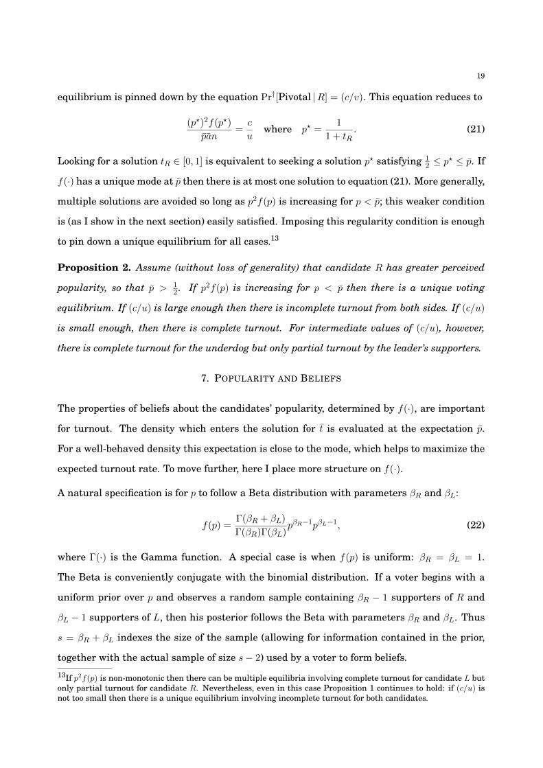
to pin down a unique equilibrium for all cases.13

Proposition 2. Assume (without loss of generality) that candidate R has greater perceived

popularity, so that p >

12 . If p

2f(p) is increasing for p < p then there is a unique voting

equilibrium. If (c/u) is large enough then there is incomplete turnout from both sides. If (c/u)

is small enough, then there is complete turnout. For intermediate values of (c/u), however,

there is complete turnout for the underdog but only partial turnout by the leader’s supporters.

7. POPULARITY AND BELIEFS

The properties of beliefs about the candidates’ popularity, determined by f(·), are important

for turnout. The density which enters the solution for ¯

t is evaluated at the expectation p.

For a well-behaved density this expectation is close to the mode, which helps to maximize the

expected turnout rate. To move further, here I place more structure on f(·).

A natural specification is for p to follow a Beta distribution with parameters �

R

and �

L

:

f(p) =

�(�

R

+ �

L

)

�(�

R

)�(�

L

)

p

�R�1p

�L�1, (22)

where �(·) is the Gamma function. A special case is when f(p) is uniform: �

R

= �

L

= 1.

The Beta is conveniently conjugate with the binomial distribution. If a voter begins with a

uniform prior over p and observes a random sample containing �

R

� 1 supporters of R and

�

L

� 1 supporters of L, then his posterior follows the Beta with parameters �

R

and �

L

. Thus

s = �

R

+ �

L

indexes the size of the sample (allowing for information contained in the prior,

together with the actual sample of size s� 2) used by a voter to form beliefs.13If p2f(p) is non-monotonic then there can be multiple equilibria involving complete turnout for candidate L butonly partial turnout for candidate R. Nevertheless, even in this case Proposition 1 continues to hold: if (c/u) isnot too small then there is a unique equilibrium involving incomplete turnout for both candidates.

20

The mean of the Beta is p = �

R

/(�

R

+ �

L

). The density may be written in terms of p and a

parameter s which corresponds to the information available to a voter; as explained above,

s � 2 would corresponds to the sample size of an opinion poll, yielding an effective precision

proportional to s once the prior is taken into account. Using this formulation,

f(p) =

�(s)

�(ps)�((1� p)s)

p

ps�1(1� p)

(1�p)s�1. (23)

It is straightforward to confirm that p2f(p) is increasing for p < p, and so the Beta specification

meets the condition of Proposition 2; there is a unique voting equilibrium. The density f(p)

can be substituted into the turnout solution from Proposition 1. Doing so:

¯

t =

�(s)

�(ps)�((1� p)s)

2u[p

p

(1� p)

(1�p)]

s

cn

. (24)

To see things a little more clearly, and when s is large enough, the Beta density can be ap-

proximated with a normal distribution. The variance of the Beta, in terms of s and the mean

p, satisfies var[p] = p(1� p)/(s+ 1). So, using a normal approximation,

f(p) ⇡

ss+ 1

2⇡p(1� p)

exp

✓�

(s+ 1)(p� p)

2

2p(1� p)

◆, (25)

where here ⇡ indicates the mathematical constant and not a model parameter. When evalu-

ated at p the exponential term disappears, so generating the next result.

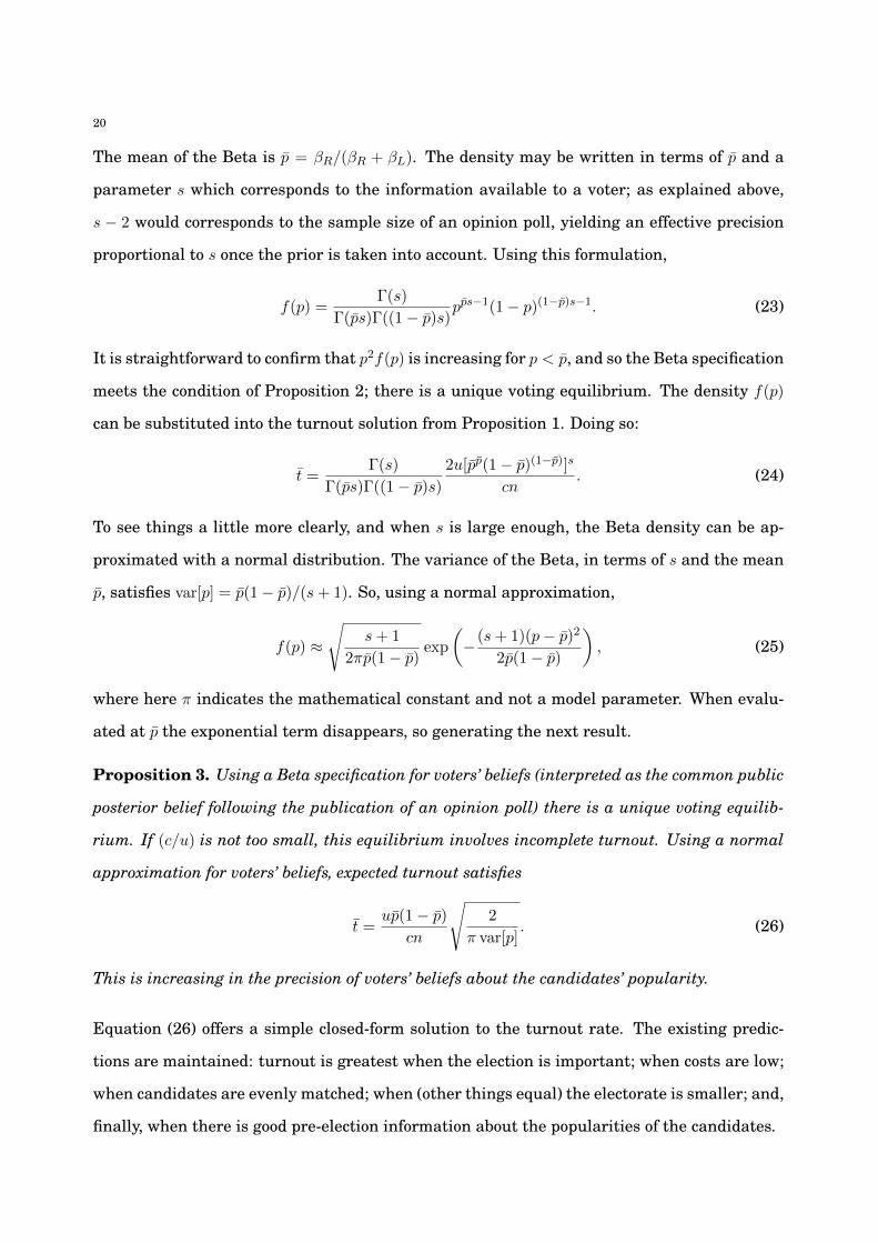
Proposition 3. Using a Beta specification for voters’ beliefs (interpreted as the common public

posterior belief following the publication of an opinion poll) there is a unique voting equilib-

rium. If (c/u) is not too small, this equilibrium involves incomplete turnout. Using a normal

approximation for voters’ beliefs, expected turnout satisfies

¯

t =

up(1� p)

cn

s2

⇡ var[p]

. (26)

This is increasing in the precision of voters’ beliefs about the candidates’ popularity.

Equation (26) offers a simple closed-form solution to the turnout rate. The existing predic-

tions are maintained: turnout is greatest when the election is important; when costs are low;

when candidates are evenly matched; when (other things equal) the electorate is smaller; and,

finally, when there is good pre-election information about the popularities of the candidates.

21

The final prediction of Proposition 3 is supported by recent empirical work. Gentzkow (2006)

used between-market variation in the timing of the introduction of television to identify an

negative effect on turnout. The introduction of television “caused sharp drops in consumption

of newspapers and radio” and “reduced citizens’ knowledge of politics as measured in election

surveys” (Gentzkow, 2006, p. 932). This switch away from other media, which in turn reduced

the extent of electoral coverage, particularly in off-year congressional elections, is consistent

with an increase in var[p] and so a fall in turnout rates.

8. ASYMMETRIC AND IDIOSYNCRATIC VOTING COSTS

In the core model the payoff parameters u and c are the same for everyone. Here I extend the

model by varying the cost of voting; keeping u fixed involves little loss of generality because

the ratio (c/u) determines a voter’s participation decision.

I begin by supposing that payoff parameters are common within each faction of the electorate,

but differ between the two factions. Using an obvious notation, a voting equilibrium with

incomplete turnout on both sides is pinned down by the two equalities

Pr

†[Pivotal |L] =

c

L

u

and Pr

†[Pivotal |R] =

c

R

u

. (27)

Lemma 3 (concerning the nature of pivotal probabilities in larger electorates) continues to

hold here. However, Lemma 4 does not; it is no longer the case that the critical threshold

p

?

= t

L

/(t

L

+ t

R

) for R’s popularity must equal the prior expectation p. Instead, combining the

two equilibrium conditions from equation (27) yields

p

?

=

pc

R

pc

R

+ (1� p)c

L

. (28)

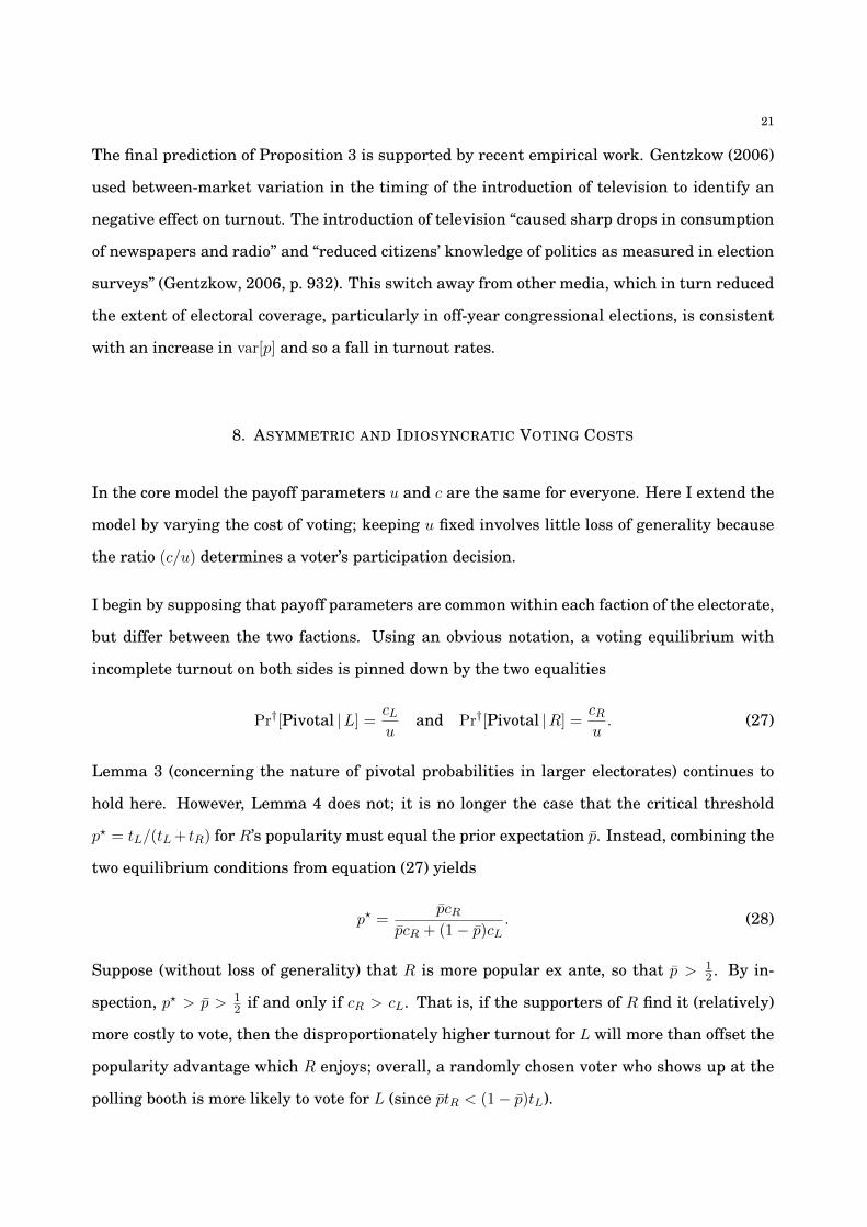
Suppose (without loss of generality) that R is more popular ex ante, so that p >

12 . By in-

spection, p? > p >

12 if and only if c

R

> c

L

. That is, if the supporters of R find it (relatively)

more costly to vote, then the disproportionately higher turnout for L will more than offset the

popularity advantage which R enjoys; overall, a randomly chosen voter who shows up at the

polling booth is more likely to vote for L (since pt

R

< (1� p)t

L

).

22

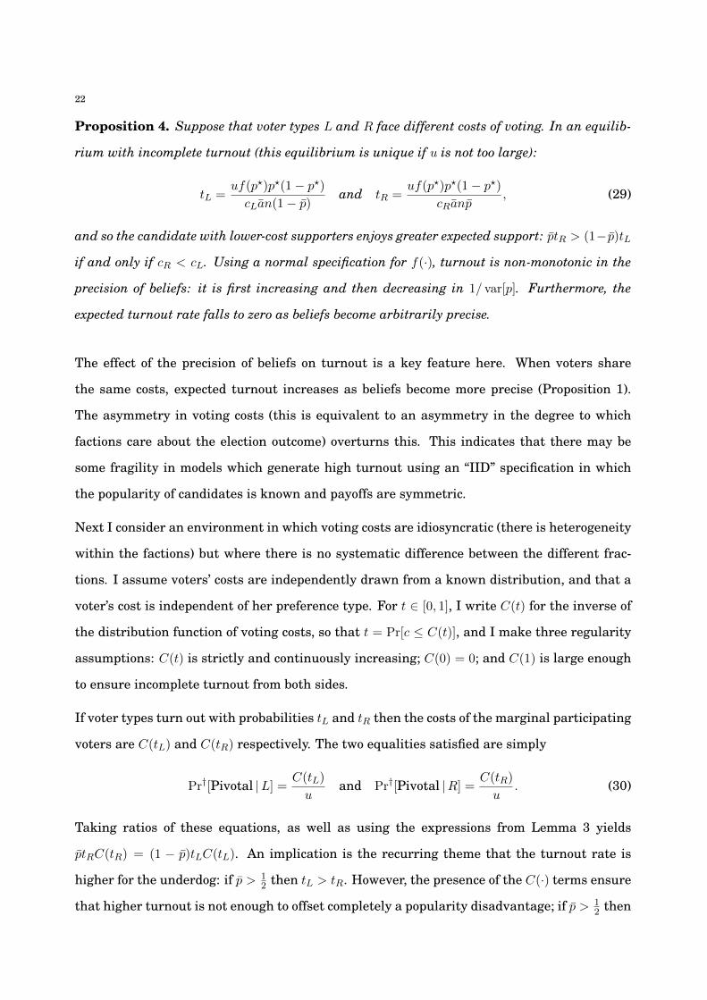
Proposition 4. Suppose that voter types L and R face different costs of voting. In an equilib-

rium with incomplete turnout (this equilibrium is unique if u is not too large):

t

L

=

uf(p

?

)p

?

(1� p

?

)

c

L

an(1� p)

and t

R

=

uf(p

?

)p

?

(1� p

?

)

c

R

anp

, (29)

and so the candidate with lower-cost supporters enjoys greater expected support: ptR

> (1� p)t

L

if and only if cR

< c

L

. Using a normal specification for f(·), turnout is non-monotonic in the

precision of beliefs: it is first increasing and then decreasing in 1/ var[p]. Furthermore, the

expected turnout rate falls to zero as beliefs become arbitrarily precise.

The effect of the precision of beliefs on turnout is a key feature here. When voters share

the same costs, expected turnout increases as beliefs become more precise (Proposition 1).

The asymmetry in voting costs (this is equivalent to an asymmetry in the degree to which

factions care about the election outcome) overturns this. This indicates that there may be

some fragility in models which generate high turnout using an “IID” specification in which

the popularity of candidates is known and payoffs are symmetric.

Next I consider an environment in which voting costs are idiosyncratic (there is heterogeneity

within the factions) but where there is no systematic difference between the different frac-

tions. I assume voters’ costs are independently drawn from a known distribution, and that a

voter’s cost is independent of her preference type. For t 2 [0, 1], I write C(t) for the inverse of

the distribution function of voting costs, so that t = Pr[c C(t)], and I make three regularity

assumptions: C(t) is strictly and continuously increasing; C(0) = 0; and C(1) is large enough

to ensure incomplete turnout from both sides.

If voter types turn out with probabilities t

L

and t

R

then the costs of the marginal participating

voters are C(t

L

) and C(t

R

) respectively. The two equalities satisfied are simply

Pr

†[Pivotal |L] =

C(t

L

)

u

and Pr

†[Pivotal |R] =

C(t

R

)

u

. (30)

Taking ratios of these equations, as well as using the expressions from Lemma 3 yields

pt

R

C(t

R

) = (1 � p)t

L

C(t

L

). An implication is the recurring theme that the turnout rate is

higher for the underdog: if p >

12 then t

L

> t

R

. However, the presence of the C(·) terms ensure

that higher turnout is not enough to offset completely a popularity disadvantage; if p >

12 then

23

the critical popularity threshold p

? satisfies 12 < p

?

< p. Once again, if R is less popular than

she is expected to be (so that p < p) then she may still win (if p > p

?) but also she may lose

despite being the more popular candidate; this happens when 12 < p < p

?.

The equilibrium is very easy to characterize when costs are uniformly distributed. If c ⇠

U [0, 1] then tC(t) = t

2, and the equality pt

R

C(t

R

) = (1� p)t

L

C(t

L

) yields

p

?

1� p

?

=

rp

1� p

. (31)

Hence, under the uniform specification the relative turnout of the two factions is uniquely

determined by the expected popularity of one candidate relative to the other; the other pa-

rameters of the model have no major role to play. All of these observations, together with the

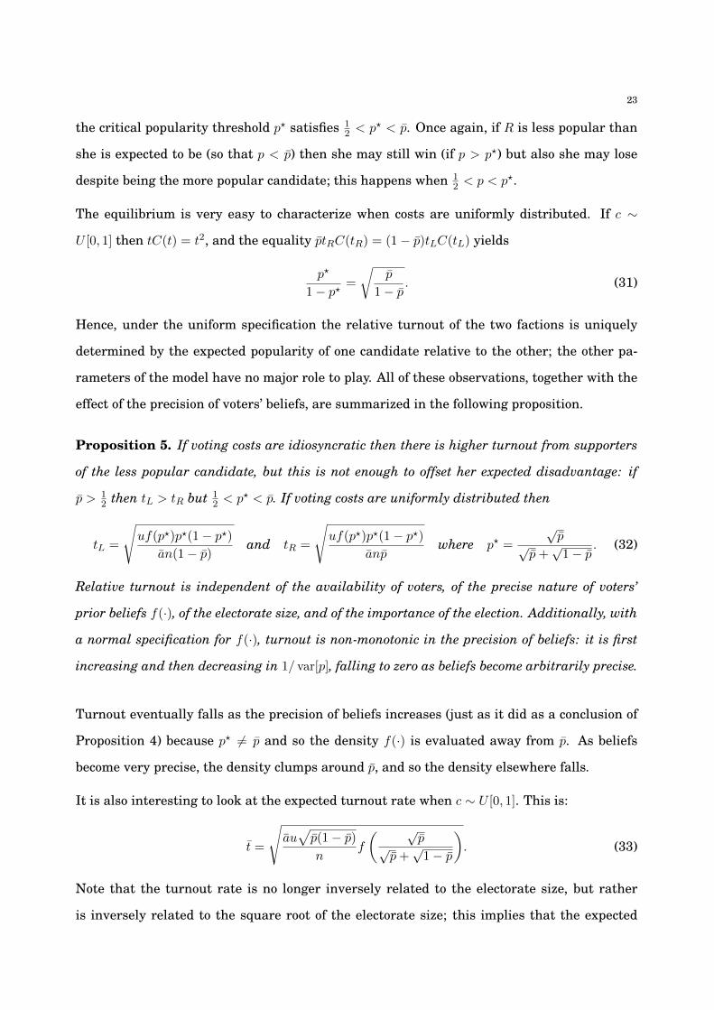
effect of the precision of voters’ beliefs, are summarized in the following proposition.

Proposition 5. If voting costs are idiosyncratic then there is higher turnout from supporters

of the less popular candidate, but this is not enough to offset her expected disadvantage: if

p >

12 then t

L

> t

R

but 12 < p

?

< p. If voting costs are uniformly distributed then

t

L

=

suf(p

?

)p

?

(1� p

?

)

an(1� p)

and t

R

=

suf(p

?

)p

?

(1� p

?

)

anp

where p

?

=

p

p

p

p+

p

1� p

. (32)

Relative turnout is independent of the availability of voters, of the precise nature of voters’

prior beliefs f(·), of the electorate size, and of the importance of the election. Additionally, with

a normal specification for f(·), turnout is non-monotonic in the precision of beliefs: it is first

increasing and then decreasing in 1/ var[p], falling to zero as beliefs become arbitrarily precise.

Turnout eventually falls as the precision of beliefs increases (just as it did as a conclusion of

Proposition 4) because p

?

6= p and so the density f(·) is evaluated away from p. As beliefs

become very precise, the density clumps around p, and so the density elsewhere falls.

It is also interesting to look at the expected turnout rate when c ⇠ U [0, 1]. This is:

¯

t =

sau

pp(1� p)

n

f

✓p

p

p

p+

p

1� p

◆. (33)

Note that the turnout rate is no longer inversely related to the electorate size, but rather

is inversely related to the square root of the electorate size; this implies that the expected

24

total turnout ¯

tn is increasing with n. This contrasts with the homogenous-costs case, where

total expected turnout is independent of n. Note also that the turnout rate is increasing in

the expected availability of voters. These features are because voting costs are heterogeneous

with a support that extends down to zero. (Recall that I am using a uniform distribution here,

so that c ⇠ U [0, 1].) Those who turn out are those with the lowest costs, and there are simply

more of them as the electorate size and voters’ availability both grow.

A key message from the results of this section is that endogenous turnout causes the familiar

effect of enhancing the chances of the underdog; indeed, it generates situations in which the

a truly popular candidate loses. However, only when payoffs are common to all electors is

this effect so strong as to offset exactly any prior asymmetry in popularity. With intra-faction

variation in costs, there is only a partial pro-underdog bias in turnout.

9. TURNOUT IN LARGER ELECTORATES

In this section I tackle two issues: the properties of turnout as the electorate size grows, and

the use of approximations to the pivotal probabilities in my solution concept.

For equilibria with incomplete turnout, the expected turnout rate satisfies (Proposition 1)

¯

t =

2p(1� p)f(p)u

cn

. (34)

Other things equal, this falls with the electorate size, and so it is tempting to conclude that

the turnout rate will be low in large electorates; this is at the heart of the turnout paradox.

This conclusion should not be reached too hastily. In larger electorates the issues at stake are

different, the pattern of preferences may differ, and voters may have different information

available to them. Focusing on the first point, in a larger electorate the stakes are likely to be

higher.14 At a basic level, this is simply because of the number of people who are affected by

14As noted in my introductory remarks, this point has been made elsewhere, most notably by Edlin, Gelman, andKaplan (2007), but also in other work, such as articles by Fowler and Kam (2007), Loewen (2010), and Dawes,Loewen, and Fowler (2011). Past empirical work has reported evidence that voters incorporate so-called sociotropic(society level) factors (Kinder and Kiewiet, 1981; MacKuen, Erikson, and Stimson, 1992; Clarke and Stewart,1994; Mutz and Mondak, 1997); participation in elections is associated with measures of social cooperation, suchas jury service and census response (Knack, 1992b,a; Knack and Kropf, 1998); and experimental researchers havereported an association between the self-reported electoral turnout behavior of subjects and the extent of altruisticallocations in a dictator game (Fowler, 2006). Notice that the social preferences considered here are derived froma voter’s anticipated instrumental effect on the electoral outcome, and so differ from the addition of a civic dutyterm to a voter’s payoff (Riker and Ordeshook, 1968; Goldfarb and Sigelman, 2010), from the use of an ethical

25

the outcome. If a voter has any element of other-regarding social preferences (he cares about

others, whether altruistically or paternalistically) then the weight of the election outcome will

increase with n.

Adopting this argument formally, suppose that the instrumental payoff from influencing the

winner is contingent on the electorate size, and so I denote it as u

n

. Suppose that this payoff

is linearly increasing in n, so that

u

n

= u+ bn. (35)

The payoff u is the private implication of the outcome, whereas b is the per-person impact on

others from the perspective of an individual voter. The parameter b reflects the voter’s social

preferences. (Many critiques of instrumental theories implicitly assume that b = 0, without

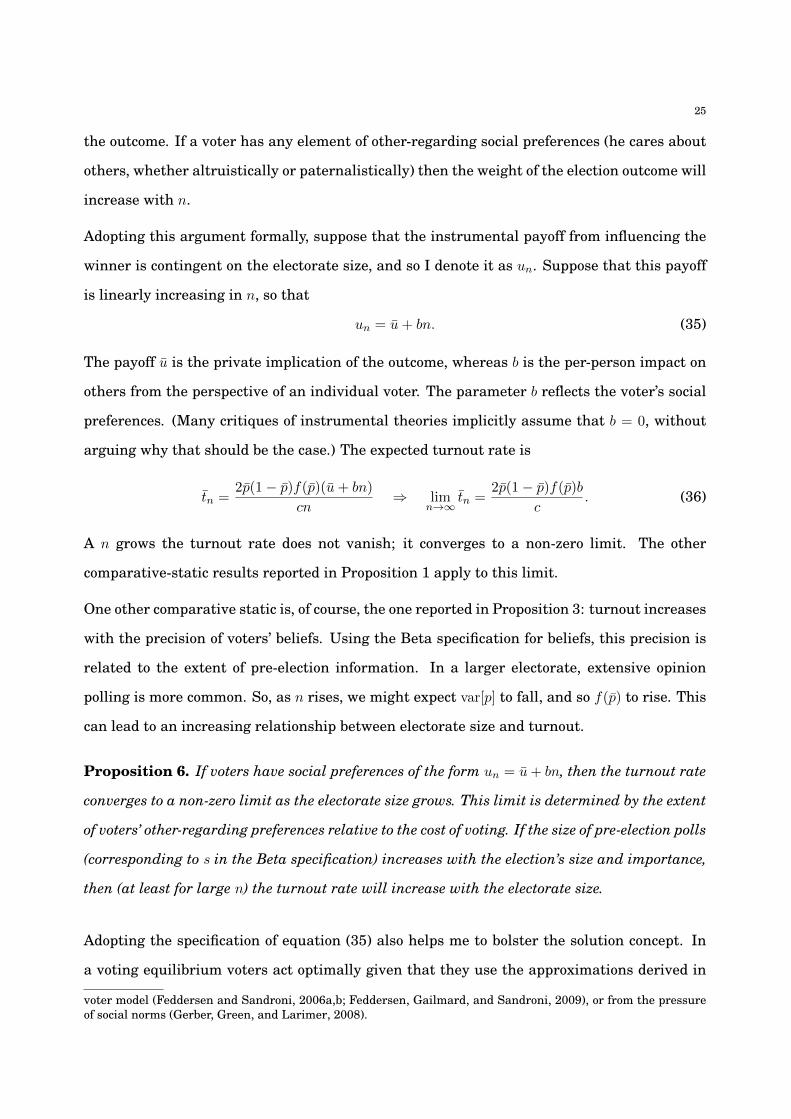
arguing why that should be the case.) The expected turnout rate is

¯

t

n

=

2p(1� p)f(p)(u+ bn)

cn

) lim

n!1¯

t

n

=

2p(1� p)f(p)b

c

. (36)

A n grows the turnout rate does not vanish; it converges to a non-zero limit. The other

comparative-static results reported in Proposition 1 apply to this limit.

One other comparative static is, of course, the one reported in Proposition 3: turnout increases

with the precision of voters’ beliefs. Using the Beta specification for beliefs, this precision is

related to the extent of pre-election information. In a larger electorate, extensive opinion

polling is more common. So, as n rises, we might expect var[p] to fall, and so f(p) to rise. This

can lead to an increasing relationship between electorate size and turnout.

Proposition 6. If voters have social preferences of the form u

n

= u+ bn, then the turnout rate

converges to a non-zero limit as the electorate size grows. This limit is determined by the extent

of voters’ other-regarding preferences relative to the cost of voting. If the size of pre-election polls

(corresponding to s in the Beta specification) increases with the election’s size and importance,

then (at least for large n) the turnout rate will increase with the electorate size.

Adopting the specification of equation (35) also helps me to bolster the solution concept. In

a voting equilibrium voters act optimally given that they use the approximations derived in

voter model (Feddersen and Sandroni, 2006a,b; Feddersen, Gailmard, and Sandroni, 2009), or from the pressureof social norms (Gerber, Green, and Larimer, 2008).

26

Lemma 3. These approximations improve as n grows; but of course, as n grows the size of the

pivotal probabilities shrinks, and so (when payoffs do not depend on n) the turnout rate does

so too. Thus, to use limiting values properly, I need to ensure that the equilibrium turnout

rates do not vanish. Allowing payoffs to increase linearly with n is a way to do this. (Arguably,

it is no more restrictive than assuming that u is independent of n.) Doing so, a single pair of

turnout probabilities can act as an appropriate solution for all larger electorates.

To see this idea in action, here I adopt a variant of the equilibrium concept used by Myatt

(2007) and Dewan and Myatt (2007). This concept is defined relative to a sequence of voting

games. Separate equilibrium turnout probabilities are not specified for each electorate size.

Instead, I take a pair of turnout probabilities and ask whether a voter can do more than "

better in large electorates; thus I look for a kind of "-equilibrium. I then seek the turnout

probabilities for which " can be made arbitrarily small in large electorates.

Definition. A pair of turnout probabilities t

L

and t

R

is an asymptotic voting equilibrium if a

voter’s expected payoff gain from switching his turnout decision converges to zero as n ! 1.

If the instrumental payoff increases linearly with n (or more generally if limn!1(u

n

/n) = b)

then the asymptotic voting equilibrium solution concept makes a unique prediction.

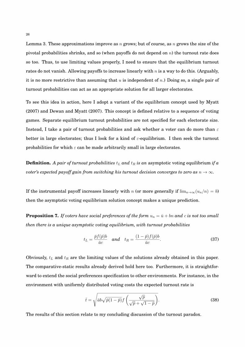
Proposition 7. If voters have social preferences of the form u

n

= u+ bn and c is not too small

then there is a unique asymptotic voting equilibrium, with turnout probabilities

t

L

=

pf(p)b

ac

and t

R

=

(1� p)f(p)b

ac

. (37)

Obviously, tL

and t

R

are the limiting values of the solutions already obtained in this paper.

The comparative-static results already derived hold here too. Furthermore, it is straightfor-

ward to extend the social preferences specification to other environments. For instance, in the

environment with uniformly distributed voting costs the expected turnout rate is

¯

t =

s

ab

pp(1� p)f

✓p

p

p

p+

p

1� p

◆. (38)

The results of this section relate to my concluding discussion of the turnout paradox.

27

10. RESOLVING THE TURNOUT PARADOX

It is often claimed that rational-choice theory predicts extremely low turnout. The classic

reasoning is that if the turnout rate were high then the probability of a tie in a large electorate

is far too low to justify the cost of voting. Indeed, in a critical assessment of rational-choice

methods, Green and Shapiro (1994, Chapter 4) claimed:

“Although rational citizens may care a great deal about which person or group

wins the election, an analysis of the instrumental value of voting suggests that

they will nevertheless balk at the prospect of contributing to a collective cause

since it is readily apparent that any one vote has an infinitesimal probability of

altering the election outcome.”

It is true that, other things equal, the probability of a tie declines as the electorate size grows.

This, however, does not justify the “too low to vote” conclusion. It is not clear that the probabil-

ity is “infinitesimal” and it is not “readily apparent” that there is no hope for an instrumental

explanation for the turnout decision. What is needed is an assessment of precisely how big

or small the pivotal probability is. To move forward I proceed with a calibration exercise: I

choose reasonable parameters and ask whether plausible levels of turnout emerge.

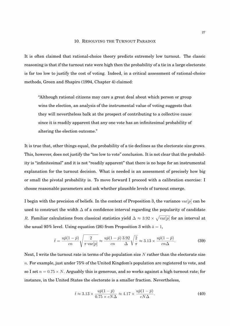
I begin with the precision of beliefs. In the context of Proposition 3, the variance var[p] can be

used to construct the width � of a confidence interval regarding the popularity of candidate

R. Familiar calculations from classical statistics yield � ⇡ 3.92 ⇥

pvar[p] for an interval at

the usual 95% level. Using equation (26) from Proposition 3 with a = 1,

¯

t =

up(1� p)

cn

s2

⇡ var[p]

⇡

up(1� p)

cn

3.92

�

r2

⇡

⇡ 3.13⇥

up(1� p)

cn�

. (39)

Next, I write the turnout rate in terms of the population size N rather than the electorate size

n. For example, just under 75% of the United Kingdom’s population are registered to vote, and

so I set n = 0.75⇥N . Arguably this is generous, and so works against a high turnout rate; for

instance, in the United States the electorate is a smaller fraction. Nevertheless,

¯

t ⇡ 3.13⇥

up(1� p)

0.75⇥ cN�

⇡ 4.17⇥

up(1� p)

cN�

. (40)

28

Finally, I pick a value for the expected popularity of the leading candidate. Obviously, if the

candidates are seen as evenly matched then turnout is higher. So, to work against higher

turnout I choose a more unbalanced 60 : 40 split, so that p = 0.6. Doing so,

¯

t ⇡ 4.17⇥

u⇥ 0.6⇥ 0.4

cN�

= 4.17⇥ 0.24⇥

u

cN�

⇡

(u/c)

N�

. (41)

I record this calibration exercise as a simple proposition.

Proposition 8. Consider a region in which 75% of the population are eligible to vote, where a

95% confidence interval for popularity of the leading candidate is centered at 60%. Then,

Expected Turnout Rate ⇡

Instrumental Benefit/Voting CostPopulation ⇥ Width of 95% Confidence Interval

. (42)

Hence, in a region of 100,000 people, such as the city of Cambridge (either Massachusetts or

England), if a confidence interval for the more popular candidate ranges from 57% to 62% (the

interval following a typical opinion poll), and if voters are willing to participate for a 1-in-2,500

chance of influencing the outcome, then turnout should exceed 50%.

This is the vignette from the introductory remarks to this paper. To explain substantial

turnout (50%) under reasonable conditions I need voters who are willing to show up for a

1-in-2,500 of influencing the lives of 100,000 fellow citizens.

The required probability of 1-in-2,500 is small, but many might find it a stretch to call this

an “infinitesimal probability of altering the election outcome” as Green and Shapiro (1994)

claimed. Of course, the required cost-to-benefit ratio (for in this case (c/u) = 0.0004) falls as

the population size expands and as I deviate from the baseline model.

Taking the “larger electorate” point first, for a population of 10,000,000 I need voters who are

willing to show up for the rather longer odds of 1-in-250,000. If voting costs $5, then this

places an implicit value (roughly speaking) of $1,250,000 for changing the outcome. For the

private consequences of an election result (a change in tax rates, public good provision, and so

on) this seems large, and so the odds of influencing the outcome seem small. However, a tiny

element of social preferences is enough to generate participation for such odds. Revisiting

a scenario described in my introductory remarks, suppose that a paternalistic voter believes

that the right election outcome will help the typical population member by $250 per year

29

over a five year term; a modest impact of $1,250. If this voter’s concern for others is only

0.0001 (that is, one hundredth of one per cent) then the implicit value of the election to him

is indeed $1,250,000, and this voter would participate for the stated chance of influencing the

outcome. Social preferences scale, of course, and so the same extent (0.01%) of other-regarding

preferences would work with a population of 1,000,000 (the example from the introduction of

this paper) as well as a population of 100,000,000 (a national election in a large country).

Of course, a narrowly self-interested and instrumentally motivated citizen might not turn

out for the odds discussed here. From this, the Green and Shapiro (1994) argument invites

researchers to abandon the use of rational-choice methods; their critique asks for the assump-

tion that voters are dumb in order to cling on to the assumption of very narrow selfishness.

However, allowing smart voters to be very mildly (as little as 0.01%) socially motivated can

explain significant turnout; rational choice does not require narrow selfishness.

Moving to deviations from the basic model, turnout is lower when (for instance) costs are

heterogeneous. Nevertheless, limited social preferences are again sufficient to generate rea-

sonable turnout. Moreover, the step away from the stark nature of the core model also moves

the “underdog effect” away from the complete unravelling of the leading candidate’s support

advantage, to yield a more nuanced conclusion: those who are seen as more popular may

sometimes lose to a less popular rival, but that loss is far from inevitable.

CONCLUDING REMARKS

Aldrich (1993, p. 246) observed that “turning out to vote is the most common act citizens take

in a democracy” and yet “it is not well understood.” To provide this understanding, the theory

presented here uses a simple model with largely standard features, but develops fully the

(sadly neglected) insights of Good and Mayer (1975) regarding the crucial nature of aggregate

uncertainty. The conclusions are that significant turnout is consistent with goal-oriented

voters under reasonable parameter considerations; the underdog effect offsets (although not

necessarily completely) the advantage of a perceived leading candidate via greater turnout

for her competitor; and the precision of voters’ beliefs, as well as other more familiar factors,

has a predictable impact on turnout in elections. The model offers a framework which may

help to develop further other studies of democratic systems.

30

APPENDIX A. OMITTED PROOFS

Proof of Lemma 1. For each � 2 � and n define P

n

(�) ⌘

R� [

Qm

i=0v�ii

]

n

h(v) dv, so that

Pr[b |h(·)] =

�(n+ 1)Qn

i=0 �(bi + 1)

P

n

�b

n

�.

P

n

(�) is a continuous function of � over the compact set �. The first step of the proof is toshow that P

n

(�) can be replaced with h(�)

R� [

Qm

i=0v�ii

]

n

dv as n grows large. To take this step,begin by noting that the quasi-concave function

Qm

i=0v�ii

is maximized by v = �. For small" > 0 define �

"

= {v 2 � |

Qm

i=0v�ii

�

Qm

i=0��ii

� "}. This is a compact and convex neighborhoodof �. A lower bound to an expression of interest can be obtained:

P

n

(�)R� [

Qm

i=0v�ii

]

n

dv

�

R�"

[

Qm

i=0v�ii

]

n

h(v) dv

R� [

Qm

i=0v�ii

]

n

dv

�

min

v2�"{h(v)}

1 +R

n

where R

n

=

R�/�"

[

Qm

i=0v�ii

]

n

dv

R�"

[

Qm

i=0v�ii

]

n

dv

.

and where �/�

"

⌘ {v 2 � |

Qm

i=0v�ii

<

Qm

i=0��ii

� "}. Similarly,

P

n

(�)R� [

Qm

i=0v�ii

]

n

dv

R�/�"

[

Qm

i=0v�ii

]

n

h(v) dv +

R�"

[

Qm

i=0v�ii

]

n

h(v) dv

R� [

Qm

i=0v�ii

]

n

dv

max

v2�{h(v)}Rn

+max

v2�"{h(v)}

1 +R

n

,

where R

n

is defined as before, and so

max

v2�{h(v)}Rn

+max

v2�"{h(v)}

1 +R

n

�

P

n

(�)R� [

Qm

i=0v�ii

]

n

dv

�

min

v2�"{h(v)}

1 +R

n

.

The maxima are well-defined: h(v) is continuous and � and �

"

are compact. Examining R

n

,

R

n

R�/�"

[

Qm

i=0v�ii

]

n

dv

R�"

[

Qm

i=0��ii

� "]

n

dv

=

1R�"

dv

Z

�/�"

Qm

i=0v�iiQ

m

i=0��ii

� "

�n

dv �! 0 as n ! 1,

where the final claim follows becauseQ

m

i=0v�ii

<

Qm

i=0��ii

� " for all v 2 �/�

"

. Hence:

max

v2�"

{h(v)} � lim

n!1

P

n

(�)R� [

Qm

i=0v�ii

]

n

dv

�� min

v2�"

{h(v)}.

By choosing " small enough I can ensure that both min

v2�"{h(v)} and max

v2�"{h(v)} arearbitrarily close to h(�), since h(·) is continuous, and so I conclude that

lim

n!1

P

n

(�)R� [

Qm

i=0v�ii

]

n

dv

�= h(�).

Notice also that each member of the sequence of functions (indexed by n) is continuous in �,and so is the limiting function h(�). Thus, looking across the compact set �, the convergence

31

reported above is uniform. That is,

lim

n!1sup

�2�

����P

n

(�)R� [

Qm

i=0v�ii

]

n

dv

� h(�)

���� = 0.

With the first step of the proof in hand in hand, I turn to the probability of b 2 �

†n

.

n

m

Pr[b |h(·)] = n

m

�(n+ 1)Qm

i=0 �(bi + 1)

P

n

�b

n

�

= n

m

�(n+ 1)

�(n+m+ 1)

P

n

�b

n

�

R�

hQm

i=0v(bi/n)i

in

dv

⇥

Z

�

�(n+m+ 1)Qm

i=0 �(bi + 1)

hYm

i=0v

(bi/n)i

in

| {z }density of Dirichlet

dv

=

n

m

(n+ 1)⇥ (n+ 2)⇥ · · ·⇥ (n+m)

⇥

P

n

�b

n

�

R�

hQm

i=0v(bi/n)i

in

dv

.

The final equality holds because the third term in the previous expression is the integral ofa Dirichlet density. Looking at the final line, the first ratio converges to one as n ! 1. Thesecond ratio is the term considered earlier, evaluated at � = b/n. The convergence establishedpreviously was uniform. I conclude that lim

n!1max

b2�†n|n

m

Pr[b |h(·)]� h(�)| = 0. ⇤

Proof of Lemma 2. From (6) in the text, nPr[b

L

= b

R

] =

1n

Pbn/2cz=0 n

2Pr[b

L

= b

R

= z | i]. UsingLemma 1, nPr[b

L

= b

R

= z] converges uniformly. That is,

lim

n!1max

z2{0,1,...,bn/2c}

����n2Pr[b

L

= b

R

= z]� h

✓n� 2z

n

,

z

n

,

z

n

| i

◆���� = 0

) lim

n!1nPr[b

L

= b

R

| i] = lim

n!1

1

n

Xbn/2c

z=0h

✓n� 2z

n

,

z

n

,

z

n

| i

◆,

where this equality holds so long as the right-hand side limit is well-defined. As noted in thetext, the right-hand side defines a Riemann integral of h(1 � 2x, x, x) over the range [0, 1/2],and so converges to

R 1/20 h(1�2x, x, x) dx as n ! 1. Similar calculations apply to near ties. ⇤

Proof of Lemma 3. Substitute the conditional densities from (13) into (12). ⇤

Proof of Lemma 4. As noted in the main text, an inspection of (17) shows thatPr

†[Pivotal |L] = Pr

†[Pivotal |R] if and only if p = p

?

= t

L

/(t

L

+ t

R

). ⇤

Proof of Lemma 5. I have assumed that c <

v

2 and so there must be positive turnout from atleast one voter type. This implies that max{t

L

, t

R

} > 0, and so p

? (from Lemma 3) is defined.If t

R

� t

L

then there is positive turnout from the supporters of R and so Pr

†[Pivotal |R] > 0.

t

R

� t

L

implies that p

?

12 and so, given that p >

12 , the expressions in (17) ensure that

Pr

†[Pivotal |R] < Pr

†[Pivotal |L]. This means there is a strict incentive for supporters of L to

participate, and so t

L

= 1. Hence, tR

� t

L

can only hold if tL

= t

R

= 1; so, it cannot be the casethat t

R

> t

L

. The final claim of the lemma follows directly. ⇤

32

Proof of Proposition 1. Using equation (18) and equating to (c/u) readily yields ¯

t. Combiningthis with the fact that t

L

/(t

L

+ t

R

) = p from Lemma 4 yields the expressions for t

L

and t

R

inequation (19). The comparative-static claims follow by inspection. The proposition says that“if (c/u) is not too small.” This is so that the solutions satisfy max{t

L

, t

R

} < 1; the relevantinequality is stated in the main text as equation (20). The uniqueness of this incomplete-turnout equilibrium for (c/u) satisfying this inequality is established by Proposition 2. ⇤

Proof of Proposition 2. From Lemma 5, the possible equilibria are: (i) complete turnout fromboth factions, so that t

L

= t

R

= 1; (ii) complete turnout for the underdog, so that tR

< t

L

= 1;and (iii) incomplete turnout from both factions, so that t

L

< t

R

< 1.

Case (i). If t

L

= t

R

= 1 then p

?

=

12 . Given that p �

12 , this means that Pr

†[Pivotal |L] �

Pr

†[Pivotal |R]. Hence, a necessary and sufficient condition for this to be an equilibrium is

Pr

†[Pivotal |R] �

c

v

, f(p

?

)(p

?

)

2�

canp

v

where p

?

=

1

2

. (i)

Case (ii). If tR

< t

L

= 1 then p

?

= 1/(1 + t

R

) >

12 . For this to be an equilibrium the supporters

of candidate R must be indifferent and so Pr

†[Pivotal |R] = (c/v). The supporters of L must

also be willing to turn out, which is so if and only if Pr†[Pivotal |L] � Pr

†[Pivotal |R] , p

?

p.There is an equilibrium of this kind if and only if there is a p

? satisfying

f(p

?

)(p

?

)

2=

canp

v

where1

2

< p

?

p. (ii)

Case (iii). If t

R

< t

L

< 1 then p

?

= p. The turnout rates for such an equilibrium are re-ported in Proposition 1. As noted in the text, there is an equilibrium of this kind only wheninequality (20) is satisfied, which holds if and only if

f(p

?

)(p

?

)

2<

canp

v

where p

?

= p. (iii)

Notice that f(p)p

2 is a continuous in p and achieves a maximum on the compact interval[(1/2), p]. If vmax

p2[(1/2),p][f(p)p2] < canp neither (i) nor (ii) are satisfied but (iii) is, and so

there is a unique equilibrium with incomplete turnout from both factions. This proves theuniqueness claim of Proposition 1; note that this does not require monotonicity of f(p)p2.

Now, however, suppose that f(p)p2 is strictly increasing over the relevant interval (as is stip-ulated in the proposition) and so is maximized at p = p and minimized at p =

12 . Thus,

if v[f(p)p

2] < canp then (iii) holds but (i) and (ii) do not. However, if v[f(p)p

2] � canp

then (iii) fails. If v[f(1/2)(1/2)

2] � canp then (i) holds, but (ii) must fail, and so there is

a unique equilibrium with complete turnout from everyone. The remaining case is whenv[f(p)p

2] � canp > v[f(1/2)(1/2)

2]. Neither (i) nor (Iii) hold. However, f(p)p2 is continuous

and strictly monotonic, and so (ii) has a unique solution in the relevant interval; hence thereis a unique equilibrium involving complete turnout for the underdog. ⇤

33

Proof of Proposition 3. The expression for ¯

t is obtained by substituting in the normal densityfor f(p). The comparative-static claim holds by inspection. ⇤

Proof of Proposition 4. Substituting in the expressions for Pr

†[Pivotal |L] and Pr

†[Pivotal |R],

the equilibrium conditions from equation (27) become

f(p

?

)(1� p

?

)

an(t

L

+ t

R

)(1� p)

=

c

L

u

andf(p

?

)p

?

an(t

L

+ t

R

)p

=

c

R

u

.

Taking ratios of these two equations,

p

?

(1� p)

p(1� p

?

)

=

c

R

c

L

,

which is re-arranged to yield equation (28). Notice that p

?

= p , c

L

= c

R

. Solving for theequilibrium turnouts is straightforward; simple algebra confirms the solutions stated in theproposition, and pt

R

> (1� p)t

L

, c

R

< c

L

by inspection. The turnout rates depend on f(p

?

).Away from the mean (for p

?

6= p) the density of the normal is non-monotonic (first increasing,and then decreasing) as the variance falls (the precision rises). ⇤

Proof of Proposition 5. The first claim follows from an inspection of equation (31). Re-arranging this equation yields the solution for p

? displayed in equation (32). The solutionsfor t

L

and t

R

are straightforwardly obtained by solving the equilibrium conditions after set-ting C(t

L

) = t

L

and C(t

R

) = t

R

. The remaining claims follow by inspection. ⇤

Proof of Proposition 6. The claims follow from an inspection of equation (36). ⇤

Proof of Proposition 7. Fixing turnout probabilities t

L

and t

R

, a voter’s gain or loss fromswitching his participation decision converges to zero as n ! 1 if and only if the expectedbenefit from voting converges to c. So, for this pair of turnout probabilities to yield an asymp-totic voting equilibrium,

lim

n!1(u+ bn) Pr[Pivotal |L] = lim

n!1(u+ bn) Pr[Pivotal |R] = c.

Now, using Lemma 3,

(u+ bn) Pr[Pivotal |L] = nPr[Pivotal |L]⇥u+ bn

n

!

bf(p

?

)

a(t

L

+ t

R

)

1� p

?

1� p

as n ! 1,

with a similar calculation holding for a supporter of candidate R. Setting these limits equalto c yields the expressions for t

L

and t

R

given in the statement of the proposition. ⇤

Proof of Proposition 8. This follows from the calculations performed in the main text. ⇤

34

REFERENCES

ALDRICH, J. A. (1997): “When is it Rational to Vote?,” in Perspectives on Public Choice, a

Handbook, ed. by D. Mueller, pp. 379–390. Cambridge University Press, Cambridge.ALDRICH, J. H. (1993): “Rational Choice and Turnout,” American Journal of Political Science,

37(1), 246–278.ARROW, K. (1969): “The Organization of Economic Activity: Issues Pertinent to the Choice

of Market Versus Nonmarket Allocation,” in The Analysis and Evaluation of Public Expen-

ditures: The PPB System, vol. 1, pp. 47–64. Joint Economic Committee, 91st Congress, 1stSession, Washington, DC.

BANZHAF, J. F. (1965): “Weighted Voting Doesn’t Work: A Mathematical Analysis,” Rutgers

Law Review, 19(2), 317–343.BARZEL, Y., AND E. SILBERBERG (1973): “Is the Act of Voting Rational?,” Public Choice, 16,

51–58.BECK, N. (1975): “A Note on the Probability of a Tied Election,” Public Choice, 23(1), 75–79.BLAIS, A. (2000): To Vote or Not to Vote: the Merits and Limits of Rational Choice Theory.

University of Pittsburgh Press, Pittsburgh.BORGERS, T. (2004): “Costly Voting,” American Economic Review, 94(1), 57–66.BOUTON, L. (2011): “A Theory of Strategic Voting in Runoff Elections,” Boston University

Working Paper.BOUTON, L., AND M. CASTANHEIRA (2012): “One Person, Many Votes: Divided Majority and

Information Aggregation,” Econometrica, 80(1), 43–87.CAMPBELL, C. M. (1999): “Large Electorates and Decisive Minorities,” Journal of Political

Economy, 107(6), 1199–1217.CASTANHEIRA, M. (2003): “Victory Margins and the Paradox of Voting,” European Journal of

Political Economy, 19(4), 817–841.CHAMBERLAIN, G., AND M. ROTHSCHILD (1981): “A Note on the Probability of Casting a

Decisive Vote,” Journal of Economic Theory, 25(1), 152–162.CLARKE, H. D., AND M. C. STEWART (1994): “Prospections, Retrospections, and Rationality:

The ‘Bankers’ Model of Presidential Approval Reconsidered,” American Journal of Political

Science, 38(4), 1104–1123.COX, G. W. (1984): “Strategic Electoral Choice in Multi-Member Districts: Approval Voting

in Practice?,” American Journal of Political Science, 28(4), 722–738.(1994): “Strategic Voting Equilibria under the Single Nontransferable Vote,” American

Political Science Review, 88(3), 608–621.DAWES, C. T., P. J. LOEWEN, AND J. H. FOWLER (2011): “Social Preferences and Political

Participation,” Journal of Politics, 73(3), 845–856.

35

DEWAN, T., AND D. P. MYATT (2007): “Leading the Party: Coordination, Direction, and Com-munication,” American Political Science Review, 101(4), 825–843.

DHILLON, A., AND S. PERALTA (2002): “Economic Theories of Voter Turnout,” Economic Jour-

nal, 112(480), F332–F352.DOWDING, K. (2005): “Is it Rational to Vote? Five Types of Answer and a Suggestion,” British

Journal of Politics and International Relations, 7(3), 442–459.DOWNS, A. (1957): An Economic Theory of Democracy. Harper and Row, New York.EDLIN, A., A. GELMAN, AND N. KAPLAN (2007): “Voting as a Rational Choice: Why and How

People Vote to Improve the Well-Being of Others,” Rational and Society, 19(3), 293–314.FEDDERSEN, T., S. GAILMARD, AND A. SANDRONI (2009): “Moral Bias in Large Elections:

Theory and Experimental Evidence,” American Political Science Review, 103(2), 175–192.FEDDERSEN, T., AND A. SANDRONI (2006a): “The Calculus of Ethical Voting,” International

Journal of Game Theory, 35(1), 1–25.(2006b): “A Theory of Participation in Elections,” American Economic Review, 96(4),

1271–1282.FEDDERSEN, T. J. (2004): “Rational Choice Theory and the Paradox of Not Voting,” Journal

of Economic Perspectives, 18(1), 99–112.FEDDERSEN, T. J., AND W. PESENDORFER (1996): “The Swing Voter’s Curse,” American Eco-

nomic Review, 86(3), 408–424.(1997): “Voting Behavior and Information Aggregation in Elections with Private In-

formation,” Econometrica, 65(5), 1029–1058.(1998): “Convicting the Innocent: The Inferiority of Unanimous Jury Verdicts under

Strategic Voting,” American Political Science Review, 92(1), 23–35.FEY, M. (1997): “Stability and Coordination in Duverger’s Law: A Formal Model of Preelection

Polls and Strategic Voting,” American Political Science Review, 91(1), 135–147.FIORINA, M. P. (1989): Retrospective Voting in American National Elections. Yale University

Press, New Haven.FISCHER, A. J. (1999): “The Probability of Being Decisive,” Public Choice, 101(3–4), 267–283.FOWLER, J. H. (2006): “Altruism and Turnout,” Journal of Politics, 68(3), 674–683.FOWLER, J. H., AND C. D. KAM (2007): “Beyond the Self: Social Identity, Altruism, and

Political Participation,” Journal of Politics, 69(3), 813–827.GELMAN, A., J. N. KATZ, AND J. BAFUMI (2004): “Standard Voting Power Indexes Do Not

Work: An Empirical Analysis,” British Journal of Political Science, 34(4), 657–674.GELMAN, A., J. N. KATZ, AND F. TUERLINCKX (2002): “The Mathematics and Statistics of

Voting Power,” Statistical Science, 17(4), 420–435.

36

GELMAN, A., G. KING, AND W. J. BOSCARDIN (1998): “Estimating the Probability of EventsThat Have Never Occurred: When Is Your Vote Decisive?,” Journal of the American Statis-

tical Association, 93(441), 1.GENTZKOW, M. (2006): “Television and Voter Turnout,” Quarterly Journal of Economics,

121(3), 931–972.GERBER, A. S., D. P. GREEN, AND C. W. LARIMER (2008): “Social Pressure and Voter

Turnout: Evidence from a Large-Scale Field Experiment,” American Political Science Re-

view, 102(1), 33–48.GEYS, B. (2006a): “Explaining Voter Turnout: A Review of Aggregate-Level Research,” Elec-

toral Studies, 25(4), 637–663.(2006b): “‘Rational’ Theories of Voter Turnout: A Review,” Political Studies Review,

4(1), 16–35.GHOSAL, S., AND B. LOCKWOOD (2009): “Costly Voting when Both Information and Prefer-

ences Differ: Is Turnout Too High or Too Low?,” Social Choice and Welfare, 33(1), 25–50.GOEREE, J. K., AND J. GROSSER (2007): “Welfare Reducing Polls,” Economic Theory, 31(1),

51–68.GOERTZ, J. M., AND F. MANIQUET (2011): “On the Informational Efficiency of Simple Scoring

rules,” Journal of Economic Theory, 146(4), 1464–1480.GOLDFARB, R. S., AND L. SIGELMAN (2010): “Does ‘Civic Duty’ ‘Solve’ the Rational Choice

Voter Turnout Puzzle?,” Journal of Theoretical Politics, 22(3), 275–300.GOOD, I. J., AND L. S. MAYER (1975): “Estimating the Efficacy of a Vote,” Behavioral Science,

20(1), 25–33.GOODIN, R. E., AND K. W. S. ROBERTS (1975): “The Ethical Voter,” American Political Science

Review, 69(3), 926–928.GREEN, D. P., AND I. SHAPIRO (1994): Pathologies of Rational Choice Theory: A Critique of

Applications in Political Science. Yale University Press, New Haven.GROFMAN, B. (1993): “Is Turnout the Paradox that Ate Rational Choice Theory?,” in Infor-

mation, Participation, and Choice: An Economic Theory of Democracy in Perspective, ed. byB. Grofman, chap. 6, pp. 93–103. University of Michigan Press, Ann Arbor.

HEWITT, E., AND L. J. SAVAGE (1955): “Symmetric Measures on Cartesian Products,” Trans-

actions of the American Mathematical Society, 80(2), 470–501.JANKOWSKI, R. (2002): “Buying a Lottery Ticket to Help the Poor,” Rationality and Society,

14(1), 15–77.(2007): “Altruism and the Decision to Vote: Explaining and Testing High Voter

Turnout,” Rationality and Society, 19(1), 5–34.KANIOVSKI, S. (2007): “The Exact Bias of the Banzhaf Measure of Power when Votes are

Neither Equiprobable nor Independent,” Social Choice and Welfare, 31(2), 281–300.

37

KINDER, D. R., AND D. R. KIEWIET (1981): “Sociotropic Politics: The American Case,” British

Journal of Political Science, 11(2), 129–161.KNACK, S. (1992a): “Civic Norms, Social Sanctions, and Voter Turnout,” Rationality and

Society, 4(2), 133–156.(1992b): “Social Altruism and Voter Turnout: Evidence from the 1991 NES Pilot

Study,” National Election Studies working paper.KNACK, S., AND M. E. KROPF (1998): “For Shame! The Effect of Community Cooperative

Context on the Probability of Voting,” Political Psychology, 19(3), 585–599.KRASA, S., AND M. K. POLBORN (2009): “Is Mandatory Voting Better than Voluntary Vot-

ing?,” Games and Economic Behavior, 66(1), 275–291.KRISHNA, V., AND J. MORGAN (2011): “Overcoming Ideological Bias in Elections,” Journal of

Political Economy, 119(2), 183–211.LEDYARD, J. O. (1981): “The Paradox of Voting and Candidate Competition: A General Equi-

librium Analysis,” in Essays in Contemporary Fields of Economics, ed. by G. Horwich, and

J. P. Quirk, pp. 54–80. Purdue Research Foundation, Lafayette, IN.(1984): “The Pure Theory of Large Two-Candidate Elections,” Public Choice, 44(1),

7–41.LOEWEN, P. J. (2010): “Affinity, Antipathy and Political Participation: How Our Concern For

Others Makes Us Vote,” Canadian Journal of Political Science, 43(3), 661–687.MACKUEN, M. B., R. S. ERIKSON, AND J. A. STIMSON (1992): “Peasants or Bankers? The

American Electorate and the U.S. Economy,” American Political Science Review, 86(3), 597–611.

MARGOLIS, H. (1977): “Probability of a Tie Election,” Public Choice, 1(31), 135–138.MARTINELLI, C. (2002): “Simple Plurality Versus Plurality Runoff with Privately Informed

Voters,” Social Choice and Welfare, 19(4), 901–919.MEIROWITZ, A., AND K. W. SHOTTS (2009): “Pivots versus Signals in Elections,” Journal of

Economic Theory, 144(2), 744–771.MULLIGAN, C. B., AND C. G. HUNTER (2003): “The Empirical Frequency of a Pivotal Vote,”

Public Choice, 116(1–2), 31–54.MUTZ, D. C., AND J. J. MONDAK (1997): “Dimensions of Sociotropic Behavior: Group-Based

Judgements of Fairness and Well-Being,” American Journal of Political Science, 41(1), 284–308.

MYATT, D. P. (2007): “On the Theory of Strategic Voting,” Review of Economic Studies, 74(1),255–281.

MYERSON, R. B. (1998a): “Extended Poisson Games and the Condorcet Jury Theorem,”Games and Economic Behavior, 25(1), 111–131.

38

(1998b): “Population Uncertainty and Poisson Games,” International Journal of Game

Theory, 27(3), 375–392.(2000): “Large Poisson Games,” Journal of Economic Theory, 94(1), 7–45.(2002): “Comparison of Scoring Rules in Poisson Voting Games,” Journal of Economic

Theory, 103(1), 219–251.NUNEZ, M. (2010): “Condorcet Consistency of Approval Voting: a Counter Example in Large

Poisson Games,” Journal of Theoretical Politics, 22(1), 64–84.OWEN, G., AND B. GROFMAN (1984): “To Vote or Not to Vote: The Paradox of Nonvoting,”

Public Choice, 42(3), 311–325.PALFREY, T. R. (1989): “A Mathematical Proof of Duverger’s Law,” in Models of Strategic

Choice in Politics, ed. by P. C. Ordeshook, pp. 69–92. University of Michigan Press, AnnArbor.

PALFREY, T. R., AND H. ROSENTHAL (1983): “A Strategic Calculus of Voting,” Public Choice,41(1), 7–53.

(1985): “Voter Participation and Strategic Uncertainty,” American Political Science

Review, 79(1), 62–78.PENROSE, L. S. (1946): “The Elementary Statistics of Majority Voting,” Journal of the Royal

Statistical Society, 109(1), 53–57.RIKER, W. H., AND P. C. ORDESHOOK (1968): “A Theory of the Calculus of Voting,” American

Political Science Review, 62(1), 25–42.TAYLOR, C. R., AND H. YILDIRIM (2010a): “Public Information and Electoral Bias,” Games

and Economic Behavior, 68(1), 353–375.(2010b): “A Unified Analysis of Rational Voting with Private Values and Group-

Specific Costs,” Games and Economic Behavior, 70(2), 457–471.TULLOCK, G. (1967): Towards a Mathematics of Politics. University of Michigan Press, Ann

Arbor.