MICHAEL C. LOVELL Wesleyan University

A Quick Fix for the Unemployment Estimate

TELEVISION NEWSCASTERS must always reserve a few minutes on the first Friday of each month to report the latest Bureau of Labor Statistics announcement of the "seasonally adjusted" unemployment rate. While everyone watches the movement of the indicator, few appreciate the imprecision of the seasonal adjustment. This report looks at the problem and recommends a simple "quick-fix" procedure that substantially improves the accuracy of the initial estimate of the change in seasonally adjusted unemployment.

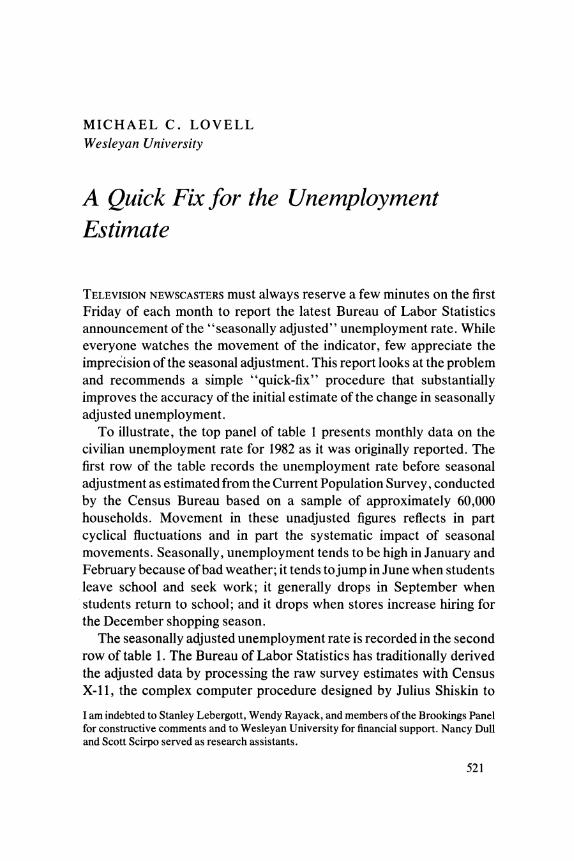
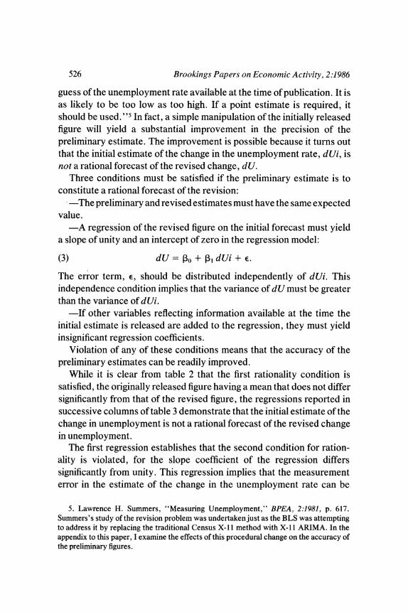
To illustrate, the top panel of table 1 presents monthly data on the civilian unemployment rate for 1982 as it was originally reported. The first row of the table records the unemployment rate before seasonal adjustment as estimated from the Current Population Survey, conducted by the Census Bureau based on a sample of approximately 60,000 households. Movement in these unadjusted figures reflects in part cyclical fluctuations and in part the systematic impact of seasonal movements. Seasonally, unemployment tends to be high in January and February because of bad weather; it tends to jump in June when students leave school and seek work; it generally drops in September when students return to school; and it drops when stores increase hiring for the December shopping season.

The seasonally adjusted unemployment rate is recorded in the second row of table 1. The Bureau of Labor Statistics has traditionally derived the adjusted data by processing the raw survey estimates with Census X-1 1, the complex computer procedure designed by Julius Shiskin to

I am indebted to Stanley Lebergott, Wendy Rayack, and members of the Brookings Panel for constructive comments and to Wesleyan University for financial support. Nancy Dull and Scott Scirpo served as research assistants.

521

O; oo o so oo

o t~~~~~~~~~~~~~~~~~~~~~~~~~~6 00 t<tboY?C

b t e N

~~~~~~~~~~~~~~~~~~o s c

00 ? 00 N N O o ? S Y~~~~~~~~~~~~~~~~~~~~~~~~~~~~~~~0

$ 00 00 0 0 e 00 N O C1, 0~~~~~~~~~~~~0

~~~~~~N S0 oo c en O ?N en =C

> o o O O O o O O O Q = S~~~~~~~~ 0

w~~~~~~~~~~~~~~~Q 0 (t. - o 0 n

t o U3 ? 4X

<)~ ~~~~~~~~~~~~~Q In In I YY

;~~~~~~~~~~~~~~~Q D . ut S D: ? Ci6-

: > I I D>E?z->~~~~~~~~~M

F* A4 X4 u C4 u dc

Michael C. Lovell 523

filter out typical seasonal variation and yield data that capture more accurately underlying cyclical and trend movements.' The seasonal adjustment, the adjusted rate less the unadjusted rate, is recorded on the third row of the table. At times the unadjusted figures dance in a quite different way from the adjusted series, as in June when the unadjusted figure increased by 0.7 percentage point at the end of the school year while the adjusted rate held steady. It is usually the change in the adjusted unemployment rate, reported on the fifth line of the table, rather than the level of unemployment, that grabs the headlines.

The Bureau of Labor Statistics recalculates the seasonal adjustment factors each year for five years. With the aid of hindsight the BLS can reestimate with greater precision the customary seasonal movement and get a more precise estimate of the seasonally adjusted unemployment rate. For example, knowing how unemployment fluctuated seasonally in 1983, 1984, and 1985 helps in estimating the appropriate seasonal corrections for 1982. The most recently revised estimates of the level and month-to-month change in unemployment for 1982 are recorded in the two rows in the center panel of table 1. The bottom panel of the table reports the revisions gotten by subtracting the initial figure from the latest available estimate. While many of the revisions are small, some are startlingly large: the December 1981 seasonally adjusted rate, initially reported to be 8.9 percent, is now estimated to have been 8.5 percent. Thus the decline in unemployment for January 1982, so encouraging when reported at the beginning of February, turns out to have been a bogus dip. It should be noted that the latest estimates recorded in table 1 are not final; they will be subject to a fifth and final annual revision in January of 1987. When economic historians look back on what happened to the American economy when it slid into the most severe recession since World War II, they will be privileged to study economic conditions in 1982 from a different and more accurate perspective than that provided at the time to policymakers and economic decisionmakers.

The next section of this report presents descriptive statistics reviewing the extent of the revision problem. The third section shows that the initial estimate of the change in the unemployment rate is subject to

1. See Julius Shiskin and Harry Eisenpress, "Seasonal Adjustments by Electronic Computer Methods," Journal of the American Statistical Association, vol. 52 (December 1957), pp. 415-49.

524 Brookings Papers on Economic Activity, 2:1986

systematic error. As a result, a considerable gain in accuracy can be obtained simply by reducing the initially reported change in the unem- ployment rate by a factor of one-third. Slightly more involved adjustment procedures lead to additional precision and a reduction in erratic fluc- tuations.

Summary Statistics

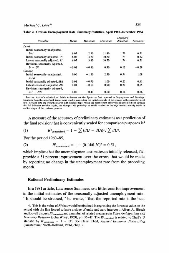
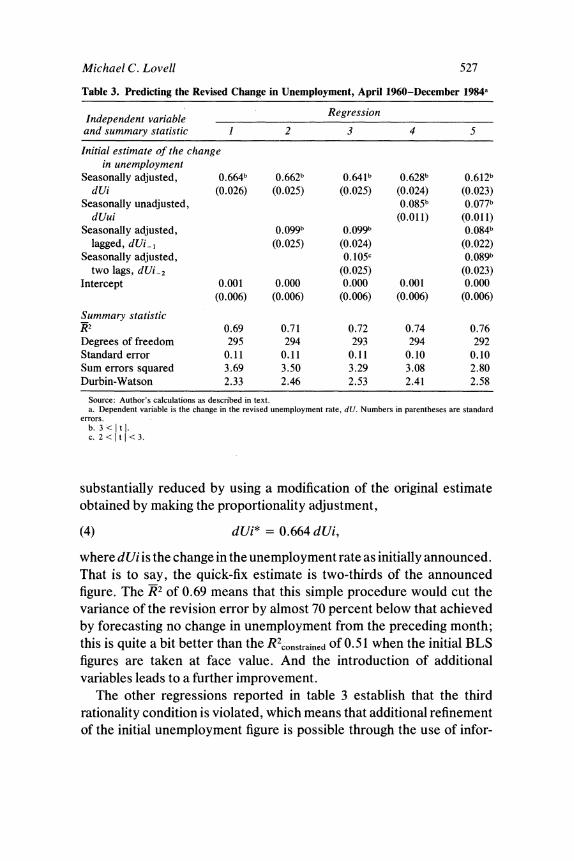
Table 2 contrasts the initially announced seasonally adjusted monthly unemployment rates from 1960 to 1984 with the latest available estimates for those dates. Observe that the latest series, U, and the initially announced data, Ui, have essentially the same mean and variance. But as can be seen from the fourth row of the table, the revision, U - Ui, has at times been quite substantial, ranging from -0.4 percent to 0.3 percent. Of even greater interest is the gap between the revised and the initial estimate of the month-to-month change in the unemployment rate, dU - dUi, which has ranged from - 0.4 percent to 0.6 percent. All the variables are symmetrically distributed, except the change in the unad- justed unemployment rate, dUui, which is skewed to the right. The distribution of change revisions is approximately normal, with 22 percent of the revisions of the month-to-month change larger in absolute value than 0.1 percentage point.

The standard deviation of the revision error for month-to-month changes, dU - dUi, is 0.14 percent, or about half the 0.25 percent standard deviation of the initially reported change in unemployment, dUi; that is to say, a substantial share of the movement that the public reacts to in the unemployment rate is "noise. ' 2 The fact that the standard deviation of the initial estimate of the change in unemployment is greater than that of the revisions means that there is bogus bounce in the initial announcements of unemployment rate changes.3 In light of these sub- stantial errors, it would seem appropriate for the Bureau of Labor Statistics to attach the label "preliminary" to the unemployment rate estimates they announce each month.

2. In terms of the vocabulary of electrical engineers, there is a "signal to signal plus noise ratio" of 76 percent = variance of U/[variance of U + variance of (U - Ui)].

3. Since the initial announcements have greater variance than the revisions, they cannot be rational forecasts of the revisions. The quick-fix procedure explained later in this paper controls the bogus bounce.

Michael C. Lovell 525

Table 2. Civilian Unemployment Rate, Summary Statistics, April 1960-December 1984

Standard Variable Mean Minimum Maximum deviation Skewness

Level Initial seasonally unadjusted,

Uui 6.07 2.90 11.40 1.79 0.51 Initial seasonally adjusted, Ui 6.08 3.30 10.80 1.73 0.52 Latest seasonally adjusted, U 6.07 3.40 10.70 1.74 0.51 Revision, seasonally adjusted,

U - Ui -0.01 -0.40 0.30 0.12 -0.28 Change

Initial seasonally unadjusted, 0.00 -1.10 2.30 0.54 1.08 dUui

Initial seasonally adjusted, dUi 0.01 -0.70 1.00 0.25 0.41 Latest seasonally adjusted, dU 0.01 -0.70 0.90 0.20 0.55 Revision, seasonally adjusted,

dU - dUi 0.00 -0.40 0.60 0.14 0.56

Sources: Author's calculations. Initial estimates are the figures as first reported in Employment and Earnings. Numbers from the same back issues were used in computing the initial estimate of the change in the unemployment rate. Revised data are from the March 1986 Citibase tape. While the most recent observations have not been through the full five-year revision cycle, the changes will probably be small relative to the adjustments already made in earlier stages of the revision process.

A measure of the accuracy of preliminary estimates as a prediction of the final revision that is conveniently scaled for comparison purposes iS4

(1) R2constrained = 1 -I (dU - dUi)2 / , dC]2.

For the period 1960-85,

(2) R2 constrained = 1 - (0.14/0.20)2 = 0.51,

which implies that the unemployment estimates as initially released, Ui, provide a 51 percent improvement over the errors that would be made by reporting no change in the unemployment rate from the preceding month.

Rational Preliminary Estimates

In a 1981 article, Lawrence Summers saw little room for improvement in the initial estimates of the seasonally adjusted unemployment rate. "It should be stressed," he wrote, "that the reported rate is the best

4. This is the value of R2 that would be obtained in regressing the forecast value on the actual with the line forced to have a slope of unity and zero intercept. Albert A. Hirsch and Lovell discuss R2constrained and a number of related measures in Sales Anticipations and Inventory Behavior (John Wiley, 1969), pp. 35-42. The R2constrained is related to Theil's U statistic by R2constrained = 1 - U2. See Henri Theil, Applied Economic Forecasting (Amsterdam: North-Holland, 1966), chap. 2.

526 Brookings Papers on Economic Activity, 2:1986

guess of the unemployment rate available at the time of publication. It is as likely to be too low as too high. If a point estimate is required, it should be used. "5 In fact, a simple manipulation of the initially released figure will yield a substantial improvement in the precision of the preliminary estimate. The improvement is possible because it turns out that the initial estimate of the change in the unemployment rate, dUi, is not a rational forecast of the revised change, dU.

Three conditions must be satisfied if the preliminary estimate is to constitute a rational forecast of the revision:

-The preliminary and revised estimates must have the same expected value.

-A regression of the revised figure on the initial forecast must yield a slope of unity and an intercept of zero in the regression model:

(3) dU = 0 + P1 dUi+ E.

The error term, E, should be distributed independently of dUi. This independence condition implies that the variance of dU must be greater than the variance of dUi.

-If other variables reflecting information available at the time the initial estimate is released are added to the regression, they must yield insignificant regression coefficients.

Violation of any of these conditions means that the accuracy of the preliminary estimates can be readily improved.

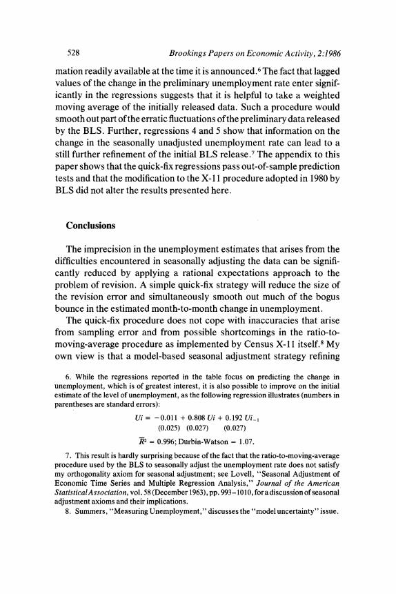
While it is clear from table 2 that the first rationality condition is satisfied, the originally released figure having a mean that does not differ significantly from that of the revised figure, the regressions reported in successive columns of table 3 demonstrate that the initial estimate of the change in unemployment is not a rational forecast of the revised change in unemployment.

The first regression establishes that the second condition for ration- ality is violated, for the slope coefficient of the regression differs significantly from unity. This regression implies that the measurement error in the estimate of the change in the unemployment rate can be

5. Lawrence H. Summers, "Measuring Unemployment," BPEA, 2:1981, p. 617. Summers's study of the revision problem was undertaken just as the BLS was attempting to address it by replacing the traditional Census X-1 1 method with X-1 1 ARIMA. In the appendix to this paper, I examine the effects of this procedural change on the accuracy of the preliminary figures.

Michael C. Lovell 527

substantially reduced by using a modification of the original estimate obtained by making the proportionality adjustment,

(4) dUi* = 0.664 dUi,

where dUi is the change in the unemployment rate as initially announced. That is to say, the quick-fix estimate is two-thirds of the announced figure. The R2 of 0.69 means that this simple procedure would cut the variance of the revision error by almost 70 percent below that achieved by forecasting no change in unemployment from the preceding month; this is quite a bit better than the R2constrained of 0.51 when the initial BLS figures are taken at face value. And the introduction of additional variables leads to a further improvement.

The other regressions reported in table 3 establish that the third rationality condition is violated, which means that additional refinement of the initial unemployment figure is possible through the use of infor-

Table 3. Predicting the Revised Change in Unemployment, April 1960-December 1984a

Independent variable Regression and summary statistic 1 2 3 4 5

Initial estimate of the change in unemployment

Seasonally adjusted, 0.664b 0.662b 0.641b 0.628b 0.612b dUi (0.026) (0.025) (0.025) (0.024) (0.023)

Seasonally unadjusted, 0.085b 0.077b dUui (0.011) (0.011)

Seasonally adjusted, 0.099b 0.099b 0.084b

lagged, dUi-l (0.025) (0.024) (0.022) Seasonally adjusted, 0. 105c 0.089b

two lags, dUi-2 (0.025) (0.023) Intercept 0.001 0.000 0.000 0.001 0.000

(0.006) (0.006) (0.006) (0.006) (0.006)

Summary statistic K2 0.69 0.71 0.72 0.74 0.76 Degrees of freedom 295 294 293 294 292 Standard error 0.11 0.11 0.11 0.10 0.10 Sum errors squared 3.69 3.50 3.29 3.08 2.80 Durbin-Watson 2.33 2.46 2.53 2.41 2.58

Source: Author's calculations as described in text. a. Dependent variable is the change in the revised unemployment rate, dU. Numbers in parentheses are standard

errors. b. 3 < It c. 2 < t < 3.

528 Brookings Papers on Economic Activity, 2:1986

mation readily available at the time it is announced.6 The fact that lagged values of the change in the preliminary unemployment rate enter signif- icantly in the regressions suggests that it is helpful to take a weighted moving average of the initially released data. Such a procedure would smooth out part of the erratic fluctuations of the preliminary data released by the BLS. Further, regressions 4 and 5 show that information on the change in the seasonally unadjusted unemployment rate can lead to a still further refinement of the initial BLS release.7 The appendix to this paper shows that the quick-fix regressions pass out-of-sample prediction tests and that the modification to the X-1 1 procedure adopted in 1980 by BLS did not alter the results presented here.

Conclusions

The imprecision in the unemployment estimates that arises from the difficulties encountered in seasonally adjusting the data can be signifi- cantly reduced by applying a rational expectations approach to the problem of revision. A simple quick-fix strategy will reduce the size of the revision error and simultaneously smooth out much of the bogus bounce in the estimated month-to-month change in unemployment.

The quick-fix procedure does not cope with inaccuracies that arise from sampling error and from possible shortcomings in the ratio-to- moving-average procedure as implemented by Census X-1 1 itself.8 My own view is that a model-based seasonal adjustment strategy refining

6. While the regressions reported in the table focus on predicting the change in unemployment, which is of greatest interest, it is also possible to improve on the initial estimate of the level of unemployment, as the following regression illustrates (numbers in parentheses are standard errors):

Ui =-0.011 + 0.808 Ui + 0.192 Uil (0.025) (0.027) (0.027)

R2 = 0.996: Durbin-Watson = 1.07.

7. This result is hardly surprising because of the fact that the ratio-to-moving-average procedure used by the BLS to seasonally adjust the unemployment rate does not satisfy my orthogonality axiom for seasonal adjustment; see Lovell, "Seasonal Adjustment of Economic Time Series and Multiple Regression Analysis," Journal of the American StatisticalAssociation, vol. 58 (December 1963), pp. 993 -1010, for a discussion of seasonal adjustment axioms and their implications.

8. Summers, "Measuring Unemployment," discusses the "model uncertainty" issue.

Michael C. Lovell 529

the least-squares procedure would yield a substantial improvement over the traditional ratio-to-moving-average strategy embodied in Census X- 11.9 In the spirit of rational expectations, analysts should be explicitly modeling the process by which seasonal fluctuations are generated, incorporating monthly data on such variables as school enrollments, weather conditions, and seasonal hiring trends.

APPENDIX

X-11 ARIMA

THE Bureau of Labor Statistics addressed the revision error problem in 1980 by modifying the Census X-1 1 seasonal adjustment program tradi- tionally employed for filtering seasonal fluctuations out of the unemploy- ment data. As explained in greater detail by Robert J. McIntire, the modified X-1 1 ARIMA procedure, developed by Estela Bee Dagum of Statistics Canada, attempts to circumvent the "end-point" problem by using a two-step procedure: first, the Auto-Regressive-Integrated-Mov- ing-Average (ARIMA) technique is used to extrapolate the observed unadjusted time series for an additional year into the future; second, Census X- 11 is applied directly to the artificially extended time series. 10 Further, instead of computing the seasonal adjustment factors to be used for the coming year each January, the BLS now computes six-month lead time factors in January and June. " I

9. Michael C. Lovell, "Least-Squares Seasonally Adjusted Unemployment Data," BPEA, 1:1976, pp. 225-37.

10. RobertJ. Mclntire, "Revision of Seasonally Adjusted Labor Series," Employment and Earnings, vol. 33 (January 1986), pp. 9-11.

11. The BLS has traditionally announced seasonal adjustment factors in advance in order to avoid any suggestion that the figures are fudged; starting in 1980 the adjustment factors are announced six months in advance. For example, the seasonal adjustment factors to be used in adjusting the unemployment rates for the first half of 1982 were computed on the basis of data through December of 1981. The bureau has been contem- plating a shift to "Concurrent Adjustment," which involves computing the factors each month on the basis of all the available historical evidence. The bureau obtains the seasonally adjusted aggregate unemployment rate by aggregating the results obtained by applying Census X- 11 separately to labor force and employment data for twelve demographic groups.

530 Brookings Papers on Economic Activity, 2:1986

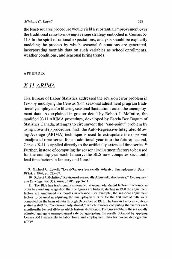
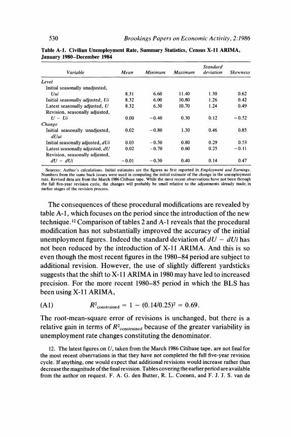
The consequences of these procedural modifications are revealed by table A- 1, which focuses on the period since the introduction of the new technique.'2 Comparison of tables 2 and A- 1 reveals that the procedural modification has not substantially improved the accuracy of the initial unemployment figures. Indeed the standard deviation of dU - dUi has not been reduced by the introduction of X- 11 ARIMA. And this is so even though the most recent figures in the 1980-84 period are subject to additional revision. However, the use of slightly different yardsticks suggests that the shift to X- 11 ARIMA in 1980 may have led to increased precision. For the more recent 1980-85 period in which the BLS has been using X- 11 ARIMA,

(Al) R2constrained = 1 - (0.14/0.25)2 = 0.69.

The root-mean-square error of revisions is unchanged, but there is a relative gain in terms of R2constrained because of the greater variability in unemployment rate changes constituting the denominator.

Table A-1. Civilian Unemployment Rate, Summary Statistics, Census X-11 ARIMA, January 1980-December 1984

Standard Variable Mean Minimum Maximum deviation Skewness

Level Initial seasonally unadjusted,

Uui 8.31 6.60 11.40 1.30 0.62 Initial seasonally adjusted, Ui 8.32 6.00 10.80 1.26 0.42 Latest seasonally adjusted, U 8.32 6.30 10.70 1.24 0.49 Revision, seasonally adjusted,

U - Ui 0.00 -0.40 0.30 0.12 -0.52 Change

Initial seasonally unadjusted, 0.02 -0.80 1.30 0.46 0.85 dUui

Initial seasonally adjusted, dUi 0.03 - 0.50 0.80 0.29 0.53 Latest seasonally adjusted, dU 0.02 -0.70 0.60 0.25 -0.11 Revision, seasonally adjusted,

dU - dUi -0.01 -0.30 0.40 0.14 0.47

Sources: Author's calculations. Initial estimates are the figures as first reported in Employment and Earnings. Numbers from the same back issues were used in computing the initial estimate of the change in the unemployment rate. Revised data are from the March 1986 Citibase tape. While the most recent observations have not been through the full five-year revision cycle, the changes will probably be small relative to the adjustments already made,,in earlier stages of the revision process.

12. The latest figures on U, taken from the March 1986 Citibase tape, are not final for the most recent observations in that they have not completed the full five-year revision cycle. If anything, one would expect that additional revisions would increase rather than decrease the magnitude of the final revision. Tables covering the earlier period are available from the author on request. F. A. G. den Butter, R. L. Coenen, and F. J. J. S. van de

Michael C. Lovell 531

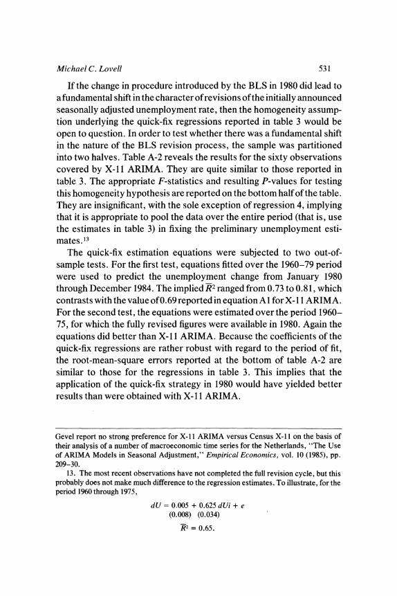
If the change in procedure introduced by the BLS in 1980 did lead to a fundamental shift in the character of revisions of the initially announced seasonally adjusted unemployment rate, then the homogeneity assump- tion underlying the quick-fix regressions reported in table 3 would be open to question. In order to test whether there was a fundamental shift in the nature of the BLS revision process, the sample was partitioned into two halves. Table A-2 reveals the results for the sixty observations covered by X-1 1 ARIMA. They are quite similar to those reported in table 3. The appropriate F-statistics and resulting P-values for testing this homogeneity hypothesis are reported on the bottom half of the table. They are insignificant, with the sole exception of regression 4, implying that it is appropriate to pool the data over the entire period (that is, use the estimates in table 3) in fixing the preliminary unemployment esti- mates. 13

The quick-fix estimation equations were subjected to two out-of- sample tests. For the first test, equations fitted over the 1960-79 period were used to predict the unemployment change from January 1980 through December 1984. The implied R2 ranged from 0.73 to 0.81, which contrasts with the value of 0.69 reported in equation A l for X- 11 ARIMA. For the second test, the equations were estimated over the period 1960- 75, for which the fully revised figures were available in 1980. Again the equations did better than X-1 1 ARIMA. Because the coefficients of the quick-fix regressions are rather robust with regard to the period of fit, the root-mean-square errors reported at the bottom of table A-2 are similar to those for the regressions in table 3. This implies that the application of the quick-fix strategy in 1980 would have yielded better results than were obtained with X- 1I ARIMA.

Gevel report no strong preference for X- 11 ARIMA versus Census X- 11 on the basis of their analysis of a number of macroeconomic time series for the Netherlands, "The Use of ARIMA Models in Seasonal Adjustment," Empirical Economics, vol. 10 (1985), pp. 209-30.

13. The most recent observations have not completed the full revision cycle, but this probably does not make much difference to the regression estimates. To illustrate, for the period 1960 through 1975,

dU = 0.005 + 0.625 dUi + e (0.008) (0.034)

W2 = 0.65.

532 Brookings Papers on Economic Activity, 2:1986

Table A-2. Rational Preliminary Data Regressions, ARIMA Subperiod, January 1980-December 1984a

Independent variable and Regression summary statistic 1 2 3 4 5

Initial estimate of the change in unemployment

Seasonally adjusted, 0.751 b 0.698b 0.697b 0.700b 0.679b dUi (0.054) (0.055) (0.055) (0.045) (0.047)

Seasonally unadjusted, 0.152b 0.136b dUui (0.028) (0.030)

Seasonally adjusted, 0.146c 0.125c 0.068 lagged, dUi-l (0.055) (0.058) (0.051)

Seasonally adjusted, 0.059 0.015 two lags, dUi-2 (0.055) (0.048)

Intercept 0.000 -0.003 -0.003 -0.002 -0.003 (0.015) (0.015) (0.015) (0.013) (0.013)

Summary statistic R2 0.77 0.79 0.79 0.84 0.84 Degrees of freedom 58 57 56 57 55 Standard error 0.12 0.11 0.11 0.10 0.10 Sum errors squared 0.81 0.72 0.71 0.54 0.52 F-statisticd 2.42 1.12 0.66 3.93 1.90 P-value (percent)d 8.9 34.0 61.7 0.9 9.3 Root-mean-square error,

1980-84 Equation fit to 1960-80 0.128 0.122 0.121 0.114 0.110 Equation fit to 1960-75 0.131 0.124 0.123 0.116 0.129

Source: Author's calculations as described in text. a. Dependent variable is the change in the revised unemployment rate, dU. Numbers in parentheses are standard

errors. b. 3 < It I. c. 2 < t I<3. d. The F-statistic and the P-value rows report the results of the test that there was no shift in the underlying

structure as a result of the change to X-1 I ARIMA in 1980.

Comments and Discussion

William Brainard questioned whether most observers were seriously misled by the initial estimates of the month-to-month change in the unemployment rate. His impression was that many forecasters dis- counted the newly released data in a fashion not inconsistent with what Lovell would argue is rational. William Poole noted that the BLS releases alternative estimates of the seasonally adjusted unemployment rate each month, each constructed by a different procedure. Although these estimates obviously receive less attention than the official numbers, they warn users against attaching too much precision to any one number. Richard Cooper suggested that the only way to reduce the attention paid to the initial estimates of the unemployment rate would be to hold up their release until they were no longer news.

Christopher Sims argued that it was appropriate for the BLS to make its procedures mechanical and transparent. With model-based seasonal adjustment, each series would have a different univariate model, and these models would change every few years. The BLS would have to publish a large book just to describe the models used. Sims's concern was less whether the BLS's seasonal adjustment procedure is optimal than whether it is standardized in a way that avoids subjective adjust- ments.

Sims also wondered how much of the irrationality in the initial estimates of the seasonally adjusted unemployment rate could be attrib- uted to the fact that the seasonal adjustment factors are fixed six months ahead of time. Poole noted that an alternative to Lovell's "quick fix" would be to rerun the Census X- 11 program and generate new seasonal adjustment factors every month, rather than using seasonal factors that were fixed ahead of time; but he conceded that it would be difficult to

533

534 Brookings Papers on Economic Activity, 2:1986

explain to the public why this month's unemployment rate should affect last month's unemployment rate. Thomas Plewes, Associate Commis- sioner of the BLS, reported that the bureau is currently considering using concurrent seasonal adjustment as described by Poole. Such a change, he said, would eliminate the need for Lovell's "quick-fix" procedure.

Martin Baily pointed out that the paper assumes that the final seasonally adjusted numbers are correct, whereas in fact they may not be. The Census X-1 1 procedure puts a heavy weight on the current year in estimating seasonal factors. For example, if a recession starts in January, the seasonal adjustment procedure will attribute part of that month's employmentweakness to seasonalfactors and thus may produce too low a seasonally adjusted unemployment rate for that January. More generally, the Census X- 11 procedure removes from the data not only true seasonal components but also variation from other sources, so that in a sense it overadjusts. Sims observed that apparent overadjustment would inevitably characterize an optimally adjusted series, in the sense that it should have less variance than either the unadjusted raw series or the unobservable underlying nonseasonal component. Thus, he argued, it is not necessarily a defect in the BLS procedures that they result in such apparent overadjustment.