1

Field initializing equation numbering variables here: November 7, 2013; December 4, 2016; June 25, 2018

DRAFT

Chapter from the Material Theory of Induction.

AQuantumInductiveLogicJohn D. Norton

Department of History and Philosophy of Science

University of Pittsburgh

http://www.pitt.edu/~jdnorton

1.Introduction1 The material theory of induction requires that good inductive inferences must be

warranted by facts within their domain of application. In earlier chapters, we have seen many

examples of individual inductive inferences warranted by specific facts. Marie Curie, for

example, inferred the crystallographic system of all crystals of radium chloride from inspection

of just a few specks of the substance. The inference was warranted by facts contained in

crystallographic principles from the preceding century, not by some universal inductive inference

schema.

In cases like this, there is little sense that the inductive inference forms part of a larger

inductive logic whose overall structure could be abstracted in some measure from the specific

subject matter. There are cases, however, in which this abstraction is possible. Complete

abstraction is impossible; that would provide a universal logic of induction. We can find cases in

which sufficient structure can be abstracted for a rich logic to appear.

The most familiar inductive logic of this type and the one that is best worked out is that

of probabilistic logic. The prevalence of this probabilistic logic has given the illusion that it is the

universal inductive logic and that no other inductive logic is viable. That illusion persists only

because of the familiarity of the example and the lack of looking for alternatives. If we have any

1 I thank Rob Spekkens for helpful discussion.

2

domain governed by some well-developed theory, then a compactly expressible inductive logic

may be supported. Just which that logic will be, depends on the character of the theory. There

will be cases in which the logic supported is not probabilistic.

In the preceding chapters, such cases were illustrated with simple examples: an infinite

lottery machine, various forms of indeterministic systems and the non-measurable outcomes

arising among infinitely many coin tosses. While we can and should demand that an inductive

logic applies to these cases, one can be forgiven for finding the examples contrived or abstruse.

They were so precisely because that enabled the systems to be simple enough for us to

comprehend their physical properties fully.

Might we find an example with an immediate application to present science? This chapter

presents such an example. Drawing on the work of Leifer and Spekkens (2013), we shall see that

the natural mathematical structures of quantum theory afford a distinctive, non-probabilistic

logic, at least for certain quantum systems, such as systems of entangled particles.

This quantum inductive logic differs from a probabilistic inductive logic in its most

fundamental quantity. A probabilistic logic uses an additive probability measure to represent

degrees of support or, in subjective terms, belief states. In its place, the quantum logic uses a

structure that arises naturally in quantum theory, a density operator. That this is the appropriate

structure derives in turn from a deeper difference. Probabilities arise naturally when all of the

distinct states of a system fall under a single probability measure supplied by background facts.

While there are probabilities associated with measurement outcomes in quantum theory, each

measurement setting is associated with a different probability measure and, crucially, their

totality does not form a single probability measure. Rather the different probability measures are

both issued by and unified by a single, deeper structure, a density operator. That structure is the

fundamental quantity of the quantum inductive logic.

It may seem strange at first to replace a probability measure by a density operator when

probabilities can also be found in quantum theory, even if in scattered form. For, one might

think, a probability measure, when it can be had, is just the right thing to use to represent partial

inductive support or uncertain beliefs. This thought is driven more by familiarity and comfort

than good reasons. The naturalness of a probability measure is an artifact of hundreds of years of

development. It is a rather abstruse notion, as one finds when one engages in the cumbersome

task of explicating precisely what it means to say that, for example, some outcome has such and

3

such a probability. We shall see below that a density operator is no more abstruse and, since it is

the central structure provided by the quantum mechanics, it functions much better as the basis of

the quantum inductive logic.

Section 2 below will sketch some probabilistic inferences on the presence of a rare

genetic mutation among siblings. It will serve as a foil for the quantum case introduced in

Sections 3 and 4, inductive inferences over the measured spins of entangled electrons. Section 5

to 9 develop the mathematical devices needed to treat the spins of entangled electrons. Sections

10 and 11 will identify one of these devices, a density operator, as the appropriate analog in the

quantum case of the probabilities of the foil. Section 12 will provide a simple geometric picture

of the density operators to support this identification. Section 13 will briefly review how Leifer

and Spekkens (2013) have developed the approach sketched into a fuller calculus with some

analogies to the probability calculus. Sections 14 and 15 explore analogies and disanalogies

between the probabilistic and quantum inductive logics. Section 16 offers conclusions.

2.ProbabilisticInductiveInference

2.1RareGeneticMutations

As a foil for the quantum case, let us consider cases in which a probabilistic logic is

warranted by the prevailing facts. One arises when we have outcomes generated by physical

chances. The simplest of these is a gambling casino. By careful design, a roulette wheel (with a 0

and 00) has a physical chance of 18/38 of a red outcome; and a physical chance of 18/38 of a

black outcome. That fact, and others like it, warrant using the corresponding probabilities as the

measure of inductive support for red and black; and employing the probability calculus as the

logic of induction applicable to casino games.

Population frequencies can also provide a factual warrant for the use of probabilities in an

inductive logic. Demographic data consistently shows that low educational level correlates with

unemployment. People in the US without a high school diploma, for example, are the group with

the most unemployment. We make the added assumption that some individual has been chosen

randomly, where randomly just means that each individual in the population has an equal

probability of being chosen. It follows that the probability that the individual selected has a

certain property matches the frequency of the property in the population. We can then use these

4

probabilities as the measures of inductive support for the propositions that the individual has

various educational levels and various employment statuses. That the individual has no high

school diploma increases the inductive support for the proposition that the individual is

unemployed; for the probability of unemployment given no high school diploma is greater than

the unconditioned probability of unemployment.

Inductive inferences concerning genetic mutations in some population combine the

essential features of the last two cases. To make matters concrete, consider a human population

in which a mutation of some particular gene arises, but only very rarely. To make the example

more interesting, assume that the mutation can arise in n mutually exclusive variations, so we

have possible alleles

N, m1, …, mn

where N is the overwhelmingly most common case of no mutation—hence the symbol N for

“No.” We have a population of alleles in which the n mutations will arise with varying

frequency. Physical chance process will govern the propagation of the alleles through the

generations and those physical chances will determine the equilibrium distribution frequency of

the various alleles. If standard, idealized conditions are met, these frequencies will conform with

the Hardy-Weinberg equilibrium.

2.2InductiveInferenceProblems

The conditions just specified are the background facts that warrant inductive inferences

over the presence of the mutation in the population. Since the physical chances are probabilistic,

these inferences will be within a probabilistic inductive logic.

Consider some randomly selected child. The fact of random selection means that the

probability that the child carries mutation mi matches the overall frequency ri of mutation-i

carrying individuals in the population. These facts together warrant our use of probabilities as the

measure of inductive support, where those probabilities are matched with population frequencies.

5

Consider two sibling children in some family. The measures of inductive support that

each carries the mutation mi is given by the two probability measures:2

P(child1 carries mi) = ri << 1 i=1,…,n (1)

P(child2 carries mi) = ri << 1 i=1,…,n

These two probabilities must also be related by the rule of total probability:

P(child2 carries mi)

= P(child2 carries mi | child1 carries mi) . P(child1 carries mi)

+ P(child2 carries mi | not-child1 carries mi) . P(not-child1 carries mi) (2)

In general, the two conditional probabilities in this last formula are quite complicated

expressions of the various gene frequencies. However, for the case of extremely rare mutations,

that is ri << 1, they are approximated very well by

P(child2 carries mi | child1 carries mi) = 1/2

P(child2 carries mi | not-child1 carries mi) = ri

2(1-ri) (3)

The first conditional probability arises from the circumstance that, if child1 carries mi, then it is

overwhelmingly likely that just one of the children’s parents carries mutation mi. It is possible

that a parent may carry two copies, or both parents may carry copies, but these cases are vastly

less likely and can be neglected. If just one of the children’s parents carries mutation mi, then

there is a probability of 1/2 that child2 inherits it. The second conditional is recovered from a

short application of Bayes’ theorem.3

2 More exactly, if the allele carrying the mutation mi arises with frequency fi in the population

and the gene distribution has arrived at the Hardy-Weinberg equilibrium, then the probability

that the child carries one or both of the mutated alleles is ri = 2 fi(1- fi) + fi2 ≈ 2fi for small fi<<1.

3 Writing c1 = child1 carries mi and c2 = child2 carries mi, we have from Bayes’ theorem that

P(c2 | not-c1) = P(not-c1 | c2)

P(not-c1) P(c2) = (1/2)ri/(1-ri)

since P(c2) = ri , P(not-c1) = (1- ri) and P(not-c1 | c2) = 1 - P(c1 | c2) ≈ 1-1/2 = 1/2.

6

We can use the conditional probabilities (3) to support an inference from the probability

that child1 carries mi to the probability that child2 carries mi. Substituting (3) into (2) we find:

P(child2 carries mi)

= 1/2 . P(child1 carries mi) + ri

2(1-ri) . P(not-child1 carries mi)

= 1/2 ri + ri

2(1-ri) (1- ri) = ri = P(child1 carries mi) (4)

which agrees with (1).

This last inference is a particular case of how the rule of total probability becomes a rule

of inductive inference in the probabilistic logic. Consider an outcome space that can be

partitioned into mutually exclusive outcomes in two ways; that is as {S0, S1, … , Sn} and as {R0,

R1, … , Rn}. We start with the probability distribution P(Rk) for k=0, … , n as representing the

inductive support for the outcomes Rk. The conditional probabilities P(Si | Rk) for i,k = 0, …, n,

allow us to infer from the support accrued to the outcomes Bk to the support accrued to the

outcomes Ai, by means of the rule of total probability:

P(Si) = ΣkP(Si | Rk) P(Rk) (5)

3.FromMutationstoElectrons Quantum mechanics describes a physical realm that differs from those of more familiar

systems in which probabilistic logics are appropriate. The facts that comprise quantum theory

can warrant a rather different inductive logic for certain quantum systems. One of these systems,

a pair of entangled particles, is analogous to the pairs of children of the mutation case above in

that it is comprised of two related systems. However if we try to carry out inductive inferences

analogous to those concerning mutations carried by children, we will find that we need to use a

non-probabilistic inductive logic and that this logic can be read off directly from the quantum

mechanical formalism.

7

This is not the place to attempt a self-contained development of the standard formalism of

quantum theory.4 However my concern is that the development is accessible to those who do not

work in quantum theory. I will do my best to motivate and explain the least amount needed to

convey the main ideas to you, if you have less familiarity with the formalism. So do keep

reading—this is written for you.

In the following, we will consider one of the simplest properties of one of the simplest,

best-known particles. That is, we will consider electrons and their spins. Electrons carry angular

momentum. Classically, angular momentum is a measure of the quantity of rotational motion of

a body like a spinning top. It is the rotational analog of ordinary linear momentum—“mass time

velocity”—and, for the spinning top, is “moment of inertia times the angular velocity.” It is a

vector quantity and is fully specified when we have fixed its real number magnitude and its

direction in space. The magnitude is determined by the speed of rotation and the mass

distribution in the top, as expressed by its moment of inertia. The direction is fixed by the axis of

rotation.5 Angular momentum acquires its importance in both classical and quantum systems

since it is a conserved quantity. The total angular momentum remains constant in all closed

interactions.

It is almost the same with the spin of the electron. The angular momentum of the electron

has a magnitude. Unlike a classical top that can spin faster and slower and thus can carry more or

less angular momentum, all electrons carry the same magnitude of spin angular momentum. It is

1/2 in units of h/2π (where h is Planck’s constant). Since it is the same for all electrons, this

magnitude is unimportant for what follows. Like the top, electron spin also has a direction and

this direction can take all orientations in space. That direction is the quantity that will interest us.

That direction is what is measured in many foundational thought experiments in quantum

mechanics.

4 To fill in the inevitable technical gaps, an account such as Nielsen and Chuang (2010, Ch. I)

can be consulted. 5 Which direction along the axis? Up or down? The right hand rule tells us that, if the direction

of rotation follows the direction of the curled fingers of the right hand, then the hand’s upright

thumb indicates the direction.

8

The major disanalogy between spinning tops and electrons with spin is that there is

nothing rotating or spinning inside the electron. An electron carries angular momentum in the

same way that it carries electric charge, as a fundamental, irreducible property. There is no

deeper story about some hidden, spinning machinery that explains how the angular momentum

comes about. It is just there.

4.TwoInductiveInferenceProblemsforElectrons The background facts fix the inductive logic appropriate to some domain. We can find

situations involving electrons in which a familiar probabilistic induction is the appropriate one;

and we can find situations in which it is not.

4.1UncertaintyoverRandomlySelectedStates

Here is an example of the first. Electrons can have spins that point in all directions.

Imagine that we have prepared many (unentangled) electrons whose spin directions are

uniformly distributed over all directions. One—we know not which—is selected. On the

evidence of this set up, how much inductive support is accrued to each possible spin direction?

This is almost a problem that calls for a probabilistic logic. What is missing are facts that would

require this logic. They are easily supplied. We add to the set up that the selection is random,

where this means that each candidate electron has an equal probability of selection. It then

follows that each spin direction is equally probable for the electron selected and thus equally

well supported.

A probabilistic inductive logic is warranted by the set up, for in it all possible outcomes

fall under a single probability measure. No quantum peculiarity has entered. The analysis would

be the same if, instead of electrons, we had prepared many classical arrows, pointing in different

directions, and selected one randomly.

4.2UncertaintyoverMeasurementsonElectronsinEntangledStates

Now consider a second problem. It is possible to entangle two electrons so that their

states are highly correlated. In the simplest case of two electrons in a singlet state (to be

explained below), the two electrons have spins that always point in opposite directions. If one is

measured to have a spin that points North, the other will always be measured to point South; and

9

so on for every other possible pairing of opposite directions. This singlet state can persist even

when the two electrons are separated by great spatial distances. They are entangled.

If we have access to one of the electrons in this entangled state, we can perform

measurements of the direction of its spin. The measurement process is foundationally quite

troublesome in quantum theory, as we shall see below. However, for present purposes, all that

matters is that the measurement will yield some definite direction. We do not know in advance

which that will be. Quantum theory only gives us probabilities for the different possible

directions. Once we know the spin direction of one of the electrons in a singlet state, then we

know the spin direction of the other electron, no matter how distant that electron is from us.

The inductive inference problem starts with the evidence that we have two electrons in

some state, such as a singlet state. How much support does this evidence give to the various spin

direction measurement outcomes that may arise on each of the electrons? How much support

does this evidence give to possible connections between the spin direction measurements on the

two electrons? These questions are the analogs of those asked above about the children

concerning rare mutations. Given the background facts of the distribution of the random

mutation, what is the probability that the first child carries the mutation? Given that one carries

it, what is the probability that the other does?

There are probabilities in the quantum inductive problem. However they prove not to be

the fundamental quantities. The uncertainty is not the sort of probabilistic uncertainty that arises

with random selection. For in random selection, there is a single probability measure that covers

all possible outcomes. In the quantum case, there is no single probability measure covering all

outcomes.

To proceed, we need to develop the elements of the quantum theory of electron spin.

5.VectorSpaces An electron spin can point in any direction in space. It turns out that we can recover all

possibilities if we start with two states, a spin that points up and a spin that points in the opposite

direction, down. All other possibilities are recovered by adding together or subtracting —

“superposing”—these states. Left and right pointing spin states are recovered by adding and,

respectively, subtracting the up and down spin states.

10

This is not the way more familiar displacement vectors in space add and subtract. If we

add a displacement of one foot North to a displacement of one foot South, they cancel. They do

not give us a displacement to the East or the West, as would spin vectors. In this respect, spin

vectors are not quite like ordinary displacement vectors. However spin vectors do share the

essential property with displacement vectors that we can always add two vectors to produce

another with an intermediate direction. What counts as an intermediate direction, however, will

be different in the two cases.

To keep track of these different directions, we will label them in the familiar way with

Cartesian coordinate axes, x, y and z and identify the “up” direction as the positive z direction.

That we can add and subtract the different spin states to produce new ones, relying on the fact

that they form a vector space.

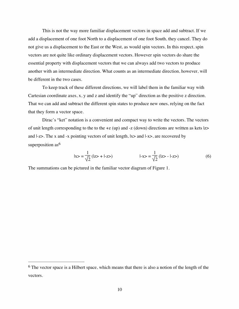
Dirac’s “ket” notation is a convenient and compact way to write the vectors. The vectors

of unit length corresponding to the to the +z (up) and -z (down) directions are written as kets |z>

and |-z>. The x and -x pointing vectors of unit length, |x> and |-x>, are recovered by

superposition as6

|x> = 12 (|z> + |-z>) |-x> =

12 (|z> - |-z>) (6)

The summations can be pictured in the familiar vector diagram of Figure 1.

6 The vector space is a Hilbert space, which means that there is also a notion of the length of the

vectors.

11

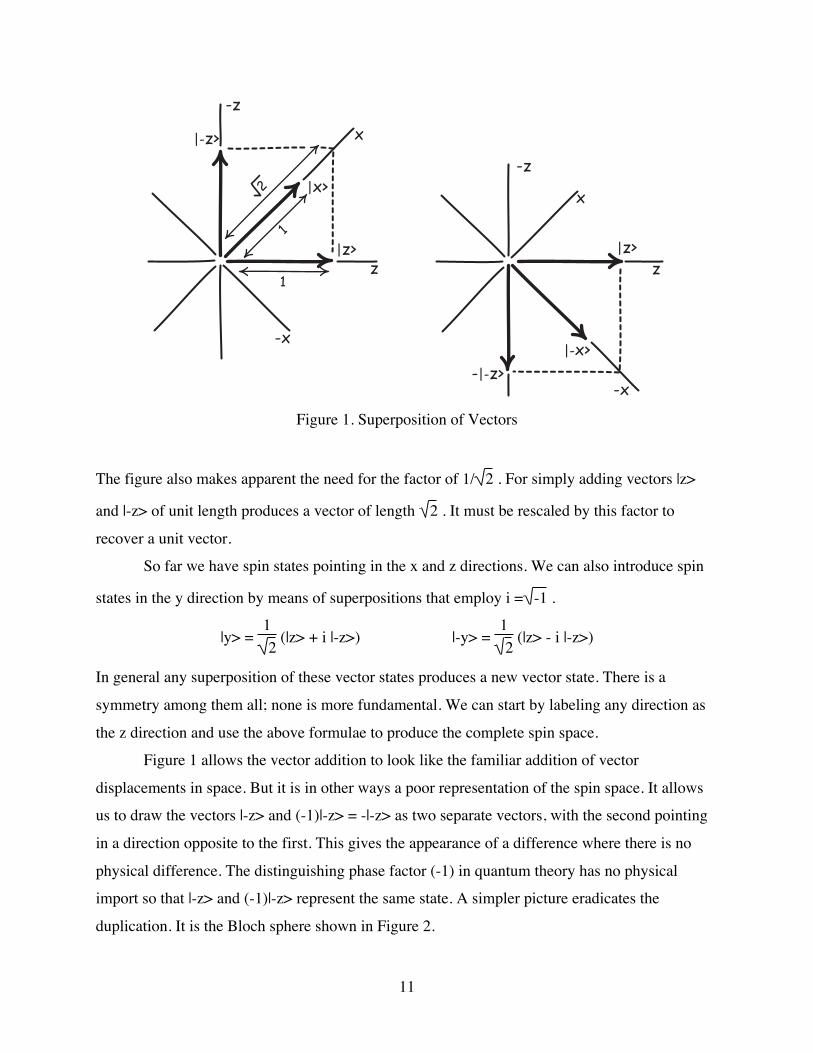
Figure 1. Superposition of Vectors

The figure also makes apparent the need for the factor of 1/ 2 . For simply adding vectors |z>

and |-z> of unit length produces a vector of length 2 . It must be rescaled by this factor to

recover a unit vector.

So far we have spin states pointing in the x and z directions. We can also introduce spin

states in the y direction by means of superpositions that employ i = -1 .

|y> = 12 (|z> + i |-z>) |-y> =

12 (|z> - i |-z>)

In general any superposition of these vector states produces a new vector state. There is a

symmetry among them all; none is more fundamental. We can start by labeling any direction as

the z direction and use the above formulae to produce the complete spin space.

Figure 1 allows the vector addition to look like the familiar addition of vector

displacements in space. But it is in other ways a poor representation of the spin space. It allows

us to draw the vectors |-z> and (-1)|-z> = -|-z> as two separate vectors, with the second pointing

in a direction opposite to the first. This gives the appearance of a difference where there is no

physical difference. The distinguishing phase factor (-1) in quantum theory has no physical

import so that |-z> and (-1)|-z> represent the same state. A simpler picture eradicates the

duplication. It is the Bloch sphere shown in Figure 2.

-z

x

-x

|-z>

|x>

|-x>

|z> |z>z

1

1

2-z

x

-x-|-z>

z

12

Figure 2. The Bloch Sphere

The figure looks so familiar that it is easy to misread. What is orthogonal—“perpendicular”—to

what differs from Euclidean expectations. In this space, |z> and |-z> are orthogonal; as are |x>

and |-x>; and |y> and |-y>. Yet |x> and |z> are not orthogonal, even though Euclidean

expectations suggest otherwise. The sphere also looks like it is a three dimensional vector space

that must be built from three independent basis vectors. However it is a two dimensional space,

with |z> and |-z> as its basis vectors. Their linear superpositions can span the whole sphere since

complex numbers can be used in forming linear superpositions; and this shift from real to

complex numbers gives the added degree of freedom needed.

6.Measurement

6.1AnOddityinQuantumTheory

In non-quantum systems, measuring the state of a system is merely a technical challenge,

not a foundational problem. If we have a spinning top, we can in principle determine the

direction of its axis of spin without having to destroy the top. Things are different in quantum

theory.

We can learn something of the direction of the spin axis of an electron by passing it

through an inhomogeneous magnetic field in a Stern-Gerlach apparatus. The magnetic dipole

moment of the electron aligns with its spin and that moment determines how the electron is

|z>|-z>

|-x>

|x>

|y>

|-y>

13

deflected by the magnetic field. The direction of the deflection tells us the direction of the spin.

We need not delay with further details of this measuring operation save one:

To perform the measurement, we must choose in advance some direction in space along

which to align the magnetic field of the Stern-Gerlach apparatus. Our measurement will be

performed along that direction. The curious and foundationally troublesome property of

measurement in the quantum context is that the measurement will always return a definite result

along the direction chosen, no matter what the spin state of electron.

If we measure the z-spin of an electron that has z-spin up, that is, its state is |z>, we will

measure z-spin up with certainty. If we measure the z-spin of an electron with z-spin down, that

is, its state is |-z> we will measure z-spin down with certainty. So far, there is nothing

unexpected. But if we measure the z-spin of an electron in state |x> with x spin up, something

odd happens. Since a state of x-spin up is different from either z-spin up or z-spin down, you

might expect the measurement to fail in some way. It might, perhaps, give a muddled answer of

both z-spin up and z-spin down and the same time; or perhaps no result at all. That does not

happen. We still get a definite z-spin measurement outcome. It will be either z-spin up or z-spin

down, without any confounding. Which of the two will happen? The formalism gives us a

probability of 0.5 for each.

6.2TheBornRule

In general, a z-spin measurement always returns either a z-spin up or z-spin down

outcome. The probability of each will vary according to the state measured. Standard quantum

theory provides a simple rule—the “Born rule”—for computing these probabilities. Assume that

we are measuring the z-spin of an electron with some general state |φ>. We can decompose the

state vector |φ> into two components in the |z> and |-z> directions.

14

Figure 3. Components of |φ>

The two components are Pz|φ> and P-z|φ>, where the projection operator Pz picks out the

component of |φ> in the |z> direction; and the projection operator P-z picks out the component of

|φ> in the |-z> direction. The vector |φ> is the sum of these two components:

|φ> = Pz|φ> + P-z|φ> (7)

The Born rule tells us that the probability of measuring each outcome is given by the (length)2 of

each of these two component vectors, where we recall that by supposition |φ> has unit length.

Probability (z-spin up) = (length Pz|φ>)2 (8)

Probability (z-spin up) = (length Pz|φ>)2

For the general case of a |ψ> measurement on a state |φ>, we have

Probability (|ψ> on ψ-measurement of |φ>) = (length Pψ|φ>)2 (9)

For the case of |ψ> = |z> and |φ>=|x>, we have from (6) that

|x> = 12 (|z> + |-z>)

so that

Pz|x> =12 |z> P-z|x> =

12 |-z>

as shown in Figure 4. The probability of each outcome is just (length)2 = ⎝⎜⎛

⎠⎟⎞1

2 2

= 0.5.

zz

|φ>

P |φ>

-zP |φ>

-z

15

Figure 4. Projections of |x>

6.3TheBasisoftheDifferenceBetweenProbabilisticandQuantumInductiveLogics

That the Born rule gives us the correct probabilities for measurement outcomes is well

established by experiment. How it can do it and what is happening during the measurement

process, however, remains a troublesome issue in the foundations of quantum theory.

In the standard, text-book account, the electron state vector of the electron undergoing

measurement “collapses” onto one of the two measurement states |z> or |-z>, with the

probabilities given by the Born rule. That is, measurement instantly transforms a |x> state into a

different one, a |z> state or a |-z> state, according to the outcome. Measurement changes the

state. That measurement can do this is odd and puzzling. Yet it is an essential part of the standard

account of quantum theory. An expansive literature has sought to find alternative accounts of

measurement that avoid this oddity. None has produced a view that has been accepted widely

enough to be the new standard.

Fortunately, my present purposes require no decision on how the measurement problem

should be solved. I need adopt only the bare account in which the Born rule gives us the correct

probabilities for measurement outcomes.

This oddity of quantum theory is decisive as far as inductive logics are concerned. For the

probabilities introduced by measurement do not merely reflection an uncertainty over which

prior, existing state is at hand. Measurement changes the state and then attaches probabilities to

the result. As a result, the probabilities of outcomes associated with different measurement

scenarios cannot be combined into a single probability measure. Rather, a different quantity

synthesizes these measures and that quantity forms the basis of a quantum inductive logic.

-zx

|x>-zP |x>

zP |x>z

1

1/ 2

1/ 2

16

7.DensityOperators The goal here is to find the inductive logic warranted by the quantum facts concerning

electrons in entangled states. To proceed, we need to identify the structure in the quantum case

that is analogous to the probability measure of probabilistic logic. That inductive structure is the

density operator. It arises as follows.

For a single particle, in the most definite case, we assuredly have just one quantum state,

such as |z>. It is called a “pure state.” What if we are uncertain as to which of two such pure

states, |z> and |-z>, is at hand? It would be nice if our uncertainty could be captured merely by

taking a suitably weighted sum of the two pure state vectors. That simple option fails. We

already saw that adding these two vectors just gives us another pure state vector. If we add them

with equal weight, for example, we merely recover |x>, as (6) shows.

While this simple option fails, something very close to it succeeds. An alternative way of

representing a pure state is by a projection operator. There is a one to one correspondence

between them, so picking one amounts to picking the other. We have already seen projection

operators in the context of the Born rule of measurement above in equation (8). They pick out the

component of a vector parallel to the direction of projection. For each unit vector, such as |z>,

there will be just one projection operator that finds all of |z> to be in the direction in which it

projects. We have written that unique projection operator as Pz. More compactly, the pure state

|z> is associated uniquely with the projection operator Pz that has the property that Pz |z> = |z>.

Since these projection operators are a special case of density operators, let us explore

them a little more. Operators in vector spaces are the analogs of functions in ordinary algebra. A

function maps numbers to numbers. The square function maps 2 to 4, 3 to 9, and so on. An

operator in the vector space maps vectors to vectors. The projection operator is one of the

simplest. The behavior of the projection operator Pz associated with the vector |z> is fully

specified by the fact that it takes |z> back to itself and takes the vector |-z> to zero:

Pz |z> = |z> Pz |-z> = 0 (10)

and that it is linear, so that

Pz (A |z> + B) |-z>) = A Pz |z> + Pz |-z>)

17

for all complex numbers A and B. Since an arbitrary vector |ψ> can always be written as this

sort of linear sum |ψ> = (A |z> + B) |-z>), linearity and (10) fix how the projection operator acts

on any vector.

Now we return to the original problem. What if we are unsure as to which of |z> and |-z>

is at hand? As long as we represent the states directly by vectors, we cannot just add the two

vectors in a suitably weighted summation. We saw that would give us a new vector, which is just

a different pure state. If we represent states with projection operators, then we can add them

without this happening. If we weight the two states equally, then we produce the new operator

for a so-called “mixed state,” in contrast to the pure states with which we started:

ρmax = 12 Pz + 12 P-z (11)

The subscript “max” indicates that the state is maximally mixed—that is, as far away as

possible—from a pure state. (We will see how this comes about below.) This new operator is no

longer a projection operator.7 It is a density operator. We do not need to use the 12 to 12

weighting. We merely need to use two positive real weights that sum to unity. The 12 to 12

weighting, however, is the case that will interest us most. We arrive at the most general density

operator for the single electron spin by choosing arbitrary positive, real number weights wz and

w-z,

ρ = wz Pz + w-z P-z (12)

such that the weights sum to unity, wz + w-z = 1.

At this stage, it looks as if the density operators of (11) and (12) are behaving just like

probability measures. We appear to be uncertain over which of |z> or |-z> we have with

probabilities wz and w-z, respectively. That appearance is reinforced by the term “mixed state.”

Something like this is correct. But it is not quite like this. The unqualified term “mixed state” is 7 The quickest way to see that is to note that projection operators have the property of

“idempotency.” That is, after they have been applied once, nothing changes if they are applied a

second or third time. That is, Pz Pz = Pz and P-z P-z = P-z. The operator ρmax is not idempotent,

since ρmax ρmax = 14 Pz Pz + 14 P-z P-z + 14 Pz P-z + 14 P-z Pz = 14 Pz + 14 P-z = 12 ρmax ≠ ρmax. (Note

Pz P-z = P-z Pz = 0.)

18

misleading and it is in the qualifications needed that the novelty of the quantum logic will be

found.

8.TensorProductSpaces A density operator is the appropriate structure for an inductive logic when we are

inferring inductively over the properties of electrons in entangled states. These states arise as

follows. Consider two electrons. Each has its own spin vector space. The first is formed by

taking all linear superpositions of the states |z>1 and |-z>1 of the first electron. The second is

formed by taking all linear superpositions of the states |z>2 and |-z>2 of the second particle. (The

subscripts 1 and 2 just number the particles.) The two electrons together form a combined

physical system with its own vector space. One state in it will be a product state such as |z>1|z>2.

That is, the first electron state is z-spin up and the second is z-spin up also. All four of these

possibilities are

|z>1|z>2 , |z>1|-z>2, |-z>1|z>2, |-z>1|-z>2

We form a new vector space, the combined space of all possible states of the two particles, by

taking all linear superpositions of these four states. The space is formed in the same way as we

formed the one electron vector space by taking all linear superpositions of |z> and |-z>. This new

space is the tensor product of the vector spaces associated with the individual particles.

This new vector space contains many new states. We will investigate one, the so called

“singlet state” of total spin angular momentum of zero. It is 8

|s> = 12 (|z>1|-z>2 - |-z>1|z>2) (13)

It is a superposition of two states: |z>1|-z>2 in which the first particle spin points “up” and the

second “down”; and |-z>1|z>2 in which the first particle spin points “down” and the second “up.”

8 The factor of 1/ 2 ensures that the state |s> has unit length. Since the spins in each term point

in opposite directions, the total angular momentum of the singlet state is zero.

19

9.ReducedDensityOperators Consider two entangled electrons, such as the singlet state (13). The two electrons can

remain entangled in the singlet state, even when they are widely separated spatially. If we have

access to just one of these electrons, we can make a measurement of the spin direction of that

one electron. The entanglement means that whatever measurement outcomes we obtain on our

nearby electron will be correlated with the measurement outcomes that someone else finds on the

other remote electron. We read that correlation directly from the two terms in the singlet formula

(13). The first term |z>1|-z>2 tells us that whenever the first electron produces z-spin up on

measurement, the second electron produces z-spin down (and conversely). The second term

|-z>1|z>2 tell us that whenever the first electron produces z-spin down on measurement, the

second produces z-spin up (and conversely). In short, our measurement on the nearby electron

will always give a spin of the opposite direction from the result of a measurement on the remote

electron.

When we make our measurements on the nearby electron, we will know nothing of these

remote outcomes. Let us set them aside and ask what outcomes we should expect for

measurements on the one electron to which we have access. Quantum theory provides the

following recipe for determining the probabilities of the various outcomes.

The first step is to eliminate explicit appearance of the second, remote electron from the

description of the two electron system to arrive at a reduced description of the first, nearby

electron only. We begin by replacing the vector representation of the entangled state by its

corresponding projection operator, P12. For example, the projection operator associated with the

pure singlet state |s> can be written as a sum that includes projection operators associated with

the individual particles that comprise it:

P12 = Ps = 12 Pz,1 P-z,2 + 12 P-z,1 Pz,2 + further cross terms (14)

where the “,1” and “,2” notation labels the nearby and remote electrons (respectively) to which

the individual projection operators belong. The “further cross terms” contain operators that are

20

not projection operators. While important in some applications, these further terms drop out of

the calculations below.9

We now suppress the details of the second remote particle “2” by means of a “trace”

operation “Tr.” This linear operator replaces the degrees of freedom in its scope by their

expectation values. The trace operator Tr2 of the remote electron vector space suppresses the

properties of the remote electron. If P12 is the projection operator associated with the entangled

pair of electrons, we arrive an operator that represents the properties of the first electron only by

means of

ρ1 = Tr2[P12] (15)

The operator ρ1 need no longer be a projection operator, but will in general be a density operator.

Since they are produced in the reducing of the two electron vector space to a one electron space,

they are called reduced density operators. For the case of the singlet state when P12 = Ps, we

have 10

ρs1 = Tr2[Ps] = 12 Pz,1 + 12 P-z,1 = ρmax,1 (16)

The operator ρs1 is not a projection operator.

That the reduced density operator for the nearby electron is not a projection operator

captures the fact that the electron is in no definite spin state. If the entangled pair is in a singlet

state, then the reduced density operator of the nearby electron (16) is the maximally mixed state

(11). One might expect that the two factors of 12 are just the probabilities of measuring z-spin up

and measuring z-spin down. They are.

9 For completeness, the “further cross terms” are -1

2 |z>1<-z|1|-z>2<z|2 - 12 |-z>1<z|1|z>2<-z|2 where

the linear operator |z>1<-z|1 maps |-z>1 to |z>1 and |z>1 to 0; and so on for the remaining three

operators. 10 Since Tr2 [Pz,2] = Tr2 [P-z,2] = 1 and the trace operator is linear, we have

Tr2 [Ps] = Tr2 [ 12 Pz,1 P-z,2 + 12 P-z,1 Pz,2 + further cross terms]

= 12 Pz,1Tr2 [P-z,2] + 12 P-z,1Tr2 [Pz,2] = 12 Pz,1 + 12 P-z,1, where Tr2 [further cross terms] = 0.

21

This follows from the Born rule (9) for measurement outcomes for density operators. In

its general form, the rule says that the probability of measuring a spin state |ψ> when we have an

electron described by a density operator ρ is11

Probability (|ψ> on ψ-measurement of ρ) = Tr[Pψ ρ] (17)

The projection operator Pψ is just the projection operator associated with the vector |ψ>.

Applying this formula to the maximally mixed state ρmaxwe find:12

Probability (z-spin up on z-spin measurement of ρmax) = Tr[Pz ρmax] = 12

Probability (z-spin down on z-spin measurement of ρmax) = Tr[P-z ρmax] = 12 (18)

10.DensityOperatorsdonotRepresentProbabilisticIgnoranceofa

Unique,TrueState

10.1ManyProbabilityMeasures

The density operator ρmax for the maximally mixed state looks initially as if it just

represents a familiar probabilistic uncertainty over whether the true state is |z> or |-z>. The two

coefficents of 12 for the states |z> and |-z> in the expression (11) reappear as the probabilities of

measuring these states according to the Born rule (18).

What makes this mixed state different from mere probabilistic uncertainty is an important

fact about the density operators of mixed states: they can be written in many ways, each

11 While it is written differently, this version of the Born rule is equivalent to (9). Briefly, to go

from (17) to (9), set ρ as the projection operator Pφ associated with the pure state |φ>, then

Tr[Pψ Pφ] = (length Pψ|φ>)2. To go in the reverse direction, set the pure state |φ> in (9) to be a

many electron entangled state and Pψ the projection operator associated with the |ψ> state of one

of the entangled electrons.

12 We have Tr[P|z> ρmax] = Tr[Pz ( 12 Pz + 12 P-z)] = Tr[12 Pz Pz + 12 Pz P-z] = Tr[1

2 Pz] = 12 Tr[Pz] =

12 , where we have used that Tr[Pz] = 1, Pz Pz = Pz, Pz P-z = 0 and the linearity of Tr.

22

indicating a different sort of uncertainty with a distinct probability measure associated with it.

That makes the term “mixed state” potentially quite misleading. The state is not a simple mixture

that can be decomposed uniquely into its components. It is not like a mixture of sand and iron

filings that can be unmixed uniquely with a magnet.

Since this is the key point for all that follows, let us be clear on how this comes about.

The density operator is simply a map that takes vectors to vectors. Two density operators are the

same if they map the same vectors to the same vectors. In this respect, they are no different from

ordinary functions. Take f(x) =x2. It is a function that maps numbers to their squares. While their

expressions look different when written down, the functions g(x) = (x+1)(x-1) +1 and h(x) =

(x+2)(x-2) + 4 perform exactly the same mappings. So they are the same function.

It turns out that the mapping of the maximally mixed state ρmax of (11) can represented

equally well by many equivalent expressions

ρmax = 12 Px + 12 P-x = 12 Py + 12 P-y = 12 Pψ + 12 P-ψ = 12 I (19)

Here Px is the projection operator associated with |x>, Py with |y>, etc. and Pψ is the projection

operator associated with some arbitrarily chosen unit vector |ψ> in the Bloch sphere, pointing in

any direction. I is the identity map that takes each vector back to itself.

Each of the expressions for ρmax in (19) represent the same map on the vector space,

which is written most simply as the last expression on the list, 12 I. That is, ρmax is the map that

merely takes each vector in the space back to a half-sized version of itself. To see that they are

equivalent, we need only recall from (7) that an arbitrary vector |φ> is the sum of its two

components, when decomposed in the + ψ and – ψ directions:

|φ> = Pψ |φ> + P-ψ |φ> = (Pψ + P-ψ ) |φ>

It follows that (Pψ + P-ψ ) is just the identity operator I—that is the operator that merely maps a

vector back to itself. Thus 12 (Pψ + P-ψ ) = 12 Pψ + 12 P-ψ = 12 I. This is true no matter which unit

vector |ψ> is used to define it. Thus the maximally mixed state density operator ρmax is defined

equally well by any of the formulae in (19).

These equivalent representations of the maximally mixed state ρmax provide further

probabilities for measurement outcomes analogous to (18):

23

Probability(x-spin up on x-spin measurement of ρmax) = 1/2 (20)

Probability(x-spin down on x-spin measurement of ρmax) = 1/2

Probability(y-spin up on y-spin measurement of ρmax) = 1/2

Probability(y-spin down on y-spin measurement of ρmax) = 1/2

Probability(ψ -spin up on ψ -spin measurement of ρmax) = 1/2

etc.

10.2NoSingleProbabilityMeasureUnifiesThem

The combined measurement outcomes of (18) and (20) are incompatible with the

ordinary notion of probabilistic uncertainty as mere ignorance of some definite but unknown

state. That sort of ignorance can be captured by a single probability measure, whereas there can

be no single probability measure covering all the results of (20). For each of the states returned

by measurement are incompatible with all the others. An x-spin up state is different from either a

y-spin up and a z-spin up state. An effort to treat these probabilities as generated by ignorance

over some true but unknown state fails and does so rapidly.

Take the probabilities of (18). If we interpret them as this sort of ignorance, then we have

with probability one that the true state of the system is |z> or |-z>. For the two states are mutually

exclusive so that

P(state is truly |z> or |-z>) = P(state is truly |z>) + P(state is truly |-z>) = 1/2 + 1/2 = 1

It now follows that the probabilities of all the other states must be zero, which contradicts the

probabilities reported in (20).

Might we solve the problem with a simple expedient? Take a large outcome space whose

primitive events are of the form:

We measure x-spin and recover x-spin up.

We measure x-spin and recover x-spin down.

We measure y-spin and recover y-spin up.

We measure y-spin and recover y-spin down.

etc.

We can form a single probability measure over this larger outcome space, such that the

probabilities of (20) can be recovered as conditional probabilities. For example:

24

Probability(x-spin up on x-spin measurement)

= Probability (we measure x-spin and recover x-spin up | we measure x-spin)

The difficulty with this proposal is that our space now includes probabilities over our freely

chosen actions, such as:13

Probability (we measure x-spin)

The probabilities of (20) are provided directly by quantum theory itself. These new probabilities

over our actions bring nothing but trouble. What grounds these new probabilities? To secure a

grounding in physical chances, we might employ some physical randomizer to instruct us in

which measurement to make. Then our inductive logic has been restricted to this special case. Or

if we wish to leave the setting as open as possible, then that very openness means that there are

no specific facts that warrant the introduction of the probabilities. In the worst case, they are

arbitrarily chosen subjective probabilities and we corrupt the objectivity of our inductive logic by

mingling them with the objective probabilities of (20). Setting aside this extreme case, we have

still compromised the quantum inductive logic by interweaving inductive support from two

distinct arenas: the inductive support for various quantum measurement outcomes as guided by

quantum theory; and the inductive support for certain of our choices as guided the vagaries of the

human circumstances surrounding our choices.

These are serious difficulties and best avoided. Inductive support for quantum outcomes

ought to be independent of human affairs. There is no need for us to face these difficulties. For

nothing compels us to combine the probability measures of (20) into a single huge measure. We

can arrive at an inductive logic that does not need them, as long as we are willing to give up the

idea that an inductive logic must be probabilistic.

10.3DensityOperatorsastheFundamentalInductiveStructures

The maximally mixed state ρmax already represents some sort of uncertainty over the

electron state. It is not the same as the probabilistic uncertainty familiar from cases of ignorance

arising through random sampling, for such uncertainty cannot issue in the measurement

probabilities (20). The direct way to understand the sort of uncertainty represented by ρmax is

13 Since Probability (we measure x-spin) = Probability(x-spin up on x-spin measurement) +

Probability(x-spin down on x-spin measurement).

25

that it is the inductive structure that does manifest as the infinite list of the measurement

probabilities (20). It is a compact representation of them all.

For many, the predisposition to favor probabilities is strong. They might be inclined to

say that means that the logic is still probabilistic--here finally we have probabilities. However

these probabilities are not the central quantities. They are intermediates that mediate between the

density operator and the measurement outcomes. To capture the inductive situation fully, we

need the entire infinite set. It is insufficient merely to report a subset associated with fewer than

all directions of measurement. One cannot use the rules of the probability calculus to infer from

the measurement probabilities for x-spin measurements, for example, to those for y-spin

measurements.

The density operator is the natural and compact representation of the capacity of the

electron to deliver different measurement results. When we form the new inductive logic adapted

to this quantum case, the density operator is the central quantity that replaces the probability

measure of the more familiar probabilistic inductive logics. It is the quantity that figures

centrally in the physics of entangled electrons, in the same way as physical chances figure

centrally in the physics of roulette wheels. It is the quantity around which we should build an

inductive logic for entangled electrons, just as we build an inductive logic for roulette wheel

outcomes around physical chances.

Note for experts in quantum foundations: My goal here is not to contribute to the

literature in the foundations of quantum theory. Rather it is to find a context in which a non-

probabilistic inductive logic is warranted. Such a context arises, I argue here, with the bare

version of quantum theory that merely employs the Born rule to determine measurement

outcomes but does not probe what happens in the measurement process. If we deviate from this

bare formulation, matters may change. If, for example, we adopt a Bohmian approach, then we

augment our ontology to include hidden electron position properties, possessed always by

electrons and revealed on measurement. Our uncertainties may then revert to the sort of

probabilistic uncertainties that arise with random sampling. Exploring that possibility is not my

project here.

26

11.IstheDensityOperatorReallyanInductiveStructure? Is it really admissible to treat density operators as inductive structures that can serve in an

inductive logic? They seem to be a poor choice for it is hard to say precisely what sort of

uncertainty they represent. They do not represent the familiar sort of uncertainty captured by

probabilities. Why should we erect an inductive logic for quantum theory around density

operators when, perhaps with some effort, we might find a way to replace them with probability

measures?

The short answer is that we should use these density operators since they are the

appropriate structures delivered by the applicable physics. The uncertainty they represent is more

opaque to us than that represented by a probability measure merely because the latter are familiar

and their problems largely tamed. We should not mistake the resulting transparency of

probability measures for their necessity in inductive logics. Indeed the sorts of analyses that

make probability measures interpretationally transparent can be applied equally successfully to

density operators.

To see this, note that probability measures initially require considerable interpretive work

before their meaning becomes clear or clear enough. If we are unprepared, we encounter severe

difficulties when we try to give an explicit definition of probability talk. The challenge is to

complete the formula:

“An outcome has

probability 0.65.”

means [some text here that does not

already contain “probability”].

The difficulty is that “probability” always seems to creep into the text requested. We cannot

complete the formula by saying that the frequency of success in repeated trials approaches 0.65

in the limit of arbitrarily many trials. We must say that this limit is approached with probability

one.

While these are serious difficulties, they do not mean that probability talk is meaningless.

Indeed, we can constrain the meaning of probability talk quite effectively with a few familiar

devices that amount to partial, implicit definitions.14 First, we require that a probability measure

14 I set aside other approaches that interpret probabilities operationally in terms of the behavior

supposedly manifested by people who harbor those probabilities as belief states. For example, to

believe that the probability of an outcome is 1/2 is to be equally ready to accept either side of an

27

conforms to the standard axioms of probability theory. Second we give interpretations of

certainty to the probabilistic extremes: probability one is certainty of occurring; probability zero

is certainty of not occurring. We can use these components to provide interpretations for cases of

intermediate probability. The trick is to embed the probability talk into a larger discourse in

which the already interpreted cases of unit or zero probability arise.

For example, take the proposition that an outcome has probability 0.65. It is a theorem of

the probability calculus that, with probability one, on repeated independent trials, the outcome

will arise with a frequency that approaches 65%. Most people find that gives them enough to

grasp the difference between the two propositions:

An outcome has probability 0.65.

An outcome has probability 0.05.

Loosely speaking, the first outcome happens 13 times as often in repeated trials.

If this sort of interpretive apparatus is sufficient to dispel the clouds around probability

talk, then the clouds surrounding the density operator as an inductive structure can also be

dispelled. For a quite analogous interpretive apparatus can be employed for them.

First, density operators obey a quite definite axiom set and thereby accrue meaning

implicitly, just as do probabilities.15 Second we can identify extreme cases. The most definite is

the density operator corresponding to a pure state such as |z>, a projection operator such as Pz.

This projection operator expresses certainty that we do have the state |z>; and certainty that we

do not have the state |-z>. It is analogous to an outcome of probability one if |z> is the true state

at hand. The maximally mixed density operator of ρmax is the least definite. It favors all spin

directions equally, for under it every possible spin direction has the same probability upon

equal stakes bet on the outcome. In so far as these operational definitions are constitutive of the

probability of an inductive logic, they must be resisted. They entangle probabilities with human

utilities and that is a mortal threat to the objectivity of the bearing of evidence in a probabilistic

logic. For our preference for $100 over $10 ought to have no bearing on whether observation of

the 3K cosmic background radiation increases the probability of the big bang. 15 The details do not matter but are stated here: A density operator is linear operator in the vector

space that is positive and of unit trace.

28

measurement. It is the analog of a uniform probability measure that assigns the same probability

to all simple outcomes.

These most and least definite density operators are the extreme cases. For all the

intermediate cases, we will be able to give a list analogous to (20) of the probabilities of all

possible measurement results. That list gives us the same sort of interpretive purchase on the

associated density operator as does saying something like “probability 0.65 means that the

outcome happens roughly 65% of the time.” Analogously we can say that having some particular

density operator entails that we have such and such probabilities of outcomes on this or that

measurement, where the list includes all possible measurement and outcomes. That is, we know

probabilistically what it is to have some density operator as an inductive structure in terms or all

possible measurement experiences in the world. If we are confident in our understanding of

probabilities as inductive structures, then we should be confident in our understanding of these

density operators as inductive structures.

12.AGeometricPictureofanElectronSpinDensityOperator Part of our comfort with probability measures is that there are simple physical or

geometric models for them. For example, distributing probabilities over different outcomes is

akin to dividing a unit mass into parts and locating different parts on the different outcomes. The

weight of evidence appears directly in the analogy as a mass. Additivity of the probability

measure is captured by the fact that we can only increase the mass on one outcome by reducing

the mass on others by exactly the same amount.16 If we have a probability density over some

continuous space of outcomes, we can picture the space as an area and the probability density at

each point as the altitude of some mountainous surface spread over it.

A fertile picture of all possible probability distributions over n+1 mutually exclusive

outcomes is provided by an n-simplex. For three mutually exclusive outcomes, A, B and C, the

n-simplex is a triangle, as shown in Figure 5. The three vertices represent A, B and C and each 16 This makes it natural for us to think that increasing belief or inductive support in one outcome

must come from diminishing it for other outcomes. There is no necessity for this compensation.

It is or it should be a reflection of the fact that out system happens to be one for which additive

measures are warranted as the appropriate inductive structures.

29

point in the triangle represents a distinct probability measure. The probabilities of each of A, B

or C increase with the proximity of the point to the corresponding vertices. The figure shows

contours of constant probability for P(A), P(B) and P(C).

Figure 5. Probability measures for mutually exclusive outcomes A, B and C.

The interior point shown in the figure represents a probability measure for which P(A) = 0.5 and

P(B) = P(C) = 0.25. For this measure, P(A) is greater than P(B) or P(C) since the representative

point is closer to the A vertex than to the B or C vertex.

In general, there are no correspondingly simple geometric pictures for density operators.

The exception is the special case of the spin space of an electron. All possible density operators

can be represented elegantly in a three dimensional sphere, as shown in figure 6.17 Each density

operator is represented by a single point in or on the sphere.

17 This beautiful picture is elaborated in Penrose (2004), §29.4 and Fig. 29.3.

A

B C

P(A)=1

P(A)=0.5

P(A)=0

P(C)=1

P(C)=0.5

P(C)=0

P(B)=1

P(B)=0.5

P(B)=0

30

Figure 6. Pure and Mixed States

The pure states, corresponding to projection operators, occupy the surface of the sphere. (This

surface by itself is the Bloch sphere we saw in Figure 2 above.) These surface points correspond

to the most definite cases of a single pure state. The points inside the sphere represent density

operators that are not also projection operators. They represent mixed states. The ones closest to

the surface are least mixed and closest in their properties to pure states. The deeper one proceeds

inside the sphere the more mixed the states become. The central point is the maximally mixed

state ρmax.

The sphere representation also affords a simple picture of which pure states are mixed to

yield each density operator. The maximally mixed density operator ρmax lies at the center of the

sphere. Any diameter through the center connects two opposite points on the surface of the

sphere, as shown in Figure 7. The points connected are two pure states that form ρmax.

|z>|-z>

|-x>

|x>

|y>

|-y>purestates

mixedstates

31

Figure 7. The Maximally Mixed State

We read directly from the figure that ρmax can be formed by equal mixtures of pure states |x>

and |-x>; or |y> and |-y>; and so on, as summarized in (19). The multiplicity of possible

decompositions of the mixture is represented by the multiplicity of possible diameters through

the center.

There is a corresponding representation for the remaining density operators. Consider

another density operator ρ that is not the maximally mixed ρmax. Any chord through it will

intersect the surface of the sphere at two points, as shown in Figure 8.

|z>

|x>

|y>

|-y>

|-z>

|-x>

ρmax

1/2

1/2

32

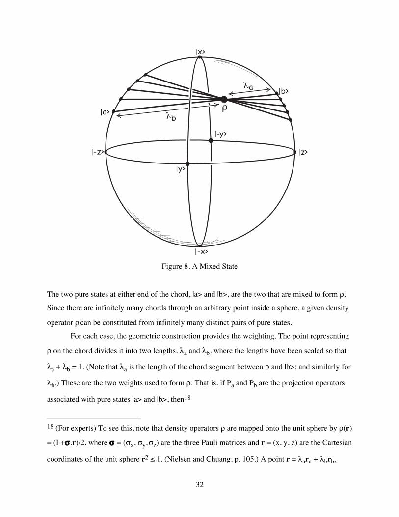
Figure 8. A Mixed State

The two pure states at either end of the chord, |a> and |b>, are the two that are mixed to form ρ.

Since there are infinitely many chords through an arbitrary point inside a sphere, a given density

operator ρ can be constituted from infinitely many distinct pairs of pure states.

For each case, the geometric construction provides the weighting. The point representing

ρ on the chord divides it into two lengths, λa and λb, where the lengths have been scaled so that

λa + λb = 1. (Note that λa is the length of the chord segment between ρ and |b>; and similarly for

λb.) These are the two weights used to form ρ. That is, if Pa and Pb are the projection operators

associated with pure states |a> and |b>, then18

18 (For experts) To see this, note that density operators ρ are mapped onto the unit sphere by ρ(r)

= (I +σ .r)/2, where σ = (σx, σy, σz) are the three Pauli matrices and r = (x, y, z) are the Cartesian

coordinates of the unit sphere r2 ≤ 1. (Nielsen and Chuang, p. 105.) A point r = λara + λbrb,

|z>

|x>

|a>

|b>a

|y>

|-y>

|-z>

|-x>

ρbλ

λ

33

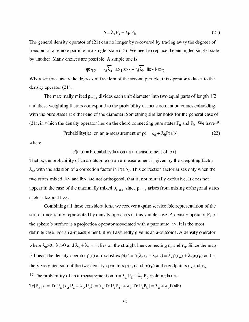
ρ = λaPa + λb Pb (21)

The general density operator of (21) can no longer by recovered by tracing away the degrees of

freedom of a remote particle in a singlet state (13). We need to replace the entangled singlet state

by another. Many choices are possible. A simple one is:

|ψ>12 = λa |a>1|z>2 + λb |b>1|-z>2

When we trace away the degrees of freedom of the second particle, this operator reduces to the

density operator (21).

The maximally mixed ρmax divides each unit diameter into two equal parts of length 1/2

and these weighting factors correspond to the probability of measurement outcomes coinciding

with the pure states at either end of the diameter. Something similar holds for the general case of

(21), in which the density operator lies on the chord connecting pure states Pa and Pb. We have19

Probability(|a> on an a-measurement of ρ) = λa + λbP(a|b) (22)

where

P(a|b) = Probability(|a> on an a-measurement of |b>)

That is, the probability of an a-outcome on an a-measurement is given by the weighting factor

λa, with the addition of a correction factor in P(a|b). This correction factor arises only when the

two states mixed, |a> and |b>, are not orthogonal, that is, not mutually exclusive. It does not

appear in the case of the maximally mixed ρmax, since ρmax arises from mixing orthogonal states

such as |z> and |-z>.

Combining all these considerations, we recover a quite serviceable representation of the

sort of uncertainty represented by density operators in this simple case. A density operator Pa on

the sphere’s surface is a projection operator associated with a pure state |a>. It is the most

definite case. For an a-measurement, it will assuredly give us an a-outcome. A density operator where λa>0, λb>0 and λa + λb = 1, lies on the straight line connecting ra and rb. Since the map

is linear, the density operator ρ(r) at r satisfies ρ(r) = ρ(λara + λbrb) = λaρ(ra) + λbρ(rb) and is

the λ-weighted sum of the two density operators ρ(ra) and ρ(rb) at the endpoints ra and rb.

19 The probability of an a-measurement on ρ = λa Pa + λb Pb yielding |a> is

Tr[Pa ρ] = Tr[Pa (λa Pa + λb Pb)] = λa Tr[PaPa] + λb Tr[PaPb] = λa + λbP(a|b)

34

close to Pa will give an a-outcome on a-measurement with high probability. For it will most

commonly be associated with a value of λa close to one.20 As the location of the density operator

approaches the midpoint, the probability of an a-outcome on a-measurement will approach 0.5,

which is the probability associated with the maximally mixed density operator at the center of

the sphere. This maximally mixed density operator treats all pure states alike: the probability of

an a-outcome on a-measurement is 0.5, no matter what |a> is. That it must do this is immediately

clear from the fact that the sphere has a rotational symmetry about the center of the sphere. From

that central point, no pure state is closer than any other. It must treat all alike.

13.LeiferandSpekkens’SystemofQuantumInference So far, we have seen only a part of the inductive logic appropriate to entangled electrons.

We have identified the reduced density operator in each single electron’s vector space as the

structure corresponding to the probability measure in a probabilistic logic. We need to do only a

little more to specify the full logic. That is, we need a full specification of which density

operators arise in which circumstances. As it happens, no further theorizing is needed to arrive at

this specification. It is given to us by the standard formalism of quantum theory. When the theory

lays out the physics of how the reduced density operators of entangled electrons relate, it is also

giving us the inductive logic.

One may wonder, however, if what results really is an inductive logic. If one is used to

and is expecting a probabilistic logic, it will be unfamiliar, just as density operators are not quite

like probability measures. But that is no reason to dismiss it. Lack of familiarity is not the same

as failure.

Leifer and Spekkens (2013) have shown, however, that the inductive logic based on

density operators is not so unfamiliar after all. Once we adopt the density operator as the basic

inductive structure, they have shown how we can rewrite basic results in quantum theory so that

they are structurally analogous to formulae in a probabilistic logic. Their system is elaborate and

20 If the density operator is close to Pa but λa is not close to one, it is because the density

operator lies on a chord whose other endpoint, Pb, is also close to Pa. Then the correction term

λbP(a|b) will ensure that the probability of an a-outcome on a-measurement remains high.

35

distinguishes connections between variables according to whether they are causally or acausally

related. To give a quite preliminary sense of the system, I will describe how it treats the case of

acausally related systems, such as the two particles in a singlet state.

The following Table 1, based on Leifer and Spekkens (2013, p. 7), summarizes the

correspondences:

Probabilistic logic Quantum inductive logic

Classical variables R, S, … over an outcome

space.

Systems A, B, … supporting (Hilbert) vector

spaces HA, HB,

Probability measures P(R), P(S), … Density operators ρA, ρB, …

Joint probability distribution P(S&R) over

Cartesian product space. Density operator ρAB over the tensor product

Hilbert space HAB = HA⊗ HB

Conditional probability measure P(S|R)

defined through

P(S&R) = P(S|R) P(R)

P(S|R) = P(S&R) / P(R)

Conditional density operator defined through

ρAB = ρB|A ★ ρA

ρB|A = ρAB ★ ρA-1

Normalization

ΣS P(S|R) = 1

Normalization

TrB (ρB|A) = IA

where IA is the identity operator in HA.

Total probability21

P(S) = ΣR P(S&R) = ΣR P(S|R) P(R)

ρB = TrA (ρAB) = TrA (ρB|A ★ ρA)

Table 1. Correspondences between Probabilistic and Quantum Logics

These correspondences are fairly straightforward. In the mutation example, the classical

variables R, S, … are the genetic make-ups of each child. When R, S, etc. take specific values,

then the genetic makeup of the child is specified as a particular mutation, m1, m2, … and their

totality forms the outcome space. In the case of entangled electrons, systems A, B, … correspond

21 This the same rule at (5) above, but here written in the notation used by Leifer and Spekkens.

36

to electron1, electron2, … and the vector spaces HA, HB,… are the vector spaces of electron

states described above.

The remaining formulae have been written in a way that emphasizes the parallels

between the two cases. The classical summation operation “ΣS…” sums away the variable S.

Correspondingly, the trace operator TrB (...) averages away the degrees of freedom associated

with B. The star operation ★ is a particular multiplication operation designed to keep the parallel

in the formulae as close as possible. The goal is to find the quantum analog of P(S&R) = P(S|R)

x P(R), where the “x” is just ordinary arithmetic multiplication, since the probabilities P(.) are

real numbers. One might write ρAB = ρB|A . ρA, as a direct analog of the probabilistic formula.

But caution is needed, since there are important disanalogies. The operation joining ρB|A and ρA

is not simple multiplication, but the sequential application of operators, since ρB|A and ρA are

operators that act on vectors. This produces two problems.

The first is that the two operators act on different vector spaces. ρB|A acts on vectors in

HA⊗ HB . ρA acts on vectors in HA. If they are to be combined, they must act on the same vector

space. The simple remedy is to expand ρA to ρA⊗ IB, where the addition of …⊗ IB makes a new

operator that acts as ρA on HA and as the identity (“do nothing”) on HB.

The second is that the order in which we combine the operators will matter, whereas it

does not matter when we multiply real numbers. The formula ρB|A . ρA says first act with ρA and

then with ρB|A. The formula ρA. ρB|A says first act with ρ B|A and then with ρA. There is no

assurance that the two will yield the same result; and in general they will not. Which is the

correct order? It turns out that neither is correct if the resulting product is to be a new density

operator. To make sure it will be a density operator, we split the operator ρA into a product of its

square root, so that ρA = ρA1/2 . ρA1/2. Instead of multiplying ρB|A by ρA, we multiply it from

either side by ρA1/2. The formula that results from both changes is the definition of the star

operator:

ρAB = (ρA1/2 ⊗ IB) ρB|A (ρA1/2 ⊗ IB) = ρB|A ★ ρA (23)

An inversion gives an explicit expression for ρB|A

37

ρB|A = (ρA-1/2 ⊗ IB) ρAB (ρA-1/2 ⊗ IB) = ρAB ★ ρA-1 (24)

14.AnalogousInferences:MutationsandElectrons In the case of mutations among children, we used the rule of total probability (5) in the

series of computation (2), (3) and (4), to infer from the probabilities of various mutations in one

child in the family to the corresponding probabilities for a second child. We can use these new

quantum formulae to display the corresponding inference for pairs of electrons in the singlet

state.

Take two electrons in the singlet state (13)/ (14) with projection operator P12. Using (16)

and (19), the reduced density operator representing each of the electrons individually is

ρ1 = I1/2 ρ2 = I2/2 (25)

These are the quantum analogs of the probabilistic equation (1) of the mutation case:

P(child1 carries mi) = ri << 1 i=1,…,n

P(child2 carries mi) = ri << 1 i=1,…,n

A short calculation shows that22

ρ1|2 = 2 P12 (26)

The analog of the rule of total probability in Table 1 is

ρ1 = Tr2 (P12) = Tr2 (P1|2 ★ ρ2)

Substituting for P1|2 and ρ2, we use this rule to infer from state ρ2 of the second electron to that

of the first ρ1. We find

ρ1 = Tr2 (P12) = TrA (2P12 ★ I2/2) = I1/2 (27)

in agreement with (25). This last computation (27) is the quantum analog of the application of

the classical rule of total probability in (2), (3) and (4).

22 This follows directly from (24) once we note that ρ11/2 = I1/ 2 so that ρ1-1/2 = 2 I1.

38

15.Disanalogies These last comparisons underscore the analogies between a probabilistic inductive logic

and the quantum inductive logic induced by the laws of quantum theory onto electrons in

entangled states. That these analogies are present shows that the quantum logic is of comparable

richness to the probabilistic logic. The key point for our purposes, however, is that the analogies

are incomplete. The quantum inductive logic is a distinct inductive logic.

That the analogies are incomplete is already established by the investigation of the

properties of density operators in Section 10. When the formal properties of the quantum

inductive logic are explored, further disanalogies emerge. They derive from the fact that

probabilities are numbers, whose products are insensitive to the order of multiplication, whereas

density operators are sensitive to the order of multiplication. Switch that order and one may get a

different result.

One consequence of the lack of commutativity of operators is the following disanalogy

discussed in Leifer and Spekkens (2013, p. 33). The probability P(S&R) can be expanded as a

simple product

P(S&R) = P(S|R) P(R)

The rule is robust and holds if all the probabilities are themselves further conditionalized on

another variable T:

P(S&R|T) = P(S|R&T) P(R&T)

This is extremely useful in probabilistic analysis since it means that we can collect all

background information into some huge proposition T and then treat all probabilities

conditionalized on T, P(.|T), as if they were unconditional probabilities P(.).

The first of these two formulae has a quantum analog

ρAB = ρB|A ★ ρA

However the second does not. That is, we do not in general have

ρAB|C ?=? ρB|AC ★ ρA|C

This means that the rule for forming conditional states will differ according to whether or not we

begin with a state that is itself already conditional.

39

16.Conclusion The material theory of induction requires that the inductive logic applicable in some

domain be dictated by the facts that prevail in that domain. In many domains, facts do warrant a

probabilistic inductive logic. The prevalence of such domains has helped foster the

misimpression that a probabilistic logic is the universal logic of induction.

The burden of this chapter has been to illustrate how a formally rich, alternative inductive

logic can be warranted. The domain is that of entangled quantum mechanical particles. The

inductive logic appropriate to them employs density operators where a probabilistic inductive

logic employs probability measures. This new logic looks very different, initially, from a

probabilistic logic. There is no single real valued measure of support that tells us which state is

more or less well supported. Differences of support are expressed by density operators. In the

most definite case of narrowest support, the density operator is a projection operator. It identifies

a unique state as the true state. At the opposite extreme of the most distributed support, the

maximally mixed density operator accords equal support to all states, just as does a uniform

probability measure in the probabilistic case. The intermediate cases are captured by density

operators between these extremes. For the case of a single electron, the range of cases and their

properties are represented in readily interpretable form by the spheres of Section 12.

There are further structural analogies between the quantum inductive logic and a

probabilistic logic, as described in Leifer and Spekkens (2013). That assures us that we do have a

logic of comparable richness. Eventually, the analogies break down, for the two logics are

different.

ReferencesM. S. Leifer and Robert W. Spekkens (2013), “Towards a formulation of quantum theory as a

causally neutral theory of Bayesian inference,” Physical Review A 88, 052130 (2013);

preprint: “Formulating Quantum Theory as a Causally Neutral Theory of Bayesian

Inference,” arXiv:1107.5849 [quant-ph]

Nielsen, Michael A. and Chuang, Isaac L. (2010) Quantum Computation and Quantum

Information. Cambridge: Cambridge University Press.

Penrose, Roger (2004) The Road to Reality. London: Jonathan Cape.