Embed Size (px)
Citation preview
A QR Decomposition Approach to Factor Modeling of
Multivariate Time Series
A THESIS
submitted by
IMMANUEL DAVID RAJAN M
for the award of the degree
of
MASTER OF SCIENCE
(by Research)
Department of Electrical Engineering
arX
iv:1
811.
1130
2v1
[st
at.C
O]
27
Nov
201
8

Indian Institute of Technology Madras, India.
April 2014
i

Dedicated to mom and dad for their care,
and grandparents for their love.
ii

THESIS CERTIFICATE
This is to certify that the thesis entitled A QR Decomposition Approach to Factor Modeling of
Multivariate Time Series, submitted by Immanuel David Rajan M, to the Indian Institute of
Technology Madras, for the award of the degree of Master of Science (Research), is a bonafide
record of the research work carried out by him under my supervision. The contents of this thesis,
in full or in parts, have not been submitted to any other Institute or University for the award of any
degree or diploma.
Dr. Bharath Bhikkaji
Professor and Research Guide,
Dept. of Electrical Engineering,
IIT Madras, Chennai - 600036.
Place: Chennai
Date: 11-4-2014

ACKNOWLEDGEMENTS
The fun and elegance of research was motivated primarily by my guide and mentor Dr. Bharath
Bhikkaji. His free approach towards research enabled me to develop the curiosity needed to explore
various fields which made the prospect of doing research both fun and entertaining. He also helped
me along the path of research and pointed me in the right directions when I needed it. It’s of note
to mention that he never once did say that he ain’t got the time. All in all, the best Guide to have.
I thank Dr. Girish Ganesan, Santa Fe partners LLC, for his valuable comments and criticisms.
He also gave the finance data to be analysed and helped in interpreting the results.
The two courses that I felt were great are “Speech Signal Processing” by Dr. Umesh Srinivasan
and “Applied Time Series Analysis” by Dr. Arun Thangirala. These two courses were entertaining
and the assignments were fun to solve.
Life here in IITM would have been bland if not for my friends (Instrumentation and Control lab
mates and my Hostel friends). Of particular mention, Mithun for always being there and helping
out in any way (annoyance included); Pankaj (Drama Queen) for he’ll kill me if I don’t mention
him; Pavan, for all those long pointless but interesting talks; Jayesh, for being that awesome crazy
friend.
Last but not the least, I’d like to thank my family for supporting me through this endeavour.
My mom, Vanathi, for her prayers and my Dad, Dr. Manohar Jesudas, for providing inspiration
and motivation. My sister, Grace Nithia for her pestering and all other family members for being
i

a critic.
ii

ABSTRACT
An observed K-dimensional series {yn}Nn=1 is expressed in terms of a lower p-dimensional latent
series called factors fn and random noise εn. The equation, yn = Qfn + εn is taken to relate the
factors with the observation. The goal is to determine the dimension of the factors, p, the factor
loading matrix, Q, and the factors fn. Here, it is assumed that the noise co-variance is positive
definite and allowed to be correlated with the factors. An augmented matrix,
M ,
[Σyy(1) Σyy(2) . . . Σyy(m)
]
is formed using the observed sample autocovariances Σyy(l) = 1N−l
∑N−ln=1 (yn+l − y) (yn − y)>,
y = 1N
∑Nn=1 yn. Estimating p is equated to determining the numerical rank of M . Using Rank Re-
vealing QR (RRQR) decomposition, a model order detection scheme is proposed for determining
the numerical rank and for estimating the loading matrix Q. The rate of convergence of the esti-
mates, as K and N tends to infinity, is derived and compared with that of the existing Eigen Value
Decomposition based approach. Two applications of this algorithm, i) The problem of extracting
signals from their noisy mixtures and ii) modelling of the S&P index are presented.
iii
Contents
ACKNOWLEDGEMENTS i
ABSTRACT iii
1 Introduction 1
1.1 Outline of the Proposed approach . . . . . . . . . . . . . . . . . . . . . . . . 3
1.2 Chapter Outline . . . . . . . . . . . . . . . . . . . . . . . . . . . . . . . . . . 7
1.3 Contributions of this thesis . . . . . . . . . . . . . . . . . . . . . . . . . . . . 9
2 Data Model and Summary of Algorithm 11
2.1 Assumptions on the Data . . . . . . . . . . . . . . . . . . . . . . . . . . . . . 11
2.2 Summary of the Algorithm . . . . . . . . . . . . . . . . . . . . . . . . . . . . 14
3 Existing Algorithms 15
3.1 PCA based Method . . . . . . . . . . . . . . . . . . . . . . . . . . . . . . . . 15
3.2 EVD Method . . . . . . . . . . . . . . . . . . . . . . . . . . . . . . . . . . . 18
4 RRQR Decomposition 21
5 Model order: A Numerical Rank Perspective 38
6 Perturbation Analysis of Q 60
6.1 Perturbation analysis of QR decomposition: . . . . . . . . . . . . . . . . . . . 60
6.2 Convergence Analysis of Q . . . . . . . . . . . . . . . . . . . . . . . . . . . . 63
7 Comparison with the EVD Method 71
8 Illustration and Simulations: 77
8.1 Simulation 1 . . . . . . . . . . . . . . . . . . . . . . . . . . . . . . . . . . . . 77
iv
8.2 Simulation 2 . . . . . . . . . . . . . . . . . . . . . . . . . . . . . . . . . . . . 81
8.3 Simulation 3 (ICA Pre-processing) . . . . . . . . . . . . . . . . . . . . . . . . 83
8.4 Application on a finance portfolio . . . . . . . . . . . . . . . . . . . . . . . . 87
9 Conclusion and Discussions 89
Appendix 1 93
Concepts from Linear Algebra . . . . . . . . . . . . . . . . . . . . . . . . . . . . . 93
Appendix 2 96
landau notations and Mixing Properties . . . . . . . . . . . . . . . . . . . . . . . . 96
Bibliography 103
v

List of Tables
8.1 Summary of the results of Simulation 1,all values multiplied by 1000. . . . . . 79
8.2 Summary of Observations from Simulation 2. The RMSE and FE values are mul-tiplied by 1000. . . . . . . . . . . . . . . . . . . . . . . . . . . . . . . . . . . 83
8.3 Errors Associated when used as pre-processing with ICA . . . . . . . . . . . . 87
8.4 Results from finance data application . . . . . . . . . . . . . . . . . . . . . . . 88
vi

List of Figures
8.1 Convergence of∥∥∥Q−Q∥∥∥
Ffor EVD and RRQR for fixed K = 60 . . . . . . . 79
8.2 Plot of ratio of eigen values of MM>, ri (3.5) , for fixed K = 180; N = 100. . 80
8.3 Plot of ratio of diagonal values ofR inMΠ = QR, ri, (1.13), where Π is got usingRRQR Method for fixed K = 180; N = 100. . . . . . . . . . . . . . . . . . . 80
8.4 ICA implementation Model . . . . . . . . . . . . . . . . . . . . . . . . . . . . 85
vii

Terminology
Matrix Notations
1. Let an ∈ RK and bn ∈ RK , n = 1, 2, ..., N be two vector valued stochastic processes. Thecross-covariance between them is denoted by,
Σab(k) , E {(A[n+ k]− E{A}) (B[n]− E{B})} , (1)
where E{.} is the expectation operator.
2. The sample covariance (finite time approximation) is denoted by,
Σab(k) ,1
N − k
N−k∑n=1
(an+k − a)(bn − b)>, (2)
where a and b are the sample means of the stochastic series {an} and {bn} given by a =1N
∑Nn=1 an, b = 1
N
∑Nn=1 bn respectively.
3. The difference between the sample covariance and the ideal estimate is denoted by the per-turbation
∆Σab(k) , Σab(k)− Σab(k). (3)
Order Notations
The following notations are used for denoting the asymptotic convergence rates:
1. Let {an} and {bn} be deterministic sequences. an = O(bn) implies, there exists a constantM > 0 such that, 0 < limn→∞
anbn≤M.
2. an � bn implies for a given integer n0 > 0 there exists m, M > 0 such that m <| anbn|< M ,
for all n > no.
3. an = o(bn) implies, limn→∞anbn
= 0.
4. A stochastic sequence {an} is said to be of smaller order (o) in probability to the determin-istic sequence {bn}, denoted by an = oP (bn), if an
bn→P 0 where→P denotes convergence
in probability. That, given ε > 0 there exists an δ > 0 and an integer n0 > 0 such thatP (| an
bn|< ε) > 1− δ, ∀n > n0. In other words P (| an
bn|< ε)→ 1 as n→∞.
5. Similarly with {an}, a stochastic sequence, and {bn}, a deterministic sequence, an = OP (bn)implies, given ε > 0 there exists a constantM > 0 such that P (| an
bn|< M) ≥ 1−ε, ∀n ≥ n0
6. an �P bn implies, given ε > 0 there exists constants m, M > 0 such that P (m <| anbn|<
M) ≥ 1− ε, ∀n ≥ n0
viii

For more details on the order notations refer ([24, pp 53-55]) and also Appendix 2.
Miscelanious Notations
1. The MATLAB notations are used to address various blocks of the matrix:(a) A(:, j) refers to the jth column of A
(b) A(j, :) refers to the jth row of A
(c) A(a : b, c : d) refers to the block of A consisting of rows a to b and columns c to d
2. The σi (A) notation is used to indicate the ith highest singular value of the matrixA ∈ Rm×n.
3. λi (A) reperesents the ith largest eigen value of the matrix A.
ix
Chapter 1
Introduction
Factor modeling refers to modeling observations in terms of its constituent factors. In Multivariate
Statistics, factor modeling refers to modeling a given high dimensional series called “observations”
in terms of lower dimensional time series called “factors”. A linear relationship
yn = Hxn + εn, n = 1, 2, . . . , N, (1.1)
is assumed between the observations and the factors. Here yn ∈ RK is the observed data, xn ∈ Rp
the vector of factors, H ∈ RK×p the factor loading matrix and εn ∈ RK×1 being the random noise.
Without loss of generality, it could be assumed that yn and εn are of zero mean.
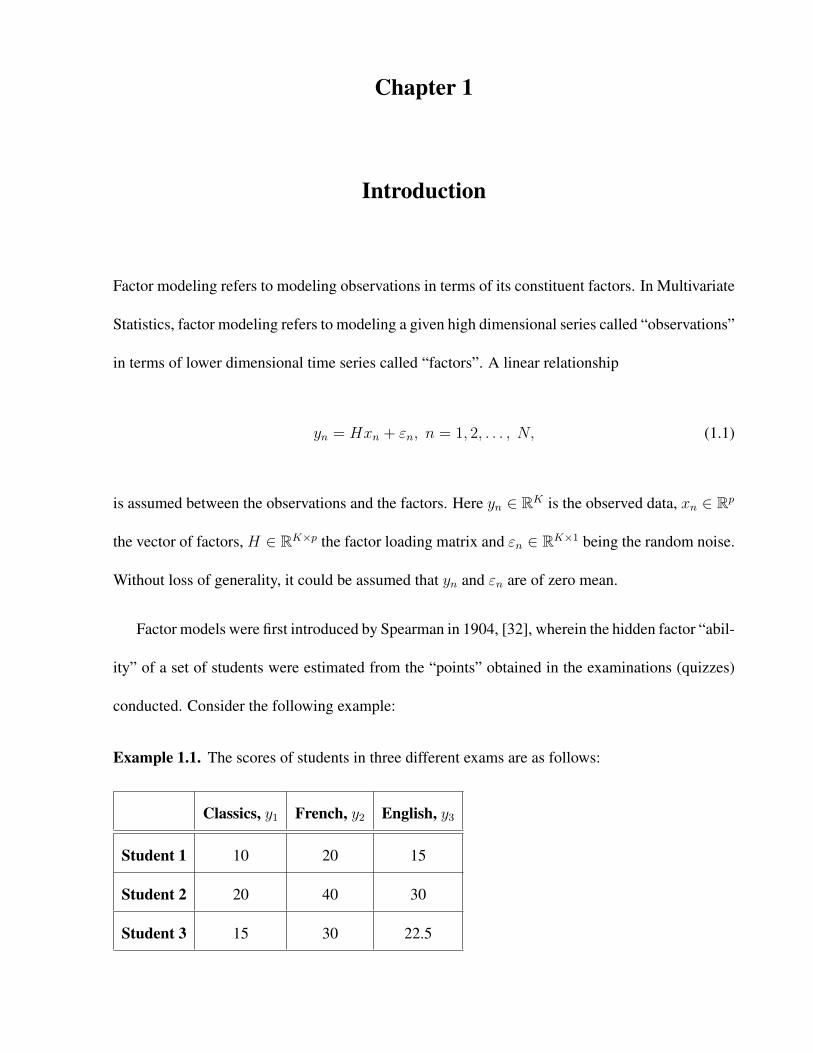
Factor models were first introduced by Spearman in 1904, [32], wherein the hidden factor “abil-
ity” of a set of students were estimated from the “points” obtained in the examinations (quizzes)
conducted. Consider the following example:
Example 1.1. The scores of students in three different exams are as follows:
Classics, y1 French, y2 English, y3
Student 1 10 20 15
Student 2 20 40 30
Student 3 15 30 22.5
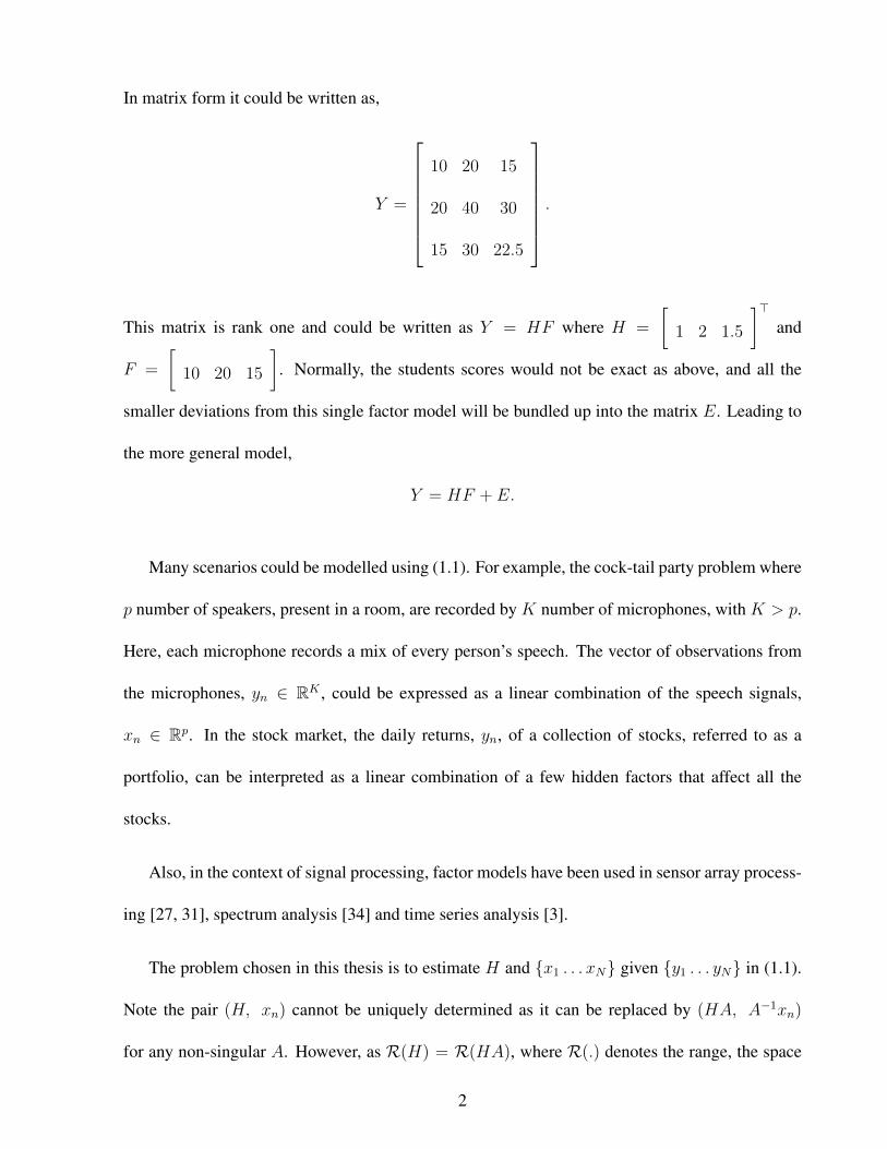
In matrix form it could be written as,
Y =
10 20 15
20 40 30
15 30 22.5
.
This matrix is rank one and could be written as Y = HF where H =
[1 2 1.5
]>and
F =
[10 20 15
]. Normally, the students scores would not be exact as above, and all the
smaller deviations from this single factor model will be bundled up into the matrix E. Leading to
the more general model,
Y = HF + E.
Many scenarios could be modelled using (1.1). For example, the cock-tail party problem where
p number of speakers, present in a room, are recorded by K number of microphones, with K > p.
Here, each microphone records a mix of every person’s speech. The vector of observations from
the microphones, yn ∈ RK , could be expressed as a linear combination of the speech signals,
xn ∈ Rp. In the stock market, the daily returns, yn, of a collection of stocks, referred to as a
portfolio, can be interpreted as a linear combination of a few hidden factors that affect all the
stocks.
Also, in the context of signal processing, factor models have been used in sensor array process-
ing [27, 31], spectrum analysis [34] and time series analysis [3].
The problem chosen in this thesis is to estimate H and {x1 . . . xN} given {y1 . . . yN} in (1.1).
Note the pair (H, xn) cannot be uniquely determined as it can be replaced by (HA, A−1xn)
for any non-singular A. However, as R(H) = R(HA), where R(.) denotes the range, the space
2
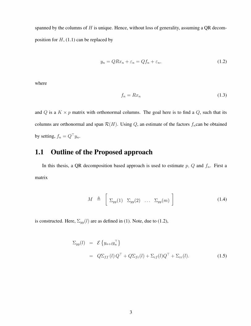
spanned by the columns of H is unique. Hence, without loss of generality, assuming a QR decom-
position for H , (1.1) can be replaced by
yn = QRxn + εn = Qfn + εn, (1.2)
where
fn = Rxn (1.3)
and Q is a K × p matrix with orthonormal columns. The goal here is to find a Q, such that its
columns are orthonormal and span R(H). Using Q, an estimate of the factors fncan be obtained
by setting, fn = Q>yn.
1.1 Outline of the Proposed approach
In this thesis, a QR decomposition based approach is used to estimate p, Q and fn. First a
matrix
M ,
[Σyy(1) Σyy(2) . . . Σyy(m)
](1.4)
is constructed. Here, Σyy(l) are as defined in (1). Note, due to (1.2),
Σyy(l) = E{yn+ly
>n
}= QΣff (l)Q> +QΣfε(l) + Σεf (l)Q
> + Σεε(l). (1.5)
3

Assuming that the factors are not correlated with the future noise, i.e.,Σεf (l) = E{εn+lf
>n
}= 0,
and the noise not having correlations across time, i.e., Σεε(l) = E{εn+lε
>n
}= 0 leads to,
Σyy(l) = Q[Σff (l)Q> + Σfε(l)
].
Thus,
M = Q
[Σff (1)Q> + Σfε(1) . . . Σff (m)Q> + Σfε(m)
], QP, (1.6)
where
P =
[P1 P2 . . . Pm
](1.7)
with
Pl = Σff (l)Q> + Σfε(l). (1.8)
Assuming all factors have a non-zero correlation at least in one of the lags l = 1, . . . ,m, implies
P is full row rank (i.e., P is of rank p). This further implies that M is also of rank p.
Hence the QR decomposition [14, 12],
M , QR, (1.9)
ofM , (1.4), withQ being an orthonormal matrix would have an upper triangularR with lastK−p
4

rows being zeros, i. e.,
R =p
K − p
R11
0
K×mK
.
Thus Q is obtained by setting
Q , Q(:, 1 : p),
the first p columns of Q (in MATLAB Notations) and an estimate of the factors is obtained by
setting fn = Q>yn. Note, for any permutation matrix Π∈ RmK×mK such that the first p columns
of MΠ are linearly independent, would have a QR decomposition of the form
MΠ , QR, (1.10)
with R having the last K − p rows as zeros. A different Q can be obtained by setting Q ,
Q (:, 1 : p). As both Q(:, 1 : p) and Q(:, 1 : p) span the same column space, there need not be any
specific preference of one over the other. However, it would be prudent to choose a Π such that the
p columns selected by Π have the best condition number.
In the finite data case M , (1.4), is replaced by
M ,
[Σyy(1) Σyy(2) . . . Σyy(m)
], (1.11)
where Σyy(l) is as in (2). Note rank(M)6= p, in fact it will be of full rank (rank
(M)
=K) with
probability one. The determination of p and Q from M are not as trivial as before. The matrix M
could be interpreted as a perturbed version of the matrix M ,
M = M + ∆M
5
or in more general form,
MΠ = MΠ + ∆MΠ.
And the problem could be restated as finding an estimate of MΠ from MΠ. A general QR decom-
position,
MΠ ,p mK − p[Mp MmK−p
]
,
[Qp QK−p
] R11 R12
0 R22
= QR, (1.12)
where R22 6= 0. Assuming rank (M) = p, an estimate of MΠ can be obtained by setting,
MΠ = Q(:, 1 : p)R11. For a good approximation of MΠ, it is desirable to have a Π such
that σmin(R11
)� σmax
(R22
), where σmin (.) denotes the minimum singular value and σmax (.)
denotes the maximum singular value. Rank Revealing QR (RRQR) algorithms are a class of algo-
rithms that find a permutation matrix Π such that either,
maxΠ
(σmin
(R11
))
or,
minΠ
(σmax
(R22
))or both are satisfied. Using such a Π, a good estimate of MΠ can be obtained by setting, MΠ =
QpR11. An the estimate of the factor loading matrix and the factors can be got by setting, Q = Qp
6

and fn = Q>yn respectively.
So far, rank (M) = p was assumed to be known. Determination of rank (M) from M , is
obtained by equating it to the determination of numerical rank, [13, 33], of the matrix M . In this
thesis, an RRQR based approach is used to determine numerical rank. An estimate, p, of rank (M),
is set to,
p = arg maxi
γi + ε
γi+1 + ε, (1.13)
where γi and γi+1 are the ith and i + 1th diagonal values of R, (1.12), got by assuming numerical
rank to be i in the Hybrid-III RRQR algorithm [7] with ε = γ1√NK
.
Note, Hybrid-III RRQR algorithm satisfies the bounds in Hybrid-I algorithm and hence could
also be used in estimation of factor loading matrix Q. Here, Hybrid-I algorithm is used because of
its lesser numerical complexity.
In this thesis, asymptotic analysis of the estimates, p, Q and fn are presented. The rates of
convergence of the estimates, when the dimension of the observations K and the duration of the
observations N tends to infinity, under the constraint Kδ√N
= o(1), are derived. It is shown that
the proposed algorithm has better convergence rates than the Eigen Value Decomposition (EVD)
based approach, [22], under certain conditions.
1.2 Chapter Outline
In Chapter 2, the regulatory conditions under which the proposed algorithm is designed are
summarized along with a step-by-step implementation procedure for the proposed algorithm.
In Chapter 3, the two existing algorithms for factor modeling, namely the Principal Component
Analysis Method [20, 2, 3, 19, 26] and the EVD based method, are discussed in detail.
7

In Chapter 4, a detailed exposition of RRQR algorithms are presented along with derivation of
bounds satisfied by the Hybrid algorithms.
In Chapter 5, the problem of finding the number of factors, p from M is discussed in the
numerical rank perspective. The asymptotic rate of convergence for the estimate of the model
order p as K,N →∞ is presented therein.
In Chapter 6, the Convergence of Q obtained by using M to Q obtained from M is studied.
The asymptotic rates are also got for the same.
In Chapter 7, the proposed algorithm is compared with the existing EVD based algorithm of
[22].
In Chapter 8, the numerical results obtained by simulating the algorithm using Monte-Carlo
trials is presented and compared with other existing algorithms. There is also the simulation of the
famous cock-tail party problem wherein the proposed algorithm is used as pre-processing for the
popular Independent Component Analysis (ICA) technique. A real life application of the proposed
algorithm to the finance market is also presented.
Finally, in Chapter 9, concludes with a discussion of the entire thesis along with the prospect
of further developments.
8

1.3 Contributions of this thesis
In this thesis, a new algorithm for factor modeling is proposed. While other popular algorithms
like the PCA based algorithms have quite stringent constraints on noise εn i.e.,
E{fnε>m
}= 0, ∀ n, m (1.14)
and
E{εnε>m} = σ2In×nδ (n−m) , (1.15)
where In×n is an Identity matrix and δ(l) is the Kronecker delta function, the proposed algorithm
has less stringent constraints allowing the factors to be correlated with the past noise and also that
noise can have any-covariance Σ.
The proposed algorithm is subjected to rigorous asymptotic analysis wherein
• Rate of convergence of the model order estimate p, (1.13), to p as K,N →∞ are derived.
• Convergence rates of the factor loading matrix Q and factors fn as K,N → ∞ are also
derived.
From these asymptotic properties, it was found that the proposed algorithm performs better than
the EVD based algorithm proposed in [22] in certain scenarios.
Two interesting applications of the proposed algorithm is also discussed.
• The Cock-tail party problem of separating multiple signals from their linear noisy mixtures.
• Modeling the S&P 500 index and predicting the daily returns of individual companies.
9

This page is intentionally left blank
10

Chapter 2
Data Model and Summary of Algorithm
In this chapter, the Data Model and assumptions upon which the proposed algorithm works are
summarized in Section (2.1). Section (2.2) gives a step-by-step implementation procedure for the
proposed algorithm.
2.1 Assumptions on the Data
Regulatory Conditions
The data model assumed as (1.1). Now, the factors could be written as
X = [x1, x2, . . . , xN ] =[x(1), x(2), . . . , x(p)
]>
where xn ∈ Rp represents the values taken by the factors at the nth instant and x(i) ∈ RN represents
the ith factor which is a series in time n = 1, . . . N . Now, assume that linear combination of all
the factors could result white noise, then, the last factor x(p) could be written as
x(p)n = en +
∑i 6=p
αix(i)n , n = 1, . . . , N

where en is a white noise sequence. Thus, replacing the pair (H, xn) in (1.1) with the pair
(HA−1, Axn) with A =
1
1
. . .
1
−α1 −α2 . . . −αp−1 1
would result in the factors f = Axn =
[x(1), x(2), . . . , e
]>where e is a white noise sequence. Thus, since e is white noise, it does not
have correlation at any lags l = 1, . . . , m. Thus, the rank of M in (1.4) would be (p− 1) and
the last factor would not be detected by the proposed algorithm. Thus, the following condition is
assumed.
(A1) No linear combination of the factors x(i), results in white noise i.e.,[Σxx(1) . . . Σxx(m)
]is of rank p (full row rank).
The following three conditions could be deduced from (1.5):
(A2) The noise ε is not correlated with past factors, i.e., Σεx (k) = cov(εn+k, xn) =
Z, ∀k > 0 where Z is a zero matrix.
(A3) The factors xncan have correlation with past noise εn, i.e., cov(xn+k, εn) need not
necessarily be Z but bounded as N,K →∞.
(A4) The auto-covariance of the noise needs to be bounded, i.e., cov(εn, εn) is bounded as
N,K →∞.
The following mixing conditions, [10, pp 67-77], ensures that as N →∞, M , (1.11), tends to M ,
(1.4) for a fixed K, i.e., the finite sample estimates converge to the ensemble average.
12

(A5) The process {yn} is a zero mean strictly stationary process with ψ mixing with mixing
coefficients ψ{.} satisfying∑
n≥1 nψ(n)12 < ∞ also E(|yn|4) < ∞ element wise.
refer ([10]) for a comprehensive study of mixing properties. The ψ mixing could also
be replaced with α mixing with mixing coefficient αn = O (n−5) and E(|yn|12) <∞
element wise. For properties regarding the same, refer Theorem 27.4 in ([6]). Refer
the Appendix 2 for more details regarding mixing properties.
Factor Strength
A factor is considered a strong factor if it affects all the observed outputs and a weak factor if
not. To model this mathematically, the columns ofH determine the strength with which the factors,
xn, affect the observations, yn. The following two assumptions on the columns of H quantify the
impact of the factors on the observations:
(A6) The columns of the matrix H =
[h1 h2 . . . hp
]are such that, O
(‖hi‖2
2
)=
O(K1−δ), i = 1, 2, ..., p and 0 ≤ δ < 1.
(A7) The columns of H are independent of each other, i.e.,
O
minθj
∥∥∥∥∥hi −∑j 6=i
θjhj
∥∥∥∥∥2
2
= O(K1−δ) (2.1)
The above assumptions A1-A7 are quite similar to the ones made in ([22]).
Finally, consider the following notations used to denote the strength of factor correlation with
noise:
13

Definition 2.1. Define
κmax , max1≤l≤m
‖Σfε(l)‖2 (2.2)
κmin , min1≤l≤m
σmin (Σfε(l)) (2.3)
where κmax and κmin correspond to a measure of factor correlation with noise.
2.2 Summary of the Algorithm
In this section, the steps in implementation of the proposed algorithm are presented.
1. Let {yn}Nn=1 be the observed data. And the data model is assumed as in (1.2).
2. Compute M defined in (1.11), where Σyy(l) is got by (3.4).
3. To evaluate the Numerical Rank, p,(a) Set i = 1
(b) First the permutation matrix Π is got by using HYBRID-III algorithm assuming a nu-merical rank of i.
(c) Take Gram-Schmidt QR (GS-QR) decomposition of MΠ i.e., MΠ = QR. Computeri = γi+ε
γi+1+εwhere γi and γi+1 are the ith and i+1th diagonal values of R and ε = γ1√
KN.
(d) Set i = i+ 1
(e) Repeat Until i < P where, P is taken such that p < P .
4. Now, estimate of numerical rank, p, is got by finding the i that maximizes ri as in (1.13).
5. Evaluate RRQR decomposition of M using HYBRID-I algorithm ([7]) presented in Algo-rithm (4.2). Let the RRQR Decomposition be as in (1.12).
6. Now, the finite sample estimate of Q is got by, QN,K = Q(:, 1 : p).
7. Finally the estimate of factors is got by, fn = Q>N,Kyn.
An exposition of RRQR-Algorithms are presented in Chapter (4).
14
Chapter 3
Existing Algorithms
In this chapter, two existing algorithms for factor modeling are analysed. Section 3.1 discusses
the PCA based method of factor analysis and Section 3.2 covers the Eigen Value Decomposition
based method.
3.1 PCA based Method
The PCA based method is dealt in many literature, notably [20, 2, 3, 19, 26]. Assume that the
observed time series{yn ∈ RK
}Nn=1
could be modelled as,
yn = Qfn + εn
where, fn ∈ Rp are factors and εn ∈ RK is random noise. The factors and noise are assumed to
satisfy:
Condition_1: The factors and noise are uncorrelated with each other i.e., Σfε(l) = E{fn+lε
>l
}=
0, ∀l.
Condition_2: The noise should have covariance given by Σεε(l) = E{εn+lε
>l
}= δ(l)σ2I, where
δ(l) is the Kronecker delta function and I ∈ RK×K is an Identity matrix.
Under the above conditions, the autocovariance matrix of the observations is
Σyy(0) = E{yny
>n
}= QΣff (0)Q> + σ2I.
Assuming that Σff (0) to be full rank, implies that QΣff (0)Q> is of rank p and will have p non-
zero positive Eigen Values. Let λ1 ≥ λ2 ≥ . . . ≥ λp be the eigen values of QΣff (0)Q>. The
Eigen Value Decomposition of Σyy(0) is,
Σyy(0) = U
λ1 + σ2
. . .
λp + σ2
σ2
. . .
σ2
U>
Thus, the number of factors equal p and the factor loading matrix could be set to, Q = U(:, 1 : p),
the eigen vectors that correspond to the largest p Eigen values. The factors are then fn = Q>yn.
Henceforth, this technique will be refered to as PCA.
Now, the above procedure is ideal. In practice, Σyy(0) will be replaced by its sample co-
variance, Σyy(0) = 1N
∑Nn=1 yny
>n . In which case, estimating the number of factors and the factor
loading matrix becomes a bit more difficult. The problem of finding the number of factors is dealt
as a model order selection problem using AIC (Akiake Information Criteria) and MDL (Minimum
Code Length, [29]) in [26]. In [4], an alternative Information Theoretic Criteria is proposed and
proved to be better than the AIC, [1], BIC (Bayesian Information Criteria) and all of their derivat-
ives. In [4], the model order is taken as the p that minimizes the Information Content,
ICp = ln(V (p, fn)
)+ p
(K +N
KN
)ln
(KN
K +N
)
16

where
V (p, fn) = minQ
1
KN
N∑n=1
∥∥∥yn − Q(p)f (p)n
∥∥∥2
2
Here, Q(p) and f (p)n are obtained using PCA by assuming model order as p. Thus, the estimate of
model order is
pN,K = arg minp{ICp}.
For more details regarding the same, refer [4].
To estimate the factor loading matrix, a Maximum Likelihood framework is used. The Max-
imum Likelihood framework for factor analysis was first introduced by Lawley in the year 1940,
[23]. A detailed version of this ML approach is given in, [19, 28, 4, 20].
Let,
Σyy(0) = U ΛU>
be the eigen value decomposition of Σyy(0), where Λ is a diagonal matrix of eigen values arranged
in descending order, λ1 ≥ λ2 ≥ . . . ≥ λK . It was proved in [28], that the optimal solution to the
ML estimate for the error co-variance, σ2I , is given by σ2 =∑K
i=p+1 λi and the ML estimate for
Q is given by Q = U (:, 1 : p).
The disadvantages of this PCA based method are,
1. The ML estimate inherently assumes yn is iid Gaussian (Though in real life simulations, itcould not be ensured).
2. The requirement of conditions 1 and 2 regarding the noise εn and factors fn as stated before.
3. No properties of the factors fn are taken into consideration.
17

3.2 EVD Method
Recently, Lam et. al., had proposed a new technique for factor modeling, [22]. This technique
helps in overcoming the disadvantages pointed out in the previous PCA based method.
In [22], the authors setup a matrix
S ,m∑l=1
Σyy(l)Σyy(l)> (3.1)
= MM>,
where M is as defined in (1.4). From (3.1) and (1.6),
S = QPP>Q>. (3.2)
As S is an K ×K positive semi-definite matrix with rank p (assuming the p× p matrix PP>
to be full rank), its Eigen value decomposition
S = UΛU> (3.3)
would have a diagonal matrix Λ with the first p diagonal elements strictly positive and the rest
K − p diagonal elements being zero. The factor loading matrix was chosen to be Q = U(:, 1 : p),
the first p columns of U corresponding to the non-zero Eigen values. Here, U(:, 1 : p) refers to
the MATLAB notation of selecting first p columns. An estimate fn of the factors was obtained by
setting fn = Q>yn.
In practice, the auto-covariances Σyy(k), Σff (k) and Σfε(k) k = 0, 1, 2, . . . are approximated
18

by their corresponding finite sample equivalents, for example Σyy(k) is replaced by
Σyy(k) =1
N − k
N−k∑n=1
(yn+k − y) (yn − y)> , (3.4)
where y , 1N
∑Nt=1 yn. The Eigen values of the matrix S formed using (3.4) will not have K − p
zero Eigen values. In fact all the Eigen values will be different with probability 1. Therefore, p
cannot be directly determined by computing the Eigen values of S. In [22], the model order, p,
was estimated using
p = arg max1<i<R
λiλi+1
(3.5)
where λi > λi+1 denotes the Eigen values of the matrix S arranged in descending order. The
properties of this ratio based estimator (3.5) are summarized in [21].
The Proposed QR decomposition based algorithm will be compared with this algorithm in
Chapter 7 with regards to asymptotic properties of their estimates and in Chapter 8 through their
simulations.
19

This page is intentionally left blank
20

Chapter 4
RRQR Decomposition
In this chapter, the RRQR algorithms used in this thesis are discussed in detail. The derivations of
the results pertaining to the RRQR algorithm are presented in this chapter for the sake of comple-
tion.
Define a matrix A of dimension m× n such that,
A ,
[a1 a2 . . . an
],
where ai is an m dimensional column vector. The QR decomposition of A is given by:
A = QR, (4.1)
[a1 a2 . . . an
]=
[q1 q2 . . . qn
]
< a1, q1 > < a2, q1 > . . . < an, q1 >
0 < a2,q2 > . . . < an, q2 >
0 0. . . ...
0 0 0 < an, qn >
where q′is are the orthonormal columns of Q, R is the upper triangular matrix and < , > denotes
inner product. There are many algorithms to achieve the above decomposition refer [12, 14] for
more details.

In the above equation, the matrix Q and R could be segmented as
Q =p m− p[Q1 Q2
]
R ,
p n− p
p
m− p
R11 R12
0 R22
, (4.2)
for any p < min (n,m). From (4.1), it can be seen that the minimum singular value of R11,
σmin (R11) is dependent on the columns a1, . . . , ap of A and maximum singular value of R22,
σmax (R22), depends on the columns ap+1, . . . , an of A. Thus permuting the columns of A and
taking QR would result in different σmin (R11) and σmax (R22). Let Π be a permutation matrix, the
QR decomposition of AΠ be given by,
AΠ = QR.
Given a p < min (m,n), RRQR algorithms are a group of algorithms that find a Π such that,
Π , arg maxΠ∈P
σmin
(R11
)(4.3)
or
Π , arg minΠ∈P
σmax
(R22
)(4.4)
or both, where P is a set of all permutation matrices and R11, R22 are got by segmenting R as in
(4.2). The algorithms that solve (4.3), (4.4) or both (4.3) and (4.4) are are termed, Type I, Type II
22

and Type-III algorithms respectively, [7].
In this thesis, the Hybrid RRQR algorithms proposed by Chandrasekaran et. al., [7], are of
particular interest. The Hybrid-I algorithm is a type I algorithm that satisfies,
σmin (R11) ≥ σp (A)√p(n− p+ 1)
,
σmax (R22) ≤ σmin (R11)√p(n− p+ 1).
The Hybrid-II is a type -II algorithm that satisfies
σmax (R22) ≤ σp+1 (A)√
(p+ 1)(n− p)
σmin (R11) ≥ σmax (R22)√(p+ 1)(n− p)
.
Finally, the Hybrid-III algorithm combines the best of the previous two bounds to ensure,
σmax (R22) ≤ σp+1 (A)√
(p+ 1)(n− p)
σmin (R11) ≥ σp (A)√p(n− p+ 1)
.
Derivation of these bounds can be found in [7]. These derivations are also presented later in this
chapter for the sake of completion.
To understand the working of the Hybrid algorithms, one needs to understand the working of
two other algorithms: the QR decomposition with Column Pivoting (QR-CP) algorithm proposed
by Golub, [14], which is a Type-I algorithm and its corresponding Type-II version proposed by
Stewart (Stewart-II) in [33].
23

The following theorem relates to Interlacing Property of singular values. It is essential for
understanding the rest of the thesis:
Theorem 4.1. Let Σ ∈ Rm×n, m < n, and Σk×l11 , k < l, be any sub matrix of Σ with σ1 ≥ σ2 ≥
. . . ≥ σm and λ1 ≥ λ2 ≥ . . . ≥ λk being their corresponding singular values. Then,
σj ≥ λj ≥ σn−k+j, j = 1, 2...k.
Proof. Refer to Appendix 1.
QR-CP Algorithm
Let the matrix to be permuted be A ∈ Rm×n. The algorithm is as follows:
Initialize s = 0; Π = I ∈ Rn×n.
Let
j = arg maxi ‖A(:, i)‖2 .
if j 6= 1, interchange 1st and jth column of Π and take QR decomposition1,
AΠ = Q(0)R(0),
1Householder or Gram Schmidt methods.
24

where R(s) denotes the matrix R being segmented as,
R(s) ,
s n− s
s
m− s
R(s)11 R
(s)12
0 R(s)22
.
Repeat s = s+ 1;
j = arg maxi
∥∥∥R(s)22 (:, i)
∥∥∥2
if j 6= 1,
Interchange columns s+ 1 and s+ j of Π and retriangularize R(s)Π = QR(s+1)2.
Until s < min (n, m).
Note that R(s)11 and R(s)
22 changes in dimension with every increase in s
The above QR-CP algorithm is an approximation of the greedy algorithm which selects columns
such that σmin(R
(s)11
)is maximized. For further details regarding this approximation, refer [7, pp
596-598].
Now, to look at the properties of the QR-CP algorithm, let
AΠ = QR
where Π is obtained using QR-CP algorithm. The following two lemmas summarize the properties
of QR-CP algorithm:
2Let AΠ = QR. If RΠ = QR, Then, AΠΠ = QQR. Thus, finding permutations to columns of R is equivalent tofinding permutations to columns of A.
25
Lemma 4.1. The diagonal elements in R satisfy
γi ≥σi (A)√n− i+ 1
, i = 1, . . . ,min (n, m) . (4.5)
where γi is the ith diagonal element of R.
Proof. From (4.1) and the above algorithm, it can be seen that γi corresponds to the highest 2 −
norm among the columns of R(i−1)22 . Since R(i−1)
22 has n− i+ 1 columns,
γi ≥
∥∥∥R(i−1)22
∥∥∥F√
n− i+ 1.
Since∥∥∥R(i−1)
22
∥∥∥F≥∥∥∥R(i−1)
22
∥∥∥2,
γi ≥
∥∥∥R(i−1)22
∥∥∥2√
n− i+ 1. (4.6)
Interlacing property3 of Singular Values [14, 25] states that:
σs
(R)≥∥∥∥R(s)
22
∥∥∥2≥ σs+1(R). (4.7)
Thus, combining (4.6) and (4.7) leads to (4.5).
Lemma 4.2. When using QR-CP and segmenting R as in (4.2),
σmin (R11) ≥ σp (A)√pn2p
. (4.8)
Proof. Note R11 could be written as
R11 = DW.
3Refer Appendix 1 on page 93 for a more elegant proof on Interlacing property.
26

where D = diag (R11) is a diagonal matrix with diagonal elements of R11. By the property of
QR-CP algorithm, the diagonal elements of R11 are the highest elements. Thus, W is an upper
triangular matrix such that the diagonal elements are equal to 1 and the rest of the elements are
less than 1. Thus,
σmin (R11) ≥ σmin (D)σmin (W )
Since, for a diagonal matrix, the singular values equal the diagonal elements, from (4.5),
σmin (D) ≥ σp (A)√n− p+ 1
.
Thus, since σmin (W ) = 1‖W−1‖2
,
σmin (R11) ≥ σp (A)√n− p+ 1 ‖W−1‖2
.
Now, ‖W−1‖2 ≤√p2p refer [7, pp 606], thus, we get (4.8).
The above proof is paterned after the proof provided in [7] for the same.
An implementation scheme for the QR-CP algorithm when applied to M , (1.11), is summarized
in Algorithm 4.1.
Stewart’s Type-II Algorithm
The Stewart’s Type-II algorithm proposed first in [33] is discussed here. In, [7], this Stewart’s
algorithm is framed as a type-II equivalent of the QR-CP algorithm. In, [7], both Type-I and
Type-II algorithms were unified in a single framework. This unification enables derivation of
the properties of the Type-II algorithm from its Type-I equivalents. Note Stewart-II algorithm is
27
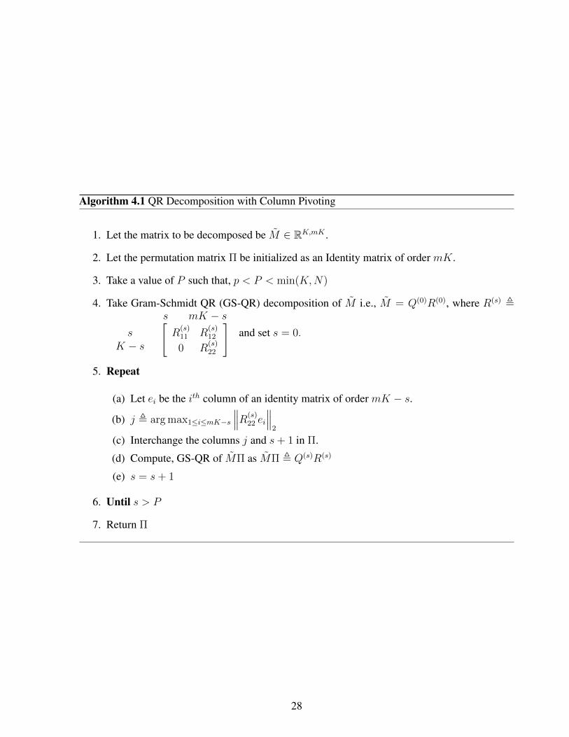
Algorithm 4.1 QR Decomposition with Column Pivoting
1. Let the matrix to be decomposed be M ∈ RK,mK .
2. Let the permutation matrix Π be initialized as an Identity matrix of order mK.
3. Take a value of P such that, p < P < min(K,N)
4. Take Gram-Schmidt QR (GS-QR) decomposition of M i.e., M = Q(0)R(0), where R(s) ,s mK − s
sK − s
[R
(s)11 R
(s)12
0 R(s)22
]and set s = 0.
5. Repeat
(a) Let ei be the ith column of an identity matrix of order mK − s.
(b) j , arg max1≤i≤mK−s
∥∥∥R(s)22 ei
∥∥∥2
(c) Interchange the columns j and s+ 1 in Π.
(d) Compute, GS-QR of MΠ as MΠ , Q(s)R(s)
(e) s = s+ 1
6. Until s > P
7. Return Π
28

applicable only for Invertible matrices.
Unification
Assume A ∈ Rn×n is invertible and of numerical rank p. For details regarding Numerical rank
refer Chapter 5. For now, just take p as the block size used for segmenting R in (4.1).
Note, the Type-II formulation is equivalent to,
minΠσmax (R22) = min
Π
1
σmin(R−1
22
)=
1
maxΠ
(σmin
(R−1
22
)) . (4.9)
Let,
RΠ , QR, R ,
R11 R12
0 R22
Assuming R to be invertible, inverting both sides of the above equation leads to,
Π>R−1 =
R−111 −R−1
11 R12R−122
0 R−122
Q>.
Now, taking transpose on both sides,
R−>Π = Q
R−>11 0
−R−>22 R>12R
−>11 R−>22
. (4.10)
Thus from (4.10), (4.9) and the fact that σmin(R−1
22
)= σmin
(R−>22
); It can be seen that applying
Type-II algorithm to R is equivalent to Type-I algorithm applied to R−>. To make it more clearer,
29

applying Type-I algorithm to R−> gives,
R−>Π = QP,
where
P =
n− p p
n− p
p
P11 P12
0 P22
. (4.11)
Note in Type-I algorithm σmin (P11) is maximized. With some block permutations the above P
could be written as,
p n− p
p
n− p
P22 0
P12 P11
Now, permuting the rows and columns of the individual blocks,
P =
p n− p
p
n− p
JpP22Jp 0
Jn−pP12Jp Jn−pP11Jn−p
where Jl are permutation matrices of order l with ones along the anti-diagonal. This ensures P is
lower triangular. Now, the above P is equivalent to the structure in (4.10), thus Jn−pP11Jn−p can be
equated to R−>22 and from (4.9), maximizing σmin(R−>22
)is equivalent to minimizing σmax (R22)
which is the original Type -II problem. Thus, from the above it is evident that applying a Type-
I algorithm to the rows of the inverse of a matrix A is equivalent to applying Type-II algorithm
directly to A.
30
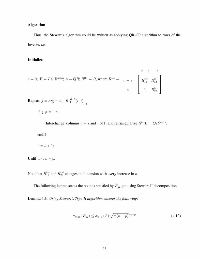
Algorithm
Thus, the Stewart’s algorithm could be written as applying QR-CP algorithm to rows of the
Inverse, i.e.,
Initialize
s = 0; Π = I ∈ Rn×n; A = QR; R(0) = R, where R(s) =
n− s s
n− s
s
R(s)11 R
(s)12
0 R(s)22
.
Repeat j = arg maxi
∥∥∥R(s)−111 (i, :)
∥∥∥2
if j 6= n− s,
Interchange columns n− s and j of Π and retriangularize R(s)Π = QR(s+1).
endif
s = s+ 1;
Until s < n− p.
Note that R(s)11 and R(s)
22 changes in dimension with every increase in s
The following lemma states the bounds satisfied by R22 got using Stewart-II decomposition.
Lemma 4.3. Using Stewart’s Type-II algorithm ensures the following:
σmax (R22) ≤ σp+1 (A)√n (n− p)2n−p (4.12)
31

Proof. Using Type-I, QR-CP algorithm (4.11) ensures (ref (4.8)),
σmin (P11) ≥ σn−p (A)√n− pn2n−p
. (4.13)
Using Unification principle, P11 = R−>22 also, using (4.9) leads to,
σmax (R22) =1
(σmin (P11)). (4.14)
Thus from (4.13) and (4.14), (4.12) is got.
Given a matrix A ∈ Rn×n. Applying Stewart-II algorithm assuming a numerical rank of n− 1
would ensure that, the column with the lowest 2− norm in A gets permuted with the last column.
Note, the weakest column inA is the column that has the lowest 2-norm or the row with the highest
2-norm in A−1.
Hybrid Algorithms
The Hybrid Algorithms are got by combining QR-CP and the Stewart-II algorithm. The first
Hybrid algorithm we’ll be dealing with is the Hybrid-I algorithm.
Consider the matrix A ∈ Rm×n with numerical rank p. The QR decomposition of A be given
32

by A = QR. Now, segment R in two different ways,
R ,
p n− p
p
m− p
R11 R12
0 R22
, (4.15)
,
p− 1 n− p+ 1
p− 1
m− p+ 1
R11 R12
0 R22
. (4.16)
The Hybrid-I algorithm works by iterating between the QR-CP algorithm applied to R22 and
Stewart-II algorithm applied to R11, until no permutations occur. The Stewart-II applied to R11
ensures that the pth column in R is the weakest column (the column with the lowest 2-norm) in
R11. Also QR-CP applied to R22, ensures that the pth column of R is the best column (column
with the highest 2-norm) in R22 (4.16).
Hybrid-I satisfies both the QR-CP and Stewart-II’s conditions. Note, QR-CP to R22 to get the
pth column of R ensures that,
rpp ≥∥∥R22
∥∥2√
n− p+ 1, (4.17)
where rpp is the pth diagonal element of R (refer to (4.6)). Since R22 (4.15) is a sub matrix to R22,
rpp ≥‖R22‖2√n− p+ 1
. (4.18)
Also, Stewart-II applied to R11 (4.15) ensures that
rpp ≤ σmin (R11)√p. (4.19)
33
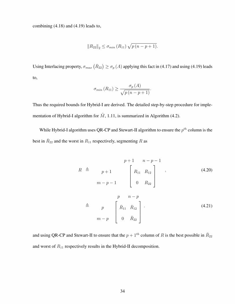
combining (4.18) and (4.19) leads to,
‖R22‖2 ≤ σmin (R11)√p (n− p+ 1).
Using Interlacing property, σmax(R22
)≥ σp (A) applying this fact in (4.17) and using (4.19) leads
to,
σmin (R11) ≥ σp (A)√p (n− p+ 1)
.
Thus the required bounds for Hybrid-I are derived. The detailed step-by-step procedure for imple-
mentation of Hybrid-I algorithm for M , 1.11, is summarized in Algorithm (4.2).
While Hybrid-I algorithm uses QR-CP and Stewart-II algorithm to ensure the pth column is the
best in R22 and the worst in R11 respectively, segmenting R as
R ,
p+ 1 n− p− 1
p+ 1
m− p− 1
R11 R12
0 R22
, (4.20)
,
p n− p
p
m− p
R11 R12
0 R22
. (4.21)
and using QR-CP and Stewart-II to ensure that the p+ 1th column of R is the best possible in R22
and worst of R11 respectively results in the Hybrid-II decomposition.
34
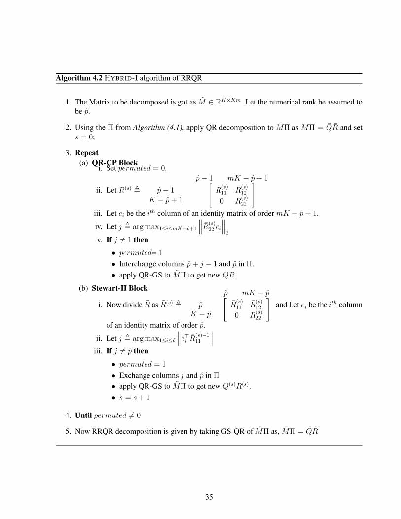
Algorithm 4.2 HYBRID-I algorithm of RRQR
1. The Matrix to be decomposed is got as M ∈ RK×Km. Let the numerical rank be assumed tobe p.
2. Using the Π from Algorithm (4.1), apply QR decomposition to MΠ as MΠ = QR and sets = 0;
3. Repeat(a) QR-CP Block
i. Set permuted = 0.
ii. Let R(s) ,
p− 1 mK − p+ 1
p− 1K − p+ 1
[R
(s)11 R
(s)12
0 R(s)22
]iii. Let ei be the ith column of an identity matrix of order mK − p+ 1.
iv. Let j , arg max1≤i≤mK−p+1
∥∥∥R(s)22 ei
∥∥∥2
v. If j 6= 1 then
• permuted= 1• Interchange columns p+ j − 1 and p in Π.• apply QR-GS to MΠ to get new QR.
(b) Stewart-II Block
i. Now divide R as R(s) ,
p mK − pp
K − p
[R
(s)11 R
(s)12
0 R(s)22
]and Let ei be the ith column
of an identity matrix of order p.
ii. Let j , arg max1≤i≤p
∥∥∥e>i R(s)−111
∥∥∥iii. If j 6= p then
• permuted = 1
• Exchange columns j and p in Π
• apply QR-GS to MΠ to get new Q(s)R(s).• s = s+ 1
4. Until permuted 6= 0
5. Now RRQR decomposition is given by taking GS-QR of MΠ as, MΠ = QR
35

The Hybrid-II equivalent of (4.17) is,
rp+1,p+1 ≥σmax
(R22
)√(n− p)
,
where rp+1,p+1 is the p+ 1th diagonal value of R. Also, the equivalent of (4.19) is given by
rp+1,p+1 ≤ σmin (R11)√p+ 1. (4.22)
combining the above two inequalities results in
σmin (R11) ≥σmax
(R22
)√(p+ 1) (n− p)
.
Due to Interlacing property,(σmin
(R11
)≥ σmin (R11)
),
σmin(R11
)≥
σmax(R22
)√(p+ 1) (n− p)
.
Also, using Interlacing Property and the fact that σi (A) = σi (R),
σmin (R11) ≤ σk+1 (A)
Thus,
σmax(R22
)≤ σk+1 (A)
√(p+ 1) (n− p).
which completes the bounds for Hybrid-II algorithm. Thus, it can be seen that applying Hybrid-II
algorithm with the assumption of numerical rank p is equivalent to applying Hybrid-I algorithm
assuming a numerical rank of p+ 1.
36

The Hybrid-III algorithm is as follows:
Apply Hybrid-I algorithm on the matrix A followed by the application of Hybrid-II. Repeat this
procedure until no permutations occur.
Thus, when Hybrid-III halts, it satisfies the bounds for both Hybrid-I and Hybrid-II.
37
Chapter 5
Model order: A Numerical Rank Perspective
In this chapter, the determination of model order (i.e., the number of factors p) is framed as the
problem of estimating the numerical rank of the matrix M (1.11). Recall that the matrix M could
be considered as the perturbed version of the matrix M given by:
M = M + ∆M.
While M defined by (1.4) is of rank p, M is of full row rank K with probability one. When M
is known, determining the model order is just to equate it to the rank of the matrix M . Since in
practice only M is available, we resort to the estimation of the numerical rank of M . Consider the
following definition taken from [13]:
Definition 5.1. [13]: A matrix A has numerical rank (µ, ε, p) with respect to norm ‖.‖ if µ, ε, p
satisfy the following two conditions:
1. p = inf {rank(B) : ‖A−B‖ ≤ ε}
2. ε < µ ≤ sup {η : ‖A−B‖ ≤ η =⇒ rank(B) ≥ p}
for ease of notation, (µ, ε, p)p is used to denote the numerical rank w.r.t norm ‖.‖p. The
following example is used to illustrate the above definition:

Example 5.1. Consider the matrix A ,
18 0 0
0 5 0
0 0 0.8
. Let ε, µ be bounded by,
0.8 < ε < µ < 5 (5.1)
with the above bounds for, ε, µ, the numerical rank of A is p = 2 w.r.t ‖.‖2.
It can be explained as follows: Consider the matrix,
B =
18 0 0
0 ε 0
0 0 0
Note, inf{rank (B)} = 1 =⇒ ε = 0. Which inturn implies ‖A−B‖2 = 5. This means, ε ≥ 5
if B is to take rank of 1 and since it is outside the bound, (5.1), inf{rank (B)} = 2∀ε < 5. Now,
consider the matrix
B =
18 0 0
0 5 0
0 0 ε
.
Note, inf{rank (B)} = 3 =⇒ ε > 0 which inturn implies‖A−B‖2 should not be greater than
0.8. But the bound, (5.1), ensures that ε > 0.8. Thus, numerical rank cannot be 3 implying under
the selected bound, (5.1), numerical rank of A is 2.
Note, the above example can be extended to any matrix, A, as stated in the following theorem:
39

Theorem. [13] Let σ1 > σ2 > . . . > σK denote the singular values of the K × Km matrix M .
Then, M is of numerical rank (µ, ε, p) w.r.t ‖.‖2 if
σp+1
(M)≤ ε < µ ≤ σp
(M)
(5.2)
Proof. Refer [13] for a proof
Now, Consider a matrix A perturbed by another matrix ∆A. The following theorem shows
how this disturbance of ∆A will affect the numerical rank of the matrix A = A+ ∆A.
Theorem. Let ε, µ be bounded by:
σp+1(A) + σmax(∆A) ≤ ε < µ ≤ σp (A)− σmax (∆A) .
Under this bound, both A and A+ ∆A is of same numerical rank (µ, ε, p)2.
Proof. Assume
σp+1(A) + σmax(∆A) ≤ ε < µ ≤ σp (A)− σmax (∆A) (5.3)
holds true. Since,
σ (A+ ∆A) < σp+1(A) + σmax(∆A)
and
σp (A+ ∆A) > σp (A)− σmax (∆A)
holds true,
σp+1 (A+ ∆A) ≤ ε < µ ≤ σp (A+ ∆A) (5.4)
40

is satisfied which implies that A + ∆A is of numerical rank (µ, ε, p)2. Also, since σp+1(A) +
σmax(∆A) ≥ σp+1 (A) and σp (A)− σmax (∆A) ≤ σp (A), (5.3) implies
σp+1 (A) ≤ ε < µ ≤ σp (A)
which in turn implies A is also of numerical rank (µ, ε, p)2 .
The above theorem gives an idea of bounds on µ, ε based on the amount of perturbation ∆A
such that the numerical rank remains constant.
In the current scenario, we have the matrixM of rank p perturbed by a matrix ∆M of full rank.
Thus for M = M + ∆M to have numerical rank (µ, ε, p)2,
σmax (∆M) ≤ ε < µ ≤ σp (M)− σmax (∆M)
In our scenario, σmax (∆M)→ 0 whenN →∞ because of assumption (A5) hence σmax (∆M)�
σp (M) as N → ∞. Hence the separation of σp+1
(M)
and σp(M)
grows with increase in N
which enabled the ratio based estimate [21], given by
p = arg max1≤i≤R
σi
(M)
σi+1
(M) , (5.5)
to work.
The above determination of numerical rank was with the help of using Singular Value Decom-
position (SVD), for asymptotic properties of (5.5), refer to [21]. Now, to analyze how to deter-
mine the numerical rank using RRQR decomposition, consider the following theorem proposed by
41

Golub[13]:
Theorem. Let
MΠ =
[Qp QK−p
] R(p)11 R12
0 R(K−p)22
(5.6)
be the QR decomposition of MΠ. If there exists,µ, ε > 0 such that
σmin
(R
(p)11
)= µ > ε =
∥∥∥R(K−p)22
∥∥∥2, (5.7)
then, M has numerical rank (µ, ε, p).
Proof. Refer to [13] for a proof.
As the sample correlations are assumed to converge to their respective expected values with
increasing sample size N (for a fixed K), (5.7) must hold with a high probability for large values
of N at p = p. This is proved in the following theorem.
Theorem 5.1. Assume that
M ,
[Σyy(1) Σyy(2) . . . Σyy(m)
](5.8)
is of rank ′p′ where Σyy(l) denotes the autocovariance matrix of the observations yn. Let Π be the
42

permutation matrix obtained using HYBRID-III and let MΠ be decomposed as in
MΠ =
[Mp MmK−p
]
=
[Qp QK−p
] R11 R12
0 R22
= QR, (5.9)
It can be shown that under the assumptions (A1-A7), refer Chapter 3 regarding assumptions, with
K, N →∞ under the constraint1
K1+δ
√N
= o(1), (5.10)
it holds that,
op
(σmin
(R
(p)11
))=∥∥∥R(p)
22
∥∥∥2. (5.11)
Proof. The following three lemmas are required to prove the above theorem:
Lemma 5.1. Let γi and γi+1 be the ith and (i+ 1)th diagonal value of R, (5.9), got by applying
HYBRID-III algorithm with assumption of numerical rank to be i .The Hybrid - III algorithm
ensures that γi satisfies the following property:
σi
(M)√
(i+ 1) (mK − i) ≥ γi
(R)≥
σi
(M)
√mK − i
, (5.12)
where γi is the ith diagonal element of R got by applying HYBRID-III algorithm assuming a
numerical rank of i and σi(M)
is the ith highest singular value of M .
Proof. Let γs+1 be the s + 1th diagonal value of R in, (5.9), where Π is got using HYBRID-III1Note, (5.10) implies that
√N grows faster than K1+δ .
43

algorithm assuming numerical rank s. Segment R as,
R ,
s mK − s
s
K − s
R(s)11 R
(s)12
0 R(s)22
.
Let αi be the 2-norm of the ith column of R(s)22 , i.e.,
αi =∥∥∥R(s)
22 (:, i)∥∥∥
2.
The column pivoting part of HYBRID-III algorithm ensures γs+1 to be,
γs+1 = max1≤i≤mK−s
αi.
Note that, ∥∥∥R(s)22
∥∥∥2≥ γs+1 ≥
∥∥∥R(s)22
∥∥∥F√
mK − s. (5.13)
Since∥∥∥R(s)
22
∥∥∥F≥∥∥∥R(s)
22
∥∥∥2, ∥∥∥R(s)
22
∥∥∥2≥ γs+1 ≥
∥∥∥R(s)22
∥∥∥2√
mK − s. (5.14)
Interlacing property of Singular Values [14, 25] leads to
σs
(R)≥∥∥∥R(s)
22
∥∥∥2≥ σs+1(R),
44
and the Hybrid - III algorithm [7] guarantees,
‖R22‖2 ≤ σs+1
(R)√
(s+ 1) (mK − s).
Thus,
σs+1
(R)√
(s+ 1) (mK − s) ≥∥∥∥R(s)
22
∥∥∥2≥ σs+1(R). (5.15)
Since, σi(M)
= σi
(R)
, substituting (5.15) in (5.14) we get (5.12).
Lemma 5.2. The following rates of convergence hold as K,N → ∞ under the assumptions (A1-
A3):
‖Σff (l)‖F ≤ ‖H‖2F ‖Σxx(l)‖F = O
(K1−δ) = ‖Σff (l)‖2 � σmin (Σff (l)) (5.16)
Proof. Note
yn = Hxn + εn
= Qfn + εn,
where, H = QR is the QR decomposition of H and fn = Rxn. Therefore,
[h1 h2 . . . hp
]=
[Q1 Q2
] R1
0
,
45

where
Q1 =
[q1 . . . qp
]
and
R1 =
< h1, q1 > < h2, q1 > . . . < hp, q1 >
0 < h2,q2 > . . . < hp, q2 >
0 0. . . ...
0 0 0 < hp, qp >
.
Here < a, b > represents the inner product of a and b. Thus the ith diagonal element of R given by
|< hi, qi >| =
∥∥∥∥∥hi −k=i−1∑k=1
< hi, qk > qk
∥∥∥∥∥2
(5.17)
has a maximum value |< hi, qi >| can take is ‖hi‖2 = O(K
1−δ2
). Since in equation (5.17) each
qk could be expressed as a linear combination of h1, . . . , hk, the minimum value of (5.17), got
under the assumption (2.1), is |< hi, qi >|min = O(K
1−δ2
). Hence, the diagonal elements of R
are of the order , O(K
1−δ2
). And since the off-diagonal elements are of lesser or same order, it
can be inferred that
‖R‖F =√pO(K
1−δ2
)= O
(K
1−δ2
).
Since Σxx(l) is a constant matrix independent of K , (A1),
‖Σxx(l)‖F = O(1).
As
Σf (k) = RΣx(k)RT , ∀k = 1, 2, . . . ,
46
‖Σf (k)‖F ≤ ‖R‖F ‖Σx(k)‖F∥∥RT
∥∥F
= O(K1−δ) . (5.18)
The proof for
‖Σff (l)‖2 � σmin (Σff (l)) � O(K1−δ) (5.19)
is given in [22]. Thus, from (5.18) and (5.19), (5.16) is got.
Lemma 5.3. The following rate of convergences hold under the assumptions (A1-A7) :
‖∆Σfε(l)‖2 �P ‖∆Σfε(l)‖F = OP
(K1− δ
2N−12
)(5.20)
‖∆Σff (l)‖2 �P ‖∆Σff (l)‖F = OP
(K1−δN−
12
)(5.21)
‖∆Σεf (l)‖2 �P ‖∆Σεf (l)‖F = OP
(K1− δ
2N−12
)(5.22)
‖∆Σεε(l)‖2 �P ‖∆Σεε(l)‖F = OP
(KN−
12
)(5.23)
‖F‖22 = OP
(K1−δN
)(5.24)
where F is as in (6.21) and X ,
[x1 x2 . . . xN
].
Proof. Σfε(l) = RΣxε(l) and Σfε(l) = RΣxε(l). Hence,
‖∆Σfε(l)‖F = ‖R [∆Σxε(l)]‖F
≤ ‖R‖F ‖∆Σxε(l)‖F . (5.25)
Each element in[Σxε(l)− Σxε(l)
]converges at the rate of OP
(N−
12
)According to assumption
47

A5 in Chapter (2).2 and there are plK elements. Therefore,
‖∆Σxε(l)‖F = OP
(√plK
N
). (5.26)
Using (5.26) and the fact that ‖R‖F = O(K
1−δ2
), along with (5.2) and substituting in (5.25) leads
to (5.20). A similar derivation yields, (5.22).
Note that
[∆Σff (l)] = R [∆Σxx(l)]R>. (5.27)
Since, every element in[Σxx(l)− Σxx(l)
]converges atOP
(N−
12
)and there are in total p2
l elements
‖∆Σxx(l)‖F = OP
(plN
− 12
).
Therefore,
‖∆Σff (l)‖F ≤ ‖R‖F ‖∆Σxx(l)‖F ‖R‖F
= O(K
1−δ2
)OP
(plN
− 12
)O(K
1−δ2
)= OP
(K1−δN−
12
).
Now we prove, (5.23). As, every element in the matrix[Σεε(l)− Σεε(l)
]converges asOP
(N−
12
)(Note condition (A5) )and there are a total of K2elements, (5.23) is obtained. Finally, to prove
(5.24), Note ‖F‖2 ≤ ‖R‖F ‖X‖2 = OP
(K
1−δ2 N
12
). Squaring which, (5.24), is obtained.
2Refer Appendix 2 (mixing properties) for details
48
The convergence rates of ‖∆Σfε(l)‖2 , ‖∆Σff (l)‖2 , ‖∆Σεf (l)‖2 and ‖∆Σεε(l)‖2 are proved
in [22]. It is found that these rates are same as that obtained for Frobenius norm derived above.
Lemma 5.4. Consider the matrices M as in (5.8). Let M and ∆M be given by:
M ,
[Σyy(1) Σyy(2) . . . Σyy(m)
]. (5.28)
and
∆M , M −M
,
[∆Σyy(1) ∆Σyy(2) . . . ∆Σyy(m)
](5.29)
The following results hold under the assumptions (A1-A7) as K,N →∞:
σp (M) �
K1−δ , if κmax = o
(K1−δ)
κmin , if o (κmin) = K1−δ
(5.30)
σ1 (M) � max(κmax, K
1−δ) . (5.31)
‖∆M‖2 �P ‖∆M‖F = OP
(KN−
12
)(5.32)
σp(M) �P
K1−δ , if κmax = o
(K1−δ)
κmin , if o (κmin) = K1−δ
, ∀ Kδ
√N
= o(1). (5.33)
σ1
(M)�P max
(κmax, K
1−δ) .∀ Kδ
√N
= o(1). (5.34)
Proof. σp (M) is given by3
3Note: The following inequality holds true: σn (A) − σmax (B) ≤ σn (A+B) ≤ σn (A) + σmax (B) (refer pp
49
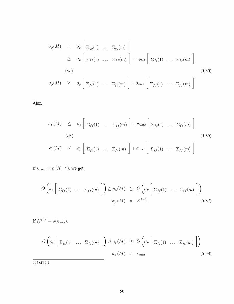
σp(M) = σp
[Σyy(1) . . . Σyy(m)
]≥ σp
[Σff (1) . . . Σff (m)
]− σmax
[Σfε(1) . . . Σfε(m)
](or) (5.35)
σp(M) ≥ σp
[Σfε(1) . . . Σfε(m)
]− σmax
[Σff (1) . . . Σff (m)
]
Also,
σp (M) ≤ σp
[Σff (1) . . . Σff (m)
]+ σmax
[Σfε(1) . . . Σfε(m)
](or) (5.36)
σp(M) ≤ σp
[Σfε(1) . . . Σfε(m)
]+ σmax
[Σff (1) . . . Σff (m)
]
If κmax = o(K1−δ), we get,
O
(σp
[Σff (1) . . . Σff (m)
])≥ σp(M) ≥ O
(σp
[Σff (1) . . . Σff (m)
])σp (M) � K1−δ. (5.37)
If K1−δ = o(κmin),
O
(σp
[Σfε(1) . . . Σfε(m)
])≥ σp(M) ≥ O
(σp
[Σfε(1) . . . Σfε(m)
])σp (M) � κmin (5.38)
363 of [5])
50

Thus, from (5.37) and (5.38) we get (5.30). Also,
σ1(M) = σ1
[Σyy(1) . . . Σyy(m)
]≥ σ1
[Σff (1) . . . Σff (m)
]− σmax
[Σfε(1) . . . Σfε(m)
](5.39)
(or)
σ1 (M) ≥ σ1
[Σfε(1) . . . Σfε(m)
]− σ1
[Σff (1) . . . Σff (m)
]
and following the same arguments as above, we get
σ1 (M) � max(κmax, K
1−δ) .Now, Frobenius norm of ∆M is given by,
‖∆M‖F =
∥∥∥∥ ∆Σyy(1) . . . ∆Σyy(m)
∥∥∥∥F
≤ ‖∆Σyy(1)‖F + . . .+ ‖∆Σyy(m)‖F (5.40)
where
‖∆Σyy(l)‖F ≤ √p ‖∆Σfε(l)‖F + p ‖∆Σff (l)‖F +
√p ‖∆Σεf (l)‖F + ‖∆Σεε(l)‖F
= OP
(K1− δ
2N−12
)+OP
(K1−δN−
12
). . . +OP
(K1− δ
2N−12
)+OP
(KN−
12
)= OP
(KN−
12
). (5.41)
51

Thus, substituting (5.41) in (5.40),
‖∆M‖F = OP
(KN−
12
). (5.42)
Note that ‖∆M‖2 also has the same convergence rate as shown in [22]. Now,
σp(M) + σmax(∆M) ≥ σp(M) ≥ σp(M)− σmax(∆M) (5.43)
and
σ1 (M)− σmax (∆M) ≥ σ1
(M)≥ σ1 (M)− σmax (∆M) (5.44)
upon substituting (5.30), (5.31) and (5.32) in (5.43) and (5.44), (5.33) and (5.34) is got.
Now proceeding to prove the Theorem:
Proof. When using HYBRID-III on M , (5.28), to get a decomposition as given in (5.9), the fol-
lowing inequalities are satisfied:
σmin
(R
(p)11
)≥
σp
(M)
√p (K − p+ 1)
(5.45)
and
σmax
(R
(p)22
)≤ σp+1
(M)√
(p+ 1) (K − p). (5.46)
Refer to Section 11 in [7] for a justification of these inequalities. Note HYBRID-III is applied on
M assuming a numerical rank p. From (5.33) in lemma 5.4, under the constraint Kδ√N
= o(1),
52

σmin
(R
(p)11
)≥
OP
(K1−δ√p(K−p+1)
), if κmax = o
(K1−δ)
OP
(κmin√
p(K−p+1)
), if o (κmin) = K1−δ
(5.47)
≥
OP
(K0.5−δ) , κmax = o
(K1−δ)
OP
(κmin√K
), o (κmin) = K1−δ
. (5.48)
Equation (5.46) and
σp+1
(M)≤ σp+1 (M) + ‖∆M‖2 ,
≤ ‖∆M‖2 as,σp+1(M) = 0
implies
∥∥∥R(p)22
∥∥∥2≤ ‖∆M‖2O
(√K).
Using (5.32), ∥∥∥R(p)22
∥∥∥2
= OP
(K
32N−
12
)(5.49)
Hence from (5.48) and (5.49), under the constraint
K1+δ
√N
= o(1),
oP
(σmin
(R
(p)11
))=∥∥∥R22
∥∥∥2
53

is satisfied.
Note for the matrix M , σmin(R
(p)11
)>∥∥∥R(K−p)
22
∥∥∥2
= 0, implying that p is a valid numerical
rank. Nevertheless, it is quite possible that σmin(R
(p−1)11
)>∥∥∥R(K−p−1)
22
∥∥∥2, implying the non-
uniqueness of a numerical rank. In the case of M determining p is simple as the last K − p rows
of the R matrix are zeros. In the case of M , an estimate p that maximizes the ratio
ri =γi + ε
γi+1 + ε, i = 1, 2, . . . , K (5.50)
where ε = γ1√KN
is as mentioned in (1.13) is used. The following theorem shows that for large
values of N , p is equal to p with a very high probability.
Theorem 5.2. Let M as in (1.4) be of rank ′p′ and let QR decomposition of MΠ be as in (1.12)
where Π is the permutation matrix got by HYBRID-III decomposition. Define γi as the ith diagonal
value of R in (1.12). Under the assumptions (A1-A7), refer Chapter 3 regarding assumptions, the
following properties hold true as K, N →∞ under the constraint Kδ√N
= o(1) regarding the ratio
(5.50).
Let UB (ri) and LB (ri) denote the upper and lower bounds for rate of growth of rias K,N →
∞.
54

Case1. for i = 1, p 6= 1 ,
UB (r1) =
OP
(√K), κmax = o
(K1−δ)
OP
(κmaxκmin
√K), o (κmin) = K1−δ
LB (r1) =
O(
1√K
), κmax = o
(K1−δ)
O(
κmaxκmin
√K
), o (κmin) = K1−δ
(5.51)
Case2. for 2 < i < p,
UB({ri}p−1
i=2
)= OP (K) ,
LB({ri}p−1
i=2
)= OP
(K−1
), (5.52)
Case3. for i = p,
UB (rp) = OP
(NK2
)LB (rp) =
OP
(K−(1+δ)N
12
), κmax = o
(K1−δ)
OP
(κminN
12K−2
), o (κmin) = K1−δ
(5.53)
55
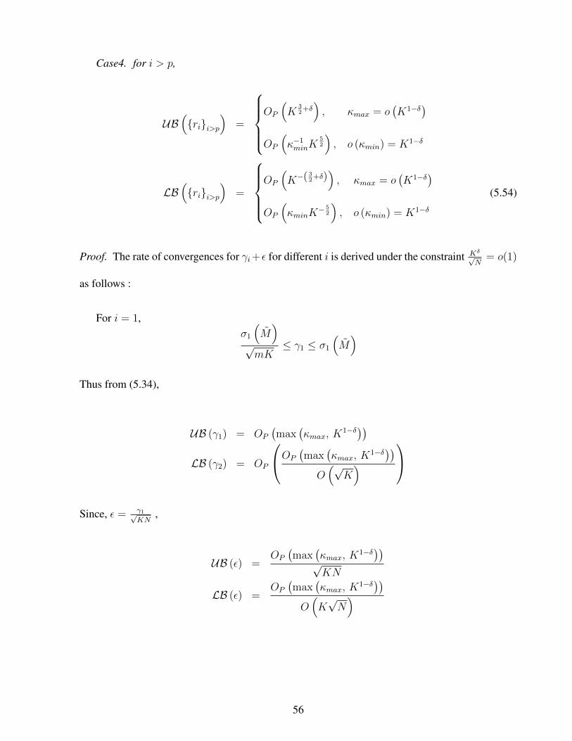
Case4. for i > p,
UB({ri}i>p
)=
OP
(K
32
+δ), κmax = o
(K1−δ)
OP
(κ−1minK
52
), o (κmin) = K1−δ
LB({ri}i>p
)=
OP
(K−( 3
2+δ)), κmax = o
(K1−δ)
OP
(κminK
− 52
), o (κmin) = K1−δ
(5.54)
Proof. The rate of convergences for γi+ε for different i is derived under the constraint Kδ√N
= o(1)
as follows :
For i = 1,σ1
(M)
√mK
≤ γ1 ≤ σ1
(M)
Thus from (5.34),
UB (γ1) = OP
(max
(κmax, K
1−δ))LB (γ2) = OP
OP
(max
(κmax, K
1−δ))O(√
K)
Since, ε = γ1√KN
,
UB (ε) =OP
(max
(κmax, K
1−δ))√KN
LB (ε) =OP
(max
(κmax, K
1−δ))O(K√N)
56
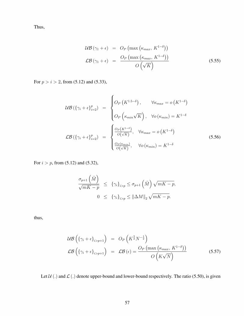
Thus,
UB (γ1 + ε) = OP
(max
(κmax, K
1−δ))LB (γ1 + ε) =
OP
(max
(κmax, K
1−δ))O(√
K) (5.55)
For p > i > 2, from (5.12) and (5.33),
UB ({γi + ε}pi=2) =
OP
(K1.5−δ) , ∀κmax = o
(K1−δ)
OP
(κmin√K), ∀o (κmin) = K1−δ
LB ({γi + ε}pi=2) =
OP (K1−δ)O(√K)
, ∀κmax = o(K1−δ)
OP (κmin)
O(√K)
, ∀o (κmin) = K1−δ
(5.56)
For i > p, from (5.12) and (5.32),
σp+1
(M)
√mK − p
≤ {γi}i>p ≤ σp+1
(M)√
mK − p,
0 ≤ {γi}i>p ≤ ‖∆M‖2
√mK − p.
thus,
UB({γi + ε}i>p+1
)= OP
(K
32N−
12
)LB({γi + ε}i>p+1
)= LB (ε) =
OP
(max
(κmax, K
1−δ))O(K√N) (5.57)
Let U (.) and L (.) denote upper-bound and lower-bound respectively. The ratio (5.50), is given
57
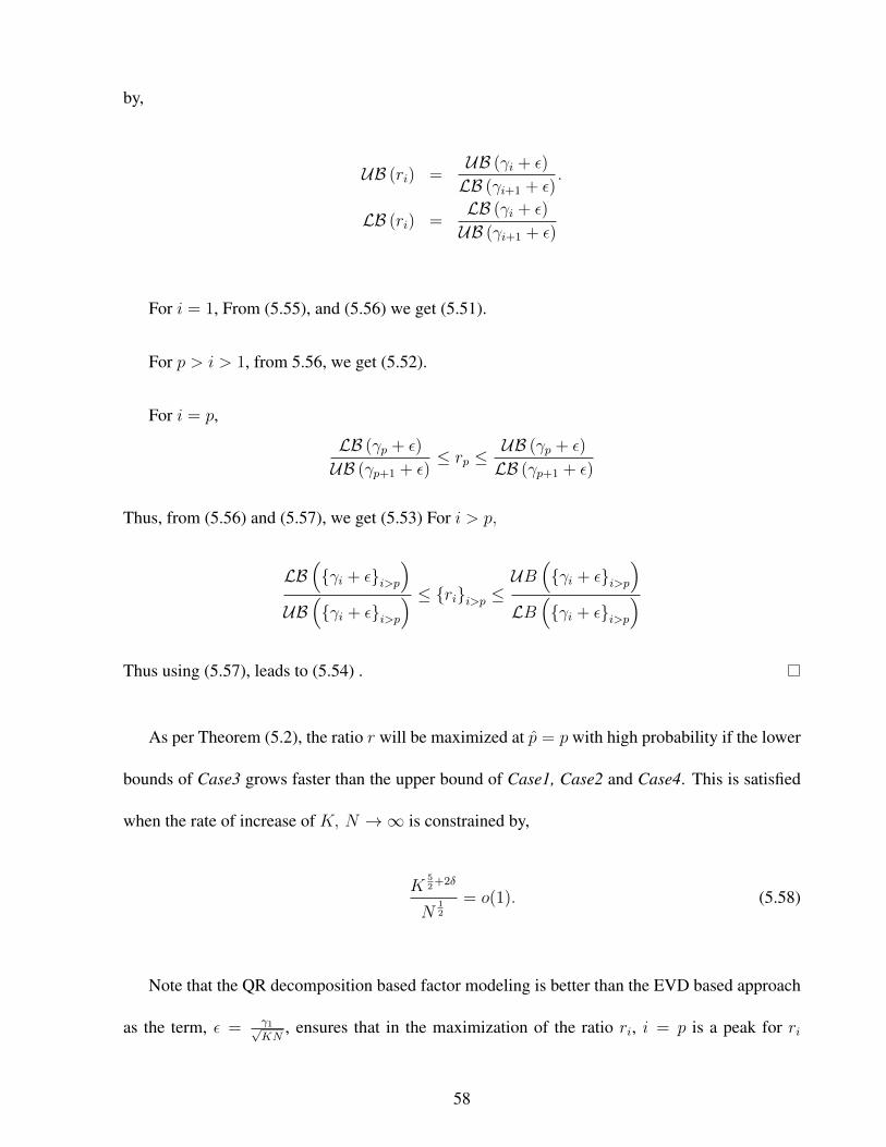
by,
UB (ri) =UB (γi + ε)
LB (γi+1 + ε).
LB (ri) =LB (γi + ε)
UB (γi+1 + ε)
For i = 1, From (5.55), and (5.56) we get (5.51).
For p > i > 1, from 5.56, we get (5.52).
For i = p,
LB (γp + ε)
UB (γp+1 + ε)≤ rp ≤
UB (γp + ε)
LB (γp+1 + ε)
Thus, from (5.56) and (5.57), we get (5.53) For i > p,
LB({γi + ε}i>p
)UB({γi + ε}i>p
) ≤ {ri}i>p ≤ UB({γi + ε}i>p
)LB
({γi + ε}i>p
)Thus using (5.57), leads to (5.54) .
As per Theorem (5.2), the ratio r will be maximized at p = p with high probability if the lower
bounds of Case3 grows faster than the upper bound of Case1, Case2 and Case4. This is satisfied
when the rate of increase of K, N →∞ is constrained by,
K52
+2δ
N12
= o(1). (5.58)
Note that the QR decomposition based factor modeling is better than the EVD based approach
as the term, ε = γ1√KN
, ensures that in the maximization of the ratio ri, i = p is a peak for ri
58

whereas ri at i = p is just a knee point in the EVD based model order determination.
59
Chapter 6
Perturbation Analysis of Q
In this Chapter, M as defined in (1.11) is treated as the perturbed version of M (1.4). Let
∆M , M −M
,
[∆Σyy(1) ∆Σyy(2) . . . ∆Σyy(m)
](6.1)
and ∆Σyy(l) denote the perturbation in M and Σyy(l) respectively. Also, Q got from MΠ is taken
as the perturbed version of Q got from MΠ, where Π is any permutation matrix. Assumption
(A5) implies that MΠ converges to MΠ as N → ∞ (for a fixed K), refer to Theorem 27.4 in
[6]. Thus Q should go to Q as N → ∞. Therefore, the search is for a permutation Π that renders∥∥∥Q−Q∥∥∥ reasonably small for a finite N . As mentioned earlier, here a unique Π is determined
using HYBRID-I RRQR algorithm. This choice is justified in Section 6.1. In Section 6.2, the con-
vergence rate of∥∥∥Q−Q∥∥∥
Ffor the proposed algorithm along with a measure of the convergence
rate of factors, fn is presented.
6.1 Perturbation analysis of QR decomposition:
Let, Mp denote the first p columns selected from MΠ as mentioned in (1.12) and Mp, ∆Mp
denote the first p columns selected from MΠ and ∆MΠ respectively. Thus,
Mp = Mp + ∆Mp. (6.2)

Consider the following two lemmas taken from [8]:
Lemma 6.1. Let Mp ∈ RK×p be of full column rank, p, then: Mp + ∆Mp is also of rank p if,
σmin(Mp) > σmax(P1∆Mp) (6.3)
where, P1 is the projection matrix that projects ∆Mp toR(Mp).
Proof. Refer to [8] for a proof.
Lemma 6.2. Let Mp ∈ RK×p be a matrix of rank p, with the QR decomposition Mp = Q1R and
∆Mp be the perturbation on Mp such that Mp + ∆Mp is also of rank p. Mp + ∆Mp has unique
QR factorization:
Mp + ∆Mp = (Q1 + ∆Q1) (R + ∆R)
where,
‖∆Q1‖F ≤√
2‖∆Mp‖Fσmin(Mp)
+O(ε2)
(6.4)
and
ε =‖∆Mp‖F‖Mp‖2
.
Proof. Refer to [8] for a proof.
Note that in the current context ‖∆Q1‖F =∥∥∥Q−Q∥∥∥
F. Lemmas 1 and 2 suggest choosing a
permutation matrix Π such that σmin (Mp) is maximized. Maximizing σmin(Mp) is equivalent to
61
maximizing σmin(Mp
)as
σmin (Mp) ≥ σmin
(Mp
)− σmax (∆Mp) .
HYBRID-I RRQR algorithm [7] selects a Π by trying1 to maximize σmin(Mp
). The effect of
using HYBRID-I algorithm of RRQR is presented in Theorem 4
Theorem 6.1. Let M ∈ RK×mK . Then the HYBRID-I RRQR algorithm could be used to select a
Π such that the first ′p′ columns from MΠ, Mp, satisfies
σp
(M)≥ σmin(Mp) ≥
σp(M)√p(K − p+ 1)
(6.5)
Proof. Applying Hybrid I algorithm [7] to M , leads to a permutation matrix Π given by (1.12),
where,
σmin(R11) ≥ σp(R)√p(K − p+ 1)
(6.6)
Refer to [7] for a complete proof. Select Mp as the first p columns of MΠ. QR decomposition of
Mp gives,
Mp = Qp R11.
Hence,
σmin
(Mp
)= σmin
(R11
). (6.7)
1To get a Π that maximizes σmin(Mp
)is a NP-hard problem and applying a brute force method would require
finding σmin(Mp
)for KmCp matrices where Km is the total number of columns in M . HYBRID-I RRQR is a
computationally simpler technique that generates a permutation Π which satisfies (6.5)
62
Interlacing property of singular values, [14, 25], ensures,
σp
(M)≥ σmin
(Mp
). (6.8)
Thus, (6.6), (6.7) and (6.8) leads to (6.5).
Henceforth, the term RRQR is used to refer the HYBRID-I RRQR algorithm for simplicity. In
the next subsection, convergence of Q to Q, obtained by using the RRQR on M and M respec-
tively, as N, K →∞ is investigated.
6.2 Convergence Analysis of Q
The rate of convergence of Q to Q as N, K →∞ is summarized in the following theorem:
Theorem 6.2. Under the conditions (A1-A7), refer Chapter 3 regarding assumptions, with the
optimistic assumption that the upper bound is achieved in (6.5) and with rate of increase of K and
N constrained by Kδ
N= o(1), the following convergence rate for Q is got:
∥∥∥Q−Q∥∥∥F�
OP
(K
δ2N−
12
), κmax = o
(K1−δ)
OP
(κ−1minK
1− δ2N−
12
), K1−δ = o (κmin)
(6.9)
and in the worst case scenario of (6.5), where the lower-bound of (6.5) is taken, under the con-
straint K1+δ
N= o(1),
∥∥∥Q−Q∥∥∥F�
OP
(K
1+δ2 N−
12
), κmax = o
(K1−δ)
OP
(κ−1minK
3−δ2 N−
12
), K1−δ = o (κmin)
(6.10)
63
Proof. The perturbation on Q is given by (6.4). Let, Mp denote the first p columns selected from
MΠ as mentioned in (1.12) andMp, ∆Mp denote the first p columns selected fromMΠ and ∆MΠ
respectively. Then,
Mp = Mp + ∆Mp. (6.11)
According to (6.3), The following equation needs to be satisfied:
σmin
(Mp
)> σmax (∆Mp) .
According to (6.5),
σp(M) ≥ σmin
(Mp
)≥ σp(M)√
p (K − p+ 1)(6.12)
Thus according to (5.33) and (6.12), The best estimate of σp(Mp
)is given by,
σmin
(Mp
)�P
K1−δ , if κmax = o
(K1−δ)
κmin , if o (κmin) = o(K1−δ) , ∀
Kδ
√N
= o(1). (6.13)
and in the worst case scenario,
σmin
(Mp
)�P
K1−δ√K
, if κmax = o(K1−δ)
κmin√K
, if o (κmin) = o(K1−δ) , ∀
Kδ
√N
= o(1). (6.14)
Note that ∆Mp are p columns selected from ∆MΠ. Using (5.40) and (5.41) it can be inferred that
64
O (‖∆M‖F ) = O (∆Σyy(l)). Let ∆Σ(p)yy (l) be p columns selected from ∆Σyy(l). Then,
‖∆Mp‖F � O(∆Σ(p)
yy (l))
≤ O(∥∥∥∆Σ
(p)fε (l)
∥∥∥F
)+O
(∥∥∥∆Σ(p)ff (l)
∥∥∥F
). . . (6.15)
. . . +O(∥∥∥∆Σ
(p)εf (l)
∥∥∥F
)+O
(∥∥∆Σ(p)εε
∥∥F
)
Note that∥∥∥∆Σ
(p)fε (l)
∥∥∥F≤ ‖∆Σfε(l)‖F ,
∥∥∥∆Σ(p)εf (l)
∥∥∥F≤ ‖∆Σεf (l)‖F and
∥∥∥∆Σ(p)ff (l)
∥∥∥F≤ ‖∆Σff (l)‖F .
From the proof of (5.23), it can be seen that ∆Σεε(l) is an uniform perturbation in all columns.
Thus, let ∆Σ(p)εε be the perturbation in p columns due to ∆Σεε(l) then
∥∥∆Σ(p)εε
∥∥F�P (Kp)
12 N
12
�P K12N
12 . (6.16)
Thus substituting (5.20), (5.21), (5.22) and (6.16) in (6.15) leads to
‖∆Mp‖F ≤ OP
(K1− δ
2N−12
)+OP
(K1−δN−
12
)+OP
(K
12N−
12
)= OP
(K1− δ
2N−12
). (6.17)
Thus in the best case scenario (6.13), under the constraint Kδ√N
= o(1), (6.3) is satisfied with high
probability as
o(σmin
(Mp
))= ‖∆Mp‖F .
Similarly in the worst case scenario, from (6.14) and (6.17), it can be shown that under the condi-
tion K1+δ2√N
= o(1), lemma 1 is satisfied with high probability.
65
In order to estimate ‖∆Q‖F as given by (6.4), σmin (Mp) has to be estimated. Note
σmin
(Mp
)+ σmax (∆Mp) ≥ σmin (Mp) ≥ σmin
(Mp
)− σmax (∆Mp) . (6.18)
Now, σmax (∆Mp) ≤ ‖∆Mp‖F thus substituting, (6.13) and (6.17) in (6.18), for the optimistic
scenario,
σmin (Mp) �P
K1−δ , if κmax = o
(K1−δ)
κmin , if o (κmin) = o(K1−δ) , ∀
Kδ
N= o(1). (6.19)
and in the worst case scenario substituting (6.14) and (6.17) in (6.18),
σmin (Mp) �P
K1−δ√K
, if κmax = o(K1−δ)
κmin√K
, if o (κmin) = o(K1−δ) , ∀
K1+δ
N= o(1). (6.20)
In the optimistic viewpoint, using (6.19) and (6.17) in (6.4) leads to (6.9). Similarly for the worst
case scenario, substituting (6.17) and (6.20) in (6.4), leads to (6.10).
The following theorem determines the convergence rate of the estimated factors. This is similar
to Theorem 3 of [22]. Let
Y ,
[y1 y2 . . . yN
]F ,
[f1 f2 . . . fN
](6.21)
E ,
[ε1 ε2 . . . εN
].
The convergence of the factors are got as a measure of the convergence of the Root Mean Square
Error (RMSE) given by, (KN)−0.5∥∥∥QF −QF∥∥∥
F, where F is the estimated factors.
66
Theorem 6.3. Under the conditions (A1-A7), refer Chapter 3 regarding assumptions,
(KN)−0.5∥∥∥QF −QF∥∥∥
F≤ OP
(K−
δ2
∥∥∥Q−Q∥∥∥F
+K−12
)(6.22)
Proof. The RMSE error of the estimated Y = QF is given by, KN−12
∥∥∥QF −QF∥∥∥F
. Now,
[QF −QF
]=
[QQTQF − QQTE −QF
]=
[QQT − I
]QF − Q
[Q−Q
]TE + QQTE
= K1 +K2 +K3
where, K1 =[QQT − I
]QF , K2 = Q
[Q−Q
]TE, K3 = QQTE. Now,
K1 =[QQT − I +QQT −QQT
]QF
=[QQT −QQT
]QF −
[I −QQT
]QF
Note,[I −QQT
]is a projection matrix onto the null space of Q hence,
[I −QQT
]QF = 0.
Hence,
K1 =[QQT −QQT
]QF (6.23)
Now using Q = Q+ ∆Q,
[QQT −QQT
]=
[∆Q∆Q> +Q∆Q> + ∆QQ>
]
67

hence,
∥∥∥QQT −QQT∥∥∥F≤ ‖∆Q‖2
F +∥∥Q∆Q>
∥∥F
Thus,
‖K1‖F = O (‖∆Q‖F ‖F‖F )
Substituting (5.24),
∥∥∥QQT −QQT∥∥∥F≤ O (‖∆Q‖F )O
(K
1+δ2 N
12
)(6.24)
Now,
‖K2‖F =
∥∥∥∥Q [Q−Q]T E∥∥∥∥F
≤∥∥∆QTE
∥∥F≤∥∥∆QT
∥∥F‖E‖2
also,
‖K3‖F =∥∥∥QQTE
∥∥∥F
≤∥∥QTE
∥∥F
≤
(N∑n=1
j=p∑j=1
(qTj εn
)2
)0.5
Now consider the Random variable q>j εn where E{q>j εn
}= 0 and var
(q>j εn
)= qjΣεεq
>j ≤
σmax (Σεε) = c < ∞ where c is a constant independent of K, N according to assumption (A4).
68

Thus,
‖K3‖F ≤ p12N
12OP (1).
Since∥∥∆QT
∥∥F
= oP (1) and ‖Q‖F =√p, ‖K2‖F is dominated by ‖K3‖F in probability. Hence,
(KN)−12
∥∥∥Qf −Qf∥∥∥F≤ OP
(K−
δ2
∥∥∥Q−Q∥∥∥F
+K−12
).
69

This page is intentionally left blank
70

Chapter 7
Comparison with the EVD Method
In this Chapter, the proposed algorithm is compared against the EVD based algorithm proposed in
[22] with regards to the asymptotic properties derived in the previous Chapter.
The convergence of the estimate, QEV D ofQ got using the EVD algorithm and the correspond-
ing expressions for rate of convergence are presented in [22]. The following theorem is taken from
[22].
Theorem 7.1. Under the conditions A2-A7 and (A8),
(A8) There should be at least one Σxx(l) of full rank p.
and all the Eigen values of S (3.1) being distinct the following convergence rates hold,
∥∥∥QEV D −Q∥∥∥
2�
OP
(KδN−
12
),
κmax = o(K1−δ)
KδN−12 = o(1)
OP
(κ−2minκmaxKN
− 12
),
K1−δ = o (κmin)
κ−2minκmaxKN
− 12 = o(1)
(7.1)
Proof. Refer to [22] for a proof.
In the best case scenario, (6.9), the ratio of the convergence rates of the EVD algorithm vs. the
proposed RRQR algorithm is given by,
∥∥∥Q(EV D) −Q∥∥∥
2∥∥∥Q(RRQR) −Q∥∥∥F
�
K
δ2 , κmax = o
(K1−δ)
κmaxκmin
Kδ2 , o (κmin) = K1−δ
, (7.2)
and in the worst case scenario, (6.10), the ratio is given by,
∥∥∥Q(EV D) −Q∥∥∥
2∥∥∥Q(RRQR) −Q∥∥∥F
�
K−( 1−δ
2 ) , κmax = o(K1−δ)
κmaxκmin
√K
, o (κmin) = K1−δ
. (7.3)
It is evident from (7.2), the proposed algorithm performs better than the EVD algorithm in the best
case scenario. However in the worst case scenario (7.3), it is evident that EVD Algorithm would
perform better. To probe this comparison further, consider the following example:
Example 7.1. Consider a data model as in (1.1), with p = 2 and the factors given by
xn ,
[x
(1)n x
(2)n
]>(7.4)
where,
x(1)n = e(1)
n + α1e(1)n−1,
x(2)n = e(2)
n + α2e(2)n−2 (7.5)
with e(1)n and e(2)
n being N(0, 1) iid process independent of the measurement noise, εn ∼ N (0, I).
The factor loading matrix H =
[h1 h2
]is a K × 2 matrix, where h1 and h2 are orthogonal
with‖h1‖22 � K1−δ1 and ‖h2‖2
2 � K1−δ2 where 0 ≤ δ1 < δ2 ≤ 1. This is similar to the factor
72
strength assumption taken in [21].
Let the QR decomposition of H be given by,
H =
[Q1 Q2
] R11
0
where Q1 is the K × 2 matrix that spans the column space of H , Q2 is the K × (K − 2) matrix
which spans the perpendicular space of H and
R11 =
‖h1‖2 0
0 ‖h2‖2
.
Note that, since xn is independent of εn,
Σyy(l) = Q1R11Σxx(l)R>11Q
>1
Thus,
Σyy(1) = Q1
‖h1‖22 0
0 0
Q>1 (7.6)
Σyy(2) = Q1
0 0
0 ‖h2‖22
Q>1 (7.7)
73
Further more, it is assumed that o(K1−δ2
)= KN−
12 . It can be shown that
∥∥∥QEV D −Q∥∥∥
2� ‖h1‖2
2
‖h2‖42
OP
(KN−
12
)(7.8)
OP
(KN−
12
)‖h2‖2
2
≤∥∥∥QRRQR −Q
∥∥∥F≤
OP
(K
32N−
12
)‖h2‖2
2
(7.9)
Proof. In [22], it is seen that when using the EVD method,
∥∥∥Q−Q∥∥∥2∝∥∥∆(MM>)∥∥
2
σp (MM>). (7.10)
For the current example, from (7.6) and (7.7),
σp(MM>) = ‖h2‖4
2 . (7.11)
Also it holds that,
∥∥∆(MM>)∥∥
2≤
∥∥M∆M>∥∥2
+∥∥∆MM>∥∥
2+∥∥∆M∆M>∥∥
2
= O(∥∥M∆M>∥∥
2
)= O (‖M‖2 ‖∆M‖2) (7.12)
and substituting from (5.32) and (7.6) in (7.12) leads to,
∥∥∆(MM>)∥∥
2� ‖h1‖2
2OP
(KN−
12
). (7.13)
Thus, substituting (7.11) and (7.13) in (7.10) the convergence rate for the EVD method is got as
74

(7.8). The convergence rate for QR decomposition is given by (6.4). Note from (7.7),
σ2 (M) = ‖h2‖22 .
Now, from (5.32) and (5.43), under the condition o(‖h2‖2
2
)= KN−
12 ,
σ2
(M)�P ‖h2‖2
2 .
and from (6.5),
‖h2‖22 ≥ σ2
(M2
)≥ ‖h2‖2
2√K
.
Thus, from (6.17) and (6.18),
‖h2‖22 ≥ σ2 (M2) ≥ ‖h2‖2
2√K
finally, applying (6.17) and the upper and lower bounds for σ2 (M2) in (6.4), (7.9) is obtained.
Thus the ratio of the convergence rates is given by,
O(Kδ2−δ1
)≤
∥∥∥QEV D −Q∥∥∥
2∥∥∥QRRQR −Q∥∥∥F
≤ OP
(Kδ2−δ1− 1
2
)(7.14)
Thus, In the best case scenario, the proposed algorithm is better by a factor of O(Kδ2−δ1
)and
in the worst case scenario the convergence rate is OP
(Kδ2−δ1− 1
2
), where δ2 > δ1. Thus if,
δ2 − δ1 >12, then even in the worst case, convergence rate of the proposed algorithm is better than
that of the EVD algorithm.
75

This page is intentionally left blank
76
Chapter 8
Illustration and Simulations:
Numerical illustrations of the proposed algorithm are presented in this Chapter. Here, four nu-
merical examples are considered. As the original motivation for this work comes from ([22]), a
simulation example presented therein is considered first. The results obtained by using the pro-
posed algorithm is compared with the EVD algorithm proposed in ([22]). The second problem
considered here is the simulation of Example 7.1 presented in Chapter 7. The results of the perfor-
mance of the proposed algorithm, the EVD and the PCA ([4]) are compared. In the third example,
a new algorithm is proposed for the separation of multiple audio signals from noisy mixtures. The
new algorithm is a conjunction of the proposed RRQR algorithm and the Independent Component
Analysis (ICA) technique. The presented algorithm has better noise characteristics when com-
pared to the conventional Noisy ICA technique ([17]). Finally, the proposed algorithm is applied
to model the US stock market data in comparison with the PCA based model.
8.1 Simulation 1
This simulation is used to illustrate the rate of convergence of Q to Q for the RRQR algorithm
in comparison with the EVD method. Consider (1.1) with a factor loading matrix
H =
[2 cos
(2πK
)2 cos
(4πK
). . . 2 cos (2π)
]>, (8.1)
the factors xn being generated by
xn = 0.9xn−1 + ηn, (8.2)

where process noise ηn and measurement noise εn are Gaussian noises with mean zero and variance
4. Data sets were generated using (1.1), (8.1) and (8.2) for K = 20, 180, 400 and 1000 and data
length N = 200 and 500.
Matrix M , (1.11), is generated for each pair (K,N) with m = 5. The L2 norm of the error
‖ Qi − Q ‖, i = 1, 2, is tabulated in Table 8.1. Here Q1 and Q2 are the estimates obtained using
EVD and RRQR methods respectively. Figure (8.1) shows the convergence of∥∥∥Q−Q∥∥∥
Ffor
RRQR and EVD methods with K = 60 while varying N for two different deltas, δ = 0 given by
(8.1), and δ = 0.5 given by
H1 =
[H(1 : K
2) Z
]T.
where Z is a vector of K2
zeros. It was noted that there was not much change in the observation
when varying K hence was neglected.
Assuming a fixed N = 100 and K = 180 in the above model, using 100 monte carlo trials, the
mean and standard deviation of the ratio, (3.5),
ri =λiλi+1
used in detecting the model order in the EVD method is plotted in figure 8.2. While the mean and
standard deviation of the ratio, (1.13),
ri =γi + ε
γi+1 + ε,
proposed for determining the model order using RRQR decomposition is plotted in figure 8.3.
78

Table 8.1: Summary of the results of Simulation 1,all values multiplied by 1000.K ‖ Q1 −Q ‖ ‖ Q2 −Q ‖ ‖ Q1 −Q ‖ ‖ Q2 −Q ‖
N = 200 N = 500
20 15.9 11.8 14.9 10.9180 17.4 12.3 15.9 11.3400 18 12.1 16.5 11.2
1000 18 12.3 11.6 11.4
Figure 8.1: Convergence of∥∥∥Q−Q∥∥∥
Ffor EVD and RRQR for fixed K = 60
From figure 8.2 and 8.3, it can be seen that the RRQR based model order detection scheme works
as good as EVD even when K � N . Also, it can be seen from the error bar that the proposed
RRQR method has lesser standard deviation and hence more consistant when compared to the
EVD estimate.
79

Figure 8.2: Plot of ratio of eigen values of MM>, ri (3.5) , for fixed K = 180; N = 100.
Figure 8.3: Plot of ratio of diagonal values of R in MΠ = QR, ri, (1.13), where Π is got usingRRQR Method for fixed K = 180; N = 100.
80

8.2 Simulation 2
Consider the data model given by (1.1) with the number of factors, p = 2 as in Example 1
and the factors xn taken as in (7.5) with α1 = 0.5 and α2 = 0.5. The factor strengths are taken
as δ1 = 0 and δ2 = 0.5 with the elements of the columns of H given by h1 ∼ U(−4, 4) and
h2
(1 : K
2
)∼ U(−4, 4) and h2
(K2
+ 1 : K)
= 0. Two scenarios are considered for the random
noise εn in (1.1). Firstly, εn is taken to be generated by N(0, I), I ∈ RK×K is an identity matrix.
In the second scenario, εn is taken as N(0, 0.1Σ), where the elements of Σ ∈ RK×K are given by
σi,j =1
2
(|i|2w − |i− j|2w + |j|2w
), (8.3)
where w, the Hurst parameter, is taken as 0.6.
The data sets were simulated for all pairs of (K, N) where K takes values of 100, 200, 400
and N takes, 100, 200. The simulated data set was run against the QR-PC algorithm, the EVD
algorithm and also the PCA algorithm proposed in ([4]). In ([4]), the model order is the p that
minimizes the Information Content,
ICp = ln(V (p, fn)
)+ p
(K +N
KN
)ln
(KN
K +N
)
where
V (p, fn) = minQ
1
KN
N∑n=1
∥∥∥yn − Q(p)f (p)n
∥∥∥2
2
Here, Q(p) and f (p)n are obtained using PCA by assuming model order as p. Thus, the estimate of
81
model order is
pN,K = arg minp{ICp}.
The Root Mean Square Error (RMSE) and Forecast Error (FE) were observed for all pairs (K, N)
and the mean over 100 montecarlo runs are tabulated. The RMSE error is
εrmse =
∑Nn=1
∥∥∥QN,K fn −Hxn∥∥∥
2
KN
0.5
(8.4)
and the mean FE given by
εfe =1
N
N∑n=1
(K−0.5
∥∥y(1)n − yn
∥∥2
), (8.5)
where y(1)n is the one step ahead forecast of yn got by using y(1)
n = QN,K f(1)n and f (1)
n is the one
step ahead forecast of the factors got by fitting AR model to factors using Yule-Walker algorithm.
The results are summarized in TABLE 8.2.
It could be noted that while the PCA method is better at estimating the RMSE error, the EVD
and proposed methods perform better when FE is concerned. Also, the proposed method performs
better than the EVD in certain cases. It could be noted that when ε ∼ N(0, I), all the three
algorithms were able to detect the correct model order. However when ε ∼ N (0, Σ), only the
EVD and RRQR methods were able to detect the model order correctly, while PCA overestimated
the model order by a huge difference. Finally it could also be noted that the number of lags, m,
considered is increased, the performance of the EVD and RRQR methods increased.
82

Table 8.2: Summary of Observations from Simulation 2. The RMSE and FE values are multipliedby 1000.
Noise I. εn ∼ N(0, I) II. εn ∼ N(0, 0.1Σ)K 100 100 100 200 200 200 100 100 100 200 200N 100 200 300 100 200 300 100 200 300 200 300
RRQR,m = 2
p 2 2 2 2 2 2 2 2 2 2 2εfe 1474 1486 1460 1465 1481 1480 1244 1230 1226 1250 1238εrmse 52.8 23.0 16.2 37.9 22.7 15.4 138 80 16 103 26.0
RRQR,m = 9
p 2 2 2 2 2 2 2 2 2 2 2εfe 1479 1479 1482 1481 1489 1482 1229 1229 1238 1227 1231εrmse 45.2 23.5 15.9 31.1 22.3 15.4 214 126 53.2 15.6 45.3
EVD,m = 2
p 2 2 2 2 2 2 2 2 2 2 2εfe 1475 1488 1464 1467 1484 1483 1241 1229 1226 1250 1239εrmse 40.1 20.7 14.5 26.5 19.7 13.3 113 79.5 14.1 109 54.0
EVD,m = 2
p 2 2 2 2 2 2 2 2 2 2 2εfe 1477 1480 1487 1476 1491 1484 1226 1230 1238 1229 1233εrmse 34.5 19.6 14.1 22.9 18.2 13.0 189 105 27.5 186 94.8
PCAp 2 2 2 2 2 2 18 22 24 29 33εfe 1470 1484 1461 1455 1477 1479 1243 1229 1238 1249 1238εrmse 19.9 12.2 9.4 11.2 10 7.4 107.2 75.8 61.9 114.7 93.6
8.3 Simulation 3 (ICA Pre-processing)
The Independent Component Analysis, ([9, 18]), is a well known technique for estimating the
factors. The basic ICA technique is used to extract p sources from p mixtures. When the mixtures
are noise corrupted and the number of such mixtures being larger than the total number of sources,
the Noisy ICA algorithm is used. The Noisy ICA ([17]) algorithm considers a model of the form,
yn = Wsn + εn (8.6)
where,
1. The factors, sn, are independent of each other.
2. Not more than one factor is Gaussian.
3. The factors sn are independent of εn.
83

4. The noise εn is Gaussian with co-variance σ2I , where I is an Identity matrix.
Given {yn}Nn=1, the Noisy ICA Algorithm estimates W and sn uniquely.
Here, an algorithm is developed by combining the proposed RRQR technique with the ba-
sic ICA algorithm. This helps in relaxing the conditions 3,4 presented above. The algorithm is
summarized below:
1. Obtain Q and fn from the mixtures, yn, as in data model (1.2) using the RRQR based tech-nique presented in Section 5.
2. Determine sn, A from fn such that,
sn , A−1fn
,[s
(1)n . . . s
(p)n
]>where A is a matrix obtained by using the basic ICA, such that the components of sn areindependent.
Thus,
yn = QAA−1fn + εn
Assuming W = QA,
yn = Wsn + εn (8.7)
Thus, W and sn could be extracted as in (8.7) under the following assumptions:
1. The components of sn are independent with each other.
2. Not more than one factor has Gaussian distribution.
3. All sn should have correlations with the past. i.e., E {sn+lsn} 6= 0 for at least one l =1, . . . ,m.
4. The random noise εn can be correlated with the factors sn, i.e., E {sn+lεn} need not neces-sarily be zero for all l ≥ 0.
84
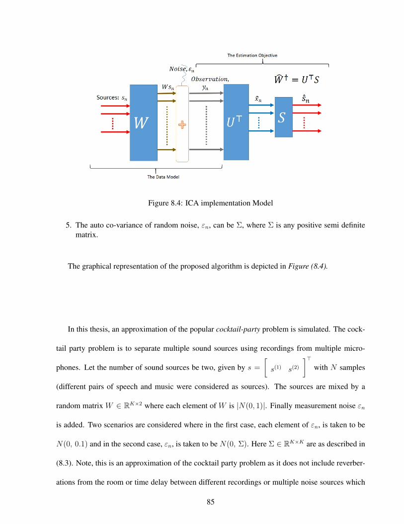
Figure 8.4: ICA implementation Model
5. The auto co-variance of random noise, εn, can be Σ, where Σ is any positive semi definitematrix.
The graphical representation of the proposed algorithm is depicted in Figure (8.4).
In this thesis, an approximation of the popular cocktail-party problem is simulated. The cock-
tail party problem is to separate multiple sound sources using recordings from multiple micro-
phones. Let the number of sound sources be two, given by s =
[s(1) s(2)
]>with N samples
(different pairs of speech and music were considered as sources). The sources are mixed by a
random matrix W ∈ RK×2 where each element of W is |N(0, 1)|. Finally measurement noise εn
is added. Two scenarios are considered where in the first case, each element of εn, is taken to be
N(0, 0.1) and in the second case, εn, is taken to be N(0, Σ). Here Σ ∈ RK×K are as described in
(8.3). Note, this is an approximation of the cocktail party problem as it does not include reverber-
ations from the room or time delay between different recordings or multiple noise sources which
85
might exceed the number of microphones used. For a more detailed analysis of the cocktail party
problem refer, ([15]). The performance of the algorithm is evaluated using PESQ score ([30]). The
PESQ is a tool that compares the original signal sn with the recovered signal sn and it gives a best
score of 4.5 when both match exactly. The ICA algorithm used is from ([16]). Since the speech
and music sources have a super Gaussian distribution, The kurtosis is assumed positive and tanh
non-linearity is used as a measure of non gaussianity in the implementation of fast ICA.
It could be noted from the observations in Table 8.3 that, the RRQR based method performs
better in almost all cases. It could also be noted that in the first scenario of noise, where the same
magnitude of noise was included in each observation, as the number of observed mixtures (K)
increased, the separation was more accurate implying that information from the increased number
of mixtures was used to separate out the components. The second scenario is quite different, as the
number of observed mixtures increased, the noise variance also increased i.e., the noise variance
was proportional to the number of observations as can be seen from (8.3). Thus, with the increase
in the number of observed mixtures, the increase in the noise magnitude offset the increase in the
performance thus, with increase in K, decrease in the performance of the algorithm is seen. It
was also noted that the PCA based method of ([4]) was unable to determine the number of sources
under the second scenario and its estimate for the number of sources were between 20-30. Thus, in
the simulation, the number of sources were assumed to be 2 in this case while using PCA. The EVD
and the proposed method did not suffer from this problem and were able to estimate the number of
sources as 2 quite consistently. It is also interesting to note that while speech-music separation was
the best, speech-speech separation was the worst. Thus, the separation characteristic also depends
on the type of source to be separated.
86

Source Type speech-speech speech-music music-musicK - Mixtures 10 40 100 10 40 100 10 40 100
(Average PESQ Score ) with εi, j ∼ N(0, 0.1)RRQR 2.282 2.813 3.1300 2.931 3.667 4.092 2.868 3.534 3.823EVD 2.275 2.780 3.1277 2.932 3.666 3.990 2.868 3.534 3.823PCA 2.285 2.812 3.1312 2.931 3.665 4.092 2.868 3.534 3.823
(Average PESQ Score ) with εn ∼ N(0,Σ)RRQR 3.515 3.088 2.670 4.261 4.017 3.695 4.221 4.006 2.835EVD 3.507 3.079 2.665 4.264 4.019 3.695 4.221 4.007 3.667PCA 4.064 4.086 3.956 3.886 3.581 3.386 3.887 3.355 3.667
Table 8.3: Errors Associated when used as pre-processing with ICA
8.4 Application on a finance portfolio
The proposed RRQR method, EVD and PCA were applied to model the returns of the S&P
500 index constituents. The S&P 500 is a diversified index that represents large companies in the
US. It is often taken as a representative index of the US market as a whole. We consider the 500
stocks that are members of the S&P Index as of July 31, 2013. We collect the data for these 500
stocks from January 1, 2010 - July 31, 2013. The prices are adjusted for splits and dividends. The
daily logarithmic returns are calculated from the adjusted prices. If P (n) and P (n − 1) are the
prices at time at n and n− 1, then the logarithmic return is:
yn = log (P (n))− log (P (n− 1)) .
Sixteen stocks did not have data for all days and hence were omitted from the study. The following
steps are applied to develop the factor models that are used to forecast the returns.
1. Let the total number of days be N and the number of stocks be K.
2. The mean across time is set to zero for all stocks, i.e.,
yn = yn − y, n = 1, 2, . . . , N.
where y = 1N
∑Nn=1 yn is the mean.
87
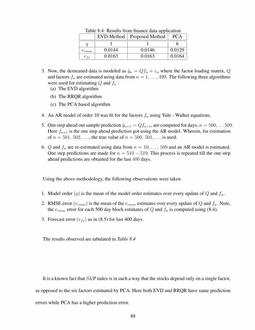
Table 8.4: Results from finance data applicationEVD-Method Proposed Method PCA
q 1 1 6ermse 0.0144 0.0146 0.0129efe 0.0163 0.0163 0.0164
3. Now, the demeaned data is modeled as yn = Qfn + εn where the factor loading matrix, Qand factors fn are estimated using data from n = 1, . . . , 499. The following three algorithmswere used for estimating Q and fn :
(a) The EVD algorithm
(b) The RRQR algorithm
(c) The PCA based algorithm
4. An AR model of order 10 was fit for the factors fn using Yule - Walker equations.
5. One step ahead out sample prediction yn+1 = Qfn+1, are computed for days, n = 500, . . . 509.Here fn+1 is the one step ahead prediction got using the AR model. Wherein, for estimationof n = 501, 502, . . ., the true value of n = 500, 501, . . . is used.
6. Q and fn are re-estimated using data from n = 10, . . . , 509 and an AR model is estimated.One step predictions are made for n = 510 − 519. This process is repeated till the one stepahead predictions are obtained for the last 400 days.
Using the above methodology, the following observations were taken
1. Model order (q) is the mean of the model order estimates over every update of Q and fn.
2. RMSE error (ermse) is the mean of the ermse estimates over every update of Q and fn. Note,the ermse error for each 500 day block estimates of Q and fn is computed using (8.4).
3. Forecast error (efe) as in (8.5) for last 400 days.
The results observed are tabulated in Table 8.4
It is a known fact that S&P index is in such a way that the stocks depend only on a single factor,
as opposed to the six factors estimated by PCA. Here both EVD and RRQR have same prediction
errors while PCA has a higher prediction error.
88

Chapter 9
Conclusion and Discussions
In this thesis, factor modelling of an observed K-dimensional multivariate series, yn, of length N
(n = 1, 2, . . . , N) was considered. The goal was to estimate a low p-dimensional series called
factors, fn (p < K) and a constant matrix Q such that yn = Qfn+εn, where εn was random noise.
The random noise was assumed to have covariance, Σεε(l) = Σδ(l), where Σ is a positive definite
matrix. It was also assumed that the factors can be correlated with past noise and not with future
noise i.e., Σfε(l) 6= 0 for l ≥ 0 and Σfε(l) = 0 for l < 0. In principle a “fat matrix”, M , can
be formed by augmenting the autocovariance matrices {Σyy(l)}ml=1. This matrix M would be of
rank p and span the same column space as Q i.e., R (M) = R (Q). Hence, determining p and Q
from SVD/QR decompositions of M is straight forward. In practice, only the finite time estimates
of the autocovariances are observed and hence only a perturbed version M of M is observable.
This matrix, M , would be full row rank with probability one. In this paper, the model order p
was determined by equating it to the “numerical rank” of the matrix M . The numerical rank of M
was determined by maximizing a ratio, (1.13), formed using the diagonal values of the R matrix
of the HYBRID-III RRQR decomposition, [7]. With the model order p determined, an estimate of
Q was obtained using HYBRID-I RRQR decomposition of M . The factors, fn, were obtained by
projecting the observations yn on the space spanned by the estimate of Q.
The HYBRID-III algorithm ensures that
σp
(M)√
(p+ 1) (K − p) ≥ σp
(Mp
)≥
σp
(M)
√p (K − p+ 1)
, (9.1)
were Mp denotes the first p columns selected from MΠ with Π being the permutation matrix
generated by the HYBRID-III algorithm. HYBRID-I and HYBRID-II algorithms satisfy the upper
and lower bounds, respectively, of (9.1). The above bounds were crucial for proving the asymptotic
convergence of the model order. In the simulations, QR-CP as well the other Hybrid algorithms
were found to to give similar results. Nevertheless, convergence results could be proved only for
Hybrid algorithms. In particular, convergence of the model order scheme could be proved only for
the Hybrid-III algorithm.
Conventional PCA based factor modelling cannot allow noise to be correlated with factors and
that noise should have covariance of Σεε(0) = σ2I . The proposed algorithm relaxes the above and
allows noise to have any covariance Σ. Thus it was seen from Simulations 8.2 and 8.3 that when
the noise had covariance anything other than σ2I , the PCA based model order detection schemes
[4] failed to detect the correct number of factors p, the proposed RRQR based scheme remained
robust.
The method of using M to determine the parameters in the factor model was first approached
by [22] wherein EVD of MM> was used to obtain estimates for p, Q and fn. It was proved that in
certain cases, the proposed RRQR based methodology is better than the EVD based method w.r.t
the asymptotic properties (as both the dimension and duration of observations, K and N , tends to
infinity). The numerical Simulations 8.1, 8.2 and 8.3 also demonstrate that RRQR betters EVD in
certain cases.
Using Example 1, it was shown that the factors might not have correlation at all lags and hence,
in order to acquire all factors, lags, l = 1, . . . ,m needs to be used withm high enough. Conversely,
it could be stated that using l = a, . . . , b where min (K,N) ≥ b ≥ a ≥ 1 to construct M would
result in the estimation of factors having correlation within those particular lags alone. This is
90

useful when, say, an a-step ahead prediction is desired (persistent factors) or if the undesirable
factors have correlation only in lags less than a.
The use of the proposed method of factor modelling as pre-processing to ICA was demon-
strated in Simulation 3. Finally, w.r.t the finance data application, the EVD method and the pro-
posed method perform similarly and identify only one dominant factor. This is expected since the
S&P 500 is a well diversified index and the only common factor among all the constituent stocks
is the US market factor.
This work can be extended to devise a recursive algorithm to estimate the parameters of the
factor model based on RRQR decomposition.
91

This page is intentionally left blank
92

Appendix 1
Interlacing Property
The following lemma relates to the interlacing property of eigen values for symmetric matrices:
Lemma 9.1. [25, 11]Let A be real symmetric matrix of dimension n and B ∈ Rk×k be a principal
sub matrix of A with 1 ≤ k < n. Let a1 ≥ a2 ≥ ... ≥ an and b1 ≥ b2 ≥ ... ≥ bk be the respective
eigenvalues. Then
aj ≥ bj ≥ an−k+j, j = 1, 2...k (9.2)
Proof. Refer [25] for a proof.
Theorem 9.1. Let Σ ∈ Rm×n, m < n, and Σk×l11 , k < l, be any sub matrix of Σ with σ1 ≥ σ2 ≥
. . . ≥ σm and λ1 ≥ λ2 ≥ . . . ≥ λk being their corresponding singular values. Then,
σj ≥ λj ≥ σn−k+j, j = 1, 2...k.
Proof. First we start by establishing the connection between the eigen values and singular values
so as to connect the result in the previous lemma to pertain to singular values. The following
properties are used:
93

1. Singular values of a matrix Σ ∈ Rm×n , m < n, are equal to the square roots of the eigen
values of the matrix A = Σ>Σ (or) ΣΣ>.
2. Also, let QR decomposition of Σ be, Σ = QR. Then singular values of R equals that of Σ,
σ1 ≥ σ2 ≥ . . . ≥ σm, since Q is an orthogonal matrix.
Let Σ11 ∈ Rk×l, k < l, be a principal sub matrix of Σ. Using the second property, without loss
of generality, Σ can be written as upper triangular, for the purpose of dealing with singular values,
i.e.,
Σ =
l n− l
k
m− k
Σ11 Σ12
0 Σ22
.
Also, let λ1 ≥ λ2 ≥ . . . ≥ λk be the singular values of Σ11. Now, Consider the symmetric matrix,
A , Σ>Σ given by,
A = Σ>Σ =
k n− k
k
n− k
Σ>11Σ11 Σ>12Σ12
Σ>12Σ12 Σ>22Σ22
.
Note, the symmetric matrix Σ>11Σ11 is a principal sub matrix ofA. Now, Lemma 9.1 can be applied
assuming B = Σ>11Σ11. Thus, the eigen values of Σ>Σ and Σ>11Σ11 are related as in (9.2). Thus
taking the positive square root of which would correspond to the singular values of Σ and Σ11.
Thus,
σj ≥ λj ≥ σn−k+j, j = 1, 2...k.
94

This above theorem is used in Chapters 4, 5 and 6.
95
Appendix 2
Landau notations and Mixing Properties
Properties of Order Notations (landau notations)
Here the properties of little o, big O, little oP and big OP are summarized. Refer also [24].
Properties of little o and big O:
1. an = O(an)
2. If an = o(bn), then an = O(bn)
3. If an = O(bn), then O(an) +O(bn) = O (an).
4. If an = O(bn), then o(an) + o(bn) = o(an)
5. Let c be a constant, then cO(an) = O(an) and co(bn) = o(bn).
6. O(an)O(bn) = O(anbn); o(an)o(bn) = o(anbn)
The properties of OP and oP are summarized as follows:
1. Let an be any stochastic sequence and bn be a deterministic sequence then, o (an) = bn
implies the stochastic sequence bnan
P→ 0.
96

while almost all the properties pertaining to O and o could be applicable to OP and oP , the follow-
ing two properties are not so obvious:
2. Let an and bn deterministic sequences, then, O (an) +OP (bn) = OP (an + bn) .
Proof. Let,
Cn = An +Xn
where An is a deterministic sequence and Xn is a random sequence. Let the rate of convergence
of Anand Xnbe as follows:
An = O (an)
Xn = OP (bn)
where an and bn are deterministic sequences. By definition of O(.) and OP (.),
∣∣∣∣Anan∣∣∣∣ ≤ M1 ∀n > n0
P
{∣∣∣∣Xn
bn
∣∣∣∣ ≤M2
}≥ 1− εn0 ∀n > n0
Thus,
Cn = O (an) +OP (bn)
=⇒ P
(∣∣∣∣Anan∣∣∣∣+
∣∣∣∣Xn
bn
∣∣∣∣ ≤M1 +M2
)≥ 1− εn0 ∀n > n0
=⇒ Cn = OP (an + bn)
97
if an > bn then,
Cn = OP (an) .
3. Let an and bn deterministic sequences, then, O (an)OP (bn) = OP (anbn) .
Proof. Let,
Cn = AnXn
where An is a deterministic sequence and Xn is a random sequence. Let the rate of convergence
of Anand Xnbe as follows:
An = O (an)
Xn = OP (bn)
where an and bn are deterministic sequences. By definition of O(.) and OP (.),
∣∣∣∣Anan∣∣∣∣ ≤ M1 ∀n > n0
P
{∣∣∣∣Xn
bn
∣∣∣∣ ≤M2
}≥ 1− εn0 ∀n > n0
Thus,
Cn = O (an)OP (bn)
=⇒ P
(∣∣∣∣Anan∣∣∣∣ ∣∣∣∣Xn
bn
∣∣∣∣ ≤M1M2
)≥ 1− εn0 ∀n > n0
=⇒ Cn = OP (anbn)
98
Mixing Conditions
In Chapter 2, the stationarity of the time series was due to the assumptions on the mixing
conditions namely, α (.) and ψ(.). Here an explanation pertaining to the same are summarized.
For more details refer [6, pp 363 - 367] and [10, sec 2.6].
To express dependency across time for an observed stochastic sequence, one could use the
Moving Average (MA) model. But it is too simplistic and cannot comply with complicated de-
pendence structures. Hence, mixing conditions are used. Mixing conditions state that that, across
time, two well separated instances are independent of each other. This enables the use of law of
Large Numbers and the Central Limit Theorem for a non-independent stochastic series.
Let X1, X2, . . . be a sequence of random variables. Now, α mixing is defined as,
αn = supA∈σ(X1, ..., Xk);B∈σ(Xk+n, Xk+n+1, ...)
|P (A ∩B)− P (A)P (B)|
where σ (X1, . . . , Xk) be the sigma algebra generated by X1, . . . , Xk. Also, the ψ mixing condi-
tion is given by
ψn = supA∈σ(X1, ..., Xk);B∈σ(Xk+n, Xk+n+1, ...)
∣∣∣∣1− P (B|A)
P (B)
∣∣∣∣ .Now, if αn → 0, then the random variables Xi and Xi+n are taken to be independent for large n
and the sequence is addressed as to have α−mixing. Note, if the mean and co-variance of Xn is
independent of n, then Xn is assumed to be stationary.
The following theorem is taken from Billingsley, [6, Thm 27.4]:
Theorem 9.2. Suppose X1, X2, . . . is stationary with αn = O(n−5), E (Xn) = 0 and E (X12n ) <
99
∞. Let
S ,N∑n=1
Xn,
then,
N−1Var (Sn)→ σ2 = E(X2
1
)+ 2
∞∑k=1
E (X1X1+k) ,
where the series converges absolutely. If σ > 0, then Snσ√N∼ N (0, 1).
Proof. Refer [6, Thm 27.4] for proof
This above theorem is important for numerous aspects as it implies that our M , (1.11), tends
to M , (1.4), as N → ∞ for fixed K. It also the gives the rate of growth for a sum of a series
satisfying the above conditions to be OP
(√N). This fact is used in deriving lemma (5.3).
In lemma (5.3), we obtained the matrix Σxε(l) − Σxε(l) where Σxε(l) is a sample covariance
matrix between xn and εn and Σxε(l) is their ideal co-variance matrix. Therein, xn and εn are
given by
yn = Hxn + εn.
where yn is the stochastic sequence, which satisfies the properties in Theorem 9.2 (Refer Condition
(A5) of Chapter 2). Since xn and εn are also linearly related to yn, they too satisfy those properties
ensuring that the every element in the matrix xn+lε>n − E
(xn+lε
>n
)also satisfy the conditions for
Theorem 9.2. Since every element in the matrix Σxε(l)−Σxε(l) = 1N
∑Nn=1
(xn+lε
>n − E
[xn+lε
>n
])correspond to the sum of the above sequence from n = 1 . . . N divided by N , they all converge at
the rate Op
(1√N
).
Note that α − mixing, also known as strong mixing, is weaker than ψ − mixing. Hence
100

ψ−mixing implies α−mixing. For more details regarding the property of ψ mixing, refer [10].
101

This page is intentionally left blank
102
Bibliography
[1] Hirotugu Akaike. Factor analysis and aic. Psychometrika, 52(3):317–332, 1987.
[2] T. W. Anderson. Asymptotic theory for principal component analysis. Ann. J. Math. Stat.,34:122–148, 1963.
[3] T.W. Anderson. The use of factor analysis in the statistical analysis of multiple time series.Psychometrika, 28(1):1–25, 1963.
[4] J. Bai and S. Ng. Determining the number of factors in approximate factor models. Econo-metrica, 70(1):191–221, 2002.
[5] Dennis S Bernstein. Matrix mathematics: theory, facts, and formulas. Princeton UniversityPress, 2009.
[6] Patrick Billingsley. Probability and measure. John Wiley & Sons, 2008.
[7] Shivkumar Chandrasekaran and Ilse CF Ipsen. On rank-revealing factorisations. SIAM Jour-nal on Matrix Analysis and Applications, 15(2):592–622, 1994.
[8] Xiao-Wen Chang, Christopher C Paige, and GW Stewart. Perturbation analyses for the qrfactorization. SIAM Journal on Matrix Analysis and Applications, 18(3):775–791, 1997.
[9] Pierre Comon. Independent component analysis, a new concept? Signal processing,36(3):287–314, 1994.
[10] Jianquing Fan. Nonlinear time series: nonparametric and parametric methods. Springer,2003.
[11] Ky Fan and Gordon Pall. Imbedding conditions for hermitian and normal matrices. Canad.J. Math, 9(195):7, 1957.
[12] W. Gander. Algorithms for the qr decomposition. Res. Rep, pages 80–02, 1980.
[13] Gene Golub, Virginia Klema, and Gilbert W Stewart. Rank degeneracy and least squaresproblems. Technical report, DTIC Document, 1976.
[14] Gene H Golub and Charles F Van Loan. Matrix computations, volume 3. JHU Press, 2012.
[15] Eugen Hoffmann, Dorothea Kolossa, and Reinhold Orglmeister. Recognition of multiplespeech sources using ica. In Robust Speech Recognition of Uncertain or Missing Data, pages319–344. Springer, 2011.
[16] A Hyvärinen et al. The fastica package for matlab. Helsinki Univ. of Technology, Espoo,Finland, 2005.
103
[17] Aapo Hyvärinen, Juha Karhunen, and Erkki Oja. Independent component analysis, vol-ume 46. John Wiley & Sons, 2004.
[18] Aapo Hyvärinen and Erkki Oja. Independent component analysis: algorithms and applica-tions. Neural networks, 13(4):411–430, 2000.
[19] K. G. Joreskog. A general approach to confirmatory maximum likelihood factor analysis.Psychometrika, 34(2), 1969.
[20] K. V. Mardia, J. T. Kent and J. M. Bibby. Multivariate Analysis. Academic Press, London,1979.
[21] C. Lam and Q. Yao. Factor modeling for high-dimensional time series: Inference for thenumber of factors. The Annals of Statistics, 40(2):694–726, 2012.
[22] C. Lam, Q. Yao, and N. Bathia. Estimation of latent factors for high-dimensional time series.Biometrika, 98(4):901–918, 2011.
[23] D.N. Lawley. The estimation of factor loadings by the method of maximum likelihood.Proceedings of the Royal Society of Edinburgh, 60(2), 1940.
[24] Erich Leo Lehmann. Elements of large-sample theory. Springer Verlag, 1999.
[25] Chi-Kwong Li, Yiu-Tung Poon, and Nung-Sing Sze. Generalized interlacing inequalities.Linear and Multilinear Algebra, 60(11-12):1245–1254, 2012.
[26] M. Wax and T. Kailath. Detection of signals by information theoretic criteria. IEEE Trans.Acoust., Speech, Signal Processing, 33:387–393, 1985.
[27] M. Wax, T. J. Shan, and T. Kailath. Spatio-temporal spectral analysis by eigenstructuremethods. IEEE Trans. Acoust., Speech, Signal Processing, 32:817–827, 1984.
[28] P. Stoica and M. Jansson. On maximum likelihood estimation in factor analysis an algebraicderivation. Signal Processing, 89:1260–1262, 2009.
[29] Jorma Rissanen. Modeling by shortest data description. Automatica, 14(5):465–471, 1978.
[30] Antony W Rix, John G Beerends, Michael P Hollier, and Andries P Hekstra. Perceptualevaluation of speech quality (pesq)-a new method for speech quality assessment of tele-phone networks and codecs. In Acoustics, Speech, and Signal Processing, 2001. Proceed-ings.(ICASSP’01). 2001 IEEE International Conference on, volume 2, pages 749–752. IEEE,2001.
[31] N.D. Sidiropoulos, R. Bro, and G.B. Giannakis. Parallel factor analysis in sensor array pro-cessing. Signal Processing, IEEE Transactions on, 48(8):2377–2388, 2000.
[32] Charles Spearman. The proof and measurement of association between two things. Americanjournal of Psychology, 15(1):72–101, 1904.
[33] GW Stewart. Rank degeneracy. SIAM Journal on Scientific and Statistical Computing,5(2):403–413, 1984.
[34] P. Stoica and R. Moses. Spectral Analysis of Signals. Prentice-Hall, Upper Saddle River, NJ,2005.
104