A PROPOSED COMPREHENSIVE MODEL FOR Proposed Comprehensive Model for Elevated Flare Flames and Plumes - David Shore A.I.Ch.E Paper 2006 XXX-X A PROPOSED COMPREHENSIVE MODEL FOR ELEVATED

A Proposed Comprehensive Model for Elevated Flare Flames and Plumes - David Shore A.I.Ch.E Paper 2006 XXX-X

A PROPOSED COMPREHENSIVE MODEL FOR ELEVATED FLARE FLAMES AND PLUMES

David Shore Flaregas Corporation, Nanuet. N.Y. 10954. U.S.A.

PH: 1-845-371-2519 [email protected]

Prepared for presentation at American Institute of Chemical Engineers

2006 Spring National Meeting 40th Annual Loss prevention Symposium

Orlando, Florida April 24 – 26, 2006

For official copies of this publication, contact AIChE

AIChE shall not be responsible for statements or opinions contained in papers or printed in its publications

Page 1 of 39


A PROPOSED COMPREHENSIVE MODEL FOR

ELEVATED FLARE FLAMES AND PLUMES

David Shore Flaregas Corporation, Nanuet. N.Y. 10954. U.S.A.

Ph: 1-845-371-2519 [email protected]

ABSTRACT

When designing elevated flares, the open flame and the associated radiant heat represent the most obvious safety considerations and several different flames models are available in the literature to aid in the design process on this basis. An often overlooked consideration however is the effect of the flue gas plume itself and how this can impact plant safety in the near field due to its inherent temperature, reduced oxygen and potential concentration of unburned materials, affecting both personnel access areas and local structures. Disadvantages of the commonly used flame models include • a universal assumption that all flare discharges are axially vertical, rendering these models

inaccurate in many Offshore and Oil field applications, and • a discontinuity between the flame and downwind plume models, making it difficult to

estimate near-field downwind effects. This paper introduces a new algorithm for a flame model, referenced in the paper as the BUOYANT Flame Model, using the indicator BUO, which • is based on widely used parameters for buoyant rise and momentum rise of a plume • includes a vector component to allow use for both vertical or non-vertical discharges • can be applied equally to the flame and the resulting plume as a comprehensive solution. The paper expands on the published dispersion formulae to show how the model may be used to approximate downwind plume temperature and flue gas concentrations in a three dimensional field. The new model can be a spring-board to further research and includes a time based component which may have general applicability to all diffusion flames and assist in flare flame efficiency estimations.

Page 2 of 39


1 BACKGROUND 1.1 THE NEED FOR MODELING Elevated flares are used, primarily but not exclusively, in the Oil and Petrochemical Industries to dispose of high-volume flows of flammable gases, which arise as an excess quantity in some emergency condition. In general, the design condition for a Refinery Flare results from some accumulation of separate and individual events which is so great in comparison to the everyday condition that there is a significant and intrinsic over-design for the day-to-day use and, in many cases, the theoretical design case will never be achieved. In contrast, other industries, such as Pharmaceuticals, Chemicals and Gas Treatment, have a need to relieve toxic or noxious chemicals at predetermined rates and on a regular basis. Often this design condition may result from a single, specific event, raising its probability and elevating the need for an accurate flame model. 1.2 EXISTING FLAME MODELS The most commonly investigated aspect of design is the thermal emission from the open flame, which is used to help to set the height of an elevated flare. This calculation procedure is described in API RP-5211, and requires the prediction of the wind-blown flame position in order to locate a pseudo-center for the assumed, quasi-spherical distribution of thermal radiation used in the common, point source model. Other radiant models are also used in the industry but all need an initial estimate of position for the wind-blown flame. The two most common flame-shape models used in the industry may be referenced as the Brzustowski 2 model (BRZ) and the API, “simple” model (API). Although these standard flame models in RP-521 suffer from some inconsistencies, they seem to generate workable results for Refinery Flare height design but may be imperfect for critical applications needing accurate results. Unfortunately, they only model wind-blown flames from vertical discharges. On a global scale, there are many applications of flares which have an angled or horizontal discharge, and these cannot be adequately modeled using the standard RP-521 techniques, raising an obvious need for an alternate model which can be applied to these other discharge directions. Other flame models are available but, like the BRZ model, tend to be associated with testing on the small scale. Recent investigations by Majeski et al 3 of this type have been influenced by the unsteady nature of the small wind blown flame. Most models attempt to incorporate buoyant and

Page 3 of 39


momentum parameters into a single characteristic, and relate flame length as a function of diameter, mimicking the conventional jet theory applicable to small scale models. Both the Majeski paper and a well known work on fuel jets by Hottel4 indicate that there are essentially two flow regimes for diffusion flames. In the case of the Hottel paper the flames appear to quickly transition out of the laminar regime as diameter (and flame size) increase allowing this not to be a factor for the large flames considered by this paper. The Majeki work covers ratios of outlet to wind velocity that are less than 1. This involves conditions in which downwash can occur. Although there are already excellent computer modeling techniques available which describe the intricate flame-cell-level reaction chemistry of medium sized flames, most theoretical models are not easily applied to large scale flames. For general usage, practical flame models need to be described in common engineering units using properties which are widely available to the engineering community. True flare flames are frequently large with a sufficient energy output to minimize momentary effects of wind, and seem to display a length characteristic more scalable with heat release and thermal properties than diameter, as shown by Zukoski5. These flames are large enough to display differences based on momentum (or inertia) domination and thermal (buoyancy) domination, and have been separately classified in this manner by Gogolek et.al6. The cited discussions have demonstrated differences between inertia domination and thermal buoyant domination as well as introducing an additional category for “wake” domination, but have not combined the characteristics into a single model. This paper attempts to create such a link by utilizing a model which incorporates both buoyant and momentum characteristics. 1.3 PLUME CONSIDERATIONS Gases relieved into Flares may sometimes contain toxic materials such as Hydrogen Sulfide, Mercaptans, Hydrogen Cyanide, Ammonia and other similar materials. When these gases are burned in a flare, the design of the discharge height must take into consideration the possible downwind concentrations of pollutants, which may arise either • as unburned materials released if the flame is extinguished, • as unburned materials from inefficient combustion, or • as products of combustion. Downwind concentrations of pollutants in an airborne plume may be predicted using the well-known and widely used Pasquill / Gifford7 8 dispersion formula, as shown by Turner9, together with a series of empirical, downwind dispersion coefficients. The most common assessments

Page 4 of 39


involve Ground Level Concentrations in the far field which are based on the vertical height achieved by the plume. A frequently ignored aspect of pollution is the concentration of unburned gases or flue gases in the hot plume, locally to the flare, where such gases may be blown toward, and engulf other plant equipment requiring a treatment for the near field. Also, downwind predictions of plume rise are generally developed from chimney plumes and the commonly used formulae frequently involve the use of a plume discharge temperature, which is difficult to assess for the plume from an open flame. This makes it difficult to have confidence in the normal models to generate a suitable plume condition for the dispersion calculations from a flare flame. This paper also attempts to address these features within a comprehensive treatment of the dispersion and plume rise modeling parameters.

2 FLAME RESIDENCE 2.1 DEVELOPING A REALISTIC RELATIONSHIP The aspect of primary interest in the determination of any flame model must be the flame residence time t . To develop a relationship for time , we can use the standard dispersion

formulae as a guide. F Ft

When gases are ejected from a source such as a stack, they are diluted during subsequent down wind travel. According to the Pasquill/Gifford approach, this downwind dilution (on the plume centerline) can be expressed as

ZYO

A

wU

σσπχ

×××=

×2

1 Equation 2.1

where = downwind concentration (normally as mass per unit volume) χ

U = mean wind speed through the plume A

w = discharged mass flow rate O

= circular constant π .......14159.3=Page 5 of 39


= horizontal dispersion coefficient Yσ

= vertical dispersion coefficient Zσ

ZY σσ × , the product of the dispersion coefficients, may be re-expressed as

equation 2.2 NNA

NZY tUSXS ××=×=×σσ

where S = general dispersion constant = general dispersion exponent N

t = elapsed time after discharge

= downwind travel equation 2.3 X AUt ×=

In normal usage, the downwind dispersion formula anticipates ground reflection of the plume and the distribution occurs over a total perimeter of 2 radians. The centerline condition usually contains both the direct and reflected components. In the near field, before the plume has the opportunity to reach the ground the reflected components are absent. This allows the definition

π

atmospheric stability parameter S

K S ××=

π21 equation 2.4

The downwind concentration is an expression of dilution of gas in air. In the case of downwind dilution of the flame, the mass flow rate can be replaced by the energy flux of the flame, , and

the concentration is replaced by the active energy density in the flame. This latter term can be represented by the limit state of thermal energy transfer which will sustain a flame by normal propagation and defined as which is essentially the volumetric calorific value at the lean

limit. This is similar to the temperature parameter developed by Pohl et al

Fq

FK10 when correlating

flame lengths in the EPA flare studies but it accounts for the low limit concentration rather than the stoichiometric concentration used in the Pohl analysis. Flame reactivity parameter equation 2.5 LOF CCVK ××= ρ

where CV = calorific value of the gas (mass basis) = density of discharged gas Oρ

C = Lean Limit Flammability concentration of discharged gas in air L

Page 6 of 39


2.2 FLAME DWELL-TIME FORMULA Substituting all of the above values and rearranging the various formulae gives

×

××

×

××= + )1(

112

1N

ALO

NF UCCVS ρπ

t equation 2.6

or, flame dwell time N

NAF

SFF UK

Kqt

1

)1(

1

×

×= + equation 2.6.1

where q = heat flux of the flame F

An interesting outcome of this relationship for t is the substitution for down wind distance to

the end of the flame as F

N

AF

SFAFF UK

KqUtX

1

1

×

×=×= equation 2.7

which suggests a reduction in downwind travel as wind speed increases. This is an observed characteristic of flames and is illustrated by the research of Majeski et.al.

3 PLUME RISE 3.1 THE BRIGGS MODEL The most commonly accepted plume model in use today is that developed by Briggs11, which provides formulae describing the rise of plumes from stacks and chimneys. In general, Briggs’ work is related to the final plume rise, which, most frequently, controls the downwind ground level concentrations of pollutants. 3.2 MODIFYING THE BRIGGS BUOYANCY PARAMETERS Most plumes rise naturally because of their buoyant characteristics and the density differences in the air-diluted downwind plume of flue gas. Briggs provides a practical, plume rise solution, for

Page 7 of 39


a buoyant plume from a chimney, based on the density differences between the discharged gas and the ambient air into which it discharges. The rise or fall of a buoyant or dense plume from the point of discharge = 1PH∆

A

BBP U

XFKH

××=∆

32

31

1 equation 3.1.1

where F = buoyancy parameter B21 OO

A

O rU ××

−=

ρρ

equation 3.2

= buoyancy constant BK ( )Briggs6.1=

U = stack discharge velocity O

U = mean wind speed through the plume A

r = stack discharge radius O

= ambient air density Aρ

= mean discharge density Oρ

The formula, as expressed above, is satisfactory when modeling raw gas discharge from a flare or vent. It yields positive buoyancy for light discharge and negative buoyancy for gases with a discharge density greater than air. It thus predicts that such gases will sink to grade from an elevated source. Although Briggs gives no comparable condition when developing the buoyant ‘rise’ formula, this case can be used to examine the possibility of finding flammable down-wind concentrations from a vent or an extinguished flare tip. For a complete solution, the formula for ∆ requires a good estimate of temperature for

determination of discharge density. When dealing with an open Flare flame, such a determination can prove impractical. An adjustment of the formula, however, allows the use of the total thermal energy flux in the plume, which is clearly more appropriate for the flare than a solution requiring an estimation of bulk temperature, and is a good starting point for a new model involving a flame.

1PH

Thus we can re-define F as equation 3.3 B qFH ×

where AA

H TCpg

ρπ ×××=F = thermal buoyancy parameter equation 3.4

Page 8 of 39


q = thermal energy flux in plume

g = gravitational constant as required for consistent units

= specific heat of the plume Cp

= ambient air temperature (abs) AT

which allows us to consider the rise of a hot, buoyant plume from the point of discharge 2PH∆=

A

HBP U

XqFKH

×××=∆

32

31

31

2 equation 3.1.2

When applying this formula, we need to remember that a chimney plume has a fully developed heat content at the point of discharge whereas the heat from the flame develops over time after the gas leaves the discharge point. However, at any downwind location, the rate of dilution for either plume will be similar and the rate of rise will be a function of the developed heat at that point. Looking, therefore, at the rate of rise of the buoyant plume leads to the following analysis. By substitution of and differentiation of the Briggs formula we can show that X AUt ×=

××

×

×=

31

32

tUqFK

dtdH

A

HB equation 3.5

The downwind flame develops roughly according to a relationship based on the rate of air entrainment, which, in turn, is a function of local turbulence and rate of heat release. Using the previously developed formula for the flame “dwell time”, substituting for q, and reintegrating gives

[ ]NNFF Kqt1

×= equation 2.6.3

where

×= + )1( N

AF

SN UK

KK equation 3.6

In the above equations, the buoyancy factor may be modified to to account for that

radiated heat from the flame which does not contribute directly to a calculable plume rise. This is probably somewhat greater than the actual fraction of heat which reaches the ground and so a conservative reduction factor is applied here, based on the radiant losses.

HF FF

Page 9 of 39


( ) ( επ

ε ×−×

××

=×−×= 5.115.11A

HF TCpgF )F equation 3.7

= flame emissivity (radiated heat fraction) ε from which

Flame rise ( )

+

×

×

×

+×

= 32

31

31

31

22 N

NA

FBF t

KU

FN

KH∆ equation 3.1.3

( )

+

+

×

×

×

+×

= 32

31

33

31

22 N

N

N

A

FBF X

KU

FN


3.3 INTERCHANGEABLE BUOYANT RISE EQUATIONS The foregoing analysis provides three, interchangeable relationships for buoyant plume rise at distance X for raw gas plumes with no combustion, based on non-thermal buoyancy in the original plume

A

BBP U

XFKH

××=∆

32

31

1 equation 3.1.1

for hot plumes such as flue gas from chimneys, furnaces, incinerators, ground flares etc., and using fully developed thermal buoyancy in the plume

A

HBP U

XqFKH

×××=∆

32

31

31

2 equation 3.1.2

for an open flame; within the flame

( )

+

+

×

×

×

+×

= 32

31

33

31

22 N

N

N

A

FBF X

KU

FN


Page 10 of 39


For an open flame; beyond the flame ∆ eq 3.8 }{23 FEPP XHHH ∆−∆=

where = height correction at eq 3.9 }{}{}{ 12 FFFPFE XHXHXH ∆−∆=∆ FX

= horizontal end of the flame distance = U eq 2.3.1 FX FA t×

∆ is evaluated using F 2PH F

These latter formulae describe the conditions which predominate in flames categorized by thermal dominance. 3.4 INCORPORATING DISCHARGE MOMENTUM The gases leaving the end of the stack also possess a certain momentum flux which contributes to the local position of the flame. Briggs also provides a formula for plume rise based on jet discharge which can be expressed as

031

32

31

≥×

×=

XU

FKH

A

MMM∆ equation 3.10.1

or 031

31

31

≥×

×=∆

tU

FKH

A

MMM equation 3.10.2

where A

OOOM

rUρ

ρ 22 ××=F = momentum parameter eq 3.11

= momentum constant MK ( )Briggs3.2=

For many vents jets and those flares categorized by inertia dominance, the momentum component at source is significant and can be observed to be contributory to overall flame size. Whilst there is an unresolved question about how this momentum may be conserved or destroyed by the normal flame turbulence, this model assumes that the initial momentum in the stream is conserved as the flame develops. This component is essentially similar to that condition utilized by the API RP-521 “simple” model.

Page 11 of 39


3.5 LOW VELOCITY ABERRATIONS The current model, so far, has been primarily concerned with higher flow rates and velocities and the wind velocity anomalies of the Majeski model are not fully predicted by the algorithm in its basic form. When wind flows across vertical cylinders, such as flare stacks, a slight positive stagnation pressure occurs on the windward face. Air flowing around the stack accelerates slightly as it might across an aerofoil and this produces a slight depression in pressure in the wind shadow area, due to the Bernoulli principle. The maximum magnitude of the pressure differential across the diameter can be roughly two times (2x) the normal stagnation pressure of the wind speed. Gases discharged from the stack with little upward momentum can be forced into the negative pressure zone in a demonstration of downwash. Thus, the following correction is suggested to allow for the differential effects of the negative pressure zone generated behind the stack by the wind, and the stagnation pressure on the windward side U = corrected discharge velocity equation 3.12 )]4.1([1 AOO UU ×−=

The corrected value, U , would be used in determination of , and , in earlier formulae. 1O BF MF

Clearly, when U , U will become negative and demonstrate downwash, which is

the defining characteristic of flames categorized by wake dominance. OA U×≥ 7.0 1O

The effect of any down wash condition will be to slightly delay the commencement of thermal rise. The maximum extent of downwash is un-documented for flames and, even allowing the use of a directional vector, the Briggs formula will not predict a downwash condition. In order to allow a mathematical solution, a tentative modeling approach is suggested as 5 diameters adjusted by the relative relationship of the downwash effect to the modified exit velocity such that

downwash = 04.1

5 1 ≤×

××=∆AS

OSD U

UDH equation 3.13

where = wind speed at the top of the stack. ASU

This produces a representative effect reducing to zero as the discharge velocity increases.

Page 12 of 39


Wind-induced turbulent wakes can form behind cylindrical objects for a range of wind speeds12 even exceeding a Reynolds number (Re) of 200,000, which extends well into a range of moderate wind speeds for vertical flare stacks.

Re = dimensionless Reynolds Number A

ASA DUµ

ρ××= eq 3.14

where D = stack/flare tip outside diameter S

= viscosity of air Aµ

Although not addressed by the Gogolek characterizations, an additional, and readily observable features of many large wind-blown flames is a tendency for the flames formed from gases with a low discharge velocity to split into two distinct tails. This effect is sometimes, although not always, accompanied by some downwash on the leeward side of the flare. The effect is due to interactions between complex shear forces and vortices in the tilting plume at the point of discharge with the well known, von Karman13, vortices which form on the back-side of the flare. These vortices are themselves generated by the interaction of the negative pressure zone in the wind shadow of the flare stack cylinder and the dynamic movement of the air flow around the cylinder. The effect is most commonly experienced as the structural design factor of potential wind-induced (vortex shedding) vibrations of the stack and the associated use of spiral vortex breakers. Two tornado-like spirals of air occur just behind the flare stack which can influence the motion of gases leaving the tip and within close proximity of these vortices. The effect is most noticeable when the tip exit velocity is very low. The two “tails” can each be seen as rolling cylinders with their downward-facing surfaces moving transverse to the flame centerline in a pattern known as a counter-rotating vortex pair (CVP). The atmospheric conditions which generate this effect most strongly depend on the wind speed and the stack diameter and would seem to be most probable in a range of Reynolds number (Re) between 30 and 5000 corresponding to very light winds. The two (CVP) “tails” are sometimes sufficiently distinct to be considered as two independent flames. Such a double flame effect will clearly influence the location of the flame “center” for radiant purposes, bringing it closer to both the flare and grade. In addition below the flame, the two tails can each contribute equally to radiant heat at grade, making the low velocity case somewhat more severe than the current single source models might suggest. Accordingly, for these conditions, the following additional modification is suggested for calculation of flame conditions in each tail

Page 13 of 39


= modified dwell time = FMODt

+

×××

N

NAF

SF UK

Kq

1

)1(5.0 eq 3.15

This modification would be reflected in the overall formula for downwind flame travel and the associated plume rise. At some condition of increase in wind and U this approach results in a discontinuity, at which

point the flame should redevelop as a single entity although it may still develop as a “wake”. This jump has neither been investigated nor proven but it does not seem to be an unreasonable supposition. With increases in discharge velocity, the rise would eventually revert to the original formulae.

1O

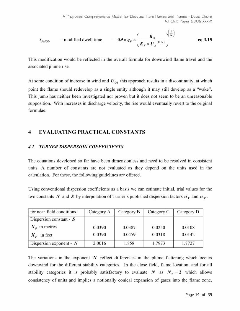
4 EVALUATING PRACTICAL CONSTANTS 4.1 TURNER DISPERSION COEFFICIENTS The equations developed so far have been dimensionless and need to be resolved in consistent units. A number of constants are not evaluated as they depend on the units used in the calculation. For these, the following guidelines are offered. Using conventional dispersion coefficients as a basis we can estimate initial, trial values for the two constants and by interpolation of Turner’s published dispersion factors and . N S Yσ Zσ

for near-field conditions Category A Category B Category C Category D Dispersion constant - S

FX in metres

FX in feet

0.0390 0.0390

0.0387 0.0459

0.0250 0.0318

0.0108 0.0142

Dispersion exponent - N 2.0016 1.858 1.7973 1.7727 The variations in the exponent reflect differences in the plume flattening which occurs downwind for the different stability categories. In the close field, flame location, and for all stability categories it is probably satisfactory to evaluate as which allows

consistency of units and implies a notionally conical expansion of gases into the flame zone.

N

N 2=TN

Page 14 of 39


This generates a small error in based on the published values for the various stability categories, which already vary significantly.

S

Φ

O

As needed, an alternative estimate for a corrected in any category may be made from the

formula XS

equation 4.1 )2()( −×= NX traveldownwindSS

Unfortunately, this correction requires an iterative aspect to the calculation procedure, but is easily accomplished with modern computing techniques. When establishing basic design conditions, it is probably satisfactory to anticipate the neutral stability Category “D”. When calculating , selections of a value for Cp depends to some extent on the particular

section of the plume under consideration. HF

• in the far field (plume strongly diluted by air) (specific heat of air) is appropriate. ACp

• within the flame, Cp (specific heat of discharge) is more

valid, even though this will transition to the specific heat of the flue gas as the flame proceeds.

O

It is also significant to bear in mind that wind speed varies with height and surface drag conditions. Conventionally, winds are specified at a given height above grade. At other elevations it is suggested to use a standard wind height correction such as that provided in ASCE-714 and noted below.

×= AAH H

HUU equation 4.2

where H = height in consideration = ref height for wind speed (most commonly 10 metres above grade) OH

= wind height exponent according to terrain [varies from 1/5 to 1/11 ] Φ

For consistency, the downwind distance to a modified value of should coincide with the mid

flame (or mid-plume) height used for the wind speed in the various prior formulae. XS

Page 15 of 39


4.2 COMPARISON WITH OTHER MODELS To examine the model, the prior formula for has been compared with available field data,

published data and the two, common flame models in API RP-521. The series of comparative graphs appended to this paper show flame shapes developed by this model (BUO), the Brzustowski model (BRZ) and the API “simple” (API) model. The conditions for each investigation are shown with each curve and all represent specific points plotted in RP-521 Figs 8 and 9.

FH∆

Very little data is provided with the API-521 flame length plot and a variety of assumptions have been made for each data point in order to facilitate a complete calculation. The variables needed for the models but not provided in RP-521 have been interpreted from the associated text and are all shown in the figures. Despite the need for assumptions, the new formulae appear to tie in fairly well to the available data for observed flames over a representative range of wind speeds. Similarities between the API simple curve and the BUO curves appear in moderate wind conditions but the models show differences in flame length at some wind speeds. The BRZ model does not readily concur with either the BOU model or the pattern of flames lengths of RP-521 Fig 8. These differences in the BRZ model highlight this author’s concerns about the overall suitability of the widely used BRZ model for flare design. 4.3 PRACTICAL FIELD OBSERVATIONS Practical readings of flame length taken in the field tend to be very subjective. Even if dimensions are accurately determined, the recorded conditions will rarely include a complete profile that includes all of the relevant stability conditions and included flows. 4.3.1 INCLUDED FLOWS AND GAS CHARACTERISTICS In most locations where flare flame length is of interest, and may be recorded, the gases being burned will probably be hydrocarbons which, if burned unassisted, will make smoke. Operation with an unnecessarily smoky flame during field readings is not a preferred mode of operation and it is quite possible that readings of flame length will be made on a clean flame, which is subjected to steam injection and is thus unrepresentative relative to the basic model. To make some accommodation for this factor, the additional materials in the flame (steam or air) need to be recorded and the adjusted value for C and CV allowed in the calculation of . L FK

Page 16 of 39


Shore15 provides an approach to assessment of C , for mixtures which include inert gases such

as steam, which may be beneficial in this matter. This will not include the influence of additional injection-based turbulence on the flame length. For a practical recording with a clean steam-injected flame, reduce the steam to the minimum tolerable to permit a “just clean” flame, before taking readings.

L

4.3.2 ESTIMATING THE STABILITY CONDITION Atmospheric stability is extremely variable and dependent on many environmental factors. For the BUO model, it also has significant influence on the flame shape. A nomograph (figure 6) has been prepared for the purpose of stability category estimation in the field, based on the descriptive texts of Turner and Briggs and the Solar radiation model of Bird and Hustrom16

5 THE PROCEDURE 5.1 CONVENTIONAL, VERTICAL FLARE DISCHARGES At the end-of-flame location , for conventional vertical flares, the model and calculation

procedure resolve to FX

a) determine the flow characteristics for the discharged gas [ ]ερ ,,,,, OLOF UCCVq

b) determine the physical characteristics of the flare [ ]OSS rDH ,,

c) determine the atmospheric reference conditions [ ] OAAAA HCpTUNSStability ,,,,,,,, Φρ

d) estimate or calculate corrected values of

Φ

×=

O

SAAS H

HUU for SH = stack height eq 4.2.1

Φ

×=

O

CAAC H

HUU for H = mid flame height eq 4.2.2 C

= downwind distance to mid flame CX

eq 4.1 )2( −×= NCX XSS

6.1=BK

3.2=MK

Page 17 of 39


X

S SK

××=

π21 eq 2.5

eq 2.4 LOF CCVK ××= ρ

×

×=

21

3ACF

SFF UK

Kqt eq 2.6

eq 2.7.1 FACF tUX ×=

2OO

FO rCV

q×××

=πρ

U eq 5.1

eq 3.12 )4.1(1 ASOO UUU ×−=

[ )5.1(1 ερπ

×−×

×××

=AAO

F TCpgF ] eq 3.7

221 OO

A

OM rU ××

=

ρρ

F eq 3.11

00 131

32

31

≤=××=

OF

AC

MMM UifX

U

FKH∆ eq 3.10

04.1

51

≤

×××=∆

O

ASSD U

UDH eq 3.13

( )

××

××=∆ 323

1

1 5.0 FAC

FFBF X

UqF

KH eq 3.1

= rise at flame end eq 5.2 DMFF HHHH ∆+∆+∆=∆ 1

e) determine the intermediate mid flame locus [ and iterate to convergence. ]CC XH ;

Throughout this analysis, the Zero wind condition is clearly an asymptote requiring an alternative treatment. This condition is not discussed in this paper and requires additional investigation. A limiting minimum wind speed of 1 fps (0.3 m/s) is suggested for calculations involving low wind speeds By substitution for U in the calculation of , the formula may be rearranged into the form O MF

""

667.0333.0

Bq

Aq

H FFF +=∆ eq 5.2.1

Page 18 of 39 where and are complex values including gas composition and velocity. "A "B


This solution shows a modest similarity to the common, logarithmic (straight line) solution of RP-521 fig 8

Flame length = 135

467.0F

FQ

L = ft eq 5.3

Heat release = Btu/h FF qQ ×= 3600

5.2 A THREE-DIMENSIONAL MODEL The need for a three-dimensional model is a main reason for the original development of this BUO model, and inclusion of momentum in the algorithm makes this possible. For the three dimension solution, the basic formula must be divided into the two main components a buoyant (thermal or density based) component which is always in the vertical direction ∆ 321 PPPPT HorHorHHZ ∆∆∆=∆=

a momentum component which is axial with the discharge

MΑ∆ replaces to indicate the vectored result of the axial displacement MH∆

The computation is performed most easily using time based formulae rather than distance based formulae and with vectored wind conditions as indicated below and illustrated in the attached figure 7. The following convention is suggested for representation of coordinates the angled discharge is at angle to the vertical tα the angled discharge always points towards the 0.0 degree plan reference angle angles are referenced from 0.0 degrees, clockwise in plan wind blows from orientation wα towards orientation degrees 180+= ww αβ

X = axial / horizontal direction/ distance + ve values towards 0 degrees Y = cross axis / transverse direction / distance + ve values right of 0 degrees Z = vertical direction / distance + ve values upward

cross discharge wind 22 ))cos()(cos())(sin( twwUU ASAO αββ ++×= eq 5.4 Page 19 of 39


cross axis wind eq 5.5 )sin( wUU ASAY β×=

axial direction horizontal wind eq 5.6 )cos( wUU ASAX β×=

turbulence adjusted discharge eq 5.7 ))sin((2 tUUU AXOO α×+=

downwash-corrected discharge U eq 5.8 )4.1(21 AOOO UU ×−=

the downwash correction is applied to the axial direction.

××

×××= 3

4

323

1

1 5.0 tUKK

FKH AFS

FFBF∆ equation 3.1.5

×

×=Α∆ 3

131

tUF

KAY

MMM equation 5.9

using constants and derived values as previously defined. Plotting the flame (or downwind plume) centerline locus becomes a simple solution of vectored values based on the defined X; Y; Z axes. All momentum-based travel is related to the discharge axis direction X

Vertical momentum travel = )cos( tZ MM α×Α∆=∆ equation 5.10

Horizontal momentum travel = )sin( tX MM α×Α∆=∆ equation 5.11

Total along-axis travel = equation 5.12 )( tUXX AXM ×+∆=∆

Cross-axis travel = equation 5.13 tUY AY ×=∆

Rise = =∆ equation 5.14 TM ZZZ ∆+∆

6 THE DOWNWIND PLUMES 6.1 THE OVERALL PLUME TRAJECTORY This model allows the standard plume formulae to be used in the down stream zone such that, during the plume rise section beyond the end of the flame, the actual rise is reduced by a fixed quantity equal to the rise difference between the end of the flame and the fully developed plume at the same downwind distance. From the prior analyses, it is clear that the end-of-flame thermal rise is one half (1/2) of the normal plume thermal rise at the flame end distance.

Page 20 of 39


The ability to generate a plume trajectory in the downwind near-field location of the flame, is not normally significant in plume calculations, when the overall objective is to determine ground level concentrations. In these cases, the theory relies on a plume which has already reached its final height and distributes, in a Gaussian manner, into the atmosphere. For these cases, the normal governing stability categories should be used, with appropriate selection of dispersion coefficients. The total plume rise to a horizontal condition is generally accepted to be limited by atmospheric turbulence. The height and distance limits for the maximum rise vary with stability condition. For stable and neutral conditions a range of down wind distances to a level plume is given by various authorities. Beychok17, and others provide a formula based on the Buoyancy parameter

. BF

4.0119 BFINAL FX ×= metres for units of given in mBF 4/s3 eq 6.1

This applies for values of m55≥BF 4.s-3, which corresponds to thermal sources in excess of

roughly 5.9 MW (or 20 million Btu/h), covering most flaring conditions. For a hot source is replaced by and for a flame source is replaced by . BF qFH × BF FF qF ×

For these distant field calculations, when final rise is limited as indicated, any height corrections due to the initial flame position will become insignificant to the final height of the plume. 6.2 CONCENTRATIONS IN THE DISTANT FIELD In the distant field, for calculations of ground level concentration, plume reflection at the ground is a factor and the dispersion formula is expressed as

WA

Tz

ZHz

ZHy

YUzy

×

+

×−

+

−

×−

×

×

−×

××××=

222

1 21exp

21exp

21exp

21

σσσσσπχ

equation 6.2 where = an eigenvalue for the specific property or pollutant to be investigated 1χ

= vertical elevation of plume centerline H Y = horizontal transverse distance from the plume centerline = vertical distance from the plume centerline Z

Page 21 of 39


yσ = horizontal dispersion coefficient for the relevant stability and distance

= vertical dispersion coefficient for the relevant stability and distance zσ T = time weighting multiplier (see below) W

Published horizontal and vertical dispersion coefficients are, generally, based on empirical results and are related to a specific sampling time. The limits set on ambient pollutant concentration are generally referred to as the REL (recommended exposure limit). These are also given as a TWA (time weighted average). When evaluating the probable downwind ground level concentration of pollutants from any source, including a flare, care must be taken to adjust the calculation in such a manner as to coordinate the time base of the dispersion coefficients with that of the REL. Turner gives an approximation of the relationship as

)17.0(

=

timeaveragingrequiredtcoefficienoftimeaveragingTW equation 6.3

Thus, dispersion values predicted using dispersion coefficients obtained from 10 minute sampling, are slightly higher than those appropriate for comparison with a typical OSHA TWA based on a 15 minute sample and should be reduced by the appropriate T W

6.3 NEAR-FIELD PLUME PROPERTIES When dealing with flares, often, a near-field estimate of plume trajectory is needed to assess whether a hot plume from the flame is likely to impact another piece of equipment, such as another flare, a tall distillation column or personnel access areas, and, if so, under what conditions and degree of severity. Application of the BUO model, with the height correction beyond the flame makes this possible. Because plume dilution occurs from the moment the flame commences, at the point of discharge, the standard dispersion coefficients should apply. As with the prior development of the flame dwell-time relationship, the important characteristics lie on the plume centerline, and the same simplifications should be practical for the down stream near-field, such that

AUzy ××××

=σσπ

χ2

11 equation 2.1.1

AX UXS ××××

= 21 21

πχ equation 2.1.2

where X = downwind distance Page 22 of 39


Most of the estimations needed in the near field represent a physical condition which may present an immediate hazard to personnel. For such cases, the subjective response of exposed personnel cannot, reasonably, be averaged over a 10 or 15 minute exposure time and a 3 second exposure would probably be a more appropriate sample time. Accordingly, using the prior time adjustment formula, a multiplier of T = 2.5 should be applied to the eigenvalue for these

conditions when possible personnel exposure is involved. W 1χ

Applying this technique to the flame we find that

Plume Temperature (above ambient) AA

FW Cp

qT

ρεχ

×××−××= )5.11(1 eq 6.4.1

With substitution of the prior relationship for downwind distance at the flame end, it can easily be seen that this yields a flame end temperature that corresponds to the flame temperature at the lean limit, without the application of the factor T . However, this is such an obviously

dangerous location and high temperature that downwind investigations will not normally be performed. Further down wind the 2.5 multiplier introduced by T can be seen to represent a

realistic factor of safety. Additional analysis yields a rule of thumb that plume temperatures may be intolerable for a downwind distance of roughly 20 flame lengths.

W

W

Unburned gas concentration

−

×××=100

1001

ηχ OW wT [M.L-3] eq 6.4.2

( ) 000,000,11001 ×−×××= ηρ

χO

OW

wT [ ppm ] eq 6.4.3

where = pollutant output rate into the flame Ow

η = destruction efficiency in flame

Flue gas concentration Down wind flue gas concentration depends on the rate of flue gas production, which in turn depends on the original gas composition. Where this can be determined, and a flow rate calculated, downwind concentrations are calculated directly from the eigenvalue [M.LFW wT ××= 1χ -3] eq 6.4.4

where output of Flue Gas = eq 6.5 Fw OF wR ×=

Page 23 of 39


= Mass Ratio of Flue gas to flammable component FR

If the gas composition is not known in sufficient detail to determine a value for RF, a reasonably accurate estimate may be made by “rule of thumb”, based on the heat release. It is usually possible to obtain a first order estimate of flue gas rate (+/- 20%) from

1R

FF K

qw = equation 6.6

applying a representative flue gas MW = 28 downwind,

this yields a concentration of flue gas 1

1R

FW K

qT ××≈ χ [M.L-3] equation 6.4.5

where = 1200 Btu/lb ~ 667 kcal/kg 1RK

or a Vol Concentration of Flue Gas % vol equation 6.7 21 RFWF KqTV ×××≈ χ

where = 1.13 % / Btu ~ 0.285 % / kcal 2RK

Oxygen concentration is determined directly from the flue gas concentration such that % vol equation 6.8 )100(21.0 FOX VV −×=

A breathable concentration needs to be greater than 19.5 % Oxygen. Substitution of previous results suggests that a minimum of 5 clear flame lengths is necessary to avoid oxygen deficit. Given the, earlier, similar finding that 20 clear flame lengths may be necessary to avoid high flue temperatures, it seems elevated temperature can serve as an adequate warning to personnel to escape from an engulfing plume of flue gas. Of course, this must be tempered by knowledge of any other, potentially harmful constituents of the plume. For a non-vertical tip, the locus of the near field, downwind plume is offset from the wind line through the tip discharge according to the offset formulae previously outlined for the three-dimensional flame itself. As with a vertical tip, the vertical thermal rise can be calculated from the normal plume rise formulae with the appropriate adjustment for the flame end rise.

Page 24 of 39


6.4 RADIANT CENTER Although the main purpose of this model is to define conditions other than the radiant output of the flame, the nature of the model is such that it may posibly be used for Radiant predictions in the same manner as the API and BRZ models previously discussed. At this time, no investigations have been performed which suggest a departure from the common, point source spherical model., although preliminary review of photographic evidence strongly indicates a common flame shape, predictable using equation 6.9. Based on the flame residence time formula of this paper, as the gas burns within the flame, and the heat release develops to fraction , the downwind travel relationship can be adjusted

accordingly.

j

AF

J UKKSqFjX×

××= equation 2.7.2

One possible measure of the center of the flame occurs when 50% of the gas has been consumed, at such that or 70% of the downwind flame length. or as

required may be calculated using the previous formulae with appropriate substitution of .

5.0=j FC XX ×≈ 7.0 CH∆ CZ∆

CX

An alternative approach to radiant center may be derived from the same distribution pattern used for the initial development of the flame model which develops as a relationship for

flame radius parameter { }22 2ln2 RRR σπχσ ×××××−= equation 6.9

where equation 6.10 22 XS XR ×=σ

using previously defined parameters. Plume radius calculated from this formula needs an additional multiplier to incorporate the volume expansion due to high temperature, in order to generate a meaningful flame shape. This approach, when integrated, together with photographic evidence, suggests a “pseudo-spherical” center at roughly 60% of the flame length and is probably the most realistic practical selection. More formula development is required, however, before the appropriate flame emissivity (or radiated fraction) can be adequately related to this flame shape or the equivalent radiant sphere.

Page 25 of 39


7 FLAME EFFICIENCY An interesting aspect of the flame “dwell time” model is a possible tie-in to flame efficiency predictions.

Johnson et.al18 suggested that there exists a relationship of 31OA UU which allows prediction of

flame inefficiency. Their text suggests that efficiency improves with heat content of the flammable material but is independent of total heat release. However, an alternative treatment may yield an alternative conclusion. Rearranging the limited data published in the Johnson paper allows all the curves to be redrafted, with good accuracy, in the form

( )

××=−

23

3121 exp100O

AC U

UKKη equation 7.1

Interpolated data from the Johnson paper is compared with this formula in the enclosed graph figure 8. This, can be expressed using a re-arrangement of the prior formula for , such that Ft

3

22

2 A

O

L

OF U

UCS

rt ×

××= equation 2.6.2

or LO

F

A

O CSrt

UU

×××= 23 equation 2.6.3

leading to

−

×=−F

TC t

KK exp100 1η equation 7.2

which is the well known form for growth and decay relationships, in which the effective basis is the theoretical residence time of the flame reaction given by the BUO formula. The values for

and shown here as constants, will undoubtedly prove to be a functions of the other

physical characteristics of the system and are clearly targets for further research. 1K TK

Factors already in evidence, which may influence the overall equation include the jet size, the lean limit concentration of the fuel mixture and the stability parameter . For the small-scale Johnson work in a wind tunnel the neutral case is suggested.

S

Page 26 of 39


Other factors may include a measure of the initial rate of conversion at the commencement of the flame (t = 0), or the superficial rate of regression, which would suggest an involvement of the component reactivity as discussed previously. This possible link with efficiency is a very significant finding as it predicts high conversion efficiencies for those conditions which would exist during field-testing, and during which high conversion efficiencies have been practically determined. It also leads to a conclusion of high conversion efficiency for the emergency design cases, which are the bases of most elevated flare designs. However, it raises the possibility of very poor efficiencies for the majority of industrial flares when operating on low-load, which is the common, day-to-day condition. The potential significance of this possible relationship mandates more testing before the formula can be applied as anything other than an estimate.

8 CONCLUSION The author recognizes that this has been, primarily, a theoretical, mathematical analysis and that many of the ideas introduced may conflict with current calculation procedures and furthermore, that in some ways, the model may raise more questions than it answers. However, in addition to the mathematical arguments expounded in the forgoing, the analyses are also based on the author’s personal observations and experience over many years of dealing with combustion and flares. The overall aim has been to produce generally more useful algorithms than those in common use at this time. As a result of this approach it has been possible to bring together many separate elements of flare flame and plume analysis. This complete model generates information which may be used, together with other standard methods, to estimate - flame positions for any direction of discharge or wind - flare flame size and “center” location for radiant heat calculations - flame centerline and plume locus for near field impact studies - plume centerline locus for far field pollutant concentration studies - flame residence time for estimations of component destruction efficiency - flame residence/wind relationships for estimations of component combustion efficiency - the specific disruptive effects of down-wash in the lee of the flare tip.

Page 27 of 39

As far as practical, the results of this analysis have been cross referenced against field results but others are strongly encouraged to generate field data or specific research analyses for additional


cross references, in all areas of the extended models covered by this paper. If desired, such data may be submitted to the author for this purpose.

Page 28 of 39


CAUTION The reader is cautioned that calculations for downwind pollutant REL may be subject to regulatory approval and that Regulatory Authorities may require calculations to be performed according to a specific protocol. This treatise is not intended to supplant those methods for distant field calculations but simply to highlight the effects in the local plume and provide a means of estimating often-overlooked, near-field values.

ACKNOWLEDGEMENTS The author wishes to thank the Management of Flaregas Corporation for facilitating the preparation and presentation of this paper, and the AIChE Session Chairman for his assistance with editing and formatting the final presentation. The AUTHOR David SHORE has made a number of presentations on Flaring to A.I.Ch.E,, other major Institutions and Corporate Bodies. He has been involved with Combustion and Flare Design since 1965 and is employed as the Chief Engineer of Flaregas Corporation in New York, U.S.A. Mr. Shore is a frequent contributor to Engineering Fora, and maintains a web site dedicated to consultancy on technical issues of Combustion and Flaring.

Page 29 of 39


FIGURES

Page 30 of 39


Figure 1 - Calculated Flame Pattern / Algerian gas Well

Derived and Estimated Values for Flame Position Calculations - Ref API-521 Fig 8

Flow Rate 2,000,000 lb/h Wind Speed 18 fps RP-521 Length 600 ft Mol Weight 23.9 Solar Contrib 370 Btu/sq.ft_h BRZ Length 268 ft Temperature 150 deg F Stability C BRZ Rise 238 ft Calorific Value 20160 Btu/lb Flare Height 25 ft BRZ Travel 66 ft LEL 4 % API Length 664 ft Total Heat 4.0E+10 Btu/h BUO Rise 576 ft API Rise 444 ft Flare Dia 42“ BUO Travel 378 ft API Travel 383 ft

Page 31 of 39


Figure 2 - Calculated flame Pattern / Hydrogen Flare


Flow Rate 280,000 lb/h Wind Speed 40 fps RP-521 Length 430 ft Mol Weight 2 Solar Contrib 250 Btu/sq.ft_h BRZ Length 453 ft Temperature 200 deg F Stability D BRZ Rise 165 ft Calorific Value 51625 Btu/lb Flare Height 200 ft BRZ Travel 381 ft LEL 4 % API Length 412 ft Total Heat 1.45E+10 Btu/h BUO Rise 218 ft API Rise 314 ft Flare Dia 30“ BUO Travel 564 ft API Travel 192 ft

Page 32 of 39


Figure 3..- Calculated flame Pattern / Catalytic Reformer Effluent


Flow Rate 200,000 lb/h Wind Speed 20 fps RP-521 Length 210 ft Mol Weight 59.4 Solar Contrib 250 Btu/sq.ft_h BRZ Length 138 ft Temperature 350 deg F Stability D BRZ Rise 59 ft Calorific Value 19620 Btu/lb Flare Height 150 ft BRZ Travel 110 ft LEL 1.7 % API Length 224 ft Total Heat 3.9E+9 Btu/h BUO Rise 127 ft API Rise 91 ft Flare Dia 24“ BUO Travel 201 ft API Travel 180 ft

Page 33 of 39


Figure 4 - Calculated flame pattern / Catalytic Reformer Recycle gas



Page 34 of 39


Figure 5 - Calculated Flame pattern / dehydrogenation unit



Page 35 of 39


Figure 6 - Nomograph to Estimate Solar Conditions and Stability Categories

Page 36 of 39


Figure 7 - Directional Conventions for Three Dimensional Flame Model

Page 37 of 39


Figure 8 - Combustion Inefficiency for small jet in Wind Tunnel

Page 38 of 39


BIBLIOGRAPHY

1 Recommended Practice RP-521; Guide for Pressure-Relieving and Depressuring Systems; American Petroleum Institute, Washington. D.C.

2 Brzustowski, T.A., & Sommer, E.C. Jr.; “Predicting Radiant Heating from Flares”; Proceedings – Division of Refining, Volume 53, pp 865-893; American Petroleum Institute, Washington. D.C; 1973.

3 Majeski, A.J., Wilson, D.J.& Kostiuk, L.W.; “Local maximum Flame Lengths of Flares in a Crosswind”; Combustion Inst (Canadian section); May 1999.

4 Hottel. V.O., & Luce, R.G.; “Burning in Laminar and Turbulent Fuel Jets”; Fourth Symp (intl) on Combustion; the Combustion Institute; 1953.

5 Zukoski, E.E.; “Scaling Flame lengths of Large Diffusion Flames”; National Institute of Standards and Technology, Annual Conference on Fire Research; pp 39-40; 1996.

6 Gogolek, P.E.G. & Hayden, A.C.S.; “Wind Turbulence and Elevated Flare Flames”, Presentation to the American Flame Research Committee, 2004.

7 Pasquill, F.; “The Estimation of the Dispersion of wind borne material”; Meteorol Mag. 90, 1063, 33-49, 1961.

8 Gifford, F.A.; Atmospheric Dispersion calculations using the generalized Gaussian Plume model”, Nuclear safety, 2, 2, 56-59, 67-68, 1962

9 Turner. D.B.; “Workbook of Atmospheric Dispersion Estimates”; U.S. Dept of Health, Education & Welfare, 1967

10 Pohl. J.H., Payne. R., and Lee.J; “Evaluation of the Efficiency of Industrial Flares”; U.S. Environmental Protection Agency; EPA-600 / 2-84-095

11 Briggs. G.A.; “Plume Rise”; U.S. Atomic Energy Commision, 1969

12 Simiu. E. and Scanlon R.H.; “Wind Effects on Structures”; Wiley-Interscience Publications, 1978

13 Von Karman, T.; “Über den Mechanismus des Widerstandes den ein bewegter Körper in einer Flüssigkeit efährt”; Nachrichten der Könglichen Gesellschaft der Wissenschaften, 1911.

14 ASCE-7-98; “Minimum Design Loads for Buildings and Structures”; A.S.C.E (publ 1998) [Issues of ASCE-7 which post-date 1998 are available with more complex height exponents but which are more applicable to

structural design. Appropriate terrain characteristics should be interpreted per the code parameters.].

15 Shore.D; “Making the Flare Safe”; A.I.Ch.E, Proceedings of 30th Loss Prevention Symposium, Paper 12d. 1996.

16 Bird. R.E. and Hulstrom. R.L.; "A Simplified Clear Sky model for Direct and Diffuse Insolation on Horizontal Surfaces" . Solar Energy Research Institute, Golden, Co; SERI Technical Report SERI/TR-642-761, Feb 1991

17 Beychok, M.R.; "Fundamentals Of Stack Gas Dispersion", published by the author, fourth edition, 2005.

18 Johnson. M.R., Zastavniul. O., Wilson. D.J. and Kostiuk. L.W.; “The Combustion Efficiency of jet Diffusion Flames in Cross-flow”; Presentation to The Combustion Institute, Washington D.C.; March 15-17, 1999.

Page 39 of 39

Documents

A PROPOSED COMPREHENSIVE MODEL FOR Proposed Comprehensive Model for Elevated Flare Flames and Plumes - David Shore A.I.Ch.E Paper 2006 XXX-X A PROPOSED COMPREHENSIVE MODEL FOR ELEVATED