Syracuse University Syracuse University

SURFACE SURFACE

Electrical Engineering and Computer Science - Technical Reports College of Engineering and Computer Science

4-1990

A Proof for a QuickHull Algorithm A Proof for a QuickHull Algorithm

Jonathan Scott Greenfield, Syracuse University

Follow this and additional works at: https://surface.syr.edu/eecs_techreports

Part of the Computer Sciences Commons

Recommended Citation Recommended Citation Greenfield,, Jonathan Scott, "A Proof for a QuickHull Algorithm" (1990). Electrical Engineering and Computer Science - Technical Reports. 65. https://surface.syr.edu/eecs_techreports/65

This Report is brought to you for free and open access by the College of Engineering and Computer Science at SURFACE. It has been accepted for inclusion in Electrical Engineering and Computer Science - Technical Reports by an authorized administrator of SURFACE. For more information, please contact surface@syr.edu.

SU-CIS-90-03

A Proof for a QuickHull Algorithm

Johnathan Greenfield

April 1990

School of Computer and Information ScienceSuite 4-116

Center for Science and TechnologySyracuse, New York 13244-4100

(315) 443-2368

A Proof for a QuickHul1 Algorithm

Jonathan Greenfield

School of Computer and Information ScienceSyracuse University

Syracuse, New York 13244

April 1990

Abstract: The planar convex hull problem is fundamental to computational geometry and has manyapplications, including pattern recognition and image processing. QuickHull is a simple planar convex hullalgorithm analogous to Hoare's QuickSort [1]. This paper presents a pedagogical description and analysisof a QuickHull algorithm, along with a fonna! proof of correcbless.

Keywords: complexity analysis, computational geometry, convex hull, correctness proof, divide-and­conquer, prune-and-search, QuickHull.

1. Introduction

Many algorithms have been proposed in order to solve the planar convex hullproblem [2]. The algorithms are varied, but generally they have time complexities of eitherO(n log n) (such as Graham's Scan [3]) or O(mn) (such as Jarvis' March (the package­wrapping method) [4]), where n is the number of points and m is the number of hullvertices [2]. Divide-and-conquer algorithms have been proposed [5,6] includingalgorithms with linear expected running time [6].

This paper describes a simple divide-and-conquer, prune-and-search algorithmfor finding the convex hull of a finite number of planar points. Although our version ofthis algorithm was developed independently, [7,8,9] proposed similar versions of thisalgorithm previously (later termed QuickHull algorithms by [10]). In contrast to theQuickHull descriptions of [7,8,9,10], we present a proof of correctness for our algorithm.The proof offers some insight into the difficulty in generalizing this algorithm for oon­planar convex hull problems.

The algorithm has a worst-case time complexity of 0(n2), but an expected timecomplexity of 0(0 log n), when all points are hull vertices. Furthermore, when the numberof hull vertices is small compared to the number of points (in an asymptotic sense, as is thecase for many distributions [7,11]), the algorithm has an expected time complexity of O(n).

2. Informal problem definition

The convex hull problem is one of the common computational geometry problemsand has many applications, including pattern recognition and image processing. We candevelop an intuitive understanding of the problem by [rrst considering the planar convexhull problem (for a finite set of points).

Consider a finite set of points in two dimensions (fig. la). Suppose that each ofthe points is a nail that has been hammered into a piece of wood. We stretch a rubber bandso that it surrounds all of the nails (fig. Ib), and then release the rubber band, allowing it tocontract around the nails (fig. Ic).

I

•

8.)

••

•

•

••

•

•

b) c)

Figure 1: Intuitively constructing the convex hull o/points in the plane

Now, we can easily visualize the convex hull of the set. It is precisely the areaenclosed by the rubber band (fig. Ic). Note that the rubber band fonns the boundary of theconvex hull, and that the boundary has the shape of a convex polygon. Further note thatsome of the nails touch the rubber band and form vertices of the bounding polygon. Othersdo not, and are inside of the rubber band.

Finding the convex hull is precisely the problem of identifying these vertices (inclockwise or counter-clockwise order). We may note that, in general, the convex hull is aninfmite set, which is described by a fmite number of points: the vertices of the boundingpolygon.

This informal definition of the convex hull may be generalized for points inarbitrary dimensions. It is, however, not as easy to envision as the two-dimensional case.

3. Formal problem definition

A set, S, of points in an Euclidean space is said to be convex if and only if for allpairs of points, p and q, in S, every point on the line segment connecting p and q iscontained in S.

The convex hull of a set, S, is defmed to be the smallest convex set that containsS. A convex hull is normally described by its boundary. The boundary of the convex hullof a set, S, is denoted CH(S).

A common convex hull application requires fmding the convex hull of a finite setof points lying in the plane. For this problem, CH(S) consists of a convex polygon. Wedescribe CH(S) by an ordered set of vertices for the convex polygon which fonns theboundary of the hull.

Note that there are both primary and secondary vertices for the polygon. Aprimary vertex of a polygon is a vertex that joins two sides of the polygon. Any point onthe polygon which is not a primary vertex is a secondary vertex. Clearly, all primaryvertices are necessary to define the polygon. Secondary vertices mayor may not beincluded in the definition of the polygon, without changing the polygon.

In general, we are not particularly concerned with the inclusion of somesecondary vertices in our definition of CH(S) since there is a very quick and simple

2

method for removing them. Our algorithm, in its simplest form, does not distinguishbetween primary and secondary vertices. However, we shall present the algorithm in aform which produces only primary vertices, since the algorithm is not significantlychanged, but the corresponding proof of the algorithm is considerably simplified.

4. The algorithm

The algorithm is based on the idea of triangular expansion. We consider twoprimary vertices, p and q (fig. 2a). The two vertices define a line segment, pq (fig. 2b).This line segment forms the baseline of some triangle. We define the right and left sides ofa baseline, pq, to be relative to baseline pq viewed vertically, with point p above point q.For simplicity, we assume that all points under consideration lie to the right of pq. Weselect a third primary vertex, r, to the right of the baseline, forming triangle pqr (fig. 2c).

We have now generated two new line segments, pr and rq. We repeat the aboveprocess, recursively, by considering the two segments as baselines (separately). This isthe divide step. When we consider baseline pr, we select a primary vertex, S, to the rightof the baseline. This forms triangle prs (fig. 2d). We end the recursive repetitionwhenever we discover a baseline for which no point lies to the right of the baseline (fig.2e).

I

p

q

c)

•I

•

•

a) b)

P e p• •• •

• •• •• •• • ••• •• •

• •• •• •

q e q

d) e)

p

q

Figure 2: Graphic depiction oftriangular expansion

3

Note that this process may be viewed as the (triangular) expansion of anapproximate bounding polygon for the convex hull. Our initial approximation consists ofthe two-sided polygon defined by the two primary vertices initially selected (fig. 2b). Ateach step, we include one additional primary vertex into our approximate set of vertices,expanding the approximate bounding polygon (fig. 2c-e). When all primary vertices havebeen included, the approximate bounding polygon is the actual bounding polygon for theconvex hull (fig. 2e).

Since the approximate bounding polygon always defines a subset of the convexhull, points internal to the approximate bounding polygon are internal to CH(S). We may,therefore, ignore any points found to be internal to the approximate bound polygon. Notethat we have done this, implicitly, via our process of selecting primary vertices only fromthe set of points to the right of the baseline under consideration. This is the prune-and­search element of the algorithm.

In general, it is difficult to select our two initial primary vertices so that all of thepoints under consideration lie to the right of the initial baseline. Rather, it is easier for us toselect two convenient primary vertices, such as the vertices with maximum and minimumy-coordinates. As a result, we initially divide the problem into two subproblems: onecorresponding to baseline pq, along with the points to its right, and one corresponding tobaseline qp, along with the points to its right (which are to the left of baseline pq -- fig.3).

•

•

••

•

q

p

•

•---

•

•

••

•

q

p

+

q

p

•

•

Figure 3: Dividing the initial problem into two subproblems

We now need only consider the primary vertex selection process. For thispurpose, we introduce a formal defmition of the algorithm.

Consider finding the convex hull of a fmite set of points, S, where every point inS lies in the plane and is described by an x-coordinate and a y-coordinate. We assume thatthere are at least two distinct points in S. We defme algorithm Hull as follows:

InputSet(S);Select(p,q,S);Split(p,q,S,R,L);OutputPoint(p);QuickHull(p,q,R);OutputPoint(q);QuickHull(q,p,L)

4

Select (p, q, S) selects two points of S which are primary vertices of CH(S) (fig. 4).It is convenient to choose the points with the maximum and minimum y-coordinates (usingx-coordinate values to break ties).

s:

• e P• •

• •• •

• • • •• • •

• •• •

e •q

Figure 4: Selecting two initial primary vertices: Select(p,q,S)

Split (Pr q, S, R, L) splits S into three sets, R, L, and 0 (fig. 5). These sets containthe points of S to the right of baseline pq, to the left of baseline pq, and on baseline pq,respectively. (Note that the set 0 is not required by the algorithm. As such, points in theset 0 are discarded.)

s:

Figure 5: Splitting the data points into disjoint sets: Split(p,q,S,R,L)

5

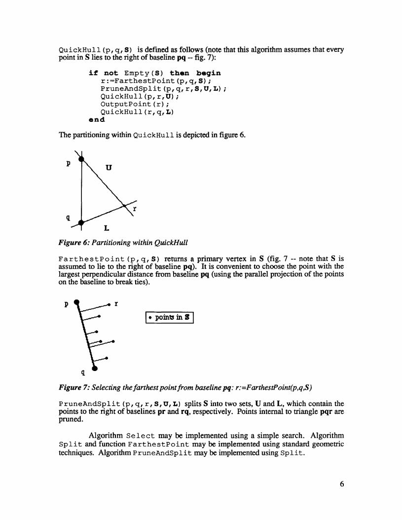
QuickHull (p, q, S) is dermed as follows (note that this algorithm assumes that everypoint in S lies to the right of baseline pq -- fig. 7):

i:f not Empty (8) then beginr:=FarthestPoint(p,q,S);PruneAndSplit(p,q,r,S,O,L);QuickHull(p,r,U);OutputPoint(r);QuickHull(r,q,L)

end

The partitioning within QuickHull is depicted in figure 6.

p u

q

Figure 6: Partitioning within QuickHull

FarthestPoint (p, q, S) returns a primary vertex in S (fig. 7 -- note that S isassumed to lie to the right of baseline pq). It is convenient to choose the point with thelargest perpendicular distance from baseline pq (using the parallel projection of the pointson the baseline to break: ties).

p r

I- pain" in S I

Figure 7: Selecting thefanhest point/rom baseline pq: r:=FarthestPoint(p,q,S)

PruneAndSplit (p, q, r, s, U, L) splits S into two sets, U and L, which contain thepoints to the right of baselines pr and rq, respectively. Points internal to triangle pqr arepruned.

Algorithm Select may be implemented using a simple search. AlgorithmSplit and function FarthestPoint may be implemented using standard geometrictechniques. Algorithm PruneAndSplit may be implemented using Split.

6

Our algorithm Hu11 is now complete. The primary vertices of CH(S) are outputin proper order. Listing 1 (at the end of this paper) is a Pascal implementation of thecomplete Hull algorithm.

s. Correctness proof

We shall prove that our algorithm correctly identifies the convex hull in threeparts. First, we shall prove that our algorithm outputs only primary vertices of CH(S).Next, we shall prove that all primary vertices of CH(S) are output. And finally, we shallprove that the vertices are output in proper order.

Theorem 1: Algorithm Hull outputs only primary vertices of CH(S).

Proof:

Defme a supporting line of a set S to be a straight line that has at least one point in commonwith S and all vertices of S lying on the same side (inclusive) of the line [2]. Clearly, anypoint of S which lies on a supporting line of S is in CH(S).

Consider a supporting line, L, of S (fig. 8). Assume that n points in S lie on L.Clearly, the two (end) points that fonn the longest line segment along L are primaryvertices [10].

s:L

•

• •• •• • • •

•

Figure 8: A set, 5, and supporting line, L

Algorithm Hull outputs points p and q. The points p and q are chosen to havethe minimum and maximum y-coordinates. Therefore, each point defmes a horizontal linethrough the point which constitutes a supporting line of S. Therefore, both points are inCH(S). Furthermore, we use the x-coordinates to insure that both points are endpoints.Therefore, both points are primary vertices.

Algorithm QuickHull (p, q, R) may be shown to output only primary verticesin eH(S) by strong mathematical induction on the cardinality of R. We shall use thefollowing invariant for algorithm QuickHull:

Invariant QH: 1) p and q are primary vertices in Cn(S)2) R is a subset of S and lies to the right of baseline pq3) the set S - R lies to the left of baseline pq

7

Clearly, algorithm Hull establishes this invariant for both of its calls to QuickHull.

Basis step: If IRI = 0 then QuickHull outputs no vertices. This vacuously establishes theconclusion.

Inductive step: Assume the conclusion for 0 S; IRI s: n. Consider the case of IRI = n+l.Assume the invariant, QH. QuickHull selects and outputs a point, r, in R, furthest frombaseline pq (fig. 9). Let L be a line drawn parallel to the baseline and through point r.Clearly, L is a supporting line of R, where R lies to the left of L. Furthermore, thebaseline lies to the left of L, and S - R lies to the left of the baseline. Therefore, S lies tothe left of L, and L is a supporting line of S. Therefore, point r is in C H (S).Furthermore, we choose point r to be an endpoint. Therefore, point r is a primary vertex ofCH(S).

•

•

L

p•

• • I

• •• • •• ••

• • ••• ••q

• points in R• points in S - R

Figure 9: Selection o/primary vertex r

IR - {r}1 = n. Therefore, no matter how we partition the set, our recursive calls toQuickHull will consider sets with cardinality S; n. We, therefore, need only prove thatour recursive calls to QuickHull maintain the invariant QR

Let us refer to the two recursive calls to QuickHull, for the baselines pr and rq, as case1 and case 2, respectively (fig. 10).

p

r

q

Figure 10: Constructing recursive calls to QuickHull

The maintenance of part 1) of QH is trivial for both cases.

8

The maintenance of part 2) of QH is trivial by our pruning-and-splitting algorithm. (Notethat no point of R - {r) lies both to the right of baseline pr and to the right of baseline rq.This is a result of the fact that L is a supporting line of R.)

We shall prove that part 3) of QH is maintained for case 1. The proof for case 2 isanalogous and trivially follows from the proof for case 1.

Consider case 1 (fig. 11). We call QuickHull (p I r, U). That R - U lies to the left ofbaseline pr is trivial by our splitting algorithm. We, therefore, need only show that S - Rlies to the left of the baseline. We show this by contradiction.

I!

S-RR-U

q

Figure 11: Partitioning ofsets for case 1

Assume there is some point, e, in S - R that is not to the left of the baseline. This point isin set E of fig. 11. However, if e is in E then, clearly, point p is not a primary vertex (fig.12). This is a contradiction of part 1) of QH. Therefore, set E is empty, and S - R lies tothe left of baseline pr.

Figure 12: Considering a point, e, in E

9

Therefore, invariant QH is maintained, and all points output are primary vertices ofCH(S).

Theorem 2: Algorithm Hull outputs all primary vertices of CH(S).

Proof:

The proof is trivial using strong mathematical induction. We provide an outline for theproof.

Clearly, algorithm Hull and every call to QuickHull results in the removal ofa finite number of points (~) from the original set, S. Furthermore, there are only twoways of removing points: recognizing that a point is a primary vertex, in which case thepoint is output, and recognizing that a point is internal to the polygon formed by thecurrently known primary vertices, in which case the point is not a primary vertex. Therecursive calls to QuickHull end only when all points of S have been removed. Since allprimary vertices are output when removed, the algorithm can not terminate until all primaryvertices have been output

Furthermore, it is clear that the algorithm terminates since we may bound thenumber of recursive calls to QuickHull from QuickHull (p, q, R) by 2*IRI.Therefore, algorithm Hull outputs all primary vertices of CH(S).

Theorem 3: Algorithm Hull outputs the primary vertices of CH(S) in proper order.

Proof·

The proof is trivial by strong mathematical induction.

Consider a call QuickHull (p, q, R). We use strong mathematical inductionon the cardinality of R to show that QuickHull outputs the primary vertices in R inproper order.

Basis step: If IRt = 0 then no points are output and the conclusion is vacuously established.

Inductive step: Assume the conclusion for 0 ~ IRI ~ n. Consider the case of IRI = n+1. Asshown previously, a primary vertex, r, is selected, and both recursive calls to QuickHullinvolve sets with cardinality ~ n. Therefore, both the upper and lower calls (cases 1 and 2,respectively) result in outputting the two subsets of primary vertices in proper order.Clearly, primary vertex r must be output between the two calls in order to maintain properorder. Therefore, algorithm QuickHull outputs the primary vertices in proper order.

Furthermore, given this proper ordering of output vertices by algorithmQuickHull, it is clear that algorithm Hull will result in a proper ordering of outputvertices.

We, thereby, complete our proof of algorithm Hull.

10

6. Time complexity

In general, the time complexity of geometric algorithms is difficult to analyze ascharacterization of the data is not simple [11]. We offer the following simple analysis ofthe time complexity of this algorithm. We consider data consisting of n points, m of whichare actually primary vertices. Note that the searching and splitting operations of algorithmHull will always have a time complexity of O(n).

Case 1: (almostl every point a primaIy vertex:

This is the case where m is O(n). Clearly, this is the worst case for any convexhull algorithm, since all primary vertices must be output. We consider two subcases: theworst subcase, in which the points are distributed such that our partitioning of points(almost) always generates one empty call to QuickHull (an empty call is one in which nopoints lie to the right of the given baseline), and the best (expected) subcase, in which thepartitioning of points is (reasonably) even.

The worst subcase:

The worst subcase for case 1 is clearly the worst possible case for the algorithm.Clearly, we require O(n) calls to Qui c k Hull, each of which requires an O(n)computation, on average. We, therefore, have a worst case time complexity of 0(n2). Asample point distribution which achieves the worst-case time complexity is shown in fig.13.

Figure 13: A worst-case point distribution

The best (expected) subcase:

Here, we assume that our partitioning of the data within Qui c k Hull is(reasonably) even. Clearly, by the divide-and-conquer nature of the algorithm, we have atime complexity of O(n log n) for this case.

Case 2: (reasonably) unifonnly distributed points:

This is the (expected) m «n case. For this case we also have two subcases: aworst subcase, in which the primary vertices are distributed such that our partitioning of

11

points (almost) always generates one empty call, and the best (expected) subcase, in whichthe partitioning of points is (reasonably) even.

The worst subcase:

We clearly have O(m) calls to QuickHull, each of which requires (no morethan) an O(n) computation. We, therefore, have a time complexity of O(mn) for this case.

The best (expected) subcase:

For our analysis, we assume that most of the points internal to the boundary ofthe convex hull are removed from the computation in the very early stages algorithm. Thisseems reasonable for problems involving reasonably uniform distributions of points sincethe early stages of the algorithm account for the vast majority of the area from whichinternal points are pruned. We, therefore, assume that after the early stages, O(m) pointsremain to be considered.

After the early stages, we clearly have a time complexity of O(m log m) by thedivide-and-conquer nature of the algorithm. The early stages have a time complexity ofO(n). The overall time complexity is, therefore, O(n + m log m). If we assume that m isO(n1/3) (which is a reasonable upper bound for circular distributions, rectangulardistributions, and several other distributions [11] as well as for a number of non-uniformdistributions [7]), then we have a time complexity of O(n) for the algorithm.

Performance measurements:

In order to provide some verification of our expected-case time complexityresults, we performed some simple perfonnance experiments. We applied the algorithm(using the implementation of listing 1) to randomly generated sets of points, uniformlydistributed in both rectangular and circular configurations. For each data set size, werandomly generated five rectangular distributions and five circular distributions. Tables 1and 2 show the average number of operations performed by the algorithm for therectangular and circular distributions, respectively. Graph 1 shows the average number ofoperations versus the total number of points, plotted for both distributions.

Table 1: Average number ofoperations for uniform rectangular distributions

Table 2: Average number ofoperations for uniform circular distributions

These performance figures show an essentially linear increase in the number ofoperations performed as the number of data points is increased. The figures, therefore,tend to support our expected-case time complexity analysis.

12

63000

100009000

Rectangular distribution

O~---------------------------------'o 1000 2000 3000 4000 5000 6000 7000 8000

Circular distribution

Average number of operations

7000

56000

14000

21000

28000

35000

42000

49000

Total number of points

Graph 1: Average number ofoperations for the two distributions

7. Space complexity

Consider a convex hull problem consisting of n data points, m of which areactually hull vertices. Every non-empty call to QuickHull (p, q, R) results in apartitioning of R into three sets (one for each of the two recursive calls to QuickHull, aswell as one for the internal points), without duplication. Furthennore, since O(m) calls arerequired for the complete algorithm, no more than O(m) activation records will exist at anyone time. Therefore, the activation records collectively contain no more than O(n) pieces ofinformation, and an efficient implementation of the algorithm will require only O(n)memory.

Note that the implementation of listing 1 depends upon the automatic reclamationand re-use of storage space (released by the removal of points from a set) in order toachieve the above space complexity. This is a result of the abstraction of the set data type.If necessary, the data type abstraction may be removed in order to allow manualreclamation and re-use of storage space.

13

8. Special cases

There are three special cases for the convex hull problem. They correspond tofinding the convex hull of an empty set, a non-empty zero-dimensional set, and an one­dimensional set. We have already seen that our algorithm works for the special case of anone-dimensional set It is trivial to include provisions for the other two special cases in ouralgorithm. Note also that our algorithm does not depend on distinctness of points in thedata set, S (as long as there are at least two distinct points).

9. Conclusion

We have presented a proof of correctness for a simple QuickHull algorithm. Thealgorithm has a worst case time complexity of 0(n2), but an expected time complexity ofO(n). The algorithm requires only O(n) memory.

We had originally hoped that this algorithm would generalize to higher­dimensional convex hull problems. However, it has become clear that it does not do soeasily. The main problem in generalizing appears to be the inability to maintain an invariantclause similar to part 3) of the invariant QH, used for the proofof the planar algorithm.

The QuickHull algorithm works by recursively breaking a planar convex hullproblem into two independent subproblems. In general, however, we cannot easily dividea non-planar convex hull problem into independent subproblems. The key to finding ageneralization of this algorithm to higher-dimensional problems is, therefore, finding amore general technique for dividing convex hull problems into independent subproblems.

Acknowledgements

I would like to acknowledge the contributions of Per Brinch Hansen. Hisconsiderable patience and plentiful suggestions have greatly improved this paper.

References

1. C. A. R. Hoare, "Quicksort," Computer Journal,S, 10-15 (1962).

2. D. T. Lee and F. P. Preparata, "Computational Geometry--A Survey," IEEETransactions on Computers, C·33, 1072-1101 (1984).

3. R. L. Graham, "An efficient algorithm for determining the convex hull of afinite planar set,ft Information Processing Letters, 1, 132-133 (1972).

4. R. A. Jarvis, "On the identification of the convex hull of a fmite set of pointsin the plane,ft Information Processing Letters, 2, 18-21 (1973).

5. F. P. Preparata and S. J. Hong, ftConvex hulls offmite sets of points in twoand three dimensions," Communications of the ACM, 20, 87-93 (1977).

6. J. L. Bentley and M. I. Shamos, ftDivide and conquer for linear expectedtime:' Information Processing Letters, 7, 87-91 (1978).

14

7 . W. F. Eddy, tIA new convex hull algorithm for planar sets, tI ACMTransactions on Mathematical Software, 3, 398-403 (1977).

8. A. Bykat, tlConvex hull of a finite set of points in two dimensions, tI

Information Processing Letters, 7, 296-298 (1978).

9. P. J. Green and B. W. Silverman, tlConstructing the convex hull of a set ofpoints in the plane," Computer Journal, 22, 262-266 (1979).

10. F. P. Preparata and M. I. Shamos, Computational Geometry,Springer-Verlag (1985).

11. R. Sedgewick, Algorithms, second edition, Addison-Wesley (1988).

Listing 1: A Pascal implementation of the Hull algorithm

PROGRAM Hull (Input, Output);

{Implements a divide-and-conquer, prune-and-search, triangular expansionalgorithm to find the convex hull of points in the plane.}

TYPE Point=RECORDx,y:REAL

END;SetElement=RECORD

info:Point;next:"SetElement

END;PointSet=RECORD

front,rear,current:"SetElementEND;

VAR S,R,L:PointSet;p,q:Pointi

{PointSet operations}

PROCEDURE NewSet(VAR 5:PointSet);{Creates a new PointSet 5}BEGIN

New(S.front);S.rear:=S.front;S.current:=S.front

END;

PROCEDURE Reset(VAR S:PointSet);{Moves the current position within PointSet S to the beginning}BEGIN

S.current:=S.frontA.nextEND;

15

PROCEDURE Include(p:Point:VAR S:PointSet):{Includes a point p in PointSet S}VAR element:~SetElement:

BEGINNew(element):elementA.info:=p;elementA.next:=nil:S.rearA.next:=element:S.rear:=element

END:

FUNCTION CurrentPoint(S:PointSet) :Pointi{Returns the value of the current point in PointSet S}BEGIN

CurrentPoint:=S.current~.info

END:

PROCEDURE Advance(VAR S:PointSet)i{Advances the current pointer of Point5et 5}BEGIN

S.current:=S.currentA.nextEND:

FUNCTION Empty (S:PointSet) :BOOLEANi{Determines if PointSet S is empty}BEGIN

Empty:=(S.front~.next=nil)

END;

FUNCTION MorePoints(S:PointSet) :BOOLEANi{Detenmines if the current pointer of PointSet S is at the end}BEGIN

MorePoints:=(S.current<>nil)END;

PROCEDURE Remove(VAR p:Point:VAR S:PointSet);{Removes and returns a point p from (non-empty) PointSet S}VAR element:~5etElement;

BEGINelement:=S.frontA.next:p:=elementA.info:s.frontA.next:=elementA.next:Dispose (element)

END;

PROCEDURE Eliminate(VAR S:PointSet)i{Eliminates PointSet 5}VAR pt:Point;BEGIN

WHILE NOT Empty(S) DO BEGINRemove(pt,S)

ENDEND;

16

{QuickHull 10 routines}

PROCEDURE InputSet(VAR data:PointSet)i{Inputs the original set of data points}VAR n,i:INTEGER;

p:point;BEGIN

ReadLn(n);NewSet(data);FOR i:~l TO n DO BEGIN

ReadLn(p.x,p·Y)iInclude (p,data)

ENDEND;

PROCEDURE OutputPoint(p:Point):{Outputs point p}BEGIN

WriteLn(p.x,p.y)END;

{Algorithm Tools}

FUNCTION ScaledDistance(u,v,p:Point) :REAL;{Finds the distance between vector uv and point p, scaled bythe length of vector uv}

BEGINScaledDistance:=(v.x-u.x)*(p.y-u.y)-(v.y-u.y)*(p.x-u.x)

END;

FUNCTION Direction (u,v,p:point) :REAL;{Finds the (scaled) signed distance between vector uv and point p}BEGIN

Direction:=(v.x-u.x)*(p.y-u.y)-(v.y-u.y)*(p.x-u.x)END;

FUNCTION Projection(u,v,p:point) :REAL;{Finds the parallel projection of point p onto vector uv, scaledby the length of vector uv}

BEGINProjection:=(v.x-u.x)*(p.x-u.x)+(v.y-u.y)*(p.y-u.y)

END;

17

PROCEDURE Select(VAR p,q:pointiS:pointSet)i{Selects two primary vertices p and q from a (non-empty) set S}VAR pt:Point;BEGIN

Reset(S)iq:=CurrentPoint(S)ip:=q;Advance(S)iWHILE MorePoints(S) DO BEGIN

pt:=CurrentPoint(S);IF (pt.y<q.y) OR «pt.y=q.y) AND (pt.x<q.x» THEN BEGIN

q:=ptENDELSE IF (pt.y>p.y) OR «pt.y=p.y) AND (pt.x>p.x» THEN BEGIN

p:=ptENDiAdvance(S)

ENDEND;

PROCEDURE Split (p,q:Point;VAR S,R,L:pointSet);{Splits S into sets Rand L, to the right and left of baseline pq,respectively}

VAR dir:REAL;pt:Pointi

BEGINNewSet(R)iNewSet(L);WHILE NOT Empty(S) DO BEGIN

Remove(pt,S);dir:=Direction(p,q,pt);IF dir>O.O THEN BEGIN {point is on the right}

Include (pt,R)ENDELSE IF dir<O.O THEN BEGIN {point is on the left}

Include (pt,L)END

ENDEND;

PROCEDURE PruneAndSplit(p,q,r:PointiVAR S,U,L:PointSet)i{Selects the upper and lower outside sets, U and L, for baseline pqand farthest-point r}

VAR internal:PointSetiBEGIN

Split(p,r,S,U,internal);Split(r,q,internal,L,internal)iEliminate (internal)

ENDi

18

FUNCTION FarthestPoint(p,q:PointiS:PointSet) :Pointi{Finds a point in (non-empty) 5 farthest from baseline pq}VAR maxdist,dist:REALi

u,r,pt:Point;BEGIN

maxdist:==O.OiReset(S)iWHILE MorePoints(S) DO BEGIN

pt:==CurrentPoint(S)idist:==ScaledDistance(p,q,pt);IF dist>maxdist THEN BEGIN

maxdist:==distir:==pt

ENDELSE IF dist=maxdist THEN BEGIN

{compare parallel projections along the baseline}IF Projection(p,q,pt»Projection(p,q,r) THEN BEGIN

maxdist:=dist;r:=pt

ENDEND;Advance(S)

END;FarthestPoint:=r

END;

{Main Algorithm}

PROCEDURE QuickHull(p,q:Point;VAR S:PointSet);{Finds the convex hull of 5 given that p and q are primary verticesand S lies to the right of baseline pq}

VAR r:Point;U,L:PointSeti

BEGINIF NOT Empty(S) THEN BEGIN

r:=FarthestPoint(p,q,S)iPruneAndSplit(p,q,r,S,U,L);QuickHull(p,r,U);OutputPoint(r)iQuickHull(r,q,L)

ENDEND;

BEGIN {Hull}InputSet(S)iSelect(p,q,S);Split(p,q,S,R,L)iOutputPoint(p)iQuickHull(p,q,R)iOutputPoint(q);QuickHull(q,p,L)

END.

19