1

A PROBABILISTIC TWO-SCALE MODELFOR HIGH CYCLE FATIGUE LIFE PREDICTIONS

C. DOUDARD,*1 S. CALLOCH,* P. CUGY,** A. GALTIER** and F. HILD*

*LMT-CACHAN, ENS de CACHAN/CNRS-UMR 8535/Université Paris 661 avenue du Président Wilson, F-94235 Cachan Cedex, France

**IRSID, groupe ARCELOR, voie romaine BP 30320, F-57283 Maizières-lès-Metz Cedex, France

ABSTRACT

It is proposed to develop and identify a probabilistic two-scale model for HCF that accounts for the

failure of samples but also for the thermal effects during cyclic loadings in a unified framework.

The probabilistic model is based on a Poisson point process. Within the weakest link theory, the

model corresponds to a Weibull law for the fatigue limits. The thermal effects can be described if

one considers the same hypotheses apart from the weakest link assumption. A method of

identification is proposed and uses temperature measurements to identify the scatter in an S/N

curve. The validation of the model is obtained by predicting S/N curves for different effective

volumes of a dual-phase steel.

Keywords Fatigue limits; Weibull model; Microplasticity; Thermomechanics.

1Corresponding author: Fax: +33 1 47 40 22 40, E-mail: doudard@lmt.ens-cachan.fr

2

Introduction

The industry is one of the domains that need good design procedures to ensure the reliability of

structures [1, 2]. Since fracture of structures is often due to fatigue and fatigue data are usually

scattered, probabilistic approaches have been developed in High Cycle Fatigue (HCF) lifing [1, 3,

4]. With these approaches, the scatter of fatigue data can be described, as well as the dependence of

fatigue limits with the loaded volume and the type of loading by introducing the so-called effective

volume [5]. Consequently, the fatigue limits depend on material properties as well as the effective

volume. The identification of probabilistic models is often based on numerous experimental fatigue

tests to properly evaluate the scatter [6]. The predictive capability of probabilistic models can be

improved by identifying the origin of the scatter (e.g., size distributions of microshrinkage cavities

in nodular graphite cast iron [7]). The knowledge of the defect distributions allows one to predict

the reliability of structures with different distributions [8]. In the present paper, another

identification route is followed to determine the scatter of experimental fatigue results by assuming

that it is induced by a heterogeneous microplastic activity.

Some authors [9-14] have worked on an estimation of the mean fatigue limit based upon

temperature measurements. This method consists in observing the thermal effect during cyclic

loadings. It has the advantage of being performed in shorter time compared with traditional HCF

tests. A good correlation can be obtained between the inception of a temperature increase and the

mean fatigue limit. However, this method gives access to a single value of the fatigue limit,

whereas there is a whole set of fatigue limits associated to different failure probabilities. If a

probabilistic approach useful for HCF life prediction is considered, then the analysis of the

temperature measurements cannot be used in a classical way and needs to be revisited. It will be

used to identify parameters relevant to a probabilistic model to describe the initiation stage in HCF.

The present paper is concerned with the derivation and identification of a probabilistic two-

scale model for HCF that accounts for the failure of samples but also for the thermal effects during

cyclic loadings in a unified framework. A two-scale model, which is based on the approach

3

proposed by Lemaitre et al. [15, 16], is used. It is assumed that HCF damage occurs at the

microscopic scale and is caused by microplasticity that has a weak effect on the behavior of the

material at the macroscopic scale. The development of the model is presented in two successive

stages. In the first one, a deterministic viewpoint is chosen to show that the thermal effects can be

accounted for by integrating the heat equation in which the microplastic dissipation is included. In

view of a single microplastic hardening law, the empirical method proposed to estimate quickly the

mean fatigue limits [9, 12-14] can be described to determine a deterministic (i.e., mean) fatigue

limit. The model is then extended by introducing a random yield stress distribution at the

microscopic scale. The new model describes more closely the thermal effects than the first one.

With this approach, the scatter can be determined but not necessarily the mean fatigue limit of a

sample. An identification method of the scatter is proposed. It is based on the analysis of the

thermal effects for the scatter and is applied on a dual-phase steel. This steel is used in the

automotive industry that requires the knowledge of the fatigue properties and their scatter [17-25].

In particular, the change of the fatigue limit is described by using the effective volume concept. A

first validation of the model is shown by predicting the scatter of Wöhler curves of tensile tests

(fully reversed axial loading tests). A second validation is proposed by comparing the experimental

results in alternate bending to the model predictions.

1. Behavior of a dual-phase steel under cyclic loadings

The material studied herein is a ferrite-martensite dual-phase steel grade (around 15wt% of

martensite, Arcelor designation: DP600) in its cold-rolled state. The chemical composition of the

studied dual-phase steel is given in Table 1. This steel offers a better combination of strength and

ductility than other conventional steels. The product ultimate tensile strength × elongation (in %)

at failure for classical steels is generally of the order of 12 GPa whereas dual-phase steels reach

16 GPa. The mechanical properties obtained from monotonic tensile tests on samples in the rolling

direction are given in Table 2. This steel has a good capacity of straining and hardening. That is

4

why the dual-phase steels are used in the automotive industry where metal forming processes need

these types of properties.

To evaluate the fatigue properties of dual-phase steels, temperature measurements can be

used. They consist in applying successive series of 3000 cycles (Fig. 1a) for different increasing

stress amplitudes Σ0 (Fig. 1b). For each stress amplitude, the change of the temperature variation

θ = T − T0 (where T is the current temperature of the sample during the test measured by a

thermocouple and T0 the initial value) is recorded (Fig. 1c). In the following developments, it is

assumed that the temperature field is homogeneous in the sample. This hypothesis cannot always be

made [26] and the analysis becomes more involved to identify dissipation sources with a sample or

a structure. The mean temperature becomes stable after about 1000 cycles and equals ( )0Σθ .

Figure 1d shows the change of the steady-state mean temperature ( )0Σθ with the stress amplitude

for a dual-phase steel for two different tests. One can see that the information is reproducible. This

result has been obtained by different authors [13, 14]. Furthermore, ( )0Σθ suddenly increases as

the stress level is close to the fatigue limit of the material. This change of regime can be explained

by the occurrence of the first slip bands on the surface [14]. In the next sections, two different

models are introduced to relate the change of the mean temperature during series of cyclic loadings

to the fatigue properties of the material.

2. A deterministic two-scale model

The two-scale model used herein has been initially developed by Lemaitre and Doghri [15], and

then extended by Lemaitre et al. [16] in a deterministic way. It is based on the hypothesis that HCF

damage is localized at the microscopic scale, whose dimensions are smaller than those of the

representative volume element (RVE) of volume VRVE associated to the mesoscopic scale.

Consequently, two phases are considered in the model (Fig. 2). The first one is an inclusion of

volume V0 accounting for a set of grains where local plasticity occurs; the second one is the

surrounding matrix describing the other grains. The two phases are assumed to have the same

5

elastic behavior and the yield stress of the elasto-plastic inclusion µσy is less than that of the

surrounding matrix that remains elastic.

Let Σ and Ε be the mesoscopic stress and strain tensors, respectively, σ and ε the

microscopic stress and strain tensors in the inclusions, respectively. An additive decomposition of

strain with an elastic part eε and a plastic part pε is assumed for the inclusion

pe εεε += . (1)

A linear kinematic hardening is considered in this work. It follows that the back stress X can be

related to the plastic strain tensor pε in the inclusion by [27]

pεC32X && = , (2)

where C is a parameter depending on the material, and a dotted variable corresponds to its first

derivative with respect to time. A normality rule is assumed for the plasticity model

Sfλε p

∂∂= && , (3)

with the usual Kuhn-Tucker conditions, ( ) Iσtrace31σS −= is the deviatoric stress tensor, I the

unit second order tensor, λ& the plastic multiplier and f the yield surface

( ) 0σXSJf µy2 ≤−−= , (4)

where J2 is the second stress invariant, i.e., ( ) ( ) ( )XS:XS23XSJ 2 −−=− , and ‘:’ the tensorial

product contracted with respect to two indices. The microscopic stresses are evaluated from the

mesoscopic stresses by means of a law of localization. This law is obtained by a homogenization

procedure [28, 29]

( ) ( )pε β1µ 2 Σ σ −−= , (5)

6

with ( )( )ν

ν - 1 155 - 4 2 β = given by the Eshelby analysis of a spherical inclusion [30], µ and ν, the shear

modulus and the Poisson’s ratio of the dual-phase steel, respectively.

The concepts of continuum thermodynamics [27, 31] are used to analyze the temperature

measurements. At each instant t, the thermodynamic state of each RVE is characterized by state

variables. In the present case, three state variables are used, namely, T the absolute temperature (or

θ = T − T0), eε and pε . The specific Helmholtz free energy of the RVE Ψ is defined by the

following relationship

( ) vinvmat fΨf1ΨΨ +−= , (6)

where fv = V0 / VRVE is the volume fraction of the inclusion in the RVE, inmat ΨandΨ are the free

energy densities of the matrix and the inclusion, respectively

0

2mat T2

θcE:K:IθαE:K:E21ρΨ −−= , (7)

0

2eppee

in T2θcε:K:Iθαε:IC

32:ε

21ε:K:ε

21ρΨ −−

+= , (8)

where K is the elastic tensor, ρ the mass density, c the specific heat capacity, I the unit fourth

order tensor, and α the coefficient of thermal expansion. In Eqn. (7), the free energy characterizes a

thermo-elastic behavior for which the first term is the elastic or recoverable contribution, the second

corresponds to the thermo-elastic coupling and the third to the temperature contribution associated

to temperature variations that remain small (with θ < 10K). In the right-hand side of Eqn. (8), in

addition to the previous contributions, the second term corresponds to the stored energy caused by

the hardening of the material at the scale of the inclusion.

By application of the first law of thermodynamics, the external power Π can be written as

( ) pv

pv

evv ε : X f ε : )Xσ( f ε : σ f E : Σ f-1 &&&& +−++=Π , (9)

7

where ( ) evv ε : σ f and E : Σ f-1 && are the recoverable elastic power, p

v ε : X f & the plastic power and

pv ε : )Xσ( f &− the dissipated power. The dissipated power ∆ describes, among other things, the

losses in heat during the motion of dislocations and is given by

( ) ( )σfλ:Xσfε:Xσf v

pv ∂

∂−=−=∆ && . (10)

The plastic multiplier λ& is obtained from the consistency condition

0X:fσ:ff =∂∂+

∂∂= &&&

Xσ. (11)

By using the law of localization (5) and the kinematic hardening kinetics (2), Eqn. (11) can be

rewritten as

( ) 0εC32εβ-12µΣ: pp =

−−

∂∂

&&&σf

. (12)

Consequently, one can deduce the following relationship by using the normality rule (3) with the

hardening modulus h = C + 3 µ (1-β)

( ) Σ:σf

hfHλ &&

∂∂= , (13)

where H is the Heaviside step function (i.e., ( ) ( ) 0fif1fHand0fif0fH ==<= ). The

dissipated energy density D for a loading cycle becomes

( ) ( )∫

∂∂−

∂∂= cycle v dt

σf:XσΣ:

σf

hfHf D & . (14)

The integration of this last equation yields

µy0

µyv σΣ

hσ4f

D −= (15)

where ⟩⟨ . are the Macauley brackets (i.e. positive part of ‘.’). The stored power Πs is expressed as

X : X C32f : X f v

pvs && ==Π ε , (16)

8

so that the stored energy for one cycle vanishes. Consequently, the only energy that accumulates

during the cycles is the dissipated part. An energetic initiation criterion is chosen by assuming for

the material the existence of a critical dissipated energy (Ec) above which failure occurs. This type

of hypothesis was also made by Charkaluk et al. [32]. It can be noted that it is assumed that

initiation is the more time consuming stage in the present study so that failure is mainly described

by the initiation stage. For each cycle, the dissipated energy is constant. Consequently, the number

of cycles to failure N is related to D and Ec by

ND = Ec, (17)

so that the number of cycles to failure can be linked to the stress level 0Σ and the microscopic yield

stress µσ y through Eqn. (15) by

µy

µy0 σσΣ

AN⟩−⟨

= , (18)

where vf4/EhA c= is a parameter depending on the considered material. Let µσ y = ∞Σ denote

the mean fatigue limit [16], Fig. 3 shows that the model agrees well with experimental results by

using a relevant couple of parameters (A, µσ y ). Equation (18) corresponds to Stromeyer’s law [33].

By using the thermodynamic considerations developed herein, it can be shown that the parameters

of Stromeyer’s law can be related to those of a microplasticity model.

The previous results are now used to analyze the heat transfer induced by the intrinsic

dissipation D. The heat equation is deduced from the two first principles of thermodynamics. Let

us assume that the convective terms of the material time derivative and the coupling between

temperature and the hardening variable are negligible, and that the external heat supply r is time-

independent. The local heat conduction equation is given by [26]

te

2cSρε:ΨTρD∆θkθcρ =

∂∂∂+=− &&

εT, (19)

9

where θcρ & denotes the absorption heat capacity and k∆θ = − ( )qdiv r denotes the losses by

conduction, with k the thermal conductivity, qr

the heat influx vector and St the heat source

depending on the thermoelastic coupling and the intrinsic dissipation. For small temperature

variations (θ < 10 K), k and c are independent of the temperature. If the temperature is

homogeneous, an analysis of the thermal boundary conditions with the surrounding air and with the

grips of the testing machine (Fig. 4) gives the following relationship for the mean losses by

conduction [34]

( )θ

τcρθ

L2h

elleh2

)dVqdiv(V1

eq

21 =

+

+=∫

r, (20)

where h1 and h2 are respectively the heat exchange parameters between the surrounding air and the

specimen, and between the grips and the sample. The characteristic time τeq depends on the thermal

boundary conditions. The local heat conduction equation becomes

teq

Sτθθ =+& . (21)

Let us recall that the mean value per cycle of the temperature is sought. Consequently, the mean

heat source has to be evaluated to solve the heat conduction equation. The value of the mean

thermoelastic contribution vanishes. The mean heat source reads

DfcSρ rt = , (22)

where fr is the loading frequency, and the mean steady-state temperature θ is the particular

solution of the differential equation (21)

µy0

µyeqrv σΣ

cρhστff4

θ −= . (23)

Equation (23) shows that below µyσ=Σ∞ , no temperature variation is observed. Above the latter, a

linear response of the temperature as a function of the stress is obtained whose slope

µyv

µyeqvr σfηc)σρ/hτff(4 = where cρ/hτf4η eqr= is linearly related to the frequency fr of the

10

cycles. Figure 5 shows the result of the identification of the two parameters ∞Σ and ηfv of the

model. A good agreement is obtained in accordance with previous results obtained on other

materials [9, 12]. However, it can be noted that the transition defined by a unique threshold ∞Σ

cannot be determined very accurately. An inaccuracy exists on the value the fatigue limit when

these measurements are used to determine the mean fatigue limit. This is due to the fact that there

is a gradual temperature increase instead of a two-line trend. Yet it allows for a first estimate of a

fatigue limit in a very short time duration. As shown in Figure 3, there exists a scatter in fatigue

data that needs to be accounted for. The following section deals with an extension of the present

approach by considering that the microscopic yield stresses are scattered.

3. A probabilistic two-scale model

Let us assume that the microscopic yield stress is a probabilistic variable. An active site (in terms

of fatigue mechanism) is defined as an inclusion whose equivalent stress is greater than the

microscopic yield stress. These sites are assumed to be described by a Poisson point process [35,

36]. This process is specified by an intensity function λ that is assumed to follow a power law of

the equivalent stress amplitude Σ

( )m

00 SV1λ

Σ=Σ , (24)

where m00SV and m are two parameters depending on the material. The probability Pk of finding k

active sites in a domain Ω of volume VΩ follows a Poisson distribution

( )

k!λV )Vexp(- )(V P

kΩ

Ωk λ=Ω (25)

and the average number of active sites an in a domain Ω of volume VΩ can be related to the

intensity of the Poisson process λ by

ΩΣ= V )(λ na . (26)

11

It follows that the intensity of the Poisson process corresponds to the mean density of active sites

for a given applied stress amplitude. This model can be used to describe HCF results. Within the

weakest link theory, the failure probability PF of a domain Ω of volume VΩ under a homogeneous

stress amplitude Σ is equal to the probability of finding at least one active inclusion in the volume

VΩ

)Vexp(- - 1 )(V P P 1kF ΩΩ≥ == λ . (27)

By using the intensity λ defined in Eqn. (24), the failure probability reads

SV

V - exp - 1 P

00F

Σ= Ωm

. (28)

Equation (28) corresponds to a Weibull model [37, 38] that can be recovered within the framework

of a Poisson point process coupled with a weakest link assumption. The parameters of the intensity

λ (24) then correspond to the Weibull parameters. When the stress field is no longer homogeneous,

the previous result can be generalized

Σ= Ω

mF

00

mF SV

HV - exp - 1 P , (29)

where dVΣΣ

V1H

m

FΩm ∫

= is the stress heterogeneity factor [39] and ( )ΣmaxΣF Ω= . The

effective volume is the product of the loaded volume ΩV by the stress heterogeneity factor mH .

The HCF life prediction is often characterized by the mean fatigue limit ∞Σ and the corresponding

variance 2∞Σ that are related to the Weibull parameters m and mV 00σ by

+

=Σ∞

m11Γ

HVV

S m1

mΩ

00 (30)

+−

+

=Σ∞

m11Γ

m21Γ

HVV

S 2m2

mΩ

020

2(31)

12

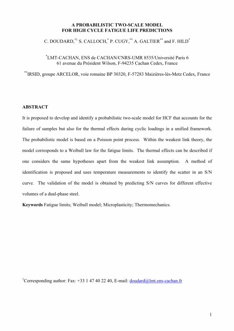
where ( ) ( ) dttexptpΓ0

1p∫ −=∞

− is the gamma function [40]. These two relationships can be used to

evaluate the coefficient of variation

+

+−

+

=

m11Γ

m11Γ

m21Γ

CV

2

(32)

that only depends on the Weibull modulus, i.e., it characterizes the scatter. Equation (30) accounts

for scale effects associated to the Weibull model [41]. Namely, the higher the loaded volume, the

smaller the mean fatigue limit; the higher the stress heterogeneity (i.e., the smaller Hm), the higher

the mean fatigue limit. These coupled effects are described by the introduction of the so-called

effective volume Veff = VΩHm [5]. Consequently corrections are to be performed when comparing

data of samples tested in tension/compression to those of structures for which the stress field is

different as well as the loaded volume. This analysis is relevant when initiation occurs within the

volume as observed for dual-phase steels [22]. Had initiation occurred at or close to the surface, an

effective surface instead of an effective volume should have been used.

In the following analysis, the heat transfer analysis is performed again. However, the

weakest link hypothesis is not considered since it is assumed that the gradual temperature change is

associated with the gradual microplastic dissipation corresponding to a random distribution of yield

stresses. The underlying Poisson point process as well as the power law of its intensity are still

used. With a Poisson point process, dΣVdλd

ΩΣ is the mean number of inclusions activated

between an equivalent stress Σ and Σ+dΣ in a domain of volume VΩ, i.e. the number of sites whose

mean fatigue limit lies between Σ and Σ+dΣ, and whose dissipated energy VRVED(Σ) during a load

cycle is given by

ΣΣΣh

4V)D(V 0

0RVE −=Σ . (33)

13

For a specimen of volume VΩ, the global dissipated energy density ∆ for an equivalent stress

amplitude Σ0 during a load cycle is expressed as

dΣΣdλd)(DV

0Σ

0RVE∫ Σ=∆ , (34)

so that

( )( ) ( )m0

1/m0

2m00

SV

Σ2m1m

mhV4 +

++=∆ . (35)

The change of the mean steady-state temperature is obtained by the resolution of the heat

conduction equation (21) by using ∆ instead of D

( ) ( ) ( )m01/m0

2m0

0SV

Σ2m1m

mVηθ+

++= . (36)

Equation (36) does not show a sudden change of the mean steady-state temperature with the stress

amplitude but rather a gradual increase in accordance with Fig. 6. The present model is dependent

on three parameters, namely, ηV0, ( ) m/100 VS and m. The influence of the parameters on the

change of the steady-state temperature is described in Figs. 6:

• the smaller the scale parameter of the Weibull-model ( ) m/100 VS , the sooner the increase of

temperature (Fig. 6a);

• the smaller the scale parameter of the temperature variation ηV0, the later the increase of

temperature (Fig. 6b);

• the smaller the Weibull modulus m, the more gradual the increase of the temperature (Fig.

6c).

The parameters ( ) m/100 VS and ηV0 appear simultaneously in the model. Therefore their

identification requires two independent measurements, namely temperature measurements and the

classical Wöhler (S/N) curve.

14

4. Identification procedure and predictions

In the following, the different parameters are identified: namely, ( ) m/100 VS characterizes the level

of the mean fatigue limit for an effective volume equal to V0, ηV0 is a parameter depending on

material to describe the temperature kinetics, m measures the scatter of the fatigue limits, and A

characterizes the initiation criterion. First, the parameters A and ∞Σ are identified by using the

classical Wöhler curve and Stromeyer's law

∞∞ Σ⟩ΣΣ⟨=

-A N

0, (37)

where 15 samples are usually needed. Then the values for m and ηV0 are determined from the

analysis of the temperature measurements (Eqn. (36)) for which an additional sample is used. The

results of the identification are shown in Fig. 7. The temperature measurements are better described

than with the deterministic approach (Fig. 5), especially in the transition regime. The scale

parameter ( ) m/100 VS is obtained by using the expression (30) of the mean fatigue limit for

samples with an effective volume equal to Veff = 620 mm3 (see Appendix A).

The first validation concerns the prediction of the scatter of the experimental fatigue result

in tension/compression (load ratio R = -1). The number of cycles to failure is related to the stress

amplitude Σ0 and failure probability by using Stromeyer's law associated to each fatigue limit

)P()P(-A N

FF0 ∞∞ Σ⟩ΣΣ⟨= (38)

where )P( F∞Σ is the fatigue limit for the failure probability FP . This limit can be written as

mFF

(0.5))P(

) 0.5-1 (ln )P - 1 (ln

ΣΣ

=∞

∞ (39)

by assuming that ∞∞∞ Σ≈

+Σ=Σ )

m1Γ(1/ln(2)(0.5) m

1

(the higher m, the better the

approximation). Figure 8a shows the comparison between the experimental results obtained by

15

classical fatigue tests and the prediction of the model for three different failure probabilities. The

Wöhler curves can be predicted in a reasonable way.

The second validation concerns the prediction of the Wöhler curve for the same dual-phase

steel loaded in alternate bending (R = -1). It is worth noting that no new parameters are needed to

obtain the predictions. Figure 8b shows the comparison between the experimental results and the

prediction of the model for bending tests (Veff = 13 mm3). The general trend of the constant failure

probabilities is in good agreement with the experimental results and the scatter is reasonably

predicted. A Weibull modulus of 20 was identified from the thermal test so that the standard

deviation of the fatigue limit is equal to 16.5 MPa by using Eqn. (32) and the value MPa275=Σ∞ .

Since the effective volume is significantly different (i.e., 30 times smaller) from the axial

tension/compression tests, the average fatigue limit in bending is greater than that in axial tension

compression. This result is another validation of the probabilistic approach developed herein. For

higher stress levels, the predictions become conservative. An explanation may be related to the fact

that generalized plasticity occurs in addition to the fact that the propagation stage, which is not

described herein, may become more significant.

5. Conclusions

The present analysis of the thermal effects during cyclic loadings is related to microplasticity, when

the volume of the elasto-plastic inclusions is very small when compared to the volume of the tested

sample and when the temperature of the sample can be considered homogenous. If a deterministic

model is considered, the mean fatigue limit can be determined by this test. In terms of high cycle

fatigue, the same model allows for the identification of a Wöhler curve by using Stromeyer's law.

The probabilistic model presented herein for HCF life predictions is based on a Poisson

point distribution of the sites where microplasticity takes place. Within the weakest link theory, the

model corresponds to a Weibull law for the fatigue limits. Within the same set of hypotheses, apart

from the weakest link assumption, the thermal effects can be described and a gradual change of the

16

steady-state temperature with the applied stress amplitude is obtained. The thermal effects are

accurately reproduced by the model for a dual-phase steel. In particular, the scatter in HCF can be

identified by this test.

A method of identification applicable in HCF is proposed and uses temperature

measurements. One sample only is needed to identify the scatter by using temperature

measurements and 15 samples to identify the classical Wöhler curve, here described by Stromeyer’s

law instead of 30 to 50 samples when the scatter in HCF is sought. The failure probability can be

predicted by the model for different effective volumes. The validation of the model is obtained for

the prediction of S/N curves for different effective volumes corresponding to axial and bending

fatigue tests.

6. Acknowledgments

This work was performed within a collaboration with ARCELOR and Nippon Steel Corporation.

7. References

[1] W. Weibull (1961) Fatigue testing and analysing of results. Pergamon Press, Oxford (UK).[2] A. Brand, J. F. Flavenot, R. Grégoire and C. Tournier (1992) Données technologiques sur la

fatigue. Publications CETIM, Senlis (France).[3] W. Weibull (1949) A statistical representation of fatigue failures in solids. Trans. Roy.

Swed. Inst. Tech. 27.[4] F. Bastenaire (1960) Étude statistique et physique de la dispersion des résistances et des

endurances à la fatigue. Thèse d'État, Université de Paris.[5] D. G. S. Davies (1973) The Statistical Approach to Engineering Design in Ceramics. Proc.

Brit. Ceram. Soc. 22, 429-452.[6] F. Hild, A.-S. Béranger and R. Billardon (1996) Fatigue Failure Maps of Heterogeneous

Materials. Mech. Mater. 22, 11-21.[7] H. Yaacoub Agha, A.-S. Béranger, R. Billardon and F. Hild (1998) High Cycle Fatigue

Behaviour of Spheroidal Graphite Cast Iron. Fat. Fract. Eng. Mater. Struct. 21, 287-296.[8] I. Chantier, V. Denier-Bobet and F. Hild (2000) A Lifing Procedure for Shot-Peened Cast

Components Subjected to High Cycle Fatigue. ECF13, CD-ROM, Elsevier, Oxford (UK),(3C.127) 8 p.

[9] M. P. Luong (1992) Infrared thermography of fatigue in metals. SPIE 1682, 222-233.[10] J.-Y. Bérard, S. Rathery and A.-S. Béranger (1998) Détermination de la limite d’endurance

des matériaux par thermographie infrarouge. Mat. Techn. 1-2, 55-57.[11] J.-C. Krapez, D. Pacou and C. Bertin (1999) Application of lock-in thermography to a rapid

evaluation of the fatigue limit in metals. 5th AITA, Int. Workshop on Advanced InfraredTechn. and Appl., Venezia (Italy), Ed. E. Grinzato et al., 379-385.

[12] G. La Rosa and A. Risitano (2000) Thermographic methodology for rapid determination ofthe fatigue limit of materials and mechanical components. Int. J. Fat. 22 [1], 65-73.

17

[13] C. Mabru and A. Chrysochoos (2001) Dissipation et couplages accompagnant la fatigue dematériaux métalliques. Photomécanique 2001, Ed. Y. Berthaud, M. Cottron, J.-C. Dupré, F.Morestin, J.-J. Orteu and V. Valle, GAMAC, 375-382.

[14] A. Galtier, O. Bouaziz and A. Lambert (2002) Influence de la microstructure des aciers surleurs propriétés mécaniques. Méc. Ind. 3 [5], 457-462.

[15] J. Lemaitre and I. Doghri (1994) Damage 90: a post processor for crack initiation. Comput.Methods Appl. Mech. Engrg. 115, 197-232.

[16] J. Lemaitre, J.-P. Sermage and R. Desmorat (1999) A two scale damage concept applied tofatigue. Int. J. Fract. 97, 67-81.

[17] G. R. Speich and R. L. Miller (1979) Structure and properties of dual phase steels. Ed. R. A.Kot and J. W. Morris, AIME, New York (USA), 146-181.

[18] Z. Li, J. Han, Y. Wang and Z. Kuang (1990) Low-cycle fatigue investigations and numericalsimulations on dual phase steel with different microstructures. Fat. Fract. Eng. Mat. Struct. 3[3], 229-240.

[19] A. Gustavsson and A. Melanger (1994) Variable-amplitude fatigue of a dual-phase sheetsteel subjected to prestrain. Int. J. Fat. 16, 503-509.

[20] T. C. Lei, G. Y. Lin and Y. X. Cui (1994) Dislocation substructures in ferrite of plain carbondual-phase steels after fatigue fracture. Fat. Fract. Eng. Mat. Struct. 17 [4], 451-458.

[21] T. M. Hashimoto and M. S. Pereira (1996) Fatigue life studies in carbon dual-phase steels.Int. J. Fat. 18 [8], 529-533.

[22] K. Nakajima, S. Kamiishi, M. Yokoe and T. Miyata (1999) The influence of microstructuralmorphology and prestrain on fatigue crack propagation of dual-phase steels in the near-threshold region. ISIJ International 39 [5], 486-492.

[23] M. Sarwar and R. Priestner (1999) Fatigue crack propagation behaviour in dual phase steel.J. Mat. Eng. Perform. 8, 245-251.

[24] Z. G. Wang and S. H. Ai (1999) Fatigue of martensite-ferrite high strength low alloy dualsteels. ISIJ international 39 [8], 747-759.

[25] M. E. Haque and M. S. Sudhakar (2001) ANN based prediction model for fatigue crackgrowth in DP steel, ". Fat. Fract. Eng. Mat. Struct. 23, 63-68.

[26] A. Chrysochoos and H. Louche (2000) An infrared image processing to analyse the calorificeffects accompanying strain localisation. Int. J. Eng. Sci. 38, 1759-1788.

[27] J. Lemaitre and J.-L. Chaboche (1990) Mechanics of Solid Materials. Cambridge UniversityPress, Cambridge (UK).

[28] M. Berveiller and A. Zaoui (1979) An extension of the self-consistent scheme to plasticallyflowing polycrystals. J. Mech. Phys. Solids 26, 325-344.

[29] E. Kröner (1984) On the plastic deformation of polycristals. Acta Met. 9, 155-161.[30] J. D. Eshelby (1957) The Determination of the Elastic Field of an Ellipsoidal Inclusion and

Related Problems. Proc. Roy. Soc. London A 241, 376-396.[31] P. Germain, Q. S. Nguyen and P. Suquet (1983) Continuum Thermodynamics. ASME J.

Appl. Mech. 50, 1010-1020.[32] E. Charkaluk, A. Bigonnet, A. Constantinescu and K. Dang Van (2002) Fatigue design of

structures under thermomechanical loadings. Fat. Fract. Eng. Mat. Struct. 25 [12], 1199-1206.

[33] C. E. Stromeyer (1914) The determination of fatigue limits under alternating stressconditions. Proc. Roy. Soc. London A90, 411-425.

[34] A. B. De Vriendt (1987) La transmission de la chaleur. Morin, Québec (Canada).[35] R. Gulino and S. L. Phoenix (1991) Weibull Strength Statistics for Graphite Fibres

Measured from the Break Progression in a Model Graphite/Glass/Epoxy Microcomposite. J.Mater. Sci. 26 [11], 3107-3118.

[36] D. Jeulin (1991) Modèles morphologiques de structures aléatoires et changement d'échelle.Thèse d'État, Université de Caen.

18

[37] W. Weibull (1939) A Statistical Theory of the Strength of Materials. Roy. Swed. Inst. Eng.Res., Report 151.

[38] W. Weibull (1951) A Statistical Distribution Function of Wide Applicability. ASME J.Appl. Mech. 18 [3], 293-297.

[39] F. Hild, R. Billardon and D. Marquis (1992) Hétérogénéité des contraintes et rupture desmatériaux fragiles. C. R. Acad. Sci. Paris t. 315 [Série II], 1293-1298.

[40] M. Abramowitz and I. A. Stegun (1965) Handbook of Mathematical Functions. DoverPublications, Inc., New York (USA).

[41] W. Weibull (1952) A Survey of 'Statistical Effects' in the Field of Material Failure. Appl.Mech. Rev. 5 [11], 449-451.

19

Appendix A: computation of the effective volume

This appendix aims at detailing the calculation of the effective volume defined by

meff HVV Ω= (A1)

where dVΣΣ

V1H

m

FΩm ∫

= is the stress heterogeneity factor and ( )ΣmaxΣF Ω= . The geometry

of tensile and bending samples is defined in Fig. A1. For the tensile test the stress Σ depends only

on the height y and the cross-sectional area varies with y as

−−+=

2

00 R

y11l2R1lS(y) e (A2)

so that the stress heterogeneity factor reads

dy

Ry11

l2R1

1y1H

0y

0m

2

0

0m ∫

−−+

= (A3)

where )2(y0 dRd −= .

For the bending test, Σ depends on y and z. The dependence with y is calculated as for the

tensile test and the dependence with z is linear. Consequently, when the load ratio is equal to -1, the

stress heterogeneity factor is expressed as

dz2dy

Ry11

l2R1

1ey

2He/2

0

m0y

0m

2

0

0m ∫

∫

−−+

=ez (A4)

20

List of tables

Table 1: Chemical composition of the DP600 steel (10-3 wt%)

Table 2: Mechanical properties of the DP600 steel (Ys = Yield stress, UTS = Ultimate Tensile

Strength, El = Elongation at failure).

21

Table 1. Doudard et al.

C Mn Si Cr Ti S Fe120 1400 350 200 10 < 5 Balance

Table 2. Doudard et al.

Ys UTS Ys / UTS El> 300 MPa > 600 MPa < 0.6 25 %

22

List of figures:

Figure 1: thermal effects for a dual-phase DP600 steel: -a-cyclic loadings, -b-successive series of

3000 cyclic loadings for different increasing stress amplitudes Σ0, -c-change of the temperature

during 3000 cyclic loadings for the same stress amplitude -d-change of the steady-state mean

temperature with the load amplitude.

Figure 2: RVE of the two-scale model.

Figure 3: S/N curve of the studied dual-phase steel (Σm = 0).

Figure 4: analysis of the thermal boundary conditions during the study of the thermal effects for the

considered gauge volume.

Figure 5: identification of η and ∞Σ for the studied dual-phase steel (fr = 10 Hz, Σm = 0).

Figure 6: change of θ with Σ0: -a-influence of ηV0 with m=20 and S0(V0)1/m =390MPa.mm3/20 , -b-

influence of S0(V0)1/m with m=20 and ηV0 =0.49K.MPa-2, -c-influence of m with ηV0=0.49K.MPa-2

and S0(V0)1/m =390MPa.mm3/20.

Figure 7: identification of A and ∞Σ (-a-) from the classical Wöhler curve, ηV0 and m from

temperature measurements (-b-) for the studied dual-phase steel (fr = 10 Hz, Σm = 0).

23

Figure 8: comparison between the prediction of the probabilistic model and the experimental results

for the studied dual-phase steel (Σm = 0) -a-tensile fatigue test -b-bending fatigue test. The same

stress amplitude is shown.

Figure A1: tensile and bending fatigue samples for the studied dual-phase steel with e = 1.5 mm

(tensile sample: R = 100 mm, l0 = 18 mm and d = 9 mm; bending sample: R = 42.5 mm, l0 = 20 mm

and d = 5 mm).

24

Σ0

Σ(MPa)

timef

r-1

Σm

Σ0

Σ0n

Σ0i

Σ01

cycles30000

sucessiveseries

9000

- a - - b -

cycles

θ

θ(K)Σ

0=280MPa

0 1500 30000

0.4

0.2

0.6

-0.5

0

0.5

1

1.5

2

0 50 100 150 200 250 300

θ(K)

Σ0(MPa)

specimen 2specimen 1

material: dual-phasef

r = 10Hz, Σ

m= 0

- c - - d -

Figure 1. Doudard et al.

25

Figure 2. Doudard et al.

Elasto-plastic inclusion

Elastic matrixΕΣ,

εσ ,

26

260

270

280

290

300

310

320

330

104 105 106 107

number of cycles to failure

no failure

Σ0(MPa) material : dual-phase

Σm=0

Figure 3. Doudard et al.

27

l

L

e

heat exchange with the upper grip: h

2 (T-T

0) e.l

heat exchange with surrounding air:

2 h1 (T-T0) L.(e + l)

heat exchange with the lower grip: h

2 (T-T

0) e.l

Figure 4. Doudard et al.

28

-0.5

0

0.5

1

1.5

2

0 50 100 150 200 250 300

η fv= 2.3 10-4 K.MPa-2

Σ0(MPa)

θ(K)

Σ = 274MPa

material : dual-phasef

r = 10Hz, Σ

m= 0

8Figure 5. Doudard et al.

29

θ(K)η

1V

0 = 0.49 K.MPa-2

η2V

0 = 9.8 K.MPa-2

Σ0(MPa)

θ(K)S

01V

0

1/m = 390 MPa.mm3/20

Σ0(MPa)

S02

V0

1/m = 330 MPa.mm3/20

Σ0(MPa)

θ(K)

m2 = 12

m1 = 20

-a- -b- -c-

Figure 6. Doudard et al.

30

260

280

300

320

340

104 105 106 107

A = 1.2 109 MPa2

material : dual-phaseΣ

m=0

number of cycles to failure

Σ0(MPa)

Σ = 275MPa8

-0.5

0

0.5

1

1.5

2

0 50 100 150 200 250 300

m = 20

η V0= 1.1 10-1 K.MPa-2mm3

θ(K)

Σ0(MPa)

material : dual-phasefr = 10Hz, Σ

m= 0

-a- -b-

Figure 7. Doudard et al.

31

240

260

280

300

320

340

360

380

400

104 105 106 107

number of cycles to failure

no failureP

F=50%

PF=20%

PF=80%

Model

∆Σ(MPa) material : dual-phase Σ

m= 0

240

260

280

300

320

340

360

380

400

104 105 106 107

no failure

PF=50%

PF=20%

PF=80%

Model

∆Σ(MPa)

number of cycles to failure

material : dual-phaseΣ

m= 0

-a- -b-

Figure 8. Doudard et al.

32

Figure A1. Doudard et al.

l0

R

d e