Embed Size (px)
Citation preview

Helsinki University of Technology publications in Power Systems 7
Espoo 2003 TKK-SVL-7
A PROBABILISTIC METHOD FOR COMPREHENSIVE VOLTAGE
SAG MANAGEMENT IN POWER DISTRIBUTION SYSTEMS
Pasi Pohjanheimo


Helsinki University of Technology publications in Power Systems 7
Espoo 2003 TKK-SVL-7
A PROBABILISTIC METHOD FOR COMPREHENSIVE VOLTAGE
SAG MANAGEMENT IN POWER DISTRIBUTION SYSTEMS
Pasi Pohjanheimo Dissertation for the degree of Doctor of Technology to be presented with due permis-
sion for public examination and debate in Auditorium S5 at Helsinki University of
Technology (Espoo, Finland) on the 20th of October, at 12 o’clock noon.
Helsinki University of Technology
Department of Electrical and Communications Engineering
Power Systems Laboratory

Distribution:
Helsinki University of Technology
Power Systems Laboratory
P.O. Box 3000
FIN-02015 HUT
FINLAND
Tel. + 358 9 4511
E-mail: [email protected]
© Pasi Pohjanheimo
ISBN 951-22-6398-X
ISBN 951-22-6399-8 (PDF)
ISSN 1458-9249
Otamedia Oy
Espoo 2003

ABSTRACT OF DOCTORAL THESIS Helsinki University of Technology
P.O.Box 1000, FIN-02015 HUT
http://www.hut.fi/ Author: Pasi Pohjanheimo Name of the thesis: A probabilistic method for comprehensive voltage sag management in power distribution systems Date of dissertation: October 20th, 2003 Type of thesis: Monograph
Department: Department of Electrical and Communications Engineering Laboratory: Power Systems Laboratory Field of research: Power Quality Opponents: Dr. Jovica V. Milanovic & Dr. Anssi Seppälä Pre-examiners: Prof. Kimmo Kauhaniemi & Dr. Anssi Seppälä
Supervisor: Prof. Matti Lehtonen Abstract:
Voltage sags, their technical and economic impact and the means of their mitiga-tion have become popular topics for discussion, publication and R&D projects within the power engineering society. However, a tool including and combining analysis of all these fields in a simple yet mathematically exact way has not been proposed.
This thesis outlines a probabilistic method for comprehensive voltage sag manage-ment named Prob-A-Sag. All quantities are processed as probabilistic two-dimensional arrays. Multiplying the arrays cell by cell gives the total annual sag related cost. Further, the optimal type and rating of a mitigation device can be assessed.
Remaining voltage and sag duration are the variables considered in the arrays. Array resolution and thus the procedure accuracy are freely selectable. Increasing the number of dimensions allows for additional sag features, e.g. unbalance and phase-angle jump could be included in a future enhancement of the method.
A probabilistic approach, one of the key features of the method, is essential when as-sessing the performance of multiple similar sag sensitive components connected to-gether. It also proved useful in cases where specific device sensitivity tests cannot be carried out but instead, generalised data from previously prepared libraries has to be used to assess the entire process sensitivity.
In addition to this method, the thesis provides sag sensitivity test results for contac-tors, personal computers and gas discharge lamps. Discussion and calculations on the feasibility and network requirements of custom power technology are also included. Keywords: Voltage sags, Power quality, Power distribution UDC: 621.3 Number of pages: xii + 87 ISBN: 951-22-6398-X ISBN (PDF): 951-22-6399-8 Series: Helsinki University of Technology publications in Power Systems ISSN: 1458-9249 Report nr.: TKK-SVL-6 Report nr. (PDF): TKK-SVL-7
Publisher and print distributor: Helsinki University of Technology Power Systems Laboratory The full manuscript is available at: http://lib.hut.fi/Diss/
i

ii

PREFACE
The research work related to this thesis has been carried out in the Power Sys-tems Laboratory of Helsinki University of Technology during the years 1999-2003 as a natural continuum from the master’s thesis by the author. In addition to the university, the TESLA technology programme by TEKES, the Power systems re-search pool coordinated by Finergy, the Graduate School in Electrical Engineer-ing and the Sähköinsinööriliiton säätiö have provided the financial basis for the project.
Professor Erkki Lakervi supervised the beginning of the work. Professor Matti Lehtonen took over from him after two years. Them both I want to warmly thank for providing excellent facilities for testing and measurements as well as sharing their time, expertise and guidance. Moreover, to Professor Lehtonen I would like to express my deepest gratitude for his patience and gentle pressure to accomplish the thesis.
The pre-examiners of the thesis, Professor Kimmo Kauhaniemi and Doctor Anssi Seppälä, gave valuable comments on the first version of the manuscript.
The personnel of the Power Systems Laboratory have been of great help and support both mentally and with practical issues throughout the period. The benign daily joking and banter along the lab corridor has been an outstanding source of good humour and revitalization for the night shift zombie. Thanks, folks!
Pirjo Heine - who has been sharing not only the office with me but, without be-ing given a chance to refuse, also the pain often present in a creative process like this - absolutely deserves to be acknowledged here by name. The room arrange-ment has also enabled fruitful and productive academic discussion across the screen separating our desks.
John Millar, also a colleague of mine, invariably consented to answer those “an-other questions” concerning the language issues. I appreciate his work in proof-reading the manuscript and willingly engaging in an interactive and iterative proc-ess, which eventually achieved an outcome beyond my highest expectations.
A significant number of people, way too many to be mentioned here by name, have contributed, co-operated and supported my journey towards something I never thought would be possible to attain. Without you that could have well been the case. Thank you all so much.
And finally, my beloved redhead Kirsimari. She has hugged me back to life so many times during the arduous slog - and thereby has certainly qualified for wifing a scatty and weird scientist! Heartfelt thanks for your love, care and patience.
In Espoo, September 29th, 2003 a.D.
Elimu ni maisha, si vitabu.
iii

iv
TABLE OF CONTENTS
ABSTRACT OF DOCTORAL THESIS......................................................... i PREFACE ............................................................................................... iii TABLE OF CONTENTS.............................................................................v LIST OF SYMBOLS AND ABBREVIATIONS ..........................................vii 1 INTRODUCTION ................................................................................... 1 2 VOLTAGE SAGS IN A POWER DISTRIBUTION SYSTEM ................... 2
2.1 Definition ....................................................................................... 2 2.2 Cause of voltage sags ...................................................................... 2 2.3 Frequency of voltage sags ............................................................... 7 2.4 Three-phase characterization of voltage sags ................................... 8
3 TECHNICAL AND ECONOMIC IMPACTS........................................... 10
3.1 Technical aspects.......................................................................... 10 3.1.1 Contactors ............................................................................ 11 3.1.2 Gas discharge lamps.............................................................. 17 3.1.3 Microprocessor based equipment ........................................... 20 3.1.4 Converters ............................................................................ 22
3.2 Economic aspects ......................................................................... 25 4 MITIGATION OF VOLTAGE SAGS ..................................................... 28
4.1 Custom power technology.............................................................. 28 4.1.1 Transfer switch ..................................................................... 29 4.1.2 Series power conditioner with energy storage ......................... 35 4.1.3 Series power conditioner without energy storage .................... 41
4.2 Other means of mitigation ............................................................. 44 5 PROB-A-SAG METHOD ...................................................................... 45
5.1 Existing methods .......................................................................... 45 5.2 Objectives for novel method........................................................... 47 5.3 Processing the arrays.................................................................... 49 5.4 Probabilistic approach .................................................................. 51 5.5 Analysing a complete process ........................................................ 53 5.6 Cost assessment ............................................................................ 57 5.7 Mitigation devices......................................................................... 61 5.8 Summary ..................................................................................... 67
v
6 APPLICATION EXAMPLES................................................................69
6.1 Example I .....................................................................................69 6.2 Example II....................................................................................71
7 DISCUSSION.......................................................................................76 8 CONCLUSION......................................................................................78 REFERENCES........................................................................................79 APPENDIX A – Detailed model of a series power conditioner .................82
vi

LIST OF SYMBOLS AND ABBREVIATIONS
∀ for all
∋ such that
A ampere
AC, ac alternating current
c cycle
C total annual sag related cost
CBEMA Computer and Business Equipment Manufacturers Associa-tion
CP custom power (technology)
D(i,j) device sensitivity array
DC, dc direct current
DKK Danish Crown
Dn(i,j) device sensitivity array of device n
Dr. doctor
DSP digital signal processing
dt differential operator in relation to time
du differential operator in relation to voltage
DVR dynamic voltage restorer
€ euro
E energy
E(i,j) event cost array
Einj injected energy
EMC electromagnetic compatibility
vii

Hg mercury (lamp)
HPS high-pressure sodium (lamp)
HV high voltage
Hz hertz
I(i,j) annual interruption frequency array
I(u), I(u,t) risk of sag related interruption
IC integrated circuit
IEC The International Electrotechnical Commission
IEEE The Institute of Electrical and Electronics Engineers
Il load current
Il* complex conjugate of load current Il
ITI Information Technology Industry Council
j imaginary unit
k integer
kA kiloampere
k€ thousand euros
keV kiloelectronvolt
kJ kilojoule
km kilometre
kV kilovolt
kVA kilovoltampere
kVAr reactive kilovoltampere
kW kilowatt
L1, L2, L3 phases of a 3-phase ac power system
viii

LV low voltage
m integer
max maximum
med median
MeV megaelectronvolt
MH metal halide (lamp)
min minimum
ms millisecond
MV medium voltage
MVA megavoltampere
N total annual number of sag related interruptions
n integer
P active power
p probability
P(i,j) process sensitivity array
P(u), P(u,t) process sensitivity
PC personal computer
PCC point of common coupling
Pinj injected active power
Pl active power drawn by the load
PLC programmable logic controller
PQ power quality
Ps active power drawn from the sagged supply
p.u. per unit
Q reactive power
ix

q integer
Qinj injected reactive power
Ql reactive power drawn by the load
Qs reactive power drawn from the sagged supply
r integer
R(i,j) restored annual sag frequency array
RMS, rms root mean square
s second
S(i,j) annual sag frequency array
S(u), S(u,t) annual frequency of voltage sags
SF6 sulphur hexafluoride
SFS-EN Finnish Standards Association – European Norm
Sinj injected apparent power
Sl load apparent power
SMES superconducting magnetic energy storage
SSTS solid-state transfer switch
t time
tcrit critical duration of a voltage sag
tj
- lower limit of time category j
tj
+ upper limit of time category j
U, u voltage
UBUS busbar voltage
Ucrit critical remaining voltage during voltage sag
Ui
- lower limit of voltage category i
Ui
+ upper limit of voltage category i
x
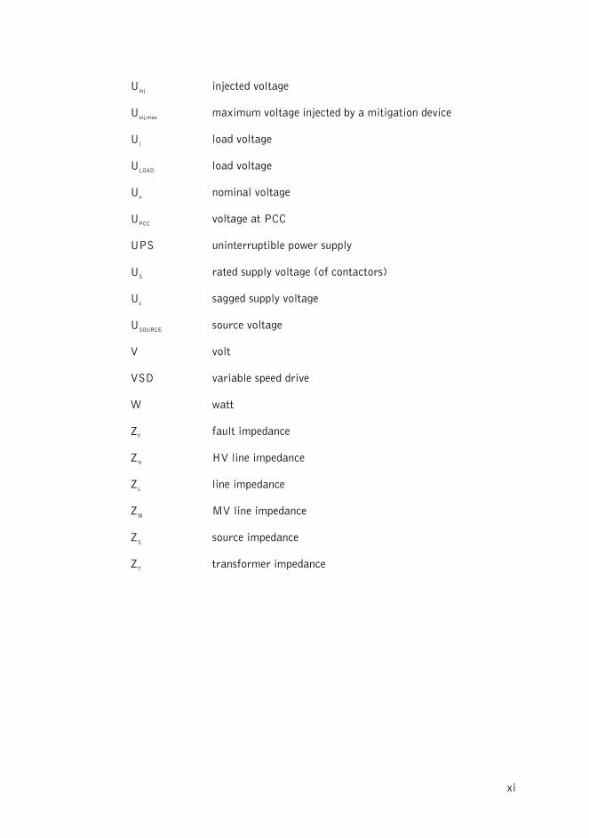
Uinj injected voltage
Uinj,max maximum voltage injected by a mitigation device
Ul load voltage
ULOAD load voltage
Un nominal voltage
UPCC voltage at PCC
UPS uninterruptible power supply
US rated supply voltage (of contactors)
Us sagged supply voltage
USOURCE source voltage
V volt
VSD variable speed drive
W watt
ZF fault impedance
ZH HV line impedance
ZL line impedance
ZM MV line impedance
ZS source impedance
ZT transformer impedance
xi

xii
1 INTRODUCTION
The significance of voltage sags among power quality related phenomena seems to be increasing rapidly. Their impact as randomly timed and randomly shaped events makes them a special challenge for power distribution engineering. From an economic point of view, sags are definitely a problem worth studying and, in most cases, are also worth being solved. Economic losses due to sags are espe-cially high for industrial customers. In many countries the phenomenon and its consequences have only recently been noticed.
However, there are no proper tools for comprehensive voltage sag management, i.e. for assessing and mitigating the inconvenience due to sags as well as for finding the optimal solution for corrective measure(s).
The objective of this thesis is to develop a new probabilistic approach for voltage
sag management in power distribution systems. The major aim in developing the method is to provide the distribution system
community – including planning, operation, software development and financial staff – with a practical, yet theoretically convincing tool for their everyday work.
This tool should comprehensively cover the technical and economic aspects re-lated to voltage sags as well as be able to meet the future challenges set by the issue in a most flexible and adaptive way.
1

2 VOLTAGE SAGS IN A POWER DISTRIBUTION SYSTEM
Ideally, a power distribution system provides its customers with an uninter-rupted flow of energy at unlimited power rating having smooth sinusoidal voltage at the contracted magnitude level and frequency.
In reality, a power system has numerous non-ideal features which significantly affect the quality of power. Voltage sags also originate from these anomalies. It is impossible to completely avoid sags but they are events that we can live with pro-vided that the phenomenon is understood and taken into account.
2.1 Definition
This thesis considers voltage sags in power distribution systems. The European norm EN 50160 (2000-01-24) “Voltage characteristics of electricity supplied by public distribution systems” [1] applies to distribution systems in Europe. This norm also has the status of a Finnish national standard (SFS). In the publication, a voltage sag (or dip) is defined as a sudden reduction of supply voltage down to 90 %…1 % of nominal followed by a recovery after a short period of time. A typical duration of a sag is, according to the standard, 10 ms to 1 minute.
IEEE Std. 1159-1995, the IEEE recommended practice for monitoring electric power quality [2], gives somewhat similar values (magnitude 90 % to 10 %, dura-tion 10 ms to 1 minute) as a definition of voltage sag.
The type of event considered in the thesis is sometimes called a voltage dip and on other occasions a voltage sag. Technically these two terms describe exactly the same phenomenon. Thus from this point on the expressions voltage sag and sag will be used to avoid confusion.
Another thing that needs to be defined is the magnitude or depth of a sag. Of-ten the remaining voltage during a sag is used to describe its severity whereas some people prefer to speak of the missing voltage instead. Even though it is a subjective matter, the latter alternative is more complicated and has a higher risk of misinter-pretation than the former one. In this thesis, the expression sag magnitude refers to the remaining supply voltage during a voltage sag. Further, deep sag refers to sags that have small a remaining voltage and shallow sag to ones with high remaining voltage.
2.2 Cause of voltage sags
Generally, voltage sags experienced by distribution system customers originate from the (HV) transmission and sub-transmission systems, or the (MV) distribution system itself. In the case of weak transmission systems it is also possible to get sags
2

from neighbouring MV distribution systems through the transmission network.
Fig. 2.1. Example of distrib
Fig. 2.1 gives an example.
ution of sags propagating from different power system lev-
he ratio of contributions from different voltage levels depends on the struc-tur
ime reason for sags: hig
originate from power system faults. A 3-phase short circuit clo
originate from climatic phenomena (lightning, wind, snow), wil
likely examples of such events.
0
5
10
15
20
25
30
35
40
45
50
<10 <20 <30 <40 <50 <60 <70 <80 <90
Sag magnitude (%)
Sag
fre
quen
cy (
1/a)
MV MV remote HV
els [3]. T
e, protection coordination and stiffness of the various subsystems. Downstream from a strong HV transmission system most sags, especially the deep ones, originate from the MV network. Only a fraction of the sags experienced by a customer are of HV system origin, and most of them are typically shallow.
Disregarding the delivering subsystem(s), there is one prh current flowing through some part(s) of the network. This current induces
voltage drop over network impedances until it is cut off, usually by overcurrent pro-tection. See Fig. 2.2.
Most severe sags se to a distribution substation is capable of bringing the main busbar voltage
down and thus causing a deep sag to all customers supplied by that particular sub-station. Most of the sags due to power system faults are shallower, though. Fig. 2.3 shows an example.
Faults typically dlife (birds, squirrels, beavers, etc.) and component failures. In addition to
faults, significant changes in power flow may cause momentary voltage drops. Starting a large, directly fed motor, energizing a transformer or transferring loads from one supply to another, e.g. during backup supply arrangements, are the most
3
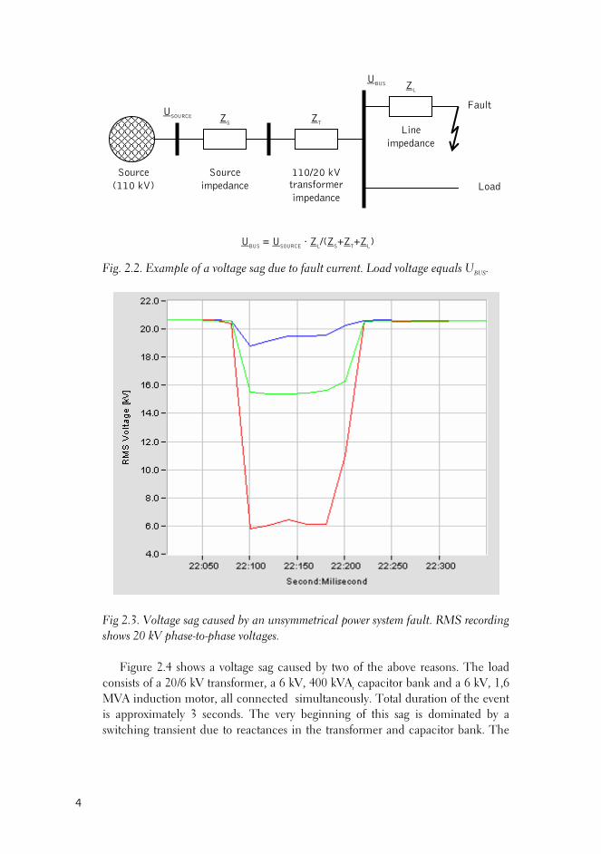
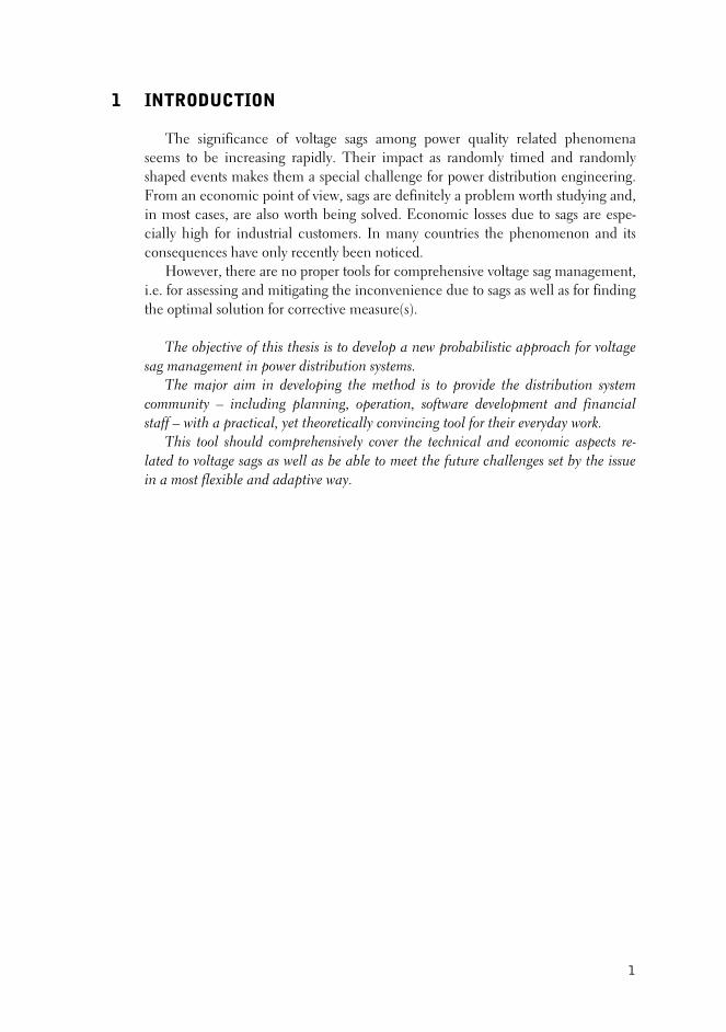
Fig. 2.2. Example of a voltage sa ad voltage equals UBUS.
ing
Figure 2.4 shows a voltage sag caused by two of the above reasons. The load V 1,6
ry beginning of this sag is dominated by a switching transient due to reactances in the transformer and capacitor bank. The
g due to fault current. Lo
USOURCE
Source (110 kV) Load
Fault
Source impedance
110/20 kV transformer
Z
impedance
S Z
T
ZL
Line impedance
UBUS
UBUS
= USOURCE
· ZL/(Z
S+Z
T+Z
L)
Fig 2.3. Voltage sag caused by an unsymmetrical power system fault. RMS recordshows 20 kV phase-to-phase voltages.
consists of a 20/6 kV transformer, a 6 kV, 400 kVAr capacitor bank and a 6 k , MVA induction motor, all connected simultaneously. Total duration of the event is approximately 3 seconds. The ve
4
star
belong to the normal operation of a power system. For this reason only shallow sags
k power systems.
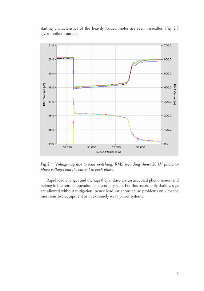
ting characteristics of the heavily loaded motor are seen thereafter. Fig. 2.5 gives another example.
Fig 2.4. Voltage sag due to load switching. RMS recording shows 20 kV phase-to-phase voltages and the current in each phase.
Rapid load changes and the sags they induce are an accepted phenomenon and
are allowed without mitigation, hence load variations cause problems only for the most sensitive equipment or in extremely wea
5
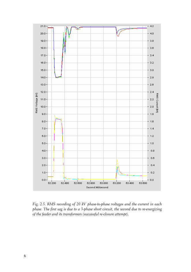
Fig. 2.5. RMS recording of 20 kV phase-to-phase voltages and the current in each phase. The first sag is due to a 3-phase short circuit, the second due to re-energizing of the feeder and its transformers (successful re-closure attempt).
6

2.3 Frequency of voltage sags
From an economic point of view the sag frequency, i.e. the annual number of sags, is very important. Each sag that exceeds the process withstand level intro-duces considerable economic losses. The higher the sag frequency, the higher be-comes the annual cost as well.
When assessing the total annual sag related cost one has to find out how many sags are expected. The difficulty in retrieving the data is its random nature. The annual number of faults depends on numerous random variables.
The ceraunic level (i.e. the number of lightning strokes), wind, rain and snow conditions, even the prevalence of cones (affecting the squirrel population), have significant effects on annual sag numbers. It takes decades, or even centuries, to obtain highly reliable averaged sag density statistics for a certain area.
However, some rough estimation can be acquired from measurement over a shorter period. Another approach is to use stochastic mathematical methods for as-sessing more precise figures.
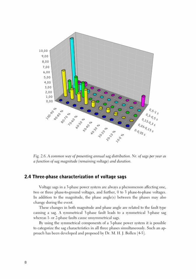
Often the annual sag frequency, or sag distribution, is shown as a three-dimensional chart, like the one in Fig. 2.6. The data is retrieved from actual meas-urements and represents an annual sag frequency in a 20 kV system. Events are first categorised phase by phase. Figures are then summed up category by category and further divided by three, i.e. the number of phases. This way of processing is based on the assumption that events are evenly distributed in each phase. Perform-ing the above mentioned calculations gives us the annual number of sags per phase.
This is a very typical distribution, although the sample is reasonably small. In the time domain there are obvious peaks in three categories, 50-150 ms, 150-300 ms and 300-500 ms. The first one represents the characteristic delays form the in-stant tripping of a circuit breaker in both HV and MV systems. Instant tripping is used when the fault current is higher, in other words, the sags are deeper. This fea-ture can also be seen in the chart. The deepest registered sags are in this time cate-gory.
If the fault current is not very high, an additional delay is allowed in the breaker tripping coordination. Typically this means 300-500 ms. In this time category we can see a high peak at shallow sags. This contribution comes wholly from MV faults. In HV systems, fault currents are reasonably high and thus the faults are usually cleared instantly to avoid component damage. The two deep sags, or actu-ally outages, in the 0,5-1 s category penetrated from the HV system. They were se-vere 3-phase faults which brought the voltages down to zero and tripped a 110 kV line. Automatic backup supply connections took almost a second to arrange. These are very problematic events for sag sensitive devices.
7
100-
90 %
90-8
0 %
80-7
0 %
70-6
0 %
60-5
0 %
50-4
0 %
40-3
0 %
30-2
0 %
20-1
0 %
10-0
%
0-0,05 s
0,05-0,15 s
0,15-0,3 s
0,3-0,5 s
0,5-1 s
0,001,002,00
3,00
4,00
5,00
6,00
7,00
8,00
9,00
10,00
Fig. 2.6. A common way of presenting annual sag distribution. Nr. of sags per year as a function of sag magnitude (remaining voltage) and duration.
2.4 Three-phase characterization of voltage sags
Voltage sags in a 3-phase power system are always a phenomenon affecting one, two or three phase-to-ground voltages, and further, 0 to 3 phase-to-phase voltages. In addition to the magnitude, the phase angle(s) between the phases may also change during the event.
These changes in both magnitude and phase angle are related to the fault type causing a sag. A symmetrical 3-phase fault leads to a symmetrical 3-phase sag whereas 1- or 2-phase faults cause unsymmetrical sags.
By using the symmetrical components of a 3-phase power system it is possible to categorize the sag characteristics in all three phases simultaneously. Such an ap-proach has been developed and proposed by Dr. M. H. J. Bollen [4-5].
8

In the method, sags are divided into four basic types, A, B, C and D. Type A re-fers to symmetrical 3-phase sags, whereas single-phase and phase-to-phase faults cause class B, C or D sags. In Ref. [5], C and D type sags are further divided into three subtypes, e.g. Ca, Cb and Cc, depending on which of the phases, a, b, or c, the fault affected.
In addition to the sag type, a complex phasor called characteristic voltage is all that is needed to describe a voltage sag in a 3-phase system without losing any es-sential information. For systems where the positive and negative impedances are not equal, an additional PN factor (positive-negative factor) is needed in order to ensure accurate results. Any of the phase-to-ground or phase-to-phase voltages dur-ing a sag can be retrieved when the three parameters are known: sag type, charac-teristic voltage and PN factor.
The approach described above is valid also from one voltage level to another because it takes into account transformer and load connections (star-delta), and is based on per unit (p.u.) calculation.
9

3 TECHNICAL AND ECONOMIC IMPACTS
3.1 Technical aspects
Voltage sags can cause serious economic damage to customers. Before we are able to determine the severity of the economic impact we have to determine the technical impact of voltage sags on power distribution system loads. Further, before we can predict the impact of voltage sags on a complete process, plant or service, we have to predict the voltage sag sensitivity of single loads and load types. Because each piece of equipment has a withstand level or curve of its own and, in addition, has a certain amount of randomness in its behaviour, only categorized predictions can reasonably be established. The following chapters give such estimates, i.e. for the impact of voltage sags on some of the most sensitive load types.
There are at least three ways to determine and predict the performance of loads during voltage sags. First there are standards and codes which set the withstand limits for devices connected to a public power system. Manufacturers commit themselves to obeying the standards when designing equipment.
The second way is to collect data from previous surveys done on the topic. Sags seem, however, to be such an emerging issue that comprehensive studies do not yet exist.
The third alternative, one of the academic contributions of this thesis, is to carry out one’s own tests. In the Power Systems Laboratory of Helsinki University of Technology we have successfully set up a testing facility which, among other features, can be used for generating voltage sags of preferred magnitude, waveform, duration and point-on-wave of initiation. The equipment is based on ProfLine 2100, a 3x5 kVA solid-state voltage generator supplied by Schaffner EMV AG, Switzerland, and a DSP (digital signal processing) measuring module. See Fig. 3.1.
One of the great benefits of the system is its capability of reproducing events with exactly the same waveform and parameters. Repeated tests give the results more accuracy. The outcome of our tests compared with previously achieved val-ues and the prevailing standards are represented in the following chapters.
10
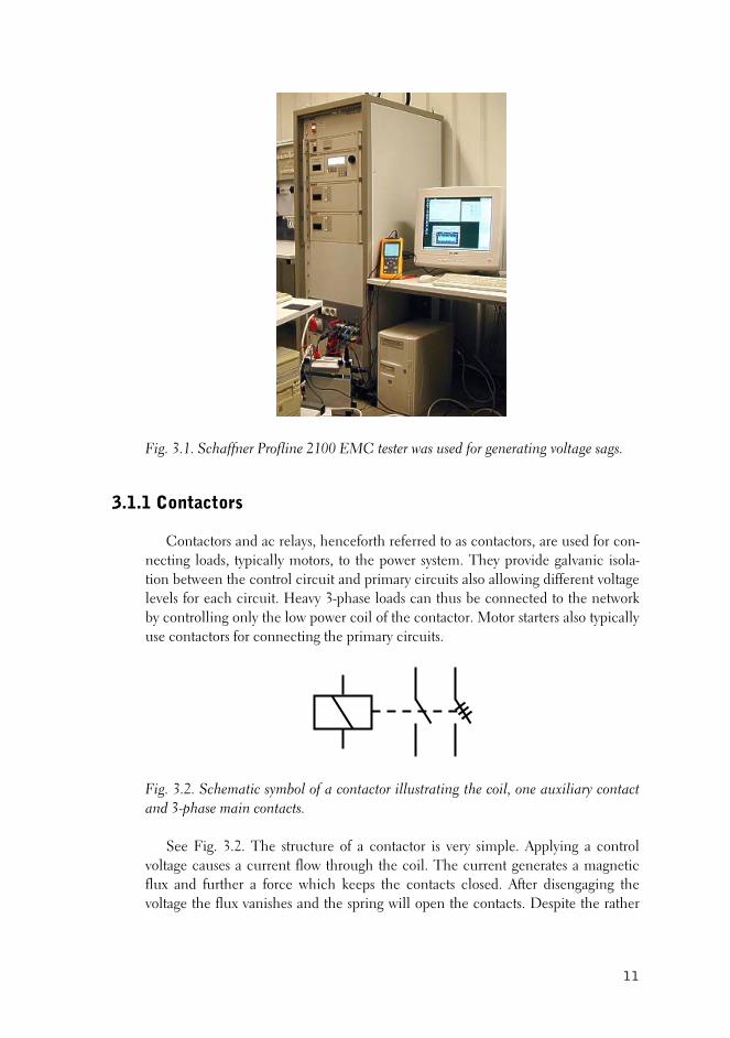
Fig. 3.1. Schaffner Profline 2100 EMC tester was used for generating voltage sags.
3.1.1 Contactors
Contactors and ac relays, henceforth referred to as contactors, are used for con-necting loads, typically motors, to the power system. They provide galvanic isola-tion between the control circuit and primary circuits also allowing different voltage levels for each circuit. Heavy 3-phase loads can thus be connected to the network by controlling only the low power coil of the contactor. Motor starters also typically use contactors for connecting the primary circuits.
Fig. 3.2. Schematic symbol of a contactor illustrating the coil, one auxiliary contact and 3-phase main contacts.
See Fig. 3.2. The structure of a contactor is very simple. Applying a control
voltage causes a current flow through the coil. The current generates a magnetic flux and further a force which keeps the contacts closed. After disengaging the voltage the flux vanishes and the spring will open the contacts. Despite the rather
11
simple and conventional construction, an unintended tripping of a single contac-tor may lead to the shut-down of a sophisticated industrial process. This makes contactors really worth studying from the sag point of view.
Most European contactor manufacturers have designed their products accord-ing to IEC 60947-4-1 [6]. The standard gives the following limits for electromag-netic contactors, whether used separately or in motor starters:
- shall close satisfactorily at any value between 85 % and 110 % of their
rated control supply voltage Us - shall drop out and open fully between 75 % and 20 % of Us for ac, 75 %
and 10 % for dc As can be seen, the limits refer to steady-state conditions. No time limits are
given and thus event type phenomena, e.g. voltage sags, are not specifically consid-ered. One could still expect that the steady state limits are more or less applicable to voltage sags as well.
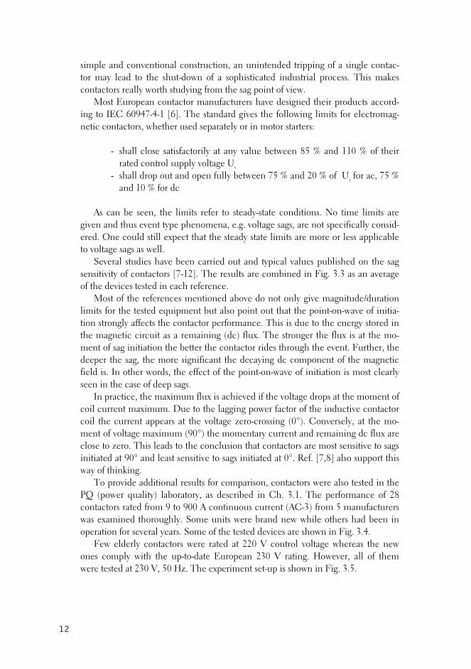
Several studies have been carried out and typical values published on the sag sensitivity of contactors [7-12]. The results are combined in Fig. 3.3 as an average of the devices tested in each reference.
Most of the references mentioned above do not only give magnitude/duration limits for the tested equipment but also point out that the point-on-wave of initia-tion strongly affects the contactor performance. This is due to the energy stored in the magnetic circuit as a remaining (dc) flux. The stronger the flux is at the mo-ment of sag initiation the better the contactor rides through the event. Further, the deeper the sag, the more significant the decaying dc component of the magnetic field is. In other words, the effect of the point-on-wave of initiation is most clearly seen in the case of deep sags.
In practice, the maximum flux is achieved if the voltage drops at the moment of coil current maximum. Due to the lagging power factor of the inductive contactor coil the current appears at the voltage zero-crossing (0°). Conversely, at the mo-ment of voltage maximum (90°) the momentary current and remaining dc flux are close to zero. This leads to the conclusion that contactors are most sensitive to sags initiated at 90° and least sensitive to sags initiated at 0°. Ref. [7,8] also support this way of thinking.
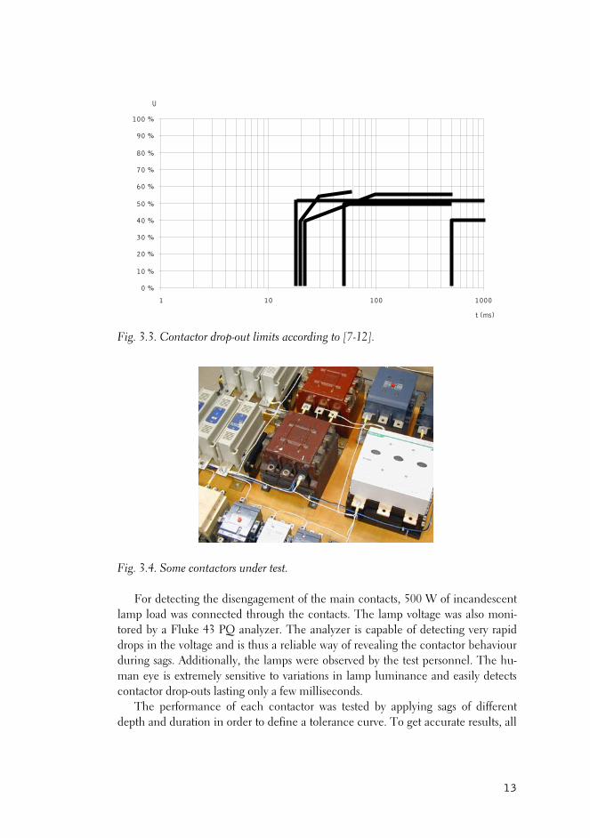
To provide additional results for comparison, contactors were also tested in the PQ (power quality) laboratory, as described in Ch. 3.1. The performance of 28 contactors rated from 9 to 900 A continuous current (AC-3) from 5 manufacturers was examined thoroughly. Some units were brand new while others had been in operation for several years. Some of the tested devices are shown in Fig. 3.4.
Few elderly contactors were rated at 220 V control voltage whereas the new ones comply with the up-to-date European 230 V rating. However, all of them were tested at 230 V, 50 Hz. The experiment set-up is shown in Fig. 3.5.
12
0 %
10 %
20 %
30 %
40 %
50 %
60 %
70 %
80 %
90 %
100 %
1 10 100 1000
t (ms)
U
Fig. 3.3. Contactor drop-out limits according to [7-12].
Fig. 3.4. Some contactors under test. For detecting the disengagement of the main contacts, 500 W of incandescent
lamp load was connected through the contacts. The lamp voltage was also moni-tored by a Fluke 43 PQ analyzer. The analyzer is capable of detecting very rapid drops in the voltage and is thus a reliable way of revealing the contactor behaviour during sags. Additionally, the lamps were observed by the test personnel. The hu-man eye is extremely sensitive to variations in lamp luminance and easily detects contactor drop-outs lasting only a few milliseconds.
The performance of each contactor was tested by applying sags of different depth and duration in order to define a tolerance curve. To get accurate results, all
13
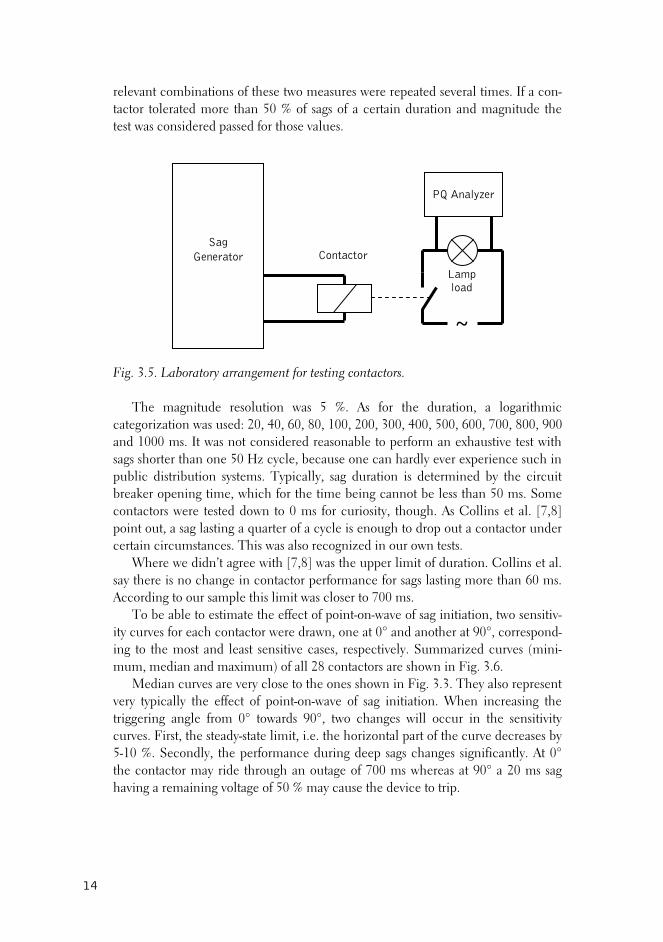
relevant combinations of these two measures were repeated several times. If a con-tactor tolerated more than 50 % of sags of a certain duration and magnitude the test was considered passed for those values.
PQ Analyzer
Fig. 3.5. Laboratory arrangement for testing contactors. The magnitude resolution was 5 %. As for the duration, a logarithmic
categorization was used: 20, 40, 60, 80, 100, 200, 300, 400, 500, 600, 700, 800, 900 and 1000 ms. It was not considered reasonable to perform an exhaustive test with sags shorter than one 50 Hz cycle, because one can hardly ever experience such in public distribution systems. Typically, sag duration is determined by the circuit breaker opening time, which for the time being cannot be less than 50 ms. Some contactors were tested down to 0 ms for curiosity, though. As Collins et al. [7,8] point out, a sag lasting a quarter of a cycle is enough to drop out a contactor under certain circumstances. This was also recognized in our own tests.
Where we didn’t agree with [7,8] was the upper limit of duration. Collins et al. say there is no change in contactor performance for sags lasting more than 60 ms. According to our sample this limit was closer to 700 ms.
To be able to estimate the effect of point-on-wave of sag initiation, two sensitiv-ity curves for each contactor were drawn, one at 0° and another at 90°, correspond-ing to the most and least sensitive cases, respectively. Summarized curves (mini-mum, median and maximum) of all 28 contactors are shown in Fig. 3.6.
Median curves are very close to the ones shown in Fig. 3.3. They also represent very typically the effect of point-on-wave of sag initiation. When increasing the triggering angle from 0° towards 90°, two changes will occur in the sensitivity curves. First, the steady-state limit, i.e. the horizontal part of the curve decreases by 5-10 %. Secondly, the performance during deep sags changes significantly. At 0° the contactor may ride through an outage of 700 ms whereas at 90° a 20 ms sag having a remaining voltage of 50 % may cause the device to trip.
Sag
Generator Contactor
Lamp load
~
14

In practice the duration of voltage sags is determined by the operating time of the medium voltage breaker and feeder relay. The combination of a processor based relay and an SF6 breaker is able to disconnect the faulted feeder in 50-70 ms. Sometimes an additional delay is allowed to prevent harmful outages. The delay seldom exceeds 500 ms. From the utility point of view the interesting range is thus from 50 to 500 ms. As can be seen in the median curves in Fig. 3.6, within this range the point-on-wave does not have much significance, neither does the dura-tion. The magnitude remains practically the only interesting measure and the most problematic 0° value gives a simple rule of thumb for contactor sag sensitivity. The distribution chart of this steady-state voltage limit for two point-on-wave angle val-ues (0° and 90°) in Fig. 3.7 shows the performance of the 28 tested contactors.
All values are between 20 % and 70 %, which also complies with the European standard [6]. Most tolerate 50 %, a commonly proposed level. Fig. 3.7 also clearly indicates that selecting a less sensitive contactor may drastically improve the overall sag sensitivity of the process.
0 %
10 %
20 %
30 %
40 %
50 %
60 %
70 %
80 %
90 %
100 %
10 100 1000
0° min 0° med 0° max
90° min 90° med 90° max
t (ms)
Fig. 3.6. Acquired voltage tolerance curves for 28 contactors. Note: Sags shorter than 20 ms were not included in the test.
15

0
2
4
6
8
10
12
0 % 10 % 20 % 30 % 40 % 50 % 60 % 70 % 80 % 90 % 100 %
0°
90°
Normal distribution
Nr. of contactors
Remaining voltage
Fig. 3.7. Acquired distribution of steady-state drop-out voltage for 28 contactors at two point-on-wave values. The normal distribution curve is also drawn.
16
3.1.2 Gas discharge lamps
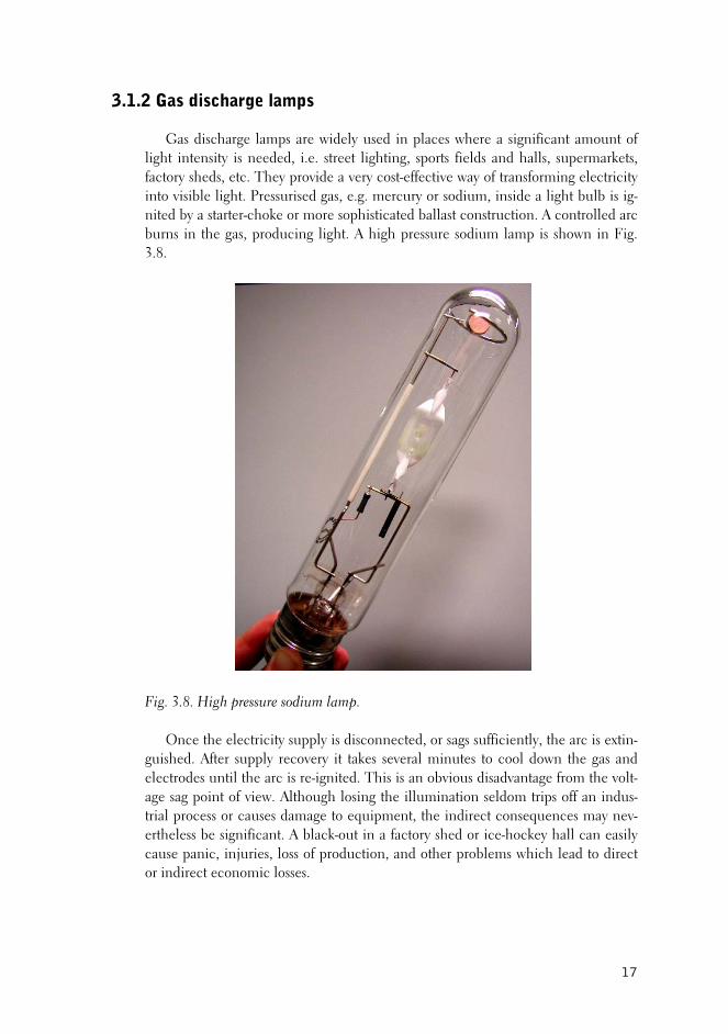
Gas discharge lamps are widely used in places where a significant amount of light intensity is needed, i.e. street lighting, sports fields and halls, supermarkets, factory sheds, etc. They provide a very cost-effective way of transforming electricity into visible light. Pressurised gas, e.g. mercury or sodium, inside a light bulb is ig-nited by a starter-choke or more sophisticated ballast construction. A controlled arc burns in the gas, producing light. A high pressure sodium lamp is shown in Fig.
Fig. 3
3.8.
.8. High pressure sodium lamp.
nce the electricity supply is disconnected, or sags sufficiently, the arc is extin-gui
Oshed. After supply recovery it takes several minutes to cool down the gas and
electrodes until the arc is re-ignited. This is an obvious disadvantage from the volt-age sag point of view. Although losing the illumination seldom trips off an indus-trial process or causes damage to equipment, the indirect consequences may nev-ertheless be significant. A black-out in a factory shed or ice-hockey hall can easily cause panic, injuries, loss of production, and other problems which lead to direct or indirect economic losses.
17

Standards for lamp, ballast and igniter manufacturers give no limits for the sys-tem performance during sags [13-18]. Some reference can be obtained, however. Testing limits for the rated performance of a luminaire are in most cases set to 92 % … 110 % of the nominal voltage. In other words, the system has to fulfil the manufacturer specifications at a steady-state voltage level of 92 % of the nominal. The minimum voltage level for stable operation of a lamp is typically 85-90 % of nominal. Above this level the starters and igniters may not cause any interference to the lamp. As one could assume from these figures, gas discharge lamps are very sensitive to voltage sag magnitude. There is no energy storage in the system as in the case of contactors and this makes the lamps sensitive to short duration sags as well.
Some studies on the topic have been carried out abroad [19-20]. Reference values for critical sag magnitude vary from 50 % to 80 % of nominal, most typical figures being closer to the upper value. A sag as short as a 0,5 cycle, at the specified magnitude may cause the lamp to extinguish. According to Dorr & al., lamp sensi-tivity to sags depends very much on the age of the lamp. The older the lamp, the more sensitive it is to voltage sags.
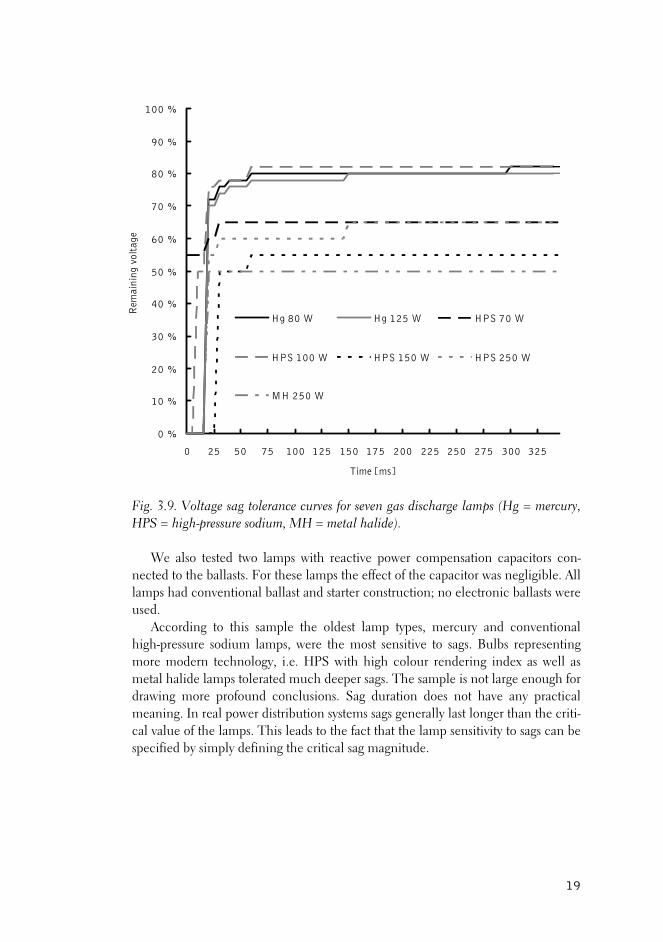
In our own tests, 7 gas discharge lamps of different brand, type and power rat-ing were tested. The sample included the following 230 V bulbs:
- mercury 80 W - mercury 125 W - high-pressure sodium 70 W - high-pressure sodium 100 W - high-pressure sodium with red correction coating 150 W - high-pressure sodium with red correction coating 250 W - metal halide 250 W
All lamps were aged for 100 hours before being subjected to the test. Sags were
applied to lamps under normal and stable operating conditions, i.e. after a proper warm-up period. The sensitivity curves in Fig. 3.9 were obtained for the lamps specified above.
18
0 %
10 %
20 %
30 %
40 %
50 %
60 %
70 %
80 %
90 %
100 %
0 25 50 75 100 125 150 175 200 225 250 275 300 325
Time [ms]
Rem
aini
ng v
olta
ge
Hg 80 W Hg 125 W HPS 70 W
HPS 100 W HPS 150 W HPS 250 W
MH 250 W
Fig. 3.9. Voltage sag tolerance curves for seven gas discharge lamps (Hg = mercury, HPS = high-pressure sodium, MH = metal halide).
We also tested two lamps with reactive power compensation capacitors con-
nected to the ballasts. For these lamps the effect of the capacitor was negligible. All lamps had conventional ballast and starter construction; no electronic ballasts were used.
According to this sample the oldest lamp types, mercury and conventional high-pressure sodium lamps, were the most sensitive to sags. Bulbs representing more modern technology, i.e. HPS with high colour rendering index as well as metal halide lamps tolerated much deeper sags. The sample is not large enough for drawing more profound conclusions. Sag duration does not have any practical meaning. In real power distribution systems sags generally last longer than the criti-cal value of the lamps. This leads to the fact that the lamp sensitivity to sags can be specified by simply defining the critical sag magnitude.
19
3.1.3 Microprocessor based equipment
Microprocessors are basic components in almost all types of electronics, from household appliances to complicated industrial process control devices. Personal computers (PC) and programmable logic controllers (PLC) are typical examples.
Common to this equipment category is the obvious sensitivity to supply under-voltage conditions. Low voltage electronics are usually powered by an ac/dc con-verter consisting of a conventional transformer-rectifier topology or a more sophis-ticated chopper construction. Capacitors are used on the dc side for filtering the ripple. In addition, the fully charged capacitor bank also contains a certain amount of energy that can be used for supply backup purposes in the case of a momentary input voltage drop. The rating of the capacitor determines the maximum depth and duration of a sag that can be successfully mitigated.
An unintended restart or lock-up of a processor based device may lead to vari-ous problems, ranging from loss of data to a shutdown or halt of a complete indus-trial process.
No standards have been established on the issue, probably due to the wide, het-erogeneous range of devices and solutions in this category. Instead, a common agreement by the manufacturers does exist. The so called ITI curve is published by the Information Technology Industry Council (ITI) [21]. The latest version is shown in Fig. 3.10. The previous version of the curve was known as CBEMA, which stands for Computer and Business Equipment Manufacturers Association.
Below the lower ITI curve there is a region where the loss of energy in the dc capacitor may cause unwanted operation or malfunction of the sensitive equip-ment. Permanent damage is anticipated under conditions violating the overvoltage limit curve but this seldom happens within the undervoltage region.
Because of the almost endless variety of device constructions and power supply units it is impossible to give precise limits for this kind of equipment. For example, the sensitivity of a computer is strongly dependent on the components and their operational state. Adding auxiliary devices and performing complex calculations require more power and further decrease the system sag tolerance. Sometimes PCs or logic controllers are supplied through a UPS backup, which increases their tol-erance significantly. It is possible, however, to acquire accurate results for a par-ticular device by performing exhaustive sag tests.
Some ride-through values for personal computers are presented in [20] by Brauner & al. The critical remaining voltage varies between 30 % and 65 % of nominal. The allowed duration of a total interruption ranges from 80 ms to 450 ms.
In our tests seven personal computers aged from 0 to 7 years were subjected to sags. Sags were made deeper and longer until the tested computer rebooted. The monitors were connected to another supply to prevent their effect on the behaviour of the central processing units. Results obtained for the test set are shown in Fig. 3.11.
20
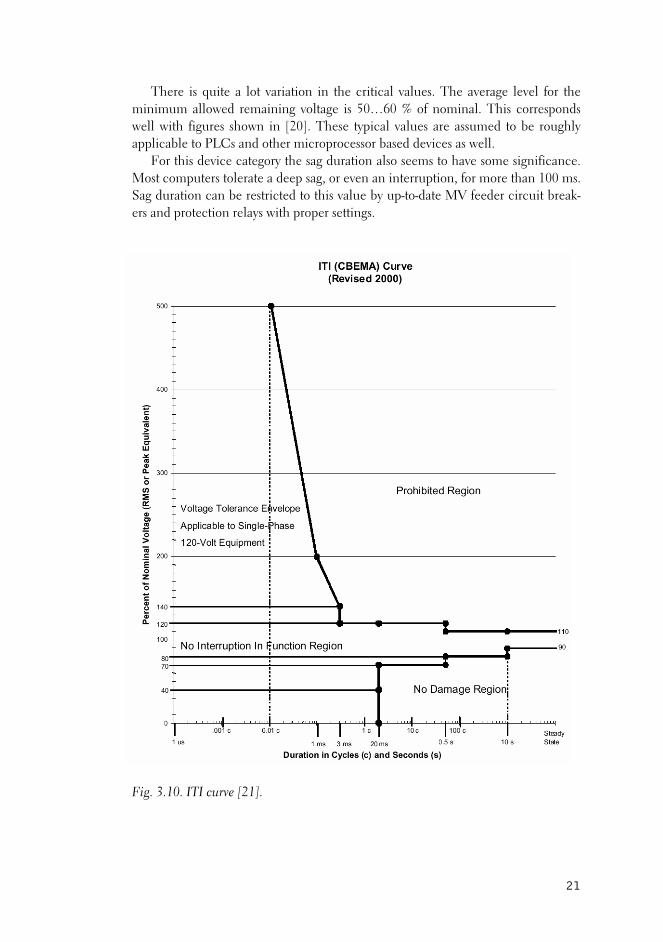
There is quite a lot variation in the critical values. The average level for the minimum allowed remaining voltage is 50…60 % of nominal. This corresponds well with figures shown in [20]. These typical values are assumed to be roughly applicable to PLCs and other microprocessor based devices as well.
For this device category the sag duration also seems to have some significance. Most computers tolerate a deep sag, or even an interruption, for more than 100 ms. Sag duration can be restricted to this value by up-to-date MV feeder circuit break-ers and protection relays with proper settings.
Fig. 3.10. ITI curve [21].
21

0 %
10 %
20 %
30 %
40 %
50 %
60 %
70 %
80 %
90 %
100 %
0 50 100 150 200 250 300 350 400 450 500 550 600
Time [ms]
Rem
aini
ng v
olta
ge
ITIC A-96 B-97 C-97
D-98 E-98 F-02 G-02
Fig. 3.11. Test results for seven computers. ITI curve is also shown. The numbers in-dicate the approximate year of manufacture.
3.1.4 Converters
Another group to be mentioned regarding voltage sag sensitivity comprises ac/ac- and ac/dc-converters. Variable speed drives are used to control motors in in-dustrial processes, building automation, water supply and sewerage, etc. Regardless of the converter construction there is always a dc link downstream from the ac in-put. Here also a capacitor is used to filter the dc ripple.
Compared to computer power supplies, converters are rated for a much higher output power. The capacitor is not rated accordingly and can thus not be used for backup supply purposes. In addition, it is not recommended to supply motors with sagged or unbalanced voltage. This is due to the risk of overheating and permanent damage to the equipment.
Converter control schemes are usually designed so that the undervoltage pro-tection trips the drive output as soon as the voltage drops down to the rated mini-mum operation voltage of the load. This not only protects the (motor) load from damage but also prohibits unwanted current increase on the converter input side.
These aspects lead us to the conclusion that there are two limits governing con-verter sag sensitivity:
- hardware limit determined by the dc link capacitor and the converter
load rate - software limit determined by the minimum load input voltage limit and
set by the user
22
If the software limit, i.e. undervoltage protection, is disengaged, the hardware limit applies. At the hardware limit the converter is not capable of providing rated performance but instead produces a sagged output voltage. How much the output voltage decreases depends on the component rating and load rate. Converter input unbalance is corrected in most cases, however.
As with computers, here also the variety of brands, constructions and power rat-ings is huge. It is neither possible nor reasonable to test all equipment on the mar-ket. Some estimates of typical values may be used or tests performed on devices of particular interest.
Existing standards for manufacturers give some guidelines, which are useful for determining the average values [22-27]. Most of them only give limits for the steady state input voltage. One limit is for uninterrupted operation, typically 90…110 % of nominal. Another, more strict, is the limit for rated performance, set to as high as 100…110 % of nominal in [24].
The IEC standard [25] for power drive system electromagnetic compatibility (EMC) issues superficially mentions sags of 70 % to 50 % remaining voltage and 300-1000 ms as problematic.
The standard for line commutated converters [27] establishes three immunity classes: a, b and c, which apply to both steady state and voltage events (0,5 to 30 cycles). Class a is the most tolerant and c the most sensitive. For steady state condi-tions the minimum is 95 % to 90 % of nominal depending on the immunity class. Violating this limit leads to “loss of performance”. For undervoltage events the minimum varies from 92,5 % to 85 % of nominal depending on the immunity class and whether the converter is used as an inverter or is intended for rectifier operation only. Voltage sags deeper than the given limits lead to “interruption of service due to protective devices”.
As can be seen, all these limits are very strict. The supply voltage should never go below 85 % of nominal even for a few milliseconds. As discussed above, this is mostly for protecting the load from permanent damage. When the software limit is set to 90 % or 85 % for this reason, it is not economically viable to make the hard-ware much more tolerant either.
Some motors in some applications operate without problems at undervoltage as well, whereas in others the momentary loss of torque or speed may be fatal to the process or equipment [28]. In the former cases the software limit can be set far be-low the standard recommendations or completely disengaged. Hardware then de-termines the ultimate trip-out voltage. From the point of view of the complete process it is extremely important to study whether running the motor below nomi-nal ratings will still adversely affect the process. For example, even though a vac-uum pump in a silicon wafer oven seems to run adequately at undervoltage the slight diminution of vacuum during a sag may completely spoil the product. It is thus totally dependent on the process whether running in this “grey zone” will or will not cause problems. Fig. 3.12 concludes the issue.
23
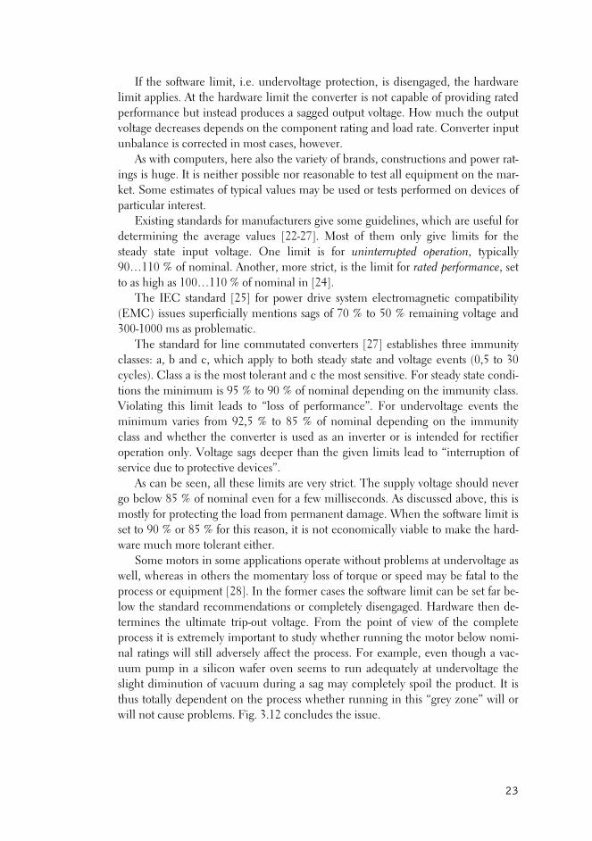
An optimal (and obvious) protection scheme should thus provide optimal pro-tection for the process, not only for the converter load device. A more sophisticated way is, instead of only concentrating on the protection scheme, to switch to a com-pletely different load control scheme while a sag is present. This alternative opera-tion mode is carefully and individually designed for each particular load to opti-mise the ride-through capabilities and process stability. An example is given in [29].
Fig. 3.12. Converter sag sensitivity. Software limit (shutdown by undervoltage protec-
terms of actual test results, Koch et al. gave minimum and maximum sag sen
100 %
85 % Uninterrupted performance Rated performance
SFS-EN 50160
HARDWARE LIMIT ZONEConverter disconnects
SOFTWARE LIMIT ZONE Effects d processepend on
Rem
aini
ng v
olta
ge
Duration
tion) can be freely set to any magnitude and duration outside the hardware limit zone.
Insitivity values for tested variable speed drives (VSD) [9]. The minimum voltage
amplitude ranges from 90 % to 60 % of nominal and the maximum duration of an outage varies between 50 and 500 milliseconds. IEEE Standard 1346-1998 [12] gives very similar example values, while pointing out that the figures should not be considered to represent typical performance.
24
3.2 Economic aspects
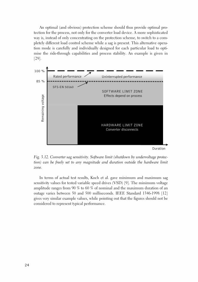
Why are we basically interested in voltage sags? The presence of sags in a power system introduces the risk of process interruption and further significant economic losses.
Before assessing the cost it is worth devoting some time to its source. We have two quantities that affect the cost: process sensitivity and sag frequency. Expressed as a probability distribution:
Process sensitivity Sag frequency
Pro
cess
tri
ppin
g pr
obab
ility
Nr.
of
sags
per
yea
r
Nr. of interruptions
Remaining voltage
Fig. 3.13. Probability of process interruption due to voltage sags.
Let the remaining voltage be u, process sensitivity P(u) and sag frequency S(u).
The risk of interruption is thus
S(u)P(u)I(u) ⋅= (3.1)
For this continuous distribution, the total number of sag related interruptions is written as:
(∫∫==
⋅==100%
0%u
100%
0%u
duS(u)P(u)I(u)duN ) (3.2)
Usually sag duration is also considered. In terms of Fig. 3.13 this leads to the addition of one more dimension. The three probability curves, I, P and S, are no longer curves but planes comprising u/t coordinates. Equation 3.2 also needs to be rewritten:
25
( ) dtdut)S(u,t)P(u,dtdut)I(u,Ntmax
0t
100%
0%u
tmax
0t
100%
0%u∫ ∫∫ ∫= == =
⎟⎟⎠
⎞⎜⎜⎝
⎛⋅=⎟⎟
⎠
⎞⎜⎜⎝
⎛= (3.3)
An unintended process shutdown means a lot of unexpected work, regardless of the cause of the interruption. Torn web on a paper mill production line or lost vac-uum in a silicon wafer oven may cost huge amounts of money. The line has to be shut down, cleaned and started up again. Loss of production and raw materials, delayed delivery penalties as well as paying the workers for overtime introduce ad-ditional costs. Ref. [12] proposes one thorough method for retrieving proper figures for the event cost of a sag related interruption.
Total cost may be assessed for one process or customer, customer category or for the customers of a complete power distribution company, depending on the standpoint. The more accurate the results required, the more focused the study should be.
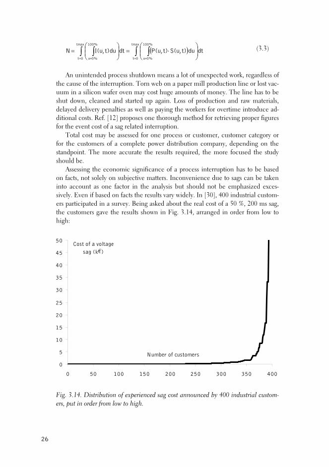
Assessing the economic significance of a process interruption has to be based on facts, not solely on subjective matters. Inconvenience due to sags can be taken into account as one factor in the analysis but should not be emphasized exces-sively. Even if based on facts the results vary widely. In [30], 400 industrial custom-ers participated in a survey. Being asked about the real cost of a 50 %, 200 ms sag, the customers gave the results shown in Fig. 3.14, arranged in order from low to high:
0
5
10
15
20
25
30
35
40
45
50
0 50 100 150 200 250 300 350 400
Number of customers
Cost of a voltage sag (k€)
Fig. 3.14. Distribution of experienced sag cost announced by 400 industrial custom-ers, put in order from low to high.
26
Although this is only one example, it is strongly assumed that it represents a
quite typical distribution. The curve shows that 150 of those 400 customers did not have any inconvenience or losses due to voltage sags whereas 2 %, i.e. less than 10 customers, accounted for 50 % of the total cost spanned by the curve. Obviously certain types of industry are more sensitive to power system disturbances than oth-ers. The chip manufacturing and process industries are often mentioned to be the most vulnerable. When the economic significance is high, more sophisticated methods for correcting the problems may also prove to be cost-effective.
The fact is that a vast amount of money is spent yearly for the consequences of voltage sags. A paper by the author et al. [31] gives an estimate for the total voltage sag related cost for the customers of five Finnish power distribution companies. Numbers range from 0,6 to 14,5 million € per company.
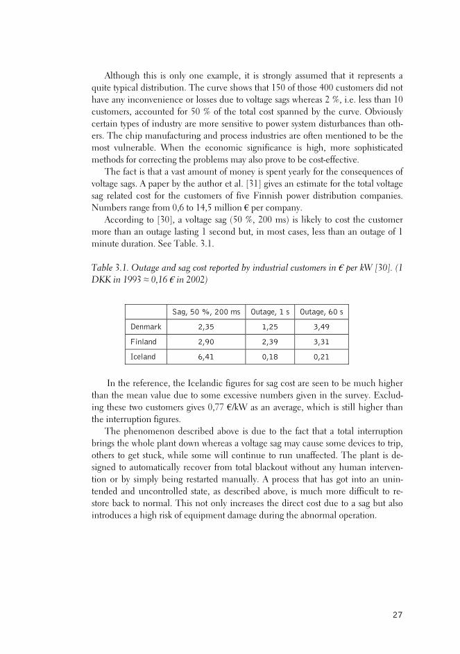
According to [30], a voltage sag (50 %, 200 ms) is likely to cost the customer more than an outage lasting 1 second but, in most cases, less than an outage of 1 minute duration. See Table. 3.1.
Table 3.1. Outage and sag cost reported by industrial customers in € per kW [30]. (1 DKK in 1993 ≈ 0,16 € in 2002)
Sag, 50 %, 200 ms Outage, 1 s Outage, 60 s
Denmark 2,35 1,25 3,49
Finland 2,90 2,39 3,31
Iceland 6,41 0,18 0,21
In the reference, the Icelandic figures for sag cost are seen to be much higher
than the mean value due to some excessive numbers given in the survey. Exclud-ing these two customers gives 0,77 €/kW as an average, which is still higher than the interruption figures.
The phenomenon described above is due to the fact that a total interruption brings the whole plant down whereas a voltage sag may cause some devices to trip, others to get stuck, while some will continue to run unaffected. The plant is de-signed to automatically recover from total blackout without any human interven-tion or by simply being restarted manually. A process that has got into an unin-tended and uncontrolled state, as described above, is much more difficult to re-store back to normal. This not only increases the direct cost due to a sag but also introduces a high risk of equipment damage during the abnormal operation.
27

4 MITIGATION OF VOLTAGE SAGS
As voltage sags are a recognised power quality issue and a source of significant economic losses, various means for mitigating the consequences of sags have been developed. Basically, all these solutions aim to reduce the number and severity of
Fig. 4.1. Probabilistic risk of process interruption when mitigation is used. Dotted
sags experienced by a sensitive customer. See Fig. 4.1 and compare with Fig. 3.13.
ne solution is to use conventional means and regular power system compo-nen
4.1 Custom power technology
A more sophisticated way, although no longer so novel or emerging, is called cus
fers to premium power quality customized to meet the cus
Process sensitivity Original sag frequency
lines represent the original sag frequency and interruption risk curves. Ots to prevent faults or restrict the penetration of sags in a network. Tree trim-
ming, surge protection, load rearrangement and separation of sensitive loads are well-known and widely used examples.
tom power technology. The expression “custom power” was established by Dr. Narain G. Hingorani in 1988 [32]. In the reference he writes about custom power: The term describes the value-added power that electric utilities and other service pro-viders will offer their customers and …a prominent feature will be the application of power electronic controllers.
“Custom power” thus retomers’ needs. Further, the term “custom power technology” describes the
equipment used for providing custom power. The technology is based on power
Pro
cess
tri
pppi
ng p
roba
bilit
y
Remaining voltage
Mitigated sag frequency
Nr. of interruptions
Nr.
of
sags
per
yea
r
28
electronics and also, on some occasions, electrical energy storage. Below the ab-breviation CP stands for custom power.
Custom power technology is a general term for equipment capable of mitigat-ing
g voltage sags, i.e. protecting a sensitive load from network distur-ban
- switching the load to another supply rgy storage
rrent (booster)
he first is simply a rapid transfer switch, capable of switching the load to an-oth
ergy storage, for inject-ing
gy available, the inverter injects energy dra
discuss the characteristics of existing custom power sag mi
4.1.1 Transfer switch
The solid-state transfer switch, also referred to as a sub-cycle or static transfer swi
numerous power quality problems including voltage sags. Basic functions are fast switching and current or voltage injection for correcting anomalies in supply voltage or load current. Injecting or absorbing both active and reactive power is possible. Current injection is typically used for protecting the power system from a polluting load.
For mitigatinces, there are three basic custom power applications:
- injecting missing voltage from an ene- injecting missing voltage by increasing the line cu
Ter supply. The more independent this alternative supply is from the primary
supply, the higher level the load voltage can be restored to. The second option utilizes an inverter, equipped with en the missing voltage. After supply voltage recovery the storage is recharged to
full capacity for upcoming challenges. The size of the storage determines the maxi-mum duration of sag that can be restored.
In a case where there is no stored enerwn from the sagged supply, in other words converts current on the supply side
into voltage on the load side. This construction requires some voltage to remain in the supplying power system in order to perform the conversion. Deep sags and out-ages are beyond its reach.
The following chapterstigation applications and the corresponding power system requirements in de-
tail. Rather than giving exact brand-related figures the scope is on general perform-ance and modelling of mitigation capabilities.
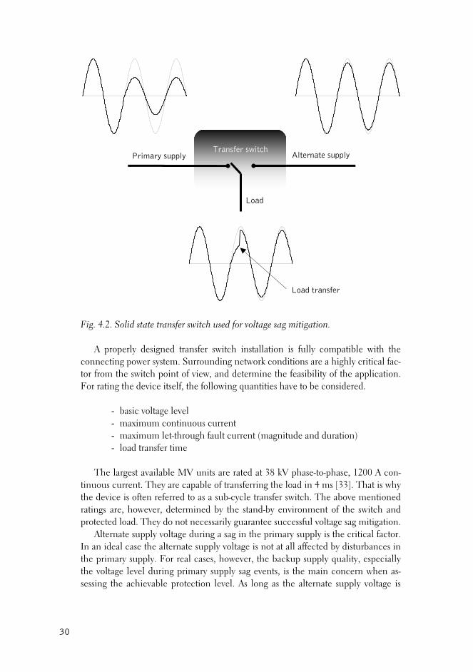
tch, is already an off-the-shelf product. The switch simply connects sensitive load(s) to an alternate supply as soon as a sag is registered in the primary supply. See Fig. 4.2.
29
Transfer switch
Primary supply Alternate supply
Load
Load transfer
Fig. 4.2. Solid state transfer switch used for voltage sag mitigation. A properly designed transfer switch installation is fully compatible with the
connecting power system. Surrounding network conditions are a highly critical fac-tor from the switch point of view, and determine the feasibility of the application. For rating the device itself, the following quantities have to be considered.
- basic voltage level - maximum continuous current - maximum let-through fault current (magnitude and duration) - load transfer time
The largest available MV units are rated at 38 kV phase-to-phase, 1200 A con-
tinuous current. They are capable of transferring the load in 4 ms [33]. That is why the device is often referred to as a sub-cycle transfer switch. The above mentioned ratings are, however, determined by the stand-by environment of the switch and protected load. They do not necessarily guarantee successful voltage sag mitigation.
Alternate supply voltage during a sag in the primary supply is the critical factor. In an ideal case the alternate supply voltage is not at all affected by disturbances in the primary supply. For real cases, however, the backup supply quality, especially the voltage level during primary supply sag events, is the main concern when as-sessing the achievable protection level. As long as the alternate supply voltage is
30

acceptable there is no time limit for this mitigation technique, which is a major advantage.
An alternate MV supply may be arranged in many ways. In areas where the HV transmission system is strong enough and substations are equipped with more than one HV/MV transformer, it may be adequate to transfer the sensitive load(s) from one transformer to another. See Fig. 4.3.
HV/MV transformers
MV feeders
MV busbars
SSTS
Sag sensitive loadFault
Fig. 4.3. Solid-state transfer switch at an HV/MV substation. Primary and alternate supplies are taken from different transformers.
The cause of the sag is in this case assumed to be a fault on one of the MV
feeders. The following discussion also applies to other origins of voltage sags, how-ever. The schematic diagram of the arrangement is shown in Fig. 4.4.
The load voltage during the voltage sag is in this case written:
SOURCESTMF
TMFPCCLOAD U
ZZZZZZZ
UU ⋅+++
++== (4.1)
Let us calculate an example. For achieving the most severe case we assume a zero-impedance 3-phase fault occurs at the substation MV busbar, i.e. ZF = 0 and ZM = 0. Thus the load voltage after the switching operation, and the obtained pro-tection level, is dependent on the transformer and source impedances only:
31

SOURCEST
TPCCLOAD U
ZZZ
UU ⋅+
== (4.2)
In practice these impedances refer to the HV system short circuit capacity and HV/MV transformer rating. See Fig. 4.5. The transformer short circuit reactance zk is here assumed to be 10 % for ratings up to 30 MVA, and 12 % for transformers rated at 40 MVA and higher. According to the figure, for example, an 80 % protec-tion level is achieved by using a 25 MVA 110/21 kV transformer in systems where the HV short circuit current is 5 kA or more.
SourceU
SOURCE
Transformer Z
T
MV feeder Z
M
Fault Z
F
SSTS Fault current
Source Z
S
UBUS
UPCC
Transformer
Pro
tect
ed
feed
er
Fau
lted
fe
eder
Fig. 4.4. Schematic diagram where the transfer switch is connected to two separate transformers located at the same substation.
32

0
5
10
15
20
25
30
10 20 30 40 50 60 70
110/21 kV transformer rating (MVA)
Sho
rt c
ircu
it c
urre
nt a
t 1
10
kV
(kA
)
90 % 80 %
70 % 60 %
Fig. 4.5. Obtained protection level, i.e. the minimum voltage at load terminals as a function of short circuit current and transformer rating.
At distant substation or plant sites it may be necessary to build an MV feeder
from another substation. In such a case the point of common coupling (PCC) is located higher upstream in the grid. See Fig. 4.6.
In a simplified case where both supplying HV subsystems are radial, i.e. there are no closed HV loops downstream the PCC, the remaining load voltage after supply transfer is written:
SOURCESHTMF
HTMFPCCLOAD U
ZZZZZZZZZ
UU ⋅++++
+++== (4.3)
Again, if we want to create a worst case scenario, a 3-phase fault is assumed at the substation MV busbar. Thus
SOURCESHT
HTPCCLOAD U
ZZZZZ
UU ⋅++
+== (4.4)
If the supplying HV systems include closed loops, more complicated calcula-tions must be performed, though. Disregarding the network structure and required method of calculation, the quantities to consider seem to be: the transformer rat-ing, HV line type and length, connection between the transformers and PCC as well as the short circuit current at the PCC.
33

Source at PCC Z
S
Source U
SOURCE
HV line Z
H
Transformer Z
T
MV feeder Z
M
Fault Z
F
SSTS Fault current
UBUS
UPCC
Transformer
MV line
Pro
tect
ed
feed
er
Fau
lted
fe
eder
Fig. 4.6. Schematic diagram for the case where the alternate supply for the transfer switch is taken from another substation through an MV backup feeder.
In Fig. 4.7 some example numbers are calculated for a 110/21 kV system and a
25 MVA transformer. The HV conductor reactance is assumed to be 0,4 ohm/km and the lines are assumed to be connected radially from the PCC to the HV/MV transformers.
According to this calculation, the PCC short circuit current has much more relevance than the HV line length. Obtaining a high protection level requires a rather high short circuit current rating, i.e. a strong HV system.
34

0
2
4
6
8
10
12
14
0 10 20 30 40 5
110 kV line length between transformer and PCC (km)
Sho
rt c
ircu
it c
urre
nt a
t P
CC
(kA
)
90 % 80 %
70 % 60 %
0
Fig. 4.7. Achieved protection level for a 25 MVA transformer as a function of PCC short circuit current and HV line length between the transformer and PCC.
4.1.2 Series power conditioner with energy storage
In cases where the transmission system is weak or a back-up supply neither ex-ists nor is reasonable to build, a transfer switch does not necessarily provide suffi-cient protection against voltage sags. Something else has to be considered.
For correcting a sagged public supply, another voltage source, connected in se-ries with the troubled one, is needed at the sensitive load. In a successfully rated system these two sources together add up to sufficient load voltage, although not necessarily 100 %.
Unlike the case of a transfer switch, the network environment is not as critical as the correct rating and compatibility with the connected load. Sufficient mitiga-tion is usually achievable in weak power systems as well.
This technology is also available commercially. Due to the variety of brands and models, it is neither possible nor reasonable to give detailed information of their features within this publication. Some general facts about rating and per-formance are discussed to serve the purpose of this thesis, though.
Probably the best known name for such an application is the dynamic voltage restorer, DVR. Despite the name, all solutions consist of an inverter and a trans-former used for interconnection. Injected active power is taken from a dc energy storage. The basic construction of a series connected power conditioner is shown in Fig. 4.8.
The dc energy storage is charged through a rectifier. When a sag occurs, the inverter injects a current that flows through the transformer, whose secondary winding is connected in series with the supply feeder. The transformer winding ra-
35
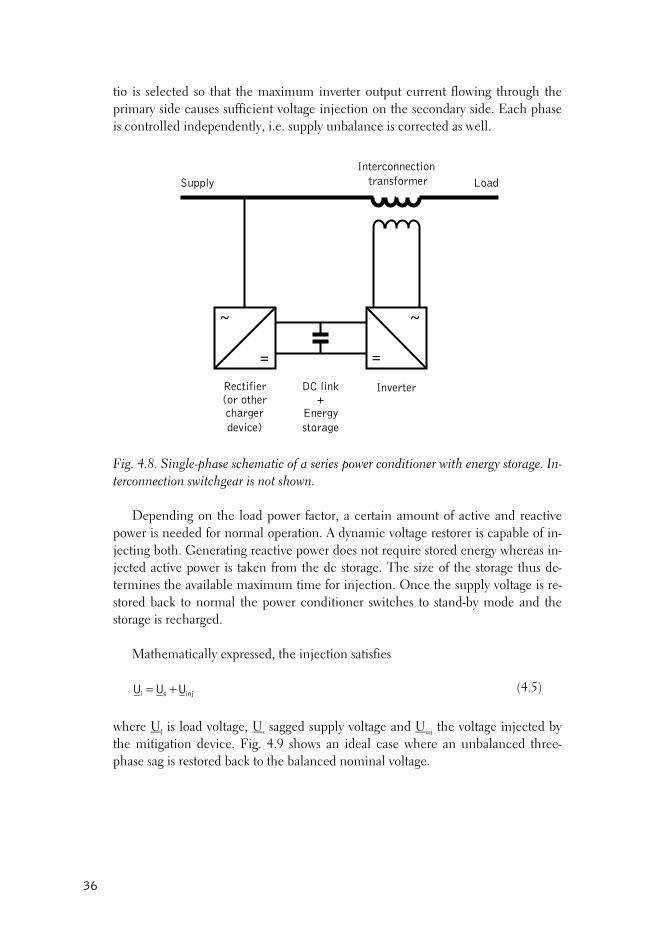
tio is selected so that the maximum inverter output current flowing through the primary side causes sufficient voltage injection on the secondary side. Each phase is controlled independently, i.e. supply unbalance is corrected as well.
Interconnection transformer
Fig. 4.8. Single-phase schematic of a series power conditioner with energy storage. In-terconnection switchgear is not shown.
Depending on the load power factor, a certain amount of active and reactive
power is needed for normal operation. A dynamic voltage restorer is capable of in-jecting both. Generating reactive power does not require stored energy whereas in-jected active power is taken from the dc storage. The size of the storage thus de-termines the available maximum time for injection. Once the supply voltage is re-stored back to normal the power conditioner switches to stand-by mode and the storage is recharged.
Mathematically expressed, the injection satisfies
injsl UUU += (4.5)
where Ul is load voltage, Us sagged supply voltage and Uinj the voltage injected by the mitigation device. Fig. 4.9 shows an ideal case where an unbalanced three-phase sag is restored back to the balanced nominal voltage.
DC link +
Energy storage
~
=
Supply Load
~
=Rectifier Inverter (or other charger device)
36
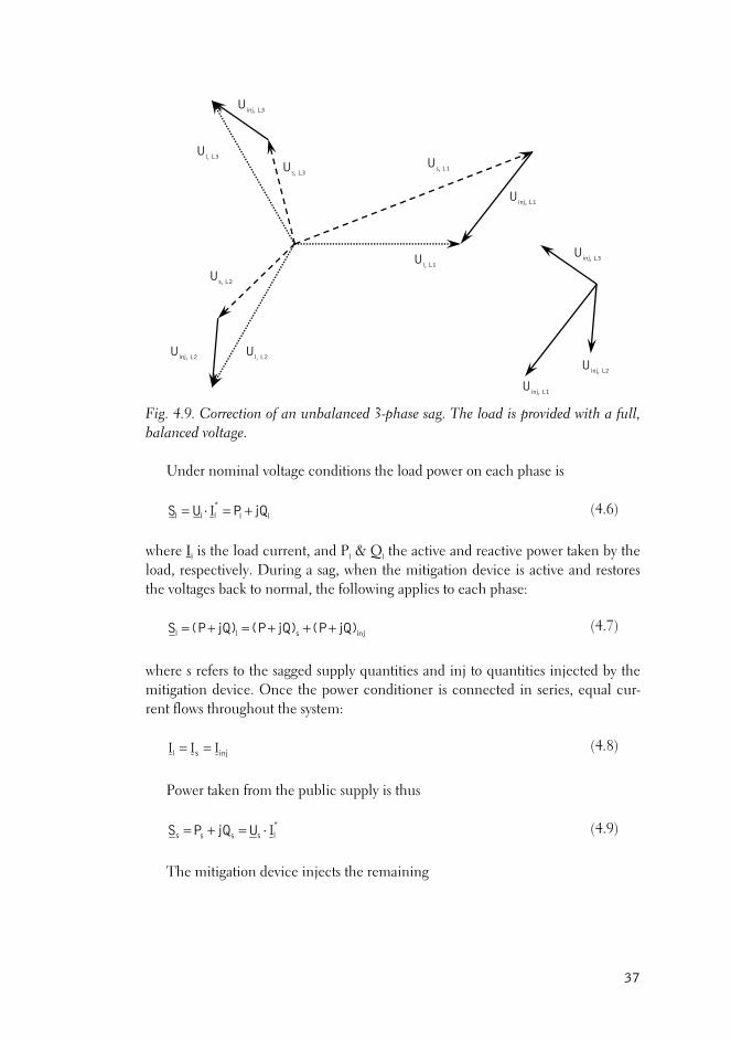
Fig. 4.9. Correction of an unbalanced 3-phase sag. The load is provided with a full, balanced voltage.
Under nominal voltage conditions the load power on each phase is
ll*lll jQPIUS +=⋅= (4.6)
where Il is the load current, and Pl & Ql the active and reactive power taken by the load, respectively. During a sag, when the mitigation device is active and restores the voltages back to normal, the following applies to each phase:
injsll jQ)(PjQ)(PjQ)(PS +++=+= (4.7)
where s refers to the sagged supply quantities and inj to quantities injected by the mitigation device. Once the power conditioner is connected in series, equal cur-rent flows throughout the system:
injsl III == (4.8)
Power taken from the public supply is thus
*lssss IUjQPS ⋅=+= (4.9)
The mitigation device injects the remaining
Uinj, L1
Uinj, L2
Uinj, L3U
l, L1
Ul, L3
Ul, L2
Us, L1
Us, L2
Us, L3
Uinj, L3
Uinj, L1
Uinj, L2
37

⎩⎨⎧
−=
−=
slinj
slinj
QQQ
PPP (4.10)
where Qinj is generated by the inverter and Pinj is taken from the energy storage, the total apparent power being
injinjinj jQPS += (4.11)
This maximum injection power is limited by the current rating of the inter-connection transformer windings and the inverter primary circuit. In addition, the energy storage size determines the maximum available active power as a function of time:
∫ ⋅=t
injinj dt(t)PE (4.12)
Typically, due to the unpredictable duration of sags, the device control scheme is set to limit the maximum voltage injection to a certain level, in order to provide the rated protection level for the rated time. In the case of a rectangular sag this makes the protected region rectangular when expressed in U/t coordinates. See Fig. 4.10.
This is a simplification, of course. If the sag is non-rectangular, the voltage in-jection is real-time controlled and adjusted to provide constant load voltage at the nominal or defined ride-through level but must not, however, exceed the maxi-mum voltage injection.
Fig. 4.10. Rating of a series power conditioner equipped with an energy storage.
Nominal voltage level (or plant ride-through level)U
n
Rem
aini
ng v
olta
ge
Time tcrit
injection max. magnitude
Uinj, max
PLANT SAVED PLANT LOST due to sag duration
max. durationfor U
inj, max
Ucrit
PLANT LOST PLANT LOST due to sag depth
due to sag depth and duration
38
In terms of Fig. 4.10 there are two major rating parameters for the device, Uinj,max, and tcrit. The maximum voltage injection of the inverter, Uinj,max, and the nominal (or plant ride-through) level Un determine the critical remaining voltage during a sag, Ucrit.
maxj,inncrit UUU −= (4.13)
Below Ucrit the plant cannot be saved, assuming Un is the minimum allowable load voltage, i.e. the plant ride-through level. The inverter may be able to give full injection even though the supply voltage drops below Ucrit. However, there typically exists a minimum input voltage limit for a series power conditioner, below which the device is disengaged. This limit is set to Ucrit or less depending on various rat-ing, protection and electric environment parameters.
The maximum time for full injection (Uinj,max) is tcrit. This is the maximum al-lowed sag duration in the case where the voltage sags down to Ucrit. These two pa-rameters, Uinj,max and tcrit, are related by the required active power and further by the amount of stored energy. See Eq. 4.12.
If the injected active power Pinj remains constant over the observed period of time, which seldom happens in reality, tcrit can be expressed mathematically in general form:
injcrit P
Et = (4.14)
The parameters discussed above are used for rating the device. In addition to the sags within the rated region discussed above, the power conditioner may also be capable of restoring sags lasting longer than tcrit. This is possible for sags less se-vere than Ucrit, providing the total available amount of active power is not exceeded. Eq. 4.15 thus has to be satisfied. See also Fig. 4.11.
maxinj,injcritmaxinj.inj UUtUtU ≤∀⋅≤⋅ (4.15)
where Uinj and t are the magnitude and duration of injection in this particular case and t > tcrit. The load current is considered to remain constant throughout the event. Further, Eq. 4.15 can be written
maxinj,injcritinj
maxinj, UUtU
Ut ≤∀⋅≤ (4.16)
In the region where U ≥ Ucrit and the sag duration t is longer than the limit de-termined by Eq. 4.16 the sags are shortened by tcrit. Depending on the process this may have a slight positive effect on the plant protection.
39

Nominal voltage level (or plant ride-through level)
Fig. 4.11. In a case where the remaining voltage is higher than Ucrit, the mitigation device may be capable of saving a plant against sags lasting longer than tcrit. The ac-cessible amount of stored energy is the limiting factor.
The features discussed above are typically left outside rating considerations but
may introduce some improvement in plant sag sensitivity as an additional benefit. In practice, however, an individual sag may vary in magnitude and therefore
this rectangular or curvilinear way of presentation is somewhat simplified. Never-theless, for preventive measures like device rating and cost/benefit analysis of the mitigation, this is a most reasonable way.
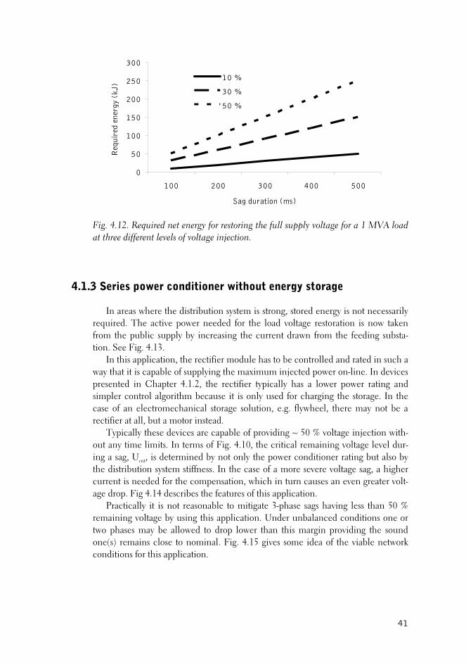
In addition to the already discussed rating parameters, Uinj,max and tcrit, there are some other quantities to consider. Total power rating (P and Q), basic insulation level and maximum let-through fault current are the most important. Physically, the multiplication of active power and time is expressed as the size of the energy storage in joules. In Fig. 4.12, the rating of a storage application is shown. No losses are considered.
The electric energy storage type has to be selected as well. Capacitors are per-haps the most used but batteries, flywheels and superconducting coils (SMES) have also been introduced. Some conventional switchgear is needed for by-pass and maintenance purposes.
Rem
aini
ng v
olta
ge
Time tcrit
Un
PLANT SAVED
Uinj,max
Sags shortened by tcrit
Ucrit
40
0
50
100
150
200
250
300
100 200 300 400 500
Sag duration (ms)
Req
uire
d en
ergy
(kJ
)
10 %
30 %
50 %
Fig. 4.12. Required net energy for restoring the full supply voltage for a 1 MVA load at three different levels of voltage injection.
4.1.3 Series power conditioner without energy storage
In areas where the distribution system is strong, stored energy is not necessarily required. The active power needed for the load voltage restoration is now taken from the public supply by increasing the current drawn from the feeding substa-tion. See Fig. 4.13.
In this application, the rectifier module has to be controlled and rated in such a way that it is capable of supplying the maximum injected power on-line. In devices presented in Chapter 4.1.2, the rectifier typically has a lower power rating and simpler control algorithm because it is only used for charging the storage. In the case of an electromechanical storage solution, e.g. flywheel, there may not be a rectifier at all, but a motor instead.
Typically these devices are capable of providing ~ 50 % voltage injection with-out any time limits. In terms of Fig. 4.10, the critical remaining voltage level dur-ing a sag, Ucrit, is determined by not only the power conditioner rating but also by the distribution system stiffness. In the case of a more severe voltage sag, a higher current is needed for the compensation, which in turn causes an even greater volt-age drop. Fig 4.14 describes the features of this application.
Practically it is not reasonable to mitigate 3-phase sags having less than 50 % remaining voltage by using this application. Under unbalanced conditions one or two phases may be allowed to drop lower than this margin providing the sound one(s) remains close to nominal. Fig. 4.15 gives some idea of the viable network conditions for this application.
41

Interconnection transformer
Fig. 4.13. Single phase schematics of a series power conditioner without energy stor-age. Interconnection switchgear is not shown. Rectifier is capable of supplying full power for the inverter on-line.
Fig. 4.14. Rating of a series power conditioner without stored energy.
~
=
Supply Load
~
=
Rectifier DC link Inverter
PLANT LOST due to sag depth
PLANT SAVEDinjection max.
magnitude U
inj, max
Nominal voltage level (or plant ride-through level)U
n
Rem
aini
ng v
olta
ge
Ucrit
Time
42
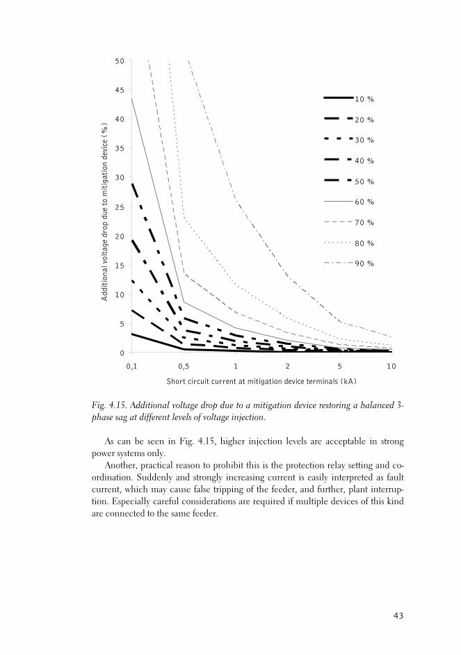
0
5
10
15
20
25
30
35
40
45
50
0,1 0,5 1 2 5 10
Short circuit current at mitigation device terminals (kA)
Add
itio
nal v
olta
ge d
rop
due
to m
itig
atio
n de
vice
(%
)10 %
20 %
30 %
40 %
50 %
60 %
70 %
80 %
90 %
Fig. 4.15. Additional voltage drop due to a mitigation device restoring a balanced 3-phase sag at different levels of voltage injection.
As can be seen in Fig. 4.15, higher injection levels are acceptable in strong
power systems only. Another, practical reason to prohibit this is the protection relay setting and co-
ordination. Suddenly and strongly increasing current is easily interpreted as fault current, which may cause false tripping of the feeder, and further, plant interrup-tion. Especially careful considerations are required if multiple devices of this kind are connected to the same feeder.
43

4.2 Other means of mitigation
In addition to the applications presented above, the solid-state transfer switch and the series connected power conditioners, there are other means to mitigate voltage sags.
The static tap changer, uninterruptible power supply (UPS) and constant volt-age transformer are capable of taking care of the voltage restoration as well. Be-cause they are, however, from the scope of this thesis very similar in performance, no detailed discussion is presented here. They can be modelled by using the same simplified parameters as for the devices in Chapters 4.1.1 - 4.1.3.
44

5 PROB-A-SAG METHOD
To optimise investments, minimize inconvenience and maximize process per-formance in environments where voltage sags are frequent, a careful and thorough analysis is required. Process sensitivity, annual sag frequency, sag related cost and the performance of eventual mitigation equipment are the figures and factors to be considered. The most challenging task is to find a common mode for presenting all these quantities, which are inherently very different from each other.
This chapter presents a novel analysis and optimization method named Prob-A-Sag (Probabilistic Arrays for voltage Sag management), which successfully com-bines the consequences, economic significance and mitigation of voltage sags in a uniquely flexible way, also applicable to computerized processing.
The fundamentals of applied mathematics can be found, for example, in Ref. [34].
5.1 Existing methods
IEEE standard 1346-1998 “IEEE recommended practice for evaluating electric power system compatibility with electronic process equipment” [12] recommends methodology for voltage sag analysis. Assessing the annual number of power qual-ity related disruptions and determining the process sag sensitivity are the main tasks presented. From the outcome of these two studies, a system designer or analyst should be able to evaluate the cost of compatibility between the process and power system as well as to find alternatives to correct the problems.
This application is very similar to high voltage insulation coordination. Differ-ent curves of device sensitivity and the annual sag distribution, i.e. the sag envi-ronment, are drawn and placed upon each other. Further, these coordination charts are studied, losses evaluated and the optimal solution proposed. See Fig. 5.1.
The method is illustrative and quickly gives an estimate of the prevailing situa-tion and potential problems. However, human thinking, consideration and inter-vention are needed throughout the procedure. Despite the illustrative nature of its presentation, using paper and pencil and observing the drawn curves with the hu-man eye do not comply with the requirements of an exact and up-to-date analysis method. Neither can it be used for computerized calculation.
The standard enables a rough and quick estimate of sag related problems in a power system but a thorough and precise numerical analysis for a larger industrial process is not possible. Another major disadvantage is that a probabilistic approach is not taken. Process sag sensitivity, especially in large, complicated processes, is always a probabilistic function of several variables, such as the sensitivity of a single device and its eventual random variation, as well as the device’s connection to other devices in the process. The more sag sensitive devices there are in a process, the more important it is to use probabilistic methodology.
45

Generally, the technical approach seems to be quite approximate whereas the analysis of the overall economic impact of a sag related plant disruption is per-formed in a very thorough way. Everything from idle labour to repair parts is calcu-lated. Finally, the payback time is obtained for the money invested in corrective
Fig. 5.1. Example of the
measures. See Fig. 5.2.
analysis procedure recommended by IEEE Std. 1346-1998
Fig. 5.2. IEEE Std 1346-1198. Calculation of pay back time [12, picture copied from 35].
[12, picture copied from 35].
46
This makes the procedure a good tool for business people but it is not necessar-ily accurate enough for power systems people. From the power systems point view, the emphasis should be on technical and electrical analysis as much as it ison financial matters. Economic figures can be provided by either the customer othe power system analyst whereas the thorough technical analysis needs some ex-pertise in engineering.
A search in the IEEE database reveals that most references to this standard seem to concern the device sensitivity curves, not the method itself. According tothe standard the curves are, however, intended only to be examples and not to rep-resent the typical performance of a device.
Objectives for novel method
The ambitious primary aim of this work was to develop a method for analysing
of
r
5.2
sed solution for a problem in any voltage sag concerned power system or process. The following conditions were to be met:
- all quantities should be presented in a uniform format - applicable to all environments from a single customer to a complete
power distribution system - flexible accuracy from a rough estimate to exact numbers - must allow for probabilistic processing of data - possibility to be implemented in power system software platforms - includes tools for investigating custom power applications and other
means of mitigation The uniform way of presenting all variables was chosen to be a 2-dimensional
array. All quantities needed for the analysis can be expressed as an array which has rows for remaining voltage magnitude and columns for the duration of the sag. An example is shown in Fig. 5.3.
the technical and economic impacts of voltage sags, including features for finding the optimi
47

< 100 %
< 90 %
< 80 %
< 70 %
< 60 %
< 50 %
< 40 %
< 30 %
< 20 %
Re
< 10 %
aini
ng v
olta
ge
m
0-50 ms 50-150 ms 150-300 ms 300-500 ms 500 ms-1s
Sag duration
Fig
<
. 5.3. Example of an array used for presenting the variables. Each quantity, e.g. a device sag sensitivity, is indicated by placing numbers (bi-
nary or decimal) in corresponding cells. See Fig. 5.4.
100 % 0 0 0 0 0
< 90 % 0 0 0 0 0
< 80 % 0 0 0 0 0
< 70 % 0 0 0 0 0
< 60 % 0 1 1 1 1
< 50 % 0 1 1 1 1
< 40 % 0 1 1 1 1
< 30 % 0 1 1 1 1
< 20 % 0 1 1 1 1
Rem
aini
ng v
olta
ge
< 10 % 0 1 1 1 1
0-50 ms 50-150 ms 150-300 ms 300-500 ms 500 ms-1s
Sag duration
Fig. 5.4. Example of a device sensitivity array. (Sag sensitivity of a personal com-puter, 0 = no trip, 1 = trip.)
The cells of an array are referred to in the same way as matrix entries: A(i,j),
where i is the row number and j identifies the column in matrix A. The uppermost cell on the left is A(1,1). An example is shown in Fig. 5.5. Each entry corresponds to a cell value in a 3 x 3 array.
48
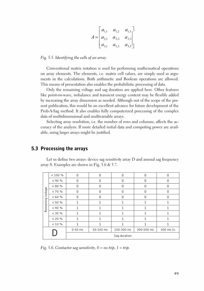
⎥⎥⎥
⎦
⎤
⎢⎢⎢
⎣
⎡=
3,32,31,3
3,22,21,2
3,12,11,1
aaaaaaaaa
A
Fig. 5.5 f an array.
Co matrix notation is used for performing mathon array elements. The elements, i.e. matrix cell values, are -ments calculations. Both arithmetic and Boolean operations are allowed. This means of pre also e p f d
Only the remaining voltage and sag du plied here. Other features like point-on-wave, imbalance and transient energy content may be flexibly added
pe of the pre-sent publication, this would be an excellent advance for future development of the Pro
electing array resolution, i.e. the number of rows and columns, affects the ac-curacy nalysi more detailed initial data and computing power are avail-able, using larger arra might be justified.
5.3 Processing the arrays
e e two ays: device sag sensitivity array D and annual sag frequency array S es are own in Fig .6 & 5.7.
. Identifying the cells o
nventional ematical operations simply used as argu
in the sentation enables th probabilistic rocessing o ata.
ration are ap
by increasing the array dimension as needed. Although out of the sco
b-A-Sag method. It also enables fully computerized processing of the complex data of multidimensional and multivariable arrays.
S of the a s. If
ys
L t us defin arr. Exampl sh . 5
< 100 % 0 0 0 0 0
< 90 % 0 0 0 0 0
< 80 % 0 0 0 0 0
< 70 % 0 0 0 0 0
< 60 % 0 0 0 0 0
< 50 % 1 1 1 1 1
< 40 % 1 1 1 1 1
< 30 % 1 1 1 1 1
< 20 % 1 1 1 1 1
Re
olta
ge
mai
ning
v
< 10 % 1 1 1 1 1
0-50 ms 50-150 ms 150-300 ms 300-500 ms 500 ms-1s D Sag duration
Fig. 5.6. Contactor sag sensitivity, 0 = no trip, 1 = trip.
49
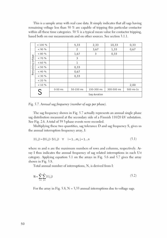
This is a sample array with real case data. It simply indicates that all sags having remaining voltage less than 50 % are capable of tripping this particular contactor within all these time categories. 50 % is a typical mean value for contactor tripping, based both on our measurements and on other sources. See section 3.1.1.
< 100 % 5,33 2,33 10,33 0,33
< 90 % 2 3,67 1,33 0,67
< 80 % 1,67 3 0,33
< 70 % 3
< 60 % 1
< 50 % 0,33
< 40 % 0,67
< 30 % 0,33
< 20 %
R
< 10 % 2,00
ege
m
aini
ng v
olta
0-50 ms 50-150 ms 150-300 ms 300-500 ms 500 ms-1s S Sag duration
Fig. 5.7. Annual sag frequency (number of sags per phase).
The sag frequency shown in Fig. 5.7 actually represents an annual single phase
sag distribution measured at the secondary side of a Finnish 110/20 kV substation. ase events were recorded.
Multiplying these two quantities, sag tolerance D and sag frequency S, gives us the
=
See Fig. 2.6. A total of 39 3-ph
annual interruption frequency array, I:
I(i, 1...nj1...m,ij)S(i,j)D(i,j) =∀⋅= (5.1)
where m and n are the maximum numbers of rows and columns, respectively. Ar-ra t cates the annual frequency of sag lated inter tions in each U-t ca o ying equation 5.1 on the arrays in Fig. 5.6 and 5.7 gives the array sh n 5.8.
o al num r of interru ons, N, is derived from I:
y I tegow
T
hus indi re rupry. Applin Fig.
tal annu be pti
∑∑= =
j)N ( )
For the array in , N ua n tag
m n
1i 1j
I(i, 5.2
Fig. 5.8 = 3,33 ann l interruptio s due to vol e sags.
=
50
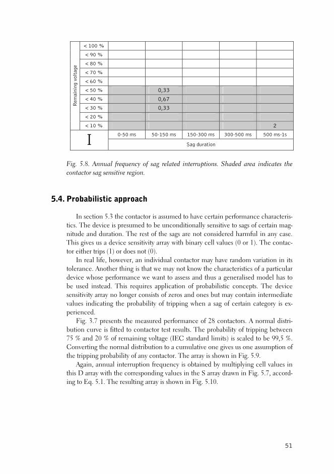
< 100 %
< 90 %
< 80 %
< 70 %
< 60 %
< 50 % 0,33
< 40 % 0,67
< 30 % 0,33
< 20 %
Rem
aini
ng v
olta
ge
< 10 % 2
0-50 ms 50-150 ms 150-300 ms 300-500 ms 500 ms-1s I Sag d ion urat
Fig. 5.8. Annual frequency of sag related interruptions. Shaded area indica s the contactor
5.4. Probabilistic approach
section 5.3 the contactor is assumed to have certain performance characteris-tics
lues (0 or 1). The contac-tor
actor may have random variation in its tolerance. Another thing is that we may not know the characteristics of a particular device whose performance we want to assessbe used instead. This requires application of probabilistic concepts. The device
ormance of 28 contactors. A normal distri-but f tripping between 75 % and 20 % of remaining voltage (IEC standard limits) is scaled to be 99,5 %. Converting the nthe tripping probability o
Again, annual interruption frequency is obtained by multiplying cell values in thi rd-ing to Eq. 5.1. The resulting array is shown in Fig. 5.10.
tesag sensitive region.
In. The device is presumed to be unconditionally sensitive to sags of certain mag-
nitude and duration. The rest of the sags are not considered harmful in any case. This gives us a device sensitivity array with binary cell va
either trips (1) or does not (0). In real life, however, an individual cont
and thus a generalised model has to
sensitivity array no longer consists of zeros and ones but may contain intermediate values indicating the probability of tripping when a sag of certain category is ex-perienced.
Fig. 3.7 presents the measured perfion curve is fitted to contactor test results. The probability o
ormal distribution to a cumulative one gives us one assumption of f any contactor. The array is shown in Fig. 5.9.
s D array with the corresponding values in the S array drawn in Fig. 5.7, acco
51

< 100 % 0,00 0,00 0,00 0,00 0,00
< 90 % 0,00 0,00 0,00 0,00 0,00
< 80 % 0,01 0,01 0,01 0,01 0,01
< 70 % 0,11 0,11 0,11 0,11 0,11
< 60 % 0,40 0,40 0,40 0,40 0,40
< 50 % 0,77 0,77 0,77 0,77 0,77
< 40 % 0,96 0,96 0,96 0,96 0,96
< 30 % 1,00 1,00 1,00 1,00 1,00
< 20 % 1,00 1,00 1,00 1,00 1,00
Rem
aini
ng v
olta
ge
< 10 % 1,00 1,00 1,00 1,00 1,00
0-50 ms 50-150 ms 150-300 ms 300-500 ms 500 ms-1s D Sag duration
Fig. 5.9. Contactor sag sensitivity. Probabilistic cell values.
< 100 %
< 90 %
< 80 % 0,02 0,03
< 70 % 0,33
< 60 % 0,40
< 50 % 0,25
< 40 % 0,64
< 30 % 0,33
Rem
aini
ng v
olta
ge
< 20 %
< 10 % 2,00
0-50 ms 50-150 ms 150-300 ms 300-500 ms 500 ms-1s I Sag duration
Fig. 5.10. Annual frequency of sag related interruptions.
The total annual number of interruptions is in this case: N = 4,01 (Eq. 5.2).
The binary sag sensitivity array in Fig. 5.8 gave a somewhat smaller value: N = 3,33. Probabilistic processing of data thus proved to have a strong effect on the re-sults. In general terms, the value of N depends on the location of non-zero cell values in S and D. Typically S has larger cell values on the upper rows whereas the sensitivity arrays usually have an emphasis on deep sags. Introducing probabilistic D arrays in such cases increases N in comparison to the binary approach.
s a matter of fact, the annual sag frequency array S iA s also a probabilistic quan-tity with measured and/or simulated numbers. S indicates how many sags there are to be expected in each category annually. The more measurement data we have or
52
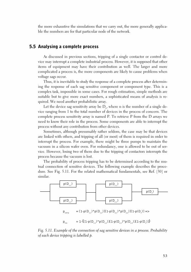
the m stive imulati at we ca t, the m enerally applica-ble the numbers are for that particular node of the network.
5.5 Analysing a complete process
s d in previous sect ripping ingle co r or co de-vi m upt a lete in l proces i posed that other items of equipment may have their contribution as well. The larger and more compl proc the mo ponents are likely to proble en voltag cur.
Thus, it is inevitable to study the respon lete process after determin-ing the response of each sag sensitive component or component type. This is a
ethods are means of analysis is re-
quired. We need another probabilistic array. e ice sag sensitivity array be Dn, where n is the number of a single de-
vice ranging from 1 to the total number of devices in the process of concern. The complete pro ess sensitivity array is named P. To retrieve P from the D arrays we need to know their role in the process. Some components are able to interrupt the pr ss t any c ribution her devi s.
ometimes, althou h presumably rather seld , the case ay be that vices are linked with others, and trippi r mo ) of them is required in o in ru xample, there might be three pumps to maintain the vacuum in a silicon wafer oven. For redundancy, one is allowed to be out of ser-vice. H , losing two of them due to the tripping of contactors interrupts the process because the vacuum is lost.
Th babilit ess s t i ng -tual co tion of sensitive devices. The f mple describes the proce-dur . See Fig. 5.11. For the related mathematical fundamentals, see Ref. [30] or
of each device tripping is labelled p.
ore exhau the s ons th rry ou ore g
Ace
discusse ions, t of a s ntacto ntrol ay interr comp dustria s. However, t is sup
icated a ess is, re com cause ms whe sags oc
se of a comp
complex task, impossible in some cases. For rough estimation, simple msuitable but to give more exact numbers, a sophisticated
L t the dev
c
oceS
ter
withou ont from ot ceg om m de
ng of all (o st rder topt the process. For e
owever
e pronnec
y of proc tripping ha o be determ ned accordi to the muollowing exa
esimilar.
p(D3)
p(D1,1
)
p(D1,2
)
p(D2,1
)
p(D2,2
)
pnotrip
= [1-p(D1,1
)*p(D1,2
)][1-p(D2,1
)*p(D2,2
)][1-p(D3)] =>
Fig. 5.11. Example of the connection of sag sensitive devices in a process. Probability
ptrip
= 1-{[1-p(D1,1
)*p(D1,2
)][1-p(D2,1
)*p(D2,2
)][1-p(D3)]}
53

Devices D1,1 and D1,2 are parallel, i.e. tripping of both of them interrupts the process. D2,1 and D2,2 make a similar pair whereas D3 is an independent branch. Thus tripping of either of the pairs or D3 brings the process down.
Calculating the probability of process tripping from the device sensitivity arrays rocess sensitivity array P. To any cell value
of P thus applies: D1,1, D1,1, D2,1, D2,2, and D3 gives us the p
( ) ( ) ( )[ ]j)(i,D1j)(i,Dj)(i,D1j)(i,Dj)(i,D11j)P(i, 32,22,11,21,1 −⋅⋅−⋅⋅−−= (5.3)
Generally written:
1...nj1...m,ij)(i,D11j)P(i,q
1k
r
1llk,
k
==∀⎥⎦
⎤⎢⎣
⎡⎥⎦
⎤⎢⎣
⎡−−= ∏ ∏
= =
mponents or component groups and rk is
f a sensitive component type ma
babilistic method described above to obtain mo
11, connected in series gives us a reduced form of Eq. 5.4:
(5.4)
where q is the number of serial connected co the number of parallel components in each group k in terms of Fig. 5.11. NOTE: The relationship between sensitive devices and their probabilistic con-
nections has to be determined individually for each study case. Otherwise the cal-culation results in an invalid process sensitivity array.
It is essential to note that increasing the number oy decrease the withstand level of the complete process significantly. This is es-
pecially important in systems where tripping of one component or a small sub-process is capable of bringing the whole plant down. The more these kind of com-ponents there are, the more possibilities there are to lose the process.
Instead of using some average or typical tolerance level for that particular equipment, we have to use the pro
re accurate figures. Let us take Fig. 5.9 presenting contactor sag sensitivity as an example. What happens if we have 10 or 100 of these in a process and tripping of any of them will cause a process shutdown? Assuming the contactors are, in terms of Fig. 5.
( ) ( ) ([ )]j)(i,D1j)(i,D1j)11j)P(i, n21(i,D −⋅⋅−⋅−−= ... (5.5)
In the case of n similar contactors (D1 = D = … = Dn) we can further simplify the expression:
2
( )[ ]n1 j)(i,D1− 1j)P(i, −= (5.6)
Let D1 be th system of e array shown in Fig. 5.9. Process sensitivity arrays for a 10, 100 and 1000 similar contactors are shown in Figs. 5.12-14, respectively.
54
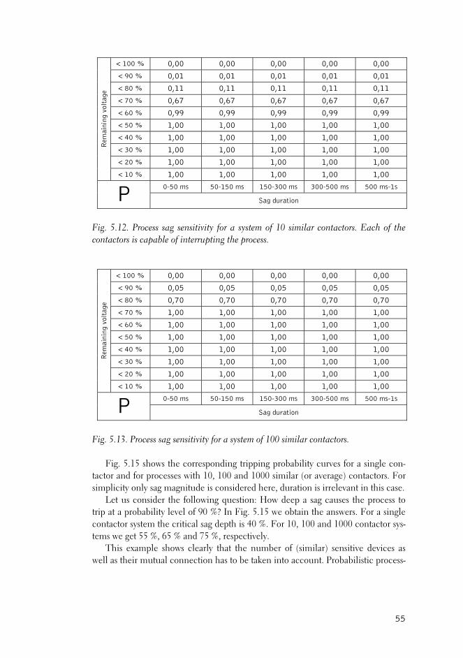
< 100 % 0,00 0,00 0,00 0,00 0,00
< 90 % 0,01 0,01 0,01 0,01 0,01
< 80 % 0,11 0,11 0,11 0,11 0,11
< 70 % 0,67 0,67 0,67 0,67 0,67
< 60 % 0,99 0,99 0,99 0,99 0,99
< 50 % 1,00 1,00 1,00 1,00 1,00
< 40 % 1,00 1,00 1,00 1,00 1,00
< 30 % 1,00 1,00 1,00 1,00 1,00
< 20 % 1,00 1,00 1,00 1,00 1,00
Rem
alt
age
inin
g vo
< 10 % 1,00 1,00 1,00 1,00 1,00
0-50 ms 50-150 ms 150-300 ms 300-500 ms 500 ms-1s P Sag duration
Fig. 5.12. Process sag sensitivity for a system of 10 similar contactors. Each of the contactors is capable of interrupting the process.
< 100 % 0,00 0,00 0,00 0,00 0,00
< 90 % 0,05 0,05 0,05 0,05 0,05
< 80 % 0,70 0,70 0,70 0,70 0,70
< 70 % 1,00 1,00 1,00 1,00 1,00
< 60 % 1,00 1,00 1,00 1,00 1,00
< 50 % 1,00 1,00 1,00 1,00 1,00
< 40 % 1,00 1,00 1,00 1,00 1,00
< 30 % 1,00 1,00 1,00 1,00 1,00
< 20 % 1,00 1,00 1,00 1,00 1,00
Rem
aini
ng v
olta
ge
< 10 % 1,00 1,00 1,00 1,00 1,00
0-50 ms 50-150 ms 150-300 ms 300-500 ms 500 ms-1s P Sag duration
Fig. 5.13. Process sag sensitivity for a system of 100 similar contactors.
Fig. 5.15 shows the corresponding tripping probability curves for a single con-
tacag magnitude is considered here, duration is irrelevant in this case.
Let us consider the following question: How deep a sag causes the process to trip at a probability level of contactor system the critical sag depth is 40 %. For 10, 100 and 1000 contactor sys-tem
ces as well as their mutual connection has to be taken into account. Probabilistic process-
tor and for processes with 10, 100 and 1000 similar (or average) contactors. For simplicity only s
90 %? In Fig. 5.15 we obtain the answers. For a single
s we get 55 %, 65 % and 75 %, respectively. This example shows clearly that the number of (similar) sensitive devi
55
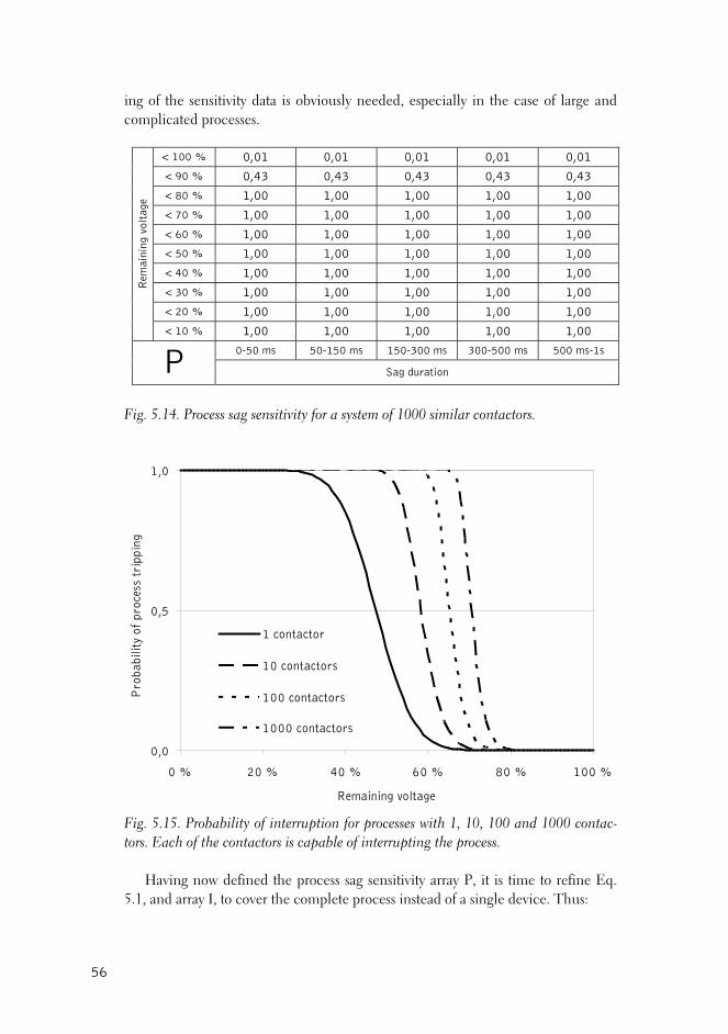
ing of itivit is obvi needed cially in ase of l nd compl roces
the sens y data ously , espe the c arge aicated p ses.
< 100 % 0,01 0,01 0,01 0,01 0,01
< 90 % 0,43 0,43 0,43 0,43 0,43
< 80 % 1,00 1,00 1,00 1,00 1,00
< 70 % 1,00 1,00 1,00 1,00 1,00
< 60 % 1,00 1,00 1,00 1,00 1,00
< 50 % 1,00 1,00 1,00 1,00 1,00
< 40 % 1,00 1,00 1,00 1,00 1,00
< 30 % 1,00 1,00 1,00 1,00 1,00
< 20 % 1,00 1,00 1,00 1,00 1,00
Rem
aini
ng
< 10 %
vol
tage
1,00 1,00 1,00 1,00 1,00
0-50 ms 50-150 ms 150-300 ms 300-500 ms 500 ms-1s P Sag duration
Fig. 5.14. Process sag sensitivity for a system of 1000 similar contactors.
ing the process.
5.1, and array I, to cover the complete process instead of a single device. Thus:
0,
obab
ility
of
proc
ess
trip
ping
5
1,0
1 contactor
10 contactors
Pr
100 contactors
1000 contactors
0,0
0 % 20 % 40 % 60 % 80 % 100 %
Remaining voltage
Fig. 5.15. Probability of interruption for processes with 1, 10, 100 and 1000 contac-tors. Each of the contactors is capable of interrupt
Having now defined the process sag sensitivity array P, it is time to refine Eq.
56
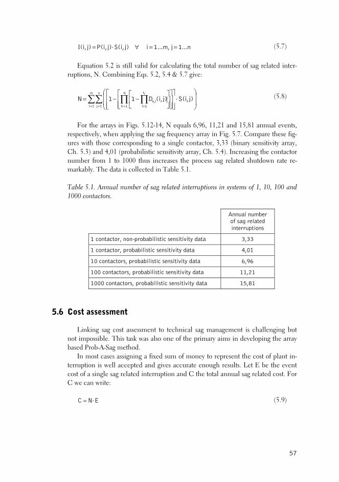
1...nj1...m,ij)S(i,j)P(i,j)I(i, ==∀⋅= (5.7)
Equation 5.2 is still valid for calculating the total number of sag related inter-ruptio mbi qs. 5.2, 5.7 giv
= ⎟⎟
⎠
⎞⋅
⎢ ⎢⎢⎣
⎡−=
r
1llk, j)S(i,(D1
k (5
o ays in . 5.12-1 quals 6, 1,21 an 1 annu ts, respectively, when applying the sag frequency n Fig. 5 mpare fig-ures with those corresponding to gle con , 3,33 (binary sensitivity array, Ch. 5. (probabilistic sensitivity array, Ch. 5.4). Increasing the tor numb 1 to us he do -marka e data is collected in Table 5.1
Ta e 5.1. Annual number of sag related interruptions in systems of 1, 10, 100 and
ns, N. Co ning E 5.4 & e:
∑∑⎜⎜⎢ ∏ ∏
= = ⎝ ⎣1i 1j = ⎣1k
⎛ ⎡m n
⎥⎦⎥⎦⎦⎥⎥⎥j)i,⎤⎤⎤
⎢ −1⎡q
N
F
.8)
r the arr Figs 4, N e 96, 1 d 15,8 al evenarray i .7. Co these
a sin tactor3) and 4,01 contacer frombly. Th
1000 th increases t process sag related shut wn rate re.
bl1000 contactors.
Annual number of sag related interruptions
1 contactor, non-probabilistic sensitivity data 3,33
1 contactor, probabilistic sensitivity data 4,01
10 contactors, probabilistic sensitivity data 6,96
100 contactors, probabilistic sensitivity data 11,21
1000 contactors, probabilistic sensitivity data 15,81
C we can write:
5.6 Cost assessment
Linking sag cost assessment to technical sag management is challenging but not impossible. This task was also one of the primary aims in developing the arraybased Prob-A-Sag method.
In most cases assigning a fixed sum of money to represent the cost of plant in-terruption is well accepted and gives accurate enough results. Let E be the eventcost of a single sag related interruption and C the total annual sag related cost. For
ENC ⋅= (5.9)
57
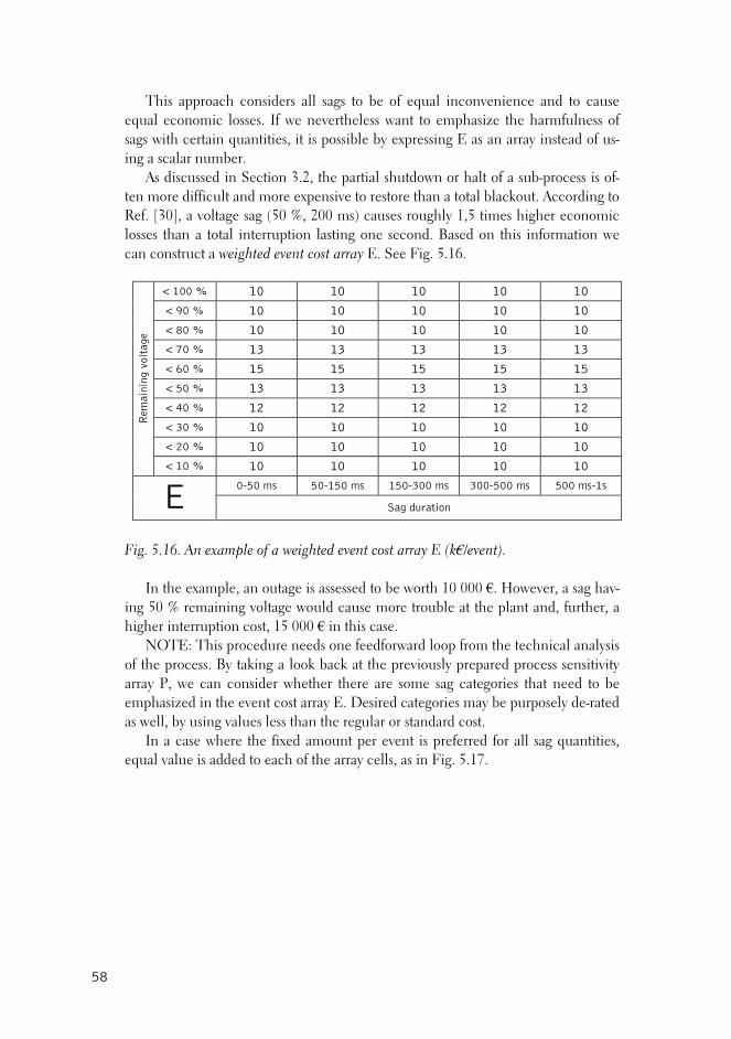
This approach considers all sags to be of equal inconvenience and to cause equal economic losses. If we nevertheless want to emphasize the harmfulness of sags with certain quantities, it is possible by expressing E as an array instead of us-ing a scalar number.
As discussed in Section 3.2, the partial shutdown or halt of a sub-process is of-ten
ghly 1,5 times higher economic losses than a total interruption lasting one second. Based on this information we can construct a weighted event cost array E. See Fig.
< 100 %
more difficult and more expensive to restore than a total blackout. According to Ref. [30], a voltage sag (50 %, 200 ms) causes rou
5.16.
10 10 10 10 10
< 90 % 10 10 10 10 10
< 80 % 10 10 10 10 10
< 70 % 13 13 13 13 13
< 60 % 15 15 15 15 15
< 50 % 13 13 13 13 13
< 40 % 12 12 12 12 12
< 30 % 10 10 10 10 10
< 20 % 10 10 10 10 10
Rem
aini
ng v
olta
ge
< 10 % 10 10 10 10 10
0-50 ms 50-150 ms 150-300 ms 300-500 ms 500 ms-1s E Sag duration
Fig. 5.16. An example of a weighted event cost array E (k€/e
In the exampl worth 10 000 €. However, a sag hav-
ing 50 % remaining vo trouble at the plant and, further, a higher i
NOT loop from the technical analysis of the p prepared process sensitivity array P, we can consider whether there are some sag categories that need to be emphasized in the event cost array E. Desired categories may be purposely de-rated
less than the regular or standard cost. fixed amount per event is preferred for all sag quantities,
equ
vent).
e, an outage is assessed to be ltage would cause more
nterruption cost, 15 000 € in this case. E: This procedure needs one feedforward
rocess. By taking a look back at the previously
as well, by using values In a case where theal value is added to each of the array cells, as in Fig. 5.17.
58
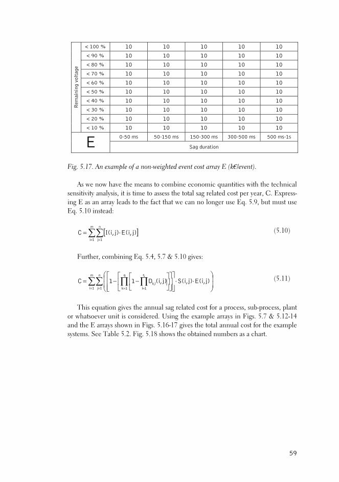
% 10 10 10 10 10 < 100
< 90 % 10 10 10 10 10
< 80 % 10 10 10 10 10
< 70 % 10 10 10 10 10
< 60 % 10 10 10 10 10
< 50 % 10 10 10 10 10
< 40 % 10 10 10 10 10
< 30 % 10 10 10 10 10
< 20 % 10 10 10 10 10
R
< 10 %
em
aini
ng v
olta
ge
10 10 10 10 10
0-50 ms 50-150 ms 150-300 ms 300-500 ms 500 ms-1s E Sag duration
Fig. 5.17. xample of a non-weighted event cost E (k€/event).
s w bine econ ic quantit ith the te ical sensitivity analysis, it is time to assess the total sag related cost year, C. ress-in ay lea the fact that we can n nger use Eq. 5.9, but must use E .1 d:
]
An e array A
g Eq. 5
e now have the means to com om ies w chn per Exp
as an arr ds to o lo0 instea
[∑∑ I(i,= =
Ej)C (5 0)
Fu ombining Eq. 5.4, 5.7 & 5.10
⎟⎜⋅⋅⎥⎢ ⎥⎢ ⎥⎢ −−= lk, j)E(i,j)S(i,j)(i,D11 .11)
ost for a process, sub-process, plant or
⋅=m n
1i 1j
rther, c
j)(i, .1
gives:
∑∑ ∏ ∏ ⎟⎞
⎜⎛ ⎤⎡ ⎤⎡ ⎤⎡m n q rk (5
= = = = ⎠⎝ ⎥⎦⎢⎣ ⎦⎣ ⎦⎣1i 1j 1k 1l
This equation gives the annual sag related c
C
whatsoever unit is considered. Using the example arrays in Figs. 5.7 & 5.12-14 and the E arrays shown in Figs. 5.16-17 gives the total annual cost for the example systems. See Table 5.2. Fig. 5.18 shows the obtained numbers as a chart.
59
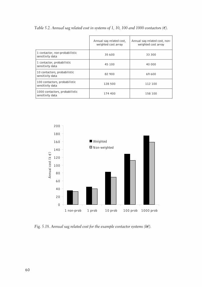
Table al sa ated cost i stems of 1 100 and 0 contacto ).
nual sag rela st, d cos ay
Annua related co on-ghted cost array
5.2. Annu g rel n sy , 10, 100 rs (€
Anweighte
ted cot arr
l sagwei
st, n
1 cosens
ntiti 35 60 33 300 actor, non-probabilistic
vity data 0
1 contacto bilistsensiti 45 10 40 000 r, proba ic
vity data 0
10 con robabilsensiti
82 90 69 600 tactors, p istic vity data
0
100 c s, probsensit a 128 500 ontactor
ivity databilistic 112 100
1000 contactors, probabilistic sensitivity data
174 400 158 100
Fig. 5.18. Annual sag related cost for the example contactor systems (k€).
0
80
100
120
160
180
1 non-prob 1 prob 10 prob 100 prob 1000 prob
Ann
ual c
ost
(k
200
Weighted
Non-weighted140
€)
20
40
60
60
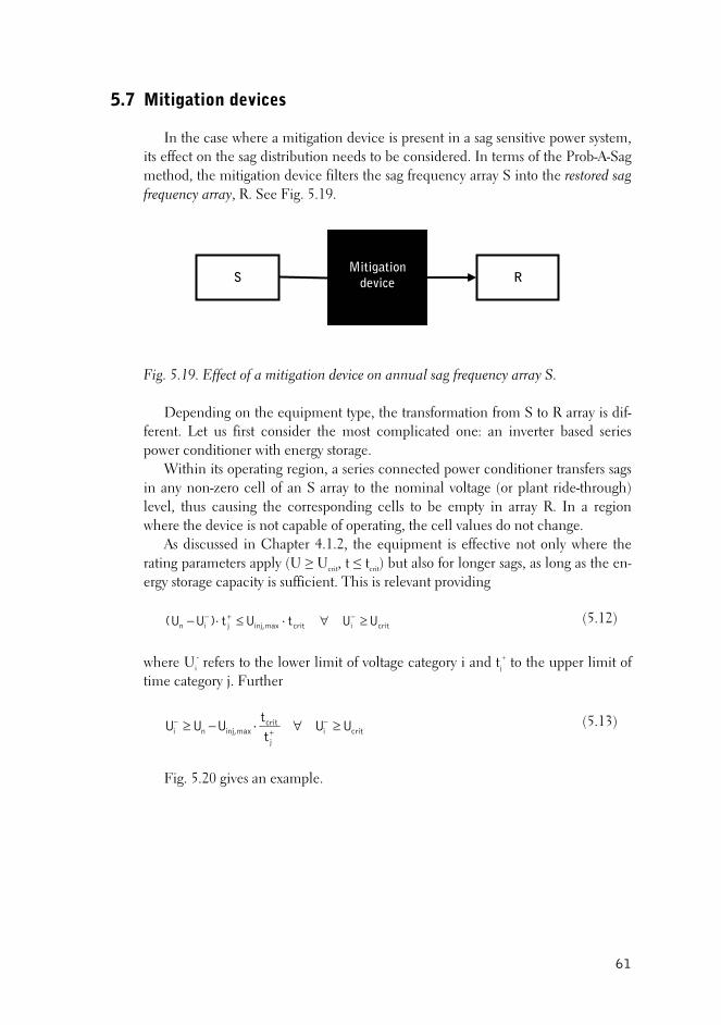
5.7
In the case where a mitigation device is pre its effect on the sag distribution nee method, the mitigation device filters the sag frequency array S into the restored sag f . 5.19.
Fig. 5.19. Effect of a mitigation device on annual sag frequency array S.
Depending on the equipment type, the transformation from S to R array is dif-series
pos
ugh)
(5.12)
where Ui- refers to the lower limit of voltage category i and tj
+ to the upper limit of time category j. Further
Mitigation devices
sent in a sagds to be considered. In
sensitive power system, terms of the Prob-A-Sag
requency array, R. See Fig
SMitigat
device ion
R
ferent. Let us first consider the most complicated one: an inverter based wer conditioner with energy storage. Within its operating region, a series connected power conditioner transfers sag
in any non-zero cell of an S array to the nominal voltage (or plant ride-throlevel, thus causing the corresponding cells to be empty in array R. In a region where the device is not capable of operating, the cell values do not change.
As discussed in Chapter 4.1.2, the equipment is effective not only where therating parameters apply (U ≥ Ucrit, t ≤ tcrit) but also for longer sags, as long as the en-ergy storage capacity is sufficient. This is relevant providing
criticritmaxinj,jin UUtUt)U(U ≥∀⋅≤⋅− −+−
critij
critmaxinj,ni UU
tt
UUU ≥∀⋅−≥ −+
− (5.13)
an example. Fig. 5.20 gives
61
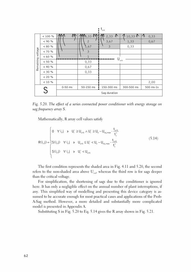
62
< 100 % 5,33 2,33 10,33 0,33
< 90 % 2 3,67 1,33 0,67
< 80 % 1,67 3 0,33
< 70 % 3
< 60 % 1
< 50 % 0,33
< 40 % 0,67
< 30 % 0,33
< 20 %
Rem
aini
ng v
< 10 % 2,00
olta
ge
0-50 ms 50-150 ms 150-300 ms 300-500 ms 500 ms-1s S Sag duration
tcrit
Ucrit
Fig. 5.20. The effect of a series connected power conditioner with energy storage on sag
atisfy
frequency array S. Mathematically, R array cell values s
⎪⎪⎪
⎩
⎨
<∋∀ −
+
criti
jmaxinj,nicrit
UUji,j)S(i,
tUUUUji,j)S(i,j)R(i,
⎪⎪⎪⎧
⋅−<≤∋∀
⋅−≥∧≥∋∀
= −
+−−
crit
j
critmaxinj,nicriti
t
tt
UUUUUji,0
(5.14)
The first condition represents the shadrefers to the non-shaded area above U , whereas the third row is for sags deeper
e shortening of sags due to the conditioner is ignored here. It has only a negligible effect on the annual number of plant interruptions, if any. This simplified way of modellsumed to be accurate enough for most practical cases and applications of the Prob-A-Sag method. However, a more detailed and substantially more complicated mo A.
Substituting S in Fig. 5.20 to Eq. 5.14 gives the R array shown in Fig. 5.21.
ed area in Fig. 4.11 and 5.20, the second
crit
than the critical voltage. For simplification, th
ing and presenting this device category is as-
del is presented in Appendix
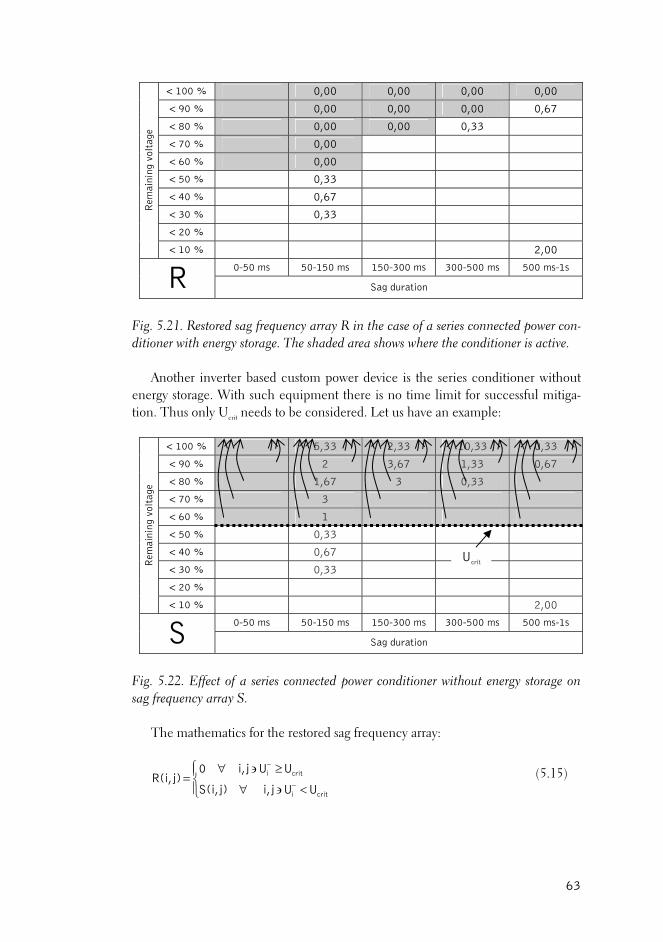
< 100 % 0,00 0,00 0,00 0,00
< 90 % 0,00 0,00 0,00 0,67
< 80 % 0,00 0,00 0,33
< 70 % 0,00
< 60 % 0,00
< 50 % 0 ,33
< 40 % 0 ,67
< 30 % 0,33
< 20 %
Rem
aini
ng v
olta
ge
2,00 < 10 %
0-50 ms 50-150 ms 150-300 ms 300-500 ms 500 ms-1s R Sag d ion urat
Fig. 5 stored sag frequency array R in series connected power con-ditioner with energy storage. The shaded area shows where the conditioner is active.
ased custom power device is the series conditioner without energy storage. With such equipment there is no time limit for successful mitiga-tion t us have an example:
< 100 %
.21. Re the case of a
Another inverter b
. Thus only Ucrit needs to be considered. Le
5,33 2,33 10,33 0,33
< 90 % 2 3,67 1,33 0,67
< 80 % 1,67 3 0,33
< 70 % 3
< 60 % 1
< 50 % 0,33
< 40 % 0,67
< 30 % 0,33
< 20 %
Rem
aini
ng v
olta
ge
< 10 % 2,00
0-50 ms 50-150 ms 150-300 ms 300-500 ms 500 ms-1s S Sag duration
Fig. 5.22. Effect of a series connected power conditioner without energy storage on sag frequency array S.
The mathematics for the restored sag frequency array:
⎪⎩
⎪⎨⎧
<∋∀
≥∋∀=
−
−
criti
criti
UUji,j)S(i,
UUji,0j)R(i, (5.15)
Ucrit
63
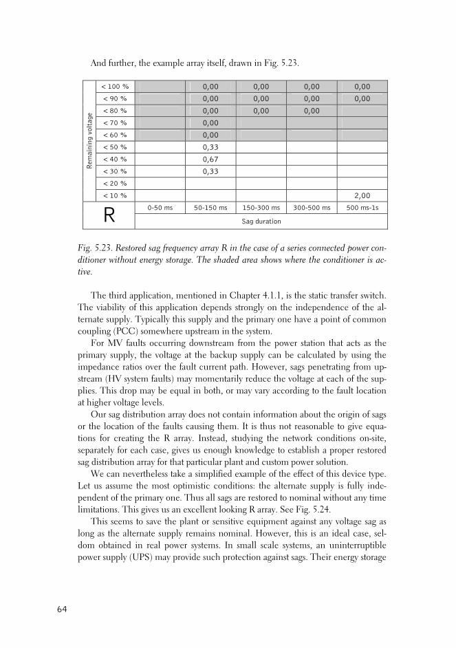
And further, the example arra , drawn . 5.23.
y itself in Fig
< 100 % 0,00 0,00 0,00 0,00
< 90 % 0,00 0,00 0,00 0,00
< 80 % 0,00 0,00 0,00
< 70 % 0,00
< 60 % 0,00
< 50 % 0,33
< 40 % 0, 67
< 30 % 0, 33
< 20 %
Rem
ain
2,00
ing
volt
age
< 10 %
0-50 ms 50-150 ms 150-300 ms 300-500 ms 500 ms-1s R Sag duration
Fig. 5.23. Restored sag frequency array R in the case of a series connected power con-diti
he third application, mentioned in Chapter 4.1.1, is the static transfer switch. The viability o ds strongly on the in dence al-ternate supply. Typically this supply and the primary one have a point of on co li ) somewhere upstream in the system.
o ccurring downstream from the power station that acts as the p ar , the voltage at the backup supply can be calculated by using the impedance ratios over the fault current path. H up-st stem faults) may momentarily reduce the voltage at each of the sup-pl . T p may be equal in both, or may vary accordin the fault lo n at higher voltage levels.
Our sag distributio array does t contain information ab t the orig or the on of the faults ca . ot to -tions for creating the R array. Instead, stu etwork conditions on-site, separately for each case, gives us enough knowledge to establish a proper restored
st optimistic conditions: the alternate supply is fully inde-pendent minal without any time lim Fig. 5.24.
This seems to save the plant or senslong as the alternate supply remainsdom obtained in real power systems. In small scale systems, an uninterruptible power supply (UPS) may provide such protection against sags. Their energy storage
oner without energy storage. The shaded area shows where the conditioner is ac-tive.
T
f this application depen depen of the comm
upF
rim
reamies
ng (PCCr MV faults oy supply
owever, sags penetrating from (HV syhis dro g to catio
n no ou in of sags locati using them It is thus n reasonable give equa
dying the n
sag distribution array for that particular plant and custom power solution. We can nevertheless take a simplified example of the effect of this device type.
Let us assume the moof the primary one. Thus all sags are restored to no
itations. This gives us an excellent looking R array. See itive equipment against any voltage sag as
nominal. However, this is an ideal case, sel-
64
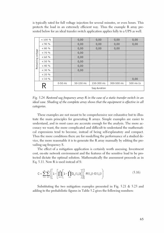
is t s, or even hours. This protects the load in an extremely efficient way. Thus the example R array pre-sented r an ideal transfer applic applies fully to a UPS as well.
ypically rated for full voltage injection for several minute
below fo switch ation
< 100 % 0,00 0,00 0,00 0,00
< 90 % 0,00 0,00 0,00 0,00
< 80 % 0,00 0,00 0,00
< 70 % 0,00
< 60 % 0,00
< 50 % 0,00
< 40 % 0,00
< 30 % 0,00
< 20 %
Rem
ain
ing
volt
age
< 10 % 0,00
0-50 ms 50-150 ms 150-300 ms 300-500 ms 500 ms-1s R Sag duration
Fig. 5.24. Restored sag frequency array R in the case of a static transfer switch in an ide ing of the complete array shows that the equipment is effective in all cat
mple examples are easier to un
al case. Shadegories. These examples are not meant to be comprehensive nor exhaustive but to illus-
trate the main principles for generating R arrays. Siderstand, and in most cases are accurate enough for the analysis. The more ac-
curacy we want, the more complicated and difficult to understand the mathemati-cal expressions tend to become, instead of being self-explanatory and compact. Thus the more conditions there are for modelling the performance of a studied de-vice, the more reasonable it is to generate the R array manually by editing the pre-vailing sag frequency S.
The effect of a mitigation application is certainly worth assessing. Investment cost, on-site network environment and the features of the sensitive load to be pro-tected dictate the optimal solution. Mathematically the assessment proceeds as in Eq. 5.11. Now R is used instead of S:
∑∑ ∏ ∏= = = = ⎟
⎟
⎠
⎞
⎜⎜
⎝
⎛⋅⋅
⎥⎥⎦
⎤
⎢⎢⎣
⎡⎥⎦
⎤⎢⎣
⎡⎥⎦
⎤⎢⎣
⎡−−=
m
1i
n
1j
q
1k
r
1llk, j)E(i,j)R(i,j)(i,D11C
k (5.16)
Substituting the two mitigation examples presented in Fig. 5.21 & 5.23 and adding to the probabilistic figures in Table 5.2 gives the following numbers:
65
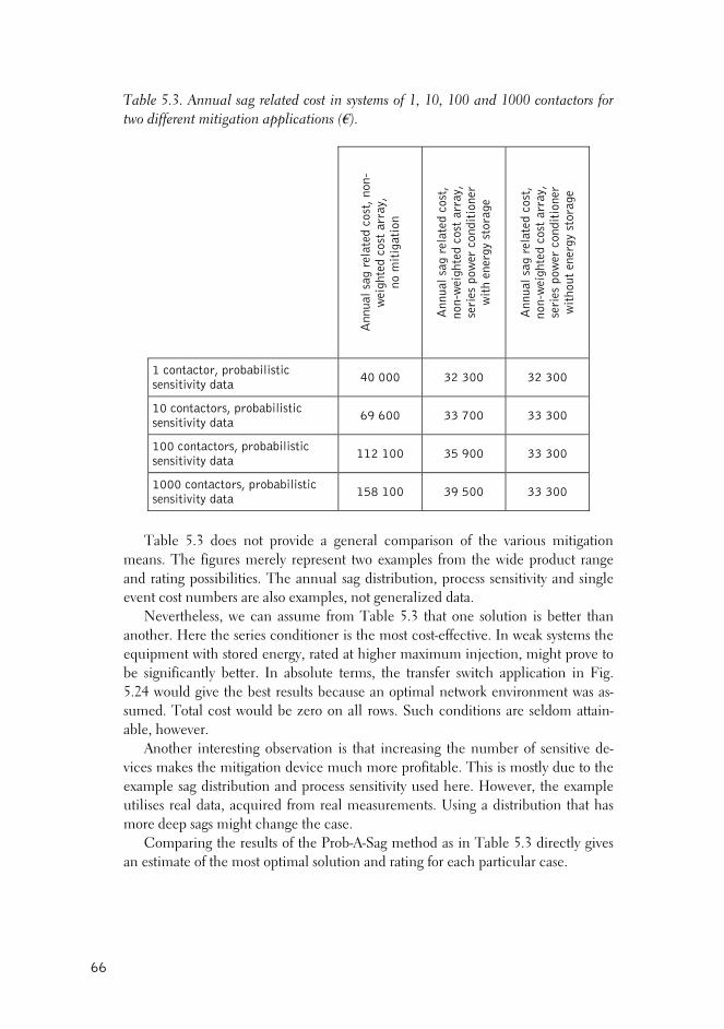
Table 5.3. Annual sag related cost in systems of 1, 10, 100 and 1000 contactors for two different mitigation applications (€).
Ann
ual s
ag r
elat
ed c
ost,
non
-w
eigh
ted
cost
arr
ay,
no m
itig
atio
n
Ann
ual s
ag r
elat
ed c
ost,
no
n-w
eigh
ted
cost
arr
ay,
seri
es p
ower
con
diti
oner
w
ith
ener
gy s
tora
ge
Ann
ual s
ag r
elat
ed c
ost,
no
n-w
eigh
ted
cost
arr
ay,
seri
es p
ower
con
diti
oner
w
itho
ut e
nerg
y st
orag
e
1 contactor, probabilistic sensitivity data
32 340 000 32 300 00
10 contactors, probabilistic 69 600 33 700 33 300 sensitivity data
100 contactors, probabilistic sensitivity data
112 100 35 900 33 300
1000 contactors, probabilistic 158 100 39 500 33 300 sensitivity data
Table 5.3 does not provide a general comparison of the various mitigation
means. The figures merely represent two examples from the wide product range and rating possibilities. The annual sag distribution, process sensitivity and single event cost numbers are also examples, not generalized data.
Nevertheless, we can assume from Table 5.3 that one solution is better than another. Here the series conditioner is the most cost-effective. In weak systems the equ
all rows. Such conditions are seldom attain-able, however.
Another interesting observation is that increasing the number of sensitive de-vices makes the mitigation device much more profitexample sag distribution and process sensitivity used here. However, the example utilises real data, acquired from real measurements. Using a distribution that has mo
gives an estimate of the most optimal solution and rating for each particular case.
ipment with stored energy, rated at higher maximum injection, might prove to be significantly better. In absolute terms, the transfer switch application in Fig. 5.24 would give the best results because an optimal network environment was as-sumed. Total cost would be zero on
able. This is mostly due to the
re deep sags might change the case. Comparing the results of the Prob-A-Sag method as in Table 5.3 directly
66
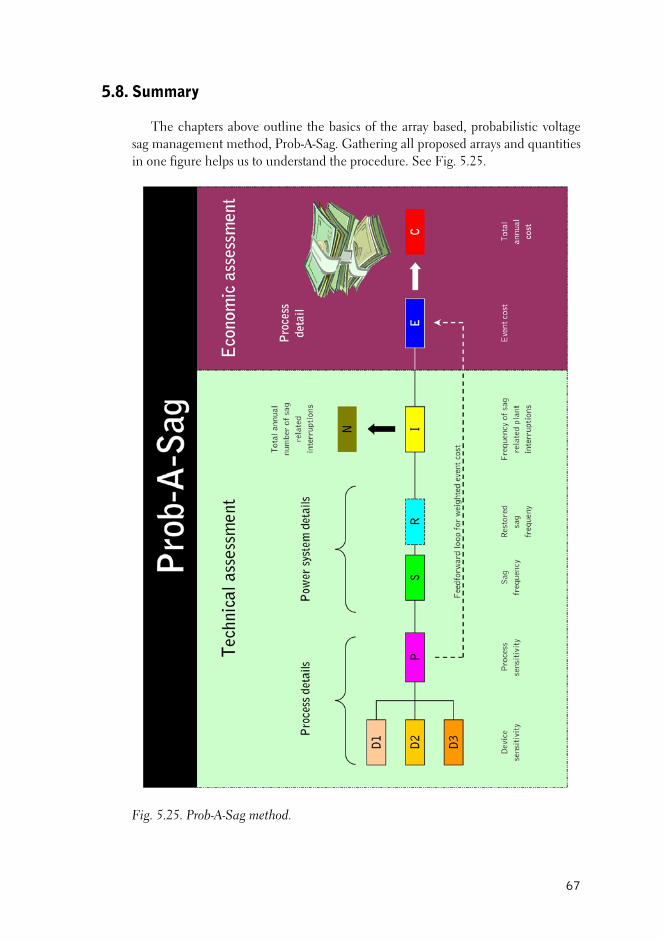
5.8.
he chapters above outline the basics of the array based, probabilistic voltage sag management method, Prob-A-Sag. Gathering all proposed arrays and quantities in one figure helps us to understand the cedure. See Fig. 5.25.
Fig. 5.25. Prob-A-Sag method.
Summary
T
pro
67
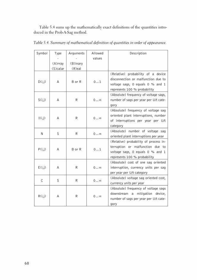
Table 5.4 sums up the mathematically exact definitions of the quantities intro-duced in the Prob-A-Sag method.
Symbol Type Arguments Allowed Description
Table 5.4. Summary of mathematical definition of quantities in order of appearance.
-
(A)rray
(S)calar
-
(B)inary
(R)eal
values
D(i,j) A B or R 0…1
(Relative) probability of a devi
disconnection or malfunction due to
voltage sags, 0 equals 0 % and 1
represents 100 % probability
ce
S(i,j) A R 0…∞
(Absolute) frequency of voltage sags,
number of sags per year per U/t cate-
gory
I(i,j) A R 0…∞
(Absolute) frequency of voltage sag
oriented plant interruptions, number
of interruptions per year per U/t
category
N S R 0…∞ (Absolute) number of voltage sag
oriented plant interruptions per year
P(i,j) A B or R 0…1
(Relative) probability of process in-
terruption or malfunction due to
voltage sags, 0 equals 0 % and 1
represents 100 % probability
E(i,j) A R 0…∞
(Absolute) cost of one sag oriented
interruption, currency units per sag
per year per U/t category
C S R 0…∞ (Absolute) voltage sag oriented cost,
currency units per year
R(i,j) A R 0…∞
(Absolute) frequency of voltage sags
downstream a mitigation device,
number of sags per year per U/t cate-
gory
68
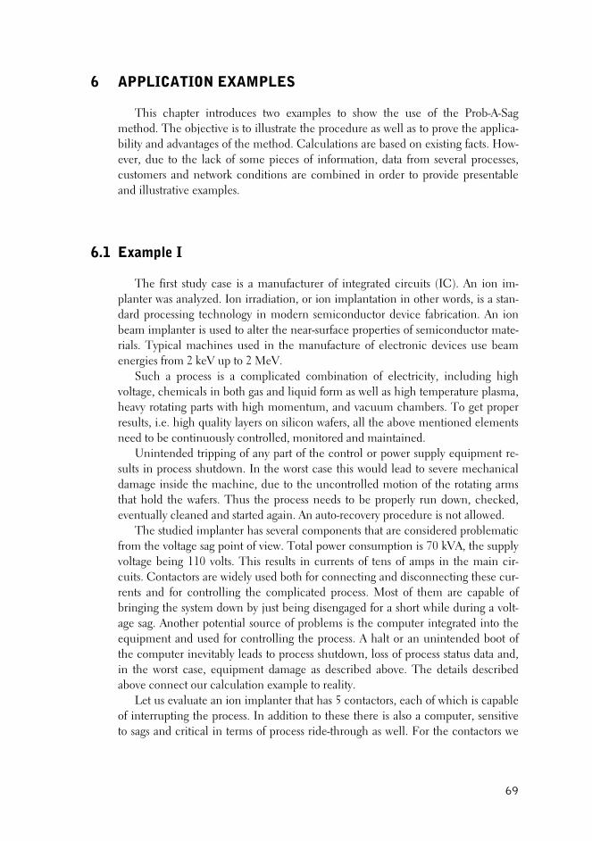
6 AP
his chapter introduces two examples to show the use of the Prob-A-Sag
bility and advantages of the method. Calculations are based on existing facts. How-e to ck iec rmation, data l processes, customers and network conditions a bined in order to provide presentable and illustra p
6.1 Example I
The first study case is a manufacturer of ipl as an zed. Ion adiation imdard processing technology in modern semiconductor device fabrication. An ion beam implanter is used to alter the near-surfacerials. Typical machines used in the ma factuenergies from eV up to
Such a process is a complicated combina lectricity, including high voltage, chemicals in both gas and liquid form heavy rotating parts with high mome and r results, i.e. high quality layers on silicon wafers need to be continuously controlled, monitored
ende rippin part consults in process shutdown. In the worst case th anical damage inside the machine, due to the unconthat hold the wafers. Thus the proc ds eventually cleaned and started again. An auto-re llowed.
The studied implanter has several componefrom e voltage sag poin view. T wer A, the supply voltage being 110 volts. This results in currencuits. Contactors are widely used both for connrents and for lling the complicated pro bringing the system down by just being disengaged for a short while during a volt-age sag. Another potential source of problems is the computer integrated into the equipment and used for controlling the process. A halt or an unintended boot of the computer inevitably leads to process shutdown, loss of process status data and, in the worst case, equipment damage as described above. The details described above connect our calculation example to reality.
Let us evaluate an ion implanter that has 5 contactors, each of which is capable of interrupting the process. In addition to these there is also a computer, sensitive to sags and critical in terms of process ride-through as well. For the contactors we
PLICATION EXAMPLES
Tmethod. The objective is to illustrate the procedure as well as to prove the applica-
ver, due the la of some p es of info from severare com
tive exam les.
ntegrated circuits (IC). An ion im-plantation in other words, is a stan-anter w aly irr , or ion
properties of semiconductor mate-re of electronic devices use beam
tion of e
nu2 k 2 MeV.
as well as high temperature plasma, vacuum chambers. To get propentum,
, all the above mentioned elementsand maintained. trol or power supply equipment re-is would lead to severe mech
Unint d t g of any of the
trolled motion of the rotating arms to be properly run down, checked, covery procedure is not a
ess nee
nts that are considered problematic consumption is 70 kV th t of otal pots of tens of amps in the main cir-ecting and disconnecting these cur-cess. Most of them are capable ofcontro
69

use probabilistic sensitivity, described in Fig. 5.9. The computer is assumed to be F-02, in terms of Fig. 3.11.
Let the contactor and PC sensitivity arrays be D1 and D2, respectively. D1 is shown in Fig. 5.9 and D2 is generated in Fig. 6.1.
< 100 % 0 0 0 0 0
< 90 % 0 0 0 0 0
< 80 % 0 0 0 0 0
< 70 % 0 1 1 1 1
< 60 % 0 1 1 1 1
< 50 % 0 1 1 1 1
< 40 % 0 1 1 1 1
< 30 % 0 1 1 1 1
< 20 % 0 1 1 1 1
Rem
aini
ng v
olta
ge
< 10 % 0 1 1 1 1
0-50 ms 50-150 ms 150-300 ms 300-500 ms 500 ms-1s D2 Sag duration
Fig. 6.1. Device sensitivity array for personal computer.
Applying Eq. 5.5 gives us the process sensitivity P:
[ ] [ ]{ }j)(i,D1j)(i,D11j)P(i, 25
1 −⋅−−= (6.1)
The corresponding P array is calculated in Fig. 6.2.
< 100 % 0,00 0,00 0,00 0,00 0,00
< 90 % 0,00 0,00 0,00 0,00 0,00
< 80 % 0,05 0,05 0,05 0,05 0,05
< 70 % 0,44 1,00 1,00 1,00 1,00
< 60 % 0,92 1,00 1,00 1,00 1,00
< 50 % 1,00 1,00 1,00 1,00 1,00
< 40 % 1,00 1,00 1,00 1,00 1,00
< 30 % 1,00 1,00 1,00 1,00 1,00
< 20 % 1,00 1,00 1,00 1,00 1,00
Rem
aini
ng v
olta
< 10 %
ge
1,00 1,00 1,00 1,00 1,00
0-50 ms 50-150 ms 150-300 ms 300-500 ms 500 ms-1s P Sag duration
Fig. 6.2. Process sensitivity array.
70
For the annual sag frequency we use the array in Fig. 5.7. Multiplying P and S cell by cell results in the interruption frequency array shown in Fig. 6.3.
< 100 % 0,00 0,00 0,00 0,00 0,00
< 90 % 0,00 0,00 0,00 0,00 0,00
< 80 % 0,00 0,08 0,15 0,02 0,00
< 70 % 0,00 3,00 0,00 0,00 0,00
< 60 % 0,00 1,00 0,00 0,00 0,00
< 50 % 0,00 0,33 0,00 0,00 0,00
< 40 % 0,00 0,67 0,00 0,00 0,00
< 30 % 0,00 0,33 0,00 0,00 0,00
< 20 % 0,00 0,00 0,00 0,00 0,00
Rem
aini
ng v
olta
ge
< 10 % 0,00 0,00 0,00 0,00 2,00
0-50 ms 50-150 ms 150-300 ms 300-500 ms 500 ms-1s I Sag d tion ura
Fig. 6 nual frequency of sag related inte
7,6. Supplying the process computer through a UPS would in this case reduce the number of interruptions to 5,8 ide-through capabilities, we could equip the contactors with intelligent control modules. They both distinguish sags from outages that require immedivoltage if a sag is detected. Only the control (coil) voltage is backed up and thus the all.
urther, the investment is also negligible compared to the case where we had to pro tal p demand e primary circuits (70 kVA). Rating the con-trol m or 50 kup gives us N = reasing alue to nd wo ld tely e ate the sag related interruptions. H r, allow ch a delay in equipment disconnect s to be carefully evaluated from th ec-ti o ew to damag
6.2 E m
This study case was founded on an Austrian master’s thesis analyzing the volt-age sa s of a ial c 36 s a o i re-calculate that particular process and its details but merely to utilize some of the rarely available data provided in the study. Key parameters, such as process sensitiv-
es were drawn from the tables in the ata for a study case since it was based on real
measurements recorded on-site. The total power requirement of the facility was
.3. An rruptions. Summation of the cell values in Fig. 6.3 gives N =
. If we would like to further improve the process r
ate tripping, and provide a sustained control
control module energy storage can be rated rather smF
tect the to ower of thodules f 0 ms bac 2. Inc the v 1 seco
u
on p
xa
comple limin oweve ing suion ha e prot
int of vi avoid es.
ple II
g issue n industr ustomer [ ]. There wa bsolutely n ntention to
ity, annual sag frequency and event cost figurthesis. This provides excellent d
71

me
he distribution of a total of 61 measured voltage sags is shown in Fig. 6.4. The magnitude and duration categories are selected according to the examples in Ch. 5. Num e con totals although the measureme iod w in mewh ger.
ntioned to be 20 MVA. However, no further details concerning the considered company or process were given, nor needed.
T
bers ar sidered to be annual nt peras,
fact, so at lon
< 100 % 4 1
< 90 % 9 1 2 2
< 80 % 9 6 11 1
< 70 % 1 2 1
< 60 % 1 2
< 50 % 1 1 2
< 40 % 1
< 30 %
< 20 % 1
Rem
aini
ng v
olta
ge
< 10 % 2
0-50 ms 50-150 ms 150-300 ms 300-500 ms 500 ms-1s S Sag duration
Fig. 6.4. Measured sag frequency.
When exposed to these 61 events, the process was interrupted 18 times. The
distribution of these critical events is shown in Fig. 6.5.
< 100 %
< 90 %
< 80 % 1 3 1
< 70 % 2 1
< 60 % 1 1
< 50 % 1 1 2
< 40 % 1
< 30 %
< 20 % 1
Rem
a
< 10 %
inin
g vo
ltag
e
2
0-50 ms 50-150 ms 150-300 ms 300-500 ms 500 ms-1s I Sag duration
Fig. 6.5. Recorded plant shutdowns due to voltage sags.
The probabilistic process sag sensitivity is now generated. Dividing the number
of shutdowns in each category by the total number of sags in that particular cate-
72

gory gives the probability of interruption and, further, the probabilistic process sen-sitivity.
0j)S(i,j)S(i,j)I(i,
j)P(i, ≠∀= (6.1)
The results of the calculation are presented in Fig. 6.6.
< 100 % 0,0 0,0
< 90 % 0,0 0,0 0,0 0,0
< 80 % 0,1 0,5 0,0 1,0
< 70 % 0,0 1,0 1,0
< 60 % 1,0 0,5
< 50 % 1,0 1,0 1,0
< 40 % 1,0
< 30 %
< 20 % 1,0
Re
mai
ning
vol
tage
< 10 % 1,0
0-50 ms 50-150 ms 300-500 ms 500 ms-1s 150-300 ms P Sag duration
Fig. 6.6. Probability of sag related interruptions as calculated according to Eq. 6.1.
eas of discontinuity. Based on experience regarding the typical shapes of sensitivity curves, and the explana-tions given in the original text source, the array was somewhat modified to provide contin d more alistic figur . The resulting P array is shown in Fig. .7.
Due to the relatively small sample there are some ar
uous an re es 6
< 100 % 0,0 0,0 0,0 0,0 0,0
< 90 % 0,0 0,0 0,0 0,0 0,0
0,0 0,5 0,5 0,1 < 80 % 1,0
< 70 % 0,0 0,1 1,0 1,0 1,0
< 60 % 0,0 1,0 1,0 1,0 1,0
< 50 % 0,0 1,0 1,0 1,0 1,0
< 40 % 0,0 1,0 1,0 1,0 1,0
< 30 % 0,0 1,0 1,0 1,0 1,0
< 20 % 0,0 1,0 1,0 1,0 1,0
Rem
aini
ng
< 10 %
vol
tage
0,0 1,0 1,0 1,0 1,0
0-50 ms 50-150 ms 150-300 ms 300-500 ms 500 ms-1s P Sag duration
Fig. 6.7. Probabilistic process sag sensitivity array.
73

Multiplying the arrays in Fig. 6.4 and 6.7 cell by cell gives the annual fre-quency of sag related interruptions to be expected. The resulting I array is shown in Fig. 6.8.
< 100 % 0,0 0,0 0,0 0,0 0,0
< 90 % 0,0 0,0 0,0 0,0 0,0
< 80 % 0,0 0,9 3,0 5,5 1,0
< 70 % 0,0 0,1 2,0 0,0 1,0
< 60 % 0,0 1,0 0,0 2,0 0,0
< 50 % 0,0 1,0 0,0 1,0 2,0
< 40 % 0,0 0,0 0,0 1,0 0,0
< 30 % 0,0 0,0 0,0 0,0 0,0
< 20 % 0,0 1,0 0,0 0,0 0,0
Rem
aini
ng v
olta
ge
< 10 % 0,0 2,0 0,0 0,0 0,0
0-50 ms 50-150 ms 150-300 ms 300 ms 500 ms-1s -500 I Sag d ion urat
Fig. 6. ency of g related interruptions.
Summing up all cell values of the arr .8 gives the total expected
number of shutdowns N = 24,5. Compared to the measured total of 18 interrup-f
0,0 or the P array cell [< 80 %, 300-500 ms] would have given N = 19. However, the
i-tude and duration. This means a non-weighted cost array can be used. In practice, multiplying the single event cost otal number of interruptions, N, gives the annua hus t tal cost case whe o mitiga is used would be 6 125 r year
s ries c cted power conditioner would provide some help. The benefit gained depends on the device rating, with the maximum injec and am n ed en being the main parameters. Accor to the reference, the tot r requ by the c er shoul protecte ainst sags as well, i. e oner ld be rated at 20 MVA. Typically, o small fr of the tot s sens to sags an a lower r is allow r the con ner. Assuming that the w plant ac y needs t protected, we can estimate the effect power conditioner rating. Annual sag cost figures are show 6.1.
8. Frequ sa
ay in Fig. 6
tions, this estimate is high but still realistic. Using the calculated sensitivity value o fre has to be some inaccuracy or error in the original data because such a sensi-
tivity curve shape is not considered likely. In the thesis, a hypothetical but presumably relevant event cost value has been
used, i.e. 250 000 €. The cost was assumed to be equal, regardless of the sag magn
by the tl cost. T he to in a re n tion 000 € pe .
U
ou
e. th
ing a se onnetion
t of stor ergy ding al powe ired ustom d be d ag conditi shou nly a actional load i itive d so ating ed fo ditio
hole tuall o be of the n in Table
74

Table 6.1. Annual sag cost obtained by using different mitigation device ratings (k€). Without mitigation the cost would be 6 125 k€.
Injection 150 ms 300 ms 500 ms Infinite
30 % 5 900 5 150 3 775 3 525 50 % 5 625 4 375 2 50 2 000 0 80 % 5 375 4 125 1 750 750
100 % 5 125 3 375 1 000 0
A
uch
Ln fo
s learly in Tabl , in this case increasing the injection time is m ffectiv n increa the magnitude. Naturally, this depends on the original sag distribution and is assumed ply gene
e the example a step further. A mitigation device rated at 50 jec-tio s wou nd feasible solut Such equipment would the an l cost from 25 to 2 500 k€, i.e. wo save 3 62sumin dgeta ice to be €/kVA, MVA unit would thu st 4 M€. In r word yba ul an an . In practice, some expenses have to be calculated for eventual substation and switchgear re-arrangement, maintenance, losses, etc. Nevertheless, a power condi-
e knew more about the process and ty of a transfer
swi
can be c seen e 6.1more e e tha sing
not to ap rally.t us take % inr 500 m ld be both a realistic a ion. reduce nua 6 1 uld 5 k€. As-g the bu ry pr 200 a 20 s co othe s, the pa ck time wo d be less th 2 years in ideal case
tioner appears to be a well justified option. If wthe power system supplying it, we could also estimate the feasibili
tch by using the Prob-A-Sag method.
75
7
aving outlined and applied the Prob-A-Sag method to two test cases, it is time for eva riticis iscussio espect t develop eds.
The primary aim of the task was to de a method ould com nd assess the effects, cost as nd mitig f voltage sags in a successful and flexible way. These object re listed pter 5.2:
of highly unsymmetrical faults and 3-phase loads, a more sophisticated approach has to be developed for cases where ac-curate results are required.
One solution would be to utilize the 3-phase sag characterization method men-tioned in Chapter 2.4. instead of using single phase sag magnitude and duration as the sag parameters. In such arrays there should be separate dimensions for sag type (including subtype), characteristic voltage phasor (amplitude and angle) as well as the positive-negative factor, which is also a phasor. This leads to a complicated yet presumably accurate and widely applicable calculation. However, it could by no means be considered illustrative or a simple-to-use method for the utility person-nel. This is why the 3-phase approach was not used here, but is certainly worth considering in the future development of the method.
This is relevant especially in the case of adjustable speed drives. However, their sag sensitivity can roughly be expressed by using single-phase quantities or the av-erage value of the rms phase-to-ground voltages during a sag. In addition, a supply-ing LV feeder is typically protected by a contactor that has to be analysed as a sin-gle-phase component. Beyond this exception, the method using single-phase sag distribution data is applicable to any size and type of power system.
Selecting the array resolution gives flexibility, although very small or large reso-lutions do not seem to be reasonable according to our experience. Too small arrays are not accurate enough. At the other extreme, the currently available initial data (sag distribution, device sensitivity, etc.) does not support very large scale arrays.
DISCUSSION
Hluation, c m and d n with r o future ment ne
velop that c bine apects a ation oives we in Cha
- all quantities should be presented in a uniform format - applicable to all environments from a single customer to a complete power
distribution system - flexible accuracy from a rough estimate to exact numbers - must allow for probabilistic processing of data - possibility to be implemented in power system software platforms - includes tools for investigating custom power applications and other means
of mitigation The format was chosen to be an array. All quantities were presented in this
format. Sags were considered from the point of view of a single-phase device. This approach is also applicable to 3-phase equipment as long as the sags are substan-tially symmetrical. For the combination
76

The fact that voltage sags are seldom rectangular in shape has also to be noted when assessing the method accuracy.
we
n. Another task is to add mo quantities to describe voltage sag properties (distortion, unbalance, phase an-gle jum e array dimension from 2 mension a
Usin approach to be applied nown, integer value arrays may be he prob-abilisticmethod d er the option of a partial process shutdown; only a binary trip/non-trip approach is applied. Dividing the complete process into sub-processes wh
sophisticated analysis application. In this thesis the spr
he effect of practically any pow
enough for as-ses
Two features related to the method flexibility and accuracy were purposely left for future research and development. In sag sensitivity tests, the equipment samples
re quite small. Generating comprehensive libraries for all sensitive devices and device types involves too much work for a single research group or university. Fu-ture co-operation is needed for providing this informatio
rep, etc.) This would be made possible by increasing thto a higher number. Each new quantity would require adding a new di-
s well. g non-integer cell values in arrays enables a probabilistic
. If some of the quantities are not sufficiently k used together with the probabilistic ones. In complex processes t connection between all sensitive devices is quite a task to carry out. This
oes not consid
ich only have two stages (on/off) is one solution that enables more accurate analysis. Introducing a weighted event cost array gives another viable approach to this issue. In the future this feature could be further developed within the Prob-A-Sag method as well.
In practice, the analysis can be done with pen and paper, with spreadsheet software or with any more
eadsheet has been used. Nevertheless, no quantities or operations that are not available or can not be implemented in modern power system analysis software were needed nor used. Some features, such as the annual sag distribution, could be directly computed by using the network component database. Due to the selected scope of the study this application was not tested. However, similar calculations have been successfully implemented and tested for other purposes. One could therefore assume they are also applicable to the Prob-A-Sag method.
Some examples of custom power equipment were given in Chapter 5 and of these, some were also included in the case studies. T
er conditioner can be easily taken into account in the Prob-A-Sag method. The more accurate the results required, the more complicated the arrays and, espe-cially, their mathematical expressions will become. It was not reasonable to in-clude extremely detailed models of all available solutions and their variations and ratings. Nevertheless, the basic principles required for generating R arrays for dif-ferent device types were provided. These are assumed to be accurate
sing the type, rating and cost/benefit figures of such a vast investment.
77

8
a “common language”, the arrays, but also enables probabilistic pro
mportant for future case studies. In cases where it is not possi-ble
CONCLUSION
This doctoral thesis considers voltage sags, their technical and economic im-pact as well as their mitigation. All these topics have been earlier introduced to academic society, along with various methods to analyse, assess and optimise the phenomena related to them.
However, the means to combine all of them in a mathematically exact yet prac-tically applicable way has not been proposed. The research efforts on which this publication has been based eventually culminate in the outline of the array based Prob-A-Sag method. It is a tool that not only expresses all quantities mentioned above in terms of
cessing of the data. Freely scalable arrays enable freely adjustable resolution as well. Due to the exact and yet simple mathematical expression of the quantities, the Prob-A-Sag method can be easily implemented in practically any platform, from spreadsheet applications to the most up-to-date network management soft-ware. This method is considered to be the main contribution of the thesis.
In addition to the Prob-A-Sag method there are two more aspects worth men-tioning in terms of their contribution to power systems engineering and voltage sag research. The work included tests for several device categories, aiming to study their sensitivity to voltage sags. This kind of information, i.e. device sensitivity li-braries, is extremely i
to measure the sag response of a particular device or process, these general li-braries may be used for estimating the sensitivity. The more data we have, the more comprehensive and relevant analysis results we can achieve.
As a third piece of novel scientific information, this publication provides dis-cussion and calculations on the feasibility and network requirements of modern sag mitigation equipment, i.e. custom power technology.
78
REFERENCES
EN 50160. Voltage characteristics of electricity supplied by public distribution systems. Cenelec, Brussels, Belgium, November 1999.
IEEE Std. 1159-1995. IE
[1]
[2]
[3]
[4]
[5]
[6]
[7] f AC contactor
[8] wer system disturbances on AC-coil contactors. IEEE 1997 Annual Textile, Fiber, and Film Industry Technical Conference, 1997. 6 p.
[9] Koch, R. G., Petroianu, A. A design methodology for optimising utility power system and industrial plant voltage dip / supply interruption compatibility. Afri-con ’96, Stellenbosch, South Africa, 24-27 September 1996, pp. 260-265.
[10] Gosbell, V. J., Smith, V., Robinson, D. A., Perera, B. S. P., Coulter, R. Sag test-ing of dairy farm milking equipment. PowerCon 2000, International Confer-ence on Power System Technology, 2000, Volume 2, pp. 947-952.
[11] McGranaghan M. F., Mueller D. R., Samotyj M. J. Voltage sags in industrial systems. IEEE Transactions on Industry Applications, Volume 29, Issue 2, March-April 1993, pp. 397-403.
[12] IEEE Std. 1346-1998. IEEE recommended practice for evaluating electric power system compatibility with electronic process equipment. IEEE, July 1998. vi + 37 p.
EE recommended practice for monitoring electricpower quality. IEEE, November 1995. vi + 70 p.
Heine, P., Lehtonen, M. Voltage Sags Caused by Faults at Different Power Sys-tem Levels and Experienced by Low Voltage Customers. PMAPS 2002, The 7th International Conference of Probabilistic Methods Applied to Power Systems, Naples, Italy, September 22-26, 2002, pp. 563-568.
Zhang, L. D., Bollen, M. H. J. Characteristic of Voltage Dips (Sags) in Power Systems. IEEE Transactions on Power Delivery, Volume 15, Issue 2, April 2000, pp. 827-832.
Bollen, M. H. J., Styvaktakis, E. Characterization of Three-Phase Unbalanced Dips (as easy as one-two-three?). IEEE Power Engineering Society Summer Meeting, Volume 2, Seattle, WA, USA, 16-20 July, 2000, pp. 899-904.
IEC 60947-4-1. Low-voltage switchgear and controlgear - Part 4-1: Contactors and motor-starters - Electromechanical contactors and motor-starters. IEC. Ge-neva, Switzerland, 2000. 177 p.
Collins, E. R. Jr., Zapardiel, F. An experimental assessment obehavior during voltage sags. ISIE '97, Proceedings of the IEEE International Symposium on Industrial Electronics, Volume 2, 1997, pp. 439-444.
Collins, E. R. Jr., Bridgwood, M. A. The impact of po
79

[13] IEC 61167. Metal halide lamps. IEC, Geneva, Switzerland, September 1992. 51 p.
[17] , Switzerland, January 2000.
[18] cent lamps) - Performance requirements. IEC, Geneva,
[19] s., IEEE
[20] oltage dips and sensitivity of consumers in low
[21] C, USA,
[22] art 1: Rating specifications, particularly for
[23] power
[24] quency a.c.
[25] ific test methods. IEC, Geneva, Switzerland,
[14] C 60188. High-pressure mercury vapour lamps - Performance specifications. IEC, Geneva, Switzerland, May 2001. 74 p. IE
[15] IEC 60192. Low-pressure sodium vapour lamps - Performance specifications. IEC, Geneva, Switzerland, May 2001. 54 p.
[16] IEC 60662. High-pressure sodium vapour lamps. IEC, Geneva, Switzerland,January 1980. 252 p.
IEC 60927, ed. 2.1. Auxiliaries for lamps - Starting devices (other than glow starters) - Performance requirements. IEC, Geneva59 p.
IEC 60923, ed. 2.1. Auxiliaries for lamps - Ballasts for discharge lamps (exclud-ing tubular fluoresSwitzerland, November 2001. 51 p.
Dorr D. S., Mansoor A., Morinec A. G., Worley J. C. Effects of power line volt-age variations on different types of 400-W high-pressure sodium ballastTransactions on Industry Applications, Volume 33 Issue 2, March-April 1997. pp. 472-476.
Brauner G., Hennerbichler C. Vvoltage networks. CIRED 2001, 18-22 June 2001, Amsterdam, The Nether-lands. IEE Conference Publication No. 482, 2.31, 5 p.
ITI curve. Information Technology Industry Council, Washington D2000. (http://www.itic.org/technical/iticurv.pdf)
IEC 61136-1. Semiconductor power convertors - Adjustable speed electric drive systems - General requirements - Pd.c. motor drives. IEC, Geneva, Switzerland, April 1992. 67 p.
IEC 61800-1. Adjustable speed electrical power drive systems - Part 1: General requirments - Rating specifications for low voltage adjustables speed d.c. drive systems. IEC, Geneva, Switzerland, December 1997. 201 p.
IEC 61800-2. Adjustable speed electrical power drive systems - Part 2: General requirements - Rating specifications for low voltage adjustable frepower drive systems. IEC, Geneva, Switzerland, March 1998. 175 p.
IEC 61800-3. Adjustable speed electrical power drive systems - Part 3: EMC product standard including specJune 1996. 171 p.
80

[26] IEC 60146-1-1. Semiconductor convertors - General requirements and line commutated convertors - Part 1-1: Specifications of basic requirements. IEC,
[27] nd line
f Power, Rio de Janeiro, Brazil, October 6-9, 2002.
[29] Stockman, n motor drive under voltage sag conditions. ICHQP 2002, 10th
[30] för elavbrott. TemaNord 1994:627,
[31] IEEE Transactions on Power Systems,
[32]
[36] Abhilfemass-
Geneva, Switzerland, April 1991. 135 p.
IEC 60146-1-2. Semiconductor convertors - General requirements acommutated convertors - Part 1-2: Application guide. IEC, Geneva, Switzer-land, April 1991. 187 p.
[28] Cao, R., Collins E. R. Jr. The Effects of Load Types on the Behavior of AC Mo-tor Drives During Voltage Sags. ICHQP 2002, 10th International Conference on Harmonics and Quality o6 p.
K., D’hulster, F., Desmet, J., Belmans, R. J. M. Torque behaviour of a RFO inductioInternational Conference on Harmonics and Quality of Power, Rio de Janeiro, Brazil, October 6-9, 2002. 6 p.
Lemström B., Lehtonen M. KostnaderNordisk Ministerråd, Copenhagen, 1994. 165p. (in Swedish, summary also in English).
Heine, P., Pohjanheimo, P., Lehtonen, M., Lakervi, E. A method for estimating the frequency and cost of voltage sags.Volume 17, Issue 2, May 2002. pp. 290-296.
Hingorani, N.G. Introducing custom power, IEEE Spectrum, Volume 32, Issue 6, June 1995. pp. 41-48.
[33] Technical Brochure: Custom Power – State of the art. Cigre Working Group 14.31, Paris, France, August 2002. 110 p.
[34] Kreyszig, E. Advanced Engineering Mathematics, 8th ed. John Wiley & Sons, Inc, USA, 1999. 1156 p.
[35] IEEE P1346 Working Group homepage. http://grouper.ieee.org/groups/1346/ points.html. Updated: October 11, 2001.
Haber, A. Analyse von Spannungseinbrüchen und mögliche nahmen in einem Industriebetrieb. Master’s thesis. Graz University of Tech-nology, Graz, Austria, June 2001. 103 p.
81
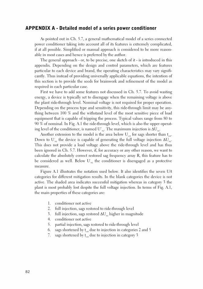
APPENDIX A - Detailed model of a series power conditioner
As pointed out in Ch. 5.7, a general mathematical model of a series connected poif aab
or, to be precise, one sketch of it - is introduced in this appacathis section is to provide the seeds for brainwork and refinement of the model as
entheDepending sensitivity, this ride-through limit may be any-hi
eq90 nal. In Fig. A.1 the ride-through level, which is also the upper operat-ing
Do g the full voltage injection ∆Uinj. This does not provide a load voltage above the ride-through level and has thus beca ect restored sag frequency array R, this feature has to beme
Figure A.1 illustrates the notation used below. It also identifies the seven U/t caactive. The shaded area indicates successful mitigation whereas in category 3 the plathe
inj higher in magnitude 4. conditioner not active 5. partial injection, sags restored to ride-through level 6. sags shortened by tcrit due to injection in categories 2 and 5 7. sags shortened by tcrit due to injection in category 3
wer conditioner taking into account all of its features is extremely complicated, t all possible. Simplified or manual approach is considered to be more reason-
le in most cases and hence is preferred by the author. The general approach -
pendix. Depending on the design and control parameters, which are features rticular to each device and brand, the operating characteristics may vary signifi-ntly. Thus instead of providing universally applicable equations, the intention of
required in each particular case. First we have to add some features not discussed in Ch. 5.7. To avoid wasting
ergy, a device is typically set to disengage when the remaining voltage is above plant ride-through level. Nominal voltage is not required for proper operation.
on the process type and t ng between 100 % and the withstand level of the most sensitive piece of load
uipment that is capable of tripping the process. Typical values range from 80 to % of nomi level of the conditioner, is named U+
inj. The maximum injection is ∆Uinj. Another extension to the model is the area below Ucrit for sags shorter than tcrit. wn to U-
inj the device is capable of generatin
en ignored in Ch. 5.7. However, if, for accuracy or any other reason, we want to lculate the absolutely corr considered as well. Below U-
inj the conditioner is disengaged as a protective asure.
tegories for different mitigation results. In the blank categories the device is not
nt is most probably lost despite the full voltage injection. In terms of Fig. A.1, main properties of these categories are:
1. conditioner not active 2. full injection, sags restored to ride-through level 3. full injection, sags restored ∆U
82
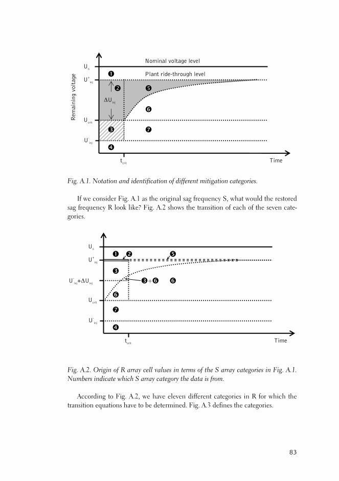
Fig. A.1. Notation and identification of different mitigation categories. If we consider Fig. A.1 as the original sag frequency S, what would the restored
sag frequency R look like? Fig. A.2 shows the transition of each of the seven cate-gories.
Fig. A.2 r n Fig. A.1. Number
cco in
transition equations have to be determined. Fig. A.3 defines the categories.
. O igin of R array cell values in terms of the S array categories i s indicate which S array category the data is from.
A rd g to Fig. A.2, we have eleven different categories in R for which the
Rem
aini
ng v
olta
ge
Time
Plant ride-through level
tcrit
Ucrit
U+
inj
Un
Nominal voltage level
∆Uinj
U-
inj
Time tcrit
Ucrit
U+
inj
Un
+
U-
inj
U-
inj+∆U
inj
83
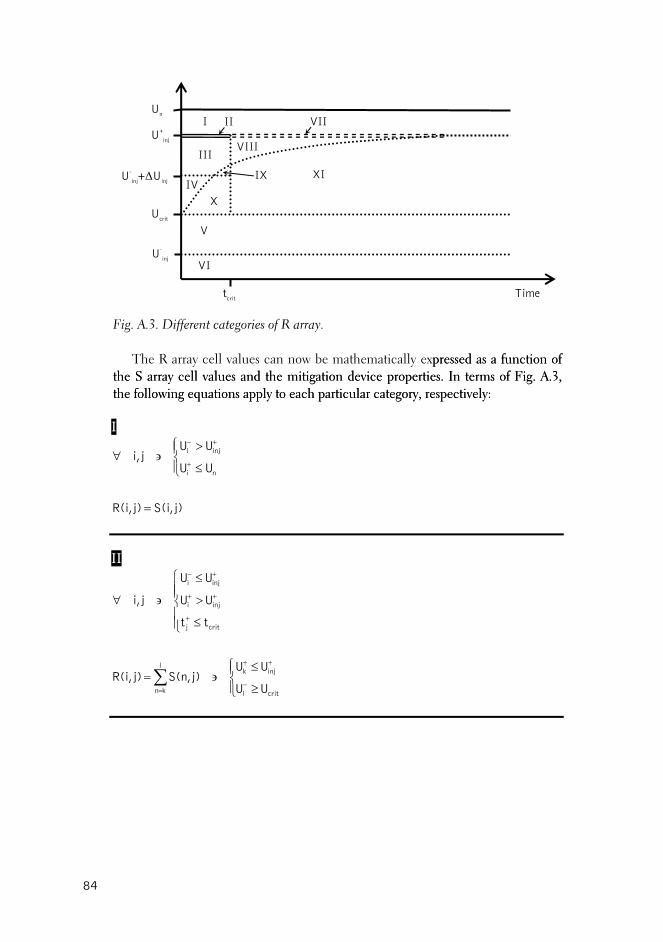
Fig. A.3. Different categories of R array.
a function of the S array cell values and the mitigation device properties. In terms of Fig. A.3, the
a function of the S array cell values and the mitigation device properties. In terms of Fig. A.3, the
The R array cell values can now be mathematically expressed as pressed as
following equations apply to each particular category, respectively: following equations apply to each particular category, respectively:
I
j)S(i,j)R(i,
UU
UUji,
ni
inji
=
⎪⎩
⎪⎨⎧
≤
>∋∀
+
+−
II
⎪⎩ ≥
≤∋=
⎪⎪⎩
⎪⎪⎨
⎧
≤
∋∀
−
++
=
+
+
−
∑critl
injkl
kn
critj
i
i
UU
UUj)S(n,j)R(i,
tt
U
U
ji,
⎪⎨⎧
> +injU
≤ +injU
Time tcrit
Ucrit
+
injU
Un
U-
inj
I II
V
X
I
VII
III
VI
X XI U-
inj+∆U
inj
VIII
IV
84
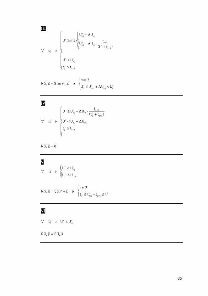
III
⎩⎨⎧
<+≤
∈∋+=
⎪⎪⎪⎪
⎩
⎪⎪⎪⎪
⎨
⎧
≤
85
<+
⎪⎩
⎪⎨x
⎧
+⋅
+≥
∋∀
+−+
−
+
+
++
−
−
iinjimi
critj
i
critj
critinj
injinj
i
UUUU
Zmi,S(mj)R(i,
tt
UU
)t(t
tUU
UU
aU
ji,
∆
∆
∆
m−inj
inj
j)
IV
0j)R(i,
tt
t
critj
=
⎪⎪⎩
⎧
≤
UUU
)t(tUUU
ji, injinji
critj
critinjinji
⎪
⎪⎪⎪
⎨ +<
+⋅−≥
∋∀+
−+
++−
∆
∆
V
+++
−
+
−−
jcritjnj
criti
inji
tttt
Znj)nS(i,j)R(i,
UU
UUji,
⎩⎨⎧
≤−≤
∈∋+=
⎪⎩
⎪⎨⎧
<
≥∋∀
VI
−+
j)S(i,j)R(i,
UUji, inji
=
<∋∀
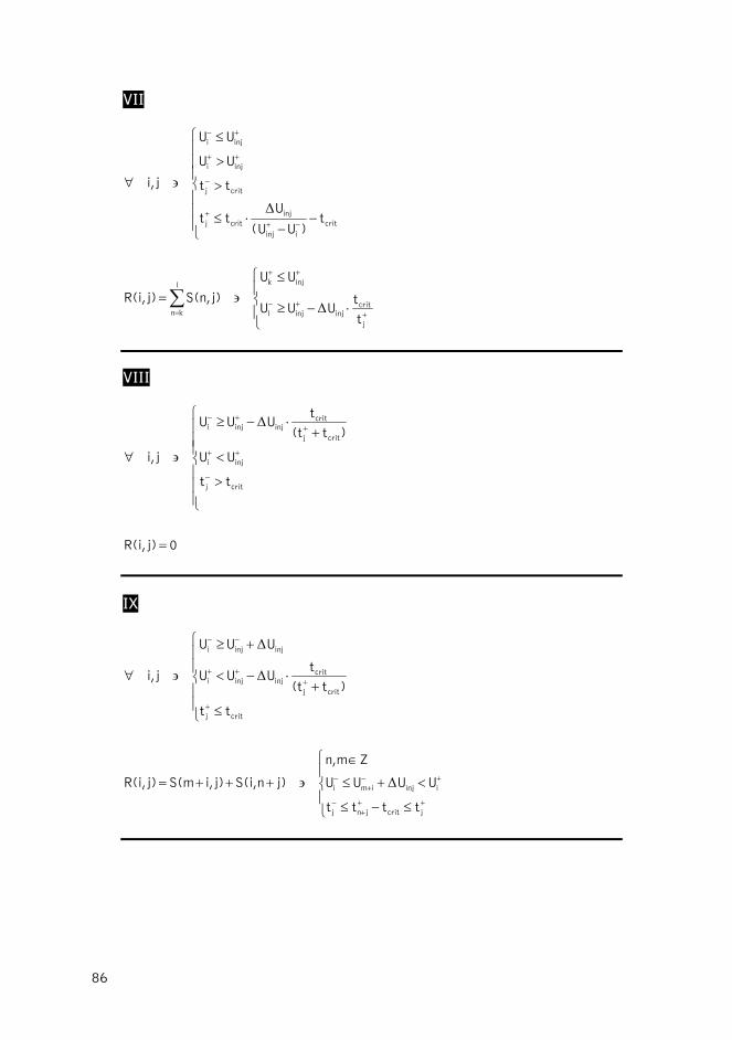
VII
⎪⎩
⎪⎨
⎧
⋅−≥
≤∋=
⎪⎪⎪
⎩
⎪⎪⎪
⎨
⎧
−−
⋅≤
>
>
≤
∋∀
++−
++
=
−++
−
++
+−
∑j
critinjinjl
injkl
kn
critiinj
injcritj
critj
inji
inji
t
tUUU
UU
j)S(n,j)R(i,
t)U(U
Utt
tt
UU
UU
ji,
∆
∆
VIII
0j)R(i,
tt
UU
)t(t
tUUU
ji,
critj
inji
critj
critinjinji
=
⎪⎪⎪
⎩
⎪⎪⎪
⎨
⎧
>
<
+⋅−≥
∋∀−
++
++− ∆
IX
⎪⎩
⎪⎨
⎧
≤−≤
<+≤
∈
∋+++=
⎪⎪
⎩
⎪⎪
⎨
⎧
≤
+⋅−<
+≥
∋∀
+++
−
+−+
−
+
+++
−−
jcritjnj
iinjimi
critj
critj
critinjinji
injinji
tttt
UUUU
Zmn,
j)nS(i,j)i,S(mj)R(i,
tt
)t(t
tUUU
UUU
ji,
∆
∆
∆
86
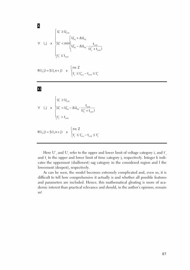
X
⎩⎨⎧
≤−≤
∈∋+=
⎪⎪⎪
⎩
⎪⎪⎪
⎨
⎧
≤
⎪⎩
⎪⎨
⎧
+⋅−
+<
≥
∋∀
+++
−
+
++
−
+
−
jcritjnj
critj
critj
critinjinj
injinj
i
criti
tttt
Znj)nS(i,j)R(i,
tt
)t(t
tUU
UU
minU
UU
ji,∆
∆
XI
⎩⎨⎧
≤−≤
∈∋+=
⎪⎪
⎩
⎪⎪
⎨
⎧
>
+⋅−<
≥
∋∀
+++
−
−
+++
−
jcritjnj
critj
critj
critinjinji
criti
tttt
Znj)nS(i,j)R(i,
tt
)t(t
tUUU
UU
ji, ∆
Here U+i and U-
i refer to the upper and lower limit of voltage category i, and t+j
t-j to the upper and lower limit of time category j, respectively. Integer k indi-
rmost (shallowest) sag category in the considered region and l the lowermost (deepest), respectively.
As can be seen, the model becomes extremely complicated and, even so, it is difficult to tell how comprehensive it actually is and whether all possible features and parameters are included. Hence, this mathematical gloating is more of aca-demic interest than practical relevance and should, in the author’s opinion, remain so!
andcates the uppe
87


ISBN 951-22-6398-X
ISSN 1458-9249


![J.Lund´enandV.Koivunen, “Automaticradarwaveformrecognition ...lib.tkk.fi/Diss/2009/isbn9789522480545/article8.pdf · recognition of communication signals, e.g., [5]–[7]. Automatic](https://img.dokumen.tips/doc/110x75/5f85c66b4ae7a045744098d4/jlund-aoeautomaticradarwaveformrecognition-libtkkfidiss2009isbn9789522480545article8pdf.jpg)