Embed Size (px)
Citation preview

Imperial College London
Department of Computing
ProbPoly - A Probabilistic Inductive Logic Programming
Framework
with Application in Learning Requirements
by
Calin-Rares Turliuc
Submitted in partial fulfilment of the requirements for the MSc Degree inComputing Science / Artificial Intelligence of Imperial College London
September 2011


Acknowledgements
I would like to thank my supervisor Dr. Alessandra Russo for her continuous assistanceand support, for long, challenging and inspiring discussions, and for invaluable feedback andevaluation of my work.
I would also like to thank my second marker Dr. Krysia Broda for an excellent collabo-ration for my ISO project and incommensurable help and advice.
I am thankful for the edifying meetings and unconditional aid of Dalal Alrajeh andDomenico Corapi.
On a personal note, I am grateful for the discussions with Alexandru Marinescu and hissuggestions, and immensely indebted for my parents’ love and financial support.
Abstract
The focus of this project has been on developing a novel Probabilistic Inductive LogicProgramming Framework (PILP) called ProbPoly. The methodology is based on the se-mantics of Stochastic Logic Programs (SLPs), and by using probabilistic examples and anadequate score function to learn probabilities of clauses. Many limitations of existing learn-ing methods for SLPs are overcome, such as non-recursiveness. We also offer a naturalextension for incorporating negation as failure, as well as for learning multiple clauses. Ourrepresentation of predicted probabilities of examples is a (multivariate) polynomial, whoseconstrained minimization ensures that the predicted probabilities are close to the observedones. The minimization task is performed using specific mathematical techniques of relax-ation, and in case we can’t ensure a global optimum, we use a state-of-the-art metaheuristic– particle swarm optimization.
PILP has been successfully applied in numerous areas of research, such as bioinformaticsand natural language processing. We aim to apply it in a software engineering context, withthe purpose of learning requirements. We review related systems, and show how we can useProbPoly in conjunction with the PRISM probabilistic model checker to learn probabilitiesof a simple discrete time Markov chain, such that the new model satisfies a list of properties.To our knowledge, an experiment of learning requirements involving PILP and probabilisticmodel checking has never been done before.
Our conclusions are that ProbPoly is a promising idea for PILP, with a well founded the-oretical background, and spanning numerous directions for improvement, both in theoreticaland technical aspects.

Contents
1 Introduction 1
2 Background 2
2.1 Logic and Logic Programming . . . . . . . . . . . . . . . . . . . . . . . . . . . . . . . 2
2.2 Inductive Logic Programming and Probabilistic ILP . . . . . . . . . . . . . . . . . . 3
2.3 Distribution Semantics . . . . . . . . . . . . . . . . . . . . . . . . . . . . . . . . . . . 4
2.4 Stochastic Logic Programs and Their Semantics . . . . . . . . . . . . . . . . . . . . . 6
2.5 Polynomials . . . . . . . . . . . . . . . . . . . . . . . . . . . . . . . . . . . . . . . . . 9
I ProbPoly - a new PILP framework 12
3 Related Work in (Probabilistic) Inductive Logic Programming 13
3.1 TopLog . . . . . . . . . . . . . . . . . . . . . . . . . . . . . . . . . . . . . . . . . . . 13
3.1.1 Top Directed Hypothesis Derivation . . . . . . . . . . . . . . . . . . . . . . . 13
3.1.2 Mode Declariations and Hypothesis Generation . . . . . . . . . . . . . . . . . 13
3.1.3 Obtaining a Final Theory . . . . . . . . . . . . . . . . . . . . . . . . . . . . . 15
3.2 Stochastic Logic Program Learning . . . . . . . . . . . . . . . . . . . . . . . . . . . . 16
3.3 ProbFOIL - a PILP system in ProbLog . . . . . . . . . . . . . . . . . . . . . . . . . 17
3.3.1 ProbLog . . . . . . . . . . . . . . . . . . . . . . . . . . . . . . . . . . . . . . . 17
3.3.2 ProbFOIL . . . . . . . . . . . . . . . . . . . . . . . . . . . . . . . . . . . . . . 19
4 ProbPoly 21
4.1 A Simple Score for Probabilistic Facts in TopLog . . . . . . . . . . . . . . . . . . . . 21
4.2 A Probabilistic Hypothesis Interpreter . . . . . . . . . . . . . . . . . . . . . . . . . . 22
4.3 Learning SLPs in ProbPoly . . . . . . . . . . . . . . . . . . . . . . . . . . . . . . . . 25
4.3.1 Non-recursive SLPs . . . . . . . . . . . . . . . . . . . . . . . . . . . . . . . . 26
4.3.2 Recursive SLPs . . . . . . . . . . . . . . . . . . . . . . . . . . . . . . . . . . . 28
4.3.3 Negation as Failure . . . . . . . . . . . . . . . . . . . . . . . . . . . . . . . . . 30
4.3.4 Multiple Clauses . . . . . . . . . . . . . . . . . . . . . . . . . . . . . . . . . . 31
4.3.5 True/False Positive/Negatives in SLPs . . . . . . . . . . . . . . . . . . . . . . 34
4.4 Conclusions . . . . . . . . . . . . . . . . . . . . . . . . . . . . . . . . . . . . . . . . . 34
5 Implementation 35
5.1 The MatLab Package Interface . . . . . . . . . . . . . . . . . . . . . . . . . . . . . . 35
5.2 PSOpt . . . . . . . . . . . . . . . . . . . . . . . . . . . . . . . . . . . . . . . . . . . . 35
5.3 Architecture . . . . . . . . . . . . . . . . . . . . . . . . . . . . . . . . . . . . . . . . . 36
5.4 The Impact of Negation as Failure . . . . . . . . . . . . . . . . . . . . . . . . . . . . 37
II Towards Learning Probabilistic Requirements 38
6 Related Work in Learning Requirements 39
6.1 Learning Requirements using ILP and Model Checking . . . . . . . . . . . . . . . . . 39

CONTENTS
6.2 Connectionist Systems for Learning Requirements . . . . . . . . . . . . . . . . . . . 406.3 Automated Verification of Systems using L* . . . . . . . . . . . . . . . . . . . . . . . 42
6.3.1 The L* Algorithm . . . . . . . . . . . . . . . . . . . . . . . . . . . . . . . . . 426.3.2 The Original Framework . . . . . . . . . . . . . . . . . . . . . . . . . . . . . . 446.3.3 Verification in a Probabilistic Context . . . . . . . . . . . . . . . . . . . . . . 46
6.4 The KAOS framework and related methods . . . . . . . . . . . . . . . . . . . . . . . 466.4.1 Introduction and Inference of Requirements Specifications from Scenarios . . 466.4.2 Conflicts and Obstacles in Goal-Driven Requirements Engineering . . . . . . 486.4.3 LTS synthesis based on End-User Scenarios . . . . . . . . . . . . . . . . . . . 49
6.5 The I* Approach . . . . . . . . . . . . . . . . . . . . . . . . . . . . . . . . . . . . . . 51
7 Modelling and Verification. Probabilistic Model Checking. 527.1 Probabilistic Model Checking. PRISM. . . . . . . . . . . . . . . . . . . . . . . . . . . 527.2 Learning A Simple Discrete Time Markov Chain . . . . . . . . . . . . . . . . . . . . 567.3 Conclusions . . . . . . . . . . . . . . . . . . . . . . . . . . . . . . . . . . . . . . . . . 58
8 Future Work 59
9 Conlcusions 62
A Code Listings 63

Chapter 1
Introduction
Probabilistic Inductive Logic Programming (PILP) is a prominent area of research which aimsto combine the expressiveness of learning clauses in a first-order logic language with the uncertaintyof real-world data, quantified by probabilities. PILP has been successfully used in bioinformaticsand natural language processing, and still presents many challenges for researchers interested inprobabilities, logic and machine learning.
Probabilities have also been introduced in the verification of systems. The development ofprobabilistic model checkers, which verify probabilistic properties for probabilistic models such asMarkov chains, has opened the possibility of designing new methods which learn requirements in aprobabilistic setting.
The main contribution of our thesis is the creation of an original framework for PILP. Wecombine elements from Stochastic Logic Program (SLP) learning, which has been studied only fornon-recursive programs and non-probabilistic positive examples, and learners based on distributionsemantics, which use probabilistic examples. The aim of such learners is to learn probabilitiesand/or rules which satisfy certain criteria defined using the probabilities in the background knowl-edge and of the examples.
The merits of our framework are that it allows learning on SLPs with probabilistic exampleswith recursive programs, which is a significant improvement. We further extend our methodologyto include negation as failure, as well as learning probabilities for multiple clauses simultaneously.We also reason about negative examples in the context of SLPs and about various quantitativemeasures used in information retrieval - true/false positives/negatives, and adapted to SLPs.
The main challenge of our approach for learning probabilities will be the constrained minimiza-tion of a multivariate polynomial, a problem overcome by using two state-of-the-art methods. Inthe case of non-recursive programs or when learning a single clause for a recursive program, wefind the probabilities using the analytical method of gradient descent. In the multivariate case,initially we try to find a global minimum using a tool called GloptiPoly, designed specifically foroptimization of polynomial functions. If we don’t succeed, we fall back on the clever metaheuris-tic of Particle Swarm Optimization, which is believed to converge faster than other methods ofevolutionary computation.
In the second part of our thesis we analyse the possibility of using PILP in conjunction witha probabilistic model checker in order to learn new probabilities of an initial model, such that theproperties which are not satisfied in the initial are valid in the new model. An experiment is carriedout on a simple model and proves successful.
Finally we identify the possible directions of future research, which include extending the learn-ing of SLPs to multiple predicates, learning with proofs of infinite length, and combining ourmethod with an ILP system to in order to interleave the process of learning the logical clauses withthat of learning their associated probabilities.
1

Chapter 2
Background
This chapter will introduce elementary concepts from different areas of mathematics, logic andcomputer science, which are necessary for the understanding of the rest of the thesis. Since themain contribution is a probabilistic inductive logic programming framework, we begin our discussionwith the topics of logic and logic programming in Section 2.1, and learning using logic: inductivelogic programming and probabilistic inductive logic programming in Section 2.2. As we shall see,probabilistic inductive logic programming is a paradigm in which the definition of probabilities withrespect to logic programming has a crucial impact. We treat two of perhaps the most popular viewson semantics of probabilities: distribution semantics in Section 2.3 and stochastic logic programsin Section 2.4. We will adopt the latter in our novel framework.
Finally, our framework relies on the manipulation and, most importantly, the constrained op-timization of (multivariate) polynomials, so we introduce relevant aspects of such fundamentalmathematical expressions in Section 2.5.
2.1 Logic and Logic Programming
We assume familiarity with the syntax and semantics of propositional and first-order logic,unification and resolution. We also assume knowledge about Linear Temporal Logic (LTL), whichextends first-order logic with operators for temporal sequences; however, we will explain intuitivelythe required operators when they are introduced. We also assume knowledge of the Prolog notation,which we will use throughout the thesis (atoms and predicates start with lower-case letters, variablesstart with upper-case letters, we use ”:-” with the same meaning as logical ”←”). In the remainderof the section we introduce in a semi-formal manner a minimal amount of concepts from first-orderlogic and logic programming. The presentation is inspired by the first part (especially chapters 2and 7) of [Nienhuys-Cheng and Wolf, 1997], which deals with these matters formally and at length.
A predicate is also called an atom, or, when referring to logic programming, a goal, and can beassigned truth values (true or false).
A literal is an atom or a negated atom. Usual operations on literals include conjunction (∧),disjunction (∨), negation (¬), implication (→, and its inverse, the conditional ← ) and equivalence(↔).
A clause is a disjunction of literals (l1 ∨ l2...∨ ln). An empty clause is denoted by [ ] or �, andits truth value is false.
A Horn clause C is a clause with at most one positive literal. It will be written in the formq ← l1, ..., ln with n ≥ 0, where q is an atom and all li with 1 ≤ i ≤ n are atomic literals, and q,or C+, is called the head and l1, . . . , ln, or C−, is called the body of the clause. Clause bodies areunderstood to be conjunctions of literals.
If all li are atoms a clause is called definite. If we allow negation, i.e. li = not A, where A is anatom, a clause is called normal. A denial clause is a clause of the form ← l1, . . . , ln. The numberof literals in the body of a clause is called the length of the clause.
A (normal logic) program P is a finite set of (normal) clauses and a definite logic program is afinite set of definite clauses.
2

2.2 Inductive Logic Programming and Probabilistic ILP
An interpretation maps predicates to true or false. We will usually identify an interpretationwith the set of predicates which it maps to true (the rest are implicitly assumed to be false). Aninterpretation is extended to literals, clauses and programs in the usual way.
A model of a clause C is an interpretation I which maps C to true (in symbols: I C). Amodel of a program P is an interpretation which maps every clause in P to true.
Let Σ be a set of Horn clauses, and C be a Horn clause. An SLD-derivation of length k of Cfrom Σ is a finite sequence of Horn clauses R0, . . . , Rk, and Rk = C, such that R0 ∈ Σ and eachRi, i = 1, k, is a binary resolvent of Ri−1 and a definite program clause Ci ∈ Σ, using the head ofCi and a selected atom in the body of Ri−1 as the literals resolved upon.
An SLD-derivation of the empty clause [ ] from Σ is called an SLD-refutation of Σ. A goal is aclause.
Let P be a definite program, and G a definite clause. An SLD-tree for P ∪ {G} is a treesatisfying the following:
� Each node of the tree is a (possibly empty) definite goal.
� The root node is G.
� Let N =← A1, . . . , As, . . . , Ak, k ≥ 1, be a node in the tree, with As as selected atom. Then,for each clause C in P such that As and (a variant of) C+ are unifiable, the node N hasexactly one resolvent of N and C, Bs, as a child. The node has no other children for thesame As and C.
� Nodes which are the empty clause [ ] have no children.
Negation as Failure (NaF) is a method that allows us to introduce negated atoms, and thusworking with normal logic programs rather than definite logic programs. The essential idea is thatfor a definite goal G, we assume that ¬G is proven if G finitely fails. Let P be a definite program,an SLD-tree for P ∪ {G} is called finitely failed if it is finite and contains no success branches.
SLD-resolution that takes into account negation as failure is called SLDNF-resolution, which isthe standard resolution technique used in logic programming. However, we will leave out all thetechnical details about SLDNF-trees and SLDNF-resolution, because they are beyond the scope ofthis thesis.
2.2 Inductive Logic Programming and Probabilistic ILP
Inductive Logic Programming (ILP) is a field related to Logic, Logic Programming and MachineLearning, which aims at learning a (normal logic) program, referred to as theory or hypothesis H,based on domain knowledge, encoded as background knowledge, language bias, which is essentialto reduce the search space, especially when learning complex predicates, and a set of positive andnegative examples, the quality of which is crucial to the success of the learning.
The usual setting of ILP, as defined in [Nienhuys-Cheng and Wolf, 1997], is: given a set ofclauses B (background knowledge) and sets of clauses E+ and E− (positive and negative examples),find a theory (i.e. a set of clauses) H such that H ∪B is correct with respect to E+ and E−, whichwe will denote by H ∪B |= E. A set of clauses P is correct with respect to positive examples E+
if: P |= e, ∀e ∈ E+. A set of clauses P is correct with respect to negative examples E− if: P 2 e,∀e ∈ E−. It can be proven that we can transform examples into ground examples, since we makethe Closed World Assumption (CWA), that is, everything which is not asserted to be true by ourprogram is implicitly false.
As an example, consider:B = { parent(bob, alan), parent(mia, kate),
male(bob),male(alan),female(mia), female(kate)},
and examples E+ = {has daughter(mia)} and E− = {has daughter(bob)}.Furthermore, assume H = {has daughter(X) ← parent(X,Y ), female(Y )}. This is the in-
tuitive ”human” definition of the has daughter predicate, and in this case H ∪ B |= E. Now
3

2. BACKGROUND
let us make H = {has daughter(X) ← parent(X,Y )}, which would correspond to the ”in-tuitive” has children predicate, then H ∪ B 2 E, because H ∪ B |= has daughter(bob), andhas daughter(bob) ∈ E−. Finally, we may learn a theory such as H = {has daughter(X) ←parent(X,Y ), female(X)}, which again corresponds to the ”intuitive” is mother predicate, butwe have H ∪ B |= E, so the learned theory is ”correct”. This can be seen as an ILP case ofoverfitting, and as mentioned earlier, we must have either an intuition about the predicate we wantto learn, to generate appropriate examples, or have an oracle generate a large number of examples,to precisely guide the search towards the correct theory.
We also mention the task of abductive logic programming ([Kakas et al., 1993]). An ALP task,as defined in [Corapi et al., 2010], is based on 〈g, T,A, I〉, where g is a ground goal, T is a normallogic program, A is a set of ground facts called abducibles, and I is a set of denial clauses calledintegrity constraints. The output of the abductive procedure is a subset of A, called abductivesolution – ∆, such that T ∪∆ is consistent, T ∪∆ |= g and T ∪∆ |= I.
Probabilistic Inductive Logic Programming (PILP) is a branch of ILP which aims at combiningthe expressiveness of inductive logic learning with probabilistic reasoning, motivated by the uncer-tainty inherent in data. An excellent review can be found in [Raedt and Thon, 2010], which distin-guishes between learning from entailment, interpretations and proofs, and proposes an adaptationof FOIL [Quinlan and Cameron-Jones, 1993] for probabilistic learning from entailment. However,unlike ILP, there is no general consensus as to what the task of PILP should be. This is due tothe various semantics of probabilities in logic programming. We will overview two perspectives onthe semantics of probabilities in Sections 2.3 (Distribution Semantics) and 2.4 (Stochastic LogicPrograms Semantics).
2.3 Distribution Semantics
It is fundamental for PILP to have a theoretically founded semantics. Sato’s distribution se-mantics, introduced in [Sato, 1995], assigns a probability for each formula over an infinite Herbranduniverse, such that the probability axioms of Kolmogorov hold. The three axioms are:
1. Any probability is a non-negative real number.
2. The probability of an elementary event to occur over a sample space is 1. Intuitively, thismeans that we take into consideration all possible events in the sample space.
3. In the case of pairwise disjoint events, the probability of all the events is the sum of theprobabilities of the individual events.
Sato considers definite clause programs DB of the form: DB = F ∪ R, where F is the set offacts, and R is the set of rules. The key idea is to initially define a probability distribution over F ,PF , and to extend it over the whole program DB, thus obtaining PDB, in a process influenced bythe set of rules R. DB is assumed to be ground, denumerably infinite, and satisfying the disjointcondition, i.e. no fact in F unifies with the head of a rule in R.
Assume that A1, A2, . . . , An are atoms in F , P(n)F is the joint probability over the first n variables
in F , i.e. A1, A2, . . . , An, and that x1, x2, . . . , xn are 0 or 1 (corresponding to false or true, i.e.Ai = 1 means that atom Ai is true in the current interpretation). The existence of PF is provedby ensuring that the following conditions hold:
1. 0 ≤ P (n)F (A1 = x1, A2 = x2, . . . , An = xn) ≤ 1
2.∑
x1,x2,...,xn
P(n)F (A1 = x1, A2 = x2, . . . , An = xn) = 1
3.∑xn+1
P(n+1)F (A1 = x1, A2 = x2, . . . , An+1 = xn+1) = P
(n)F (A1 = x1, A2 = x2, . . . , An = xn)
4

2.3 Distribution Semantics
The first condition ensures that the values of the probabilities defined are valid. The secondcondition is motivated by the need of completeness of the sample space (in this case, the proba-bilities over all interpretations must sum up to 1). The third condition, called the compatibilitycondition defines an additive property of probabilities, and is related to the completeness problem(an interpretation must be either true or false, so marginalizing over these two possibilities mustsum up to 1).
The probability PDB is constructed from PF by considering all the interpretations I for which,their least models (LM(I)) logically imply the atoms in F . PDB is then defined as PF over the setof such interpretations:
[Ax11 ∧ Ax22 ∧ · · · ∧ Axnn ]F
def= {I | LM(I) |= (Ax11 ∧ A
x22 ∧ · · · ∧ Axnn )} , where Axii is A if xi = 1
or ¬A if xi = 0.The formal definition of PDB is:
P(n)DB(A1 = x1, A2 = x2, . . . , An = xn)
def= PF ([Ax11 ∧A
x22 ∧ · · · ∧Axnn ]F )
However, we don’t know how to compute a probability over a set of interpretations. Proposition2.1 from [Sato, 1995] provides an answer to this problem. Let:
ϕDB(x1, x2, . . . , xn) =< y1, y2, . . . , yk > iff∀I (I |= A1, . . . , An → LM(I) |= B1, . . . , Bk)Then the whole distribution is:PDB(A1, . . . , An, B1, . . . , Bk) ={
PF (A1, . . . , An) if ϕDB(x1, x2, . . . , xn) =< y1, y2, . . . , yk >
0 otherwise
The intuition behind this definition is that the probabilities of the interpretations over DBshould be in fact the probabilities of the interpretations over F , but taking care that the rest of theatoms in the interpretations over DB should be assigned the correct values (obtained by inductionof these atoms using the interpretations over F and the rules R).
The distribution over the head atoms is computed by summing (or marginalizing) over theprobabilities of the interpretations that are consistent with B1, . . . , Bk:
PDB(B1, . . . , Bk) =∑
ϕDB(x1,x2,...,xn)=<y1,y2,...,yk>
PF (A1, . . . , An)
The easiest way to understand distribution semantics is via an example.
Example 2.1. Let DB = F ∪R, F = {X,Y },and R = { A← X,
B ← X,B ← Y ,C ← X,Y }
Assume PF is defined as:
〈xX , xY 〉 PF (xX , xY )
〈0, 0〉 0.2
〈1, 0〉 0.4
〈0, 1〉 0.1
〈1, 1〉 0.3
others 0
Then, PDB will be:
〈xX , xY , xA, xB, xC〉 PDB(xX , xY , xA, xB, xC)
〈0, 0, 0, 0, 0〉 0.2
〈1, 0, 1, 1, 0〉 0.4
〈0, 1, 0, 1, 0〉 0.1
〈1, 1, 1, 1, 1〉 0.3
others 0
5

2. BACKGROUND
Suppose we now want to compute PDB(A = 1). This reduces to a simple marginalization overPF (xX , xY , xA, xB, xC):
PDB(A = 1) = PDB(1, 0, 1, 1, 0) + PDB(1, 1, 1, 1, 1) = 0.7
In the same way:
PDB(B = 1) = PDB(1, 0, 1, 1, 0) + PDB(0, 1, 0, 1, 0) + PDB(1, 1, 1, 1, 1) = 0.8
Finally, we mention a probabilistic logic programming language called PRogramming In Statis-tical Modelling (PRISM1) described in [Sato and Kameya, 2001]. In this language we can specifylogic programs which simulate the behaviour of Turing Machines, Bayes Networks, Markov Chains(e.g. Hidden Markov Models (HMMs)) etc. The authors also design an Expectation Maximization(EM) algorithm to evaluate P (A1, ..., An) if we know P (B1, ..., Bk), and which subsumes the specificversion of EM for different models.
2.4 Stochastic Logic Programs and Their Semantics
Stochastic Logic Programs are introduced in [Muggleton, 1996], as a way to represent Stochastic(or Probabilistic) Context Free Grammars (SCFG or PCFG) in logic programming, and are definedas a set of stochastic clauses. A stochastic clause p : C is a pair of a probability p ∈ [0, 1] and arange-restricted clause C. A clause is range-restricted if every variable in the head of C is foundin the body. Moreover, the set of stochastic clauses must satisfy the property that for all clausescontaining q as the predicate of the head, the probabilities of these clauses must sum up to 1. Itis easy to transform any logic program consisting of only range-restricted clauses annotated withprobabilities into a SLP by normalization.
A Stochastic SLD (SSLD) refutation consists of the SLD refutation of the logic program (ig-noring probabilities). Then, the probability of a derivation of a goal g is defined as the productof probabilities on the branches of the SLD tree, and the probability of goal g is the sum of theprobabilities of all the derivations of g. Formally, we have:
Definition 2.1 (The Probability of a Derivation of a Goal). The probability of a derivation (in asuccessful case called a proof or refutation) proof of a goal g (given background knowledge B andhypothesis H) is :
P (g|B ∪H, proof) =∏
p:c∈proofp
Definition 2.2 (The (Total) Probability of a Goal). The total probability of a goal g (given back-ground knowledge B and hypothesis H) is :
P (g|B ∪H) =∑
proof∈SSLD(g,B∪H)
P (g|B ∪H, proof)
=∑
proof∈SSLD(g,B∪H)
∏p:c∈proof
p
Consider the following example from [Chen et al., 2008]:
Example 2.2. SSLD derivation of s(X).0.4 : s(X) :- p(X), p(X).0.6 : s(X) :- q(X).
0.3 : p(a).0.7 : p(b).
0.2 : q(a).0.8 : q(b).
1We won’t use the abbreviation due to a name clash with the probabilistic model checker.
6

2.4 Stochastic Logic Programs and Their Semantics
We reproduce the SSLD derivation tree with annotated probabilities in Figure 2.12:
Figure 2.1: Example of SSLD derivation tree.
Notice that there are 6 derivations with 4 refutations and 2 fail-derivations. So, the (total)probability of goal s(X):
P (s(X)) =∑
r∈Refuations(s(X))
P (r)
= 0.4 ∗ 0.3 ∗ 0.3 + 0.4 ∗ 0.7 ∗ 0.7 + 0.6 ∗ 0.2 + 0.6 ∗ 0.8
= 0.036 + 0.196 + 0.12 + 0.48
= 0.832
A nice property is that in the context of SLPs, the probability of all derivations, i.e. refutationsas well as failed derivations, of any goal is 1, due to the fact that for any clauses with the samepredicate in the head, the sum of the annotated probabilities must be 1.
We have mentioned that SLPs were designed for representing Probabilistic Context Free Gram-mars (PCFG) in a logic programming context. Let us define PCFGs formally and then provide asmall example from Natural Language Processing (NLP), inspired by [Manning and Schutze, 1999].
Definition 2.3 (Probabilistic Context Free Grammar). A PCFG G consists of:
� A set of terminals, {wk}, k = 1, . . . , V
� A set of nonterminals, {N i}, i = 1, . . . , n
� A designated start symbol, N1
� A set of rules, {N i → ζj}, (where ζj is a sequence of nonterminals)
� A corresponding set of probabilities on rules such that:
∀i∑j
P (N i → ζj |N i) = 1
Consider the following PCFG3:
Example 2.3. Simple PCFG example.S → NP VP 1.0 NP → NP PP 0.4PP → P NP 1.0 NP → astronomers 0.1VP → V NP 0.7 NP → ears 0.18VP → VP PP 0.3 NP → saw 0.04P → with 1.0 NP → stars 0.18V → saw 1.0 NP → telescopes 0.1
2Figure 1(b) in [Chen et al., 2008].3Table 11.2 from [Manning and Schutze, 1999].
7

2. BACKGROUND
We can directly model this PCFG into an SLP, by just considering probabilistic clauses of theform: 1 : s ← np, vp for the first rule in the PCFG, and so on. When considering (graphical)representations of PCFG we have the following result: for every PCFG there exists an equivalentPushdown Automaton (PDA). However, it is convenient to represent a particular derivation of astring by the grammar using parse trees. Let us consider sentence S = [astronomers, saw, stars,with, ears], which can be parsed in two ways by the grammar in Example 2.3. The parse tree forthe two derivations are shown in Figure 2.2.4
Figure 2.2: The parse trees for sentence [astronomers, saw, stars, with, ears] using the PCFG fromExample 2.3.
The probability of a derivation is the product of all the probabilities in its parse tree, and isequivalent to the probability of a derivation of a goal in Definition 2.1, if we consider the goal tobe the string that is parsed, and the logic program the representation of the grammar. In a similarmanner, the probability of a string being derived by a PCFG is the sum over the probabilities ofall derivations, which is again reflected in the (total) probability of a goal in Defintion 2.2, underthe same circumstances as the ones mentioned above.
Note that this PCFG can in fact be represented in a logic programming language such asProlog, as shown in Listing 2.1.5 However, it is worthy to mention the problem of left recursion,which appears for rules of the form R → R.... If we don’t transform the parsing in an acceptablerecursive paradigm (boundary condition and recursive case), we end up with an infinite loop in theexecution.6 By adequately querying the system after program compilation, we get the expectedparse trees and the correct probabilities, as shown in Listing 2.2.
Listing 2.1: Prolog definition of PCFG in Example 2.3.
0 s ( P0 , s ( NP , VP ) ) −−> np ( P1 , NP ) , vp ( P2 , VP ) , { P0 i s 1 .0* P1*P2 } .
np ( 0 . 1 , np ( astronomers ) ) −−> [ astronomers ] .np ( P0 , np ( astronomers , Rest ) ) −−> [ astronomers ] , nptail ( P1 , Rest ) , {P0 i s P1 *0 . 1} .np ( 0 . 1 8 , np ( ears ) ) −−> [ ears ] .
5 np ( P0 , np ( np ( ears ) , Rest ) ) −−> [ ears ] , nptail ( P1 , Rest ) , {P0 i s P1 *0 . 1 8} .np ( 0 . 0 4 , np ( saw ) ) −−> [ saw ] .np ( P0 , np ( saw , Rest ) ) −−> [ saw ] , nptail ( P1 , Rest ) , {P0 i s P1 *0 . 0 4} .np ( 0 . 1 8 , np ( stars ) ) −−> [ stars ] .np ( P0 , np ( np ( stars ) , Rest ) ) −−> [ stars ] , nptail ( P1 , Rest ) , {P0 i s P1 *0 . 1 8} .
10 nptail ( Acc , np ( NP , PP) ) −−> pp( P2 , PP) , np ( Acc1 , NP ) , {Acc i s 0 .4* P2*Acc1 } .nptail ( Acc , PP) −−> pp( P2 , PP) , {Acc i s 0 .4* P2 } .
4Reproduced from figure 11.1 in [Manning and Schutze, 1999].5The code is inspired by the simpler example at http://w3.msi.vxu.se/~nivre/teaching/statnlp/pdcg.html
(accessed 01.09.2011).6See http://www.cs.sfu.ca/~cameron/Teaching/383/DCG2.html(accessed 01.09.2011) for details and a more ac-
cessible example.
8

2.5 Polynomials
pp( P0 , pp (P , NP ) ) −−> p ( P1 , P ) , np ( P2 , NP ) , {P0 i s 1 .0* P1*P2 } .
15 vp ( P0 , vp (V , NP ) ) −−> v ( P1 , V ) , np ( P2 , NP ) , { P0 i s 0 .7* P1*P2 } .vp ( P0 , vp ( vp (V , NP ) , Rest ) ) −−> v ( P1 , V ) , np ( P2 , NP ) , vtail ( P3 , Rest ) ,{ P0 i s 0 .7* P1*P2*P3 } .vtail ( P0 , PP) −−> pp( P1 , PP) , {P0 i s 0 .3* P1 } .vtail ( P0 , VP ) −−> vp ( P0 , VP ) .
20 p ( 1 . 0 , p ( with ) ) −−> [ with ] .v ( 1 . 0 , v ( saw ) ) −−> [ saw ] .
Listing 2.2: Results of the query to compute the parse trees and their probabilities.
0 ?− s (P , T , [ astronomers , saw , stars , with , ears ] , [ ] ) .P = 0.0009072 ,T = s ( np ( astronomers ) , vp ( v ( saw ) , np ( np ( stars ) , pp ( p ( with ) , np ( ears ) ) ) ) ) ? ;P = 0.0006804 ,T = s ( np ( astronomers ) , vp ( vp ( v ( saw ) , np ( stars ) ) , pp ( p ( with ) , np ( ears ) ) ) ) ? ;
5 no
2.5 Polynomials
Polynomials are fundamental mathematical expressions which use constants and one (in whichcase we shall call them univariate) or more variables (in which case we shall call them multivariate).The constants, as well as the variables, are usually defined over the well known sets: N, Z, R, ormore generally C.
For the moment, assume we discuss univariate polynomials over C. A polynomial of this typeis written as:
p(x) = anxn + an−1x
n−1 + ...+ a1x+ a0, with n ∈ N, x, a0, a1, . . . , an ∈ C and an 6= 0.n is the degree of the polynomial p(x). If n = 0, then the polynomial is a constant function
p(x) = a0. A value x0 is called a root of the polynomial p(x) if p(x0) = 0.
Property 2.1. x0 is a root of p(x) of degree n ≥ 1 i.f.f. there exists polynomial q(x) of degreen− 1 and p(x) = q(x)(x− x0).
The proof of the above property is straightforward:⇐: If we have p(x) = q(x)(x− x0), then p(x0) = 0, so, by definition x0 is a root.⇒: By the remainder theorem, we have: p(x) = q(x)(x− x0) + c, c ∈ C. However, x0 is a root,
so p(x0) = c = 0.
Theorem 2.1 (Fundamental Theorem of Algebra). Let p(x) be a polynomial of degree n ≥ 1.Then, p(x) always has a root x0 ∈ C.
By using the fundamental theorem of algebra, and Property 2.1, we can inductively prove thefollowing result:
Property 2.2. Let p(x) be a polynomial of degree n ≥ 1. Then, p(x) has at most n complex roots.
The reason why we use ”at most” and not ”exactly” is due to multiple roots, e.g. p(x) = (x−1)2,with root 1 being a multiple root (of order 2).
Among the many observations that can be made about polynomials, we shall mention mainlythe following:
� if p(x) has root x0 = a+ ib, then the complex conjugate of x0, x0, is also a root. Informally,complex roots come in pairs.
� the derivative of a polynomial p(x) of degree n ≥ 1 is a polynomial q(x) of degree n− 1.
� there exist efficient algorithms to determine the real roots of polynomials, among the mostrecent being [Rouillier and Zimmermann, 2004].
9

2. BACKGROUND
� we can find the minimum (or maximum) of a polynomial p(x) in an interval [a, b], by inspectingthe real roots of the derivative in [a, b], which are either local maxima or minima, and thevalues of p(a) and p(b), and keeping the minimum (or maximum).
We will also use multivariate polynomials, which have the general form:
p(x1, ..., xk) =
n∑i=0
aixp(1,i)1 x
p(2,i)2 . . . x
p(k,i)k , with n ∈ N, k ∈ N∗,
ai ∈ C, ∀i = 0, n,
xj ∈ C, ∀j = 1, k, and
p(j, i) ∈ N, ∀i = 0, n,∀j = 1, k
The degree of a multivariate polynomial is maxi
k∑j=1
p(j, i), and a root is a vector [x01, ..., x0k] such
that p(x01, ..., x0k) = 0.
The problem of finding the roots of a multivariate polynomial or of minimizing a multivariatepolynomial (eventually, under certain constraints) is a difficult task in general. In some cases, theroots of multivariate polynomials can be found using Grobner bases. The problem of solving setsof multivariate equations has been given attention due to the development of multivariate publickey cryptography, which was motivated by the fact that quantum computers can perform integerfactorization in polynomial time, and potentially break (univariate) public key cryptosystems suchas the commonly used RSA.7
To minimize a multivariate polynomial under constraints, we use a special numerical method,implemented in MatLab, called GloptiPoly ([Henrion and Lasserre, 2002], [Henrion et al., 2007]).However, since it is not always reliable, and it is scalable only up to a certain extent, we canalso treat this problem as a general function optimization problem, and use metaheuristics such assimulated annealing, genetic algorithms, ant colony optimization or particle swarm optimization.The disadvantage of metaheuristics is that we lose the guarantee of a global minimum, and thecomputation can be just as, or even more expensive.
To give an example, one of the well known functions used to test minimization problems is theSix Hump Camel Back function8, which is a multivariate polynomial of 2 variables and of degree6, given in Listing 2.3.
Listing 2.3: MatLab Definition of Six Hump Camel Back Function
0 f unc t i on [ out ] = sixhump ( x )out = (4−2.1*x (1)ˆ2+x (1)ˆ4/3)* x (1)ˆ2+x (1)* x(2)+(−4+4*x (2 )ˆ2)* x ( 2 ) ˆ 2 ;end
If we consider the constraints: −2 ≤ x1 ≤ 2 and −1 ≤ x2 ≤ 1, then the function has twoglobal minima ( and 4 local minima), f(x1, x2) = −1.0316, for (x1, x2) = (−0.0898, 0.7126), or(0.0898,−0.7126). We illustrate the function in Figure 2.3. The two dark blue valleys correspondto the two global minima.
7See [Ding et al., 2006] for details.8For example, it is mentioned in the GEATbx MatLab toolbox ( http://www.geatbx.com/docu/fcnindex-01.
html (accessed 01.09.2011) ).
10

2.5 Polynomials
Figure 2.3: Plot of the Six Hump Camel Back Function.
Finally, we mention two theorems which allow us to compute polynomials raised to a power.
Theorem 2.2 (Binomial Theorem). The expansion of (x + y)n is: (x + y)n = C(n, 0)xny0 +C(n, 1)xn−1y1 + · · ·+ C(n, n− 1)x1yn−1 + C(n, n)x0yn, with x, y ∈ R, and n ∈ N∗
C(n, k) are binomial coefficients, and:C(n, k) = n!
k!(n−k)! , n ∈ N∗, and 0 ≤ k ≤ nA more general result is the multinomial theorem.
Theorem 2.3 (Multinomial Theorem). The expansion of (x1 +x2 + · · ·+xm)n is: (x1 +x2 + · · ·+
xm)n =∑
k1+k2+···+km=n
(C(n; k1, k2, . . . , km)m∏t=1
xktt )
C(n; k1, k2, . . . , km) are multinomial coefficients, and:C(n; k1, k2, . . . , km) = n!
k1!k2!...km!Note that for binomial and multinomial coefficients although we give the usual definitions based
on the factorials, the implementation uses very fast MatLab functions.
11

Part I
ProbPoly - a new PILP framework
12

Chapter 3
Related Work in (Probabilistic)Inductive Logic Programming
This chapter presents the (P)ILP frameworks which have inspired us to develop ProbPoly. InSection 3.1 we briefly introduce the idea of top directed hypothesis derivation, illustrated by TopLog.In the next chapter, we will adapt the TopLog scoring using probabilistic facts and examples, basedon SLP semantics. In Section 3.2 we continue the discussion on SLPs, introduced in Section 2.4,with an emphasis on learning SLPs, which is also the main goal of ProbPoly. Finally, Section3.3 succinctly describes a popular probabilistic logic programming language, ProbLog, based ondistribution semantics, introduced in Section 2.3, and ProbFOIL, a PILP system implemented inProbLog, based on the ILP FOIL system [Quinlan and Cameron-Jones, 1993].
3.1 TopLog
3.1.1 Top Directed Hypothesis Derivation
TopLog is an Inductive Logic Programming system which illustrates the theoretical frameworkof Top-Directed Hypothesis Derivation (TDHD), described in [Muggleton et al., 2008]. The keyidea of TDHD is to build a top theory > from the background knowledge and based on a set ofnon-terminal symbols NT . The predicates in NT must be new predicates, different from the onesin the background knowledge B. The top theory > is a general logic program from which thehypotheses H is be derived. > must contain as the head of the first clause the target predicate,and as heads of the other clauses in >, non terminal symbols in NT .
We reproduce Example 1 from [Muggleton et al., 2008]. Let:
NT = {ntBody}B = b1 = pet(lassy)←e = nice(lassy)←
Then, > could be written as:
>1 : nice(X)← ntBody(X)
>2 : ntBody(X)← pet(X)
>3 : ntBody(X)← friend(X)
3.1.2 Mode Declariations and Hypothesis Generation
The top theory can also be constructed from mode declarations.
13

3. RELATED WORK IN (PROBABILISTIC) INDUCTIVE LOGICPROGRAMMING
Definition 3.1 (Mode Declaration). A mode declaration, as defined in [Corapi et al., 2010], iseither a head (modeh(s)) or a body declaration (modeb(s)), where s is called a schema, which isa ground literal containing placemarkers. Placemarkers are either inputs (+type), outputs(−type),or ground terms (#type).
Consider the following example1:
Example 3.1. Learning the uncle predicate.B = {
b1 : male(tom)b2 : male(bob)
b3 : parent(tom, mary)b4 : parent(tom, bob)b5 : parent(tom, betty)b6 : parent(mary, ann)b7 : parent(joyce, susan)
}E = {
ID Example clause Example weight
e1 : uncle(bob, ann) +10e2 : uncle(bob, susan) −10e3 : uncle(betty, ann) −10e4 : uncle(tom, betty) −10e5 : uncle(joyce, ann) −10e6 : uncle(tom, mary) −10
}
Assume the following mode declarations:M = {
modeh(uncle(+person))modeb(male(+person))modeb(parent(+person, -person))modeb(parent(-person, +person))
}We might build > as :> = {
>1 : uncle(X,Y )← ntBody(X), ntBody(Y )>2 : ntBody(X)←>3 : ntBody(X)← male(X), ntBody(X)>4 : ntBody(X)← parent(X,Z), ntBody(X), ntBody(Z)>5 : ntBody(X)← parent(Z,X), ntBody(X), ntBody(Z)
}Once we have built >, the generation of the hypotheses set H is based on iterating on the
positive examples E+: starting with H = ∅ for each positive example e ∈ E+, we consider therefutations r of e using B and >, and based on the refutations we build the hypotheses He andmerge them with H.
For the above example, we may have many hypotheses hi ∈ H, such as:
h1 : uncle(X,Y ).
(not(uncle(bob, ann)),>1, | >2, | >2)
h2 : uncle(X,Y ) :- male(X).
(not(uncle(bob, ann)),>1, | >3, b2,>2, | >2)
h3 : uncle(X,Y ) :- parent(Z,X).
1For the examples, a positive weight denotes a positive example, and a negative one – a negative example.
14

3.1 TopLog
(not(uncle(bob, ann)),>1, | >5, b4,>2,>2, | >2)
h4 : uncle(X,Y ) :- parent(Z.Y ).
(not(uncle(bob, ann)),>1, | >2, | >5, b6,>2,>2)
. . .
In brackets we show the corresponding derivation of the (only) positive example e1. We haveused | to mark the beginning of the refutations for each argument of >1. Notice that for examplethe hypothesis uncle(X,Y ) :- parent(X,Z). cannot be generated, since bob isn’t anyone’s parent inB. Now let us consider more complex hypotheses, among which we will find the ”correct” definitionof the uncle predicate (h7):
. . .
h5 : uncle(X,Y ) :- male(X), parent(Z, Y ).
(not(uncle(bob, ann)),>1, | >3, b2,>2, | >5, b6,>2,>2)
h6 : uncle(X,Y ) :- male(X), parent(Z1, X), parent(Z2, Y ).
(not(uncle(bob, ann)),>1, | >3, b2,>5, b4,>2,>2| >5, b6,>2,>2)
h7 : uncle(X,Y ) :- male(X), parent(Z1, X), parent(Z1, Z2), parent(Z2, Y ).
(not(uncle(bob, ann)),>1, | >3, b2,>5, b4,>2,>4, b3,>2,>4, b6,>2,>2| >2)
h8 : uncle(X,Y ) :- parent(Z1, X), parent(Z1, Z2), parent(Z2, Y ).
(not(uncle(bob, ann)),>1, | >3,>5, b4,>2,>4, b3,>2,>4, b6,>2,>2| >2)
. . .
3.1.3 Obtaining a Final Theory
After the generation of all hypotheses, the TopLog system computes the final theory T , whichis a subset of the derived hypotheses H. Initially, T is empty, and hypotheses from H are addedaccording to a greedy heuristic, more specifically at each iteration hypothesis h ∈ H is added to Tif it gives the maximum score of T ∪ h (relative to the other existing hypotheses). The score of Tis computed as:
S(T ) =∑
e∈ECT
weight(e)−∑h∈T|h|
We use ECT to denote the set of examples covered by the hypotheses in T , and by weight(e)the weight of an examples (a positive value for a positive example and a negative value otherwise).|h| is the number of literals in hypothesis h. Thus, the two components of the score account forthe maximization of the weights of the examples (the first sum), while penalizing complex rules(the second sum), which is an ILP way of implementing the Minimum Description Length (MDL)principle.
Again, consider the example of hypotheses h5–h8, and assume T = ∅. We compute the followingscores, for weight(e) = 10 for a positive example and −10 otherwise:
S(T ∪ h5) =
e1︷︸︸︷10 +
e2︷ ︸︸ ︷(−10) +
e4︷ ︸︸ ︷(−10) +
e6︷ ︸︸ ︷(−10)−
# literals︷︸︸︷3 = −23
S(T ∪ h6) =
e1︷︸︸︷10 +
e2︷ ︸︸ ︷(−10)−
# literals︷︸︸︷4 = −4
S(T ∪ h7) =
e1︷︸︸︷10 −
# literals︷︸︸︷5 = 5
S(T ∪ h8) =
e1︷︸︸︷10 +
e3︷ ︸︸ ︷(−10)−
# literals︷︸︸︷4 = −4
It is clear that in the first iteration we will add h7 to T . Also, since every other hypothesis willcontribute a negative score, we can anticipate that in the second iteration no hypothesis will beadded to T and the final theory will be T = {h7}, as we would expect.
15

3. RELATED WORK IN (PROBABILISTIC) INDUCTIVE LOGICPROGRAMMING
3.2 Stochastic Logic Program Learning
The problem of learning probabilities of an SLP is addressed in [Muggleton, 2002]. We mustlearn a set of probabilistic clauses H such that the SLP S = B∪H |= E (B is also an SLP and E isa set of ground positive non-probabilistic examples). Additionally, the probabilities of the clausesin the SLP S maximize P (E | S) . An ILP system which learns one (range-restricted) clause c ata time (like FOIL) is considered, and it is assumed that B ∪ H ′ |= E, where H ′ = H ∪ c. Theproblem reduces to finding the probability x of c. Then, the other clauses y1 : h1, . . . , yn : hn withthe target predicate as head predicate can be normalized by multiplying each yi, ∀i = 1, n with(1− x).
Since we assume structure learning (i.e. clause c for each step, and in the end H withoutannotated probabilities) to be similar to ILP, we are left with parameter learning (i.e. probabilityX of clause c, and in the end the probabilities of each clause in H). The choice of x (such that0 ≤ x ≤ 1) is seen as a maximization problem of the function P (E|B ∪H), defined as:
P (E|B ∪H) =∏e∈E
P (e|B ∪H)
=∏e∈E
∑proof∈SSLD(e,B∪H)
P (proof)
=∏e∈E
∑proof∈SSLD(e,B∪H)
∏p:c∈proof
p
By SSLD(g, S) we denote the SSLD derivation of goal g using the SLP S, and p : C is aprobabilistic clause used in the SSLD derivation tree.
The author provides a solution for the case of non-recursive programs, by observing that anyprobability of a proof will either be:
� a constant const, if the example can be derived without using H (this is a trivial case – itmeans that the example can proven directly from the background knowledge),
� const× x if the derivation of the example uses the new clause C,
� const× (1− x) if the derivation uses a previously learned clause hi.
This means that P (e|B ∪H) will be of the form x(c1 + c2 + . . . ) + (1−x)(d1 + d2 + . . . ) + c(e). Bycomputing sumc = c1 + c2..., sumd = d1 + d2... and k1(e) = sumc − sumd, k2(e) = sumd + c(e),we getP (e|B ∪H) = k1(e)x+ k2(e).
Instead of maximizing P (E|B ∪H), the author considers the maximization of ln(P (E|B ∪H)),which is equivalent to the initial formulation due to the monotony of ln. The function becomes:
ln(P (E|B ∪H)) = ln(∏e∈E
P (e|B ∪H))
=∑e∈E
ln(P (e|B ∪H)))
=∑e∈E
ln(k1(e)x+ k2(e))
The problem of finding x as argmaxx
P (E|B∪H) is solved analytically, by setting the derivative
of ln(P (E|B ∪H)) to 0:
16

3.3 ProbFOIL - a PILP system in ProbLog
∂ln(P (E|B ∪H))
∂x=
∑e∈E
1
k1(e)x+ k2(e)
∂(k1(e)x+ k2(e))
∂x
=∑e∈E
k1(e)
k1(e)x+ k2(e)
= 0
Thus, by considering k(e) = k2(e)k1(e)
, we get x by computing the solution of∑e∈E
1
x+ k(e)= 0. In
the case of two examples, x is −k(e1)+k(e2)2 . The author also shows a numerical method to compute
x for an arbitrary number of examples.Let us consider a simple example, based on the one in [Muggleton, 2002], which corrects an
error in the refutations, but doesn’t keep the program normalized. However, in this particularcontext, it doesn’t affect the purpose or validity of the example.
Example 3.2. Un-normalized SLP to match refutations in [Muggleton, 2002] Program S:x : p(X,Y) :- q(X,Z), r(Z,Y). [A]
1-x : p(X,Y) :- r(X,Z), s(Y,Z). [B]
0.3 : q(a,b). [C]0.4 : q(b,b). [D]0.3 : q(c,e). [E]
0.4 : r(b,d). [F]0.6 : r(e,d). [G]0.6 : r(c,f). [H]
0.9 : s(d,d). [I]0.1 : s(e,d). [J]0.1 : s(d,f). [K]
Examples E:p(b,d). [e1]p(c,d). [e2]
Then, the SSLD proofs are:
SSLD(e1, S) = {[A,D,F ], [B,F, I]}SSLD(e2, S) = {[A,E,G], [B,H,K]}
The equation for p(E|S) is the polynomial:p(E|S) = [x(0.4)(0.4) + (1− x)(0.4)(0.9)]× [x(0.3)(0.6) + (1− x)(0.6)(0.1)]For e1 we get c = c1 = (0.4)(0.4) and d = d1 = (0.4)(0.9), and we can compute k1(e1), k2(e1)
and k(e1). In a similar way, for e2 we get c = c1 = (0.3)(0.6) and d = d1 = (0.6)(0.1), and again
compute k1(e2), k2(e2) and k(e2). x will be −k(e1)+k(e2)2 , and in this instance, 0.65. The result can
be verified visually by plotting p(E|S) as a function of x (it is, in fact, a second degree polynomial).In conclusion, in SLP learning, we are given as input an SLP (B ∪H) and we aim to learn the
probability of a clause to be added to H, such that the probability of the examples, which can onlybe positive, is maximized. This is done in a Maximum-Likelihood (ML) fashion, by deriving ananalytical expression, for non-recursive SLPs.
3.3 ProbFOIL - a PILP system in ProbLog
3.3.1 ProbLog
ProbLog is a probabilistic extension of Prolog, implemented in Yet Another Prolog (YAP,[Costa et al., 2011]). The theoretical and practical aspects of ProbLog are presented in the PhDreport of A. Kimming [Kimming, 2010].
17

3. RELATED WORK IN (PROBABILISTIC) INDUCTIVE LOGICPROGRAMMING
The formal foundation for extending logic programming with probabilistic elements is the dis-tribution semantics, described in [Sato, 1995] and introduced in Section 2.3.
In ProbLog, each probabilistic fact f is treated as an independent random variable and iswritten as p :: f , where p is a probability of the standard Prolog fact f . ProbLog rules have theform: h : −b1, ..., bn, where h is a positive literal not unifying with any probabilistic fact and eachbi is either a probabilistic fact f , the negation of f with f ground, or a positive literal not unifyingwith any probabilistic fact. This allows the extension of each interpretation of the probabilisticfacts into a unique minimal Herbrand model of the program.
A ProbLog program is defined as T = {p1 :: f1, ..., pn :: fn} ∪ BK, where BK is a set of rulesas defined above. The logical facts of T , LT , consists of the set of all the possible groundings of allfi. Inference in ProbLog implies two basic steps:
1. Computation of explanations of a query q using the logical part of the theory (BK ∪ LT ).The explanations are stored as a DNF formula.
2. Computation of the probability of the formula.
ProbLog relies on binary decision diagrams (BDDs) as data structures to represent a booleanformula (result of step 1 of the inference). BDDs are binary trees in which each node represents apropositional variable, and the edges from that node represent the assignment of true or false valueto that variable. BDDs can be compressed by using reduction operators such as :
� subgraph merging, in which the edges going into a subgraph g1 are redirected to an isomorphicsubgraph g2 and g1 is deleted, and
� node deletion, in which a node n1 whose edges go to the same node n2 can be deleted andthe edges going into n1 are connected to n2.
Maximal compression of a BDD depends on variable ordering, which was proven to be a coNP-complete problem.
One of the advantages of ProbLog is that it is the first probabilistic programming system usingBDDs as a basic data structure for efficient probability calculation.
Let us consider a very small example, based on the ProbLog tutorial:2.Probability :: Clause
0.9 :: edge(1, 2).0.5 :: edge(2, 6).0.7 :: edge(1, 6).
Assuming we have specified the definition of a path/2 predicate, we can query the system forprobabilities related to paths in the graph, e.g.
Query to find the maximum probability:
0 ?− problog_max ( path ( 1 , 6 ) , Prob , FactsUsed ) .FactsUsed = [ dir_edge ( 1 , 6 ) ] ,Prob = 0.7
Query to find the exact probability:
0 ?− problog_exact ( path ( 1 , 6 ) , Prob , Status ) .Prob = 0.835 ,Status = ok
The value for the exact probability might seem strange at first, but recall that we are workingin distribution semantics, so the logic behind the computation is:
2http://dtai.cs.kuleuven.be/problog/tutorial-inference.html (accessed 04.09.2011)
18

3.3 ProbFOIL - a PILP system in ProbLog
〈edge(1, 2), edge(2, 6), edge(1, 6)〉 path(1, 6)
〈0, 0, 1〉 1
〈0, 1, 1〉 1
〈1, 0, 1〉 1
〈1, 1, 1〉 1
〈1, 1, 0〉 1
others 0
So we have:
P (path(1, 6)) = 0.1 ∗ 0.5 ∗ 0.7
+ 0.1 ∗ 0.5 ∗ 0.7
+ 0.9 ∗ 0.5 ∗ 0.7
+ 0.9 ∗ 0.5 ∗ 0.7
+ 0.9 ∗ 0.5 ∗ 0.3
= 0.835
ProbLog allows using k-best proofs, sampling, and even parameter learning. Learning aims atestimating parameters of ProbLog programs using examples with annotated probabilities and isaccomplished by minimizing a mean square error (MSE) function.
3.3.2 ProbFOIL
ProbFOIL is described in [Raedt and Thon, 2010]. It uses ProbLog to evaluate probabilitiesof examples given a learned hypothesis P (H ∪ B |= e), based on probabilistic facts and non-probabilistic rules. P (H ∪ B |= e) has the same semantics as the probability of a goal (givena background knowledge and a hypothesis), written as P (e|B ∪ H), from Definition 2.2. Theprobabilities of the examples P (e) represent the desires explanation probability, so the goal is tofind a theory H such that P (H ∪ B |= e) are close to P (e). Similar to a regression setting, thefunction used to evaluate the quality of learning is a loss function:
Loss(H) =∑e∈E|P (e)− P (H ∪B |= e)|
The goal is to find: argminH
Loss(H), so the learning continues until the inner loop of FOIL
doesn’t produce a clause c which can minimize Loss(H∪c). For the inner loop, the authors consideran adapted definition of the traditional Information Retrieval (IR) quantities: true/false positives,true/false negatives. Consider pi the probability of an example, ni = 1− pi and ph,i the predictedprobability, nh,i = 1− ph,i. The following quantities are introduced, for each example ei:
� the true positive part tpi = min(pi, ph,i)
� the true negative part tni = min(ni, nh,i)
� the false positive part fpi = max(0, ni − tni)
� the false negative part fni = max(0, pi − tpi)
Consider also the definitions of true/false positive/negative parts over the whole set of examples:
TP =∑ei∈E
tpi, TN =∑ei∈E
tni, FP =∑ei∈E
fpi, FN =∑ei∈E
fni,
Let us consider a small example where pi = 0.5 and ph,i = 0.3. We illustrate the above-definedquantities in Figure 3.1. Note that the false positive part is in this case 0.
19

3. RELATED WORK IN (PROBABILISTIC) INDUCTIVE LOGICPROGRAMMING
Figure 3.1: True/false positive/negative parts for pi = 0.5 and ph,i = 0.3.
Based on these quantities, the authors define generalized information retrieval (IR) measuressuch as precision, recall, accuracy etc. Such a measure (called m-measure, similar but more robustthan precision) is used to define a local score in the process of generating clause c to be added toH:
localscore(H, c) = m− estimate(H ∪ {c})−m− estimate(H)Finally, the stopping criterion is defined as:localstop(H, c) = (TP (H ∪ {c})− TP (H) = 0) ∨ (FP ({c}) = 0)Informally, this means that the search stops when there are no more false positives, or if the
refined clauses doesn’t contribute to the increase in the true positive part. The authors also proposea post-pruning of the refined rules.
To summarise, ProbFOIL performs learning of ProbLog programs based on probabilistic exam-ples, in the context of distribution semantics, using a FOIL-like approach, which aims at minimizingthe error between the observed and predicted probabilities of the examples, while guiding the re-finement process according to generalized IR inspired measures.
20

Chapter 4
ProbPoly
After establishing a background in PILP and reviewing some of the most significant systemsin the field, we now focus on developing a new framework for PILP. This is the main theoreti-cal contribution of our thesis. We extend learning SLPs to learning with probabilistic examples,overcome the important limitation of learning only non-recursive programs, establish a way to in-terpret negation as failure, and extend learning to multiple clauses. Recall that SLPs were initiallymeant to represent PCFGs, which are recursive in almost all real-world applications. Learningprobabilities for multiple clauses is crucial as well, since PCFGs are defined by a large numberof parameters. Due to the powerful optimization mechanisms behind ProbPoly, we almost alwaysmanage to obtain very good learning results, given an adequate structure.
This chapter is organized as follows: Section 4.1 defines a probabilistic score for the TopLogsystem, which is not actually part of the ProbPoly idea, and hasn’t been implemented, but isan introductory experiment in PILP. The meaning of the probabilities are similar to the usualweights: they are meant to quantify the quality of the examples, i.e. the trust we place in them.In Section 4.2 we describe the adaptation of a simple iterative deepening Prolog meta-interpreterto the probabilistic context of SLPs. The focus is on clarity of ideas rather than efficiency. In theconcluding Section 4.3 we present the main theoretical results behind ProbPoly accompanied bysmall, but hopefully illustrative examples.
4.1 A Simple Score for Probabilistic Facts in TopLog
This section is a direct continuation of Section 3.1, so we assume implicit the notation conventionand the context of TopLog learning.
In the context of probabilistic facts in B and probabilistic examples in E, we could use thederivation of H, but adapt the score used for generating the final theory to take into accountprobabilities. A simple solution for such a score would be:
Sprob(T ) =∑
e∈ECT
weight(e)L(e|T )P (e).
We will consider the weight of the examples 1 for a positive example and −1 otherwise, andfor simplicity, we assume complete certainty for all examples (P (e) = 1, ∀e ∈ E). L(e|T ) is thelikelihood that example e is derived from theory T , and is computed as the sum of an examplebeing derived from any hypothesis:
P (e|T ) =∑h∈T
P (e|h).
Let RF (e, h) (RF – Refutation Facts) be the set of probabilistic facts in the refutation of eby h, denoted b (of course, taken from the background knowledge B). P (e|h) is computed as theproduct of the probabilities of the facts appearing in the refutation of e by h:
P (e|h) =∏
b∈RF (e,h)
P (b).
Under this assumption, we consider that each example has a single refutation by any onehypothesis. To generalize to multiple refutations, we can assume P (e|h) is equivalent to P (e|B ∪
21

4. PROBPOLY
{h}), and P (e|T ) to P (e|B ∪ {T}) from Definition 2.2.We illustrate the computation of this score on the uncle toy dataset, by annotating the back-
ground knowledge facts with probabilities:
Example 4.1. Learning the uncle predicate with probabilistic facts.B = {
b1 : male(tom). :: 0.8b2 : male(bob). :: 0.3
b3 : parent(tom,mary). :: 0.7b4 : parent(tom, bob). :: 0.5b5 : parent(tom, betty). :: 0.9b6 : parent(mary, ann). :: 0.6b7 : parent(joyce, susan). :: 0.4
}
The probabilistic scores for hypotheses h5–h8 will be:
Sprob(T ∪ h5) =
e1︷ ︸︸ ︷0.3︸︷︷︸
P (male(bob))
∗ 0.6︸︷︷︸P (parent(mary, ann)
∗ 1︸︷︷︸P (e1)
∗ 1︸︷︷︸weight(e1)
+
e2︷ ︸︸ ︷0.3 ∗ 0.4 ∗ −1 +
e4︷ ︸︸ ︷0.8 ∗ 0.9 ∗ −1 +
e6︷ ︸︸ ︷0.8 ∗ 0.7 ∗ −1
= −1.22
Sprob(T ∪ h6) =
e1︷ ︸︸ ︷0.3 ∗ 0.5 ∗ 0.6 ∗ 1 +
e2︷ ︸︸ ︷0.3 ∗ 0.5 ∗ 0.4 ∗ −1
= 0.03
Sprob(T ∪ h7) =
e1︷ ︸︸ ︷0.3 ∗ 0.5 ∗ 0.7 ∗ 0.6 ∗ 1
= 0.063
Sprob(T ∪ h8) =
e1︷ ︸︸ ︷0.5 ∗ 0.7 ∗ 0.6 ∗ 1 +
e3︷ ︸︸ ︷0.9 ∗ 0.7 ∗ 0.6 ∗ −1
= −0.168
Although the results are very much influenced by the probabilities we have chosen, we noticethat h7 is still the hypothesis with maximum score. However, we also find a positive hypothesis inh6, because we are more certain on mary being ann’s parent (0.6), then on joyce being susan’sparent(0.4), which clearly gives more weight to the positive example. Another important aspect ofthis choice of score is that, although simple, it implicitly incorporates the Minimum DescriptionLength (MDL) principle, because a longer hypothesis will need additional facts in the refutation,and consequently there will be more probabilities to compute in the product of P (e|h), and since allP (b) are real probabilities (P (b) ∈ (0, 1]), they will diminish the score of the particular derivation.
4.2 A Probabilistic Hypothesis Interpreter
The core of a probabilistic logic programming environment is the hypothesis interpreter (we willalso refer to it as prover). Unlike the sophisticated prover of ProbLog (briefly described in Section3.3), we have developed one based on the prover for the (mini)HYPER ILP system described in[Bratko, 2000], shown in Listing 4.1.1
HYPER (Hypothesis Refiner) and miniHYPER are two small ILP systems presented in theILP chapter of [Bratko, 2000]. HYPER uses the best first strategy to search a refinement graphaccording to the cost of hypothesis H:
1The code is available online at the book’s website.
22

4.2 A Probabilistic Hypothesis Interpreter
Cost(H) = w1 ∗ Size(H) + w2 ∗NegCover(H),where w1 and w2 are tunable weights, NegCover(H) is the number of negative examples covered
by H and Size(H) is:Size(H) = k1 ∗#literals(H) + k2 ∗#variables(H)HYPER is able to learn multiple clauses in H, thus actually searching over a refinement forest.
The search is performed in a top-down manner, usually starting from the clause with the headpredicate as a fact and applying a range of refinements. Variables can be typed and language biasis specified via predicates such as backliteral, prolog predicate and start clause.
Examples of predicates that can be learned using HYPER include the definition of a path in agraph and insert sort.
Listing 4.1: Hypothesis Interpreter from [Bratko, 2000].
0 % Figure 19 .3 A loop−avo id ing i n t e r p r e t e r f o r hypotheses .
% In t e r p r e t e r f o r hypotheses% prove ( Goal , Hypo , Answ ) :
5 % Answ = yes , i f Goal d e r i v ab l e from Hypo in at most D s t ep s% Answ = no , i f Goal not d e r i v ab l e% Answ = maybe , i f s earch terminated a f t e r D s t ep s i n c o n c l u s i v e l y
prove ( Goal , Hypo , Answer ) :−10 max_proof_length ( D ) ,
prove ( Goal , Hypo , D , RestD ) ,( RestD >= 0 , Answer = yes % Proved;RestD < 0 , ! , Answer = maybe % Maybe , but i t l ooks l i k e
15 % in f . loop) .
prove ( Goal , _ , no ) . % Otherwise Goal d e f i n i t e l y cannot be proved
20 % prove ( Goal , Hyp , MaxD, RestD ) :% MaxD al lowed proo f length , RestD ' remaining l ength ' a f t e r proo f ;% Count only proo f s t ep s us ing Hyp
prove ( G , H , D , D ) :−25 D < 0 , ! . % Proof l ength overstepped
prove ( [ ] , _ , D , D ) :− ! .
prove ( [ G1 | Gs ] , Hypo , D0 , D ) :− ! ,30 prove ( G1 , Hypo , D0 , D1 ) ,
prove ( Gs , Hypo , D1 , D ) .
prove ( G , _ , D , D ) :−prolog_predicate ( G ) , % Background pr ed i c a t e in Prolog ?
35 call ( G ) . % Cal l o f background pr ed i c a t e
prove ( G , Hyp , D0 , D ) :−D0 =< 0 , ! , D i s D0−1 % Proof too long;
40 D1 i s D0−1, % Remaining proo f l engthmember ( Clause /Vars , Hyp ) , % A c l au s e in Hypcopy_term ( Clause , [ Head | Body ] ) , % Rename va r i a b l e s in c l au s eG = Head , % Match c l au s e ' s head with goa lprove ( Body , Hyp , D1 , D ) . % Prove G us ing Clause
As shown in the listing, the prover is simply a Prolog predicate which, given a goal Goal andan hypothesis Hypo, should always succeed and bind answer Answ to ’yes’ if Goal is provable withHypo (and the Background Knowledge – whose predicates are encoded via prolog predicate/1),’maybe’ if after D steps the search hasn’t terminated (where D is a parameter specified bymax proof length(D), and the steps are counted by the use of predicates in Hypo), or ’no’ ifGoal is not derivable.
In an ILP context, the top goal of the prover will always be an example. In HYPER, the proveris used to test if all positive examples are covered and if none of the negative examples are covered.An example is covered by a hypothesis H if we B ∪ H |= e, and in HYPER this relation can be
23

4. PROBPOLY
verified by calling prove(Example,H,Answer), assuming Example is bound to e. The quantitiesof covered positive examples and negative examples are used in virtually all ILP systems either inthe definition of termination criteria or in the design of scores to evaluate the quality of (partial)hypotheses.
The hypothesis Hypo is encoded as a list of clauses, and each clause is encoded as a Clause/V arpair, where Clause is a ordered list of predicates (e.g. the first one is the head of the rule), and V aris the list of variables in Clause. For example, the clause p(X,Y ) :– r(X,Z), s(Y, Z) is encoded as:[p( X, Y ), r( X, Z), s( Y, Z)]/[ X, Y, Z].
Our probabilistic hypothesis interpreter should function the same as the prover discussed, how-ever the clauses, both in the background knowledge and in the hypothesis Hypo will have proba-bilities, and the answer Answ will be the probability of a proof (or refutation) of Goal, as definedin Definition 2.1, or 0 in the case of a failed derivation or incomplete search. In fact, in the caseof an incomplete search, the probability is not necessarily 0 (which is a worst case assumption),rather it could be in the interval [0, P (Goal|B ∪H, proof)), where proof is the partial derivationwhere the search has stopped. We will explore this idea further in Section 4.3.
The stochastic clauses p : C are specified in the background knowledge as: pc(p, C), and thatthe hypothesis Hypo consists of clauses of the form: Clause/V ar, where Clause = [p, head,body1, . . . , bodyn], and p denotes the probability of the clause. A probabilistic prover is given inListing 4.2.
Listing 4.2: A simple Probabilistic Hypothesis Interpreter
0 % === prove /3% === prove (Goal , Hypo , Answ) − un l i k e the usua l prover ,% in which Answ i s yes i f a proo f o f Goal us ing Hypo i s found ,% no i f the d e r i v a t i on f a i l s ,% or maybe i f i t i s n ' t found at depth<=D ( from max proo f l ength (D) ) ,
5 % Answ i s a p r obab i l i t y :% the p r obab i l i t y o f the proo f found in s t ead o f yes% 0 in s t ead o f maybe% 0 in s t ead o f noprove ( Goal , Hypo , Answ ) :−
10 max_proof_length ( D ) ,prove ( Goal , Hypo , D , _RestD , Answ , 1 ) .
prove ( _Goal , _ , 0 ) . % Otherwise Goal d e f i n i t e l y cannot be proved
15 % prove ( Goal , Hyp , MaxD, RestD ) :% MaxD al lowed proo f length , RestD ' remaining l ength ' a f t e r proo f ;% Count only proo f s t ep s us ing Hyp
prove ( _G , _H , D , D , 0 , _PAcc ) :−20 D < 0 , ! . % Proof l ength overstepped
prove ( [ ] , _Hyp , D , D , P , P ) :− ! .
prove ( [ G1 | Gs ] , Hypo , D0 , D , P , PAcc ) :− ! ,25 prove ( G1 , Hypo , D0 , D1 , P1 , PAcc ) ,
prove ( Gs , Hypo , D1 , D , P , P1 ) .
prove ( G , _Hyp , D , D , P , PAcc ) :−prolog_predicate ( G ) , % Background pr ed i c a t e in Prolog ?
30 pc ( Prob , G ) ,P i s PAcc*Prob ,call ( pc ( _P , G ) ) . % Cal l o f background pr ed i c a t e
prove ( G , Hyp , D0 , D , P , PAcc ) :−35 D0 =< 0 , ! , D i s D0−1 % Proof too long
;D1 i s D0−1, % Remaining proo f l engthmember ( Clause /_Vars , Hyp ) , % A c l au s e in Hypcopy_term ( Clause , [ Prob , Head | Body ] ) , % Rename va r i a b l e s in c l au s e
40 G = Head , % Match c l au s e ' s head with goa lPAcc1 i s PAcc*Prob ,prove ( Body , Hyp , D1 , D , P , PAcc1 ) . % Prove G us ing Clause
In the probabilistic case, it is useful to also compute the total probability of a goal, defined in
24

4.3 Learning SLPs in ProbPoly
Definition 2.2, and this is easily accomplished by considering the sum of all the solutions to theprobabilistic prover, as illustrated in Listing 4.3
Listing 4.3: Predicate for Computing the Total Probability of a Goal
0 % === to ta l p r ob /3% === to ta l p r ob (G, Hyp , Prob ) −% fo r goa l G and thoery Hyp , f i nd the t o t a l p r obab i l i t y% o f G being proved by Hyp by summing a l l the p roo f stotal_prob (G , Hypo , Prob ) :−
5 f i n d a l l (P , prove (G , Hypo , P ) , Probs ) ,sum_list ( Probs , Prob ) .
In the next section we will explore learning probabilities, and consequently the representation forthe prover and its result will change (due to unknown probabilities), however the general structurewill be identical with that of the probabilistic prover in Listing 4.2.
4.3 Learning SLPs in ProbPoly
The learning framework proposed in this section combines the two PILP approaches discussedin Sections 3.2 and 3.3. Our aim is to learn SLPs based on probabilistic examples
After reviewing the methods in Sections 3.3 and 3.2, the idea of combining the two methodsseemed a reasonable improvement, that is to develop a framework in which SLPs are learned basedon probabilistic examples, and the aim of the learning process is to have an SLP that explains theexamples optimally.
ProbPoly has as input: an SLP B, a set of probabilistic clauses H, one (or in the multi-clausecase more) clauses with unknown probability/probabilities with the same head as the clauses inH and a set of probabilistic examples. The goal is to learn the probabilities of the clauses, thusobtaining H ′ such that the SLP given by B ∪ H ′ proves examples E with a probability close tothat observed.
But what does the probability of an example mean in this situation? If we recall the initial useof SLPs as PCFGs, then if the example is a string produced from the grammar, the probability ofthe example is the probability of the string being generated by the grammar, and in fact it is theprobability of a goal, where the goal is the example itself, from Definition 2.2.
Initially, the setting will be the same as in Section 3.2, but we will change the way we performparameter learning. Rather than maximizing p(E|S), we will aim at minimizing an error functionErr(E|S), which acts like a loss function in the global score of ProbFOIL. However, instead of:∑
e∈E|P (e)− P (H ∪B |= e)|,
we will choose the least squares error function, commonly used in machine learning when trainingneural networks (e.g. [Mitchell, 1997], Chapter 4, equation (4.2)) or solving regression tasks (e.g.[Bishop, 2007], Chapter 1, equation (1.2)):
Err(E|S) = 12
∑e∈E
(P (e)− P (e|S))2
P (e) are the probabilities of the examples, and P (e|S) is the total probability of explainingexample e with the SLP S, and it is the same as P (B ∪H |= e), used in Section 3.2, if we considerS = B ∪H.
A natural question is: what happens to negative examples? The approach for learning SLPspresented in Section 3.2 considers only positive examples, and in distribution semantics the negativeequivalent of p :: e is simply 1 − p :: e. Nevertheless, the answer isn’t hard to find, because bygoing back to the PCFG analogy, a counterexample for a grammar should be a string that can’t beproduced by the grammar, so a negative example should be one that can’t be derived by an SSLDderivation, and in this case it’s probability is 0.
Although the fact that negative examples are, in our formalism, examples annotated with 0probability, seems just a special case, it is in fact important when we consider the optimization ofthe error function over the examples. It is clear that the difference between an example having
25

4. PROBPOLY
0.8 observed and 0.9 predicted probability and an example having 0.0 observed and 0.1 predictedprobability (or viceversa) is crucial. However our error function doesn’t distinguish this case, since(0.8− 0.9)2 = (0.0− 0.1)2 = 0.1. We will see in Chapter 5 how we can enforce the constraint thatfor negative examples P (e) = P (e|S) = 0.
Moving on from the special case of negative examples, we now proceed to gradually generalizeour approach, starting from non-recursive SLPs, then making an important leap to recursive SLPs,after which we deal with the minor but noteworthy subject of integrating negation as failure, andfinally we describe the problem in which we want to learn probabilities for multiple clauses in onestep of the learning process.
4.3.1 Non-recursive SLPs
A non-recursive SLP is a program S consisting of a set of probabilistic clauses forming thebackground knowledge B and a set of probabilistic clauses with the same head predicate h thehypothesis H such that any clause in the hypothesis cannot have in its body predicate h. Weusually don’t allow h to be the head of a clause in B, because in every SLP clauses with the samehead need to be normalized (i.e. their probabilities must sum up to 1). Moreover, non-recursiveSLPs cannot have a clause in B whose body contains h.
Due to the constraints mentioned above, we have P (e|S) = k1(e)x + k2(e), with the samemeaning from Section 3.2. We can prove there is an analytical solution to:
(arg)minx
1
2
∑e∈E
(P (e)− k1(e)x− k2(e))2
Note that we use (arg)min to denote the fact that we are interested in both the solution x andin the minimum value of the error function.
Taking the derivative we get:
∂Err
∂x=
1
∂x
1
2
∑e∈E
(P (e)− k1(e)x− k2(e))2
=∑e∈E
(P (e)− k1(e)x+ k2(e))1
∂x(P (e)− k1(e)x− k2(e))
=∑e∈E
(P (e)− k1(e)x− k2(e)) · (−k1(e))
=∑e∈E
(k1(e)2x+ k1(e)k2(e)− k1(e)P (e))
Setting it to zero yields:
x =
∑e∈E
k1(e)P (e)−∑e∈E
k1(e)k2(e)∑e∈E
k1(e)2
In a simpler vector notation k1 = [k1(e1), . . . , k1(en)], and similarly k2 = [k2(e1), . . . , k2(en)]and P = [P (e1), . . . , P (en)], we get the solution:
x = P ·k1−k1·k2k1·k1
Example 4.2. Un-normalized SLP example Program S:
26

4.3 Learning SLPs in ProbPoly
Hypothesis H
X : p(X,Y) :- q(X,Z), r(Z,Y). [A]1-X : p(X,Y) :- r(X,Z), s(Y,Z). [B]
Background Knowledge B
0.5 : q(a,b). [C]0.3 : q(b,b). [D]0.4 : q(c,e). [E]
0.1 : r(b,d). [F]0.8 : r(e,d). [G]0.5 : r(c,f). [H]
0.4 : s(d,d). [I]0.5 : s(e,d). [J]0.3 : s(d,f). [K]
Examples E
0.6 : p(b,d). [e1]0.3 : p(c,d). [e2]
The example is similar to Example 3.2, however notice that the examples have probabilities.The refutations are the same:
SSLD(e1, S) = {[A,D,F ], [B,F, I]}SSLD(e2, S) = {[A,E,G], [B,H,K]}
We will have:
� for e1 – X(0.3)(0.1) + (1−X)(0.1)(0.4) = −0.01 ∗X + 0.04, so k1(e1) = −0.01, k2(e1) = 0.04;
� for e2 – X(0.4)(0.8) + (1−X)(0.5)(0.3) = 0.17 ∗X + 0.15, so k1(e2) = 0.17, k2(e2) = 0.15.
A simple computation reveals that X is ' 0.6862. We present in Figure 4.1 the error functionplotted against X. Our method returns:
X = 0.6862068965517237,Err = 0.1612222413793103,which seems to be a good result. Note that the results presented in the next subsections are
more general, so we get the same solution using techniques for recursive or non-recursive programs.
(a) Complete plot. (b) Detail of the same plot.
Figure 4.1: Example plot of the error function against probability X for Example 4.2.
27

4. PROBPOLY
4.3.2 Recursive SLPs
Due to the fact that limiting ourselves to non-recursive programs is a very strong constraint,we find it highly desirable to overcome this problem. In the general case, a proof of an exampleusing an SLP is of the form:
cxn(1− x)m, c ∈ R+ and n,m ∈ N,
where n+m is the total recursive depth of the target predicate.
To compute the total probability of an example P (e|S), we need to sum up polynomials ofthe form cxn(1 − x)m, which yields another polynomial2, of maximal degree n + m, denoted byPoly(e, S). Consider DPoly(e, S) the polynomial equal to the (first order) derivative of Poly(e, S)with respect to x. The minimization problem is the same:
argminx
12
∑e∈E
(P (e)− Poly(e, S))2,
but Err = 12
∑e∈E
(P (e)− Poly(e, S))2 will be a polynomial in x, Err(x).
Taking the derivative:
∂Err
∂x=
1
∂x
1
2
∑e∈E
(P (e)− Poly(e, S))2
=∑e∈E
(P (e)− Poly(e, S))1
∂x(P (e)− Poly(e, S))
=∑e∈E
(P (e)− Poly(e, S)) · (DPoly(e, S))
=∑e∈E
(DPoly(e, S)P (e)− Poly(e, S)DPoly(e, S))
However, DPoly(e, S)P (e)−Poly(e, S)DPoly(e, S) is also a polynomial, because it is the differ-ence of two polynomials: DPoly(e, S) multiplied by a scalar P (e) and DPoly(e, S) multiplied withPoly(e, S), which yields a polynomial. Furthermore, by summing up all the polynomials we get apolynomial, of maximal degree (n + m) ∗ (n + m − 1), so we can assert that: ∂Err
∂x = SolPoly(x),with SolPoly a polynomial. Setting the derivative to zero is equivalent to finding the roots ofpolynomial SolPoly. Having found the roots of the derivative of the polynomial, and recalling thatour objective is to minimize Err(x), for x ∈ [0, 1], all we need to do to find the optimum is:
1. discard complex roots and real roots not in [0, 1];
2. check for each root r Err(r) against the current minimum and keep the lowest value forErr(x) together with the solution x.
3. check Err(0) and Err(1), the limits of the interval, against the current minimum and keepthe lowest value for Err(x) together with the solution x.
Optionally, we could check for convexity, that is evaluate the second order derivative of Err(X),in order to discard local maxima.
Due to uncertainty in the size of the list of roots, we also consider direct minimization ofErr(x) via the free MatLab solution GloptiPoly (versions 2 and 3, [Henrion and Lasserre, 2002]and [Henrion et al., 2007]), which specializes in finding the global optimum of (multivariate) poly-nomials.
Let us again consider an example:
Example 4.3. Un-normalized recursive SLP example Program S:
2We use the binomial theorem to compute (1− x)m, when m > 0.
28

4.3 Learning SLPs in ProbPoly
Hypothesis H
X : path(X,X). [A]1-X : path(X,Y) :- link(X,Z), path(Z,Y). [B]
Background Knowledge B
0.5848 : link(a,b). [C]0.5848 : link(b,c). [D]0.5848 : link(c,d). [E]
Examples E
0.2 : p(a,d). [e1]
We have a single refutation:
link(a,b)︷ ︸︸ ︷(1−X) ∗ 0.5848 ∗
link(b,c)︷ ︸︸ ︷(1−X) ∗ 0.5848 ∗
link(c,d)︷ ︸︸ ︷(1−X) ∗ 0.5848 ∗
path(d,d)︷︸︸︷X .
Thus, we get the polynomial:
Poly(e1, S) = (1−X)3 ∗X ∗ 0.58483
= (−X4 + 3 ∗X3 − 3 ∗X2 +X) ∗ 0.58483
The error function will be:
Err = (0.2− Poly(e1, S))2
And the derivative:
∂Err∂x = ((X4 − 3 ∗X3 + 3 ∗X2 −X) ∗ 0.58483 + 0.2) ∗
∗ (4 ∗X3 − 9 ∗X2 + 6 ∗X − 1) ∗ 0.58483
The first term has only complex roots, and the second one ((4∗X3−9∗X2+6∗X−1)∗0.58483)has complex roots and the real root 0.25.
Running our algorithm we get:
X = 0.25,
Err = 0.0160037918242096.
The graphical illustration of the error function in Figure 4.2 seems to confirm this theoreticalresult. The example chosen is quite simple, because otherwise the computation of polynomialsand of the error function would have been much more cumbersome. However, the method hasbeen tested on more complex examples, and although it is hard to manually compute the errorpolynomial and its derivative, the graphical illustration has confirmed the validity of our approach.
29

4. PROBPOLY
(a) Complete plot. (b) Detail of the same plot.
Figure 4.2: Example plot of the error function against probability X for Example 4.3.
4.3.3 Negation as Failure
Negation as failure (NaF) is treated based on the definition of the not predicate in Prolog[Bratko, 2000]:
not(G) :- G, !, fail.not(G).
In the standard hypothesis interpreter G either succeeds or fails (or the computation is infinite).In a probabilistic hypothesis interpreter, G succeeds if it has a probability greater than 0. Since wecan always normalize an SLP, we ensure this condition to be able to conclude that the sum of theprobabilities of all the derivations (irrespective of whether they are refutations or failed derivations)is 1. Since the total probability of G takes into account only derivations, it is natural to consider:
not(G,NP ) :- totalProbability(G,P ), NP is 1− P.The value NP represents the sum of all the failed derivations of G. There is still the case of com-
putation not finishing under certain thresholds which needs to be integrated. In this circumstance,we can only evaluate an upper-bound for the probability.
In the case of computing the probabilities using new clauses, P becomes a polynomial, and theprobability NP of not(G) will be the polynomial 1− P .
Let us consider an artificial example:
Example 4.4. Un-normalized recursive SLP example Program S:Hypothesis H
X : p(X) :- q(X). [A]1-X : p(X) :- r(X), not(s(X)). [B]
Background Knowledge B
0.4 : s(X) :- t(X, Y), u(X, Y). [C]0.1 : s(X) :- v(X). [D]0.3 : q(a). [E]0.5 : r(a). [F]0.7 : t(a, x). [G]0.9 : u(a, x). [H]0.2 : v(a). [I]
30

4.3 Learning SLPs in ProbPoly
The total probability of the goal p(a) is computed as follows:
P (p(a)|S) =
p(X):-q(X)︷ ︸︸ ︷X ∗ 0.3 +
p(X) :- r(X), not(s(X))︷ ︸︸ ︷(1−X) ∗ 0.1 ∗ (1− ( 0.4 ∗ 0.7 ∗ 0.9︸ ︷︷ ︸
s(X) :- t(X, Y), u(X, Y)
+ 0.1 ∗ 0.2︸ ︷︷ ︸s(X) :- v(X)
))
= ...
Integrating negation as failure into the probabilistic prover has consequences on the represen-tation of the polynomials, but such implementation details will be further discussed in Chapter5. The final version of the probabilistic prover for single-clause learning which takes into accountnegation as failure and rules in the background knowledge is shown in Listing A.2.
4.3.4 Multiple Clauses
Learning multiple clauses is the final generalization step we apply to our framework. Althoughwe may simulate multiple clause learning by just learning one clause at a time, we find it desirableto be able to learn multiple probabilities simultaneously. The task is much more difficult thanlearning a single probability. However, the advantage is that we may overcome local minima in theerror function evaluated over all clauses. Note that due to normalization of the old clauses, we canbasically tune the old clauses in any way we want. This way, the whole theory H ”adapts” to thenew learned clause. The problem that still remains is that in incremental single clause learning,once we have learned at least 2 clauses out of n, n > 2, with probabilities pi and pi+1, then pi
pi+1
will be the same until the end of the learning, because all ”old” clauses are normalized by thesame quantity (in the case of single clause learning (1− x)). In this circumstance, the proportionpipi+1
is determined by the error on clauses c1, c2, . . . , ci+1, but there is no reason to assume thatclauses ci+1, ci+2, . . . , cn don’t influence the dynamics of pi and pi+1. Multiple clause learning takesadvantage of the clauses learned and computes a global minimum over the probabilities of all theclauses.
The problem we aim to solve is:
Given background knowledge SLP B, probabilistic examples E, andH = {
p1 : c1p2 : c2
. . . : . . .pn : cnx1 : cn+1
x2 : cn+2
. . . : . . .xk : cn+k}
We know c1, . . . , cn+k and p1, . . . , pn, and we want to find [x1, x2, . . . , xk] such that Err(E|B∪H)is minimized. We may refer to the error function also as Err(x1, x2, . . . , xk), to emphasize theparameters that we have to learn.
As usual, we ask ourselves how does the probability of the derivation of an example might looklike, and the answer is easy to find, considering H. We will have P (e|B ∪H, proof), according toDefinition 2.1, ∀e ∈ E, of the form:
c · xm11 · x
m22 · · · · · x
mkk , where c ∈ R+, m1,m2, . . . ,mk ∈ N
This is a multivariate polynomial with one term, at most k variables, and of degreek∑i=1
mi.
Then, the total probability of example e, P (e|B ∪H) will be, according to Definition 2.2 andconsidering that proofs are the SSLD refutations of e by B ∪H, and |proofs| is the size of proofs:∑
i∈|proofs|
ci · xmi11 · xmi2
2 · · · · · xmikk
31

4. PROBPOLY
This is also a multivariate polynomial, of degree max deg goal = maxi∈|proofs|
mi1 +mi2 + · · ·+mik.
Let S = B ∪H and MPoly(e, S) = P (e|B ∪H), then the error function becomes:
Err(x1, x2, . . . , xk) = 12
∑e∈E
(P (e)−MPoly(e, S))2
The error function is a multivariate polynomial of degree 2 ·max deg goal. At this point, wewill no longer adopt the gradient descent methodology, instead we will minimize the error functiondirectly, using Gloptipoly.
As usual, after learning, we normalize the learned probabilities by multiplying each of themwith (1− x1 − · · · − xk).
An important remark is that this is a case of constrained optimization, because we need toensure the following inequalities hold:
0 ≤ x1 ≤ 10 ≤ x2 ≤ 1
. . .0 ≤ xk ≤ 1
x1 + x2 + · · ·+ xk ≤ 1
Ideally we don’t allow non-strict inequalities. Consider the following situations:
� in the case that xi = 0, 1 ≤ i ≤ k, the clause cn+i is of no use and should be discarded, i.e.we have learned an irrelevant clause.
� in the case that xi = 1, 1 ≤ i ≤ k, the clauses c1, . . . , cn and cn+j , 1 ≤ i ≤ k, and j 6= i areof no use and should be discarded, i.e. clause cn+i is the only relevant clause.
� in the case that x1 + x2 + · · · + xk = 1, the clauses c1, . . . , cn are of no use and should bediscarded, i.e. the old clauses are irrelevant.
However, since, as in the case of single clause learning, we may perform multiple clause learningincrementally (learn k clauses at a time), the clauses which are assigned 0 probability might bediscarded later. Even if we would delete the clauses and rely on the ILP system to recover themand learn new, hopefully non-zero or one probabilities, this seems extremely wasteful in terms oftime complexity. For this reason, it is desirable to enforce strict inequalities.
Let us consider a small example to illustrate the technique. We will learn only two clauses,so that we can represent the error function graphically. Unlike in the previous sections, we nowconsider a very simple grammar, which generates a list of a symbols of arbitrary length, shown inFigure 4.3. The text on the edges is a pair of p, s, where p is the transition probability and s is thesymbol generated. We assume [] to be the null symbol (because it is the Prolog notation for theempty list).
Figure 4.3: Graphical illustration of the simple grammar we aim to learn.
The experiment is the following:
Example 4.5. Simple grammar for multiple clause learningProgram S:
32

4.3 Learning SLPs in ProbPoly
Hypothesis H
x1 : p([]). [A]x2 : p([a — T]) :- p(T). [B]
Background B
∅
Examples E
0.7 : p([]). e10.063 : p([a,a]). e2
0.0057 : p([a, a, a, a]). e3
Note that the probabilities of the examples are consistent with the grammar from Figure 4.3.The output of ProbPoly is:
Err = 2.56837472178972e− 07,NewH = [[0.700033877366904, p([])]/[], [0.29996612246858, p([a| T ]), p( T )]/[]]As expected, the learning was successful, the error is very low and the clauses have the correct
probabilities. However, we feel that introducing the first example is almost like cheating, so we testit using only e2 and e3. The output of ProbPoly is:
Err = 2.5580553827129e− 07,NewH = [[0.700044460210975, p([])]/[], [0.299955539764937, p([a| T ]), p( T )]/[]]This is a reassuring result, confirming that the prover correctly computes the polynomials and
that the correct constraints are generated. Now consider an even more extreme case, in which welearn based only on e2. The output of ProbPoly is:
Err = 5.00295134005409e− 07,NewH = [[0.700036139128606, p([])]/[], [0.299963860847507, p([a| T ]), p( T )]/[]]Due to the simple structure of the grammar, one example is sufficient to learn the correct
probabilities. An interesting phenomenon is that we actually get 2 global solutions from GloptiPoly,the second one is:
[0.0733568737802477, 0.926643125628242]To verify this, we plot the error function and the line x1 + x2 − 1 = 0 in Figure 4.4. Due
to the shape of the polynomial, our best effort is to plot the area where the error is less than10−5. It is easy to observe that the intersections of this line with the low error area are around[x1, x2] = [0.7, 0.3] and [x1, x2] = [0.07, 0.93]. This is a clear confirmation that our program hasthe correct behaviour.
Figure 4.4: Example plot of the error function against probabilities [x1, x2] for Example 4.5.
33

4. PROBPOLY
4.3.5 True/False Positive/Negatives in SLPs
Recall the measures defined in Section 3.3 in the context of ProbFOIL. We adapt them to thecontext of SLP semantic, in the search of a suitable local score function for learning SLPs.
Let us assume that p(ei) is the observed probability of an example and p(ei|S) is the predictedprobability of an example. We distinguish between the following cases, keeping in mind thatnegative examples have 0 probability:
� p(ei) 6= 0, p(ei|S) 6= 0, then the over-explained part of ei is max(0, p(ei|S) − p(ei)), theunder-explained part of ei is max(0, p(ei) − p(ei|S)), and the true positive part of ei ismin(p(ei), p(ei|S)).
� p(ei) 6= 0, p(ei|S) = 0, then the false negative part of ei is p(ei).
� p(ei) = 0, p(ei|S) 6= 0, then the false positive part of ei is p(ei|S).
� p(ei) = 0, p(ei|S) = 0, then the true negative part of ei is 1.
We define these measures over the whole example set E as the sum of the corresponding measurefor each example. Due to time constraints, we haven’t developed any IR scores such as precisionor recall, but we believe that further investigation in this direction might lead to useful statisticsabout the learned hypothesis, which may be used to guide the ILP search process, thus combiningstructure and parameter learning.
4.4 Conclusions
It would be valuable to evaluate our system in comparison with the SLP learning framework[Muggleton, 2002] and with ProbFOIL [Raedt and Thon, 2010]. Unfortunately, it is impossibleto compare ProbPoly with ProbFOIL due to different semantics: the SLP semantics and thedistribution semantics. In the current implementation of ProbPoly, it is also impossible to compareour results with those obtained in [Muggleton, 2002]. Recall from Section 3.2 that the approachused there aims to maximize the product of the examples, while our approach minimizes thedifference between the observed and predicted probabilities over all the examples. Even if we setall the probabilities of the non-probabilistic examples in SLP learning to 1, this cannot ensure thatthe product of the learn probabilities is maximal. We could consider our error function of theform −p(E|S) (p(E|S) is the score defined in Section 3.2), but this would lead to an increase ofthe degree of the error function polynomial to a maximum of |E| · 2 · (max
imax deg goal(goali)),
where i ∈ 1, . . . , |E|. In fact, this is the advantage of ProbPoly over SLP learning: in SLP learningthe complexity increases with the number of examples, while in ProbPoly the complexity increaseswith the number of parameters learned and with the recursion depth, keeping in mind the fact thatSLP learning always learns one probability, and doesn’t allow recursion.
To conclude, in this chapter we have introduced a new method for learning SLPs with proba-bilistic examples. Starting from the non-recursive case considered in [Muggleton, 2002] with non-probabilistic examples, we have adapted it to probabilistic examples, and further extended ourapproach to recursive SLPs, SLPs with negation as failure, and finally, we have succeeded in learn-ing probabilities for the context in which we learn more than one clause at a time. This completesthe theoretical presentation of ProbPoly. In Chapter 5 we will consider implementation issues, andin Chapter 8 we discuss essential directions for improving and/or extending the framework.
34

Chapter 5
Implementation
5.1 The MatLab Package Interface
The need for numerical solutions in our approach implies using both Prolog and MatLab.Unfortunately, this is feasible only in the YAP system, where we have the MATLAB PackageInterface. In this manner, we can perform numerical tasks in MatLab, without thinking of how toimplement them efficiently in Prolog. For example, consider the problem of finding the value ofbinomial coefficients C(n, k) for a given n and k, which is necessary when computing (1− x)n.
Instead of computing the binomial coefficients in Prolog, via the predicate given in ListingA.4, we simply call the (more efficient) MatLab function, via the MATLAB Package Interface, asshown in Listing A.5. Note that ml init/0, given in Listing A.3, simply initializes MatLab, andthe operator < −− denotes a call to MatLab function on the right-hand-side, with the result inthe left-hand-side.
Unfortunately, due to the limitations of the MatLab Package Interface, it is a little difficult topass complex structures from Prolog, or evaluate MatLab commands of great length. We overcomethese difficulties by generating MatLab code in Prolog, writing it into MatLab files (scripts orfunctions), and then calling the scripts or functions.
5.2 PSOpt
PSOpt is a MatLab toolbox for Particle Swarm Optimization, and its main advantages overother variants is that it allows constraints to be specified in a format compatible with the rest ofthe functions in the Optimization toolbox.
The reason we need Particle Swarm Optimization is that GloptiPoly cannot always ensure globaloptimality, and worse than that, in particular circumstances it will not return any solution. Wefind it unacceptable to simply give up in such a circumstance, so we trade-off the global optimalitycondition and the efficient methods of GloptiPoly for the certainty of finding a solution.
Particle Swarm Optimization (PSO), proposed in [Kennedy and Eberhart, 2002], is a meta-heuristic, or a method of evolutionary computation, which aims at minimizing a parametrizedfunction. Unlike algorithms such as randomized search, gradient descent with repeated restarts,simulated annealing, or even genetic algorithms, PSO uses a strategy which often leads to very fastconvergence.
The Basic PSO Algorithm is:
Start with a population of random parameters (or generated using a heuristic). Each individualor particle of the population is characterized by a position vector (which is given by the values ofthe parameters) and a velocity vector. Both are updated over all individuals in the population, anda discrete time steps are considered in the evolution of the population. The algorithm terminatesbased on a convergence criterion, e.g. the value of the best solution hasn’t improved with morethan ε in the last x time steps.
The update rules for each individual i are:
vi(k + 1) = vi(k) + γi1(pi − xi(k) + γi2(G− xi(k)), and
35
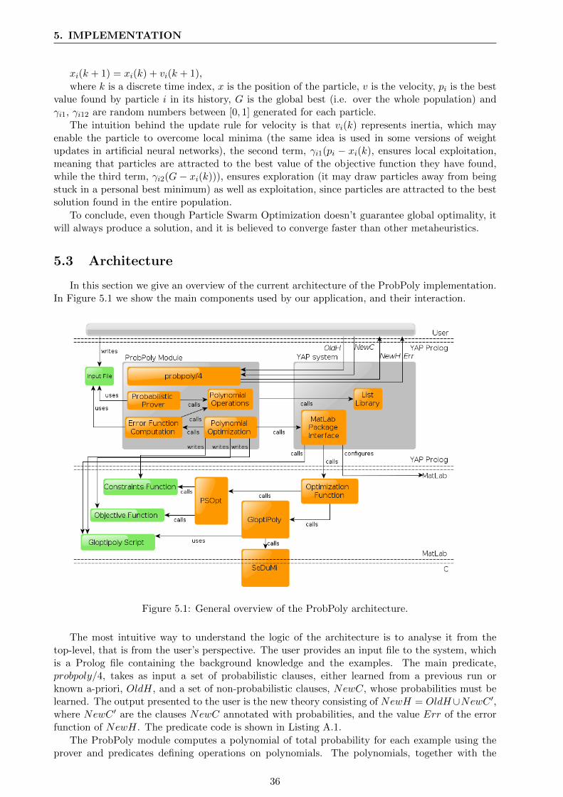
5. IMPLEMENTATION
xi(k + 1) = xi(k) + vi(k + 1),
where k is a discrete time index, x is the position of the particle, v is the velocity, pi is the bestvalue found by particle i in its history, G is the global best (i.e. over the whole population) andγi1, γi12 are random numbers between [0, 1] generated for each particle.
The intuition behind the update rule for velocity is that vi(k) represents inertia, which mayenable the particle to overcome local minima (the same idea is used in some versions of weightupdates in artificial neural networks), the second term, γi1(pi − xi(k), ensures local exploitation,meaning that particles are attracted to the best value of the objective function they have found,while the third term, γi2(G− xi(k))), ensures exploration (it may draw particles away from beingstuck in a personal best minimum) as well as exploitation, since particles are attracted to the bestsolution found in the entire population.
To conclude, even though Particle Swarm Optimization doesn’t guarantee global optimality, itwill always produce a solution, and it is believed to converge faster than other metaheuristics.
5.3 Architecture
In this section we give an overview of the current architecture of the ProbPoly implementation.In Figure 5.1 we show the main components used by our application, and their interaction.
Figure 5.1: General overview of the ProbPoly architecture.
The most intuitive way to understand the logic of the architecture is to analyse it from thetop-level, that is from the user’s perspective. The user provides an input file to the system, whichis a Prolog file containing the background knowledge and the examples. The main predicate,probpoly/4, takes as input a set of probabilistic clauses, either learned from a previous run orknown a-priori, OldH, and a set of non-probabilistic clauses, NewC, whose probabilities must belearned. The output presented to the user is the new theory consisting of NewH = OldH∪NewC ′,where NewC ′ are the clauses NewC annotated with probabilities, and the value Err of the errorfunction of NewH. The predicate code is shown in Listing A.1.
The ProbPoly module computes a polynomial of total probability for each example using theprover and predicates defining operations on polynomials. The polynomials, together with the
36

5.4 The Impact of Negation as Failure
probabilities of the examples are then used to compute the error function, which is also a polynomial.Then, this polynomial, and the constraints discussed in Section 4.3 when learning multiple clausesare sent to MatLab. For Gloptipoly, we generate a MatLab script which creates the Gloptipolyobjects needed as input for the solver:
� the polynomial object,
� the objective function, i.e. the error function
� the list of constraints
An example is given in Listing A.7.For PSOpt, we generate two MatLab function files, specifying the objective function, e.g. Listing
A.8 and the list of constraints A.9.After the generation of these files, we start and set up MatLab1 using the MatLab Package
Interface available in YAP. Then, we call a function which tries to find the global minima withGloptiPoly, and in case of failure, uses the particle swarm optimization toolbox PSOpt to searchfor global minima. We show the function in Listing A.10.
GloptiPoly uses SeDuMi, ”a software package to solve optimization problems over symmetriccones. This includes linear, quadratic, second order conic and semidefinite optimization, and anycombination of these”2, written in MatLab and C.
We believe that the current architecture is a good design choice since we can solve tasks ofsymbolical computation in Prolog, and we can use MatLab to handle numerical problems.
5.4 The Impact of Negation as Failure
Allowing negation as failure means that in the derivation of a goal, we may have to computethe total probability of a negated goal. This forces the representation of the probability of a goalas a polynomial.
If we don’t incorporate negation as failure, and consider single clause learning, we can representthe probability of a goal as a tuple:
[c, n,m], corresponding toc ∗ xn ∗ (1− x)m.This way, during the proof we simply collect [c, n,m] and when we compute the total probability
of a goal we use Theorem 2.2 for (1− x)m.A similar situation occurs in the case of multiple clause learning. We can represent the proba-
bility of a goal as a tuple:[c, p1, . . . , pk, pk+1], corresponding toc ∗ xp11 . . . xpkk ∗ (1− x1 − ...− xk)pk+1 .Again, during the proof we collect only [c, p1, . . . , pk, pk+1] and when evaluating the total prob-
ability of a goal we use Theorem 2.3 to compute (1− x1 − ...− xk)pk+1 .
1The most important operation is to add the MatLab folder and its subfolders to the MatLab path.2Quote from the FAQ of SeDuMi (http://sedumi.ie.lehigh.edu/ – accessed 08.09.2011)
37

Part II
Towards Learning ProbabilisticRequirements
38

Chapter 6
Related Work in LearningRequirements
It is essential to have an overview of the state-of-the-art systems used in modelling and learningrequirements, in order to be able to develop a solution for models which incorporate probabilities.In Section 6.1 we briefly present a system which uses ILP and a model checker in a learner-teacherparadigm. A similar approach, which uses artificial neural networks adapted for linear temporallogic instead of ILP, is described in Section 6.2. Automated verification and learning assumptionsfor models is the topic of Section 6.3, and the studied system uses the L* algorithm as a learner,with counterexamples provided by a model checker. Finally, we review two robust frameworkswhich have been developed for a long time, the KAOS and i* approaches to modelling and learningrequirements in Sections 6.4 and 6.5. KAOS and i* don’t take into account uncertainty in theform of probabilities, so it is important to study them to research the possibility of integratingprobabilistic reasoning in their models and methods.
6.1 Learning Requirements using ILP and Model Checking
In [Alrajeh et al., 2006], a novel method of learning requirements from scenarios is presented.The problem is to automate the process of requirement elicitation, which is a crucial part of therequirements engineering process. The raw input represents a narrative which partially describesthe requirements of the system-to-be. This is processed into a formal representation, which relies onLinear Temporal Logic (LTL) to define requirements specification Spec as a LTL theory consistingof axioms(two initial state axioms, two persistence axioms and two change axioms) and eventprecondition axioms. A scenario is a specific type of an LTL formula. Scenarios can be desirable orundesirable. The solution to the problem become finding a set of event precondition axioms Presuch that all desirable scenarios are true and all undesirable scenarios are false:
� Spec ∪ Pre |=M ¬Pu, for each undesirable scenario Pu ∈ Und.
� Spec ∪ Pre 2M ¬Pd, for each desirable scenario Pd ∈ Des.
Und and Des are the sets of undesirable and desirable scenarios. M is an LTL model of the form〈T, V 〉, where T is a Label Transitioning System (LTS), and V is a valuation function.
In order to accomplish this, specifications and scenarios are translated using an Event Calculus(EC) framework into normal logic programs. Two transformation methods are presented: one forthe specification, and one for the specification together with the sets of desirable and undesirablescenarios. The result is a background knowledge B (which includes four EC core axioms), and aset of positive and negative examples E. This is the standard input to an ILP algorithm, and inthe system described XHAIL (Extended Hybrid Abductive and Inductive Learning) is applied inorder to learn hypotheses H. These are shown, for a case study of a mine pump control system, tocorrespond to the correct event precondition axioms.
The work in [Alrajeh et al., 2009b] extends the framework presented in the previous subsection(based on [Alrajeh et al., 2006]). The main difference represents the fact that the latter is able to
39

6. RELATED WORK IN LEARNING REQUIREMENTS
handle trigger axioms, as well as precondition axioms in the LTL formalism of defining a specifica-tion, and thus the newer system is able to learn trigger conditions. This is not a trivial extension ofthe previous system, and in what follows we will briefly present the changes this extension implies.First of all, since we need a new predicate, called ”triggered”, we must define additional EC coreaxioms which describe properties of triggered events, e.g. if an event is triggered at one point intime, then all other events must be impossible at that point1. The specification LTL theory isenriched with trigger-condition axioms, similar in structure with the pre-condition axioms, denotedin [Alrajeh et al., 2006] as event precondition axioms. The way to define positive and negativescenarios is also slightly different.
Since the solution will consist of trigger-condition axioms, in addition to pre-condition axioms,we will have to find the sets of axioms Pre and Trig such that Spec ∪ Pre ∪ Trig |=M ¬Pu andSpec∪Pre∪Trig 2M ¬Pd. The translation into an EC normal logic program is naturally extendedto Trig axioms. Some theoretical results are also presented (Theorems 3.1 and 3.2), one (3.2)suggesting that we may perform the inverse translation of H into LTL formulas corresponding toaxioms (due to the inverse of the translation function τ−1). Also, the examples are fewer than in[Alrajeh et al., 2006], and more hypotheses are generated, both correct with respect to the learningtask. It is up to the engineer to choose one more appropriate, or more easily to interpret.
The system proposed in [Alrajeh et al., 2009a] represents a further improvement of the previouswork in [Alrajeh et al., 2006] and [Alrajeh et al., 2009b]. The essential novelty is the fact thatcounterexamples are generated by using the LTSA model checker (in a semi-automated process).First of all, the input changes: we now have only a partial specification which needs to be refined,and a set of goals such that the learned specification will be able to satisfy all the given goals.This is only a semi-automated procedure because, based on the trace given by the model checker,we still have to manually develop a negative scenario. In the same manner, positive scenarios areelaborated, in the case that the model checker doesn’t return a goal violation. These, as usual, willbe translated into a normal logic program, which is fed to the ILP learner. The result of the ILPmodule is a set of hypotheses which are finally translated back into requirements from which theengineer selects the adequate ones (although all are formally correct from the ILP perspective) tobe added to the specification.
6.2 Connectionist Systems for Learning Requirements
In [Borges et al., 2010b], the authors propose a new framework for knowledge representation,reasoning and learning, which is applied to the task of learning requirements from scenarios, inspiredfrom [Alrajeh et al., 2009b]. The premises and goals are essentially the same, and the case studyand main example of the article is the mine pump system, but the ILP part is replaced witha connectionist system. In this connectionist system, illustrated in Figure 6.1 (reproduced fromfigure 1 in [Borges et al., 2010b]), the model description is translated into a neural network, whichis trained using examples from the observed system and from the specified properties. The nextstep involves extracting knowledge from the trained network in the form of state diagrams, whichcan be translated into logic programs.
1EC core axiom (6) in [Alrajeh et al., 2009b].
40

6.2 Connectionist Systems for Learning Requirements
Figure 6.1: Learning framework for the connectionist system.
The representation of knowledge is based on Linear Temporal Logic (without event calcu-lus, unlike [Alrajeh et al., 2009b]). The inputs of the network are states or inputs of the system,and the main role of the network is to learn given states s1, s2, ..., sn and inputs i1, i2, ..., im,the temporal logic next state operator e, i.e. es1, es2, ..., esn. The input nodes of the net-work consist of a corresponding node for each state and input, respectively, and the outputnodes represent es1, es2, ..., esn. If the model description consists of rules of the type: esi ←s1, s2, ..., sk, i1, i2, ..., il, where the states or inputs may be negated, then for each such rule a hiddenneuron is added to the network, with inputs connections from s1, s2, ..., sk, i1, i2, ..., il and outputconnection to esi. The idea resembles the core method translation algorithm for networks sim-ulating propositional logic programs (the algorithm can be found in the proof of Theorem 3.2 in[Hitzler et al., 2004]).
The training using input/output patterns is simple, however in the case where learning isaccomplished by presenting properties to the system, the authors propose a method of defin-ing the output of the network based on a list of active properties, which is in turn determinedby the values of the current states and inputs. The example given for this step however isnot completely clear. After training, knowledge is extracted in a greedy manner: each tuple〈s1, s2, ..., sn; i1, i2, ..., im; es1, es2, ..., esn〉 appearing in the network increases the count of the sametransition, and transitions are filtered according to their counts. Each transition can be then rewrit-ten into a set of rules to obtain a logic program.
The experiments carried out on the mine pump example suggest that the framework is successfulin learning in the absence of background knowledge, and the authors argue that their method is aviable alternative to the one proposed in [Alrajeh et al., 2009b] because the connectionist systemis able to correct eventual errors in the initial description.
An extension of this system, described in [Borges et al., 2010a] incorporates the NuSMV modelchecker, probably inspired by the framework in [Alrajeh et al., 2009a], An important idea is thatthe initial knowledge may or may not be incorporated in the adaptation process. In the casewhen initial knowledge is given, it is represented as a NuSMV model, which is translated intoa logic program, and finally, the temporal logic program is used to create a neural network, viathe Sequential Connectionist Temporal Logic tool. Otherwise, the system will adapt based on theobserved system behaviour, only through examples fed into the network. After the network istrained, its output representing a symbolic model is verified against the model checker. If there areany properties not satisfied by the model, at least one counterexample is generated, and this canbe used in a similar way to examples for the neural network to adapt. The framework is shown inFigure 6.2, which is reproduced from figure 1 in [Borges et al., 2010a].
41

6. RELATED WORK IN LEARNING REQUIREMENTS
Figure 6.2: Learning framework for the connectionist system incorporating the NuSMV modelchecker.
The process of adaptation to counterexamples is very similar to learning from properties: basedon sequences of states and inputs, the system determines which inputs would generate propertyviolations at the next state, and doesn’t allow these inputs to activate in the network. Knowledgeextraction is performed in a similar way as in the previous framework. The main example remainsthe mine pump system, and it is reported that even without initial knowledge, the connectionistsystem can be successfully trained and adapted to learn the correct model.
6.3 Automated Verification of Systems using L*
6.3.1 The L* Algorithm
In [Angluin, 1987], the L∗ algorithm for learning regular sets is proposed. The algorithm is theLearner in a Teacher-Learner framework, because it depends on information given by a (minimallyadequate) teacher regarding membership queries and conjectures. The teacher must be able toanswer whether a string is a member of the set or not (i.e. answer to a membership query), andmust be able to compare the learned set S (i.e. make a conjecture) with the unknown language,and its answer must be yes in the case they are equal, or no otherwise. In the latter case, theteacher must also give a counterexample, that is a string which is in S but not in the unknownlanguage.
L∗ relies on an observation table (S,E, T ), consisting of a set of candidate strings S, a set ofdistinguishing experiments E and a mapping T : (S ∪ S ·A) ·E → {0, 1}, where A is the alphabetover which the strings are defined. By row(s) we will denote T (s · e). Based on an observationtable (S,E, T ) we define a deterministic finite-state acceptor M(S,E, T ):
, where Q is the state set, q0 is the initial state, F are the accepting states, and δ is the transitionfunction.
Two properties of observation tables are relevant: closure and consistency. An observation tableis closed if for each t in S ·A there exists a state s in S such that row(s) = row(t). An observationtable is consistent if for states s1 and s2 in S, and row(s1) = row(s2), then for all a in A we haverow(s1 · a) = row(s2 · a).
We now present the L∗ algorithm in Figure 6.3 (Figure 1 in [Angluin, 1987]). After initialization,in which the candidate states S and the distinguishing strings E are both the null string λ, themain loop of the algorithm has three important parts:
42

6.3 Automated Verification of Systems using L*
� assure that the observation table (S,E, T ) is closed consistent, which is performed usingmembership queries.
� define, as described above, the deterministic finite-state acceptor M = M(S,E, T ).
� make the conjecture M , and if the teacher replies with no, update the observation tableaccording to the counterexample provided, otherwise halt and return M .
Figure 6.3: The L∗ algorithm.
An important practical issue with the algorithm is the verification of the conjecture. Thisquery might prove infeasible in general languages. To overcome this problem, the author proposesa different method to perform the conjecture query: assuming there is a probability P on the setof all strings of alphabet A, then the query will consist of sampling a number of strings from Aaccording to P , and if any of the sampled strings are in the unknown language U and not acceptedby M(S,E, T ) or vice versa, then the answer is no, and the counterexample is the correspondingstring.
We will briefly cover an improvement of L∗ for the case in which we are not allowed to ”reset”the finite-state-machine, i.e. we are not allowed to execute sequences from the initial state, butonly from the current state. The algorithm is described in [Rivest and Schapire, 1989] and relieson two important ideas. The first one is that the finite state automaton has a finite number ofequivalence classes, defined by the equivalence relation t1 ≡ t2, which means sequences t1 and t2have the same value at every state.
The second idea is to define a homing sequence as ”an action sequence h for which the statereached by executing h is uniquely determined by the output produced”2. The output producedmeans the vector of values with the same length as h, where the i-th component means the valueafter executing the prefix of length i of h. The algorithm will only execute homing sequences, andbased on their output, it will create a separate L∗ learner, or if one already exists, it will executethe next query. By using a different learner for each output, we essentially simulate L∗ for multiplestarting states (corresponding to the ones defined by the output of executing the homing sequence).
In Figure 6.43 we reproduce the algorithm for finding a homing sequence given a finite stateautomaton, and in Figure 6.54 we show the algorithm for inferring the finite state automaton given
2Definition 2 in [Rivest and Schapire, 1989].3Figure 3 in [Rivest and Schapire, 1989].4Figure 5 in [Rivest and Schapire, 1989].
43

6. RELATED WORK IN LEARNING REQUIREMENTS
access to it, and a homing sequence. The authors also provide a slightly more complicated variantof the algorithm, in which the homing sequence is constructed simultaneously with the inferenceprocedure. They also propose algorithms for stochastic inference (infer U with probability 1− δ),algorithms which use explicitly the equivalence classes of the finite state automaton and similarinference algorithms for permutation automata.
Figure 6.4: Algorithm for finding a homing sequence.
Figure 6.5: Algorithm for inferring a finite state automaton using a homing sequence.
6.3.2 The Original Framework
In this subsection we will discuss the framework in [Pasareanu et al., 2008] which aims at veri-fying systems in an automatic way, using L∗ as a learner and the LTSA model checker as part of theteacher. The fundamental principle is to verify that all the system components satisfy some prop-erties under certain assumptions, and use parallel composition to prove that the safety propertyholds for the whole system.
Let us introduce a few notions. A labelled transition system (LTS) is a four-tuple M =〈Q,αM, δ, q0〉, where Q is the set of states, αM is the alphabet of the LTS, δ is the transitionrelation consisting of a source state, an action, and a destination state, and q0 is the initial state.The parallel composition of two labelled transition systems M1 ‖M2 is also an LTS. A safety LTSis a LTS which doesn’t contain an error state. A safety property is ”a safety LTS P whose languageL(P ) defines the set of acceptable behaviors over αP”. Based on a property, we define an errorLTS, Perr, which extends P so that all the transitions which are not in the LTS lead to an errorstate. The purpose of this is to detect violations of the safety property. Finally, an assume guaran-tee formula is a triple 〈A〉M〈P 〉 in which M is a component (in this case an LTS), P is a property(as defined above), and A is an assumption about the environment of M (typically a conjecturelearned by L∗).
An important theoretical result is Thoerem 1 of [Pasareanu et al., 2008], which states that:〈A〉M〈P 〉 is true if and only if the error state is unreachable from A ‖ M ‖ Perr. The assumeguarantee formulas are used to make rules which guarantee the satisfaction of a property by thesystem. In Figures 4 and 5 (reproduced from [Pasareanu et al., 2008]) we have two such rules.The first rule, ASYM, states that if the property A should hold for a component, and if the othercomponent satisfies property P under the assumption of A, then the system satisfies P . This rulecan be generalized such that it incorporates circularity between n components (it is described asrule CIRC-N in [Pasareanu et al., 2008]). The second rule states that if each component satisfies
44

6.3 Automated Verification of Systems using L*
P under its own assumption, and if the languages of the complements (coAi) of the assumptionsare a subset of the language of P , then the system satisfies P . The complement of an LTS M isan LTS which accepts the complement of M ’s language.
Figure 6.6: Rule ASYM.
Figure 6.7: Rule SYM.
To complete the presentation, we show an algorithm for rule ASYM in Figure 6.8 (Figure 4from [Pasareanu et al., 2008]). The top box of the Teacher represents the membership query toL∗, and the three bottom boxes of the Teacher represent the conjecture query. In the latter case,the oracles illustrate methods to check the premises of ASYM. Notice that if the second premiseis false, the counterexample is not immediately returned to L∗, instead further counterexampleanalysis is performed, and if the counterexample is valid, than a real error trace is returned to theuser, otherwise the Teacher returns to L∗ the correct conjecture.
Figure 6.8: Alogrithm for rule ASYM.
The reason we are interested in L∗ and more importantly the application briefly described isthat extracting requirements is similar to system verification in the sense that the property to besatisfied represents the fact that the learned requirements must not violate system constraints.Moreover, both techniques have made use of a model checker, with the same goal of generatingcounterexamples, however L∗ has not been tried as a method to learn requirements, and thisprovides a novel direction of research.
45

6. RELATED WORK IN LEARNING REQUIREMENTS
6.3.3 Verification in a Probabilistic Context
The probabilistic extension of assume-guarantee reasoning is introduced in [Feng et al., 2011].The same authors developed PRISM - a probabilistic model checker which is used to verify proba-bilistic properties. We will describe probabilistic model checking, its properties and models in thenext chapter, however we exemplify a few properties, since they are used to parametrize assump-tions. In a probabilistic context we can verify more expressive properties such as5:
� security properties like: ”the probability of an airbag failing to deploy within 0.02 seconds isat most 0.0001”,
� timeliness properties like: ”expected time for a successful transmission of a data packet”
Properties of the type G: �¬fail become 〈�¬fail〉≥0.98. Adversaries ( also known as strategies,schedulers, policies) are possible ways to incorporate non-determinism in probabilistic models, andare generally defined as functions which given a state, produce an action.
Let us assume a model like an LTS, with the difference that once an action is chosen, in a state,the next state is determined probabilistically. A model M satisfies property 〈G〉≥pG (M |= 〈G〉≥pG)if PrσM (G) ≥ pG for all adversaries σ. The assume guarantee triple becomes 〈A〉≥pAMi〈G〉≥pG ,with Mi a model, and 〈A〉≥pA , 〈G〉≥pG are safety properties whose extension would lead to badtraces.
The key idea of the learning process is to reduce the probabilistic checking of properties to theproblem of learning a non-probabilistic assumption, by exploiting properties of the adapted ASYMrule and using a variant of the L* algorithm.
We leave out the technical details because we will define probabilistic models in the next chapter,and, for our purposes, the important aspect of this system is the use of a probabilistic model checkerin conjunction with a learner to generate properties of probabilistic models.
6.4 The KAOS framework and related methods
6.4.1 Introduction and Inference of Requirements Specifications from Scenarios
KAOS is a methodology which enables the modelling of requirements and automatic generationof requirements based on goals or scenarios6. This brief introduction to KAOS and the rest of thesubsection is based on [van Lamsweerde and Willemet, 1998], which shortly describes the KAOSsystem, starting from its ontology:
� Object - can be an entity, relationship or event, characterized by attributes and invariantassertions.
� Operation - input/output relation between objects, characterized by pre-, post- and trigger-conditions. The pre- and post-conditions are classified into domain and required condition,the former being general constraints, while the latter capture additional conditions.
� Agent - a type of object which is allowed to perform certain operations on other objects.
� Goal - an objective the system should meet. Goals are usually refined in AND/OR graphs (agoal is satisfied if all the sub-goals are satisfied in an AND-refinement, or it is satisfied if atleast one sub-goal is satisfied in an OR-refinement). Goals involve certain Objects, and mayconflict with each other.
� Requisite, requirement, assumption. A requisite is a goal which can be controlled by an indi-vidual agent. Refinements must transform the initial goal into a set of requisites. Require-ments are requisites assigned to software agents, while assumptions are requisites assigned toenvironmental agents.
5Examples are reproduced from [Feng et al., 2011].6For an extensive list of publications see: http://www.info.ucl.ac.be/~avl/ReqEng.html (accessed 08.09.2011).
46

6.4 The KAOS framework and related methods
In what follows, we will give examples of some of these concepts. In Figure 6.9 (reproduced fromsection 2.1.2) we can see a goal specification. We notice object instantiation, the objects involvedin the goal definition, the informal definition, which is implemented in the system in the context ofa semantic net, the goals which refine the initial goal (it is the case of an AND-refinement), and theformal definition, which expresses the same idea as the informal one, but in the syntax of temporallogic.
Figure 6.9: Goal specification.
For an example of an operation we refer to Figure 6.107. Notice the input instances of objects”Card” and ”Amount-$”, and the output object ”Cash Delivered” (of type event). It was estab-lished that operations are performed by agents, so the definition must specify it, in this case, aninstance of the ”ATM” object. Finally, the domain pre- and post-conditions are shown. However,taking into account the goal specification, we also need to add required pre-post conditions. Apossible pre-condition would be to check if the password is entered correctly.
Figure 6.10: Definition of an Operation.
In what follows, we will briefly present the KAOS specification elaboration method starting fromhigh-level goals, and some aspects of the goal-inference procedure from scenarios. The method ofspecification elaboration consists of several steps:
1. Goal elaboration - this steps involves goal refinement until requisites, as previously defined,are reached.
2. Object and operation capture - identifies relevant objects and operations to the goal formula-tions.
3. Operationalization - generates additional conditions for operations in order to satisfy therequisites obtained after goal elaboration.
4. Responsibility assignment - this final step is concerning the management of requisites, theirdistribution among agents, solving conflicts caused by the different goals of the stakeholdersetc.
This framework has been enriched to allow scenarios as input, besides or instead of goals, andsuch a change gave rise to the problem of inferring goals from scenarios. Scenarios are given in theform of event trace diagrams, and can be positive or negative. Initially, scenarios are pre-processedin order to aggregate events, eliminate irrelevant events to the software agents, or to some scope ofinterest. The goals inferred may be of two types:
7Reproduced from section 2.1.2 of [van Lamsweerde and Willemet, 1998].
47

6. RELATED WORK IN LEARNING REQUIREMENTS
� Achieve/Cease - formally P ⇒ ♦Q (where ♦ means at some point in the future, and ⇒expresses a usual implication that holds irrespective of the time, formally P ⇒ Q iff �(P →Q), and � means always in the future).
� Maintain/Avoid - formally P ⇒ Q W R, where W means always in the future unless
The goals inferred should cover all positive scenarios and exclude all the negative ones, similarlyto the ILP learning setting. The most important steps of the inference method (presented in section4.1 and detailed in sections 4.2 - 4.7 of [van Lamsweerde and Willemet, 1998]) are the collection ofprogress facts (formally, Pre−State→ ePost− state, where Pre−State and Post− state are thestates before and after the event), and invariance facts (formally, R ∧ ST → (R W N), where R isa condition that remains true from state transition ST until another condition N becomes true).Subsequently, progress facts and invariance facts are generalized. We will focus on generalizationover time and over instances. In generalization over time, implications (→) are generalized over allstates into⇒, and for progress facts, the next state operator ( e) is generalized into some time in thefuture (♦). In generalization over instances, the ground assertions are generalized in a weak mannerby introducing existentially quantified variables or in a strong manner by introducing universallyquantified variables.
To conclude, although there are more steps in the scenario elaboration process, we believe thatthe inference process is a crucial one. The final output of the system depends entirely on the goalsinferred, and consists of specifications formally represented by temporal logic formulas involvingagents, objects and operations.
6.4.2 Conflicts and Obstacles in Goal-Driven Requirements Engineering
This subsection briefly highlights the key ideas regarding how the KAOS system handlesgoal conflicts and obstacles, based on the work published in [van Lamsweerde et al., 1998] and[van Lamsweerde and Letier, 2000]. The detection and resolution of conflicts is integrated in thescenario elaboration framework in relation with goal elaboration. After conflicts are detected basedon current goals, several solutions generate, modify or delete goals. There are also solutions inwhich conflicts are resolved by assigning the responsibilities to different agents, so there is also aconnection between responsibility assignment and conflict resolution.
Inconsistencies can be of different types and relate to different aspects of requirements specifica-tions. Inspired by [van Lamsweerde et al., 1998], we will mention here only the notions of conflict,divergence and obstruction:
� Conflict - occurs between assertions A1, ..., An in a domain Dom if:
1) (Dom,∧1≤i≤nAi) ` false and
2) ∀i, 1 ≤ i ≤ n, (Dom,∧j 6=iAj) 0 false.The first condition states that there must be an inconsistency between the assertions inthe domain, and the second condition enforces minimality, that is if we remove any of theassertions, there remaining assertions in the domain do not cause a conflict.
� Divergence - occurs between assertions A1, ..., An in a domain Dom if there exists a boundarycondition B, such that:
1) (Dom,B,∧1≤i≤nAi) ` false,2) ∀i, 1 ≤ i ≤ n, (Dom,B,∧j 6=iAj) 0 false and
3) ∃ scenario S and a time position i such that (S, i) � B.
The boundary condition B is a particular circumstance generated by scenario which givesrise to a conflict when taken together with assertions A1, ..., An.
� Obstruction - represents the limiting case of a divergence when n = 1, i.e. we have only onegoal assertion. Then, the boundary condition B is called an obstacle to the goal assertion A.
48
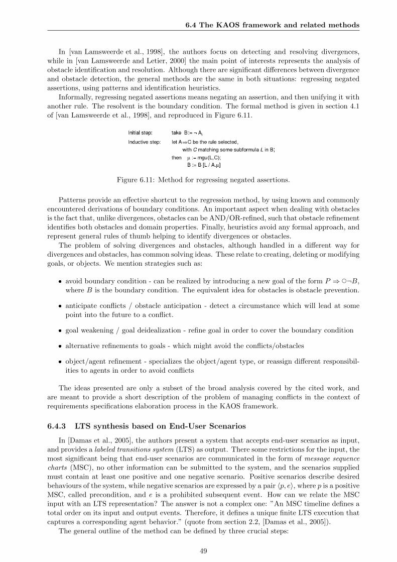
6.4 The KAOS framework and related methods
In [van Lamsweerde et al., 1998], the authors focus on detecting and resolving divergences,while in [van Lamsweerde and Letier, 2000] the main point of interests represents the analysis ofobstacle identification and resolution. Although there are significant differences between divergenceand obstacle detection, the general methods are the same in both situations: regressing negatedassertions, using patterns and identification heuristics.
Informally, regressing negated assertions means negating an assertion, and then unifying it withanother rule. The resolvent is the boundary condition. The formal method is given in section 4.1of [van Lamsweerde et al., 1998], and reproduced in Figure 6.11.
Figure 6.11: Method for regressing negated assertions.
Patterns provide an effective shortcut to the regression method, by using known and commonlyencountered derivations of boundary conditions. An important aspect when dealing with obstaclesis the fact that, unlike divergences, obstacles can be AND/OR-refined, such that obstacle refinementidentifies both obstacles and domain properties. Finally, heuristics avoid any formal approach, andrepresent general rules of thumb helping to identify divergences or obstacles.
The problem of solving divergences and obstacles, although handled in a different way fordivergences and obstacles, has common solving ideas. These relate to creating, deleting or modifyinggoals, or objects. We mention strategies such as:
� avoid boundary condition - can be realized by introducing a new goal of the form P ⇒ e¬B,where B is the boundary condition. The equivalent idea for obstacles is obstacle prevention.
� anticipate conflicts / obstacle anticipation - detect a circumstance which will lead at somepoint into the future to a conflict.
� goal weakening / goal deidealization - refine goal in order to cover the boundary condition
� alternative refinements to goals - which might avoid the conflicts/obstacles
� object/agent refinement - specializes the object/agent type, or reassign different responsibil-ities to agents in order to avoid conflicts
The ideas presented are only a subset of the broad analysis covered by the cited work, andare meant to provide a short description of the problem of managing conflicts in the context ofrequirements specifications elaboration process in the KAOS framework.
6.4.3 LTS synthesis based on End-User Scenarios
In [Damas et al., 2005], the authors present a system that accepts end-user scenarios as input,and provides a labeled transitions system (LTS) as output. There some restrictions for the input, themost significant being that end-user scenarios are communicated in the form of message sequencecharts (MSC), no other information can be submitted to the system, and the scenarios suppliedmust contain at least one positive and one negative scenario. Positive scenarios describe desiredbehaviours of the system, while negative scenarios are expressed by a pair 〈p, e〉, where p is a positiveMSC, called precondition, and e is a prohibited subsequent event. How can we relate the MSCinput with an LTS representation? The answer is not a complex one: ”An MSC timeline defines atotal order on its input and output events. Therefore, it defines a unique finite LTS execution thatcaptures a corresponding agent behavior.” (quote from section 2.2, [Damas et al., 2005]).
The general outline of the method can be defined by three crucial steps:
49

6. RELATED WORK IN LEARNING REQUIREMENTS
1. Submitting an initial set of positive and negative scenarios.
2. Generating scenario questions and synthesizing agent LTS.
3. Generating state invariants to document the generated state machines.
The first two steps are detailed in the algorithm in Figure 6.12 (reproduced from figure 11 from[Damas et al., 2005]). We will refer to the automaton A in the algorithm as an LTS, keeping inmind the difference that in an LTS all states are accepting states, while in an automaton only asubset of the possible states contains accepting states. The LTS is initialized such that it coversall positive scenarios, by constructing a prefix tree acceptor PTA(S+), that is the largest DFA(deterministic finite-state acceptor) that accepts the strings from S+. This DFA will be generalizedby merging a pair of states chosen according to a lexicographical order, and a potential update(Anew) of the LTS is created by merging 8 the two states. First of all, the potential update LTShas to be compatible with the negative scenarios (S−), i.e. every string in S− has to be rejectedby Anew.
If Anew is compatible with S−, the system will follow step 2, i.e. it will interact with the userthrough a series of questions, which essentially try to determine whether extensions of sequencesaccepted by A which are accepted by Anew are correct positive scenarios. As we can see in thefigure below, in the if CheckWithEndUser branches, if the answer is affirmative, then the extendedsequence is added as a new positive scenario, otherwise as a new negative scenario, and in thislatter situation, the potential update DFA Anew is no longer an acceptable update.
Figure 6.12: Algorithm for LTS generation based on end-user scenarios.
Step three involves generating state invariants from fluent definitions. We will not describe theprocess here, but we mention it is an important step to help visualize the final LTS. To conclude,two potential directions of investigation shall be hinted. Is it possible to learn without initialnegative scenarios from the end-user? Even in the current framework, negative scenarios can begenerated by a negative answer to an end-user question, but perhaps a possibility would be to usethe model-checking to generate negative scenarios. Another improvement might concern the choiceof merging states, depending on the answer to the question: is there an ”intelligent” way to choosethe states to be merged?
8Merging is not a trivial process: the resulting DFA, called a quotient automaton, might not be deterministic, andfurther merging of states would be necessary.
50

6.5 The I* Approach
6.5 The I* Approach
The i* methodology proposes an alternative perspective on modelling requirements. Insteadof focusing on scenarios or goals, the fundamental unit of its philosophy is the intentional agent,equipped with individual goals, beliefs, abilities and other properties, which are not always knownor controllable. Agents depend on each other to reach their goals, share or trade resources andso on. Modelling a system as a complex interaction between agents is one of the reason i* is alsoreferred to as social modelling.
Intentionality is either explicit, via goals which are decomposed into subgoals, or into means-ends alternatives, an idea which is similar to the AND/OR graph decomposition in KAOS. Inten-tionality expressed by agents is called implicit, because we might not have access to their internalgoals, and is manifested thorough links between agents, which are called dependencies.
Dependencies are classified into:
� goal dependencies - are typically assertions, with no preference for the way of ensuring them;
� task dependencies - indicate precise activities which are expected from an agent
� resource dependencies - model the dynamics of entities which can be shared or transmittedbetween agents
� soft-goal dependencies - are similar to goal dependencies, with the mention that they claim aquality of the interaction, rather than a precise, binary assertion. This type of dependenciesis used to model non-functional requirements.
Unfortunately, i* affords only a qualitative analysis of requirements, so the task of integratingquantitative measures such as probabilities remains a challenge which we hope to address in futurework.
51

Chapter 7
Modelling and Verification.Probabilistic Model Checking.
In the previous part we have presented out contribution to PILP using SLPs, the ProbPolyframework. In this chapter we aim to show how we might adapt a methodology for learningrequirements using model checking and ILP to the probabilistic context, using probabilistic modelchecking and PILP, and more specifically, ProbPoly. To our knowledge, this is an unexploredarea of research, and the most relevant system which learns probabilistic assumptions is the onereviewed in Section 6.3, but it uses probabilistic model checking in conjunction with an modifiedversion of L*. We demonstrate our novel approach of combining probabilistic model checking andlogic learning as a teacher-learner method on a small example.
After the previous reviews of a range of relevant systems which focus on modelling and some alsoon learning requirements in Chapter 6, we introduce the main challenge of learning requirements,and begin to reason on how we may overcome it by using ProbPoly. Section 7.1 establishes thepremises of our approach, so that we are able to offer a simple, yet representative example inSection 7.2. Finally, in Section 7.3 we discuss the main questions which motivate directions offuture research.
7.1 Probabilistic Model Checking. PRISM.
Probabilistic model checking is a framework for the verification and analysis of probabilisticfinite-state models, which are checked against probabilistic properties, e.g. formulas in probabilisticextensions of temporal logic. Unlike traditional model checking, the probabilistic extension cananalyse properties of quantitative nature, e.g. ”the system will reach a fail state in at most k timeunits with a probability less than 0.02”. In this example, the probability can be computed based onthe probabilities of the model, and the k time units is expressed in terms of costs (or equivalentlyrewards).
The result of checking a property is a truth value, expressing whether the property is satisfiedor not. In the case that the property holds, additional output may consist of a lower and/or anupper bound on the probability of the respective property. In the case that the property isn’tsatisfied, a counterexample should be given, that is a set of traces through the model which violatethe property. The definition and computation of counterexamples in probabilistic model checkingis an active research topic among software engineers. We will give an intuitive definition of whatwe believe is the best counterexample in Section 7.2.
Probabilistic model checking must have efficient data structures (e.g. BDDs) and numericalalgorithms for computation of the different quantities, in order to allow large-scale models. Togain a better understanding of probabilistic model checking, let us look at what type of models arecommonly used in the field.
The fundamental problem of designing a system that learns requirements is the representationof the domain and of the software system. We believe that the LTS, as presented in Section 6.3,is a state-of-the-art representation for systems which don’t incorporate probability, and in the
52

7.1 Probabilistic Model Checking. PRISM.
probabilistic context perhaps the most popular models are:
� Discrete Time Markov Chains (DTMCs),
� Continuous Time Markov Chains (CTMCs), also known as Continuous Time Markov Pro-cesses,
� Markov Decision Processes (MDPs), which are almost equivalent to Probabilistic Automata(PA). We will use the latter in our terminology.
The simplest model is a DTMC:
Definition 7.1 ((Discrete Time) Markov Chain). A Discrete Time Markov Chain, as defined in[Manning and Schutze, 1999], is a sequence of random variables X = (X1, . . . , XT ) taking valuesin some finite set S = {s1, . . . , sN}, the state space and satisfies the Markov Properties:
� Limited Horizon:P (Xt+1 = sk|X1, . . . , Xt) = P (Xt+1 = sk|Xt)
� Time invariant (stationary):P (Xt+1 = sk|Xt) = P (X2 = sk|X1), where ∀t, t+ 1 ∈ 1, . . . , T and ∀k ∈ 1, . . . , N
The time invariance condition is sometimes omitted, or mentioned as a property of a specialcase of Markov Chains (time-homogeneous or stationary), and is usually defined in a more intuitiveway:
P (Xt+1 = sk|Xt = sl) = P (Xt = sk|Xt−1 = sl)
A DTMC is described by a stochastic transition matrix A with entries:
aij = P (Xt+1 = sj |Xt = si), with
aij ≥ 0, ∀i, j ∈ 1, . . . , N andN∑j=1
aij = 1, ∀i ∈ 1, . . . , N .
Usually, Markov chains are also characterized by the probabilities on the initial states:
πi = P (X1 = si), withN∑i=1
πi = 1.
However, we can always add an extra ”start” state, such that P (X1 = start) = 1, and thereforethe probabilities πi are pushed into the transition matrix A. We will indeed choose to characterizea DTMC only by matrix A.
Let us exemplify a DTMC which illustrates a fair six-sided die. This example is considered as acase study in the probabilistic model checker PRISM (which we will discuss a little later) and wasoriginally presented in [Knuth and Yao, 1976].
Example 7.1 (Fair Six-Sided Die DTMC). The transition matrix for this DTMC is sparse, so wewill represent it as such1:
1A list of 〈i, j, p〉 tuples such that i, j ∈ 1, . . . , N , aij = p, and for all omitted pairs k, l, with k, l ∈ 1, . . . , N ,akl = 0.
53

7. MODELLING AND VERIFICATION. PROBABILISTIC MODEL CHECKING.
From To Transition Probability
0 1 0.5
0 2 0.5
1 3 0.5
1 4 0.5
2 5 0.5
2 6 0.5
3 1 0.5
3 7 0.5
4 8 0.5
4 9 0.5
5 10 0.5
5 11 0.5
6 2 0.5
6 12 0.5
7 7 1
8 8 1
9 9 1
10 10 1
11 11 1
12 12 1
Although this is an acceptable mathematical and computational representation, we understandDTMCs much easier if they are expressed graphically in Figure 7.1:
Figure 7.1: DTMC for a Fair Six-Sided Die. The dashed lines and die images are included to relatethe model to its semantics; they are not part of the DTMC.
CTMCs are essentially DTMCs with continuous indexes instead of discrete ones. We don’ttreat them formally since we haven’t done any experiments involving CTMCs yet.
Probabilistic Automata (PA) combine DTMCs and LTSs in an expressive way: from every statewe must choose an action, in a non-deterministic fashion, similar to the LTS case, however, we aren’tguaranteed to reach a single destination state. Instead, we have a function trans : N ×M ×N →[0, 1], where N is the number of states, and M is the set of actions, such that:
N∑j=1
trans(i, a, j) = 1, ∀i ∈ 1, . . . , N, a ∈M .
In Figure 7.2 we show two PA from [Kwiatkowska et al., 2010]. Similar to LTSs, a parallelcomposition operator can be defined on PA, but we leave out the formal details because we haven’ttested our methods on compositions of PA.
54

7.1 Probabilistic Model Checking. PRISM.
Figure 7.2: Two Probabilistic Automata from [Kwiatkowska et al., 2010].
Finally, we would like to mention that we have chosen to perform our experiments in thePRISM probabilistic model checker2 introduced in [Hinton et al., 2006]. PRISM has a very intuitivelanguage for describing models, for example let us write the two models from Figure 7.2. 3 Theresult is shown in Figure 7.3.
Figure 7.3: Prism Model of the PA in Figure 7.2.
Properties are defined in a separate file. Figure 7.4 is a snapshot of a property file loaded intoPRISM and checked against the model from Figure 7.3.
Figure 7.4: Prism Properties checked against the model from Figure 7.3.
2http://www.prismmodelchecker.org (accessed 07.09.2011).3When multiple models are defined in a single file, PRISM always considers their composition.
55

7. MODELLING AND VERIFICATION. PROBABILISTIC MODEL CHECKING.
The first property checks the maximum probability that can be reached in state t3. The formulatrue U t = 3 means that the probability must be checked at each time step until (U) we are instate t3. The second and third properties are similar to the first one: they simply check a givenprobability as a lower/upper bound for a certain state.
7.2 Learning A Simple Discrete Time Markov Chain
In this section we present the learning process of the probabilities for a six-sided die, so thattwo basic properties hold in the new model. Let us formalize our task:
Given: an initial model as a DTMC, and a list of properties which need to be satisfied,
Learn: new parameters for the DTMC such that all the properties are satisfied.
First of all notice that we only learn the parameters, and not the structure of the DTMC.The method of learning the parameters is ProbPoly, and as detailed in the first part of the thesis,ProbPoly learns a new predicate based on counterexamples, which should be generated by themodel checker4. We mentioned at the beginning of the chapter the issue of counterexamples inprobabilistic model checking. What should be a counterexample in the case of a DTMC?
Fortunately this problem has been addressed, so we adopt the definition of a counterexamplefrom [Han and Katoen, 2007]. The cited publication defines the strongest evidence as a path inthe model which has a maximum probability. The evidence may or may not be a counterexamplebased on the value of the evidence and the upper bound of a probabilistic property (of the formP<p(. . . )) that the model is checked against.
We will use the term counterexample when referring to the strongest evidence in the case thatis a counterexample, unless there is ambiguity. The key idea of computing the strongest evidenceon a DTMC is by transforming it into a weighted digraph and solving the problem of kth-shortestpath. The authors also define the smallest counterexample as the counterexample with the shortestpath, and maximum probability.
Consider the following setting:
Example 7.2 (Six-sided die). The initial model is the fair six-sided die from Example 7.1. ItsPRISM model is:
The desired properties are:
1. P < 0.15 [ true U s = 7 & d = 1 ], i.e. the probability of obtaining a die value of 1 is lessthan 0.15,
2. P < 0.02 [ true U s = 7 & d = 5 ], i.e. the probability of obtaining a die value of 5 is lessthan 0.02.
The model is not a straightforward translation of the DTMC from Example 7.1. States 7-12 ofthe DTMC from the previous section are absorbed into state 7, and we use a separate variable d
4The current version of PRISM (4.0.2) has no counterexample generation options, and it seems incompatible withthe DiPro tool http://www.inf.uni-konstanz.de/soft/dipro/ (accessed 08.09.2011)
56
7.2 Learning A Simple Discrete Time Markov Chain
to encode the value of the die in s7. This is possible because states 7-12 are all terminating states,i.e. extending a path from them is an loop of the same state with probability 1.
We may think of the die as a very simple system, and that obtaining die value 1 is an error situ-ation, and obtaining a die value of 5 is a critical error state of the system. They are checked againstthe initial model, and both properties aren’t satisfied, so we consider generating counterexamplesfor each one.
It is obvious that the counterexamples with the highest probability are:
� for the first property: c1 = [s0, s1, s3, s7, d1]. This path has a probability of 0.5 · 0.5 · 0.5 =0.125. This probability is smaller than 0.15, but take into account that the total probabilityof reaching d1 is c1 and the infinite number of paths obtained by looping n (n → ∞) timesthrough [s3, s1, s3]. Its value for the initial model is, as expected, 1/6 = 0.1(6).
� for the second property: c2 = [s0, s2, s5, s7, d5], with the same probability as c1.
The next step in our approach is to remodel the DTMC in Prolog, because at the moment weare unfamiliar with the implementation details of PRISM. The initial model is represented as abackground knowledge file in Listing A.6. Notice that each predicate has corresponds to a state,and we omit s7 and simply specify di. The counterexamples for the properties are encoded as prob-abilistic examples for ProbPoly. We can’t ensure strict inequality with the current implementationof ProbPoly, due to the fact that if we get a very small global minimum for the error function, theprobabilities tend to be equal. An important observation is also that unlike the probabilistic modelchecker, we can’t handle infinite recursion5, so we compute an incomplete probability.
The current version of ProbPoly can’t learn the probabilities of multiple predicates at the sametime, since we enforce the constraint that the probabilities of the new clauses must sum up to onewhen there are no previously learned clauses, so our approach is the following:
Algorithm 1 Learn new DTMC parameters using ProbPoly
IN: initial model file BK0, N number of statesOUT: final model BKN
for i = 1→ N doBKi ← BKi−1 \ {Pi−1 : Ci−1 | C+
i−1 = si−1}H ← Ci−1P ′i−1 : C ′i−1 ← ProbPoly(BKi, H)BKi ← BKi−1 ∪ {P ′i−1 : C ′i−1}
end for
In Algorithm 1, we are given the initial model file, and we process it according to a certainorder of the states: the probabilistic clauses for each state are removed from the background fileand added without probabilities to the theory we want to learn. Then, the new probabilistic clausesare re-added to the background file and we continue with the next state.
The output of the learning process for Example 7.2 is illustrated in Figure 7.5.
Finally, we translate the new model into PRISM and the model checker successfully verifies theinitial properties.
5The maximum recursion depth is controlled by the max proof length/1 predicate.
57

7. MODELLING AND VERIFICATION. PROBABILISTIC MODEL CHECKING.
Figure 7.5: Graphical illustration of the learned model.
7.3 Conclusions
To conclude this chapter, we present some observations about our learning procedure. Firstof all, due to the fact that, at the moment, we learn the probabilities of each state, this forcesus to use an initial model as input, and to perform learning incrementally. This is very similarto the Expectation Maximization (EM) paradigm. However, Expectation Maximization can onlyguarantee to reach a local maximum, determined by the initial parameters.
By minimizing the mean squared error function for the probabilities of each state, we get agreedy algorithm, e.g. consider the probabilities of transition from s2 in the learned model. Thisstrategy might output probabilities that simply can’t be enforced in the system. Thus, one of ourgoals is to learn a model which is as close as possible to the initial one. This is somewhat similarto the regularization idea of parametric models, e.g. weight decay in artificial neural networks. Apossible way to implement it is by modifying the error function such that each example is penalizedby adding (since our task is minimization) a value proportional to the difference between the initialvalue of the probability and the learned value.
We believe that our current strategy could be redefined in a formal EM paradigm; more impor-tantly, we are confident on the fact that minor implementation modifications will allow ProbPolyto learn multiple predicates, since it is only a matter of redefining constraints for sets of variablescorresponding to the same clause head. In this context, we could learn the parameters based ona purely structural initial model. We also speculate that using ILP in conjunction with ProbPolymight allows to combine structure learning and parameter learning for probabilistic models.
Finally, an important theoretical and practical challenge is to adapt ProbPoly to infinite pathsin the model. This is equivalent to the multivariate constrained minimization of the sum of a seriesof polynomials, an area which we haven’t researched yet.
58

Chapter 8
Future Work
Using the conclusions we have drawn from the two parts of the thesis, we can formulate a listof interesting directions to pursue in future work.
Learn probabilities for refined clauses
It is possible to perform learning in the case that clause c exists in H – let us refer to it asyj : hj – and it is refined into clause c′. This is the case in the cover loop algorithm (e.g. in FOIL[Quinlan and Cameron-Jones, 1993]) or in the ILP system HYPER, presented in [Bratko, 2000],where we consider refinements over a forest, each tree corresponding to the refinement of a clause.In this case, we could delete the clause to be refined yj : hj from the SLP and normalize the otherclauses by
y′i =yj∑
i∈1,n\{j}
yi
for hi, ∀i ∈ 1, n \ {j}. Then, the problem is the same as adding clause x′ : c′, i.e. the refinedclause, to the normalized clauses y′i : hi.
1
Use probabilistic quantities as scores that guide the ILP search
The fusion or at least interaction of structure learning and parameter learning is a promisingidea which might allow to improve the quality of the learning process. We intend to use the valueof the computed error function as a selection criterion for choosing a particular refinement, perhapscombined with traditional ILP scores.
We also plan to define measures such as precision, recall etc. for SLPs based on the quantitieswe introduced in the last subsection of Section 4.3. These measures could also be used to guide thesearch, as proven in [Raedt and Thon, 2010].
Extend ProbPoly to learning multiple predicates simultaneously
Learning multiple predicates simultaneously is the next generalization step in the developmentof ProbPoly. We already have a precise idea on what should be implemented.
Recall that the input of ProbPoly is the set of probabilistic clauses OldH and the set of non-probabilistic clauses NewC. First we will add variables to NewC. Then we will partition the setOldH ∪ NewC into l partitions based on the head predicate of the clause, assuming we have ldifferent head predicates in OldH ∪ NewC. For each partition we will generate the appropriateconstraints (the sum of all probabilities in that partition must be 1). After this step, the method willbe the same as in the multi-clause case: we will build the error polynomial, generate the additionalconstraints for valid probabilities and negative examples, and run the optimization function.
1Note that after learning x′ we need to normalize again clauses yi by (1− x′).
59

8. FUTURE WORK
By making this modification to the implementation, we will be able to learn all the probabilitiesof a DTMC in one run of ProbPoly, and without relying on an initial model. However, in the contextof larger models, this might be infeasible for GloptiPoly and we don’t know how efficient ParticleSwarm Optimization will be. This is because the number of states in the model is the number ofpredicates in the Prolog representation, and the number of transitions from one state is the numberof clauses for the corresponding predicate. We might still want to rely on incremental learning.
Explore the advantages of learning using negative examples
Although we have formally defined negative examples as simply goals which have 0 probability,we haven’t yet tested cases in which we learn from them. In a PCFG context, a negative examplerepresents a string that can’t be parsed by the grammar, so it is possible that the learning algorithmwill essentially delete (from the point of view of the probabilities, and not the clause structure)transitions by assigning them a very low probability.
Develop techniques for learning from infinite proofs
Even in simple DTMC models infinite loops may occur. Our current framework can consideronly a recursion depth of k on a certain state, where k is a parameter. However, this cannot beused for highly recursion models, since some states may accumulate significant probability for pathswith more than k occurrences of unknown transitions.
We believe the methods used in probabilistic model checking might be valuable in allowinglearning from infinite proofs. A better mathematical understanding on how to tackle the probleminfinite polynomials is also required.
Validate ProbPoly by integrating it into ILP systems
We have made minor efforts so far in integrating ProbPoly in Hyper and TAL systems. We needto run additional experiments and allow ProbPoly to learn predicates such as equality (X = Y )or append (append(L1, L2, L)), which should always have a probability of 1, since they are purelylogical.
Make the implementation scalable
Although we haven’t yet implemented a method of ensuring that the products of probabilitiesdoesn’t produce underflows, we propose two ways of achieving this:
� transform the probabilities by using log(p) or log(p−1) instead of p.
� design a method based on scaling factors, inspired by the example of hidden Markov models(HMMs).
Address the problem of multiple solutions of the optimization
As shown in Example 4.5, it is sometimes the case that we might have more than one set ofparameters which ensure the global minimum of the error function. In the current implementation,we assign the clauses the first learned solution. However, this is a completely random choice,without any formal reason to motivate it. In the case of incremental learning, discussed in Secion7.2, it might prove useful to establish a backtracking structure based on the multiple possibilities wecan assign probabilities to newly learned clauses, and explore it in order to find the most suitablesolution, i.e. the choice of parameters for which the error function over the completely learned
60

model is minimum.
Consider larger discrete time Markov chains (DTMCs)
Experiments on larger models, and on models other than DTMCs are essential if we wish todevelop a robust learning framework using ProbPoly and PRISM. We also need to design improvedlearning mechanisms, based on updates of PorbPoly and the types of probabilistic models andproperties we use.
61

Chapter 9
Conlcusions
In the first part of our thesis, we have formulated the learning task of computing probabilitiesfor newly learned clauses in SLPs based on probabilistic examples. We managed to overcome thelimitations of the initial learning paradigm, and we believe that through our examples we haveillustrated the correctness of our approach. Although in the multi-clause case we cannot alwaysguarantee an analytical solution to the optimization problem, we use particle swarm optimizationto still be able to learn the desired probabilities, allowing non-optimality.
The design of a robust framework for learning requirements using probabilistic model checkingand PILP is one of the major tasks that need to be achieved. However, we have taken somepreliminary steps in this direction by designing a simple method for learning the parameters of amodel in order to meet a list of properties, which proved successful on a simple example.
Overall, we are pleased with the results obtained, especially due to the fact that in almost allof the experiments the correct output was anticipated based on theoretical considerations. Oneof the surprising results was in the experiment for Example 4.5, in which learning based on onlyone example string (”aa”) proved to be optimal for two solutions. As we mention in our list ofdirections for future work, the problem of choosing between the two optimal solutions arises in thecase of incremental learning, proposed in Secion 7.2, in which we learn based on a partially learnedmodel, with the non-learned probabilities assigned as in the initial model.
To conclude, we believe that PILP and probabilistic model checking are relatively new areasof research in computer science, so we have to permanently keep up with the dynamics of bothsubjects, and at the same time to continue to extend and improve the ProbPoly framework, in asustained effort to achieve results on real-world examples comparable to the state-of-the-art .
62

Appendix A
Code Listings
Listing A.1: ProbPoly main predicate
0 % === probpoly mc /4% === probpoly mc(+OldH , +NewClause , −NewH, −Err ) −% OldH i s a l i s t o f p r o b a b i l i s t i c c l ause s ,% NewClauses i s a l i s t o f non−p r o b a b i l i s t i c c l ause s ,% NewH i s the theory obta ined by l e a rn i ng a p r o b a b i l i t i e s f o r NewClauses
5 % and updating the o the r s% Err i s the value o f the e r r o r func t i on f o r NewH on the examplesprobpoly_mc ( OldH , NewClauses , NewH , Err ) :−
r e t r a c t a l l ( mpoly_nvar ( _ ) ) ,l ength ( NewClauses , LenNC ) ,
10 a s s e r t z ( mpoly_nvar ( LenNC ) ) ,add_probs ( NewClauses , EvalNewClauses , 1 ) ,append ( OldH , EvalNewClauses , EvalH ) ,( OldH=[] −>Equal = true
15 ;Equal = false
) ,rec_sol ( EvalH , Equal , X , Err ) ,( X = [ ] −>
20 Val i s 1/LenNC ,list_gen ( LenNC , Val , L ) ,add_vals ( NewClauses , UpNewClauses , L ) ,sum_list (L , SumL ) ,updateH ( OldH , UpOldH , SumL ) ,
25 append ( UpOldH , UpNewClauses , NewH );sum_list (X , SumX ) ,updateH ( OldH , UpOldH , SumX ) ,add_vals ( NewClauses , UpNewClauses , X ) ,
30 append ( UpOldH , UpNewClauses , NewH )) ,r e t r a c t a l l ( mpoly_nvar ( _ ) ) .
63

A. CODE LISTINGS
Listing A.2: A Probabilistic Hypothesis Interpreter for Learning a Single Clause
0 % === prob prove /3% === prob prove(+Goal , +Hypo , −Poly ) − f o r a g iven Goal and% a p r o b a b i l i s t i c hypothes i s Hypo , Poly i s the polynomial% corre spond ing to a proo f o f Goal us ing Hypo ( and background knowledge )prob_prove ( Goal , Hypo , Poly ) :−
5 max_proof_length ( D ) ,prob_prove ( Goal , Hypo , D , _RestD , Poly , [ ( 1 , 0 ) ] ) .
prob_prove ( _Goal , _Hypo , [ ] ) . % Otherwise Goal d e f i n i t e l y cannot be proved
10 prob_prove ( _G , _H , D , D , [ ] , _PolyAcc ) :−D < 0 , ! . % Proof l ength overstepped
prob_prove ( [ ] , _Hyp , D , D , Poly , Poly ) :− ! .
15 prob_prove ( [ G1 | Gs ] , Hypo , D0 , D , Poly , PolyAcc ) :− ! ,prob_prove ( G1 , Hypo , D0 , D1 , P1 , PolyAcc ) ,prob_prove ( Gs , Hypo , D1 , D , Poly , P1 ) .
prob_prove ( G , _Hyp , D , D , Poly , PolyAcc ) :−20 prolog_predicate ( G ) , % Background pr ed i c a t e in Prolog ?
pc ( Prob , G ) ,mul_by_const ( PolyAcc , Prob , Poly ) ,call ( pc ( _Prob , G ) ) . % Cal l o f background pr ed i c a t e
25 prob_prove ( G , Hyp , D0 , D , Poly , PolyAcc ) :−prolog_predicate ( G ) , % Background pr ed i c a t e in Prolog ?pc ( Clause /_Vars ) ,copy_term ( Clause , [ Prob , Head | Body ] ) , % Rename va r i a b l e s in c l au s eG = Head ,
30 mul_by_const ( PolyAcc , Prob , PolyAcc1 ) ,prob_prove ( Body , Hyp , D0 , D , Poly , PolyAcc1 ) . % Cal l o f background pr ed i c a t e
prob_prove ( not ( G ) , Hyp , D , D , Poly , PolyAcc ) :−total_prob (G , Hyp , NPoly ) ,
35 inverse_poly ( NPoly , NPoly1 ) ,add_poly ( NPoly1 , [ ( 1 , 0 ) ] , NPoly2 ) ,mul_by_poly ( PolyAcc , NPoly2 , Poly ) .
prob_prove ( G , Hyp , D0 , D , Poly , PolyAcc ) :−40 D0 =< 0 , ! , D i s D0−1, % Proof too long
Poly=[];D1 i s D0−1, % Remaining proo f l engthmember ( Clause /_Vars , Hyp ) , % A c l au s e in Hyp
45 copy_term ( Clause , [ Prob , Head | Body ] ) , % Rename va r i a b l e s in c l au s eG = Head , % Match c l au s e ' s head with goa l( ground ( Prob ) −>
mul_by_const ( PolyAcc , Prob , PolyAcc1 ) , % mul by Probmul_by_poly ( PolyAcc1 , [ ( −1 ,1) , ( 1 , 0 ) ] , PolyAcc2 ) % mul by (1−X)
50 ;mul_by_poly ( PolyAcc , [ ( 1 , 1 ) ] , PolyAcc2 ) % mul by X
) ,prob_prove ( Body , Hyp , D1 , D , Poly , PolyAcc2 ) . % Prove G us ing Clause
64

Listing A.3: Predicate for MatLab Initialization
0 % === ml i n i t /0% === ml i n i t − i n i t i a l i z e matlab environmentml_init :−
matlab_on , ! .ml_init :−
5 getcwd ( D ) ,cd ( ' . . / MatLab ' ) ,start_matlab ( 'matlab −nojvm −nosp lash −nod i sp lay ' ) ,matlab_eval_string ( ' path ( path , genpath (pwd) ) ' ) ,cd ( D ) .
Listing A.4: Predicate for Computation of Binomial Coefficients
0 % === binom coe f f /3% === binom coe f f (+N, +K, −Val ) computes the value Val% o f the combinat ions o f N elements in groups o f K% ( N ) n !% = ( ) =
5 % ( K ) k ! ( n−k ! )
binom_coeff ( N , K , Val ) :−K>=0,N>=K ,
10 NK i s N−K ,(K>NK −>
binom_coeff ( N , K , Val , 1 , 1 ) ;binom_coeff ( N , NK , Val , 1 , 1)
) .15
binom_coeff ( _N , K , Val , Val , K1 ) :− K1 i s K+1, ! .
binom_coeff ( N , K , Val , ValAcc , Counter ) :−ValAcc1 i s ValAcc * (N−Counter+1)/( Counter ) ,
20 Counter1 i s Counter + 1 ,binom_coeff ( N , K , Val , ValAcc1 , Counter1 ) .
Listing A.5: Predicate for Computation of Binomial Coefficients using MatLab Package Interface
0 % === ml binom coe f f /3% === ml binom coe f f (+N, +K, −Val ) computes the value Val% o f the combinat ions o f N elements in groups o f K% ( N ) n !% = ( ) =
5 % ( K ) k ! ( n−k ! )ml_binom_coeff (N , K , Val ) :−
ml_init ,matlab_vector (1 , [ N ] , n ) ,matlab_vector (1 , [ K ] , k ) ,
10 val <−− nchoosek (n , k ) ,matlab_get_variable ( val , [ Val ] ) .
65

A. CODE LISTINGS
Listing A.6: Prolog File Representing the Six-Sided Fair Die DTMC from Example 7.1
0% PREDICATES TO BE EVALUATED BY PROLOGprolog_predicate ( s0 ( _ ) ) .prolog_predicate ( s1 ( _ ) ) .prolog_predicate ( s2 ( _ ) ) .
5 prolog_predicate ( s3 ( _ ) ) .prolog_predicate ( s4 ( _ ) ) .prolog_predicate ( s5 ( _ ) ) .prolog_predicate ( s6 ( _ ) ) .
10 % PROBABILISTIC CLAUSESpc ( [ 0 . 5 , s0 ( [ s ( 0 ) | T ] ) , s1 ( T ) ] / [ ] ) .pc ( [ 0 . 5 , s0 ( [ s ( 0 ) | T ] ) , s2 ( T ) ] / [ ] ) .pc ( [ 0 . 5 , s1 ( [ s ( 1 ) | T ] ) , s3 ( T ) ] / [ ] ) .pc ( [ 0 . 5 , s1 ( [ s ( 1 ) | T ] ) , s4 ( T ) ] / [ ] ) .
15 pc ( [ 0 . 5 , s2 ( [ s ( 2 ) | T ] ) , s5 ( T ) ] / [ ] ) .pc ( [ 0 . 5 , s2 ( [ s ( 2 ) | T ] ) , s6 ( T ) ] / [ ] ) .pc ( [ 0 . 5 , s3 ( [ s ( 3 ) | T ] ) , s1 ( T ) ] / [ ] ) .pc ( [ 0 . 5 , s3 ( [ s ( 3 ) , d ( 1 ) ] ) ] / [ ] ) .pc ( [ 0 . 5 , s4 ( [ s ( 4 ) , d ( 2 ) ] ) ] / [ ] ) .
20 pc ( [ 0 . 5 , s4 ( [ s ( 4 ) , d ( 3 ) ] ) ] / [ ] ) .pc ( [ 0 . 5 , s5 ( [ s ( 5 ) , d ( 4 ) ] ) ] / [ ] ) .pc ( [ 0 . 5 , s5 ( [ s ( 5 ) , d ( 5 ) ] ) ] / [ ] ) .pc ( [ 0 . 5 , s6 ( [ s ( 6 ) | T ] ) , s2 ( T ) ] / [ ] ) .pc ( [ 0 . 5 , s6 ( [ s ( 6 ) , d ( 6 ) ] ) ] / [ ] ) .
25%EXAMPLESpex ( 0 . 1 , s0 ( [ s ( 0 ) , s ( 1 ) , s ( 3 ) , d (1 ) ] ) , 1 ) .pex ( 0 . 0 1 , s0 ( [ s ( 0 ) , s ( 2 ) , s ( 5 ) , d ( 5 ) ] ) , 1 ) .
66

Listing A.7: MatLab Script for GloptiPoly generated when learning the probabilities in Example4.5 (with all three examples)
0 c l e a rmpol x 2 ;g0=( + 0.500000* x (1)ˆ2* x (2)ˆ8 . . .
+ 0.500000* x (1)ˆ2* x (2)ˆ4 . . .+ −0.005700*x (1)ˆ1* x (2)ˆ4 . . .
5 + −0.063000*x (1)ˆ1* x (2)ˆ2 . . .+ 0.500000* x (1)ˆ2 . . .+ −0.700000*x (1)ˆ1 . . .+ 0.247001 . . .) ;
10 K = [ 0 <= x ( 1 ) , x (1 ) <= 1 , . . .0 <= x ( 2 ) , x (2 ) <= 1 , . . .x (1)+x (2 ) == 1 ] ;
Listing A.8: MatLab Objective Function for PSOpt generated when learning the probabilities inExample 4.5 (with all three examples)
0 f unc t i on f = polyfcn ( x )i f strcmp (x , ' i n i t ' )
f . PopInitRange = [ 0 ; 1 ] ;e l s ef = + 0.500000* x (1)ˆ2* x (2)ˆ8 . . .
5 + 0.500000* x (1)ˆ2* x (2)ˆ4 . . .+ −0.005700*x (1)ˆ1* x (2)ˆ4 . . .+ −0.063000*x (1)ˆ1* x (2)ˆ2 . . .+ 0.500000* x (1)ˆ2 . . .+ −0.700000*x (1)ˆ1 . . .
10 + 0.247001 . . .;end
Listing A.9: MatLab Constraint Function for PSOpt generated when learning the probabilities inExample 4.5 (with all three examples)
0 f unc t i on [ c , ceq ] = confun ( x )c = [ ] ; ceq = [ x (1)+x (2) −1 ] ;end
Listing A.10: MatLab Function to Optimize a Polynomial using GloptiPoly or PSOpt
0 f unc t i on [ xmin , polymin , allsol ] = mpoly_gloptipoly3 (x , g0 , K )P = msdp (min ( g0 ) , K ) ;[ status , obj ] = msol ( P ) ;i f ( status == 1)
polymin = obj ;5 allsol = double ( x ) ;
xmin = allsol ( : , : , 1 ) ;e l s e
nvar = length ( x ) ;[ xmin , polymin ] = pso ( @polyfcn , nvar , [ ] , [ ] , [ ] , [ ] , . . .
10 z e ro s (1 , nvar ) , ones (1 , nvar ) , @confun ) ;allsol=xmin ;
endend
67

Bibliography
[Alrajeh et al., 2009a] Alrajeh, D., Kramer, J., Russo, A., and Uchitel, S. (2009a). Learning oper-ational requirements from goal models. In Proceedings of the 31st International Conference onSoftware Engineering, ICSE ’09, pages 265–275, Washington, DC, USA. IEEE Computer Society.
[Alrajeh et al., 2009b] Alrajeh, D., Ray, O., Russo, A., and Uchitel, S. (2009b). Using abductionand induction for operational requirements elaboration. Journal of Applied Logic, 7(3):275 – 288.Special Issue: Abduction and Induction in Artificial Intelligence.
[Alrajeh et al., 2006] Alrajeh, D., Ray, O., Russo, R., and Uchitel, S. (2006). Extracting require-ments from scenarios with ilp. In Proceedings of the 16th International Conference on InductiveLogic Programming, pages 63–77.
[Angluin, 1987] Angluin, D. (1987). Learning regular sets from queries and counterexamples. Inf.Comput., 75:87–106.
[Bishop, 2007] Bishop, C. M. (2007). Pattern Recognition and Machine Learning (InformationScience and Statistics). Springer, 1st ed. 2006. corr. 2nd printing edition.
[Borges et al., 2010a] Borges, R. V., d’Avila Garcez, A., and Lamb, L. C. (2010a). Integratingmodel verification and self-adaptation. In Proceedings of the IEEE/ACM international conferenceon Automated software engineering, ASE ’10, pages 317–320, New York, NY, USA. ACM.
[Borges et al., 2010b] Borges, R. V., Garcez, A. D., and Lamb, L. C. (2010b). Representing, learn-ing and extracting temporal knowledge from neural networks: a case study. In Proceedings of the20th international conference on Artificial neural networks: Part II, ICANN’10, pages 104–113,Berlin, Heidelberg. Springer-Verlag.
[Bratko, 2000] Bratko, I. (2000). Prolog Programming for Artificial Intelligence. Addison Wesley,3rd edition.
[Chen et al., 2008] Chen, J., Muggleton, S., and Santos, J. C. A. (2008). Learning probabilisticlogic models from probabilistic examples. Machine Learning, 73(1):55–85.
[Corapi et al., 2010] Corapi, D., Russo, A., and Lupu, E. (2010). Inductive logic programming asabductive search. In ICLP (Technical Communications), pages 54–63.
[Costa et al., 2011] Costa, V. S., Damas, L., and Rocha, R. (2011). The yap prolog system. CoRR,abs/1102.3896.
[Damas et al., 2005] Damas, C., Lambeau, B., Dupont, P., and van Lamsweerde, A. (2005). Gen-erating annotated behavior models from end-user scenarios. IEEE Transactions on SoftwareEngineering, 31:1056–1073.
[Ding et al., 2006] Ding, J., Gower, J. E., and Schmidt, D. S. (2006). Zhuang-zi: A new algorithmfor solving multivariate polynomial equations over a finite field.
[Feng et al., 2011] Feng, L., Kwiatkowska, M., and Parker, D. (2011). Automated learning ofprobabilistic assumptions for compositional reasoning. In Proceedings of the 14th international
68
BIBLIOGRAPHY
conference on Fundamental approaches to software engineering: part of the joint European con-ferences on theory and practice of software, FASE’11/ETAPS’11, pages 2–17, Berlin, Heidelberg.Springer-Verlag.
[Han and Katoen, 2007] Han, T. and Katoen, J.-P. (2007). Counterexamples in probabilistic modelchecking. In TACAS, pages 72–86.
[Henrion et al., 2007] Henrion, D., bernard Lasserre, J., and Lofberg, J. (2007). Gloptipoly 3:moments, optimization and semidefinite programming.
[Henrion and Lasserre, 2002] Henrion, D. and Lasserre, J. (2002). Gloptipoly: Global optimizationover polynomials with matlab and sedumi. ACM Trans. Math. Soft, 29:165–194.
[Hinton et al., 2006] Hinton, A., Kwiatkowska, M., Norman, G., and Parker, D. (2006). PRISM:A tool for automatic verification of probabilistic systems. In Hermanns, H. and Palsberg, J.,editors, Proc. 12th International Conference on Tools and Algorithms for the Construction andAnalysis of Systems (TACAS’06), volume 3920 of LNCS, pages 441–444. Springer.
[Hitzler et al., 2004] Hitzler, P., Holldobler, S., and Seda, A. K. (2004). Logic programs and con-nectionist networks. Journal of Applied Logic, 2:2004.
[Kakas et al., 1993] Kakas, A. C., Kowalski, R. A., and Toni, F. (1993). Abductive logic program-ming.
[Kennedy and Eberhart, 2002] Kennedy, J. and Eberhart, R. (2002). Particle swarm optimization.In Neural Networks, 1995. Proceedings., IEEE International Conference on, volume 4, pages1942–1948.
[Kimming, 2010] Kimming, A. (2010). A Probabilistic Prolog and its Applications. PhD thesis,Katholieke Universiteit Leuven.
[Knuth and Yao, 1976] Knuth, D. and Yao, A. (1976). Algorithms and Complexity: New Directionsand Recent Results, chapter The complexity of nonuniform random number generation. AcademicPress.
[Kwiatkowska et al., 2010] Kwiatkowska, M., Norman, G., Parker, D., and Qu, H. (2010). Assume-guarantee verification for probabilistic systems. In Esparza, J. and Majumdar, R., editors, Proc.16th International Conference on Tools and Algorithms for the Construction and Analysis ofSystems (TACAS’10), volume 6105 of LNCS, pages 23–37. Springer.
[Manning and Schutze, 1999] Manning, C. D. and Schutze, H. (1999). Foundations of statisticalnatural language processing. MIT Press, Cambridge, MA, USA.
[Mitchell, 1997] Mitchell, T. M. (1997). Machine learning. McGraw Hill series in computer science.McGraw-Hill.
[Muggleton, 1996] Muggleton, S. (1996). Stochastic logic programs. In New Generation Computing.Academic Press.
[Muggleton, 2002] Muggleton, S. (2002). Learning structure and parameters of stochastic logicprograms. In ILP, pages 198–206.
[Muggleton et al., 2008] Muggleton, S., Santos, J. C. A., and Tamaddoni-Nezhad, A. (2008).Toplog: Ilp using a logic program declarative bias. In ICLP, pages 687–692.
[Nienhuys-Cheng and Wolf, 1997] Nienhuys-Cheng, S.-H. and Wolf, R. d. (1997). Foundations ofInductive Logic Programming. Springer-Verlag New York, Inc., Secaucus, NJ, USA.
69

BIBLIOGRAPHY
[Pasareanu et al., 2008] Pasareanu, C. S., Giannakopoulou, D., Bobaru, M. G., Cobleigh, J. M.,and Barringer, H. (2008). Learning to divide and conquer: applying the l* algorithm to automateassume-guarantee reasoning.
[Quinlan and Cameron-Jones, 1993] Quinlan, J. R. and Cameron-Jones, R. M. (1993). Foil: Amidterm report. In ECML, pages 3–20.
[Raedt and Thon, 2010] Raedt, L. D. and Thon, I. (2010). Probabilistic rule learning. In ILP,pages 47–58.
[Rivest and Schapire, 1989] Rivest, R. L. and Schapire, R. E. (1989). Inference of finite automatausing homing sequences. In Proceedings of the twenty-first annual ACM symposium on Theoryof computing, STOC ’89, pages 411–420, New York, NY, USA. ACM.
[Rouillier and Zimmermann, 2004] Rouillier, F. and Zimmermann, P. (2004). Efficient isolation ofpolynomial’s real roots. J. Comput. Appl. Math., 162:33–50.
[Sato, 1995] Sato, T. (1995). A statistical learning method for logic programs with distributionsemantics. In IN PROCEEDINGS OF THE 12TH INTERNATIONAL CONFERENCE ONLOGIC PROGRAMMING, pages 715–729. MIT Press.
[Sato and Kameya, 2001] Sato, T. and Kameya, Y. (2001). Parameter learning of logic programsfor symbolic-statistical modeling. Journal of Artificial Intelligence Research, page 454.
[van Lamsweerde et al., 1998] van Lamsweerde, A., Darimont, R., and Letier, E. (1998). Managingconflicts in goal-driven requirements engineering. IEEE Transactions on Software Engineering,24:908–926.
[van Lamsweerde and Letier, 2000] van Lamsweerde, A. and Letier, E. (2000). Handling obstaclesin goal-oriented requirements engineering.
[van Lamsweerde and Willemet, 1998] van Lamsweerde, A. and Willemet, L. (1998). Inferringdeclarative requirements specifications from operational scenarios. IEEE Transactions on Soft-ware Engineering, 24:1089–1114.
70


![Natural Language Semantics using Probabilistic Logic · Proposal: Probabilistic Logic Semantics 11 Logic + Statistics [Nilsson, 1986][Getoor and Taskar, 2007] Implementations](https://img.dokumen.tips/doc/110x75/6098ba4db7968f4ff124cf65/natural-language-semantics-using-probabilistic-logic-proposal-probabilistic-logic.jpg)