WP/07/58

A Primer on Sovereign Debt Buybacks and Swaps

Carlos Medeiros, Magdalena Polan, and

Parmeshwar Ramlogan

© 2007 International Monetary Fund WP/07/58 IMF Working Paper Monetary and Capital Markets Department

A Primer on Sovereign Debt Buybacks and Swaps

Prepared by Carlos Medeiros, Magdalena Polan, and Parmeshwar Ramlogan1

Authorized for distribution by Carlos Medeiros

March 2007

Abstract

This Working Paper should not be reported as representing the views of the IMF. The views expressed in this Working Paper are those of the authors and do not necessarily represent those of the IMF or IMF policy. Working Papers describe research in progress by the author(s) and are published to elicit comments and to further debate.

This paper sets forth some basic principles that could help debt managers in emerging market and other countries to plan and implement sovereign debt buyback and swap operations. It discusses the macroeconomic context in which buybacks and swaps are undertaken, the objectives of buybacks and swaps, the analytical framework for deciding whether to undertake a particular buyback or swap operation and for selecting among alternative operations, and some key issues in the determination of the strategy for executing buybacks and swaps. The focus is on developing the analytical framework for evaluating sovereign debt buyback and swap operations, since very little work has been done in this area. In this regard, the paper presents a step-wise decision-making procedure, in which discounted cash flow analysis and the use of strategic benchmarks for the debt play central roles. JEL Classification Numbers: Keywords: sovereign debt, liability management, debt buybacks, debt swaps, net advantage,

strategic benchmarks Authors’ E-Mail Addresses: cmedeiros@imf.org, mpolan@imf.org, pramlogan@imf.org 1 The paper has benefited from the inputs and comments of Michael Papaioannou, Charles R. Blitzer, Andrei Kirilenko, Mercedes Vera-Martin, and Luisa Zanforlin, from the research assistance of Patricia Gillett, and from the editorial assistance of Maame Baiden and Patricia Quiros. We are, of course, responsible for any remaining errors.

2

Contents Page

I. Introduction ........................................................................................................................... 3

II. Macroeconomic Context of Debt Buyback and Swap Operations....................................... 5

III. Objectives of Debt Buybacks and Swaps ........................................................................... 6

A. Reducing Debt Service Payments .................................................................................... 7 B. Reducing Sovereign Risk ................................................................................................. 8 C. Developing Domestic Capital Markets .......................................................................... 12 D. Trade-Offs and Complementarities Among Objectives................................................. 13

IV. Analytical Framework for Selecting Buybacks and Swaps.............................................. 15

A. Five Questions for the Debt Manager ............................................................................ 15 B. Illustration of the Decision-Making Process.................................................................. 19 C. Measuring the Net Financial Advantage of a Buyback or Swap Operation .................. 20 D. Determining the Strategic Benchmarks ......................................................................... 30 E. Selection of Buybacks and Swaps.................................................................................. 37

V. Elements of Buyback and Swap Strategy ......................................................................... 39

A. Amortizing Versus Bullet Bonds ................................................................................... 39 B. New Issues Versus Re-Opening Existing Issues............................................................ 40 C. Call Options Versus Secondary Market Purchases ........................................................ 41 D. Open Market Purchases Versus Open Tenders.............................................................. 41 E. Opportunistic Versus Rules-Based Approach ................................................................ 42 F. Transparency and Investor Relations.............................................................................. 44

Box Box 1: Risks Encountered in Sovereign Debt Management .....................................................9 Figures Figure 1: External Debt Buybacks and Swaps in Emerging Market Countries........................4 Figure 2: Illustration of the Decision-Making Process............................................................21 Figure 3: Illustration of Decision Rule 1.................................................................................38 Appendix A Hypothetical Debt Swap Operation.....................................................................................45 References...............................................................................................................................47

- 3 -

I. INTRODUCTION

The debt and financial crises of recent decades have spurred emerging market countries as a group to improve their debt management policies and practices in order to strengthen fiscal sustainability and forestall financial crises. As part of this effort, countries have resorted increasingly to liability management operations to help achieve their public debt objectives. Liability management seeks to lower and smooth the debt service payments of the government, reduce the vulnerability of the public debt to unexpected shocks, and help attain other debt management goals such as the development and maintenance of an efficient market for government securities. Debt buybacks and debt swaps, the focus of this paper, are key instruments of liability management.

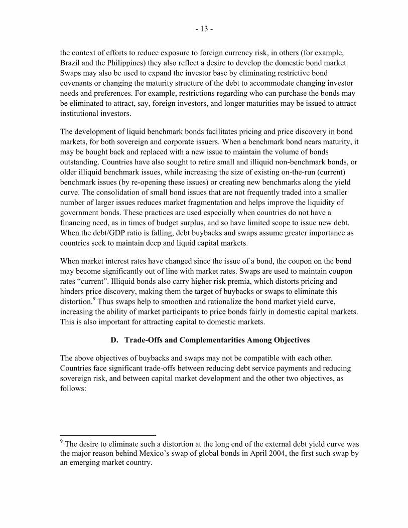
While external debt buyback and swap activity remains small relative to total external debt and to GDP, it has risen in recent years (Figure 1). There was a surge of activity in 2006: in the period January through November 2006, buyback and swap operations in a group of thirteen emerging market countries for which data are available rose to 5.3 percent of total external debt and 1.6 percent of GDP. The sharp increase in activity in 2006 reflected, in particular, liability management operations by Brazil and Russia to reduce debt service costs, lower sovereign risk, and develop domestic capital markets.

Repurchases of Brady bonds to lower debt service costs have been a major factor in the recent growth of debt buyback and swap activity.2 These bonds were issued beginning in 1990, and constituted a significant part of the total debt of many countries, especially in Latin America. They contained many exotic features reflecting the undeveloped state of the emerging market bond market and the limited access of countries to capital markets. However, as countries gained more access to capital markets and world interest rates fell, Brady bonds became relatively expensive. In addition, they tied up collateral. This prompted countries to reduce or eliminate their holdings of such bonds through buyback or swap operations, and outstanding Brady bond holdings declined from US$154 billion in 1994 to US$10.7 billion at mid-December 2006.

The literature on the principles of corporate bond refundings is sizeable. However, while sovereign debt buybacks and swaps have become increasingly important, there is little literature available on the role, functions, and mechanics of these operations that could serve as a guide to a sovereign debt manager in an emerging market or developing country. This paper seeks to fill this gap by examining the key conceptual and practical issues that a 2 Brady bonds—named after U.S. Treasury Secretary Nicholas Brady, who launched the initiative in 1989—were issued by some emerging market countries, particularly in Latin America, as part of a restructuring of defaulted commercial bank loans. The bonds were tailor-made in all sizes, and carried a wide variety of covenants, conditions, warrants, and other complex features, such as collateral.

- 4 -

government debt manager needs to take into account in the management of debt buyback and swap operations.

Figure 1: External Debt Buybacks and Swaps in Emerging Market Countries. 1/

Sources: IMF; Financial Times; Dow Jones Newswire; and Euroweek.

1/ Agregated data for Brazil, Bulgaria, Colombia, Ecuador, Lebanon, Mexico, Panama, Philippines, Poland, Russia, Turkey, Uruguay, and Venezuela.

0%

1%

2%

3%

4%

5%

6%

2003 2004 2005 2006 2/

Percent of GDPPercent of Total External Debt

The rest of the paper covers the macroeconomic context in which buybacks and swaps are undertaken (Section II), the objectives of buybacks and swaps (Section III), the analytical framework for deciding whether to undertake a particular buyback or swap operation and for selecting among alternative operations (Section IV), and some key issues in the determination of the strategy for executing buybacks and swaps (Section V). An appendix contains a numerical example of a hypothetical debt swap operation. Finally, the paper deals only with voluntary buybacks undertaken as part of routine liability management by the government, not with negotiated buybacks and swaps undertaken in the context of a debt restructuring.

- 5 -

II. MACROECONOMIC CONTEXT OF DEBT BUYBACK AND SWAP OPERATIONS

Debt managers need to understand the broader context of debt buyback and swap operations. The institutional framework of these operations falls into a broader category of the institutional framework of debt management, which is nested within a broad context of public policy aiming to maintain a sustainable level and growth rate of public debt. In this context, the aim of debt management is to raise the required funding for the government and attain the desired risk level, cost, and composition of the public debt. Debt management operations, of which buybacks and swaps are the two most important types, may also serve the purpose of developing and supporting the domestic capital market, especially the market for government debt instruments.

Debt buybacks and swaps have to be implemented under multiple macroeconomic constraints. These concern the condition of domestic and international capital markets, the exchange rate regime, the quality of macroeconomic policies, the regulatory environment (at home and in the international capital markets), the credit rating of the country, the objectives of the debt policy, and even the human and technological capacity to conduct debt management operations. In this light, the success of debt management operations relies on the consistency between debt policy and macroeconomic policies.

To ensure consistency between the two, debt management operations should be coordinated with fiscal and monetary policies. Prudent debt management and fiscal and monetary policies can act together and create a positive feedback in the attempt to lower debt costs, risk premia, and long-term interests rates, or to develop the domestic capital market. Inappropriate fiscal and monetary policies may result in a risky debt structure, that in turn may lead to an increased vulnerability of the domestic economy to economic and financial shocks. The same may happen if debt management practices are inappropriate, even if the macroeconomic policies are sound and coherent. However, prudent debt management practices cannot replace sound fiscal and monetary policies. Similarly, debt management operations alone cannot help develop local capital markets if fiscal and monetary policies are not supportive of this goal.

Debt buybacks and swaps have important implications for fiscal and monetary policies. Debt buybacks in the domestic market increase liquidity in the financial system. This, in turn, expands aggregate demand and may inflate domestic asset prices. This risk is higher in countries with less developed and illiquid capital markets. Buybacks of foreign currency debt in domestic and international capital markets, or swaps of foreign and domestic debt, directly affect foreign exchange reserves. If these operations are not taken into account when formulating monetary and fiscal policies, they may have undesirable consequences and will necessitate sterilization by the central bank. Sterilization can be costly, especially if it results in higher interest rates. Regardless of whether the central bank or the government ultimately bears the cost of sterilization, these costs can negatively affect the financial position of the public sector, and can at least partially cancel out the benefits of debt buybacks.

- 6 -

To strengthen the coordination between debt management and macroeconomic policies, some countries have integrated debt management into overall public sector risk management. This broader risk management framework includes government balance sheet analysis and asset-liability management (ALM). It allows debt managers to asses better the risks associated with government assets, or to compare the structure of the public debt with the government’s capacity to service this debt from revenues and other cash flows. Also, the ALM approach is useful in countries where foreign reserves are backed by borrowing in foreign currencies. In such a situation, debt management operations can aim to match the currency composition of the debt and the reserves. However, this approach can be limited by the independence of the central bank or the exchange rate regime.

III. OBJECTIVES OF DEBT BUYBACKS AND SWAPS

Debt managers need to be very clear on the objective underlying a debt buyback or swap operation. This may not be easy because, as will be seen below, the objectives are not mutually exclusive or necessarily compatible with each other. There are in general three core reasons why governments in emerging market countries undertake debt buybacks and swaps: to reduce debt service payments, to minimize sovereign risk, and to develop domestic capital markets. Sometimes countries have other objectives, such as releasing collateral and eliminating restrictive bond covenants, but these tend to be subsidiary to the main objectives.

These three core objectives are the link between sovereign liability management operations and the ultimate economic goals of the society. Attainment of these objectives helps strengthen fiscal and monetary policies, reduce a debt overhang that may be constraining investment and growth, and reduce a country’s external vulnerability. The final result is improved macroeconomic performance, higher domestic investment and growth, and prevention of financial crises, which are the ultimate economic goals of a society. In addition, buybacks and swaps, to the extent that they reduce the debt stock and debt service payments and stimulate investment and growth, may help lower future tax rates and boost the income of future generations.

The three core objectives constitute clear economic rationale for a debt buyback or swap operation. They are “sufficient” reasons for a country to consider engaging in such an operation because they are clearly justifiable in terms of their potential macroeconomic contribution and the attainment of the society’s broader economic goals—although, whether the operation is actually undertaken will depend on other criteria too, such as the costs of the operation, as discussed in Section IV. Objectives such as releasing collateral and eliminating restrictive bond covenants do not necessary provide by themselves clear economic criteria to justify a buyback or swap. They can only complement or reinforce the core objectives.

- 7 -

A. Reducing Debt Service Payments

Buybacks and swaps affect the size of the government’s debt service payments in any given time period through changes in the stock of government debt or in the average interest rate on the debt. Cash buybacks (which are financed through a drawdown of cash reserves or other liquid assets) lower the debt stock by the face value of the buyback, which results in a saving of interest on the debt bought back—and possibly of principal also if the debt was bought at a discount. Many countries buy back their debt when it is trading at a discount in the secondary market, to realize the principal savings. Secondary market purchases of discounted debt have in the past been advocated as one way of resolving a country’s debt overhang.3

Debt refunding (or refinancing) through a swap seeks to lower debt service payments by replacing high-coupon debt with lower-coupon debt.4 As already noted, this is a major reason why many countries have replaced or reduced their outstanding Brady bonds. Countries normally resort to refunding when interest rates have fallen. However, while swaps alter the interest rate on the debt, they do not necessarily leave the debt stock unchanged. Countries may choose to replace an existing bond issue with a larger issue, for example, in order to increase the liquidity of the issue or to cover the transactions costs of the swap. In such a case, the net impact on debt service payments will depend on the relative magnitudes of the interest rate effect and the debt stock (scale) effect.5

The assessment of the debt service impact of a cash buyback would need to take into account the opportunity cost of the funds used in the buyback, that is, any interest earnings foregone. Where domestic debt is bought back, the opportunity cost may be just the earnings on government deposits. Where foreign debt is bought back using net international reserves purchased from the central bank, an additional cost may be the difference between the central bank’s earnings on international reserves and its earnings on domestic assets.

3 During the sovereign debt crises in the 1980s some observers advocated debt buybacks as a solution to a country’s debt overhang, defined by Krugman (1988) as a situation in which the present value of potential future resources available to service the debt is less than the present value of the future debt service payments. This has stirred a debate on whether countries benefit from debt buybacks, and whether buybacks and swaps are effective in averting macroeconomic crises, which we do not go into in this paper. See, for example, Bulow and Rogoff (1998 and 1991), Dornbusch and others (1988), Thomas (1996), and Aizenman, Kletzer, and Pinto (2005). 4 This is called a high-coupon refunding. Replacement of low-coupon with high-coupon debt is referred to as low-coupon refunding. 5 However, in calculating the net benefit of a swap it is normally assumed that the face value of the debt remains unchanged. This is explained in Section IV.

- 8 -

In general, in principle the calculation of debt service impact should take into consideration any effects of the transaction on the government’s borrowing costs elsewhere in the economy (that is, general equilibrium effects). As mentioned previously, a buyback program may exert upward pressure on domestic bond prices, or may trigger sterilization by the central bank that would push up domestic interest rates, especially where bond markets are under-developed and illiquid. In practice, these general equilibrium effects may be difficult to trace and quantify and, therefore, difficult to incorporate in debt service calculations. Debt managers, however, should undertake at least a qualitative assessment of these effects. Such an assessment may be an important consideration where quantitative analysis indicates only a marginal net benefit of a buyback or swap.

Debt buybacks and swaps may also reduce the interest rate on future borrowing to the extent that they help improve a country’s creditworthiness and, therefore, result in credit rating upgrades and lower risk premia. The issue of credit ratings and capital market access is discussed below.

B. Reducing Sovereign Risk

A major objective of buyback and swap operations by emerging market governments is to reduce the risks inherent in a government’s debt portfolio. The risks encountered in sovereign debt management are described in Box 1. The main risks governments seek to lower are rollover risk, interest rate risk, exchange rate risk, and liquidity risk. To accomplish this objective, governments use buybacks and swaps to change the debt’s maturity structure, interest rate structure, and currency structure, and to improve access to international capital markets.

It should be noted that buyback and swap operations themselves do carry some sovereign risk6. These include the reputational risk that the operation may be unsuccessful, which could harm a country’s creditworthiness; the risk that both the refunding bond and the refunded bond may end up being illiquid if the swap does not attract sufficient investor interest; and the normal credit or operational risks associated with any transaction. These risks underscore the importance of careful selection and timing of buyback and swap operations, backed by sufficient due diligence regarding investor interest and demand.

6 See “Report on Bond Exchanges and Debt Buy-Backs: A Survey of Practice by EU Debt Managers” (2001).

- 9 -

Box 1: Risks Encountered in Sovereign Debt Management

Risk Description

Market Risk Refers to the risks associated with changes in market prices, such as interest rates, exchange rates, commodity prices, on the cost of the government’s debt servicing. For both domestic and foreign currency debt, changes in interest rates affect debt servicing cost on new issues when fixed rate debt is refinanced, and on floating rate debt at the rate reset dates. Hence, short-duration debt (short-term or floating rate) is usually considered to be more risky than long-term, fixed rate debt. (Excessive concentration in very long-term, fixed rate debt also can be risky as future financing requirements are uncertain.) Debt denominated in or indexed to foreign currencies also adds volatility to debt servicing costs as measured in domestic currency owing to exchange rate movements. Bonds with embedded put options can exacerbate market and rollover risks.

Rollover Risk The risk that debt will have to be rolled over at an unusually high cost or, in extreme cases, cannot be rolled over at all. To the extent that rollover risk is limited to the risk that debt might have to be rolled over at higher interest rates, including changes in credit spreads, it may be considered a type of market risk. However, because the inability to roll over debt and/or exceptionally large increases in government funding costs can lead to, or exacerbate, a debt crisis and thereby cause real economic losses, in addition to the purely financial effects of higher interest rates, it is often treated separately. Managing this risk is particularly important for emerging market countries.

Liquidity Risk There are two types of liquidity risk. One refers to the cost or penalty investors face in trying to exit a position when the number of transactors has markedly decreased or because of the lack of depth of a particular market. This risk is particularly relevant in cases where debt management includes the management of liquidity assets or the use of derivatives contracts. The other form of liquidity risk, for a borrower, refers to a situation where the volume of liquid assets can diminish quickly in the face of unanticipated cash flow obligations and/or a possible difficulty in raising cash through borrowing in a short period of time.

Credit Risk The risk of nonperformance by borrowers on loans or other financial assets or by a counterparty on financial contracts. This risk is particularly relevant in cases where debt management includes the management of liquid assets. It may also be relevant in the acceptance of bids in auctions of securities issued by the government, as well as in relation to contingent liabilities, and in derivative contracts entered into by the debt manager.

Settlement Risk Refers to the potential loss that the government, as a counterparty, could suffer as a result of failure to settle, for whatever reason other than default, by another counterparty.

Operational Risk

This includes a range of different types of risks, including transactions; inadequacies or failures in internal controls, or in systems and services; reputation risk; legal risk; security breaches; or natural disasters that affect business activity.

Source: IMF and World Bank (2003)

- 10 -

Changing the Maturity Structure

Emerging market countries often alter the maturity structure of their existing debt for two reasons. First, they may lengthen the average maturity or duration of the debt, and second, they may smooth (flatten) the debt service (particularly the redemption) profile to better match the government’s steady flow of revenues. In an asset-liability management framework, a longer average maturity of the debt and a smoother debt service profile better match the generally long-term nature of the government’s assets and revenue flows, and reduce duration risk. Duration risk may materialize as a liquidity or rollover crisis. The maturity structure of the debt is therefore a crucial consideration in asset-liability management.

Shorter-term debt is also inherently more susceptible to market and rollover risk, which increases a country’s vulnerability to rising interest rates and unfavorable currency movements. These risks are particularly important where capital markets are shallow and illiquid. Since domestic capital markets in many emerging market countries are not deep enough, short-term domestic debt in these countries is particularly subject to market and rollover risk. Countries therefore try to avoid a bunching of short-term maturities, especially of domestic debt.

Changing the maturity structure of the debt involves buying back bonds or replacing them with bonds of a different maturity. In a swap, usually the refunding bonds are of longer maturity than the refunded bonds, to lengthen the average maturity and duration of the debt. Swaps may also be used to create better spacing of bullet amortizations, to lessen the lumpiness in the debt service profile, or to replace such amortizations with sinking fund debt to spread the principal repayments over time. Lengthening the maturity of the debt also pushes debt service payments into the future, which provides temporary relief from short-term budgetary pressures and reduces rollover risk.

When used for short-term budget relief in this way, swaps effectively become cash management rather than debt management tools for the government. This blurs the distinction between debt management and the financing operations of the government. In the absence of such short-term financing pressures, alteration of the maturity profile of the debt is part of routine liability management by governments to satisfy their financing needs at the minimum of cost and risk.

Changing the Interest Rate and Currency Structures

Floating interest rate debt, foreign currency debt, and foreign-currency-linked debt are major sources of vulnerability in many emerging market countries. A significant share of the debt of these countries is exposed to the risk of interest rate or currency shocks. As has been

- 11 -

pointed out by others7, floating rate and foreign currency debt may create balance sheet mismatches to the extent that the government’s revenues (for example, its domestic revenues) or other cash inflows are not linked to interest rates and the exchange rate. As such, unfavorable interest rate or exchange rate movements could create financial pressures, resulting in liquidity and rollover risk.

An important objective of debt management in many emerging market countries is to reduce interest rate and exchange rate risk by swapping floating rate debt for fixed-rate debt, and foreign-currency or foreign-currency-linked debt for domestic-currency debt. The increase in the ratio of fixed-rate to floating-rate debt and of domestic-currency to foreign-currency debt reduces the sensitivity of debt service payments to interest rate and currency shocks.

For most countries, the reduction of exchange rate risk involves retiring foreign and foreign exchange-linked debt and re-issuing domestic-currency debt in the domestic capital market. The extent to which countries can do this is limited by the size and liquidity of their domestic capital markets and, therefore, the scope for this kind of swap may be limited. This is the problem of “original sin” noted in the literature on financial crises8. Some countries, such as Colombia in 2004 and Brazil in 2005, have sought to overcome this constraint by issuing domestic currency debt in international capital markets. The success of these operations has been facilitated by the recent shrinking supply of emerging market foreign debt in an international environment marked by substantial liquidity and low yields. As macroeconomic fundamentals and debt management policies in emerging market countries strengthen, and sovereign credit ratings improve, more countries may be able to issue domestic currency debt abroad in the future. Emerging market countries have also been making efforts to improve their sovereign credit ratings and develop their domestic capital markets in order to attract foreign creditors to domestic markets.

Some countries have sought to change the foreign currency composition of the debt, switching to debt in currencies that reflect their trade links, or have used currency and interest rate swaps to hedge rather than eliminate the currency and exchange rate risk. For example, Bulgaria undertook a dollar/euro swap with the World Bank in November 2003. However, the scope for such swaps is limited by the lack of development of derivative markets in emerging market countries. In any event, currency and interest rate mismatches are long-term structural problems that may involve a substantial portion of the government’s debt, and cannot be permanently resolved by limited and short-term derivative operations. Their resolution requires a concerted liability management strategy.

7 See, for example, IMF and World Bank (2003), and Wheeler (2004). 8 The inability of countries to issue debt in domestic currency has been referred to as “original sin.” See, for example, Hausmann and Panizza (2003).

- 12 -

Maintaining and Expanding Access to International Capital Markets

Some countries, such as Mexico and Brazil, have used buybacks and swaps to enhance their international creditworthiness and improve their sovereign credit ratings, and thereby maintain or expand their access to international capital markets and lower their credit spreads. Maintaining or expanding access to capital markets ensures that financing gaps will be closed at acceptable costs to the government, increases a country’s financing options (for example, the ability to issue local-currency bonds in international capital markets, as noted above), and serves as insurance against liquidity and rollover risks. It also benefits corporate borrowers by expanding their market access and lowering their credit spreads, and by providing benchmarks for corporate issuance.

Frequent and successful buybacks and swaps help raise a country’s profile in international capital markets. To the extent that they improve debt and fiscal sustainability, they also enhance the government’s international creditworthiness. Buybacks and swaps may also be used to expand the investor base in international markets and build investor loyalty by maintaining the liquidity of foreign bonds, changing the maturity profile of the debt in line with evolving investor demand, and removing distortions in the foreign yield curve. These operations are similar to those used to develop domestic capital markets, and are explained below.

However, to improve their profiles as borrowers, countries need to select and time their operations carefully. As noted above, an unsuccessful operation may harm the government’s reputation and lower its creditworthiness. Also, the re-purchase of domestic government debt held by public sector agencies, such as the social security institute, would not improve the net fiscal balance of the public sector because intra-sector transactions would be netted out. This kind of re-purchase probably would not have any effect on a country’s creditworthiness. To enhance creditworthiness by improving the public finances, buybacks should target domestic debt held by the private sector or external debt.

C. Developing Domestic Capital Markets

Emerging market countries seek to develop their domestic capital markets for a variety of reasons, including the expansion of domestic borrowing opportunities to reduce the dependence on foreign borrowing and the exposure to exchange rate risk. Buybacks and swaps have been used in three ways to help achieve this objective, namely: to increase liquidity in domestic markets, to develop benchmark bond issues, and to smooth and rationalize the bond yield curve. In addition, the use of buybacks and swaps helps develop the capital market infrastructure—for example, reverse auction mechanisms and the clearing and settlement system.

The volume of bonds traded is a key determinant of liquidity in domestic bond markets. Swaps of domestic for foreign bonds increase the domestic supply of bonds, which attracts capital to the domestic market. Though in some countries these operations are undertaken in

- 13 -

the context of efforts to reduce exposure to foreign currency risk, in others (for example, Brazil and the Philippines) they also reflect a desire to develop the domestic bond market. Swaps may also be used to expand the investor base by eliminating restrictive bond covenants or changing the maturity structure of the debt to accommodate changing investor needs and preferences. For example, restrictions regarding who can purchase the bonds may be eliminated to attract, say, foreign investors, and longer maturities may be issued to attract institutional investors.

The development of liquid benchmark bonds facilitates pricing and price discovery in bond markets, for both sovereign and corporate issuers. When a benchmark bond nears maturity, it may be bought back and replaced with a new issue to maintain the volume of bonds outstanding. Countries have also sought to retire small and illiquid non-benchmark bonds, or older illiquid benchmark issues, while increasing the size of existing on-the-run (current) benchmark issues (by re-opening these issues) or creating new benchmarks along the yield curve. The consolidation of small bond issues that are not frequently traded into a smaller number of larger issues reduces market fragmentation and helps improve the liquidity of government bonds. These practices are used especially when countries do not have a financing need, as in times of budget surplus, and so have limited scope to issue new debt. When the debt/GDP ratio is falling, debt buybacks and swaps assume greater importance as countries seek to maintain deep and liquid capital markets.

When market interest rates have changed since the issue of a bond, the coupon on the bond may become significantly out of line with market rates. Swaps are used to maintain coupon rates “current”. Illiquid bonds also carry higher risk premia, which distorts pricing and hinders price discovery, making them the target of buybacks or swaps to eliminate this distortion.9 Thus swaps help to smoothen and rationalize the bond market yield curve, increasing the ability of market participants to price bonds fairly in domestic capital markets. This is also important for attracting capital to domestic markets.

D. Trade-Offs and Complementarities Among Objectives

The above objectives of buybacks and swaps may not be compatible with each other. Countries face significant trade-offs between reducing debt service payments and reducing sovereign risk, and between capital market development and the other two objectives, as follows:

9 The desire to eliminate such a distortion at the long end of the external debt yield curve was the major reason behind Mexico’s swap of global bonds in April 2004, the first such swap by an emerging market country.

- 14 -

• increasing the average maturity of the debt, or switching from floating-rate to fixed-rate debt, will normally increase the cost of the debt given that long-term interest rates are usually higher than short-term rates;

• switching from foreign currency or foreign currency-linked debt to domestic currency debt, either in domestic or international capital markets, may increase the cost of the debt because of higher interest rates and higher risk premia stemming from less liquid domestic capital markets, inflation risk if macroeconomic policies are not seen to be appropriate, and lower confidence in the domestic currency; and

• switching from foreign to domestic debt may involve a trade-off between foreign exchange risk and rollover risk, given that short-term and floating rate debt may be the only type of debt the government can issue in less developed domestic capital markets.10

The magnitude of the trade-offs depends on market conditions and the structure of the debt. These include:

• the slope of the yield curve: the steeper the curve (assuming a normal, positive slope), the larger will be the impact on debt service of lengthening the maturity of the debt or switching from floating rate to fixed-rate debt;

• the size of risk premia: the larger the risk premium that is paid in accomplishing the swap, as may be the case when switching from foreign currency or foreign currency-linked debt to domestic currency debt or when lengthening the maturity of the debt in a situation of possible default, the larger will be the impact on debt service;

• the average maturity of the debt stock: the shorter the maturity of the debt, the larger is the rollover and liquidity risk and the larger will be the impact on sovereign risk, at the margin, of any given debt swap; and

• the share of foreign-currency or foreign-currency-linked debt and floating-rate debt in the total debt stock: the larger this share, the larger will be the impact on sovereign risk, at the margin, of a switch from this kind of debt to domestic-currency or fixed-rate debt.

However, there may be complementarities among the objectives; that is, the attainment of one objective may help to achieve one or more of the other objectives. In the short run, there may be a complementarity between risk reduction and capital market development if the trade-off between exchange rate and domestic rollover risk is favorable, or if there is little or no rollover risk associated with domestic capital markets. In the long run, there is a complementarity between cost and risk reduction and capital market development, since the latter should result in a reduction in liquidity and rollover risk premia.

10 See: IMF and World Bank (2003), page 26, paragraph 83.

- 15 -

Any prospective buyback or swap has to take into consideration the tradeoffs and complementarities involved in the transaction, and debt managers will need to assess the nature and magnitude of these where possible. Put differently, every buyback or swap operation leaves the debt portfolio with particular cost and risk attributes, and the capital market in a particular state of development. The crux of buyback and swap evaluation is to determine the combination of cost, risk, and capital market attributes that is associated with the buyback or swap, and whether this combination is superior to the one existing without the buyback or swap, or to the combination that is associated with any other buyback or swap operation that could be undertaken for the same purpose. The procedures to conduct such an evaluation are discussed in Section IV.

IV. ANALYTICAL FRAMEWORK FOR SELECTING BUYBACKS AND SWAPS

There are three necessary conditions for a debt manager to undertake a particular buyback or swap in any given moment in time. First, the operation must accomplish its intended or primary objective (as discussed below). This condition is obvious, but determining whether or not it is satisfied may be difficult in practice. It requires that debt managers have clear objectives and decision rules. Second, the operation either must not impact unfavorably on any other objective, or, if it does, that other objective is of secondary importance or lesser priority. This condition requires that debt managers explicitly take into account the trade-offs and priorities among objectives, to ensure that the impact of the operation is properly measured and evaluated. Third, the buyback or swap under consideration must contribute more to the attainment of the intended objective than any other buyback or swap that could be undertaken for the same purpose. This condition ensures that resources are put to their most productive use at any given moment in time. It requires that debt managers rank the different buybacks and swaps that could be undertaken to achieve a given objective.

In determining whether these three conditions are satisfied, the debt manager must answer five questions about the buyback or swap operation. These five questions are posed in Section IV.A, roughly in the order in which they should be answered. This results in a sequential decision-making process, which leads in the end to a decision on whether any particular buyback or swap should be undertaken. A summary and overview of the decision-making process in presented in Section IV.B.

A. Five Questions for the Debt Manager

What is the Objective of the Operation?

Any individual buyback or swap should preferably have a single, clearly-defined, objective, which we shall call the intended objective of the operation. This follows the general principle that a single instrument should not be used to pursue multiple objectives. Where multiple objectives are sought, more than one buyback or swap operation should be used. For example, one operation can target a reduction in debt service payments and another can

- 16 -

target a reduction in risk. This makes it easier to evaluate a buyback or swap, frees the debt manager to undertake the best strategy in each case to achieve the desired objective, and avoids a situation where a single operation is trying to achieve conflicting objectives. For example, to reduce foreign exchange risk, the country may wish to develop its capacity to issue local currency bonds in international capital markets. This may be preferable, because of cost or other considerations, to the issuance of bonds in domestic capital markets. In this case, a second operation can be used to target capital market development.

However, there may be times when it may be possible to pursue multiple but complementary objectives with a single buyback or swap—for example, capital market development and a reduction in foreign exchange risk. In these situations, one of the objectives should be designated the primary (intended) objective and any favourable impact on the other objectives should be viewed as external (unintended) benefits of the operation. This simplifies the evaluation of the operation, especially the comparison of alternative ways of achieving the same objective. The buyback or swap manager should be very clear as to the intended benefit or rationale of the operation. External benefits and costs should also enter the decision-making process, and will influence the final decision to undertake or not the operation, as will be seen below; but consideration of external benefits and/or costs is a separate and distinct aspect of the decision-making process that should not confuse the assessment on the basis of the intended objective.

Will the Operation Achieve its Intended Objective?

In principle, a debt buyback or swap decision is best viewed as an investment decision. It brings a future stream of benefits—net savings in interest payments, a reduction of sovereign risk, or the benefits of capital market development—in return for certain investment costs. The costs may be incurred today (such as transactions costs or cost of the bond buyback) or in the future (such as interest foregone in the case of a cash buyback). A non-negative net present value (NPV) (or internal rate of return) of these benefits and costs would be a necessary, but not sufficient, condition for the buyback or swap to be undertaken, as will be seen. This is a capital budgeting approach to buyback and swap decision-making.

In practice, this approach is most readily applied if the objective is to reduce debt service payments, because in this case there are well-defined direct benefits and costs of the operation that can be quantified. The direct benefits of a swap, say, that leaves the principal outstanding unchanged would be the saving in future interest payments (difference between coupon rates of the old and the new bonds). The direct costs would include the cost of the bond bought back and the transactions costs. These benefits and costs can be estimated—although the estimation may be difficult if interest and exchange rates are floating—and the net present value calculated. The application of this procedure to determine the net financial benefit of a buyback or swap operation is described in Section C below.

- 17 -

When the objective is to reduce sovereign risk or to develop the domestic capital market, however, quantification of the benefits of the operation may be very difficult or impossible. The benefit of a reduction of rollover risk, for example, by lengthening the average maturity of the debt, is a reduction in the probability of default on the debt. The financial and economic consequences of default—loss of investment, output, and employment and higher financing costs, for example—are hard to quantify. The same is true for capital market development, such as expanding liquidity and lengthening yield curves, which provides general economic and financial benefits. Net present value calculations to determine if a risk or capital market objective will be achieved are therefore not practical.

For these two objectives, a second-best procedure would be to determine a desired structure of the government’s debt and evaluate buybacks or swaps according to whether or not they help to attain this desired structure. This desired structure may be considered the optimal structure of the debt from the government’s perspective, and would be defined in terms of quantitative indicators that serve as measures of risk or capital market development. Risk indicators could include, for instance, average term to maturity of the total debt, the ratio of fixed-to-floating debt, and the ratio of foreign-currency to domestic-currency debt. Indicators of capital market development could include the ratio of domestic debt to GDP and average term to maturity of the domestic debt. The government would establish targets or benchmarks (called strategic benchmarks) for one or more of these indicators, which then define the optimum structure of the debt as determined by the government. Individual buybacks or swaps are evaluated according to whether they help achieve these targets or benchmarks. The strategic bookmarks are discussed in Section IV.D. below.

What Are the Trade-Offs and Complementarities?

The tradeoffs and complementarities among objectives would be assessed according to the procedures just described. If the intended objective is to reduce debt service payments, then the debt operation’s unintended impact on the structure of the debt would need to be evaluated using the established strategic benchmarks. This would indicate how sovereign risk or capital market development is affected by the operation. Similarly, if the objective is to bring the structure of the debt closer to the desired structure as defined by the strategic benchmarks, then the budgetary impact should be assessed using the net present value approach.

Effectively, as mentioned above, the buyback or swap should be evaluated from the perspective of all three objectives. This will enable the debt manager to determine how the buyback or swap will affect the portfolio’s cost and risk attributes and the state of capital market development. Such a comprehensive view of the operation is essential to arrive at the correct decision on whether or not the operation should be undertaken.

- 18 -

Do the Trade-Offs and Complementarities Affect the Decision?

Once the trade-offs involved in any prospective operation are objectively assessed, they must be evaluated in light of the government’s (or the society’s) priorities among the different objectives. On the basis of this evaluation, the government decides whether the trade-offs involved in the prospective operation are acceptable or not. An acceptable trade-off is a necessary condition to proceed with the buyback or swap operation. Complementarities (unintended benefits) reinforce the positive net direct benefits of the operation and strengthen the case for proceeding with the operation. Put differently, in this phase of the analysis the government decides if the combination of portfolio cost and risk and capital market attributes associated with the buyback or swap is superior (preferable) to the one that would exist without the buyback or swap. If it is, then the condition is satisfied to proceed with the next phase of the analysis.

To answer the question posed, debt managers need to have clear-cut priorities among the different objectives. The intended objective of the debt operation may not necessarily be the objective with the highest priority, in which case the debt manager may decide not to undertake the operation, even if it would achieve its objective, if it adversely affects the attainment of a higher-priority objective. For example, a country may undertake routine debt swaps to maintain or increase the liquidity of benchmark bond issues. Should such swaps be undertaken if they result in higher financing costs for the government, as, for example, in cases where the interest rate on the new bond would be higher than that on the old bond? The answer to this question depends on the country’s circumstances at the time, such as the stance of fiscal policy and the impact of the swap on the capital market. On the other hand, the government may well decide that the benefit of capital market development in this case does not justify the additional cost to the budget. On the other hand, if a country is facing a liquidity crisis and possible default, swaps to lengthen the maturity of the debt may be undertaken even if they result in higher interest payments in the future.

The priorities among cost, risk, and capital market development are not permanently fixed. They depend, among other things, on the government’s preference for risk, the state of the public finances, the risk characteristics of the debt portfolio, and the level of capital market development. These conditions will vary over time, and so will the priorities. The absolute size of the debt stock is also important, because the country’s vulnerability to interest rate and exchange rate shocks varies directly with the size of the debt. As the debt gets larger, cost and risk considerations become increasingly important and might take precedence over capital market considerations.

What is the Ranking of the Buyback or Swap?

Once it has been ascertained that a prospective buyback or swap operation will achieve its intended objective and cannot be rejected because of unfavorable trade-offs, the operation must then be ranked against other buyback or swap operations that can also achieve the intended objective. (These alternative operations must also be evaluated using the procedures

- 19 -

described above.) The operation under consideration may have a higher return, in terms of its intended objective, than alternative operations, but may have higher costs (adverse trade-offs) in terms of the other objectives. In other words, the debt manager has to choose between different operations that have different combinations of portfolio cost and risk and levels of capital market development associated with them. These different operations have to be ranked somehow according to their order of priority, and the one with the highest priority is selected for execution. This subject is discussed in Section E below.

The ranking of the different combinations of portfolio cost and risk and capital market development may be a straightforward matter at certain times, but may be highly subjective at other times. When the country is facing a short-term fiscal or financial difficulties, the nature of these difficulties may readily dictate the priorities. On these occasions, cost or risk considerations may be of paramount importance. Under normal conditions, however, when a debt operation is driven by routine debt management and not by such difficulties, there may be no objective way of choosing among different buyback and swap operations that offer different combinations of cost, risk, and capital market development. The implication of this is that debt managers need to operate under the general guidance of the policymakers, since the ranking of different debt operations at times may depend largely on the subjective preferences of the government.

B. Illustration of the Decision-Making Process

The sequential procedure described above is illustrated in Figure 2. It is assumed that the intended objective of the buyback or swap is to reduce the government’s debt service costs (but any other objective could have been taken as the starting point) by, say, swapping a high-coupon bond for a low-coupon one. The question is whether the operation should be undertaken or not.

With a non-negative NPV and no adverse effects on portfolio risk and/or capital market development, or with adverse effects that are acceptable to the government, the operation would be tentatively accepted at stage 3 of the exercise (left half of Figure 2). Final acceptance at stage 4 would depend on the operation’s ranking vis-à-vis other buybacks or swaps that could be undertaken to lower debt service costs. If there are adverse risks and/or capital market effects that are considered more important than cost, the operation would be rejected at stage 3.

Conversely, with a negative NPV and no favourable effects on risk and/or the capital market, or with favorable effects that are subordinated to cost considerations, the operation would clearly be rejected at stage 3 (right half of Figure 2). It could only be accepted if any favorable effects on risk and/or the capital market are deemed to be more important than cost considerations. Note that, if the objective is cost reduction and the NPV is negative, one would expect the operation to be rejected at Stage 3 even if there are favorable risk and/or capital market effects. If the operation with a negative NPV is accepted on the grounds that it

- 20 -

helps achieve the other objectives, this would be tantamount to saying that the intended objective of the operation is really risk or capital market development, not cost reduction. In such a case, as seen in Figure 2, in Stage 4 the relevant alternatives to consider would be those that could help achieve the risk or capital market objective, not those that necessarily lower debt service payments.

C. Measuring the Net Financial Advantage of a Buyback or Swap Operation

This section sets out the procedure for calculating the net financial advantage (benefit) of a sovereign debt buyback or swap, drawing on the well-developed body of literature on corporate bond refundings.11 The principles of corporate refundings can be readily applied to sovereign buybacks and swaps. A major difference is that tax considerations influence corporate refunding decisions, whereas they are irrelevant (from the sovereign’s perspective) in a sovereign debt operation. Swaps are discussed first, then buybacks.

The Net Financial Advantage of a Swap

To calculate the net financial advantage (net advantage) of a swap, it is assumed that the existing (old or refunded) bond is replaced by a non-callable bond (the new or refunding bond) of identical maturity and par value. Only the coupon rate is different. The assumption of identical maturity and par value is standard in the literature on corporate bond refundings. Its rationale is the need to prevent differences in the maturity of the bonds and the principal outstanding from influencing the NPV calculations and therefore the net advantage of the operation. Since the financial objective of a swap is normally to reduce interest payments, the merits of the swap should be judged entirely by the impact on interest costs. The assumption that the new bond is non-callable means that the market value of the bond can be calculated as the sum of the present values of the future cash flows; this cannot be done for a callable bond because in this case the market value will be constrained by the call premium on the bond and is not necessarily equal to the discounted sum of the cash flows. This assumption will simplify the analysis of the net advantage.

11 Finnerty and Emery (2001), particularly Chapter 10, provide a good description of the procedure for evaluating corporate bond refundings. See also Bowlin (1966) and Boyce and Kalotay (1979).

21

Figu

re 2

: Illu

stra

tion

of th

e D

ecis

ion-

Mak

ing

Proc

ess

St

age

1: W

ill th

e op

erat

ion

achi

eve

its in

tend

ed o

r prim

ary

obje

ctiv

e?

(Is t

he N

PV n

on-n

egat

ive)

?

Stag

e 2:

Are

ther

e an

y ad

vers

e ef

fect

s on

risk

and/

or c

apita

l m

arke

t dev

elop

men

t?

Stag

e 2:

Are

ther

e an

y fa

vora

ble

effe

cts o

n ris

k an

d/or

cap

ital

mar

ket d

evel

opm

ent?

No

Yes

Yes

N

o

Stag

e 3:

Are

the

adve

rse

risk

and/

or

capi

tal m

arke

t eff

ects

acc

epta

ble?

St

age

3: A

re th

e fa

vora

ble

effe

cts o

n ris

k an

d/or

cap

ital

mar

ket d

evel

opm

ent m

ore

impo

rtant

than

cos

t?

Yes

N

oY

esN

o

Stag

e 4:

Is th

e op

erat

ion

rank

ed a

bove

oth

er o

pera

tions

with

non

-neg

ativ

e N

PV?

Stag

e 4:

Is th

e op

erat

ion

rank

ed a

bove

oth

er o

pera

tions

that

cou

ld a

lso

achi

eve

the

risk

and/

or c

apita

l mar

ket o

bjec

tive?

Acc

ept

oper

atio

n A

ccep

t op

erat

ion

Rej

ect

oper

atio

n A

ccep

t op

erat

ion

Rej

ect

oper

atio

n

Rej

ect

oper

atio

n

Yes

N

o

Acc

ept

oper

atio

n R

ejec

t op

erat

ion

Acc

ept

oper

atio

n R

ejec

t op

erat

ion

Yes

N

oY

esN

o

22

The assumption that the maturity and par value of the new and old bonds are the same is made purely for analytical purposes. In practice, they may be different. As Finnerty and Emery (2001) note, once the decision has been made to go ahead with the refunding (swap), the actual transactions can be different from the hypothetical prescriptions used in the decision-making process. Also, the simplest swap to analyse is a domestic-currency fixed-fixed rate one, because the cash flows are more predictable. The basic principles will be explained first using this kind of swap. Floating rate and foreign currency debt introduce considerable uncertainty regarding the future cash flows, which makes the calculation much more difficult; they will be discussed after. Finally, the success of the swap will depend in part on the extent of bond-holder participation; this is another source of uncertainty regarding the impact of the swap on future cash flows. Again purely for decision-making purposes, it is assumed that there is 100 percent bond-holder participation in order to correctly calculate the net advantage of the swap.

The decision-making procedure involves identifying, quantifying, and discounting the stream of financial benefits and costs of the swap to determine the net present value or internal rate of return of the operation. Benefits are cash inflows, while costs are cash outflows. These inflows and outflows are identified below, and then the choice of the discount rate is discussed.

Benefits or cash inflows

Saving of principal payment on the old bond. This is equal, in nominal terms, to the face value of the old bond, F, which is due to be paid in period T (in a single lump sum) when the bond matures.

Saving of interest payments on the old bond. The nominal interest due in any period, t, is rF, where r is the coupon rate on the old bond.

Net proceeds from the sale of the new bond. It is assumed that the new bond is fairly priced—that is, the coupon rate on the bond is equal to the market yield at the time of issue, inclusive of any risk premium. Thus the market value of the new bond is equal to the par value, and the bond is issued at par value, which, by assumption, is equal to F, the par value of the old bond. At times the new bond may command a discount. Such a discount would be treated as a transactions cost of the operation, and is covered below. Conversely, if the new bond is issued at a premium, the premium would be an inflow that would be netted out from the transactions costs.

Costs or cash outflows

Re-purchase price of the old bond. This is the cost, E, of retiring the old bonds. If a call option were being exercised, E would be the call price of the bond determined by the bond indenture, which may not be equal to F.

23

Principal repayment of the new bond. This amount is equal to F, the par value of the old bond, and is due in period T (in a single lump sum) when the bond matures.

Interest payments on the new bond. The nominal interest due in any period, t, is r'F, where r' is the coupon rate on the new bond. By assumption that the bond is fairly priced, r' is the rate that would make the new bond sell at par value. As noted above, r' is the market yield inclusive of any risk premium. If the actual yield is not equal to r' (the bond is issued at a discount or premium), the transactions cost of the swap is adjusted to reflect the discount or premium.

Transactions costs. These are incidental costs, A, that are necessary to complete the swap operation. They include:

• cost of floating the new bond, such as underwriting commission, lawyers and accountants fee, and printing costs;

• cost of retiring the old bonds, including any cost of printing redemption notices and any fees to the bond trustees for cancelling the old bonds;

• overlapping interest, which is any interest paid on the new bonds prior to the retirement of the old bonds, less any interest earned on the proceeds of the new bonds during the period of overlap;

• accrued interest on the old bonds, if the redemption date is different from a coupon payment date; and

• discount or premium on the issue of the new bonds, with a discount being a cost and a premium (which is a cash inflow) entering with a negative sign.

The discount rate

The standard practice in the literature on corporate bond refundings is to use the interest rate on the new bond as the rate of discount for all cash flows in the operation. The rationale for this is that the opportunity cost of the refunding is the cost of the new debt. In other words, conceptually the discount rate is the opportunity cost of the funds used to finance the buyback of the old bond. This is the same principle used in the cost-benefit evaluation of investment projects. As mentioned earlier, a sovereign bond buyback or swap operation can be viewed as an investment project, which means that its cash flows should be discounted using the opportunity cost of the financing. Hence, for sovereign bond refundings also the correct discount rate to use is r'.

However, it may be difficult to determine ex ante the cost of the new debt. To overcome this difficulty, the interest rate on the new debt may be estimated using the existing yields on debt of similar type and quality, issued either by the government or by other governments with similar credit ratings within the same region. It is assumed below that r' can be estimated in this way.

24

An alternative approach to the discounting procedure is to calculate the break-even discount rate by setting the NPV equal to zero and calculating the interest rate that would make the sum of the discounted cash flows equal to zero. This break-even rate is the internal rate of return (IRR) of the operation. Actual interest rates below the IRR would result in a positive NPV, while interest rates above the IRR would produce a negative NPV. The advantage of this approach is that the government can still take a decision on the debt swap even if it does not have a precise idea of the interest rate on the new bond—all it needs to do is determine that the interest rate on the new bond will fall below the break-even rate. The IRR approach is equivalent to the NPV approach. However, the NPV approach is discussed below because this is the more common procedure.

The net advantage of the swap with fixed interest and exchange rates

Combining the above elements leads to the following expression for the net advantage, Q, of the swap:

AFr

FrFrE

rF

rrFQ T

T

ttT

T

tt −⎥

⎦

⎤⎢⎣

⎡−

′++

′+′

−⎥⎦

⎤⎢⎣

⎡−

′++

′+= ∑∑

== )1()1()1()1( 11

(1)

The first term in square brackets is the present value of the savings in debt service costs of the old bond minus the re-purchase price of the old bond, the second term in square brackets is the present value of the debt service costs of the new bond minus the issue price of the new bond, and the last term is the transactions cost. Note that the cash flows of both the old and the new bond are discounted using the interest rate of the new bond. Equation 1 is simply the sum of all the cash inflows and outflows enumerated above. The swap is profitable to the government if the sum of all these flows, Q, is positive.

Since the new bond is assumed to be non-callable, it’s price, F, is given by the following expression:

T

T

tt r

FrFrF

)1()1(1 ′++

′+′

= ∑=

(2)

This means that the second term in square brackets in equation 1 is equal to zero, and the equation thus reduces to the following:

AEr

Fr

rFQ T

T

tt −−

′++

′+= ∑

= )1()1(1

(3)

In other words, the net advantage of the swap is the sum of the present values of the savings in debt service costs of the old bond minus the re-purchase price of the old bond minus the transactions costs of the swap. This can be written more compactly as follows:

25

AEVQ old −−= (4) If the old bond does not have a call option, oldV would be the market value of the bond, calculated using the yield on the new bond, and E may or may not be the market value also. If the bond has a call option that is being exercised, oldV would be the underlying market value of the bond (the market value if the bond did not have the call option), E would be the strike price of the bond, and EVold − would be the intrinsic value of the call option to the government. Thus, in the case of a bond with a call option, the net advantage of the swap is the intrinsic value of the call option minus the transaction costs.

Several things should be noted about equation 3 and 4. First, the cash flows of the new bond do not enter in equation 3. Effectively, the only role of the new bond in the decision-making process is to determine the discount rate. Thus, apart from the interest rate, the new bond may be disregarded entirely in the analysis. By equation 4, the swap is advantageous if the actual or underlying market value of the old bond, calculated using the yield on the new bond, exceeds the purchase price of the bond and the transactions costs; that is, if

AEVold +≥ (5)

Equation 5 is a necessary condition for proceeding with the swap.

Second, for a swap to be advantageous, there must be a minimum transfer of wealth from bondholders to the government. This can be seen by re-arranging the terms in equation 5:

AEVold ≥− (6)

EVold − in this equation is a transfer of wealth from bondholders to the government. For the swap to be profitable to the government, this transfer of wealth must be at least sufficient to cover the transactions costs of the swap. Naturally, the requirement that there be a transfer of wealth from bondholders would render the swap unattractive to bondholders, which may result in little or no bondholder participation in the swap if it is conducted on the secondary market. Thus a secondary market swap might not be successful even if it has a positive NPV from the government’s perspective.

Third, the swap is more likely to be successful if it involves the exercise of a call option on the old bond. For a bond with a call option, the purchase price is fixed by the bond indenture, and bondholders are forced to sell. The government can time the swap so as to ensure that the required minimum transfer of wealth from bondholders takes place. To facilitate the timing of the transaction, the break-even bond interest rate can be calculated. As noted above, this is the interest rate that would make the NPV of the swap equal to zero. The swap will be profitable if the current bond rate is less than the break-even rate. If interest rates are falling, the government can increase its profits by postponing the call of the bond. Mathematical

26

techniques exist to forecast interest rates and help determine the best timing point for the exercise of the call option. A discussion of these techniques is beyond the scope of this paper.

The net advantage of the swap with floating interest and exchange rates

The introduction of floating interest and exchange rates does not affect the basic methodology for computing the net advantage of the swap, but makes the calculation more difficult because it involves forecasting the interest and exchange rates in order to quantify the cash flows. It also implies that the discount rate will change over time if the interest cost of the new debt changes. Floating interest rates are considered first while still holding the exchange rate fixed, and then floating exchange rates are introduced.

In a fixed-to-floating rate swap, the only change in the above analysis would be that the discount rate, r', in equation 3 would need to be adjusted from period to period as the interest rate on the new debt is adjusted at the start of each fixing period. As can be seen from equation 3, the rest of the cash flows will remain unchanged. On the other hand, in a floating-to-fixed rate swap, the discount rate is unaffected (it remains fixed throughout) but the interest rate, r, and hence the saving in interest cost, rF, in equation 3 will vary from period to period. Finally, in a floating-to-floating rate swap, both r' and rF in equation 3 will need to be adjusted at the start of each fixing period. The fixed-to-floating rate and the floating-to-fixed rate swaps can therefore be viewed as special cases of the floating-to-floating rate swap.

To illustrate the procedure for deriving the net advantage of a floating-to-floating rate swap, a number of simplifying assumptions are made. It is assumed that the fixing period (the period of time that lapses before the interest rate is re-set) is the same for the old and the new bonds, and that the fixing periods for any given bond are all of the same length (that is, the number of coupon payments within each fixing period is the same for all fixing periods). Let K be the number of fixing periods and T now be the number of payment periods (or coupons) within each fixing period. The following modification of equation 3 describes the procedure to be used to calculate the net advantage of a floating-to-floating rate swap:

AErr

Frr

rFr

rrFr

rFr

Q TTK

TTK

T

tt

K

KT

tT

T

tt

t −−′+′+

+′+′+

′+++

′+′+

+′+

=−

=

=

=∑

∑∑

)1()1()1()1()1(

)1()1(

)1( 111

1

1 1

1 2

2

1

1

LLL (7)

The first term represents the sum of the discounted cash flows in the first fixing period, calculated using the interest rates on the old and new bonds in that period. From the second fixing period (second term) on, a two-step discounting procedure is used. First, the cash flows are discounted to the start of that fixing period using the interest rate on the new bond in that period. Then the sum of these discounted flows are discounted to the start of the first fixing period (the date of issue of the new bond) using the successive interest rates on the new bond in the intervening fixing periods. The last discounted term is the principal

27

repayment of the old bond, which is scheduled to take place at the end of the last ( thK ) fixing period.

Equation 7 can be simplified as follows:

AErr

Frr

rFr

Q TTK

K

jT

KjT

j

T

tt

j

j

−−′+′+

+′+′+

′+= ∑

∑

= −−

=

)1()1()1()1()1(

11 1

1

LL (8)

subject to the condition that 0=′r for all .01≤−j

The condition that 0=′r for all 0≤j is simply to reflect that in the first fixing period (j=1) the two-step discounting procedure is not applied, as is seen from equation 7, and, of course, that there are no negative periods.

Equation 8 can easily be simplified to obtain the computation procedure for the extreme case where T=1, that is, the interest rate is adjusted every period, or for the special cases of fixed-to-floating rate and floating-to-fixed rate swaps. That is not done here.

The introduction of foreign currency will affect one or more of the cash flows in equation 8. A domestic-to-foreign-currency swap will leave equation 8 unchanged except to the extent that there are transactions costs in foreign currency, in which case the exchange rate will enter as a variable in E. In a foreign-to-domestic-currency swap or a foreign-to-foreign-currency swap, Frj , F, E, and presumably A, would be foreign currency flows and so are influenced by the exchange rate. Using e to represent the exchange rate and an asterisk (*) to designate a foreign currency variable, and assuming that all transactions costs are in foreign currency, it can be shown that, for a foreign-to-domestic or foreign-to-foreign-currency swap, the net advantage of the swap can be expressed as follows:

)()1()1()1()1(

)1(

11 1

1 ∗∗

= −−

=

∗

−−′+′+

∗+

′+′+

′+= ∑

∑AEe

rrFe

rrrFre

Q TTK

TKK

jT

KjT

j

T

tt

j

jjn

LL (9)

subject to the condition that 0=′r for all .01≤−j

In this equation, jte is the exchange rate in the tht period of fixing period j , TKe is the exchange rate at the time of scheduled principal repayment of the old bond, and e is the exchange rate at the time of the purchase of the old bond. In other words, all foreign exchange flows are converted at the exchange rates expected to prevail at the time the flows materialize.

28

Equation 9 is a general expression for the computation of the net advantage of a swap, regardless of the type of swap. Certain simplifying assumptions have been made for the sake of mathematical convenience. The actual computation procedure would have to be tailored to the specific conditions prevailing for an actual swap. The major difficulty of applying equation 9 is to estimate the period-by-period future interest and exchange rates. As noted above, there exist quantitative techniques for making such forecasts. As an alternative, forward interest and exchange rates may be used, to the extent they are available.

The Net Financial Advantage of a Cash Buyback

In a cash buyback, the government uses its own funds to finance the buyback, whereas in a swap it uses borrowed funds. These own funds would have been held in the form of cash or invested to earn a stream of future revenues for the government—for example, in fixed income assets—if they had not been used for the buyback. The present value of this foregone stream of revenues, appropriately adjusted for risk, must be compared with the present value of the savings from the buyback, net of transactions costs, in order to determine whether the buyback should be undertaken. Thus, conceptually, the analysis of the buyback is similar to that of the swap.

However, while in the case of a debt swap the interest rate on the new bond is to be used as the rate of discount, in the case of a debt buyback the choice of discount rate is not clear. In the case of a buyback, the discount rate could include the risk-adjusted interest rate of existing debt (or even the rate on the debt immediately prior to the buyback), the risk-adjusted rate of return on investments, or, if the funds were held in the form of cash prior to the buyback, the deposit rate foregone. Another approach might be to determine an average or economy-wide risk-adjusted rate of return on government assets to discount the cash flows associated with the cash buyback. As a practical matter, there is therefore no single, or unique, rate of discount to use for a cash buyback. The opportunity cost of funds to the government would have to be examined on a case-by-case basis, and possibly arrived at after an assessment using a number of discount rates. Finally, the determination of the discount rate in emerging market countries may be easier for a buyback of a domestic bond than for a foreign bond, because the spread between borrowing and lending rates is usually lower.

The net advantage of a cash buyback of a domestic, fixed-rate bond12 can be written as follows:

Ar

ErEr

rF

rrFQ

T

tTt

T

tTt −⎥

⎦

⎤⎢⎣

⎡′+

+′+

′−⎥

⎦

⎤⎢⎣

⎡′+

+′+

= ∑∑== 11 )1()1()1()1(

(10)

12 Floating rate and foreign currency bonds are introduced later.

29

The first term in square brackets is the present value of the debt service costs saved as a result of the buyback of the bond. The second term in square brackets is the present value of the future cash flows that would accrue to the government in the absence of the buyback, which is the cost of the buyback. Note that, unlike the swap, the interest cost has to be calculated on the re-purchase price of the bond, which is the amount of cash financing. It is assumed that, in the absence of the buyback, the principal amount, E, would have been invested in an asset with a maturity or life equal to that of the bond being bought back, and becomes available again for other uses at the end of this period. Note also that equation 1 would be identical to equation 10 if the face value of the new bonds in the swap operation were equal to the re-purchase price of the old bond.

The second term in square brackets in equation 10 is equal to E:

Er

ErEr

T

T

tt =

′++

′+′

∑= )1()1(1

(11)

In other words, the initial cost of the buyback, E, is the present value of the future stream of cash inflows foregone as a result of the buyback. By using the amount E to finance the buyback, the government is foregoing this future stream of cash inflows and opting instead for a different cash stream, which is the savings from the buyback. E thus fully captures the opportunity cost of the buyback. With equation 11, equation 10 reduces to the following:

AEr

Fr

rFQ T

T

tt −−

′++

′+= ∑

= )1()1(1. (12)

Note that equation 12 is identical to equation 3. As in the case of a swap, the net advantage of a cash buyback is equal to the sum of the present values of the future cash flows of the bond minus the re-purchase price of the bond and the transactions costs.

The decision rule for a cash buyback is then identical to that for a swap:

AEV ≥− . (13) Equation 13 is the same as equation 6. In other words, for the buyback to be profitable to the government, the market value of the bond must exceed the re-purchase price by an amount sufficient to cover the transactions costs of the buyback.

If the bond being bought back is a floating-rate or foreign-currency bond, and/or the return on government assets varies from period to period or is in foreign currency, equation 12 would be transformed to expressions similar to equations 8 and 9. In the case of floating rates, it is assumed for simplicity that the fixing period for the interest rate on government assets is the same as that for the rate on the bond being bought back. Following the two-step

30

discounting procedure introduced above for swaps, it can be readily shown that with floating rates equation 12 becomes:

AErr

Frr

rFr

Q TTK

K

jT

KjT

j

T

tt

j

j

−−′+′+

+′+′+

′+= ∑

∑

= −−

=

)1()1()1()1()1(

11 1

1

LL (14)

subject to the condition that 0=′r for all .01≤−j Similarly, if all flows are in foreign currency, the following expression obtains for the net advantage of the buyback:

)()1()1()1()1(

)1(

11 1

1 ∗∗∗

= −−

=

∗

−−′+′+

+′+′+

′+= ∑

∑AEe

rrFe

rrrFre

Q TTK

KTK

jT

KjT

j

T

tt

j

jjn

LL (15)

again subject to the condition that 0=′r for all .01≤−j Note that equations 14 and 15 are identical to equations 8 and 9.

D. Determining the Strategic Benchmarks

When the objective of debt buybacks and swaps is to reduce sovereign risk or develop domestic capital markets, strategic benchmarks are the appropriate decision tool to use because, as noted above, it is difficult to quantify the benefits of risk reduction or capital market development. Strategic benchmarks are an operational tool that the government uses to define the optimal structure of the debt portfolio and to guide efforts to attain that structure.13 The optimal debt structure is not absolute. It is the structure that the government wishes to achieve, based on its tolerance for risk and its trade-off preferences among the different objectives at any given moment in time. It will therefore change over time as the government’s risk and trade-off preferences change.

Strategic benchmarks guide not only the conduct of debt buybacks and swaps, but also the issuance of new debt. Thus, they are used from both a backward-looking and a forward-looking perspective to attain the optimum structure of the public debt as defined by the government. At any given moment in time, the deviation of the actual debt portfolio from that indicated by the strategic benchmarks will shape the debt management operations of the government. In other words, the objectives and scope of such operations, and the instruments used to execute them, will be selected so as to bring the benchmark indicators to their targeted levels.

13 See Wheeler (2004), Chapter 7, for a detailed discussion of the use of strategic benchmarks in government asset-and-liability management.

31

The benchmark options available to countries will vary according to the size and depth of their capital markets and the policy environment. For example, since in most countries revenue is mainly in domestic currency, the asset-liability management framework would suggest that the sovereign debt should also be mostly in domestic currency. However, as was noted above, some countries are limited in their capacity to borrow at home or to borrow abroad in domestic currency (the problem of “original sin”) and, therefore, may be unable to set a target for the foreign currency debt in relation to total debt. It may be similarly difficult to set targets for fixed-rate, long-term domestic debt if capital markets are under-developed or there is lack of credibility in the government’s policies.

Countries use a variety of strategic benchmarks to manage the different kinds portfolio risk and to foster capital market development. These range from simple ratios to complex mathematical measures of risk. A detailed exposition of these mathematical measures is beyond the scope of this paper. Papaioannou (2006) provides a comprehensive description of measures of risk from the perspective of a sovereign debt manager. Only some of the more common benchmarks used by countries are presented below, with a focus on benchmarks for interest rate risk, foreign exchange risk, and liquidity risk.

Interest Rate Risk

Ratio of fixed-rate to floating-rate debt. This ratio has been discussed above. It may be stated, alternatively, as the ratio of the fixed-rate or floating-rate debt to total debt.

Duration. Duration is a measure of the sensitivity of a bond’s price to changes in interest rate. Specifically, it is the percentage change in a bond’s price in response to a unit change in interest rates. The duration of a bond portfolio may also be calculated from the duration of the individual bonds, to give the sensitivity of the entire portfolio to changes in interest rates. While duration is an indicator of bond price or portfolio volatility, and therefore commonly used as a measure of risk by investors, it is also a useful tool for sovereign debt managers. Benchmarks for duration of a bond portfolio may be set by debt managers so as to match the duration of the government’s assets within an asset-liability management framework.

Mathematically, duration, D, may be computed from various combinations of prices and interest rates using the following equation14:

rP

PD

ΔΔ

−=1 (16)

where P is the market price of the bond and r is the interest rate. To see the relevance of duration for bond price volatility, the terms in equation 16 can be re-arranged to give the

14 The exposition here closely follows Tuckman (2002). See also Papaioannou (2006).

32

following first order approximation of the change in bond price as a result of a unit change in the interest rate15:

rDPP

Δ−≅Δ (17)

This approximation states, for example, that if a bond (or a bond portfolio) has a duration of three years, the value of the bond (or the bond portfolio) will decline about 3 percent for each unit increase in interest rates. Thus, the longer the duration of the bond, the greater is the volatility of the price for a given change in the interest rate.

When an explicit formula for the relationship between the bond price and the interest rate is used, duration is computed using the derivative or partial derivative of that explicit function. Thus, for a single-variable function:

drPd

PD 1

−= (18)

One explicit formula commonly used to determine the price of a bond is the one that relates the price of a bond to the bond’s yield to maturity. In this case, the price of the bond is a function of the yield to maturity, and the derivative in equation 18 is the change in price with respect to a change in the yield of the bond. With semi-annual, fixed, cash flows, the bond price is given by the following equation:

T

T

tt r

Fr

cP 2

2

1 )2/1()2/1(2/

++

+= ∑

=

(19)

where c is the annual interest payment, F is the face value of the bond, r is the annual yield to maturity, and 2T is the number of semi-annual periods. Differentiation of equation 19 with respect to r gives the following result:

⎥⎦

⎤⎢⎣

⎡+

+++

−= ∑=

T

tTt r

FTr

ctrdr

dP 2

12)2/1()2/1(

2/22/1

1 (20)

Equation 20 is now substituted into equation 18 to give an explicit formula for duration:

⎥⎦

⎤⎢⎣

⎡+

+++

= ∑=

T

tTt r

FTr

ctrP

D2

12mod )2/1()2/1(

2/22/1

11 (21)

15 A unit change in interest rate is a change of 100 basis points.

33

The measure of duration in equation 21 is referred to as modified duration, since it applies to the special case of fixed cash flows (non-callable bonds) and a parallel shift in the yield curve. As can be seen, modified duration varies inversely with the bond yield and directly with the coupon and the maturity of the bond. Equation 21 can be generalized for m cash flows per year, as follows:

⎥⎦

⎤⎢⎣

⎡+

+++

= ∑=

mT

tmTt mr

FTmr

mcmt

mrPD

1mod )/1()/1(

//1

11 (22)

Another measure of duration, Macaulay duration, can be derived from equation 21 by multiplying both sides by 1/(1+r/2):

mod21 DrDMac ⎟

⎠⎞

⎜⎝⎛ += (23)

⎥⎦

⎤⎢⎣

⎡+

++

= ∑=

T

tTtMac r

FTr

ctP

D2

12)2/1()2/1(

2/2

1 (24)

Macaulay duration is the weighted average of the terms to maturity of the bond’s cash flows, with the weights being the present value of each term’s cash flow as a percent of the price of the bond (or the present value of the bond’s total cash flow). For zero coupon bonds, Macaulay duration is equal to T, the maturity of the bond, as can be seen by setting c in equation 24 equal to zero and P equal to the present value of F.

Several caveats should be noted regarding the use of duration as a measure of interest rate risk.16 First, modified and Macaulay duration given by equations 21 and 24, respectively, will not correctly approximate the price effect of interest rate changes for bonds that have embedded options. Movements in the market prices of such bonds are constrained by the strike price of the bonds, which lessens the sensitivity to changes in interest rates. Second, these measures assume that the term structure of interest rates is flat, since each coupon payment is discounted at the same yield to maturity, and that parallel or equal movements in the entire term structure occur. These assumptions are not usually valid. Third, duration is the linear approximation of a movement along a price-yield curve, and is therefore valid only for very small changes in interest rates. For anything but very small yield changes, the use of duration would seriously under-estimate the price effect of a change in yield. Finally, it has been pointed out that, although long-duration bonds are more price sensitive to a given change in yield than short-duration bonds, short-duration yields are more volatile than long-duration yields. Thus, to evaluate the riskiness of a bond, both duration and yield volatility

16 See Papaioannou (2006).

34

should be considered. All of this suggests that duration as a measure of interest rate risk should be used with caution.

The duration of individual bonds can be used to calculate the duration of a portfolio of such bonds. Portfolio duration is simply a weighted average of the duration of the individual bonds in the portfolio, the weights being the market value of each bond relative to the market value of the entire portfolio. In a portfolio of n bonds,

∑=

=n

iii DwD

1 (25)

where D is the portfolio duration, iD is the duration of bond I, and iw is the share of each bond in the total value of the portfolio. A portfolio duration of 5, for example, means that a change of 100 basis points in the yield of all bonds in the portfolio will lead to approximately a 5 percent change in the duration of the portfolio. The important thing to note is that the yield of all bonds must increase by 100 basis points—that is, there must be a parallel shift in the yield curve—for the modified duration measure to be useful.17

Convexity. Because of the convex nature of the price-yield relationship, duration would under-estimate the bond price increase resulting from a rate decline and over-estimate the price fall resulting from a rate increase. The degree of under- or over-estimation depends on the degree of convexity of the relationship, which will vary from one bond to another and from one interest rate to another for the same bond. Measures of convexity are used to determine the effect on the bond price arising from the convexity of the price-rate relationship. The sum of convexity and duration effects gives a more accurate estimate of the price effect of a rate change. The convexity effect becomes increasingly important as the size of the rate change increases.

Convexity is the weighted second derivative or second partial derivative of the price-rate relationship. For a single-variable function, and denoting convexity by C,

2

21rd

dC ΡΡ

= (26)

In general, the impact of a change in interest rate on bond price can be estimated using a Taylor expansion of )( rrP Δ+ about the point P(r).18 The second-order Taylor approximation of )( rrP Δ+ is given by

17 See Fabozzi (2006), p. 227. 18 See Tuckman (2002).

35

22

2

21)()( r

drPdr

drdPrPrrP Δ+Δ+≅Δ+ (27)

Subtracting P from both sides and then dividing across by P gives:

22

21211 r

drPd

Pr

drdP

PPP

Δ+Δ≅Δ (28)

Using equations 18 and 26:

2

21 rCrD

PP

Δ+Δ−≅Δ (29)

Equation 29 gives the approximate change in the bond price as the sum of duration and convexity effects. Note that for very small changes in r, the convexity term in equation 29 may be ignored, so that:

rDPP

Δ−≅Δ (30)

This is the same as equation 17.

As stated earlier, when the bond price is derived from the yield to maturity of the bond, it is given by equation 19. In this special case, the convexity term can be obtained by taking the second derivative of equation 19, that is, by differentiating equation 20 with respect to r.

⎥⎦

⎤⎢⎣

⎡+

+++

++

= ∑=

T

tTt r

FTTr

cttrdr

Pd 2

1222

2

)2/1()5.0(

)2/1(2/

21

2)2/1(1 (31)

Substituting into equation 26:

⎥⎦

⎤⎢⎣

⎡+

+++

++

= ∑=

T

tTt r

FTTr

cttrP

C2

122 )2/1(

)5.0()2/1(

2/2

12)2/1(

11 (32)

Convexity measured by equation 32 varies inversely with the bond yield and directly with the coupon and the maturity of the bond.

In the case of a zero coupon bond, the convexity formula reduces to:

2)2/1()5.0(

rTTC++

= (33)

For such bonds, convexity increases very sharply with the maturity.

36

The convexity of a portfolio of fixed income bonds is derived as a weighted average of the convexity of the individual bonds:

∑=

=n

iiiCwC

1

(34)

where C in this case is the portfolio duration, iC is the convexity of bond i, and iw is the share of each bond in the total value of the portfolio.

Cost-at-Risk. Cost-at-risk is a highly sophisticated mathematical measure of portfolio risk used by many governments. It is the maximum rise in interest costs that can result from interest rate changes in a given period of time, with a high degree of probability, and involves the projection of a large number of simulations of future interest costs based on different scenarios of future interest (and exchange) rates. It provides the government with a quantitative assessment of the risk that budget forecasts of interest costs and budget provisions to cover such costs will be exceeded. It is similar to value-at-risk, another measure of portfolio risk, which is the maximum projected fall in the value of the portfolio over any period of time, again with a high degree of confidence, as a result of interest rate changes. Value-at-risk is a less useful measure from the government’s perspective because it measures changes in the market value of the portfolio, whereas cost-at-risk measures changes in interest costs. A detailed exposition of these measures is beyond the scope of this paper.

Exchange Rate Risk

Ratio of domestic currency debt to foreign currency debt. Domestic currency debt includes debt issued abroad in domestic currency. By the same token, foreign currency debt includes debt issued domestically in foreign currency, and domestic currency debt that is linked to the exchange rate.

Currency composition of the foreign debt. Some countries have a target for the currency composition of their foreign debt. Several considerations are relevant here. There may be a bias in favor of the currency in which most the country’s trade is invoiced. Also, countries with fixed exchange rate systems may wish to have most of their debt in the currency to which the domestic currency is pegged. A third consideration is the currency composition of the government’s revenue. If part of the revenue is in foreign currency—as in the case of mineral exporters, for example—then the foreign currency debt should preferably be in the currency in which the revenue is earned in order to hedge the exposure to foreign exchange risk. The desired currency composition of the debt may be achieved through underlying balance sheet restructurings using debt buybacks and swaps, or through derivative operations in countries with sufficiently developed capital markets. In the latter case, currency swaps may be used to achieve a desired currency composition of the balance sheet, leaving debt buyback and swap operations free to pursue other objectives.

37

Liquidity and Rollover Risk

Percent of debt maturing in any given period. Many countries set targets for debt maturing in the next 6 or 12 months, and some have targets for maturities over longer periods as well, such as 24 months, 36 months, and so on. These targets vary from country to country. The less liquid the capital market, the riskier it is to have a significant portion of the debt maturing in a short period of time. A smooth maturity profile means that the percent of debt maturing in each year into the future is roughly constant. Such a profile can be achieved by spreading the debt evenly across the maturity (yield) curve. On the other hand, concentrating debt in a small number of benchmark issues will more likely result in a bunching of maturities. One of the advantages of developing the maturity curve is that it allows countries to smooth the maturity profile of their debt.

Average term to maturity. This is a weighted average of the remaining term to maturity of all outstanding loans. It is a supplemental measure of the maturity profile of the debt and the country’s susceptibility to liquidity and rollover risk.

Capital Market Development

Ratio of domestic bonds outstanding to GDP. Since the objective is to have a measure of domestic bond market development (and, ultimately, of the ability of residents to raise funds in the domestic market), domestic bonds should include all bonds issued in the domestic market, regardless of the currency of issue.

Ratio of domestic bonds to total bonds outstanding. This is another measure of domestic bond market development, although it is not as accurate as the preceding measure. Although this ratio may be high, the total outstanding bonds issued may be small indicating an under-developed bond market. Nevertheless, it may serve as a useful benchmark for countries seeking to increase domestic bond issues.

E. Selection of Buybacks and Swaps

The final stage in the buyback and swap selection process is to rank the different buybacks and swaps according to the extent to which they contribute to the attainment of the objective being pursued. Selection of the operations to be executed would then be based on this ranking. Where it is difficult for the debt manager to rank competing operations because each involves a different trade-off among objectives (for example, cost versus risk or cost versus capital market development), the debt manager will require the input and guidance of the policymakers.

Three factors influence the final selection of buyback and swap operations: the ranking of the different operations, the amount of funds available to the debt manager in any budget period for such operations, and the distance of the actual debt structure from the desired or optimal structure. These are incorporated in the following decision rules.

38

Figure 3: Illustration of Decision Rule 1

Decision Rule 1: Reducing the Level of Debt Service Payments

The operation with the highest NPV should be undertaken first, then the one with the next-highest NPV, and so on until all operations with non-negative NPVs have been undertaken or until the funds available for buybacks and swaps have been exhausted, whichever comes first.

To allow this rule to be stated simply, it is assumed that the buyback or swap operation with the highest NPV is the highest-ranked operation, the one with the second-highest NPV is the second-ranked operation, and so on.19 This rule may be illustrated using Figure 3. The sloping line is the ranking of buyback and swap operations according to their NPV. The smooth slope is unrealistic, as it assumes there is an infinite number of buybacks ands swaps with continuously declining NPVs, but it is used for illustrative purposes only. Those operations to the right of A have negative NPVs. Accordingly, if sufficient funds are available, all buyback and swap operations up to point A should be undertaken. Operations would cease at point B instead, in the current budget period, if sufficient funds are available

19 This means that any effects of the buyback or swap on risk and capital market development would not alter the rankings based solely on NPV considerations. If these effects do not alter the rankings based on NPV considerations, then they may be ignored in the selection of the buyback and swap operations. If, however, they do alter the rankings, then they need to be taken into consideration and the rule would have to be modified accordingly.

Budget constraint

NPV

AB Buybacks and Swaps

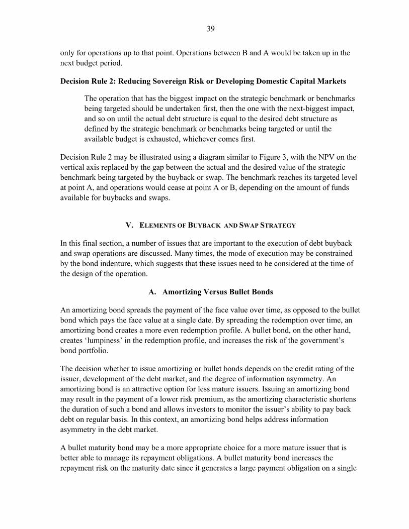
39

only for operations up to that point. Operations between B and A would be taken up in the next budget period.

Decision Rule 2: Reducing Sovereign Risk or Developing Domestic Capital Markets

The operation that has the biggest impact on the strategic benchmark or benchmarks being targeted should be undertaken first, then the one with the next-biggest impact, and so on until the actual debt structure is equal to the desired debt structure as defined by the strategic benchmark or benchmarks being targeted or until the available budget is exhausted, whichever comes first.

Decision Rule 2 may be illustrated using a diagram similar to Figure 3, with the NPV on the vertical axis replaced by the gap between the actual and the desired value of the strategic benchmark being targeted by the buyback or swap. The benchmark reaches its targeted level at point A, and operations would cease at point A or B, depending on the amount of funds available for buybacks and swaps.

V. ELEMENTS OF BUYBACK AND SWAP STRATEGY

In this final section, a number of issues that are important to the execution of debt buyback and swap operations are discussed. Many times, the mode of execution may be constrained by the bond indenture, which suggests that these issues need to be considered at the time of the design of the operation.

A. Amortizing Versus Bullet Bonds

An amortizing bond spreads the payment of the face value over time, as opposed to the bullet bond which pays the face value at a single date. By spreading the redemption over time, an amortizing bond creates a more even redemption profile. A bullet bond, on the other hand, creates ‘lumpiness’ in the redemption profile, and increases the risk of the government’s bond portfolio.

The decision whether to issue amortizing or bullet bonds depends on the credit rating of the issuer, development of the debt market, and the degree of information asymmetry. An amortizing bond is an attractive option for less mature issuers. Issuing an amortizing bond may result in the payment of a lower risk premium, as the amortizing characteristic shortens the duration of such a bond and allows investors to monitor the issuer’s ability to pay back debt on regular basis. In this context, an amortizing bond helps address information asymmetry in the debt market.

A bullet maturity bond may be a more appropriate choice for a more mature issuer that is better able to manage its repayment obligations. A bullet maturity bond increases the repayment risk on the maturity date since it generates a large payment obligation on a single

40

day, requiring the issuer to have enough liquidity or cash on this day. It is then not a surprising practice for debt managers to buy back at least a part of the outstanding bullet bonds ahead of the maturity date to smooth the need for cash at maturity. This may well require the issuer to engage in regular buyback operations, and the market to be sufficiently liquid to carry out these operations. Also, the debt market must be sufficiently well developed to provide the investors with other short or long-term instruments to minimize their reinvestment risk.

B. New Issues Versus Re-Opening Existing Issues

To raise funds in the bond market, an issuer needs to decide whether to issue a new bond or to re-open an existing issue. A new bond, particularly if designed as a bench market bond along the yield curve, facilitates price discovery. A re-opening involves issuing a debt instrument that is fungible with an already existing instrument, that is, identical in its characteristics such as maturity date or the coupon rate. Re-openings often aim at increasing the liquidity of existing or intended benchmark issues not only to facilitate price discovery, but also to enhance the functioning of the market for fixed-income or derivative instruments. Re-openings also help the issuers to avoid segmentation of the bond market and ‘overcrowding’ of the yield curve.

Bonds should be re-opened (or increased) soon after they are issued. Early re-openings allow the government to build a benchmark issue quickly, while spreading the number of times it accesses the markets. Similarly, quick re-openings help attract investors that purchase the initial issue, with the expectation that subsequent re-openings will raise the liquidity of the bond. Importantly, late re-openings may become difficult, if not impossible to carry out because of changes in interest rates or changes in the tax law or regulations. If the interest rates at the time of re-opening are much lower than the coupon rate of the initial bond, re-opened bonds will trade at premium, and may not be attractive to investors. Changes in tax law or regulations will imply different treatment of the old and new investors and may reduce the investors’ return on the new bond20, while substantial changes in interest rates will dramatically change the valuation of the re-opened bonds.

Re-opening of an existing bond issue has several disadvantages. First, a re-opening leads to lumping of debt service payments on one day, especially if the re-opened bond has a bullet maturity. Second, inappropriate timing increases the likelihood that the coupon will be out of

20 An example of such a change is the impact of the European Union savings directive or changes in the German tax law. To promote financial innovation and investments, the new law states that retail investors do not pay capital gains tax if they purchase bonds that trade within a certain limit below par. When the re-opened bonds are priced below this limit, they stop being attractive to the retail investors, and, effectively, are not fully fungible with the existing issue.

41

date and, therefore, the re-opened bonds will not attract investors. Finally, by re-opening an existing bond, the issuer forgoes the benefits of a new issue, such as the opportunity to create a new benchmark bond along the yield curve.

C. Call Options Versus Secondary Market Purchases

From the sovereign’s perspective, the exercise of a call option has definite advantages over the repurchase of a bond in the secondary market, particularly when the market price of a bond is higher than its face value (as discussed in Section IV.C). This suggests that governments that undertake debt buybacks and swaps on a regular basis should consider issuing bonds with embedded call options. It should be noted, however, that the inclusion of a call option would raise the cost of borrowing to the government since there is normally a call premium attached to these bonds. In other words, the government would have to compensate bondholders for the re-investment risk that a call option entails. In addition, call options are valuable for the sovereign if interest rates fall, since the bond can be refunded at a lower interest rate. When interest rates rise, however, the call option may not provide any benefit to the sovereign. Thus the benefits of a call option need to be carefully considered against the higher interest cost arising from the inclusion of the option.

D. Open Market Purchases Versus Open Tenders

An issuer may choose to repurchase or exchange bonds through either an open market transaction or a tender transaction. In an open market operation, the issuer buys back debt instruments at a price demanded by the seller or at the market price. In a tender offer, all sellers are treated equally and receive the same price. In defining the most appropriate mechanism to carry out these debt operations, the government needs to assess the characteristics of the secondary markets for external and domestic debt, while taking into account the size and timing of these operations. If the secondary bond market is sufficiently liquid, and market operations do not affect the price of debt instruments to a significant degree, then open market transactions may be cheaper than tender offers. All sellers receive their desired payments, which may help keep the total cost of the transaction lower than in the case of a tender offer, in which all investors receive the same payment for their bonds. However, in large buyback or swap programs, variable pricing and multiple transactions may result in higher costs and, thus, a uniform price and timing for all investors may be more cost efficient.

If secondary markets are liquid and well developed, the choice between open market purchases or open tenders would depend on practical considerations, such as simplicity, cost, and transparency. Depending on the circumstances, countries can engage in a secondary market accumulation (using cash reserves to buy back outstanding bonds directly in the secondary market), in a block trade exchange (simultaneously buying back old debt in the secondary market, and re-opening an existing bond issue to finance the buyback), or a public tender offer (public auction of new debt in exchange for selected old debt, including bonds or

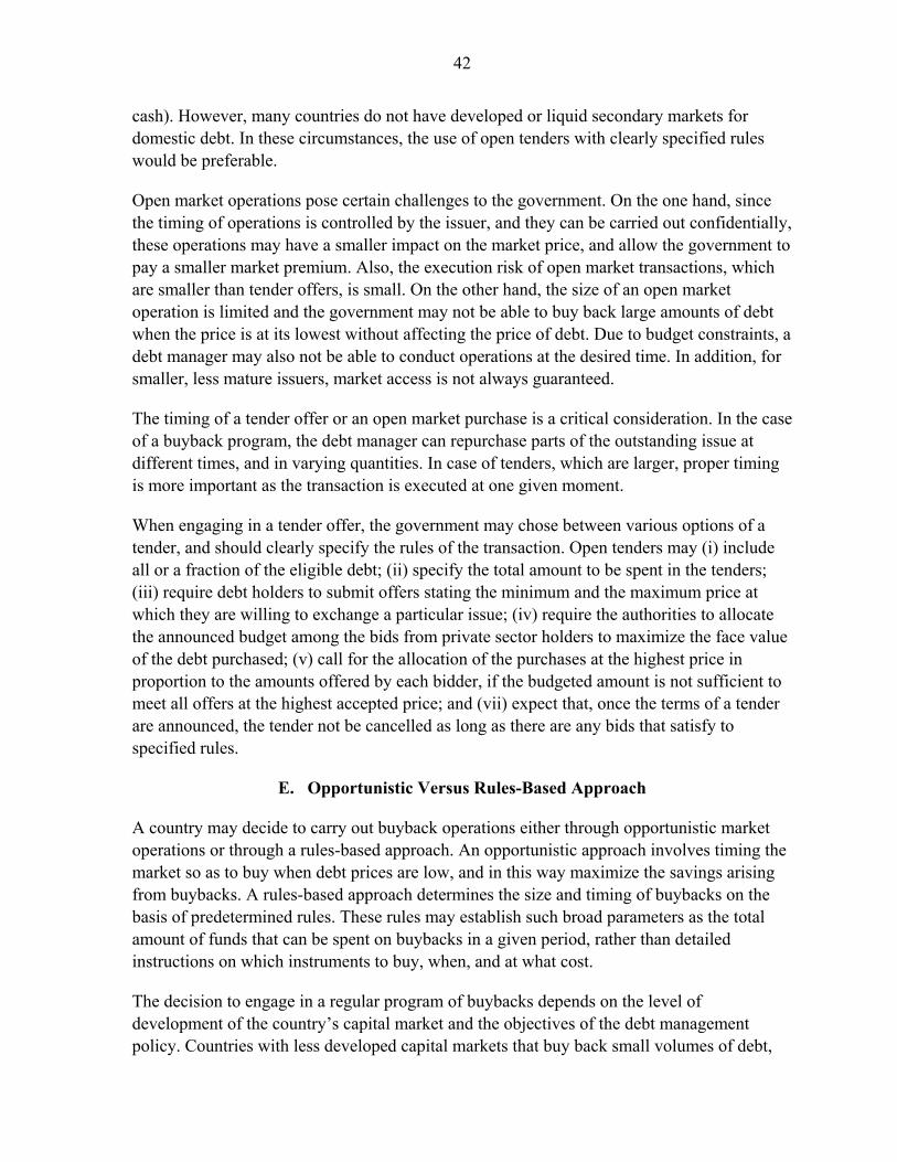
42

cash). However, many countries do not have developed or liquid secondary markets for domestic debt. In these circumstances, the use of open tenders with clearly specified rules would be preferable.

Open market operations pose certain challenges to the government. On the one hand, since the timing of operations is controlled by the issuer, and they can be carried out confidentially, these operations may have a smaller impact on the market price, and allow the government to pay a smaller market premium. Also, the execution risk of open market transactions, which are smaller than tender offers, is small. On the other hand, the size of an open market operation is limited and the government may not be able to buy back large amounts of debt when the price is at its lowest without affecting the price of debt. Due to budget constraints, a debt manager may also not be able to conduct operations at the desired time. In addition, for smaller, less mature issuers, market access is not always guaranteed.

The timing of a tender offer or an open market purchase is a critical consideration. In the case of a buyback program, the debt manager can repurchase parts of the outstanding issue at different times, and in varying quantities. In case of tenders, which are larger, proper timing is more important as the transaction is executed at one given moment.

When engaging in a tender offer, the government may chose between various options of a tender, and should clearly specify the rules of the transaction. Open tenders may (i) include all or a fraction of the eligible debt; (ii) specify the total amount to be spent in the tenders; (iii) require debt holders to submit offers stating the minimum and the maximum price at which they are willing to exchange a particular issue; (iv) require the authorities to allocate the announced budget among the bids from private sector holders to maximize the face value of the debt purchased; (v) call for the allocation of the purchases at the highest price in proportion to the amounts offered by each bidder, if the budgeted amount is not sufficient to meet all offers at the highest accepted price; and (vii) expect that, once the terms of a tender are announced, the tender not be cancelled as long as there are any bids that satisfy to specified rules.

E. Opportunistic Versus Rules-Based Approach

A country may decide to carry out buyback operations either through opportunistic market operations or through a rules-based approach. An opportunistic approach involves timing the market so as to buy when debt prices are low, and in this way maximize the savings arising from buybacks. A rules-based approach determines the size and timing of buybacks on the basis of predetermined rules. These rules may establish such broad parameters as the total amount of funds that can be spent on buybacks in a given period, rather than detailed instructions on which instruments to buy, when, and at what cost.

The decision to engage in a regular program of buybacks depends on the level of development of the country’s capital market and the objectives of the debt management policy. Countries with less developed capital markets that buy back small volumes of debt,

43

can undertake opportunistic operations on an ad-hoc basis, while timing them with favorable market conditions or income windfalls. Countries with more mature capital markets may use buybacks to manage liquidity, maintain an efficient yield curve and liquidity of benchmark issues, minimize the burden of large debt amortizations, or retire debt using an established source of financing, such as a special fund supported by oil or privatization revenues. In this case, a country may benefit from establishing a regular program of buybacks.

The choice between the opportunistic and a regular approach to debt buybacks is influenced by a number of practical concerns. The opportunistic strategy allows the country or the debt manager to conduct buyback operations when the debt market prices are low, while the rules-based approach limits the flexibility in the timing of operations. Temporary weakness of market prices makes it possible to retire larger amounts of debt using the same budget. The opportunistic approach can result in larger savings than the rules-based approach. However, detecting market weakness and proper timing of operations require sound knowledge of the market or specialized outside advice. The opportunistic approach can also lead to higher market volatility, as it makes investors uncertain about the timing and size of the operations. In this regard, a rules-based approach to buybacks can support market stability. Finally, the choice also depends on the liquidity in the secondary debt market and the ownership structure, especially concentration among creditors.

Regular buyback operations can negatively affect the cost of government borrowing. First, by increasing the demand for bonds and reducing their supply after a successful operation, buybacks may lead to an increase in bond prices. Second, a regular program of buybacks may lead to a permanent increase in risk premium demanded by investors, who want to be remunerated for higher reinvestment risk and administrative costs created by buybacks. To lower the reinvestment risk, it would be important for the local capital market to be well developed so that there are other instruments available to investors participating in a buyback.

An important element of a buyback program affecting its credibility and market stability is the source and amount of funds allocated to debt buybacks. To minimize uncertainty, the authorities should base the allocated amounts on actual flows. To avoid a conflict between the goals of a regular buyback program and short-term fiscal needs of the government or political pressures, the authorities could authorize aggregate spending over a specified period instead of approving individual debt buybacks. An effective way to finance and execute debt buybacks could be to establish an independent trust fund, financed by clearly defined sources of revenue, and managed by an independent board and a technical team. Such a set-up would increase the transparency of a buyback program, and minimize the number of intermediary steps between the financial inflow and a debt repurchase transaction. Alternatively, buybacks can be handled by a debt management office or agency, provided they are independent in executing the buyback program. The same body may also handle opportunistic debt buybacks.

44

F. Transparency and Investor Relations

Transparency and disclosure of information related to debt management enhance the credibility of the debt management strategy and help achieve its objectives by facilitating the execution of individual debt transactions. The authorities should clarify the objectives of the debt strategy and its placement within the wider macroeconomic framework. This can help reduce the uncertainty or asymmetric information on debt strategy within the wider financial community. The authorities should also communicate the division of responsibilities over debt management, rules and procedures of debt management operations, such as buybacks and swaps, and characteristics of debt instruments. This, in turn, may lower the transaction costs of investors or participants in debt management operations (such as investment banks), lead to a higher participation rate, and lower debt service costs. It is important that all participants in debt management operations understand and agree on the legal and administrative aspects of these operations (such as licensing of primary dealers and intermediaries, rules governing the secondary debt market, auction format and participation rules, and tax treatment of government debt instruments).

In the case of debt buybacks and swaps, the authorities need to communicate effectively with creditors and provide them with sufficient information related to these transactions. Such communication is essential to establish the credibility of debt buyback and swap programs. In this context, the authorities should, in particular, describe details of the buyback program at the beginning, and disclose the results of the program at the conclusion. To enhance accountability, they also need to regularly disclose the results of reviews and audits, and show the use of available funds. Finally, to increase support for the operations, the authorities should explain to the public the rationale for the buybacks and the workings of the process. For a successful debt swap, the authorities need to inform investors about the objectives of the swap, the amount of available funds, and the impact of the swap on the risk profile of the public debt. The authorities should also indicate how a given swap operation fits into the wider debt management strategy. In addition, to maximize the participation rate, the authorities should obtain and, if necessary, incorporate feedback from the investors in the design of a swap. To this end, meetings with creditors, for example during roadshows, are very beneficial.

45

Appendix 1. A Hypothetical Debt Swap Operation

A simple hypothetical example illustrates how a debt swap may be used to lower a bond’s debt service payments (see Appendix Table 1). In the example, an existing bond maturing in five years is exchanged for another bond with the same face value and also maturing in five years but with a lower coupon. The existing (old) bond, which may be callable or non-callable, has a face value of US$1 billion and a coupon of 10 percent (paid semi-annually), and a Macaulay duration of 4.12 years. The bond is trading at 112 percent of face value (US$1.125 billion), at a yield of 7 percent. The new bond, which is assumed to be non-callable, is issued at par at a coupon and yield of 7 percent—equal to the yield on the old bond. Because of the lower coupon, the new bond has a slightly higher Macaulay duration (4.3 years) than the old bond.

Two situations are examined below: where the old bond has a call option that is being exercised, and where the old bond is non-callable.

In the case of a callable bond:

The discounted value of the cash flows of the old bond ( oldV ), using the yield on the new bond (the opportunity cost of the swap) as the discount rate, is US$1.125 billion. This represents the savings (benefits) from the swap. The strike price is assumed to be 105 percent of the face value of the bond at the time of the swap, which means the re-purchase price (E) of the bond is US$1.05 billion. Total transactions costs of the swap (A) are assumed to be half of one percent of the sum of the face values of the two bonds (which is equal to US$10 million). The NPV of the swap is therefore US$65 million ( =−− AEVold US$1.125 million-US$1.050 million-US$10 million). This is the net benefit to the government from refinancing to take advantage of the decline in the interest rate.

In the case of a non-callable bond: The outcome here is different under the stipulated conditions. The discounted value of the cash flows of the old bond ( oldV ) and the transactions costs (A) remain unchanged, but the re-purchase price of the old bond (E) is different. It is assumed that all bondholders will only sell the bond if they are offered the market price, so that the re-purchase price of the non-callable bond is the market price. However, the market price is exactly equal to oldV , because the yield on the old bond (which is used to discount the cash flows to obtain the market price) is the same as that on the new bond. This means that EVold = , and therefore the NPV of the swap is minus US$10 million ( =−− AEVold US$1.125 million-US$1.125 million-US$10 million). For the NPV to be positive, the yield on the new bond would have to be lower than that on the old bond (the breakeven rate is just above 6.75 percent), or the re-purchase price of the old bond would have to be less than the market value by at least US$10 million (the required transfer of wealth from bondholders to the government to cover the transactions costs of the swap).

46

App

endi

x Ta

ble

1. Il

lust

ratio

n of

a H

ypot

hetic

al D

ebt S

wap

1-Ju

l-07

1-Ja

n-08

1-Ju

l-08

1-Ja

n-09

1-Ju

l-09

1-Ja

n-10

1-Ju

l-10

1-Ja

n-11

1-Ju

l-11

1-Ja

n-12

Term

of c

ash

flow

s (ye

ars)

0.5

11.

52

2.5

33.

54

4.5

5

Old

bon

d

Mat

urity

(yea

rs)

5

Fac

e va

lue

(US$

mill

ion)

1,00

0.00

M

arke

t val

ue (U

S$ m

illio

n)1/

1,12

4.75

C

oupo

n (p

erce

nt)

0.10

Y

ield

(per

cent

)0.

07

Cas

h flo

ws (

US$

mill

ion)

Prin

cipa

l1,

000.

00

I

nter

est

50.0

050

.00

50.0

050

.00

50.0

050

.00

50.0

050

.00

50.0

050

.00

D

isco

unt f

acto

rs 2

/1.

0350

1.07

121.

1087

1.14

751.

1877

1.22

931.

2723

1.31

681.

3629

1.41

06

Pre

sent

val

ue o

f cas

h flo

ws (

US$

mill

ion)

1,12

4.75

48.3

146

.68

45.1

043

.57

42.1

040

.68

39.3

037

.97

36.6

974

4.36

M

acau

lay

dura

tion

(yea

rs)

4.12

0.02

0.04

0.06

0.08

0.09

0.11

0.12

0.14

0.15

3.31

New

bon

d (n

on-c

alla

ble)

M

atur

ity (y

ears

)5

F

ace

valu

e (U

S$ m

illio

n)1,

000.

00

Mar

ket v

alue

(US$

mill

ion)

1,00

0.00

C

oupo

n (p

erce

nt)

0.07

0

Yie

ld (p

erce

nt)

0.07

0

Cas

h flo

ws (

US$

mill

ion)

Prin

cipa

l1,

000.

00

I

nter

est

35.0

035

.00

35.0

035

.00

35.0

035

.00

35.0

035

.00

35.0

035

.00

D

isco

unt f

acto

rs 2

/1.

0350

1.07

121.

1087

1.14

751.

1877

1.22

931.

2723

1.31

681.

3629

1.41

06

Pre

sent

val

ue o

f cas

h flo

ws (

US$

mill

ion)

1,00

0.00

33.8

232

.67

31.5

730

.50

29.4

728

.47

27.5

126

.58

25.6

873

3.73

M

acau

lay

dura

tion

(yea

rs)

4.30

0.02

0.03

0.05

0.06

0.07

0.09

0.10

0.11

0.12

3.67

Re-

purc

hase

pric

e of

old

bon

d (U

S$ m

illio

n)

Cal

labl

e bo

nd1,

050.

00

Non

-cal

labl

e bo

nd1,

124.

75

Tran

sact

ions

cos

ts (U

S$ m

illio

n)10

.00

NPV

of s

wap

(US$

mill

ion)

C

alla

ble

bond

64.7

5

Non

-cal

labl

e bo

nd-1

0.00

1/ F

or a

non

-cal

labl

e bo

nd. U

nder

lyin

g m

arke

t val

ue fo

r a c

alla

ble

bond

.2/

Dis

coun

t rat

e is

yie

ld o

n ne

w b

ond.

47

REFERENCES

Achraya, Sankarshan and Ishac Diwan, (1993). “Debt Buybacks Signal Sovereign Countries’ Creditworthiness: Theory and Tests,” International Economic Review, Vol. 34., No. 4: 795-817.

Aizenman, Joshua, Kenneth Kletzer, and Brian Pinto (2005). “Sargent-Wallace Meets Krugman-Flood-Garber, or: Why Sovereign Debt Swaps Do not Avert Macroeconomic Crises,” The Economic Journal, 115 (April): 345-367.

Ang, Andrew and Jun Liu (2004). “How to Discount Cashflows with Time-Varying Expected Returns”, The Journal of Finance, Vol. LIX, No. 6: 2745-2783.

Bowlin, Oswald (1966). “The Refunding Decision: Another Special Case in Capital Budgeting,” The Journal of Finance, Vol. 21, No. 1: 55-68.

Boyce, W. M. and A. J. Kalotay (1979). “Optimum Bond Calling and Refunding”, INTERFACES, Vol. 9, No. 5: 36-49.

Bulow, Jeremy and Kenneth Rogoff (1988). “The Buyback Boondoggle”, Brookings Papers on Economic Activity, Vol. 1988, No. 2: 675-704.

Bulow, Jeremy and Kenneth Rogoff (1991). “Sovereign Debt Repurchases: No Cure for Overhang,” The Quarterly Journal of Economics, Vol. 106, No. 4: 1219-1235.

Burgher, John and Francis Warnock (2006). “Local Currency Bond Markets,” IMF Staff Papers Vol. 53, Special Issue: 133-146.

Claessens, Stijn and Ishac Diwan (1989). “Market-Based Debt Reduction.” In Ishrat Husain and Ishac Diwan, eds., Dealing with the Debt Crisis. Washington D.C.: The World Bank.

Danmarks Nationalbank (2006). Danish Government Borrowing and Debt – 2005. http://www.nationalbanken.dk/C1256BE9004F6416/side/Danish_Government_Borrowing_and_Debt_2005!opendocument

Doodley, Michael P. (1989). “Buy-Backs, Debt-Equity Swaps, Asset Exchanges, and Market Prices of External Debt.” In Jacob A. Frenkel, Michael P. Dooley, and Peter Wickham, eds., Analytical Issues in Debt. Washington D.C.: International Monetary Fund.

Dornbusch, Rudiger and others (1988). Comments on Bulow and Rogoff’s paper. “The Buyback Boondoggle,” Brookings Papers on Economic Activity, Vol. 1988, No. 2: 675-704.

Fabozzi, Frank J. (2006). Fixed Income Mathematics: Analytical and Statistical Techniques, 4th ed. Mc-Graw Hill.

48

Finnerty, J. D. and D. R. Emery (2001). Debt Management. A Practitioner’s Guide. Cambridge, Massachusetts: Harvard University Press.

Hausmann, Ricardo and Ugo Panizza (2003). “The Determinants of Original Sin: An Empirical Investigation,” The Journal of International Money and Finance 22: 957-990.

IBRD (2000). Good Practice Notes, October 2000, Vol. 2-00.

International Monetary Fund (2003), Global Financial Stability Report. Washington, D.C., September.

International Monetary Fund and the World Bank (2003). Guidelines for Public Debt Management. Washington D.C.

Jorion, P. and Sarkis Joseph Khoury (1996). Financial Risk Management: Domestic and International Dimensions. Cambridge, Massachusetts: Blackwell Publications.

Krugman, Paul (1988). “Financing vs. Forgiving a Debt Overhang”, Journal of Development Economics 29: 253-268.

Krugman, Paul (1989). “Market-Based Debt Reduction Schemes.” In Jacob A. Frenkel, Michael P. Dooley, and Peter Wickham, eds., Analytical Issues in Debt. Washington D.C.: International Monetary Fund.

Larraín, Felipe and Andrés Velasco (1990). “Can Swaps Solve the Debt Crisis? Lessons from the Chilean Experience.” Princeton Studies in International Finance, No. 69.

Office of the Auditor General of Canada (2000). “Department of Finance - Managing Canada's Debt: Facing New Challenges.” Chapter 8 in “2000 Report of the Auditor General of Canada”. http://www.oag-bvg.gc.ca/domino/reports.nsf/html/0008ce.html

OECD (2005). Advances in Risk Management of Government Debt.

Papaioannou, Michael (2006). “A Primer for Risk Measurement of Bonded Debt from the Perspective of a Sovereign Debt Manager.” IMF Working Paper WP/06/195, Washington D.C.

“Report on Bond Exchanges and Debt Buy-Backs: A Survey of Practice by EU Debt Managers” (2001). http://ec.europa.eu/economy_finance/publications/efc/report5.pdf

Sachs, Jeffrey, Jeremy Bulow, and Kenneth Rogoff (1988). “Comprehensive Debt Retirement: The Bolivian Example,” Brookings Papers on Economic Activity, Vol. 1988, No. 2: 705-715.

49

Storkey, Ian (2001). “Sovereign Debt Management: A Risk Management Focus”, The Finance and Treasury Professional, May 2001: 7-10.

Thomas, Jonathan (1996). “Default Costs, Willingness to Pay and Sovereign Debt Buybacks,” mimeo.

Tuckman, Bruce (2002). Fixed-Income Securities: Tools for Today’s Markets, 2nd ed. Hoboken, New Jersey: John Wiley and Sons.

United States General Accounting Office (2001). “Debt Management. Insights and Tools From Selected Nations,” GAO 02-14, Washington D.C.

Wheeler, Graeme (2004). Sound Practice in Government Debt Management. Washington D.C.: The World Bank.

World Bank (1999). Second Sovereign Debt Management Forum. Washington D.C.