A Presentation by

KAUSHIKA G S

Under the guidance of Prof.C S P Ojha

HYDRAULICS ENGINEERING GROUP DEPARTMENT OF CIVIL ENGINEERING INDIAN INSTITUTE OF TECHNOLOGY

ROORKEE ROORKEE – 247 667, Uttarakhand, INDIA

Prior to presenting my work, I would like to acknowledge the help I received from the various senior researchers in this field.

I would like to acknowledge Dr. S K Jain for his help and guidance in the understanding the concepts of modelling.

I would express my humble gratitude to Dr. N Balaji from IIT Madras for patiently working to provise us with reliable data for soil and land use assessment.

I am grateful to my collegues and friends and professors for making the data easily accessible through the IIT Delhi server.

Acknowledgements are due to the GRBMP TEAM OF iit Rorrkee and other participant IITs for their co operation

Above all, I would acknowledge Prof. CSP Ojha without whose support and advice I would be unable to present this work.

ACKNOWLEDGEMENTS

The Ganges basin covers about one third of the Indian sub continent.

It has high slope in the upper stretch and causes a high velocity in flow.

Also, apart from the rainfall contribution, the glacial melt has a considerable impact in the addition to the flow to the river.

The SWAT model is applied to the upper Ganga catchment upto Haridwar and covers about 22580km2

The application of SWAT to a Himalayan sub basin to study the discharge characteristics including snow melt contribution is discussed here.

INTRODUCTION

The presentation is organized in the following sequence Study area Data and data processing SWAT run Results and discussion Snow modelling Conclusion

ORGANIZATION OF THE PRESENTATION

STUDY AREA

The area here is the initial stretch of the Ganga catchment.

The project is a part of the Ganga River Basin Management Plan carried out By the Govt.

Of INDIA in collaboration with 7 IIT’s

The Ganges is a glacier fed Himalayan river. This initial stretch is highly slopy and

mountainous terrain.

The basin has a wide variety of soil types .The areal extent is around 22580km2

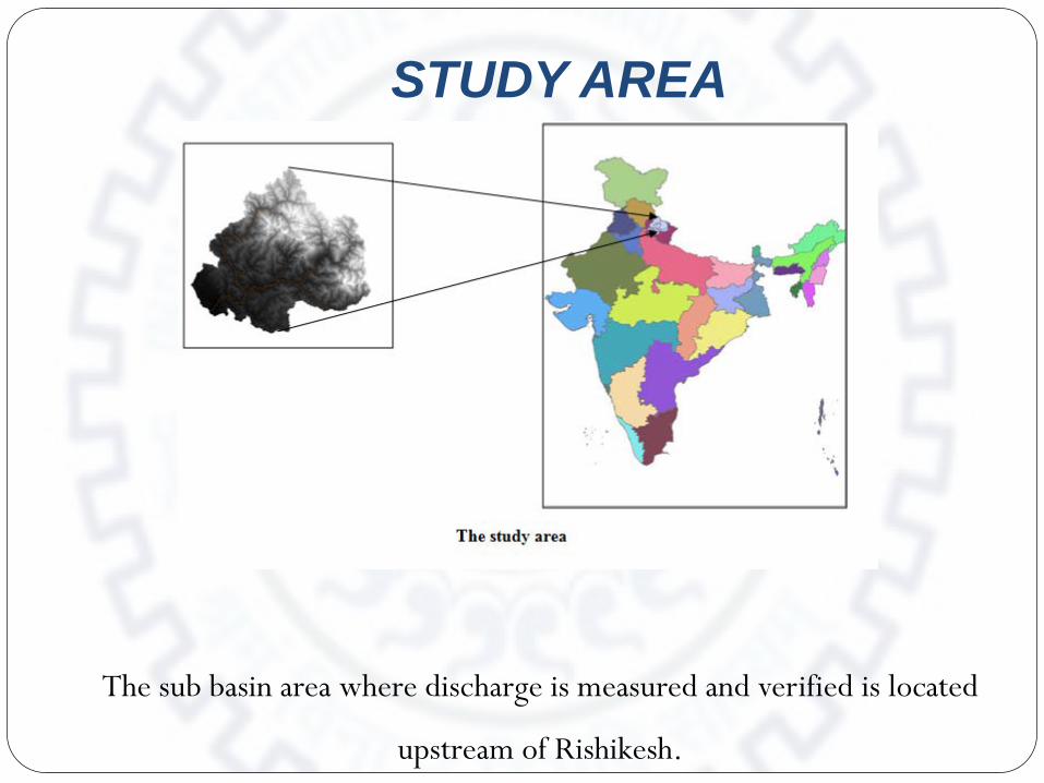
The sub basin area where discharge is measured and verified is located

upstream of Rishikesh.

STUDY AREA

DATA&DATA PROCESSING

Digital Elevation Model

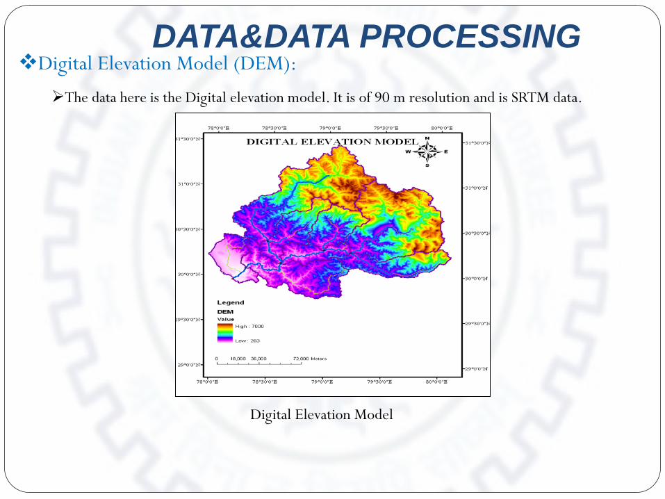
Digital Elevation Model (DEM):

The data here is the Digital elevation model. It is of 90 m resolution and is SRTM data.

DATA&DATA PROCESSING

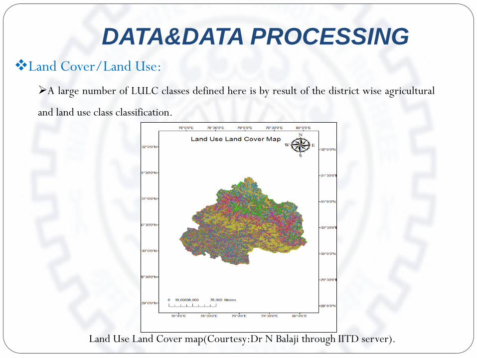
Land Use Land Cover map(Courtesy:Dr N Balaji through IITD server).

Land Cover/Land Use:

A large number of LULC classes defined here is by result of the district wise agricultural

and land use class classification.

DATA&DATA PROCESSING

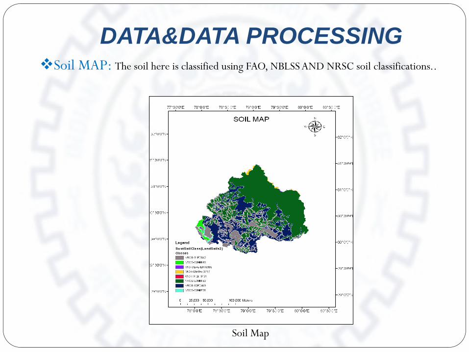
Soil MAP: The soil here is classified using FAO, NBLSS AND NRSC soil classifications..

Soil Map

DATA&DATA PROCESSING

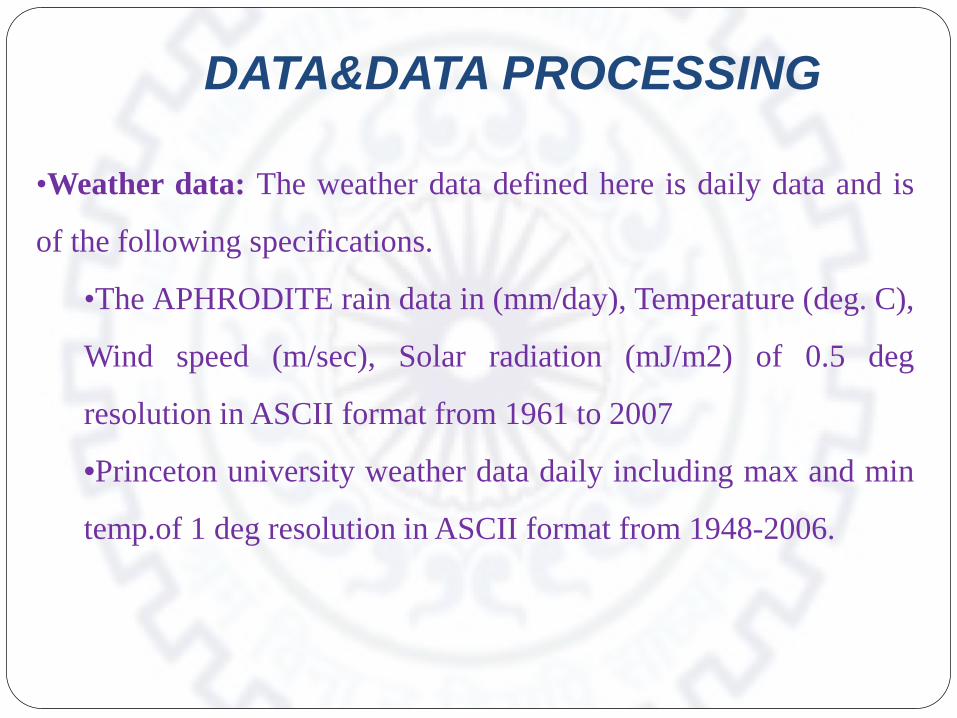
•Weather data: The weather data defined here is daily data and is

of the following specifications.

•The APHRODITE rain data in (mm/day), Temperature (deg. C),

Wind speed (m/sec), Solar radiation (mJ/m2) of 0.5 deg

resolution in ASCII format from 1961 to 2007

•Princeton university weather data daily including max and min

temp.of 1 deg resolution in ASCII format from 1948-2006.

SWAT RUN The SWAT model was run initially for a known period (1970-

1986) to check the validity of SWAT model for the basin.

The run was monthly and the outlet was selected based on

the location where the monthly data was recorded.

The flow was analysed for virgin condition assuming no

obstructions

RESULTS AND DISCUSSIONS

HRU analysis:

Area [ha] Watershed 2257965

Area [ha] %Wat.Area LANDUSE: forest-Evergreen --> FRSE 781216.7 34.6

Pasture --> PAST 527773.5 23.37 Range-Grasses --> RNGE 382910 16.96 SNOW --> SNOW 283187.7 12.54 Forest-Mixed --> FRST 215646.7 9.55 Rainfed --> A277 6478.722 0.29 Forest-Deciduous --> FRSD 60751.55 2.69

SOILS: NRCS-07N0163 1275603 56.49 NRCS-82P0469 590810 26.17 NRCS-91P0542 363506.1 16.1 NRCS-02N0640 28046.2 1.24

SLOPE: 50-80 757717.7 33.56 30-50 710308.3 31.46 0-30 578344.8 25.61 80-9999 211594.2 9.37

RESULTS AND DISCUSSIONS

The discharge here is corrected using a scaling factor ‘r’. The non snow analysis done here showed stimulations where there is considerable deficit between the observed and computed discharges. This can be seen in the plot shown. The preliminary analysis results are discussed here.the finetuning and further SWAT-CUP analysis is to be done as a future work.

RESULTS AND DISCUSSIONS

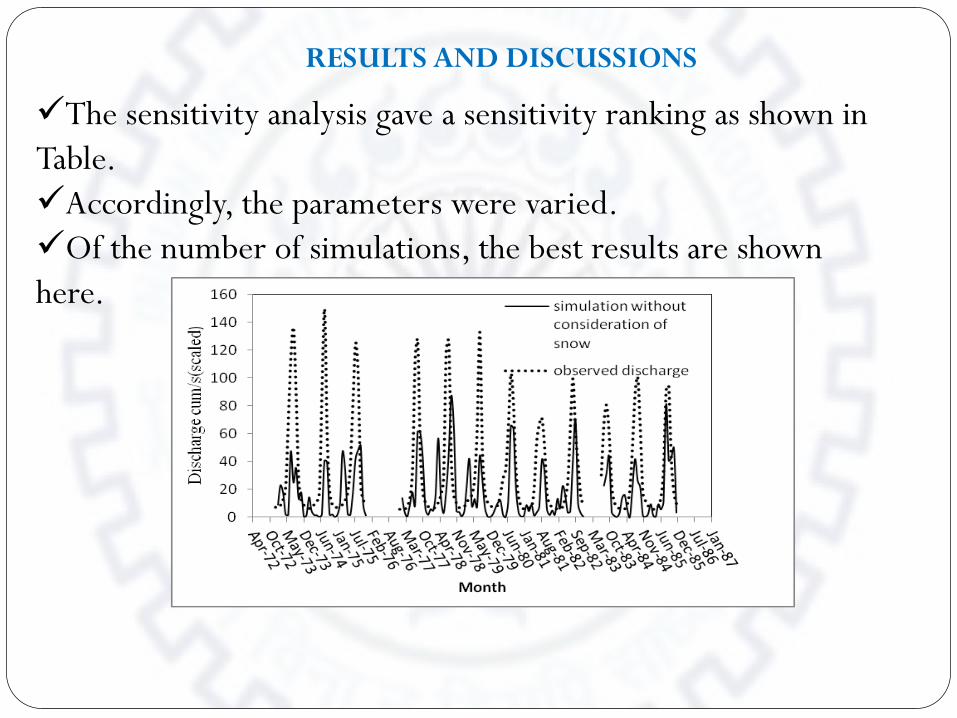
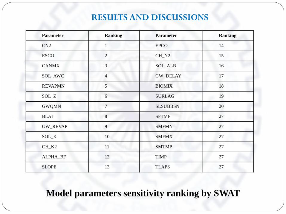
The sensitivity analysis gave a sensitivity ranking as shown in Table. Accordingly, the parameters were varied. Of the number of simulations, the best results are shown here.

Parameter Ranking Parameter Ranking

CN2 1 EPCO 14

ESCO 2 CH_N2 15

CANMX 3 SOL_ALB 16

SOL_AWC 4 GW_DELAY 17

REVAPMN 5 BIOMIX 18

SOL_Z 6 SURLAG 19

GWQMN 7 SLSUBBSN 20

BLAI 8 SFTMP 27

GW_REVAP 9 SMFMN 27

SOL_K 10 SMFMX 27

CH_K2 11 SMTMP 27

ALPHA_BF 12 TIMP 27

SLOPE 13 TLAPS 27

RESULTS AND DISCUSSIONS

Model parameters sensitivity ranking by SWAT

RESULTS AND DISCUSSIONS

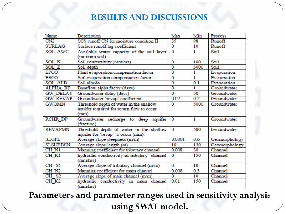
Parameters and parameter ranges used in sensitivity analysis using SWAT model.

SNOW MODELLING AND ANALYSIS The basin here has a major input from glaciers.

The basic snow model built in SWAT was redefined to model the

elevations and the corresponding snow depths available.

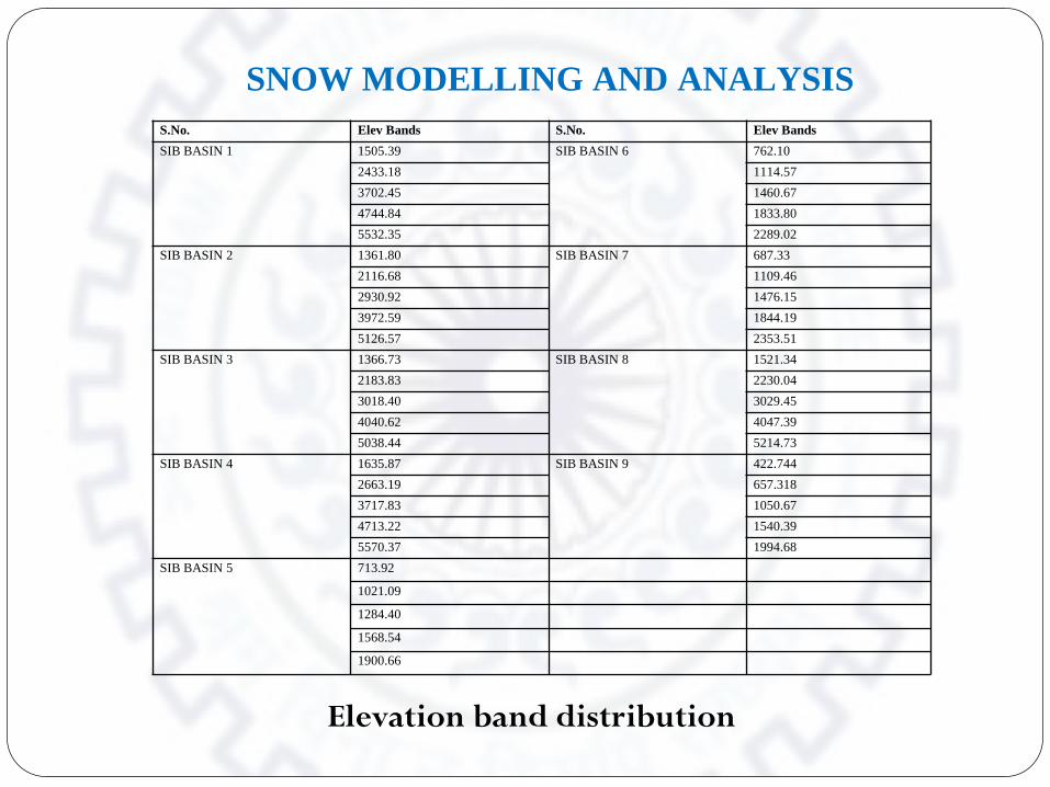
The snow melt contribution was analyzed by dividing the total

elevation into five elevation bands as in Table.

The snow depth initially considered to be zero was varied to about

3000mm from 300mm.

The model gave a very high discharge for snow depth of 3000 mm

indicating the dependency of the basin discharge to snowmelt

contribution.

S.No. Elev Bands S.No. Elev Bands SIB BASIN 1 1505.39 SIB BASIN 6 762.10

2433.18 1114.57 3702.45 1460.67 4744.84 1833.80 5532.35 2289.02

SIB BASIN 2 1361.80 SIB BASIN 7 687.33 2116.68 1109.46 2930.92 1476.15 3972.59 1844.19 5126.57 2353.51

SIB BASIN 3 1366.73 SIB BASIN 8 1521.34 2183.83 2230.04 3018.40 3029.45 4040.62 4047.39 5038.44 5214.73

SIB BASIN 4 1635.87 SIB BASIN 9 422.744 2663.19 657.318 3717.83 1050.67 4713.22 1540.39 5570.37 1994.68

SIB BASIN 5 713.92

1021.09

1284.40

1568.54

1900.66

Elevation band distribution

SNOW MODELLING AND ANALYSIS

SWAT over predicts the peaks in case of snow modelling and under-predicts the base flows (Fontaine et.al.,(2002)). Similarly, in this case, the peaks at four annual cycles are over predicted and the lows are under predicted.

SNOW MODELLING AND ANALYSIS

CONCLUSIONS SWAT applied to the upper Ganga catchment gives an idea of the vulnerability of the model to the terrain conditions and the discharge input variations. The variation of a number of vital parameters like the curve number or the base flow factor or even the ground water delay factor showed very less or no improvement in the model output. The sensitivity of the model to the snow melt contribution is ascertained here for this basin and the variation required in maintaining the authenticity of the model as applied to this basin is done here and is calibrated successfully. The error reduced to about 15% in the post calibration stage after snowmelt contribution was considered as compared to the 50% pre snowmelt calibration.