Embed Size (px)
Citation preview

A Predictive Model of Human Performance with
Scrolling and Hierarchical Lists
Andy Cockburn
University of Canterbury
Carl Gutwin
University of Saskatchewan
RUNNING HEAD: ANALYSIS OF SCROLLING AND
HIERARCHICAL LISTS
Corresponding Author’s Contact Information:
Associate Professor Andy Cockburn
Department of Computer Science
University of Canterbury
Christchurch
New Zealand
Brief Authors’ Biographies:
Andy Cockburn is a Computer Scientist with an interest in modelling and empirically measuring human performance with interactive systems; he is an Associate Professor in the Department of Computer Science of the University of Canterbury, Christchurch, New Zealand. Carl Gutwin is a Computer Scientist with interests in Computer Supported Cooperative Work and a wide range of issues within Human-Computer Interaction; he is a Professor in the Department of Computer Science of the University of Saskatchewan, Saskatoon, Canada.
ABSTRACT
Many interactive tasks in graphical user interfaces involve finding an item in a list, but with the item not currently in sight. The two main ways of bringing the item into view are scrolling of one-dimensional lists, and expansion of a level in a hierarchical list. Examples include selecting items in hierarchical menus and navigating through ‘tree’ browsers to find files, folders, commands, or email messages. System designers are often responsible for the structure and layout of these components, yet prior research provides conflicting results on how different structures and layouts affect user performance. For example, empirical research disagrees on whether the time to acquire targets in a scrolling list increases linearly or logarithmically with the length of the list; similarly, experiments have produced conflicting results for the comparative efficacy of ‘broad and shallow’ versus ‘narrow and deep’ hierarchical structures. In this paper we continue in the HCI tradition of bringing theory to the debate, demonstrating that prior results regarding scrolling and hierarchical navigation are theoretically predictable, and that the divergent results can be explained by the impact of the dataset’s organisation and the user’s familiarity with the dataset. We argue and demonstrate that when users can anticipate the location of items in the list, the time to acquire them is best modelled by functions that are logarithmic with list length, and that linear models arise when anticipation cannot be used. We then propose a formal model of item selection from hierarchical lists, which we validate by comparing its predictions with empirical data from prior studies and from our own. The model also accounts for the transition from novice to expert behaviour with different datasets.

CONTENTS
1. INTRODUCTION
2. RELATED WORK
2.1. Selection Performance in Scrolling and Hierarchical Lists
2.2. Performance Models for Interactive Systems
3. AN OVERVIEW AND MODEL OF THE TASK OF SELECTING FROM A LIST
4. VALIDATING THE SCROLLING MODELS
4.1. Apparatus
4.2. Procedure
4.3. Participants
4.4. Results
4.5. Discussion of the scrolling experiment
5. A MODEL OF HIERARCHICAL NAVIGATION
6. PREDICTIONS FOR BROAD/SHALLOW VS NARROW DEEP STRUCTURES
6.1. Predictions for the Miller/Kiger/Snowberry hierarchies
6.2. Predictions of the Landauer and Nachbar hierarchies
7. TESTING THE MODEL
7.1. Procedure
7.2. Apparatus
7.3. Participants
7.4. Results
8. GENERAL DISCUSSION AND CONCLUSIONS
8.1. Accuracy of the model
8.2. Generalising from lists to any spatial layout
8.3. How can the model be used by designers?
8.4. From empiricism to theory

1. INTRODUCTION
Most user interfaces provide access to more commands and to more data than can be conveniently displayed at once within the window. Scrolling and hierarchical organisation are two widely used techniques for allowing users to navigate through large command- and data-spaces. Figure 1 shows a variety of interfaces exemplifying these organisational strategies.
Designers face complex decisions in determining how best to combine scrolling and hierarchy to optimise performance. Their decisions are guided by factors such as consistency and semantics of the commands and data, but these factors do not answer performance questions. For example, would the cascading ‘Start’ menu shown in Figure 1a allow faster performance if flattened to a single scrolling list?; or could the flat list of fonts in Figure 1b be improved by grouping items into cascading menus based on initial letter or serif type?
Figure 1. Interfaces using some combination of hierarchy and scrolling to select
commands or data items.
(a) Cascading menus. (b) Font selection.
(c) EndNote commands. (d) Windows Explorer.

Prior research does not provide much guidance in making such choices. Empirical studies of scrolling, for example, differ on whether performance is best modelled by logarithmic (Hinckley, Cutrell, Bathiche and Muss 2002) or linear (Andersen 2005) functions of document length. There has also been research contention over whether hierarchical navigation is best supported through broad/shallow or narrow/deep hierarchies. For example, Miller (1981) examined the time taken to select one item from 64 choices in structures of varying depth and breadth, concluding that performance was optimal at medium depth. In replicating and elaborating Miller’s study, however, Snowberry et al. (1983) found fastest performance with a flat structure of 64 items that revealed four item categories, leading them to state that “our results suggest an advantage for broad structures”, (p. 704). Many others have replicated one set of findings or the other (reviewed below).
In this paper, we theoretically and empirically clarify the cause of these conflicting results, and we describe a model that predicts performance in tasks that involve selection of items from lists that use hierarchies, scrolling, or both. The most important aspect of the model is that it acknowledges the impact that data organisation has on performance. Section 2 reviews related empirical and theoretical work on interaction with scrolling and hierarchical lists. Sections 3 and 4 then present and validate models predicting item selection times in scrolling and non-scrolling lists. Section 5 extends the model to hierarchical item selection, and Section 6 compares the model’s predictions with empirical results from seminal studies. Section 7 reports the results of a study testing the model’s predictions in cases not covered in prior work, including the users’ transition from novice to expert performance. Sections 8 and 9 describe areas for further work and conclude.
2. RELATED WORK
Our work builds on two main areas of prior research: studies of performance in scrolling and hierarchical lists, and human performance models for interactive systems.
2.1. Selection Performance in Scrolling and Hierarchical Lists
The original motivation for our work was the conflicting results that have been reported about how humans perform with two related types of list widget: scrolling lists and hierarchical lists. We review the prior results for both types here.
2.1.1. Selection from Scrolling Lists
Scrolling list widgets present a small window onto a large one-dimensional dataset: the window shows only a portion of the data, and scrolling moves the data up or down behind the window. Scrolling has been widely studied in HCI (e.g., (Zhai, Smith and Selker 1997), (Hinckley et al. 2002), (Cockburn, Savage and Wallace 2005)), and has been reported as a potential performance bottleneck (e.g., (Byrne, John, Wehrle and Crow 1999), (O'Hara and Sellen 1997)). A wide variety of alternatives to the standard scroll bar have been proposed and evaluated, and we briefly review these below. We focus on techniques that provide direct control over the portion of the information space displayed

within the window, which intentionally excludes ‘Find’ or ‘Search’ utilities, which allow direct access to the contents of the list rather than to the space in which it is contained. Search utilities are independent of scroll-based view controls, since they can be assumed to be available regardless of the interface used to control scrolling (although they are rarely available in standard list widgets).
Scroll-based selection from a list can be viewed as a special case of target acquisition, where the target is initially outside the viewable region. Removing the constraint of initial target visibility has a dramatic impact on user interaction, and as a result designers have developed a wide range of scrolling techniques. Commercial graphical user interfaces provide a very wide range of widgets for scrolling, including scrollbars, paging controls, and rate-based scrolling (Zhai et al. 1997) (activated with the middle mouse button). Input devices such as keypads, mouse scroll-wheels, and other buttons also allow direct control over the view.
Despite its ubiquity there is research contention over how empirical measures of scrolling performance match theoretical models. Hinckley et al (2002) used a bi-directional tapping task, where users repeatedly scrolled to two targets in a document, to show that scroll-based target acquisition is modelled by Fitts’ Law (Section 2.2). Although the resulting throughput values were low (approximately 1bit/sec) compared to traditional on-screen pointing (typically above 5bits/sec), the Fitts’ models were strong (R2 in the range 0.81 to 0.95) for several types of scroll control (isometric input rate-control with the IBM ScrollPoint Pro mouse, two acceleration functions with the Microsoft IntelliMouse scroll wheel, and a standard scroll wheel).
In a more recent study, however, Andersen (2005) disagrees with Hinckley’s results, claiming that empirical data from a task that ‘more closely resembles scrolling’ (p. 1183) the data shows a strong linear fit with scroll distance (R2=0.97) rather than the logarithmic one anticipated by Fitts’ Law. Andersen’s tasks involved visually searching through a document to find a target line that was highlighted with a red background.
2.1.2. Hierarchical navigation
As with scrolling, there has been extensive research into the comparative efficiency of navigating through different types of hierarchical structures, particularly comparing deep structures containing few items at each level with shallow structures containing many.
Miller’s (1981) early study compared hierarchical menu performance times in accessing one of 64 leaf nodes in structures that varied depth from one to six levels, with between two and 64 items in each level: 26 (two item at each of six levels of depth), 43, 82 and 641. Plotting the acquisition time results against number of choices per level revealed a U-shaped curve, with best performance in the 82 condition. Items were randomly ordered within each level of the hierarchies used.
Snowberry, Parkinson and Sisson (1983) replicated Miller’s experiment, adding one condition and a pre-screening process. The additional condition, called CAT64, used four stable categorized item groups within a 641 structure (rather than Miller’s random-only

ordering). They also pre-screened participants for memory and visual-scanning capability. Results of the replicated conditions supported those of Miller, but the CAT64 condition yielded the fastest access of all. They state “when categorical grouping was maintained across hierarchies our results suggest an advantage for broad structures” (p. 704). Furthermore, Snowberry et al. showed that CAT64 allowed the largest performance improvement between blocks of trials. Finally, they showed that pre-screened measures of the participants’ visual scanning capability predicted user performance, while memory measures did not.
Snowberry et al.’s results are important to our model and studies. They show that certain types of data organisation yield different performance characteristics, both in acquisition time and in transition to expert performance; in other words, the data type influences the efficiency of depth/breadth considerations in hierarchical structure. To our knowledge this result has not been explicitly pursued in subsequent research. Instead, many researchers have continued to study the general question of whether structures should be deep or broad (briefly reviewed below). We contend, and demonstrate in this paper, that this general question is unanswerable, since it depends on the contents of the menu and on how long users are expected to interact with it.
Kiger (1984) also examined navigation to 64 leaf items, using five different structures: 26, 43, 82, 4×16 and 16×4. Items were randomly ordered at each level of the hierarchy, and experience-based performance changes were not examined. Results showed that performance degraded with depth, and that performance was similar for the three conditions with two-level structures. Subjective measures favoured the 82 condition.
Jacko and Salvendy (1996) broke away from the prior work which examined different structures of 64 items. Instead, they examined performance, error rates and subjective preferences in six different structures containing between 4 (22) and 262144 (86) items. Exact details of the ordering of data within each level is not provided, but as the structures were reportedly “slight variations of the menus that had been used by both Miller (1981) and Kiger (1984)” (p1192), we assume that the order was random. Results showed that access times increased with depth and breadth, which they attributed to the associated increase in task complexity and associated affect on the user’s short-term memory.
Larson and Czerwinski (1998) examined navigation to one of 512 leaf items across three structures: 16×32, 32×16, and 83. Items within each level of the hierarchy were alphabetically sorted. Mean acquisition times were fastest in the 16×32 condition, although not significantly different from 32×16. The deep 83 structure was significantly slower than the other two conditions. Analysis of subjective measures showed split preferences across the three structures, but an analysis of “lostness” (deviation from the optimal path) suggested optimal performance in the 16×32 condition. These results lead Larson and Czerwinski to caution against excessively broad structures, arguing that narrower structures improve performance through a reduction in categorical decisions that users must make.

Zaphiris, Shneiderman and Norman (2002) compare performance with two alternative interfaces for hierarchical navigation on the web—‘expandable indices’ (folding-out new levels of detail in a manner similar to Microsoft Windows Explorer), and ‘sequential menus’, which simply replace the old level view with the new one. Like most previous studies, their results suggest that shallow structures improve performance (regardless of interface type), and that the sequential menu interface outperformed expandable indices.
Landauer and Nachbar’s study (1985) is the most similar prior work to our current study. As well as examining acquisition times to one of 4096 items in various breadth/depth configurations (212, 46, 84 and 163), they also proposed a performance model based on the sum of Hick-Hyman decision time and Fitts’ pointing time. Their model assumed the same branching factor and organisation scheme at all levels of the hierarchy.
Landauer and Nachbar’s empirical studies used hierarchies that were alphabetically or numerically ordered at all levels. Participants used a touch-sensitive screen to select between the n branching alternatives at that level of the hierarchy. Words were randomly selected from an on-line dictionary, and were between 4 and 14 characters in length. Numbers were between 1 and 4096.
Results showed performance advantages for broad/shallow structures. They report that selection time at each level was well modeled by T=a+b×logC, where C is the number of choices, in agreement with the series model of Hick-Hyman choice and Fitts’ pointing. They also provide an enlightening discussion of the conditions under which deeper and broader structures may profit (p77). To our knowledge this discussion has not been pursued.
Twenty-five years after Miller’s study, the question of “shallow-broad or deep-narrow” is still being tackled by researchers through empirical methods (e.g. Geven, Sefelin and Tscheligi’s (2006) recent study of depth versus breadth in mobile interfaces).
2.2. Performance Models for Interactive Systems
In addition to these specific studies that have investigated particular structures, several researchers have proposed and tested more general models that can predict human performance with interactive systems. We review some of these models below, including low-level psychomotor models such as Fitts’ Law and the Hick-Hyman Law, medium-level models such as the Keystroke-Level Model, and higher-level models such as GOMS that also consider cognitive processes.
2.2.1. A model of target acquisition: Fitts’ Law
Heavily researched in HCI, Fitts’ Law (1954) predicts the time taken to move to an item using a pointing device or finger: movement time MT=a+b×ID, where a and b are constants empirically determined through regression analysis. ID represents the ‘index of difficulty’ of the task (measured in bits), with ID=log2(A/W+1), where A and W represent the amplitude of movement and the width of the target. The reciprocal of the slope

constant b provides an estimation of the ‘throughput’ (measured in bits/sec) of a particular input device, representing the efficiency of the device in transferring human intentions to actions.
The relationship between movement time and target-distance/width is logarithmic rather than linear because human pointing to visual targets allows a large proportion of the distance toward the target to be rapidly completed without attending to feedback In control-theory and in human physiology research the terms ‘open-loop’ and ‘ballistic action’ are used to describe such processes, which are completed independent of sensory information. A closed-loop (feedback dependent) phase of motion follows the open-loop phase, allowing corrective actions that complete target acquisition. Figure 2 depicts the cursor velocity against time during a typical target acquisition process.
Figure 2. Cursor velocity during target acquisition. An initial high velocity open-
loop, or ‘ballistic’, phase of motion is followed by several closed-loop
corrective actions in the final stages of acquisition.
T im e
Cu
rso
r ve
locity
O pen-loop
im pulse
C losed-loop
corrective action
T im e
Cu
rso
r ve
locity
O pen-loop
im pulse
C losed-loop
corrective action
We will return to the user’s ability to exploit open-loop processing as an explanation of performance differences for different types of scrolling activities.
2.2.2. A model of choice selection: Hick-Hyman law
The Hick-Hyman Law (Hick 1952; Hyman 1953) models choice reaction time. Although much less widely used in HCI than Fitts’ Law (Seow 2005), both laws stem from the same information theoretic foundation (Shannon and Weaver 1949). The Hick-Hyman Law states that the time T to choose an item, when optimally prepared, is a linear relationship with the item’s information entropy H: T=a+b×H, where a and b are empirically derived constants, and H=log2(1/p), where p is the probability of the item appearing as the stimulus. Likely events have low information entropy, unlikely ones, high. When the user chooses between C equally probable alternatives, the Hick-Hyman Law can be re-written as T=a+b×log2(C).
2.2.3. Keystroke Level Model (KLM)
Card, Moran and Newell’s (1983) Keystroke Level Model (KLM) of task execution allows designers to predict the time experts take to carry out low-level actions with an

interface. KLM views tasks as consisting of a set of actions completed in series: Texecute=Tk+Tp+Th+Td+Tm+Tr, where k, p, h, d, m, and r represent the keyboard, pointing, homing, drawing, mental preparation and system response. Tm accounts for the time to retrieve skilled actions from memory, which Card, Moran and Newell state “are assumed to take an average of 1.35s each”. They provide heuristics to help designers determine when mental preparation operations need be inserted into a model. Tools automating much of the modelling process have also been developed (John, Prevas, Salvucci and Koedinger 2004).
Pointing (Tp) and mental preparation (Tm) times are of specific interest in this paper. Fitts’ law models for the acquisition of on-screen targets are well understood (Section 2.2.1), but pointing to off-screen targets through scrolling is less so (Section 2.1.1). The mental preparation component has also been the subject of research debate. Lane, Napier, Batsell and Naman (1993), for example, investigate whether hierarchical menu navigation using keyboard shortcuts (specifically, keystrokes W, I, and R for ‘worksheet’, ‘insert’, ‘row’) involve three separate Tm actions or one composite one; with results suggesting the latter.
Recently we proposed a menu performance model that provides a finer grained decomposition of the Tm operator, and which accounts for the transition from novice to expert performance (Cockburn, Gutwin and Greenberg 2007). The ‘Search/Decision+Pointing’ (SDP) model predicts that novice users visually search for menu targets causing search times to increase linearly with menu length. Experts, however, decide upon item location, and decision times are predicted by the Hick-Hyman Law (Section 2.2.2) to increase logarithmically with the number of equally probable items. Empirical performance data from a variety of menu designs matched the SDP model’s predictions extremely well.
Performance models for scrolling and hierarchy remain under-explored. Although our SDP model proposed an extension for cascading menus we did not evaluate it. The objective this paper, then, is to generalise the SDP model to cases where the user needs to select a series of targets, possibly with scrolling at each level, to reach an ultimate target within a hierarchy.
As well as low level performance models, there are many extensive cognitive modelling architectures available for HCI, most stemming from Card et al.’s seminal work on GOMS (Card et al. 1983). The primary disadvantage of using cognitive architectures for performance modelling is their substantial complexity, which puts them beyond the reach of most interface developers (Vera, John, Remington, Matessa and Freed 2005).
Our goal in the model presented below is to provide designers with a simple tool that can be used quickly and widely, with no more expertise than the designer’s intuitions about how the task will work, and the computational capabilities of a standard spreadsheet application.

3. AN OVERVIEW AND MODEL OF THE TASK OF SELECTING
FROM A LIST
In order to clarify and ground the model that follows, we here set out the actions and decisions that occur in the task of selecting an item from a scrolling or hierarchical list.
The user’s general task is to manipulate the controls of the list widget to bring the desired item into view, and then select the item with a pointing device. Assuming that the list is already visible in the interface, the following steps occur from the user’s perspective:
1. Determine where the desired item is likely to be, relative to the current location in the list
2. Determine what navigation action to take next, and carry out that action
3. If the desired item is still not visible, go to #1
4. If visible, move the cursor to the item and select
Step one is demanding as it involves comparing the target item with those in the display, and determining an appropriate direction and distance for subsequent movement. The user’s success in step one has a large effect on the number of times that the first two steps must be repeated.
For the user to be successful at determining where the desired item lies relative to their current position, they must have a mental model of the contents of the list. Although different users may have different mental models, there are clear characteristics of the list contents and of the user’s previous experience with it that influence how effectively they can exploit their model. These factors can be reduced to the basic idea of ‘how well the user knows the data.’ If the user knows the data well, either through experience or because the data is organized in a standard fashion (such as alphabetic ordering), then they will be able to rapidly move in the direction of the desired item. In terms of Fitts’ Law (Section 2.2.1), they will be able to use a ballistic impulse to bring the desired item into view. If, however, the user does not know the data well (e.g., the data is random, or its organizing principle is not yet known), then they must fall back on visual search, and inspect each item in turn in order to find the desired item.
The difference between known and unknown data has not been adequately addressed in prior empirical studies of selection from either scrolling or hierarchical lists. This factor plays a major role in the model described below – it allows us to predict selection performance as a range of behaviours between linear and logarithmic, and also provides a mechanism for explaining the user’s transition from one extreme to the other.
We argue that designers can predict whether performance will be linear or logarithmic with distance, depending on whether users can navigate toward the target using a feedback-free (open-loop) ballistic impulse, such as that illustrated in Figure 2. If

they can, then performance will be logarithmic with distance, and if not, it will be linear. For example, when searching an alphabetically sorted list for the word “trek”, the user can rapidly scroll through most of the alphabet before attending to the list contents. Similarly, if the user has extensive knowledge of location of items in the dataset through prior experience, then they can directly scroll to the vicinity of the item before browsing the items displayed.
The general form of the logarithmic model is given in Equation 1.
)1(log2 +×+= nbaM typetype Eq 1.
In this equation, constants atype and btype are empirically determined through regression analysis for a particular type of scrolling task, and n is a measure of the target distance. To calibrate a particular model, n could be the actual distance to a series of targets within a list of fixed length, or it could measure the list length for targets evenly distributed through lists of differing lengths. Example tasks enabling a ballistic impulse include searching for a known target in data that is sorted (alphabetically, numerically, temporally, etc.), and locating a target that resides at a known location within the list.
When the user must compare each item with the intended target (closed-loop processing) then acquisition time will increase linearly with distance, as given by Equation 2.
nbaM typetype ×+= Eq 2.
The following section validates this model of list selection tasks, and later sections generalise the model to hierarchical lists.
4. VALIDATING THE SCROLLING MODELS
We conducted an experiment to validate the hypothesis that list selection performance follows a linear model when the user’s task is dominated by visual inspection, and that logarithmic models arise with predictable data sets. We also use the data to calibrate the parameters atype and btype for different data arrangements, which will be reused in predictions later in the paper. Tasks in the experiment involved selecting a target word from lists of between 10 and 1280 five-letter words or word-ranges organized in one of three ways: randomly, alphabetically, or with the target location clearly demarked. The random condition represents a dataset that can only be searched with visual inspection, and hence selection time should increase linearly with the number of items. The alphabetic ordering and the clearly demarked conditions both allow the user to anticipate item location, and hence both should allow selection times that increase logarithmically with list length, but with different values for parameters atype and btype.
Figure 3 shows the experimental interface in two different conditions. The target item is displayed to the right of the “Go” button. In Figure 3a the user is seeking the target ‘lobed’ using the alphabetic word-range condition with 64 items – the user must click on the word range that contains the target (‘lined—loyal’ in this case). In Figure 3b the user

is seeking the word ‘below’ from 1280 items in the ‘flagged’ condition, which depicts the target’s location with a mark alongside the final scroll-thumb position, and by flagging and highlighting the target item in the list.
Figure 3. The list interface used in the calibration experiment.
(a) Alphabetic word-range condition
with 64 items.
(b) The ‘flagged’ condition with 1280
items
4.1. Apparatus
The experiment ran on a Compaq nx9010 laptop computer with a 15inch 1400x1050 resolution display. Input was received via an optical wireless mouse.
Software controlled the participants’ exposure to conditions and logged all user actions to millisecond granularity. The user interface was written in Tcl/Tk and ran in a window of 610×870pixels. The scrolling window of words displayed 40 lines of text. The list of 7560 five-letter words was retrieved from: www.math.toronto.edu/ jjchew/scrabble/lists/common-5.html
4.2. Procedure
All participants completed a series of word selections in six experimental conditions: Fitts, random-word, alphabetical-word, spatial, random-range, and alphabetical-range.
The first condition (‘Fitts’) was used to calibrate traditional Fitts’ Law pointing parameters. Tasks involved selecting a clearly demarked target word from a list of 40 five letter words, with no scrolling necessary. When the participant clicked the “Go” button the target word was displayed alongside the button, and a randomly selected list of 40

words appeared, with the target word highlighted red. Participants were instructed to carefully visually identify the target before moving to acquire it. Task time was taken from the instant the cursor left the “Go” button. Participants completed 25 selections; five at each of the 1st, 5th, 10th, 20th, and 40th position in the list. Data from the first five selections were discarded as training tasks.
The second condition (‘random-word’) was used to inspect performance in finding a target word within randomly ordered word lists of varying lengths. Within the list, the target was displayed identically to all other items without any highlighting. The hypothesis is that performance deteriorates linearly with list length. When the participant clicked the “Go” button, the target word was shown immediately right of the button, and a randomly selected set of words containing the target was displayed. Participants made twelve selections with a list of length ten (data from the first four discarded as training tasks), then eight each at lengths 20 and 40; they then made twelve selections at length 80 (data from the first four discarded as training tasks because these are the first tasks involving scrolling), then eight each at lengths 160 and 320 items. To control the difficulty of tasks at each length, each set of four selections contained one at each of 20, 40, 60 and 80% of the distance through the list (in a random order). Participants were not informed of this experimental control, and it is unlikely that any noticed it because the lists continually varied in length. Participants were instructed that the best way to solve the task was to carefully scan the list from the top to bottom, trying to be sure not to overshoot the target; they were told that they could scroll either using the scroll wheel or by using the scrollbar. They were also instructed to take a break between tasks if necessary, and they were required to take a brief break to advance after each block of eight or twelve tasks for a particular list length.
The third condition (‘alphabetical-word’) was used to inspect performance in selecting a target word from alphabetically ordered word lists of varying lengths. The hypothesis here is that selection time increases logarithmically with list length. The tasks were cued identically to the ‘random’ condition, with the only differences being that the list of words was alphabetically sorted and that a more extensive set of word lists was used: 10, 20, 40, 80, 160, 320, 640 and 1280 items. Like the ‘random’ condition, the blocks at length 10 and 80 contained twelve tasks, with data from the first four in each being discarded. All other blocks contained eight tasks, two at each of the locations 20, 40, 60 and 80% through the list.
The fourth condition (‘spatial’) was used to inspect optimal scroll-based off-screen target acquisition; trying to emulate performance when the user has a very strong spatial understanding of the location of their target in a scrolling list. The hypothesis (supported by Hinckley et al. (2002)) is that selection time increases logarithmically with list length. In this condition, the target was highlighted within the list in three ways. First, the location of the target within the scrollbar was depicted by a red marker alongside the scroll-thumb. Second, the target word was highlighted in red; and third, a small flag icon was placed to the left of the word. In this condition, the non-scrolling list lengths are theoretically identical to traditional Fitts’ Law pointing tasks, so only list lengths 80, 160, 320, 640 and 1280 items were evaluated, in that order. Again, all blocks consisted of

eight selections (two at each location 20, 40, 60 and 80% through the list), except for the first length, which had an additional four selections for training.
The fifth condition (‘random-range’) was used to calibrate performance in selecting a target alphabetical range that encloses a specific target word. The interface and task cueing were identical to the ‘random-word’ condition, except each item in the list displayed a unique alphabetical range such as ‘aback–bests’. The set of items in the list covered the entire range of the alphabet, but the ranges were randomly ordered. Participants were required to select the alphabetical range containing the target word: for example, ‘gawks–lidos’ for the target ‘gliff’. They completed a practice block of five selections, then six blocks of five selections at each length of 2, 4, 8, 16, 32, 64 items (order counterbalanced).
The sixth condition (‘alphabetical-range’) was identical to the random-range task, except the items in the list were in alphabetical order, as depicted in Figure 3a.
4.3. Participants
The nine participants (one female) were Computer Science post-graduate students and staff. All had at least six years experience with graphical user interfaces, and used computers as a primary function of their everyday work (more than 30 hours of use per week). They volunteered to participate in response to an email message to staff and students. They received no reward for participation.
4.4. Results
4.4.1. Fitts’ Law Tasks
As anticipated, data from the Fitts’ condition strongly adhered to the Fitts’ Law model, with regression analysis producing a best-fit model of MT=0.24+0.13×ID, R
2=0.96.
4.4.2. Acquisition of random words & word-ranges—linear with number of items
Data from the random conditions showed strong linear relationships between the length of the list and acquisition time.
For the list of individual words, regression analysis of acquisition time against number of list items gives a best fit model of T=-1.4+0.19×items, R
2>0.99, see Figure 4.
Further analysis shows that the best-fit models are similar whether scrolling was required (items=80, 160, 320) or not (items=10, 20 & 40):
No scroll, R2>0.99: T=0.43+0.12×items Eq 3.
Scroll, R2>0.99: T=-2.4+0.19×items Eq 4.

Figure 4. Results of the random word and word-range conditions.
Scrolling words T = - 2.4+0.19xitems
R 2 = 0.99
Non-scrolling words T= 0.43+0.12xitems, R 2 = 0.99
Word-ranges
T= 1.45+0.29xitems
R2= 0.99
0
10
20
30
40
50
60
70
0 50 100 150 200 250 300 350
Number of items
Me
an
se
lec
tio
n t
ime
(s
ec
s)
Non-scrolling words
Scrolling words
Word-ranges
The similarity of models for scrolling and non-scrolling conditions suggests that the human factors of visual search are the primary limitation of acquisition in random lists, not the interface mechanics of scrolling.
Data from the random word-range tasks (Figure 4) also conformed to a linear model, but with higher intercept and slope values than the individual words, as anticipated due to the more difficult task:
R2>0.99: T=1.45+0.29×items Eq 5.
4.4.3. Acquisition of sorted words and word-ranges—logarithmic with number of
items
Data from the alphabetical conditions strongly supported the model’s premise that acquisition times increase logarithmically with the number of items when the data is sorted (see Figure 5). For the word lists, regression analysis of the mean time for each length against number of items in the list gives a best fit model of T=-
2.6+0.97×log2(items+1), R2=0.96. Separating the analysis of list lengths that did not
require scrolling (lengths 10, 20, 40) from those that did (lengths 80, 160, 320, 640, 1280) shows markedly different models for the two conditions, but with extremely good fits in both cases, as follows:
No scroll, R2>0.99: T=-0.17+0.44×log2(items+1) Eq 6.
Scroll, R2=0.99: T=-5.13+1.28×log2(items+1) Eq 7.
Data from the word-range tasks (Figure 5) also conformed to the logarithmic model:
R2=0.99: T=-0.06+0.86×log2(items+1) Eq 8.

Figure 5. Results of the alphabetical word and word-range conditions.
Non-scrolling words
T= - 0.17+0.44xlog 2(items+1)
R 2= 0.99
Scrolling words
T = - 5.13+1.28xlog 2(items+1)
R 2= 0.99
Word-ranges
T = - 0.06+0.86xlog 2(items+1)
R 2= 0.97
0
1
2
3
4
5
6
7
8
9
0 2 4 6 8 10 12
Log2(items+1)
Me
an
se
lec
tio
n t
ime
(s
ec
s)
Non-scrolling words
Scrolling words
Word-ranges
4.4.4. Acquisition of spatial items—logarithmic with number of items
Data from the Fitts’ condition models spatial acquisition times for visible targets, where scrolling is not required. Data from the ‘spatial’ condition, where targets were flagged both in the scrollbar and on the target itself, represents ‘optimal’ scroll-based acquisition, where the user has a strong memory for the location of the item.
Regression analysis of the mean time for each length against number of items (80, 160, 320, 640, 1280) gives the following model:
Scroll, R2>0.99: T=-0.59 +0.33×log2(items+1) Eq 9.
4.5. Discussion of the Scrolling Experiment
These results support the underlying hypothesis of the scrolling model: that performance is a function of the distance scrolled, and that the function depends on whether users can employ an open-loop ‘ballistic’ phase of motion toward the target. If they can, then the function is logarithmic with distance, but if not then the function is linear.
Linear regression models from the random conditions yielded similar a and b
constants regardless of whether scrolling was necessary or not. This suggests that the human factors of visual inspection are the limiting factor in this style of search, rather than issues of interface manipulation. Anecdotal observations of people searching through paper lists, such as a phone book, support this conjecture: people often use their finger to keep track of items as they scan them. The limit is scan pace, not limb movement.
Data from the alphabetical and flagged conditions show strong logarithmic performance models. There were substantial differences between the a and b constants for scrolling and non-scrolling tasks, suggesting that, in this case, manipulating the scroll location (rather than visual inspection) is the limiting factor in human performance. In the non-scrolling conditions users can rapidly visually locate and point to the data, but in the scrolling conditions, the user must manipulate the interface as a precursor to visual inspection.
One limitation of these results is that we have not analysed the impact of window size on performance. We suspect that the a and b parameters established will be robust to window-size manipulation because the human aspects of interaction remain largely unchanged. With randomly ordered lists performance was limited by human capabilities rather than the proportion of scrolling required, so window size should be relatively unimportant. When using ordered lists, we believe users typically focused on one point in the window during the closed-loop phase of motion, comparing the item at that point with the target to determine direction and magnitude of subsequent movement. Again, this process should not be substantially influenced by window size. However, these suspicions remain untested, and further work is necessary.
Although we tested only two data orderings that allow anticipation (alphabetical and flagged) many other orderings should also allow logarithmic functions, including temporal orderings (e.g. file time-stamps, email arrival dates, etc.) and semantic information (e.g. file sizes, assuming the user knows them). Separate calibration experiments would be needed for each. Similarly, the a and b parameters established for our alphabetical ordering used only a top-level structure of items to cover the entire alphabet (e.g. 64 items covering the range of words from ‘abaca’ to ‘zymes’). Further calibration would be necessary for tasks covering a tighter alphabet range (e.g. 64 items from ‘kempt’ to ‘knops’). We return to this issue of accurate calibration later in the paper.
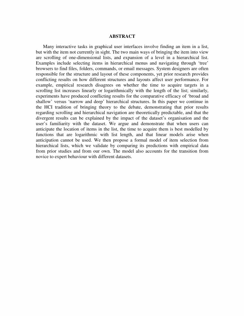
Figure 6. Calibrated parameters from the best-fit models for the different
conditions. Random order
T=a+b×items
Alphabetical order
T=a+b×log2(items+1)
Fitts/Flagged
T=a+b×log2(items+1)
a b R2 a b R
2 a b R
2
Non-scrolling
words
0.43 0.12 0.99 -0.17 0.44 0.99 0.24 0.13 0.96
Scrolling words -2.4 0.19 0.99 -5.13 1.28 0.99 -0.59 0.33 0.99
Word-ranges 1.45 0.29 0.99 -0.06 0.86 0.99
5. A MODEL OF HIERARCHICAL NAVIGATION
In navigating to a target through a hierarchy, the user carries out a series of selections, each of which is similar to the four-step list selection process described earlier. The structure of the dataset at each level may be the same or different, and hence a different model may be necessary for each hierarchical level. Figure 7 exemplifies this process within Windows Explorer with the user navigating from ‘Desktop’ and its arbitrarily ordered contents (Figure 7a), through the largely unpredictable contents of ‘My

Computer’ (Figure 7b) to ‘Network Drive H’ (Figure 7c), then scrolling through the alphabetical ordered items (Figure 7c) to the folder titled ‘paper’, then scrolling again through the numerically ordered list to ‘2007’ (Figure 7d,e), and on to the final target. Naturally, over time users can learn the location of items that are initially arbitrarily ordered, and our model will attempt to capture this process of transition from novice to expert performance.
Figure 7. Example hierarchical navigation through differently ordered levels within
Microsoft Windows Explorer.
(a) 1st level unpredictable. (b) 2
nd level
unpredictable.
(c) 3rd
level alphabetic.
(d) 4th
level numeric. (e) 5th
level alphabetic.
The performance model for hierarchical navigation predicts that the time Ti to select leaf node i at hierarchical depth d is the sum of the subtask times TLli for each ancestor at level l as well as the final leaf level.
∑=
=
d
l
lii TLT1
Eq 10.

The average performance for a hierarchical navigation widget Tavg can then be calculated as the product of the probability (pi) of each leaf node (i) and its time cost.
∑=
=
n
i
iiavg TpT1
Eq 11.
Incorporating the probability of selections into the model allows it to predict performance for the highly skewed distributions that are typically seen in real use—for example, several studies (Hansen, Kraut and Farber 1984; Ellis and Hitchcock 1986; Greenberg and Witten 1993; Findlater and McGrenere 2004) have shown that command use frequency follows a Zipfian distribution (Zipf 1949). Zipf’s law states that the frequency of word use follows a power distribution; that is, a power-law function Pn ~1/n
a, where Pn is the frequency of the nth ranked word, and a is close to 1.
The formula for TLli at each level is based on the menu performance model presented in Cockburn et al. (2007), which interpolates between novice and expert performance models. This interpolation depends on the user’s experience with items at each level, eli.
itypeexpertliitypenovicelili MeMeTL ,,,,)1( +−= Eq 12.
Experience with each item at each level (eli) is represented by a value between 0 and 1, calculated from the number of item selections (tli):
)/11( lili te −= Eq 13.
In other words, on their first trial with an item at some level, performance is entirely modelled by the novice model, but as their experience with that item increases, they shift towards the expert model.
Finally, the models for Mnovice,type,i and Mexpert,type,i depend on how users interact with the data at that level, as previously discussed in the analysis of scrolling above. The models are either linear or logarithmic functions of the item/list distance, dependent on whether a ballistic impulse toward the target can be used. The parameters of the model at each level require calibration.
The use of different formulae for Mnovice,type,i and Mexpert,type,i allow the model to accommodate different learning curves for different behaviours. For example, Figures 7a,b show that the top two levels of this Windows Explorer hierarchy are essentially arbitrarily ordered, so the inexperienced user will have to visually search for the item to expand – the novices’ model at both levels will be a linear function of the number of items. However, with experience, users will learn the spatial location of the items they frequently interact with, and hence the expert model for interaction with these items will be modelled by a logarithmic function of spatial location acquisition. Levels 3, 4 and 5, depicted in Figures 7c,d,e, will allow novices to select items in time that is a logarithmic function of the number of items at that level, but with experience, users will make a

transition to a faster (but still logarithmic) function of spatial location once the relative position of items in the list is learned.
Note that the model makes four assumptions about the starting state of the hierarchy and the user’s interaction with it:
• the scrollbar is initially located at the top of the scrolling list;
• the user navigates downwards through the list to the item;
• they never unnecessarily expand an incorrect branch in the hierarchy;
• all hierarchical items in the list are initially contracted.
These assumptions and associated extensions to the model to accommodate their removal are discussed later in the paper.
6. PREDICTIONS FOR BROAD/SHALLOW VS NARROW/DEEP
STRUCTURES
In this section we compare our model’s predictions for different hierarchical structures with those of prior studies. Although differences in experimental method mean that we cannot expect to predict actual performance values, the trends should be consistent. It is important to reiterate that several prior studies on the efficacy of different structures (broad/shallow versus narrow/deep) have generated inconsistent results. We contend that these divergent results are explained by our model, which distinguishes between structures that do and do not allow the user to anticipate the location of items at each level of the hierarchy. In essence, much of the prior work has sought a global answer on “broad/shallow or narrow/deep” when, as we shall demonstrate, no such general answer exists – the user’s ability to anticipate item location at each level must be taken into account.
Like prior experiments, for simplicity, we predict performance in hierarchies that have the following properties:
• All target items are held at the lowest level of the hierarchy.
• All target items are equally probable.
• Data is ordered in the same way at all levels.
• Data items are accessed at most once each, eliminating the need to model increasing expertise.
• The hierarchies are displayed in a window that allows 40 items to be displayed before scrolling is necessary.

The predictions are calculated using the calibration parameters presented in Equations 4-9 and summarised in Figure 6. Source data for these predictions are available in a spreadsheet at: www.cosc.canterbury.ac.nz/~andy/publs/hierarchyModel/predictions.xls.
6.1. Predictions for the Miller/Kiger/Snowberry hierarchies
The related work section reviewed several studies comparing item acquisition in 64-item hierarchies using random ordering at each level (Miller 1981; Snowberry et al. 1983; Kiger 1984). Their results showed a U-shaped performance curve, with slow performance in the shallow (641) and deep (26) conditions, while the medium depth conditions (4×16, 16×4, 82, and 43) allowed faster performance with relatively little difference between them. Snowberry’s data is shown in Figure 8.
Figure 8 also shows the model’s predictions, which form the same U-shaped performance pattern observed with random orderings. Our predictions for the random condition correlate well with Snowberry’s data for random organisations (linear r=0.96). For alphabetical orderings the flat 641 condition is predicted to allow faster acquisition than the other structures, and again, this prediction matches Snowberry et al.’s (1983) finding that their flat ‘categorised 64’ condition outperformed all others, leading them to advocate broad structures for strongly categorized data.
Figure 8. Predicted acquisition times for the 64 item structures evaluated in (Miller
1981; Snowberry et al. 1983; Kiger 1984), accurately reflecting the trends
observed in their studies. Snowberry’s data for the random condition is
also shown.
0
2
4
6
8
10
12
2^6 4^3 8^2 64^1
Hierarchical structure
Ac
qu
isit
ion
tim
e (
se
c)
Alpha - predicted
Random - predicted
Snowberry - Random
Snowberry - CAT64
6.2. Predictions of the Landauer and Nachbar hierarchies
Landauer and Nachbar (1985) empirically measured acquisition times to one of 4096 items in various hierarchies (212, 46, 84 and 163), with items alphabetically ordered at each level. We extracted their data from Figure 2 of their paper, and it is displayed in Figure 9a. Figure 9 also shows our model’s predictions for both alphabetical (Figure 9a) and random (Figure 9b) orderings, as well as a 642 structure which Landauer and Nachbar did not evaluate.

Analysis of Landauer and Nachbar’s empirical data against our predictions for the same alphabetical conditions shows a very strong correlation (r>0.99).
Interestingly, though, our model predicts a marked performance difference between random and alphabetic orderings in the 642 condition, with this broad condition outperforming all others with alphabetically sorted data (Figure 9a) but performing very poorly with unsorted data (Figure 9b). We are unaware of prior studies that have examined either condition.
7. TESTING THE MODEL
The previous section showed that the model’s predictions agree with the trends observed in previous studies. Although the trends are supported, there is as yet no evidence regarding the model’s accuracy in large structures that exhibit performance that is predicted to degrade linearly with length at each level (Landauer and Nachbar evaluated sorted data only), nor of the model’s predictions of the transition between novice and expert performance.
Figure 9. Predicted times for various alphabetically (left) and randomly (right)
ordered structures of 4096 items. Empirical data from Landauer and
Nachbar’s alphabetical conditions are also shown (left).
(a) Alphabetic structures (b) Random structures
0
5
10
15
20
25
30
2^12 4^6 8^4 16^3 64^2
Hierarchical structure
Ac
qu
isit
ion
tim
e (
se
c)
Alpha (Landauer & Nachbar)
Alpha Predicted
0
5
10
15
20
25
30
2^12 4^6 8^4 16^3 64^2
Hierarchical structure
Ac
qu
isit
ion
tim
e (
se
c)
Random Predicted
This section reports an experiment that tests two aspects of the model. First, we compared the predictions with actual performance, using a superset of the 4096-item Landauer and Nachbar structures with both random and alphabetical orderings, which should exhibit linear and logarithmic performance respectively at each level. All items were equally probable, and each item was accessed only once, negating the need to model performance improvement over trials. Second, we tested the predictions of the transition from novice to expert performance with repeated target acquisitions. In this case we used two of Miller’s structures of 64 items, randomly ordered, with a Zipfian distribution of item probability. According to our model, performance across trials should shift from visual search that is linear with length toward spatial acquisition that is logarithmic.

All tasks involved navigating to a specific five-letter word target through different hierarchical structures. All leaf nodes were held at the same (deepest) level of the hierarchy. When participants selected the correct leaf node, an audible confirmation tone was played and the screen cleared in preparation for the next task. Incorrect selections of leaf nodes produced an error tone, and the task continued until the correct item was selected. To reduce the impact of following incorrect paths, the error tone was also played if the participants expanded an incorrect node in the hierarchy.
Non-leaf nodes in the list showed the alphabetical range of words contained in the lower levels, for example “bungs – carry” at the top of Figure 10a or “lupus – zymes” at the top of Figure 10b.
7.1. Procedure
All participants completed tasks in the 4096 item structures before proceeding to the 64 item tasks.
Figure 10. The interface used in the final experiment.
(a) The alphabetic 642 condition. (b) The random 2
12 condition.
7.1.1. Tasks using Landauer and Nachbar’s 4096-item structures
Five structures of 4096 items were used – 212, 46, 84, 163 (as used by Landauer and Nachbar), and additionally 642. Items at each level of the hierarchy were either all random or all alphabetic. Even-numbered participants completed all five randomly ordered structures before proceeding to the five alphabetically ordered ones; and vice-versa for odd-numbered participants. Prior to completing experimental tasks with each

ordering, the participants were familiarised with the task by first browsing a 162 structure, then completing five training tasks within in it (data discarded). The order of the five structures for each participant was determined by an incomplete Latin square. Tasks were administered in ten blocks: five blocks, one for each structure, with the first first order (random or alphabetical), then another five with the second order. Each block consisted of five tasks, with one target at each of 17, 33, 50, 66 and 83% through the flattened structure. Each block began by repopulating the structure with a randomly selected set of words from the 7560 words used in the calibration experiment. The order of the five tasks in each block was randomly selected.
7.1.2. Repeated tasks in 64-item structures
These tasks are intended to reveal the transition from novice to expert performance when using a Zipfian distribution of item probabilities. Two randomly ordered but stable (i.e., items remained in a constant location) structures were used: 641 and 82. The 641 structure was used because, although predicted to be initially inefficient, it should improve rapidly as the user learns the location of items. The 82 was used because it is predicted to be relatively fast throughout.
Even numbered participants completed tasks using the 641 structure first; odd numbered participants, 82 first. For each participant with each structure, the 64 items were randomly selected. These items were then randomly ordered in the 641 structure. In the 82 structure the items were segregated into eight alphabetically ordered groups, which were randomly ordered at the top-level and the items contained within each range were randomly ordered at the second-level. Having established the randomly selected and arranged hierarchical structure for each participant, the structure remained stable throughout four blocks of tasks with that structure.
Each of the four blocks consisted of fifteen selections of six different items following a Zipfian frequency distribution (R2
=0.95): six selections of the 12th item, three of the 32nd, two of the 9th, two of the 28th, one of the 45th, and one of the 52nd. The assignment between location and frequency was determined by a random process. Each target item was randomly selected from the remaining block tasks.
7.2. Apparatus
The experiment ran on a Dell Precision 650 Xeon 3.2 GHz computer with a 17-inch
1280×1024 pixel LCD display and an optical mouse. The software was written in Tcl/Tk.
7.3. Participants
The thirteen participants (five female) were all undergraduate students from seven different majors. Their mean age was 24.1 years, and their mean reported hours per week of computer use was 38. They volunteered to participate in response to an email message sent to students enrolled in a psychology class. They received $10 compensation.

7.4. Results
The predictions for all conditions were calculated using the models presented in Equations 10-13, and summarised in Figure 6 (spreadsheet available at www.cosc.canterbury.ac.nz/~andy/hierarchyModel/predicitons.xls). The constants in these models (Figure 6) were calibrated in tasks involving top-level selections in which n
items or item-ranges were randomly selected from a set of 7560 words that spanned the entire alphabet. Hence, the average alphabetic range between words in the calibration experiment was 7560/n letters. This represents a ‘best case’ performance scenario where items can be discriminated alphabetically within the first one or two characters of the words on display. For example, Figure 10b shows that with n=2 when seeking ‘shawm’ the user’s first choice is between broad alphabetic ranges ‘abaca-lupin’ and ‘lupus-zymes’. At lower levels, however, the range between words is reduced to 7560/nl
(where l is the choice level) and hence the user needs to use the third, fourth or fifth letters to select the correct candidate: for example, choosing between ‘shape-sharp’ and ‘shave-sheaf’ (Figure 10b). Landauer and Nachbar’s empirical data reflects this trend of increasing difficulty with depth.
We therefore anticipate that our predictions will be low, but that the relative performance of different structure will be correct. Issues of calibration accuracy are further discussed later in the paper.
7.4.1. Tasks using Landauer and Nachbar’s 4096-item structures
Figure 11 shows the predicted and empirical mean times for the five structures in alphabetic (Figure 11a) and random (Figure 11b) orders. Although the predictions are low in all cases, the trends closely align with measured performance. Regression analyses of the predicted and empirical values show strong linear relationships between them: for the
alphabetic condition, Empirical=2.5×Predicted-6.5, R2=0.96; and for the random
condition, Empirical=1.05×Predicted+12.2, R2>0.99.
The following findings are important. First, in the alphabetic conditions, where users are able to anticipate the location of items in the data set at each level, the empirical data confirms the prediction that the broadest structures allow the best performance. Second, when data is ordered in a manner that prohibits anticipation (random in our case) the relative performance of different structures is more complex, but still predictable. The broadest 642 condition performed worst, closely followed by the narrowest 212 condition (consistent in both the prediction and the empirical data). The ‘U-shaped’ performance function observed in prior studies (Miller 1981; Snowberry et al. 1983; Kiger 1984) was also both predicted and confirmed, with similar performance in the 46, 84 and 163 conditions.

Figure 11. Predicted and empirical times for various structures of 4096 items.
(a) Alphabetic predictions and empirical
data (including results from Landauer
and Nachbar’s alphabetic conditions).
(b) Random predictions and empirical
data.
0
5
10
15
20
25
30
35
2^12 4^6 8^4 16^3 64^2
Hierarchical structure
Ac
qu
isit
ion
tim
e (
se
c)
Alpha ActualLandauer and NachbarAlpha Predicted
0
5
10
15
20
25
30
35
40
45
50
2^12 4^6 8^4 16^3 64^2
Hierarchical structure
Ac
qu
isit
ion
tim
e (
se
c)
Random ActualRandom Predicted
Further insights into performance are available by plotting the cumulative time taken to navigate through the structure levels, as shown in Figure 12. Four features of these plots are worth noting. First, although the scales differ between the predicted and empirical data (top row of Figure 12 for alphabetic, bottom row for random), the trends through the levels are similar. Second, while the predictions increase linearly for each condition through depth, the empirical data shows that successive choices are progressively slower at each level (the plots curve slightly upwards) until the last level or two. This effect was also noted by Landauer and Nachbar (Figure 12a). Third, the final levels of depth in the 212 condition show a slight reduction in choice time, causing a flattening of the performance curve (Figures 12c,e). This is explained by the high probability of the ultimate target appearing within the label for the deepest levels (for example, Figure 10b shows that the target ‘shawm’ appears at both the 11th and 12th levels, and often the target will also appear in the labels of the 9th or 10th levels too). Finally, it is interesting that even the first level of selection is slower than predicted. This is surprising because the conditions used to calibrate the predictions were precisely the same as those used to select the first level of the hierarchical structures. We believe this effect is due to experimental fatigue. The calibration experiment consisted of ten minutes of concentrated tasks, while the final experiment lasted roughly fifty minutes. Although participants were encouraged to take frequent breaks during the main experiment, several commented on the high levels of concentration required by the tasks.
7.4.2. Repeated tasks in 64-item structures
The predictions and empirical data from the 4096-item study examine the model’s effectiveness for comparing different structures with different data organisations. They do not, however, provide insight into whether the model accurately reflects the users’ transition from novice to expert performance as they gain experience with items.

Figure 12. Cumulative time to target as the number of choices remaining decreases
from 4096 to 1. Alphabetic conditions top (a, b, c), random conditions
bottom (d, e).
(a) Landauer and Nachbar
alphabetic (reproduced
from Figure 2 of their
paper).
(b) Alphabetic predicted. (c) Alphabetic empirical.
0
3
6
9
12
15
4096
2048
1024
512 256 128 64 32 16 8 4 2 1
Number of choices remaining
2
4
8
16
64
0
6
12
18
24
30
4096
2048
1024
512 256
128 64 32 16 8 4 2 1
Number of choices remaining
2
4
8
16
64
(d) Random predicted. (e) Random empirical.
0
5
10
15
20
25
30
35
4096
2048
1024 51
225
612
8 64 32 16 8 4 2 1
Number of choices remaining
Cu
mu
lati
ve
re
sp
on
se
tim
e (
se
c)
2
4
8
16
64
0
5
10
15
20
25
30
35
40
45
50
4096
2048
1024 51
225
612
8 64 32 16 8 4 2 1
Number of choices remaining
Cu
mu
lati
ve
re
sp
on
se
tim
e (
se
c)
2
4
8
16
64
Figure 13 shows the model’s predictions across blocks for the two random structures tested: 641 and 82. Solid lines in the figure show the empirical data; dashed ones, predicted. The predictions accurately follow the trends of the empirical data. Linear regression of predicted against empirical data for 641 gives a best-fit model of
Empirical=1.55×Predicted+0.81, R2=0.94. For the 82 condition the model is
Empirical=1.64×Predicted+0.25, R2=0.98.
The important aspects of Figure 13 are as follows. First, both prediction and empirical data show a marked performance advantage for 82 over 641 in the first block when users are most reliant on visual search. Performance improves across blocks due to users refining their spatial memory of item location – from visual search that is linear with length to spatial acquisition that is logarithmic. The empirical data also confirms the prediction that there is little performance difference between 82 and 641 once the users are experienced.
×
×
×
×
×
×
×
×
×
×
××
×
�
�
�
�
�
�
�
+
+
+
+
+�
�
�
�
248
16
4096 1024 256 64 32 16 8 4 2 1
5
10
15
20
25
Cu
mu
lati
ve
re
sp
on
se t
ime
(se
c)
Number of choices remaining
×
×
×
×
×
×
×
×
×
×
××
×
�
�
�
�
�
�
�
+
+
+
+
+�
�
�
�
248
16
4096 1024 256 64 32 16 8 4 2 1
5
10
15
20
25
Cu
mu
lati
ve
re
sp
on
se t
ime
(se
c)
Number of choices remaining
×
×
×
×
×
×
×
×
×
×
××
×
�
�
�
�
�
�
�
+
+
+
+
+�
�
�
�
248
16
4096 1024 256 64 32 16 8 4 2 1
5
10
15
20
25
Cu
mu
lati
ve
re
sp
on
se t
ime
(se
c)
Number of choices remaining

Figure 13. Predicted and empirical times across blocks of repeated trials for two
randomly ordered structures of 64 items: 82 and 64
1.
0
1
2
3
4
5
6
7
8
9
10
1 2 3 4
Block number
Ac
qu
isit
ion
tim
e (
se
c)
64-actual
64-predicted
8-actual
8-predicted
8. GENERAL DISCUSSION AND CONCLUSIONS
8.1. Accuracy of the model
There are two ways that our predictions differed from the empirical data: first, the predicted selection times were consistently low compared to real data; and second, the predicted time per choice did not gradually increase with depth (the slight curves apparent in Figures 12a,c,e).
Figures 8-13 show that although the model accurately discriminates between different designs, its absolute predictions are low, by up to 50% of the empirical value. Where does this inaccuracy come from, and why can we not account for it in the model? As mentioned above, we believe that there are two main reasons for the low predictions. First, the main empirical study involved approximately fifty minutes of intensive decision making, causing fatigue that was not present in the calibration study. Second, the hierarchical tasks involved an increasing task difficulty with depth, which also was not present in the calibration study.
The fatigue effect was clear from observation of the participants and from their comments. The tasks involved monotonous sequences of rapid decisions, and some participants had difficulty staying focused. Tasks in the randomly ordered conditions and in the deep conditions were particularly difficult and tiring. In contrast, the calibration data was gathered in short tasks that only involved the top level of the hierarchy.
Although we believe the fatigue effect was strong, we do not feel that it would be valuable to add terms to the model to account for it. Real-world users are very unlikely to carry out repeated selections in the way that our participants did. In addition, we believe

that a simpler model is easier for designers to work with, and fatigue is a factor that would be difficult to model well. This means that we must rely on the designer’s intuitions about the users and the task domain when interpreting the absolute values predicted by the model (and note that this issue does not affect the value of the model for purposes of comparing different designs or data organisations).
The second reason for our low predictions concerns the use of different linear models at each level of the hierarchy. As discussed earlier (and as can be seen in Figures 12b and 12d), our model uses the same calibration values for linear search at each level of the tree, whereas in the empirical study, the search task becomes slightly more difficult as the word range narrows at each level.
It is reasonable to consider whether we should add this increasing difficulty into the model, by adding different linear constants at each successive level. In the case of predicting the type of widget that was tested in our empirical study, this would involve recalibrating for each different linear difficulty level; and while this would provide a more accurate prediction, our focus here is more on determining the differences between different data organisation than on exact prediction. The current inaccuracy, then, is not a weakness of the underlying model; rather it is a reflection of the fact that different constants are required to calibrate for different types of data.
Does this mean that designers must do extensive calibration work in order to get accurate predictions? Would this simply shift the burden of empirical validation from one hand to the other, and require that designers still carry out user studies, but now in service of calibration rather than explicit testing of different designs? There are good reasons to believe that this is not as large a problem as it might seem. First, even if designers do carry out calibration studies, these are much simpler and faster than empirical design comparisons. Second, and more importantly, there are not that many variations on data organisation in hierarchical lists, and this suggests that a reasonably small set of parameter values would cover a wide range of possible designs. This process of establishing accepted norms for specific parameters is exemplified by the Fitts’ Law a and b parameters for mouse input, which have settled to values around 200ms for a and 0.2-0.27s/bit for b (values from Soukoreff and MacKenzie’s (2004) review of Fitts’ Law studies, reporting a throughput mouse range of 3.7-4.9bps, where throughput=1/b).
There are relatively few predictable data organisations that require parameterisation: alphabetic, numeric, chronological, and spatially known. In the case of unordered data (e.g., symbols), the calibration for random data can be used; and since unordered data cannot be organized into ranges, the top-level models are all that is needed.
8.2. Generalising from lists to any spatial layout
Although we have only considered list data organisations to date, we strongly suspect that the model will hold for two- or three-dimensional structures such as toolbar controls, desktop icon layouts (ordered or random), and nested dialogue boxes. Again, we contend that designers should be able to anticipate whether users’ performance with a structure will be linear or logarithmic with number of items. For example, searching for a word in

a paper dictionary involves navigating through a 3D structure, yet intuitively we can anticipate that time to find words will increase logarithmically with dictionary length.
Microsoft’s replacement of menus with the “ribbon” of tabbed toolbars in Office 2007 provides an interesting test-bed for this theory, which we intend to pursue. When users make the transition from traditional menus to the ribbon design, they will be reliant on visual search to find items (linear with n), but with experience they should gradually move toward performance that is logarithmic with the number of items. However, this transition is likely to be frustrated by the instability of items displayed in the ribbon, caused by the elision of contextual items (e.g. picture controls are only available when a picture is selected, causing other items to move location).
8.3. How can the model be used by designers?
The model allows us to reason about and predict the performance of different designs, answering a variety of questions that designers may have about their interfaces. There are two main ways that the model can be integrated into the design process: first, by more carefully considering the idea of data organisation; and second, by using the model to compare prospective designs, both in specific situations and across several variables.
8.3.1. The ideas of data organisation and stability
The model is grounded in the effects of different ways that list data can be organized, and in the degree of familiarity that the different organisations provide. The basic idea that familiar layouts will be faster than unfamiliar ones seems obvious, but there are sufficient real-world examples to suggest that the principle is still not widely applied. In particular, one specific type of organisation that we feel could be improved upon is organisation by order of creation – which can be seen in browser bookmark lists, Windows Explorer, and the program list under the Windows XP ‘Start’ menu. Although this organisation is not random, it is unfamiliar, since users are unlikely to maintain a sense of the order of addition. Another type of organisation that seems problematic is organisation by semantic category – if the user does not know the categories, then this layout is unfamiliar. The problem is that when new to the list, users have no effective fallback search strategy, and must resort to linear visual inspection, which is both slow and frustrating.
The frustration and effort effects are perhaps even more important than the performance impairment: anyone who has been unable to find a file in an Explorer window, or who has been unable to see a program group in Windows’ Programs menu, can attest to the degree of disruption that unfamiliar layouts can cause (e.g., find “FSViewerSetup28.exe” in Figure 14). Windows Explorer provides a variety of layouts to suit individual tastes, which is legitimate, but we believe that many problems could be solved by using alphabetic lists as the default.
A second idea that greatly affects familiarity is that of layout stability – and this too should be more consistently applied by interface designers. Our studies (and others) show

that stable layouts – even random organisations – very quickly lead to familiarity for those items that are frequently selected. Two principles can be drawn out of this idea. First, that stability is a good idea whatever overall organisation is chosen, and that dynamically changing the organisation is very probably a bad idea. Second, that the value of stability is highly dependent on item frequency, and that unfamiliar layouts, even stable ones, will still be difficult for users who are new to the list, or for items that are infrequent.
There is an interesting potential dilemma here in data spaces that are spatial and that evolve slowly over time. For example, icons on the desktop are usually organized by order of creation or by the user’s own semantic categories; if this layout remains stable, it can lead to a familiar (and fast) spatial understanding. However, there are always icons on the desktop that are used infrequently, and are hard to find. Again, we will investigate the validity of the model in 2D and 3D data representations in future work.
8.3.2. Comparing prospective designs
The second main way that designers can use the model is to compare prospective designs. The equations given above can predict performance for a given situation as long as the designer knows the basic elements that are part of the model: the data organisation, the number of levels in the hierarchy, the number of items at each level, and the size of the window (to determine how often the user needs to scroll in order to find the item of interest).
The most important element, as described above, is the data organisation and the user’s familiarity with that organisation. In some cases, the prospective designs will have exactly the types of organisation that we used (e.g., alphabetic or random), and the equations can be used as they stand; an example of this situation is given in Section 8.3.3.
In other situations where familiarity is different (e.g., the user has started to learn a random layout) the designer will need to determine new calibration parameters to account for an organisation that lies between our chosen exemplars. Similarly, there are many possibilities for systems and widgets to use novel design elements that are not explicitly part of the model presented here: for example, novel organisations of the data, combinations of two types of organisation, or visualization techniques to assist navigation. In these situations, designers cannot simply plug numbers in to the equations. Nevertheless, the model is still valuable as a guideline, and in these cases the designer can do a small amount of work to determine the major components of the design and how those should be combined using the basic terms and equations of the model. This approach is not difficult, and we have used it to model two complex designs (split menus and morphing menus) in previous work (Cockburn et al. 2007).
Another way that the comparative power of the model can be used is to find the best or worst possible conditions for a particular list design, or the boundaries between two designs. The model can be used to compare designs in a wide variety of possible cases – essentially running multiple individual comparisons at each level of a number of factors. This can determine whether there are any conditions where one design would outperform

another, and can also determine the possible worst-case scenario for a design. For example, a simulation study could show whether broad alphabetic organisations are more efficient than shallow categorical layouts, at any number of items and any depth of hierarchy.
Figure 14. Organisation by time of addition (and partially by semantics, in that files
and folders are grouped).
8.3.3. A Worked Example
As an example of how the model can be used, we consider the effects of changing the design of a file-system viewer. In particular, what would be the effect on performance of changing all Explorer windows in Figure 7 to alphabetic layouts? As described above, Windows Explorer in some cases presents layouts that are unfamiliar to the user, and in other cases presents items in alphabetic or numeric order.
We assume the window can show 40 items without scrolling, that all items are equally probable, that the hierarchy has five levels as shown in Figure 7, and that all item selections are made at the fifth level of the hierarchy. We calculate and compare the performance of three designs (all levels having unfamiliar organisation, the current strategy as depicted in Figure 14, and a fully alphabetized design) for 1 to 100 items.
Equations 3, 4, 6, 7 and 10 are used as functions in a spreadsheet to calculate performance for each number of items from 1 to 100 (spreadsheet available at www.cosc.canterbury.ac.nz/~andy/hierarchyModel/workedExample.xls). As shown in Figure 15, the performance differences are minor when there are fewer than about 10 items at each level, but become substantial when there are more than 20 items at each level: for example, at 40 items, the difference between alphabetic organisation and the original design is more than 6 seconds per selection (a 36% reduction); at 60 items, the difference is more than 11 seconds (47% reduction).

Figure 15. Predicted selection performance of three file-system viewer designs, by
number of items.
0
10
20
30
40
50
60
70
80
0 10 20 30 40 50 60 70 80 90 100
Number of items
Me
an
se
lect
ion
tim
e (
s)
random
mixed:2 random, 3 alpha
alpha
In this scenario, the model easily and quickly shows the relationships between performance, data organisation, and number of items. The total time to create the spreadsheet was no more than 15 minutes, but the results of this exercise could have provided the designer with clear indicators about the likely outcome of different design approaches. Similar (and equally simple) spreadsheets could be created to explore the effects of increasing user familiarity with static organisations, variable branching factors at the different levels, or different hierarchy depths.
8.3.4. Will designers believe the predictions?
From a designer’s perspective, a model is only useful if it reduces their workload. If the predictions are in doubt, then they must carry out follow-up confirmation studies to test the predictions, and this is clearly no better than simply doing the empirical work in the first place.
There are two answers to this concern. First, as the model matures, there will be greater confidence in it: the example of Fitts’ law is useful here, since designers in most cases no longer question the predictions of standard Fitts’ equations. Second, the model can also be useful even in situations where a confirmatory empirical study is necessary; since the model can test a much wider range of situations than empirical work, it can show the areas of design space that are likely to be most interesting for the empirical work. For example, the model could show where a likely cross-over point would be for two designs, and empirical studies could look at a much smaller set of experimental conditions than if the designers had no prior information.

8.4. From empiricism to theory
Gaines (1991) presents a concise ‘BRETAM’ model of increasing maturity in the information sciences. It states that research advances from a Breakthrough (e.g. the invention of a new technology, such as Engelbart’s invention of the mouse) through Replication, where others re-implement and refine the technology, to Empiricism, where the emphasis is on measuring and comparing performance. Theory follows Empiricism, allowing performance data to be explained and predicted (e.g. the application of Fitts’ Law to interface pointing tasks (Card, English and Burr 1978)). Theories allow Automation of scientific data gathering and analysis (e.g. the TouchStone platform for designing and conducting Fitts’ Law studies (Mackay, Appert, Beaudouin-Lafon, Chapuis, Du and Fekete 2007)). Finally, once automated, the focus becomes cost reduction and quality improvement of what has become Mature technology.
Although mouse maturation provides a good example of the BRETAM process, there are many areas of HCI that are yet to progress beyond Empiricism. Furthermore, we anecdotally observe that an increasing proportion of CHI research uses empirical methods as the sole tool for investigating performance. Frustration with over-reliance on empiricism is apparent in Lieberman’s CHI-Fringe article entitled ‘The Tyranny of Evaluation’ (Lieberman 2003), which was carefully rebutted by Zhai (2003).
While theory is arguably out of vogue in HCI research (other than Fitts’ Law), it has a strong history. Formal theoretical models have been used to predict human performance with interfaces since Card, Moran and Newell’s (1983) seminal work. However, as John et al. (2004) and Vera et al. (2005) observe, models have not yet had a widespread impact, partly because of the difficulty of the modelling process, but also because there is research contention over some of the elemental components on which models can be based. For example, Seow (2005) provides an excellent review comparing the success of Fitts’ Law in HCI with the relative obscurity of the Hick-Hyman Law (Hick 1952; Hyman 1953).
Our model is based on the empirical performance characteristics of user action – the theory is derived from empiricism, rather than from bottom up reconstruction of human perceptual, cognitive and motor capabilities. Ultimately, we envision HCI models similar to “Big O” notation (Knuth 1997), which is widely used in computer science for comparing the theoretical efficiency of algorithms.
In our further work we will examine how well the model predicts performance in more general interaction scenarios, such as navigating through commands represented in toolbars, ribbons or menus and through the tabbed panes in dialogue boxes.
ACKNOWLEDGEMENTS
Many thanks to Jean-Daniel Fekete, the anonymous reviewers, and action editor Prof. Dick Pew for their helpful comments and recommendations. Thanks also to Colin Oullette for his assistance in conducting the experiments, and to all of the participants.

REFERENCES
Andersen, T. (2005). A Simple Movement Time Model for Scrolling. Extended Abstracts of ACM CHI 2005, Portland, Oregon, 1180-1183. ACM.
Byrne, M., John, B., Wehrle, N. and Crow, D. (1999). The Tangled Web We Wove: A Taskonomy of WWW Use. Proceedings of CHI'99 ACM Conference on Human Factors in Computing Systems, Pittsburgh, 544-551.
Card, S., English, W. and Burr, B. (1978). "Evaluation of mouse, rate-controlled isometric joystick, step keys, and text keys for text selection on a CRT." Ergonomics 21(8): 601-613.
Card, S., Moran, T. and Newell, A. (1983). The Psychology of Human-Computer Interaction, Lawrence Erlbaum Associates.
Cockburn, A., Gutwin, C. and Greenberg, S. (2007). A Predictive Model of Menu Performance. Proceedings of CHI'07: ACM Conference on Human Factors in Computing Systems, San Jose, CA, To appear. ACM Press.
Cockburn, A., Savage, J. and Wallace, A. (2005). Tuning and Testing Scrolling Interfaces that Automatically Zoom. Proceedings of CHI'05: ACM Conference on Human Factors in Computing Systems, Portland, Oregon, 71-80. ACM Press.
Ellis, S. and Hitchcock, R. (1986). "Emergence of Zipf's Law: Spontaneous Encoding Optimization by Users of a Command Language." IEEE Transactions on Man and Cybernetics SMC-16: 423-427.
Findlater, L. and McGrenere, J. (2004). A comparison of static, adaptive, and adaptable menus. Proceedings CHI'04 Conference on Human Factors in Computing Systems, Vienna, Austria, 89-96. ACM Press.
Fitts, P. (1954). "The Information Capacity of the Human Motor System in Controlling the Amplitude of Movement." Journal of Experimental Psychology 47: 381-391.
Gaines, B. (1991). "Modeling and Forecasting the Information Sciences." Information Sciences 3(22): 57-58.
Geven, A., Sefelin, R. and Tscheligi, M. (2006). Depth and breadth away from the desktop: the optimal information hierarchy for mobile use. Proceedings of the 8th conference on Human-computer interaction with mobile devices and services, Helskinki, Finland, 157-164.
Greenberg, S. and Witten, I. (1993). "Supporting Command Reuse: Empirical Foundations and Principles." International Journal of Man-Machine Studies 39: 353--390.

Hansen, S., Kraut, R. and Farber, J. (1984). "Interface Design and Multivariate Analyis of Unix commands." ACM Transactions on Office Information Systems 2(1): 42-57.
Hick, W. (1952). "On the rate of gain of information." Quarterly Journal of Experimental Psychology 4: 11-36.
Hinckley, K., Cutrell, E., Bathiche, S. and Muss, T. (2002). Quantitative Analysis of Scrolling Techniques. Proceedings of CHI'02 ACM Conference on Human Factors in Computing Systems, Minneapolis, Minnesota, 65-72.
Hyman, R. (1953). "Stimulus information as a determinant of reaction time." Journal of Experimental Psychology 45: 188-196.
Jacko, J. and Salvendy, G. (1996). "Hierarchical menu design: breadth, depth, and task complexity." Perceptual and Motor Skills 82: 1187-1201.
John, B., Prevas, K., Salvucci, D. and Koedinger, K. (2004). Predictive Human Performance Modeling Made Easy. Proceedings of CHI'04: ACM Conference on Human Factors in Computing Systems, Vienna, Austria, 455-462. ACM Press.
Kiger, J. (1984). "The Depth/Breadth Tradeoff in the Design of Menu-Driven Interfaces." International Journal of Man-Machine Studies 20: 201-213.
Knuth, D. (1997). The Art of Computer Programming. Reading, Massachusetts, Addison-Wesley.
Landauer, T. and Nachbar, D. (1985). Selection from alphabetic and numeric menu trees using a touch screen: Breadth, depth and width. Proceedings of CHI'85 Conference on Human Factors in Computing Systems II, 73-78.
Lane, D., Napier, H., Batsell, R. and Naman, J. (1993). "Predicting the Skilled Use of Hierarchical Menus With the Keystroke-Level Model." Human Computer Interaction 8(2): 185-192.
Larson, K. and Czerwinski, M. (1998). Web Page Design: Implications of Memory, Structure and Scent for Information Retrieval. Proceedings of CHI'98. ACM Conference on Human Factors in Computing Systems, Los Angeles, CA, 25-32. ACM Press.
Lieberman, H. (2003). The Tyranny of Evaluation. CHI Fringe.
Mackay, W., Appert, C., Beaudouin-Lafon, M., Chapuis, O., Du, Y. and Fekete, J. (2007). Touchstone: Exploratory Design of Experiments. Proceedings of CHI'07: ACM Conference on Human Factors in Computing Systems, San Jose, CA, 1425-1434. ACM Press.

Miller, D. (1981). The depth/breadth tradeoff in hierarhical computer menus. Proceedings of the Human Factors Society 25th Annual Meeting, Santa Monica, CA, 296-300. HFES.
O'Hara, K. and Sellen, A. (1997). A comparison of reading paper and on-line documents. Proceedings of CHI'97 ACM Conference on Human factors in Computing Systems, New York, NY, USA, 335-342.
Seow, S. (2005). "Information Theoretic Models of HCI: A Comparison of the Hick-Hyman Law and Fitts' Law." Human-Computer Interaction 20(3): 315-352.
Shannon, C. and Weaver, W. (1949). The mathematical theory of communications, Urbana: University of Illinois Press.
Snowberry, K., Parkinson, S. and Sisson, N. (1983). "Computer Display Menus." Ergonomics 26(7): 699-712.
Soukoreff, R. and MacKenzie, I. S. (2004). "Towards a standard for pointing device evaluation, perspectives on 27 years of Fitts' law research in HCI." International Journal of Human Computer Studies 61(6): 751-789.
Vera, A., John, B., Remington, R., Matessa, M. and Freed, M. (2005). "Automating Human-Performance Modeling at the Millisecond Level." Human-Computer Interaction 20(3): 225-265.
Zaphiris, P., Shneiderman, B. and Norman, K. (2002). "Expandable Indexes versus Sequential Menus for Searching Hierarchies on the World Wide Web." International Journal of Behaviour and Information Technology 21(3): 201-207.
Zhai, S. (2003). Evaluation is the worst form of HCI research except all those other forms that have been tried. CHI Fringe.
Zhai, S., Smith, B. and Selker, T. (1997). Improving Browsing Performance: A Study of Four Input Devices for Scrolling and Pointing Tasks. Proceedings of INTERACT'97: the sixth IFIP conference on Human Computer Interaction, 286-292.
Zipf, G. (1949). Human Behavior and the Principle of Least Effort: An Introduction to Human Ecology. Reading, Mass., Addison-Wesley.

FIGURE CAPTIONS
Figure 1. Interfaces using some combination of hierarchy and scrolling to select
commands or data items.
Figure 2. Cursor velocity during target acquisition. An initial high velocity open-
loop, or ‘ballistic’, phase of motion is followed by several closed-loop
corrective actions in the final stages of acquisition.
Figure 3. The list interface used in the calibration experiment.
Figure 4. Results of the random word and word-range conditions.
Figure 5. Results of the alphabetical word and word-range conditions.
Figure 6. Calibrated parameters from the best-fit models for the different
conditions.
Figure 7. Example hierarchical navigation through differently ordered levels within
Microsoft Windows Explorer.
Figure 8. Predicted acquisition times for the 64 item structures evaluated in (Miller
1981; Snowberry et al. 1983; Kiger 1984), accurately reflecting the trends
observed in their studies. Snowberry’s data for the random condition is
also shown.
Figure 9. Predicted times for various alphabetically (left) and randomly (right)
ordered structures of 4096 items. Empirical data from Landauer and
Nachbar’s alphabetical conditions are also shown (left).
Figure 10. The interface used in the final experiment.
Figure 11. Predicted and empirical times for various structures of 4096 items.
Figure 12. Cumulative time to target as the number of choices remaining decreases
from 4096 to 1. Alphabetic conditions top (a, b, c), random conditions
bottom (d, e).
Figure 13. Predicted and empirical times across blocks of repeated trials for two
randomly ordered structures of 64 items: 82 and 64
1.
Figure 14. Organisation by time of addition (and partially by semantics, in that files
and folders are grouped).
Figure 15. Predicted selection performance of three file-system viewer designs, by
number of items.


![Predictive Modeling of Human Behavior: Supervised Learning from Telecom Metadata [Doctoral Thesis Presentation]](https://img.dokumen.tips/doc/110x75/5a65e1fc7f8b9ad05e8b49d5/predictive-modeling-of-human-behavior-supervised-learning-from-telecom-metadata.jpg)