Embed Size (px)
Citation preview

A Practical Introduction to Tensor Networks:
Matrix Product States and Projected Entangled Pair States
Roman Orus ∗
Institute of Physics, Johannes Gutenberg University, 55099 Mainz,Germany
June 11, 2014
Abstract
This is a partly non-technical introduction to selected topics on tensor network methods,based on several lectures and introductory seminars given on the subject. It should be agood place for newcomers to get familiarized with some of the key ideas in the field, speciallyregarding the numerics. After a very general introduction we motivate the concept of tensornetwork and provide several examples. We then move on to explain some basics about MatrixProduct States (MPS) and Projected Entangled Pair States (PEPS). Selected details on someof the associated numerical methods for 1d and 2d quantum lattice systems are also discussed.
∗E-mail address: [email protected]
1
arX
iv:1
306.
2164
v3 [
cond
-mat
.str
-el]
10
Jun
2014

Contents
1 Introduction 3
2 A bit of background 3
3 Why Tensor Networks? 5
3.1 New boundaries for classical simulations . . . . . . . . . . . . . . . . . . . . . . . . 5
3.2 New language for (condensed matter) physics . . . . . . . . . . . . . . . . . . . . . 5
3.3 Entanglement induces geometry . . . . . . . . . . . . . . . . . . . . . . . . . . . . . 6
3.4 Hilbert space is far too large . . . . . . . . . . . . . . . . . . . . . . . . . . . . . . . 6
4 Tensor Network theory 8
4.1 Tensors, tensor networks, and tensor network diagrams . . . . . . . . . . . . . . . . 8
4.2 Breaking the wave-function into small pieces . . . . . . . . . . . . . . . . . . . . . . 11
5 MPS and PEPS: generalities 14
5.1 Matrix Product States (MPS) . . . . . . . . . . . . . . . . . . . . . . . . . . . . . . 14
5.1.1 Some properties . . . . . . . . . . . . . . . . . . . . . . . . . . . . . . . . . 15
5.1.2 Some examples . . . . . . . . . . . . . . . . . . . . . . . . . . . . . . . . . . 21
5.2 Projected Entangled Pair States (PEPS) . . . . . . . . . . . . . . . . . . . . . . . . 25
5.2.1 Some properties . . . . . . . . . . . . . . . . . . . . . . . . . . . . . . . . . 25
5.2.2 Some examples . . . . . . . . . . . . . . . . . . . . . . . . . . . . . . . . . . 29
6 Extracting information: computing expectation values 32
6.1 Expectation values from MPS . . . . . . . . . . . . . . . . . . . . . . . . . . . . . . 32
6.2 Expectation values from PEPS . . . . . . . . . . . . . . . . . . . . . . . . . . . . . 33
6.2.1 Finite systems . . . . . . . . . . . . . . . . . . . . . . . . . . . . . . . . . . 34
6.2.2 Infinite systems . . . . . . . . . . . . . . . . . . . . . . . . . . . . . . . . . . 36
7 Determining the tensors: finding ground states 40
7.1 Variational optimization . . . . . . . . . . . . . . . . . . . . . . . . . . . . . . . . . 41
7.2 Imaginary time evolution . . . . . . . . . . . . . . . . . . . . . . . . . . . . . . . . 42
7.3 Stability and the normalization matrix N . . . . . . . . . . . . . . . . . . . . . . . . 45
8 Final remarks 46
2

1 Introduction
During the last years, the field of Tensor Networks has lived an explosion of results in severaldirections. This is specially true in the study of quantum many-body systems, both theoreticallyand numerically. But also in directions which could not be envisaged some time ago, such as itsrelation to the holographic principle and the AdS/CFT correspondence in quantum gravity [1, 2].Nowadays, Tensor Networks is rapidly evolving as a field and is embracing an interdisciplinary andmotivated community of researchers.
This paper intends to be an introduction to selected topics on the ever-expanding field of TensorNetworks, mostly focusing on some practical (i.e. algorithmic) applications of Matrix ProductStates and Projected Entangled Pair States. It is mainly based on several introductory seminarsand lectures that the author has given on the topic, and the aim is that the unexperienced readercan start getting familiarized with some of the usual concepts in the field. Let us clarify now,though, that we do not plan to cover all the results and techniques in the market, but rather topresent some insightful information in a more or less comprehensible way, sometimes also tryingto be intuitive, together with further references for the interested reader. In this sense, this paperis not intended to be a complete review on the topic, but rather a useful manual for the beginner.
The text is divided into several sections. Sec.2 provides a bit of background on the topic.Sec.3 motivates the use of Tensor Networks, and in Sec.4 we introduce some basics about TensorNetwork theory such as contractions, diagrammatic notation, and its relation to quantum many-body wave-functions. In Sec.5 we introduce some generalities about Matrix Product States (MPS)for 1d systems and Projected Entangled Pair States (PEPS) for 2d systems. Later in Sec.6 weexplain several strategies to compute expectation values and effective environments for MPS andPEPS, both for finite systems as well as systems in the thermodynamic limit. In Sec.7 we explaingeneralities on two families of methods to find ground states, namely variational optimizationand imaginary time evolution. Finally, in Sec.8 we provide some final remarks as well as a briefdiscussion on further topics for the interested reader.
2 A bit of background
Understanding quantum many-body systems is probably the most challenging problem in con-densed matter physics. For instance, the mechanisms behind high-Tc superconductivity are still amystery to a great extent despite many efforts [3]. Other important condensed matter phenomenabeyond Landau’s paradigm of phase transitions have also proven very difficult to understand, inturn combining with an increasing interest in new and exotic phases of quantum matter. Examplesof this are, to name a few, topologically ordered phases (where a pattern of long-range entangle-ment prevades over the whole system) [4], quantum spin liquids (phases of matter that do notbreak any symmetry) [5], and deconfined quantum criticality (quantum critical points betweenphases of fundamentally-different symmetries) [6].
The standard approach to understand these systems is based on proposing simplified modelsthat are believed to reproduce the relevant interactions responsible for the observed physics, e.g.the Hubbard and t−J models in the case of high-Tc superconductors [7]. Once a model is proposed,and with the exception of some lucky cases where these models are exactly solvable, one needs torely on faithful numerical methods to determine their properties.
As far as numerical simulation algorithms are concerned, Tensor Network (TN) methods havebecome increasingly popular in recent years to simulate strongly correlated systems [8]. In thesemethods the wave function of the system is described by a network of interconnected tensors.Intuitively, this is like a decomposition in terms of LEGO R© pieces, and where entanglement plays
3

the role of a “glue” amongst the pieces. To put it in another way, the tensor is the DNA of the wave-function, in the sense that the whole wave-function can be reconstructed from this fundamentalpiece, see Fig.(1). More precisely, TN techniques offer efficient descriptions of quantum many-body states that are based on the entanglement content of the wave function. Mathematically,the amount and structure of entanglement is a consequence of the chosen network pattern and thenumber of parameters in the tensors.
Figure 1: (color online) (a) The DNA is the fundamental building block of a person. In thesame way, (b) the tensor is the fundamental building block of a quantum state (here we use adiagrammatic notation for tensors that will be made more precise later on). Therefore, we couldsay that the tensor is the DNA of the wave-function, in the sense that the whole wave-functioncan be reconstructed from it just by following some simple rules.
The most famous example of a TN method is probably the Density Matrix RenormalizationGroup (DMRG) [9, 10, 11, 12], introduced by Steve White in 1992. One could say that this methodhas been the technique of reference for the last 20 years to simulate 1d quantum lattice systems.However, many important breakthroughs coming from quantum information science have under-pinned the emergence of many other algorithms based on TNs. It is actually quite easy to getlost in the soup of names of all these methods, e.g. Time-Evolving Block Decimation (TEBD)[13, 14], Folding Algorithms [15], Projected Entangled Pair States (PEPS) [16], Tensor Renor-malization Group (TRG) [18], Tensor-Entanglement Renormalization Group (TERG) [17], TensorProduct Variational Approach [19], Weighted Graph States [20], Entanglement Renormalization(ER) [21], Branching MERA [22], String-Bond States [23], Entangled-Plaquette States [24], MonteCarlo Matrix Product States [25], Tree Tensor Networks [26], Continuous Matrix Product Statesand Continuous Tensor Networks [27], Time-Dependent Variational Principle (TDVP) [28], Sec-ond Renormalization Group (SRG)[29], Higher Order Tensor Renormalization Group (HOTRG)[30]... and these are just some examples. Each one of these methods has its own advantages anddisadvantages, as well as optimal range of applicability.
A nice property of TN methods is their flexibility. For instance, one can study a varietyof systems in different dimensions, of finite or infinite size [31, 14, 32, 33, 18, 29, 30, 34], with
4
different boundary conditions [11, 35], symmetries [36], as well as systems of bosons [37], fermions[38] and frustrated spins [39]. Different types of phase transitions [40] have also been studied inthis context. Moreover, these methods are also now finding important applications in the contextof quantum chemistry [41] and lattice gauge theories [42], as well as interesting connections toquantum gravity, string theory and the holographic principle [2]. The possibility of developingalgorithms for infinite-size systems is quite relevant, because it allows to estimate the properties ofa system directly in the thermodynamic limit and without the burden of finite-size scaling effects1.Examples of methods using this approach are iDMRG [31] and iTEBD [14] in 1d (the “i” meansinfinite), as well as iPEPS [32], TRG/SRG [18, 29], and HOTRG [30] in 2d. From a mathematicalperspective, a number of developments in tensor network theory have also come from the field oflow-rank tensor approximations in numerical analysis [43].
3 Why Tensor Networks?
Considering the wide variety of numerical methods for strongly correlated systems that are avail-able, one may wonder about the necessity of TN methods at all. This is a good question, for whichthere is no unique answer. In what follows we give some of the reasons why these methods areimportant and, above all, necessary.
3.1 New boundaries for classical simulations
All the existing numerical techniques have their own limitations. To name a few: the exact diago-nalization of the quantum Hamiltonian (e.g. Lanczos methods [44]) is restricted to systems of smallsize, thus far away from the thermodynamic limit where quantum phase transitions appear. Seriesexpansion techniques [45] rely on perturbation theory calculations. Mean field theory [46] failsto incorporate faithfully the effect of quantum correlations in the system. Quantum Monte Carloalgorithms [47] suffer from the sign problem, which restricts their application to e.g. fermionic andfrustrated quantum spin systems. Methods based on Continuous Unitary Transformations [48] relyon the approximate solution of a system of infinitely-many coupled differential equations. CoupledCluster Methods [49] are restricted to small and medium-sized molecules. And Density FunctionalTheory [50] depends strongly on the modeling of the exchange and correlation interactions amongstelectrons. Of course, these are just some examples.
TN methods are not free from limitations either. But as we shall see, their main limitation isvery different: the amount and structure of the entanglement in quantum many-body states. Thisnew limitation in a computational method extends the range of models that can be simulated witha classical computer in new and unprecedented directions.
3.2 New language for (condensed matter) physics
TN methods represent quantum states in terms of networks of interconnected tensors, which inturn capture the relevant entanglement properties of a system. This way of describing quantumstates is radically different from the usual approach, where one just gives the coefficients of a wave-function in some given basis. When dealing with a TN state we will see that, instead of thinkingabout complicated equations, we will be drawing tensor network diagrams, see Fig.(2). As such, ithas been recognized that this tensor description offers the natural language to describe quantumstates of matter, including those beyond the traditional Landau’s picture such as quantum spin
1We shall see that translational invariance plays a key role in this case.
5

liquids and topologically-ordered states. This is a new language for condensed matter physics (andin fact, for all quantum physics) that makes everything much more visual and which brings newintuitions, ideas and results.
Figure 2: (color online) Two examples of tensor network diagrams: (a) Matrix Product State(MPS) for 4 sites with open boundary conditions; (b) Projected Entangled Pair State (PEPS) fora 3× 3 lattice with open boundary conditions.
3.3 Entanglement induces geometry
Imagine that you are given a quantum many-body wave-function. Specifying its coefficients ina given local basis does not give any intuition about the structure of the entanglement betweenits constituents. It is expected that this structure is different depending on the dimensionality ofthe system: this should be different for 1d systems, 2d systems, and so on. But it should alsodepend on more subtle issues like the criticality of the state and its correlation length. Yet, naiverepresentations of quantum states do not possess any explicit information about these properties.It is desirable, thus, to find a way of representing quantum sates where this information is explicitand easily accessible.
As we shall see, a TN has this information directly available in its description in terms of anetwork of quantum correlations. In a way, we can think of TN states as quantum states given insome entanglement representation. Different representations are better suited for different typesof states (1d, 2d, critical...), and the network of correlations makes explicit the effective latticegeometry in which the state actually lives. We will be more precise with this in Sec.4.2. At thislevel this is just a nice property. But in fact, by pushing this idea to the limit and turning itaround, a number of works have proposed that geometry and curvature (and hence gravity) couldemerge naturally from the pattern of entanglement present in quantum states [51]. Here we willnot discuss further this fascinating idea, but let us simply mention that it becomes apparent thatthe language of TN is, precisely, the correct one to pursue this kind of connection.
3.4 Hilbert space is far too large
This is, probably, the main reason why TNs are a key description of quantum many-body statesof Nature. For a system of e.g. N spins 1/2, the dimension of the Hilbert space is 2N , whichis exponentially large in the number of particles. Therefore, representing a quantum state of themany-body system just by giving the coefficients of the wave function in some local basis is aninefficient representation. The Hilbert space of a quantum many-body system is a really big placewith an incredibly large number of quantum states. In order to give a quantitative idea, let usput some numbers: if N ∼ 1023 (of the order of the Avogadro number) then the number of basis
6

Figure 3: (color online) The entanglement entropy between A and B scales like the size of theboundary ∂A between the two regions, hence S ∼ ∂A.
states in the Hilbert space is ∼ O(101023
), which is much larger (in fact exponentially larger) thanthe number of atoms in the observable universe, estimated to be around 1080! [52]
Luckily enough for us, not all quantum states in the Hilbert space of a many-body systemare equal: some are more relevant than others. To be specific, many important Hamiltoniansin Nature are such that the interactions between the different particles tend to be local (e.g.nearest or next-to-nearest neighbors)2. And locality of interactions turns out to have importantconsequences. In particular, one can prove that low-energy eigenstates of gapped Hamiltonianswith local interactions obey the so-called area-law for the entanglement entropy [53], see Fig.(3).This means that the entanglement entropy of a region of space tends to scale, for large enoughregions, as the size of the boundary of the region and not as the volume3. And this is a veryremarkable property, because a quantum state picked at random from a many-body Hilbert spacewill most likely have a entanglement entropy between subregions that will scale like the volume,and not like the area. In other words, low-energy states of realistic Hamiltonians are not just“any” state in the Hilbert space: they are heavily constrained by locality so that they must obey theentanglement area-law.
By turning around the above consideration, one finds a dramatic consequence: it means that not“any” quantum state in the Hilbert space can be a low-energy state of a gapped, local Hamiltonian.Only those states satisfying the area-law are valid candidates. Yet, the manifold containing thesestates is just a tiny, exponentially small, corner of the gigantic Hilbert space (see Fig.(4)). Thiscorner is, therefore, the corner of relevant states. And if we aim to study states within this corner,then we better find a tool to target it directly instead of messing around with the full Hilbertspace. Here is where the good news come: it is the family of TN states the one that targets thismost relevant corner of states [57]. Moreover, recall that Renormalization Group (RG) methodsfor many-body systems aim to, precisely, identify and keep track of the relevant degrees of freedomto describe a system. Thus, it looks just natural to devise RG methods that deal with this relevantcorner of quantum states, and are therefore based on TN states.
In fact, the consequences of having such an immense Hilbert space are even more dramatic. Forinstance, one can also prove that by evolving a quantum many-body state a time O(poly(N)) witha local Hamiltonian, the manifold of states that can be reached in this time is also exponentiallysmall [58]. In other words: the vast majority of the Hilbert space is reachable only after a timeevolution that would take O(exp(N)) time. This means that, given some initial quantum state
2Here we will not enter into deep reasons behind the locality of interactions, and will simply take it for granted.Notice, though, that there are also many important condensed-matter Hamiltonians with non-local interactions,e.g., with a long-range Coulomb repulsion.
3For gapless Hamiltonians there may be multiplicative and/or additive corrections to this behavior, see e.g. Refs.[54, 55, 56].
7

Figure 4: (color online) The manifold of quantum states in the Hilbert space that obeys the area-law scaling for the entanglement entropy corresponds to a tiny corner in the overall huge space.
(which quite probably will belong to the relevant corner that satisfies the area-law), most of theHilbert space is unreachable in practice. To have a better idea of what this means let us put againsome numbers: for N ∼ 1023 particles, by evolving some quantum state with a local Hamiltonian,reaching most of the states in the Hilbert space would take ∼ O(101023
) seconds. Consideringthat the best current estimate for the age of the universe is around 1017 seconds [59], this meansthat we should wait around the exponential of one-million times the age of the universe to reachmost of the states available in the Hilbert space. Add to this that your initial state must also becompatible with some locality constraints in your physical system (because otherwise it may notbe truly physical), and what you obtain is that all the quantum states of many-body systems thatyou will ever be able to explore are contained in a exponentially small manifold of the full Hilbertspace. This is why the Hilbert space of a quantum many-body systems is sometimes referred to asa convenient illusion [58]: it is convenient from a mathematical perspective, but it is an illusionbecause no one will ever see most of it.
4 Tensor Network theory
Let us now introduce some mathematical concepts. In what follows we will define what a TNstate is, and how this can be described in terms of TN diagrams. We will also introduce the TNrepresentation of quantum states, and explain the examples of Matrix Product States (MPS) for1d systems [60], and Projected Entangled Pair States (PEPS) for 2d systems [16].
4.1 Tensors, tensor networks, and tensor network diagrams
For our purposes, a tensor is a multidimensional array of complex numbers. The rank of a tensoris the number of indices. Thus, a rank-0 tensor is scalar (x), a rank-1 tensor is a vector (vα), anda rank-2 tensor is a matrix (Aαβ).
An index contraction is the sum over all the possible values of the repeated indices of a set oftensors. For instance, the matrix product
Cαγ =
D∑β=1
AαβBβγ (1)
8

is the contraction of index β, which amounts to the sum over its D possible values. One can alsohave more complicated contractions, such as this one:
Fγωρσ =
D∑α,β,δ,ν,µ=1
AαβδσBβγµCδνµωEνρα , (2)
where for simplicity we assumed that contracted indices α, β, δ, ν and µ can take D different values.As seen in these examples, the contraction of indices produces new tensors, in the same way thate.g. the product of two matrices produces a new matrix. Indices that are not contracted are calledopen indices.
A Tensor Network (TN) is a set of tensors where some, or all, of its indices are contractedaccording to some pattern. Contracting the indices of a TN is called, for simplicity, contractingthe TN. The above two equations are examples of TN. In Eq.(1), the TN is equivalent to a matrixproduct, and produces a new matrix with two open indices. In Eq.(2), the TN corresponds tocontracting indices α, β, δ, ν and µ in tensors A,B,C and E to produce a new rank-4 tensor Fwith open indices γ, ω, ρ and σ. In general, the contraction of a TN with some open indices givesas a result another tensor, and in the case of not having any open indices the result is a scalar.This is the case of e.g. the scalar product of two vectors,
C =
D∑α=1
AαBα , (3)
where C is a complex number (rank-0 tensor). A more intrincate example could be
F =
D∑α,β,γ,δ,ω,ν,µ=1
AαβδγBβγµCδνµωEνωα , (4)
where all indices are contracted and the result is again a complex number F .
Once this point is reached, it is convenient to introduce a diagrammatic notation for tensors andTNs in terms of tensor network diagrams, see Fig.(5). In these diagrams tensors are represented byshapes, and indices in the tensors are represented by lines emerging from the shapes. A TN is thusrepresented by a set of shapes interconnected by lines. The lines connecting tensors between eachother correspond to contracted indices, whereas lines that do not go from one tensor to anothercorrespond to open indices in the TN.
Figure 5: (color online) Tensor network diagrams: (a) scalar, (b) vector, (c) matrix and (d) rank-3tensor
Using TN diagrams it is much easier to handle calculations with TN. For instance, the contrac-tions in Eqs.(1, 2, 3, 4) can be represented by the diagrams in Fig.(6). Also tricky calculations,like the trace of the product of 6 matrices, can be represented by diagrams as in Fig.(7). From theTN diagram the cyclic property of the trace becomes evident. This is a simple example of why TN
9

Figure 6: (color online) Tensor network diagrams for Eqs.(1, 2, 3, 4): (a) matrix product, (b)contraction of 4 tensors with 4 open indices, (c) scalar product of vectors, and (d) contraction of4 tensors without open indices.
Figure 7: (color online) Trace of the product of 6 matrices.
diagrams are really useful: unlike plain equations, TN diagrams allow to handle with complicatedexpressions in a visual way. In this manner many properties become apparent, such as the cyclicproperty of the trace of a matrix product. In fact, you could compare the language of TN diagramsto that of Feynman diagrams in quantum field theory. Surely it is much more intuitive and visualto think in terms of drawings instead of long equations. Hence, from now on we shall only usediagrams to represent tensors and TNs.
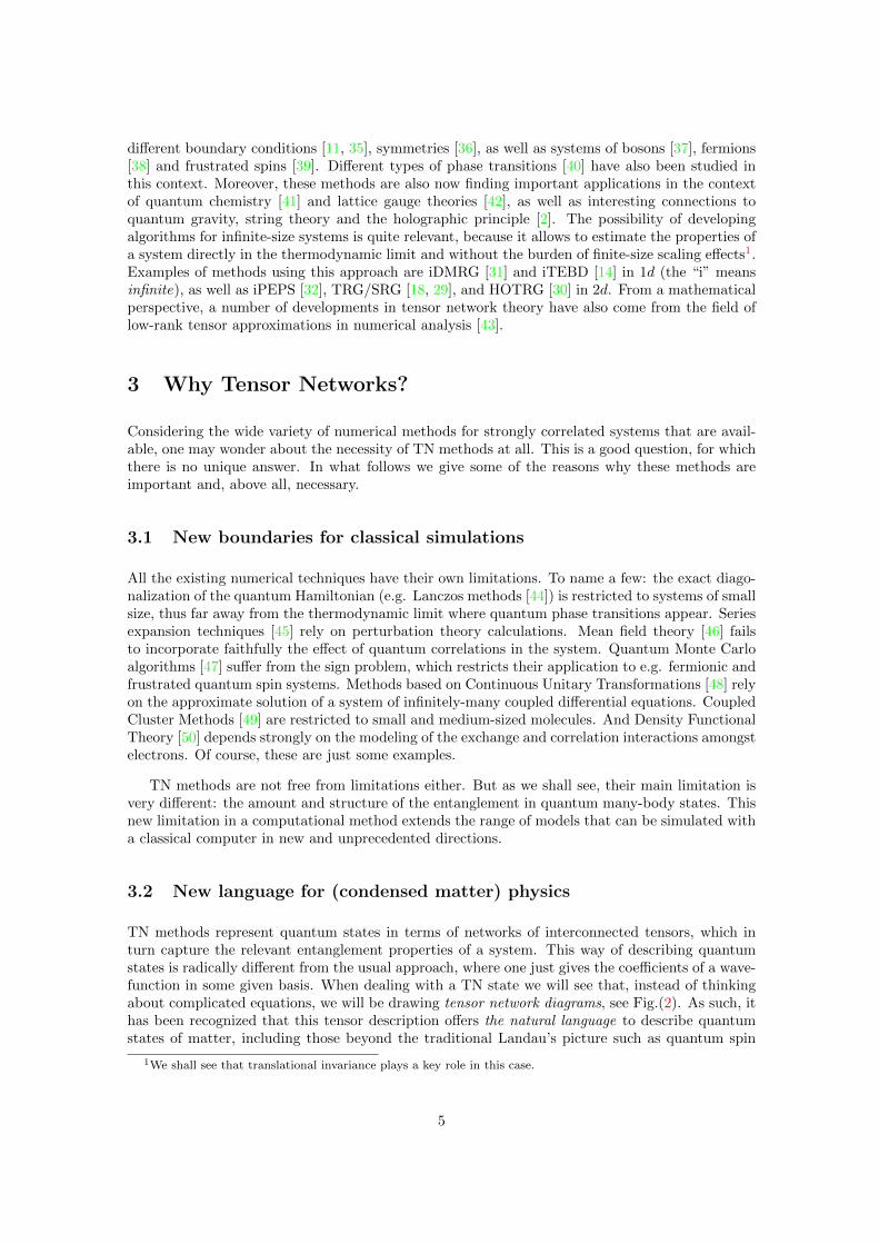
There is an important property of TN that we would like to stress now. Namely, that the totalnumber of operations that must be done in order to obtain the final result of a TN contractiondepends heavily on the order in which indices in the TN are contracted. See for instance Fig.(8).Both cases correspond to the same overall TN contraction, but in one case the number of operationsis O(D4) and in the other is O(D5). This is quite relevant, since in TN methods one has to dealwith many contractions, and the aim is to make these as efficiently as possible. For this, findingthe optimal order of indices to be contracted in a TN will turn out to be a crucial step, speciallywhen it comes to programming computer codes to implement the methods. To minimize thecomputational cost of a TN contraction one must optimize over the different possible orderings ofpairwise contractions, and find the optimal case. Mathematically this is a very difficult problem,though in practical cases this can be done usually by simple inspection.
10
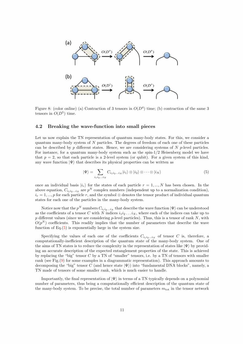
Figure 8: (color online) (a) Contraction of 3 tensors in O(D4) time; (b) contraction of the same 3tensors in O(D5) time.
4.2 Breaking the wave-function into small pieces
Let us now explain the TN representation of quantum many-body states. For this, we consider aquantum many-body system of N particles. The degrees of freedom of each one of these particlescan be described by p different states. Hence, we are considering systems of N p-level particles.For instance, for a quantum many-body system such as the spin-1/2 Heisenberg model we havethat p = 2, so that each particle is a 2-level system (or qubit). For a given system of this kind,any wave function |Ψ〉 that describes its physical properties can be written as
|Ψ〉 =∑
i1i2...iN
Ci1i2...iN |i1〉 ⊗ |i2〉 ⊗ · · · ⊗ |iN 〉 (5)
once an individual basis |ir〉 for the states of each particle r = 1, ..., N has been chosen. In theabove equation, Ci1i2...iN are pN complex numbers (independent up to a normalization condition),ir = 1, ..., p for each particle r, and the symbol ⊗ denotes the tensor product of individual quantumstates for each one of the particles in the many-body system.
Notice now that the pN numbers Ci1i2...iN that describe the wave function |Ψ〉 can be understoodas the coefficients of a tensor C with N indices i1i2 . . . iN , where each of the indices can take up top different values (since we are considering p-level particles). Thus, this is a tensor of rank N , withO(pN ) coefficients. This readily implies that the number of parameters that describe the wavefunction of Eq.(5) is exponentially large in the system size.
Specifying the values of each one of the coefficients Ci1i2...iN of tensor C is, therefore, acomputationally-inefficient description of the quantum state of the many-body system. One ofthe aims of TN states is to reduce the complexity in the representation of states like |Ψ〉 by provid-ing an accurate description of the expected entanglement properties of the state. This is achievedby replacing the “big” tensor C by a TN of “smaller” tensors, i.e. by a TN of tensors with smallerrank (see Fig.(9) for some examples in a diagrammatic representation). This approach amounts todecomposing the “big” tensor C (and hence state |Ψ〉) into “fundamental DNA blocks”, namely, aTN made of tensors of some smaller rank, which is much easier to handle.
Importantly, the final representation of |Ψ〉 in terms of a TN typically depends on a polynomialnumber of parameters, thus being a computationally efficient description of the quantum state ofthe many-body system. To be precise, the total number of parameters mtot in the tensor network
11

Figure 9: (color online) Tensor network decomposition of tensor C in terms of (a) an MPS withperiodic boundary conditions, (b) a PEPS with open boundary condition, and (c) an arbitrarytensor network.
will be
mtot =
Ntens∑t=1
m(t) , (6)
where m(t) is the number of parameters for tensor t in the TN and Ntens is the number of tensors.For a TN to be practical Ntens must be sub-exponential in N , e.g. Ntens = O(poly(N)), andsometimes even Ntens = O(1). Also, for each tensor t the number of parameters is
m(t) = O
rank(t)∏at=1
D(at)
, (7)
where the product runs over the different indices at = 1, 2, . . . , rank(t) of the tensor, D(at) is thedifferent possible values of index at, and rank(t) is the number of indices of the tensor. Calling Dt
the maximum of all the numbers D(at) for a given tensor, we have that
m(t) = O(D
rank(t)t
). (8)
Putting all the pieces together, we have that the total number of parameters will be
mtot =
Ntens∑t=1
O(D
rank(t)t
)= O(poly(N)poly(D)) , (9)
where D is the maximum of Dt over all tensors, and where we assumed that the rank of eachtensor is bounded by a constant.
To give a simple example, consider the TN in Fig.(9.a). This is an example of a Matrix ProductState (MPS) with periodic boundary conditions, which is a type of TN that will be discussed indetail in the next section. Here, the number of parameters is just O(NpD2), if we assume thatopen indices in the TN can take up to p values, whereas the rest can take up to D values. Yet, thecontraction of the TN yields a tensor of rank N , and therefore pN coefficients. Part of the magic
12

of the TN description is that it shows that these pN coefficients are not independent, but ratherthey are obtained from the contraction of a given TN and therefore have a structure.
Nevertheless, this efficient representation of a quantum many-body state does not come forfree. The replacement of tensor C by a TN involves the appearance of extra degrees of freedomin the system, which are responsible for “gluing the different DNA blocks” together. These newdegrees of freedom are represented by the connecting indices amongst the tensors in the TN. Theconnecting indices turn out to have an important physical meaning: they represent the structureof the many-body entanglement in the quantum state |Ψ〉, and the number of different values thateach one of these indices can take is a quantitative measure of the amount of quantum correlationsin the wave function. These indices are usually called bond or ancillary indices, and their numberof possible values are referred to as bond dimensions. The maximum of these values, which wecalled above D, is also called the bond dimension of the tensor network.
To understand better how entanglement relates to the bond indices, let us give an example.Imagine that you are given a TN state with bond dimension D for all the indices, and such as theone in Fig.(10). This is an example of a TN state called Projected Entangled Pair State (PEPS)[16], which will also be further analyzed in the forthcoming sections. Let us now estimate for thisstate the entanglement entropy of a block of linear length L (see the figure). For this, we callα = {α1α2...α4L} the combined index of all the TN indices across the boundary of the block.Clearly, if the α indices can take up to D values, then α can take up to D4L. We now write thestate in terms of unnormalized kets for the inner and outer parts of the block (see also Fig.(10)) as
|Ψ〉 =
D4L∑α=1
|in(α)〉 ⊗ |out(α)〉 . (10)
The reduced density matrix of e.g. the inner part is given by
ρin =∑α,α′
Xαα′ |in(α)〉〈in(α′)| , (11)
where Xαα′ ≡ 〈out(α′)|out(α)〉. This reduced density matrix clearly has a rank that is, at most,D4L. The same conclusions would apply if we considered the reduced density matrix of the outsideof the block. Moreover, the entanglement entropy S(L) = −tr(ρin log ρin) of the block is upperbounded by the logarithm of the rank of ρin. So, in the end, we get
S(L) ≤ 4L logD , (12)
which is nothing but an upper-bound version of the area-law for the entanglement entropy [53]. Infact, we can also interpret this equation as every “broken” bond index giving an entropy contributionof at most logD.
Let us discuss the above result. First, if D = 1 then the upper bound says that S(L) = 0 nomatter the size of the block. That is, no entanglement is present in the wave function. This isa generic result for any TN: if the bond dimensions are trivial, then no entanglement is presentin the wave function, and the TN state is just a product state. This is the type of ansatz thatis used in e.g. mean field theory. Second, for any D > 1 we have that the ansatz can alreadyhandle an area-law for the entanglement entropy. Changing the bond dimension D modifies onlythe multiplicative factor of the area-law. Therefore, in order to modify the scaling with L oneshould change the geometric pattern of the TN. This means that the entanglement in the TN is aconsequence of both D (the “size” of the bond indices), and also the geometric pattern (the waythese bond indices are connected). In fact, different families of TN states turn out to have verydifferent entanglement properties, even for the same D. Third, notice that by limiting D to a fixedvalue greater than one we can achieve TN representations of a quantum many-body state which
13

Figure 10: (color online) States |in(α)〉 and |out(α)〉 for a 4× 4 block of a 6× 6 PEPS.
are both computationally efficient (as in mean field theory) and quantumly correlated (as in exactdiagonalization). In a way, by using TNs one gets the best of both worlds.
TN states are also important because they have been proven to correspond to ground andthermal states of local, gapped Hamiltonians [57]. This means that TN states are, in fact, thestates inside the relevant corner of the Hilbert space that was discussed in the previous section:they correspond to relevant states in Nature which obey the area-law and can, on top, be describedefficiently using the tensor language.
5 MPS and PEPS: generalities
Let us now present two families of well-known and useful TN states. These are Matrix ProductStates (MPS) and Projected Entangled Pair States (PEPS). Of course these two are not the onlyfamilies of TN states, yet these will be the only two that we will consider in some detail here. Forthe interested reader, we briefly mention other families of TN states in Sec.8.
5.1 Matrix Product States (MPS)
The family of MPS [60] is probably the most famous example of TN states. This is because it isbehind some very powerful methods to simulate 1d quantum many-body systems, most prominentlythe Density Matrix Renormalization Group (DMRG) algorithm [9, 10, 11, 12]. But it is also behindother well-known methods such as Time-Evolving Block Decimation (TEBD) [13, 14] and Power
14

Wave Function Renormalization Group (PWFRG) [61]. Before explaining any method, though,let us first describe what an MPS actually is, as well as some of its properties.
MPS are TN states that correspond to a one-dimensional array of tensors, such as the ones inFig.(11). In a MPS there is one tensor per site in the many-body system. The connecting bondindices that glue the tensors together can take up to D values, and the open indices correspondto the physical degrees of freedom of the local Hilbert spaces which can take up to p values. InFig.(11) we can see two examples of MPS. The first one corresponds to a MPS with open boundaryconditions4, and the second one to a MPS with periodic boundary conditions [11]. Both examplesare for a finite system of 4 sites.
Figure 11: (color online) (a) 4-site MPS with open boundary conditions; (b) 4-site MPS withperiodic boundary conditions.
5.1.1 Some properties
Let us now explain briefly some basic properties of MPS:
1) 1d translational invariance and the thermodynamic limit.- In principle, all tensors ina finite-size MPS could be different, which means that the MPS itself is not translational invariant(TI). However, it is also possible to impose TI and take the thermodynamic limit of the MPS bychoosing some fundamental unit cell of tensors that is repeated over the 1d lattice, infinitely-manytimes. This is represented in Fig.(12). For instance, if the unit cell is made of one tensor, then theMPS will be TI over one-site shifts. For unit cells of two tensors, the MPS will be TI over two-siteshifts. And so on.
2) MPS are dense.- MPS can represent any quantum state of the many-body Hilbert spacejust by increasing sufficiently the value of D. To cover all the states in the Hilbert space D needsto be exponentially large in the system size. However, it is known that low energy states of gappedlocal Hamiltonians in 1d can be efficiently approximated with almost arbitrary accuracy by anMPS with a finite value of D [9]. For 1d critical systems, D tends to diverge polynomially in thesize of the system [53]. These findings, in turn, explain the accuracy of some MPS-based methodsfor 1d systems such as DMRG. The main pictorial idea behind this property is represented inFig.(13).
3) One-dimensional area-law.- MPS satisfy the area-law scaling of the entanglement en-tropy adapted to 1d systems. This simply means that the entanglement entropy of a block of sitesis bounded by a constant, more precisely S(L) = −tr(ρL log ρL) = O(logD), with ρL the reduceddensity matrix of the block. This is exactly the behavior that is usually observed in ground statesof gapped 1d local Hamiltonians for large size L of the block: precisely, S(L) ∼ constant for L� 1[53].
4Mathematicians sometimes call this the Tensor Train decomposition[43].
15
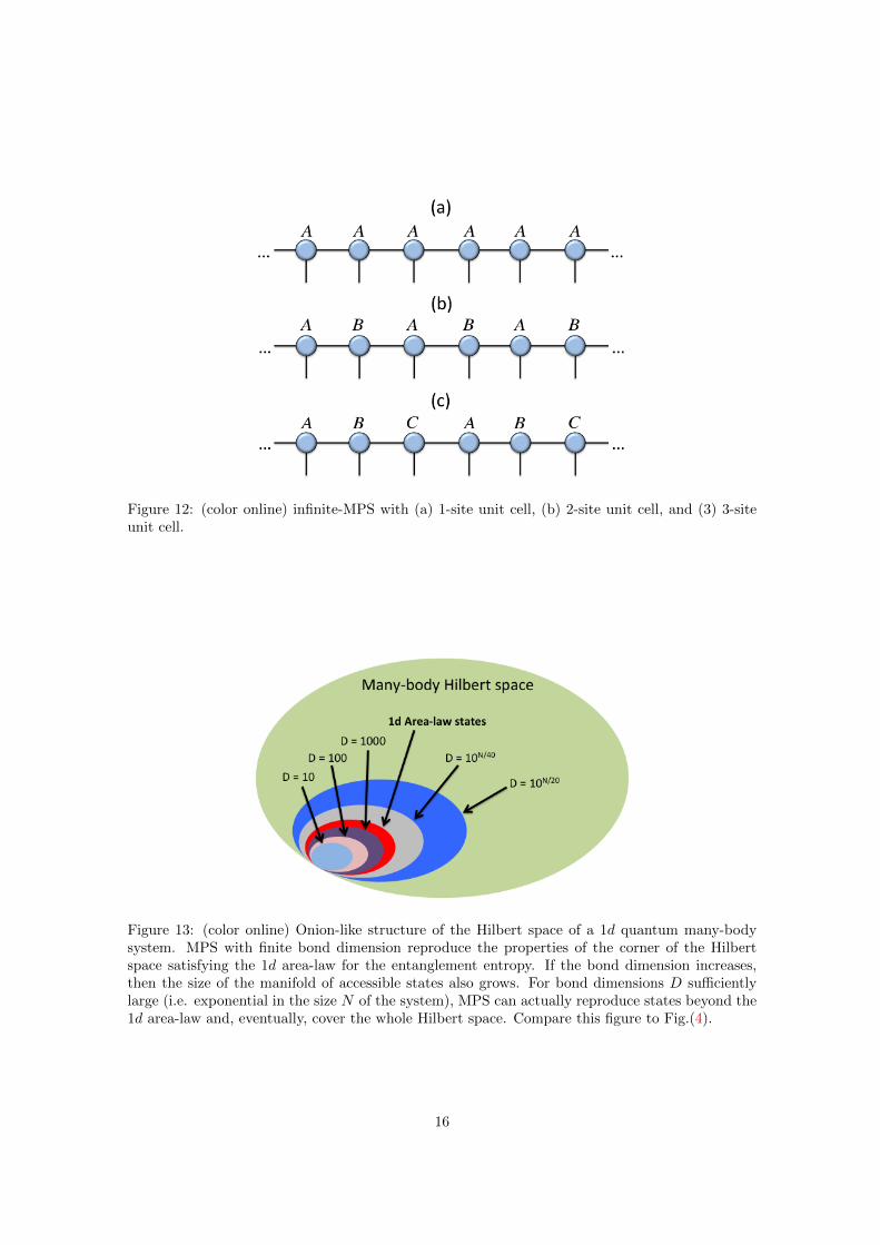
Figure 12: (color online) infinite-MPS with (a) 1-site unit cell, (b) 2-site unit cell, and (3) 3-siteunit cell.
Figure 13: (color online) Onion-like structure of the Hilbert space of a 1d quantum many-bodysystem. MPS with finite bond dimension reproduce the properties of the corner of the Hilbertspace satisfying the 1d area-law for the entanglement entropy. If the bond dimension increases,then the size of the manifold of accessible states also grows. For bond dimensions D sufficientlylarge (i.e. exponential in the size N of the system), MPS can actually reproduce states beyond the1d area-law and, eventually, cover the whole Hilbert space. Compare this figure to Fig.(4).
16

4) MPS are finitely-correlated.- The correlation functions of an MPS decay always expo-nentially with the separation distance. This means that the correlation length of these states isalways finite, and therefore MPS can not reproduce the properties of critical or scale-invariantsystems, where the correlation length is known to diverge [62]. We can understand this easily withthe following example: imagine that you are given a TI and infinite-size MPS defined in terms ofone tensor A, as in Fig.(12.a). The two-body correlator
C(r) ≡ 〈OiO′i+r〉 − 〈Oi〉〈O′i+r〉 (13)
of one-body operators Oi and O′i+r at sites i and i+ r can be represented diagrammatically as inFig.(14).
Figure 14: (color online) Diagrams for the two-body correlator C(r).
The zero-dimensional transfer matrix EI in Fig.(15.a) plays a key role in this calculation. Inparticular, we have that
(EI)r = (λ1)r
D2∑µ=1
(λiλ1
)r~RTi ~Li , (14)
where λi are the i = 1, 2, . . . , D2 eigenvalues of EI sorted in order of decreasing magnitude, and~Ri, ~Li their associated right- and left-eigenvectors. Assuming that the largest magnitude eigenvalueλ1 is non-degenerate, for r � 1 we have that
(EI)r ∼ (λ1)r
(~RT1 ~L1 +
(λ2
λ1
)r ω+1∑µ=2
~RTµ ~Lµ
), (15)
where ω is the degeneracy of λ2. Defining the matrices EO and EO′ as in Fig.(15.b), and usingthe above equation, it is easy to see that
〈OiO′i+r〉 ∼(~L1EO ~R
T1 )(~L1EO′ ~R
T1 )
λ21
+
(λ2
λ1
)r−1 ω+1∑µ=2
(~L1EO ~RTµ )(~LµEO′ ~R
T1 )
λ21
, (16)
which is expressed in terms of diagrams as in Fig.(16). In this equation, the first term is nothingbut 〈Oi〉〈O′i+r〉. Therefore, C(r) is given for large r by
C(r) ∼(λ2
λ1
)r−1 ω+1∑µ=2
(~L1EO ~RTµ )(~LµEO′ ~R
T1 )
λ21
(17)
17

Figure 15: (color online) (a) Transfer matrix EI; (b) matrix EO.
Figure 16: (color online) Diagrams for 〈OiO′i+r〉 for large separation distance r. The first partcorresponds to 〈Oi〉〈O′i+r〉.
so thatC(r) ∼ f(r)ae−r/ξ (18)
with a proportionality constant a = O(ω), f(r) a site-dependent phase = ±1 if O and O′ arehermitian, and correlation length ξ ≡ −1/ log |λ2/λ1|. Importantly, this type of exponential decayof two-point correlation functions for large r is the typical one in ground states of gapped non-critical 1d systems, which is just another indication that MPS are able to approximate well thistype of states.
5) Exact calculation of expectation values.- The exact calculation of the scalar productbetween two MPS for N sites can always be done exactly in a time O(NpD3). We explain thebasic idea for this calculation in Fig.(17). For an infinite system, the calculation can be done inO(pD3) using similar techniques as the ones explained above for the calculation of the two-pointcorrelator C(r) (namely, finding the dominant eigenvalue and dominant left/right eigenvectors ofthe transfer matrix EI). In general, expectation values of local observables such as correlationfunctions, energies, and local order parameters, can also be computed using the same kind oftensor manipulations.
6) Canonical form and the Schmidt decomposition.- Given a quantum state |Ψ〉 interms of an MPS with open boundary conditions, there is a choice of tensors called canonical formof the MPS [13, 14] which is extremely convenient. This is defined as follows: for a given MPS withopen boundary conditions (either for a finite or infinite system), we say that it is in its canonicalform [14] if, for each bond index α, the index corresponds to the labeling of Schmidt vectors in
18

Figure 17: (color online) Order of contractions for the scalar product of a finite MPS, startingfrom the left. The same strategy could be used for an infinite MPS, starting with some boundarycondition at infinity and iterating until convergence.
the Schmidt decomposition of |Ψ〉 across that index, i.e:
|Ψ〉 =
D∑α=1
λα|ΦLα〉 ⊗ |ΦRα 〉 . (19)
In the above equation, λα are Schmidt coefficients ordered into decreasing order (λ1 ≥ λ2 ≥ · · · ≥0), and the Schmidt vectors form orthonormal sets, that is, 〈ΦLα|ΦLα′〉 = 〈ΦRα |ΦRα′〉 = δαα′ .
For a finite system of N sites [13], the above condition corresponds to having the decompositionfor the coefficient of the wave-function
Ci1i2...iN = Γ[1]i1α1
λ[1]α1
Γ[2]i2α1α2
λ[2]α2
Γ[3]i3α2α3
λ[3]α3· · ·λ[N−1]
αN−1Γ[N ]iNαN−1
, (20)
where the Γ tensors correspond to changes of basis between the different Schmidt basis and thecomputational (spin) basis, and the vectors λ correspond to the Schmidt coefficients. In the case ofan infinite MPS with one-site traslation invariance [14], the canonical form corresponds to havingjust one tensor Γ and one vector λ describing the whole state. Regarding the Schmidt coefficients asthe entries of a diagonal matrix, the TN diagram for both the finite and infinite MPS in canonicalform are shown in Fig.(18).
Figure 18: (color online) (a) 4-site MPS in canonical form; (b) infinite MPS with 1-site unit cellin canonical form.
Let us now show a way to obtain the canonical form of an MPS |Ψ〉 for a finite system fromsuccessive Schmidt decompositions [13]. If we perform the Schmidt decomposition between the
19

site 1 and the remaining N − 1, we can write the state as
|Ψ〉 =
min(p,D)∑α1=1
λ[1]α1|τ [1]α1〉 ⊗ |τ [2···N ]
α1〉 , (21)
where λ[1]α1 are the Schmidt coefficients, and |τ [1]
α1 〉, |τ[2···N ]α1 〉 are the corresponding left and right
Schmidt vectors. If we rewrite the left Schmidt vector in terms of the local basis |i1〉 for site 1, thestate |Ψ〉 can then be written as
|Ψ〉 =
p∑i1=1
min(p,D)∑α1=1
Γ[1]i1α1
λ[1]α1|i1〉 ⊗ |τ [2···N ]
α1〉 , (22)
where Γ[1]i1α1 correspond to the change of basis |τ [1]
α1 〉 =∑i1
Γ[1]i1α1 |i1〉. Next, we expand each Schmidt
vector |τ [2···N ]α1 〉 as
|τ [2···n]α1
〉 =
p∑i2=1
|i2〉 ⊗ |ω[3···N ]α1i2
〉 . (23)
We now write the unnormalised quantum state |ω[3···N ]α1i2
〉 in terms of the at most p2 eigenvectors ofthe reduced density matrix for systems [3, . . . , N ], that is, in terms of the right Schmidt vectors
|τ [3···n]α2 〉 of the bipartition between subsystems [1, 2] and the rest, together with the corresponding
Schmidt coefficients λ[2]α2 :
|ω[3···N ]α1i2
〉 =
min(p2,D)∑α2=1
Γ[2]i2α1α2
λ[2]α2|τ [3···N ]α2
〉 . (24)
Replacing the last two expressions into Eq.(22) we get
|Ψ〉 =
p∑i1,i2=1
min(p,D)∑α1=1
min(p2,D)∑α2=1
(Γ[1]i1α1
λ[1]α1
Γ[2]i2α1α2
λ[2]α2
)|i1〉 ⊗ |i2〉 ⊗ |τ [3···N ]
α2〉 . (25)
Iterating the above procedure for all subsystems, we finally get
|Ψ〉 =∑{i}
∑{α}
(Γ[1]i1α1
λ[1]α1
Γ[2]i2α1α2
λ[2]α2. . . λ[N−1]
αN−1Γ[N ]iNαN−1
)|i1〉 ⊗ |i2〉 ⊗ · · · ⊗ |iN 〉 , (26)
where the sum over each index in {s} and {α} runs up to their respective allowed values. And thisis nothing but the representation that we mentioned in Eq.(20).
For an infinite MPS one can also compute the canonical form [14]. In this case one just needs tonotice that, in the canonical form, the bond indices of the MPS always correspond to orthonormalvectors to the left and right. Thus, finding the canonical form of an MPS is commonly referred toalso as orthonormalizing the indices of the MPS. For an infinite system defined by a single tensorA this canonical form can be found following the procedure indicated in the diagrams in Fig.(19).This can be summarized in three main steps:
(i) Find the dominant right eigenvector ~VR and the dominant left eigenvector ~VL of the transfer
matrices defined in Fig.(19.a). Regarding the bra/ket indices, ~VR and ~VL can also be understood ashermitian and positive matrices. Decompose these matrices as squares, VR = XX† and VL = Y †Y ,as shown in the figure.
(ii) Introduce I = (Y T )−1Y T and I = XX−1 in the bond indices of the MPS as shown inFig.(19.b). Next, calculate the singular value decomposition of the matrix product Y TλX = Uλ′V ,
20

Figure 19: (color online) Canonicalization of an infinite MPS with 1-site unit cell (see text).
where U and V are unitary matrices and λ′ are the singular values. It is easy to show that thesesingular values correspond to the Schmidt coefficients of the Schmidt decomposition of the MPS.
(iii) Arrange the remaining tensors into a new tensor Γ′, as shown in Fig.(19.c). The MPS isnow defined in terms of λ′ and Γ′.
The above procedure produces an infinite MPS such that all its bond indices correspond toorthonormal Schmidt basis, and is therefore in canonical form by construction5.
The canonical form of an MPS has a number of properties that make it very useful for MPScalculations. First, the eigenvalues of the reduced density matrices of different “left vs right”bipartitions are just the square of the Schmidt coefficients, which is very useful for calculations ofe.g. entanglement spectrums and entanglement entropies. Moreover, the calculation of expectationvalues of local operators simplifies a lot, see the diagrams in Fig.(20).
But most importantly, the canonical form provides a prescription for the truncation of the bondindices of an MPS in numerical simulations: just keep the largest D Schmidt coefficients at everybond at each simulation step. This truncation procedure is optimal for a finite system as long aswe keep the locality of the truncation (i.e. only the tensors involved in the truncated index aremodified), see e.g. Ref.[13]. This prescription for truncating the bond indices turns out to be reallyuseful, and is at the basis of the TEBD method and related algorithms for 1d systems.
5.1.2 Some examples
Let us now give four specific examples of non-trivial states that can be represented exactly byMPS:
1) GHZ state.- The GHZ state of N spins-1/2 is given by
|GHZ〉 =1√2
(|0〉⊗N + |1〉⊗N
), (27)
5Two comments are in order: first, here we do not consider the case in which the dominant eigenvalues of thetransfer matrices are degenerate. Second, this canonical form can also be achieved by running the iTEBD algorithmon an MPS with an identity time evolution until convergence [14]. Quite probably, the same result can be obtainedby running iDMRG [31] with identity Hamiltonian and alternating left and right sweeps until convergence.
21

Figure 20: (color online) Expectation value of a 1-site observable for an MPS in canonical form:(a) 5-site MPS and (b) infinite MPS with 1-site unit cell.
where |0〉 and |1〉 are e.g. the eigenstates of the Pauli σz operator (spin “up” and “down”) [63].This is a highly entangled quantum state of the N spins, which has some non-trivial entanglementproperties (e.g. it violates certain N -partite Bell inequalities). Still, this state can be representedexactly by a MPS with bond dimension D = 2 and periodic boundary conditions. The non-zerocoefficients in the tensor are shown in the diagram of Fig.(21).
Figure 21: (color online) Non-zero components for the MPS tensors of the GHZ state.
2) 1d cluster state.- Introduced by Raussendorf and Briegel [64], the cluster state in a 1dchain can be seen as the +1 eigenstate of a set of mutually commuting stabilizer operators {K [i]}defined as
K [i] ≡ σi−1z σixσ
i+1z , (28)
where the σiα are the usual spin-1/2 Pauli matrices with α ∈ {x, y, z} at lattice site i. Since(Ki)2 = I, for an infinite system this quantum state can be written (up to an overall normalizationconstant) as
|Ψ1dCL〉 =∏i
(I +K [i]
)2
|0〉⊗N→∞ . (29)
Each one of the terms(I +K [i]
)/2 is a projector that admits a TN representation with bond
dimension 2 as in Fig.(22.a). From here, it is easy to obtain an MPS description with bonddimension D = 4 for the 1d cluster state |Ψ1dCL〉, as shown in Fig.(22.b). The non-zero coefficientsof the MPS tensors follows easily from the corresponding TN contractions in the diagram.
22

Figure 22: (color online) MPS for the 1d cluster state: (a) tensor network decomposition of theoperator
(I +K [i]
)/2 and non-zero coefficients of the tensors; (b) construction of the infinite MPS
with 1-site unit cell.
Figure 23: (color online) MPS for the AKLT state: (a) spin-1/2 particles arranged in singlets|Φ〉 = 2−1/2(|0〉 ⊗ |1〉 − |1〉 ⊗ |0〉), and projected by pairs into the spin-1 subspace by projector P ;(b-c) non-zero components of the tensors for the infinite MPS with 1-site unit cell: (b) in termsof σ1 =
√2σ+, σ2 = −
√2σ− and σ3 = σz, with σ± = (σx ± σy)/2; (c) There is a gauge in which
these coefficients are given by the three spin-1/2 Pauli matrices σ1 = σx, σ2 = σy and σ3 = σz.
23

3) 1d AKLT model.- The state we consider now is the ground state of the 1d AKLT model[65]. This is a quantum spin chain of spin-1, that is given by the Hamiltonian
H =∑i
(~S[i]~S[i+1] +
1
3(~S[i]~S[i+1])2
), (30)
where ~S[i] is the vector of spin-1 operators at site i, and where again we assumed an infinite-sizesystem. This model was introduced by Affleck, Kennedy, Lieb and Tasaki in Ref.[65], and it wasthe first analytical example of a quantum spin chain supporting the so-called Haldane’s conjecture:it is a local spin-1 Hamiltonian with Heisenberg-like interactions and a non-vanishing spin gap inthe thermodynamic limit. What is also remarkable about this model is that its ground state isgiven exactly, and by construction, in terms of a MPS with bond dimension D = 2. This canbe understood in terms of a collection of spin-1/2 singlets, whose spins are paired and projectedinto spin-1 subspaces as indicated in Fig.(23.a). This, by construction, is an MPS with D = 2.Interestingly, there is a choice of tensors for the MPS (i.e. a gauge) such that these are given by thethree spin-1/2 Pauli matrices, which are the generators of the irreducible representation of SU(2)with 2×2 matrices (see Fig.(23.c)). We will not enter into details of why this representation for theMPS tensors is possible. For the curious reader, let us simply mention that this is a consequenceof the SU(2) symmetry of the Hamiltonian, which is inherited by the ground state, and which isalso reflected at the level of the individual tensors of the MPS.
4) Majumdar-Gosh model.- We now consider the ground state of the Majumdar-Goshmodel [66], which is a frustrated 1d spin chain defined by the Hamiltonian
H =∑i
(~S[i]~S[i+1] +
1
2~S[i]~S[i+2]
), (31)
where ~S[i] is the vector of spin-1/2 operators at site i. The ground state of this model is given bysinglets between nearest-neighbor spins, as shown in Fig.(24). Nevertheless, to impose translationalinvariance we need to consider the superposition between this state and its traslation by one latticesite. The resultant state can be written in compact notation with an MPS of bond dimensionD = 3,also as shown in Fig.(24).
Figure 24: (color online) MPS for the Majumdar-Gosh state: (a) the superposition of two dimerizedstates of singlets |Φ〉 in (a) can be written in terms of an infinite MPS with 1-site unit cell, withnon-zero coefficients as in (b).
24

5.2 Projected Entangled Pair States (PEPS)
The family of PEPS [16] is just the natural generalization of MPS to higher spatial dimensions.Here we shall only consider the 2d case. 2d PEPS are at the basis of several methods to simulate2d quantum lattice systems, e.g. PEPS [16] and infinite-PEPS [32] algorithms, as well as TensorRenormalization Group (TRG) [18], Second Renormalization Group (SRG) [29], Higher-OrderTensor Renormalization Group (HOTRG) [30], and methods based on Corner Transfer Matrices(CTM) and Corner Tensors [33, 67, 68]. In Secs.6-7 of these notes we will describe basic aspectsof some of these methods.
PEPS are TNs that correspond to a 2d array of tensors. For instance, for a 4×4 square lattice,we show the corresponding PEPS in Fig.(25), both with open and periodic boundary conditions.As such this generalization may look quite straightforward, yet we will see that the properties ofPEPS are remarkably different from those of MPS. Of course, one can also define PEPS for othertypes of 2d lattices e.g. honeycomb, triangular, kagome... yet, in these notes we mainly considerthe square lattice case. Moreover, and as expected, there are also two types of indices in a PEPS:physical indices, of dimension p, and bond indices, of dimension D.
Figure 25: (color online) 4 × 4 PEPS: (a) open boundary conditions, and (b) periodic boundaryconditions.
5.2.1 Some properties
We now sketch some of the basic properties of PEPS:
1) 2d Translational invariance and the thermodynamic limit.- As in the case of MPS,one is free to choose all the tensors in the PEPS to be different, which leads to a PEPS thatis not TI. Yet, it is again possible to impose TI and take the thermodynamic limit by choosinga fundamental unit cell that is repeated all over the (infinite) 2d lattice, see e.g. Fig.(26). Asexpected for higher-dimensional systems, TI needs to be imposed in all the spatial directions ofthe lattice.
2) PEPS are dense.- As was the case of MPS, PEPS is a dense family of states, meaningthat they can represent any quantum state of the many-body Hilbert space just by increasingthe value of the bond dimension D. As happens for MPS, the bond dimension D of a PEPSneeds to be exponentially large in the size of the system in order to cover the whole Hilbert space.Nevertheless, one expects D to be reasonably small and finite for low-energy states of interesting2d quantum models. In practice this is observed numerically [32], but there are also theoreticalarguments in favor of this property. For instance, it is well known that D = 2 is sufficient to
25

Figure 26: (color online) Infinite PEPS with (a) 1× 1 unit cell, (b) 2× 2 unit cell with 2 tensors,(c) 2× 2 unit cell with 4 tensors, and (d) 2× 3 unit cell with 6 tensors.
handle polynomially-decaying correlation functions (and hence critical states) [69], and that PEPScan also approximate with arbitrary accuracy thermal states of 2d local Hamiltonians [57]. In thiscase, a similar picture to the one in Fig.(13) would also apply adapted to the case of PEPS andthe 2d area-law.
3) 2d Area-law.- PEPS satisfy also the area-law scaling of the entanglement entropy. This wasshown already in the example of Fig.(10), but the validity is general. In practice, the entanglemententropy of a block of boundary L of a PEPS with bond dimension D is always S(L) = O(L logD).As discussed before, this property is satisfied by many interesting quantum states of quantum many-body systems, such as some ground states and low-energy excited states of local Hamiltonians.
4) PEPS can handle polynomially-decaying correlations.- A remarkable difference be-tween PEPS and MPS is that PEPS can handle two-point correlation functions that decay poly-nomially with the separation distance [69]. And this happens already for the smallest non-trivialbond dimension D = 2. This property is important, since correlation functions that decay poly-nomially (as opposed to exponentially) are characteristic of critical points, where the correlationlength is infinite and the system is scale invariant. Hence, the class of PEPS is suitable to describe,in principle, gapped phases as well as critical states of matter.
This property can be seen with the following example [69]: consider the unnormalized state
|Ψ(β)〉 = e−βH/2|+〉⊗N→∞ , (32)
26

with |+〉 = 2−1/2(|0〉+ |1〉), and H given by
H = −∑〈~r,~r′〉
σ[~r]z σ
[~r′]z . (33)
After some simple algebra it is easy to see that the norm of this quantum state is proportional tothe partition function of the 2d classical Ising model on a square lattice at inverse temperature β,i.e.:
〈Ψ(β)|Ψ(β)〉 ∝ Z(β) =∑{s}
e−βK({s}) , (34)
with K({s}) the classical Ising Hamiltonian,
K({s}) = −∑〈~r,~r′〉
s[~r]s[~r′] , (35)
where s[~r] = ±1 is a classical spin variable at lattice site ~r, and {s} is some configuration ofall the classical spins. It is also easy to see that the expectation values of local operators in|Ψ(β)〉 correspond to classical expectation values of local observables in the classical model. For
instance, the expectation value of σ[~r]z corresponds to the classical magnetization at site ~r at inverse
temperature β,
〈s[~r]〉β =〈Ψ(β)|σ[~r]
z |Ψ(β)〉〈Ψ(β)|Ψ(β)〉
=1
Z(β)
∑{s}
s[~r]e−βK({s}) . (36)
Also, the two-point correlation functions in the quantum state correspond to classical correlation
functions of the classical model. For instance, the correlation function for operators σ[~r]z and σ
[~r′]z
at sites ~r and ~r′ corresponds to the usual correlation function of the classical Ising variables,
〈s[~r]s[~r′]〉β =〈Ψ(β)|σ[~r]
z σ[~r′]z |Ψ(β)〉
〈Ψ(β)|Ψ(β)〉=
1
Z(β)
∑{s}
s[~r]s[~r′]e−βK({s}) . (37)
At the critical inverse temperature βc = (log(1+√
2))/2 it is well known that the correlation lengthof the system diverges, and the above correlation function decays polynomially for long separationdistances as
〈s[~r]s[~r′]〉βc≈ a
|~r − ~r′|1/4, (38)
for some constant a = O(1) and |~r − ~r′| � 1. The next step is to realize that, actually, thequantum state |Ψ(β)〉 is a 2d PEPS with bond dimension D = 2. This is shown in the tensornetwork diagrams in Fig.(27). Therefore, at the critical value β = βc, the resultant quantum state|Ψ(βc)〉 is an example of a 2d PEPS with finite bond dimension D = 2 and with polynomiallydecaying correlation functions (and hence infinite correlation length).This should be considered asa proof of principle about the possibility of having some criticality in a PEPS with finite bonddimension. As a remark, notice that this is totally different to the case of 1d MPS, where we sawbefore that two-point correlation functions always decay exponentially fast with the separationdistance.
Notice, though, that the criticality obtained in this PEPS is essentially classical, since we justcodified the partition function of the 2d classical Ising model as the squared norm of a 2d PEPS.Recalling the quantum-classical correspondence that a quantum d-dimensional lattice model isequivalent to some classical d+ 1-dimensional lattice model [70], one realizes that this criticality isactually the one from the 1d quantum Ising model, but “hidden” into a 2d PEPS with small D. Bygeneralizing this idea, we could actually think as well of e.g. “codifying” the quantum criticality ofa 2d quantum model into a 3d PEPS with small D. Yet, it is still unclear under which conditionsa 2d PEPS could handle this true 2d quantum criticality for small D as well.
27

Figure 27: (color online) PEPS for a (classical) thermal state: (a) tensor network decomposition
of the operator exp(−βσ[~r]z σ
[~r′]z /2) and non-zero coefficients of the tensors; (b) construction of the
infinite PEPS with 1-site unit cell.
5) Exact contraction is ]P-Hard: The exact calculation of the scalar product betweentwo PEPS is an exponentially hard problem. This means that for two arbitrary PEPS of Nsites, it will always take a time O(exp(N)), no matter the order in which we try to contract thedifferent tensors. This statement can be done mathematically precise. From the point of viewof computational complexity, the calculation of the scalar product of two PEPS is a problemin the complexity class ]P-Hard [71]. We shall not enter into detailed definitions of complexityclasses here, yet let us explain in plain terms what this means. The class ]P-Hard is the classof problems related to counting the number of solutions to NP-Complete problems. Also, theclass NP-Complete is commonly understood as a class of very difficult problems in computationalcomplexity6, and it is widely believed that there is no classical (and possibly quantum) algorithmthat can solve the problems in this class using polynomial resources in the size of the input. Asimilar statement is also true for the class ]P-Hard. Therefore, unlike for 1d MPS, computing exactscalar products of arbitrary 2d PEPS is, in principle, inefficient.
However, and as we will see in Sec.6, it is possible in practice to approximate these expectationvalues using clever numerical methods. Moreover, recent promising results in the study of entan-glement spectra seem to indicate that these approximate calculations can be done with a verylarge accuracy (possibly even exponential), at least for 2d PEPS corresponding to ground statesof gapped, local 2d Hamiltonians [73].
6) No exact canonical form.- Unlike for MPS with open boundary conditions, there isno canonical form of a PEPS, in the sense that it is not possible to choose orthonornal basissimultaneously for all the bond indices. In fact, this happens already for MPS with periodicboundary conditions or, more generally, as long as we have a loop in the TN. Loosely speaking, aloop in the TN means that we can not formally split the network into left and right pieces by justcutting one index, so that a Schmidt decomposition between left and right does not make sense. Inpractice this means that we can not define orthonormal basis (i.e. Schmidt basis) to the left and
6The interested reader can take a look at e.g. Ref.[72].
28

right of a given index, and hence we can not define a canonical form in this sense (see Fig.(28)).
Figure 28: (color online) By “cutting” a link in a TN, one can define left and right pieces if thereare no other connecting indices between the two pieces (a), whereas this is not possible if otherconnecting indices exist (b).
Nevertheless, it is observed numerically that for non-critical PEPS it is usually possible to finda quasi-canonical form, which leads to approximate numerical methods for finding ground states(a variation of the so-called “simple update” approach [74]). We refer the interested reader toRef.[75] for more details about this.
5.2.2 Some examples
In what follows we provide some examples of interesting quantum states for 2d lattices that canbe expressed exactly using the PEPS formalism. These are the following:
1) 2d Cluster State.- The cluster state in a 2d square lattice [64] is highly-entangled quan-tum state that can be used as a resource for performing universal measurement-based quantumcomputation. This quantum state is the +1 eigenstate of a set of mutually commuting stabilizeroperators {K [~r]} defined as
K [~r] ≡ σ[~r]x
⊗~p∈Γ(~r)
σ[~p]z , (39)
where Γ(~r) denotes the four nearest-neighbor spins of lattice site ~r and the σ[~r]α are the usual
spin-1/2 Pauli matrices with α ∈ {x, y, z} at lattice site ~r. For the infinite square lattice, thesestabilizers are five-body operators. Noticing that (K [~r])2 = I, this quantum state can be written(up to an overall normalization constant) as
|Ψ2dCL〉 =∏~r
(I +K [~r]
)2
|0〉⊗N→∞ . (40)
Each one of the terms(I +K [~r]
)/2 is a projector that admits a TN representation as in Fig.(29).
From here, it is easy to obtain a TN description for the 2d cluster state |Ψ2dCL〉 in terms of a 2dPEPS with bond dimension D = 4, as shown in Fig.(29). In the figure we also give the value ofthe non-zero coefficients of the PEPS tensors.
2) Toric Code model.- The Toric Code, introduced by Kitaev [76], is a model of spins-1/2on the links of a 2d square lattice. The Hamiltonian can be written as
H = −Ja∑s
As − Jb∑p
Bp , (41)
29

Figure 29: (color online) PEPS for the 2d cluster state: (a) tensor network decomposition of theoperator
(I +K [~r]
)/2 and non-zero coefficients of the tensors; (b) construction of the infinite PEPS
with 1-site unit cell.
where As and Bp are star and plaquette operators such that
As =∏~r∈s
σ[~r]x , Bp =
∏~r∈p
σ[~r]z . (42)
In other words, As is the product of σx operators for the spins around a star, and Bp is the productof σz operators for the spins around a plaquette. Here we will be considering the case of an infinite2d square lattice.
The Toric Code is of relevance for a variety of reasons. First, it can be seen as the Hamiltonianof a Z2 lattice gauge theory with a “soft” gauge constraint [77] (i.e. if we send either Ja or Jbto infinity, then we recover the low-energy sector of the lattice gauge theory). But also, it isimportant because it is the simplest known model such that its ground state displays the so-called“topological order”, which is a kind of order in many-body wave-functions related to a pattern oflong-range entanglement that prevades over the whole quantum state (here we shall not discusstopological order in detail; the interested reader can have a look at the vast literature on this topic,e.g. Ref.[4]). Furthermore, the Toric Code is important in the field of quantum computation, sinceone could use its degenerate ground state subspace on a torus geometry to define a topologicallyprotected qubit that is inherently robust to local noise [76].
An interesting feature about the Toric Code is that, again, it can be understood as a sumof mutually commuting stabilizer operators. This time the stabilizers are the set of star andplaquette operators {As} and {Bp}. As for the cluster state, it is easy to check that the square ofthe stabilizer operators equals the identity (A2
s = B2p = I ∀s, p). The ground state of the system
is the +1 eigenstate of all these stabilizer operators. For an infinite 2d square lattice this groundstate is unique, and can be written (up to a normalization constant) as
|ΨTC〉 =∏s
(I +As)
2
∏p
(I +Bp)
2|0〉⊗N→∞ =
∏s
(I +As)
2|0〉⊗N→∞ , (43)
where the last equality follows from the fact that the state |0〉⊗N→∞ is already a +1 eigenstateof the operators Bp for any plaquette p. The above state can be written easily as a PEPS withbond dimension D = 2 [69]. For this, notice that each one of the terms (I + As)/2 for any star sadmits the TN representation from Fig.(30.a). From here, a PEPS representation with a 2-site unitcell as in Fig.(26.b) follows easily, see Fig.(30.b). As we can see with this example, a PEPS with
30

Figure 30: (color online) PEPS for the Toric Code: (a) tensor network decomposition of operator(I +As) /2 and non-zero coefficients of the tensors; (b) construction of the infinite PEPS with 2×2unit cell and 2 tensors.
the smallest non-trivial bond dimension D = 2 can already handle topologically ordered states ofmatter.
3) 2d Resonating Valence Bond State.- The 2d Resonating Valence Bond (RVB) state[78], is a quantum state proposed by Anderson in 1987 in the context of trying to explain themechanisms behind high-Tc superconductivity. For our purposes this state corresponds to theequal superposition of all possible nearest-neighbor dimer coverings of a lattice, where each dimeris a SU(2) singlet,
|Φ〉 =1√2
(|0〉 ⊗ |1〉 − |1〉 ⊗ |0〉) , (44)
which is a maximally-entangled state of two qubits (also known as EPR pair, or Bell state). Forthe 2d square lattice this is represented in Fig.(31.a). This state is also important since it is thearquetypical example of a quantum spin liquid: a quantum state of matter that does not breakany symmetry (neither translational symmetry, nor SU(2)). Importantly, this RVB state can alsobe written as a PEPS with bond dimension D = 3. The non-zero coefficients of the tensors aregiven in Fig.(31.b).
Figure 31: (color online) A 2d Resonating Valence Bond state built from nearest-neighbor singlets(a) can be written as an infinite PEPS with 1-site unit cell, with non-zero coefficients of the tensorsas in (b).
31

4) 2d AKLT model.- The 2d AKLT model on a honeycomb lattice [65, 79] is given by theHamiltonian
H =∑〈~r,~r′〉
(~S[~r]~S[~r′] +
116
243
(~S[~r]~S[~r′]
)2
+16
243
(~S[~r]~S[~r′]
)3), (45)
where ~S[~r] is the vector of spin-3/2 operators at site ~r, and the sum is over nearest-neighbor spins.As explained in Ref.[65, 79], this model can be seen as a generalization of the 1d AKLT modelin Eq.(30) to two dimensions. The ground state can be understood in terms of a set of spin-1/2singlets, which are brought together into groups of 3 at every vertex of the honeycomb lattice, andprojected into their symmetric subspace (i.e. spin-3/2), see Fig.(32). By construction, this is a 2dPEPS with bond dimension D = 2.
Figure 32: (color online) PEPS for the 2d AKLT state on the honeycomb lattice. Spin-1/2 particlesarranged in singlets |Φ〉 = 2−1/2(|0〉 ⊗ |1〉 − |1〉 ⊗ |0〉), and projected in trios using projectorP = (|1〉〈0| ⊗ 〈0| ⊗ 〈0| + |2〉〈1| ⊗ 〈1| ⊗ 〈1| + |3〉〈W | + |4〉〈W |), with |W 〉 = 3−1/2(|0〉 ⊗ |0〉 ⊗ |1〉 +|0〉 ⊗ |1〉 ⊗ |0〉+ |1〉 ⊗ |0〉 ⊗ |0〉) and |W 〉 = 3−1/2(|1〉 ⊗ |1〉 ⊗ |0〉+ |1〉 ⊗ |0〉 ⊗ |1〉+ |0〉 ⊗ |1〉 ⊗ |1〉).
6 Extracting information: computing expectation values
An important problem for TN is how to extract information from them. This is usually achievedby computing expectation values of local observables. It turns out that such expectation valuescan be computed efficiently, either exactly (for MPS) or approximately (for PEPS). This is veryimportant, since otherwise it would not make any sense to have an efficient representation of aquantum state: we also need to be able to extract information from it!
In what follows we explain how expectation values can be extracted efficiently from MPS andPEPS, both for finite and infinite systems. In fact, in the case of MPS with open boundaryconditions a lot of the essential information was already introduced in Sec.4, when talking aboutthe exponential decay of two-point correlation functions and the exact calculation of norms.
We will see that the calculation of expectation values follows many times a dimensional reduc-tion strategy. More precisely, the 1d problem for an MPS is reducible to a 0d problem, and thiscan be solved exactly. Also, the 2d problem for a PEPS is reducible to a 1d problem that can besolved approximately using MPS techniques. This MPS problem, in turn, is itself reducible to a0d problem that is again exactly solvable. Such a dimensional reduction strategy is nothing butan implementation, in terms of TN calculations, of the ideas of the holographic principle [1].
6.1 Expectation values from MPS
Expectation values of local operators can be computed exactly for an MPS without the need forfurther approximations. In the case of open boundary conditions, this is achieved for finite and
32

infinite systems using the techniques that we already introduced in Fig.(17). As explained inSec.5, all those manipulations can be done easily in O(NpD3) time for finite systems, and O(pD3)for infinite [62]. The trick for infinite systems is to contract from the left and from the right asindicated in the figure, assuming some boundary condition placed at infinity. In practice, sucha contraction is equivalent to finding the dominant left and right eigenvectors of the 0d transfermatrix from Fig.(15). Let us remind that these calculations are very much simplified if the MPSis in canonical form, see Fig.(20).
If the MPS has periodic boundary conditions [11], then the TN contractions for expectationvalues are similar to the ones in Fig.(33). This time the calculation can be done in O(NpD5) time.As expected, the calculation for periodic boundary conditions is less efficient than the one for openboundary conditions, since one needs to carry more tensor indices at each calculation step.
Figure 33: (color online) order of contractions for an MPS with periodic boundary conditions
6.2 Expectation values from PEPS
Unlike for MPS, expectation values for PEPS need to be computed using approximations. Here weexplain some techniques to do this for the case of finite systems with open boundary conditions,as well as for infinite systems. The methods explained here are by far not the only ones (see e.g.Ref.[67] and Ref.[30] for some alternatives), yet they are quite representative, and constitute alsothe first step towards understanding many of the calculations that are involved in the numericalalgorithms for finite and infinite-PEPS.
Let us introduce a couple of definitions before proceeding any further. We call the environmentE [~r] of a site ~r the TN consisting of all the tensors in the original TN, except those at site ~r,see Fig.(34). Unlike for MPS, environments for sites of a PEPS can not be computed exactly.Therefore, we call effective environment G[~r] of a site ~r the approximation of the contraction of theexact environment of site ~r by using some “truncation” criteria in the relevant degrees of freedom.In what follows we shall be more explicit with what we mean by this “truncation”.
33

Figure 34: (color online) The environment of a site corresponds to the contraction of the wholetensor network except for the tensors at that site.
6.2.1 Finite systems
Consider the expectation value of a local one-site observable for a finite PEPS [16]. The TNthat needs to be contracted corresponds to the one in the diagram in Fig.(35.a) which can beunderstood in terms of a 2d lattice of reduced tensors as in Fig.(35.b). As explained earlier, theexact contraction of such a TN is a ]P-Hard problem, and therefore must be approximated.
Figure 35: (color online) (a) Expectation value of a 1-site observable for a 4 × 4 PEPS; (b)Contraction of the 4× 4 lattice of reduced tensors. We use thick lines to indicate “double” indicesranging from 1 to D2.
The way to approximate this calculation is by reducing the original 2d problem to a seriesof 1d problems that we can solve using MPS methods such as DMRG or TEBD. Let us do thisas follows: first, consider the upper-row boundary of the system (in this case we have a squarelattice). The tensors within this row can be understood as forming an MPS if the physical indices
34

Figure 36: (color online) Strategy to contract the lattice of reduced tensors for a finite PEPS.
are contracted at each site, see Fig.(36.a). Next, the contraction of this MPS with the next row oftensors is equivalent to the action of a Matrix Product Operator (MPO) on the MPS, see Fig.(36.b).This is, by construction, an MPS of higher bond dimension than the original (actually of bonddimension D4). Therefore, in order to maintain the bond dimension under control, we approximatethe resultant MPS by another MPS of lower bond dimension which we call χ, see Fig.(36.c). Thisapproximation can be done using e.g. DMRG or TEBD methods. We can proceed in this way inorder to add each one of the rows of the 2d lattice, and of course we can do the same but startingfrom the lower boundary. Proceeding in this way, both from up and down, we end up eventuallyin the contraction of the 1d TN shown in Fig.(36.d). But remarkably, what is now left is a 1dproblem! Therefore the remaining contractions can be computed exactly by reducing everythingto a 0d problem as explained in the previous section, i.e. we start contracting the tensors fromthe left, and then from the right, until we end up in the TN of Fig.(36.e). The final expectationvalue just follows from this contraction, dividing by the corresponding norm of the state (sameTN but without the observable operator). Overall, this procedure has a computational cost ofO(Np2χ2D6) in time.
In case you did not notice, what we just computed in the above procedure was an effectiveenvironment for the site where we placed the observable. This is not exclusive of this calculation:all the methods to compute expectation values of 2d systems are based on techniques to computeeffective environments of different sites. And not only that: some of the minimization techniquesfor 2d PEPS that will be discussed in the next section rely also heavily on the accurate calculationof effective environments.
35
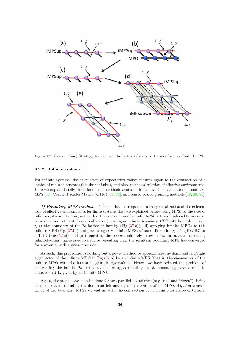
Figure 37: (color online) Strategy to contract the lattice of reduced tensors for an infinite PEPS.
6.2.2 Infinite systems
For infinite systems, the calculation of expectation values reduces again to the contraction of alattice of reduced tensors (this time infinite), and also, to the calculation of effective environments.Here we explain briefly three families of methods available to achieve this calculation: boundary-MPS [32], Corner Transfer Matrix (CTM) [67, 33], and tensor coarse-graining methods [18, 29, 30].
1) Boundary MPS methods.- This method corresponds to the generalization of the calcula-tion of effective environments for finite systems that we explained before using MPS, to the case ofinfinite systems. For this, notice that the contraction of an infinite 2d lattice of reduced tensors canbe understood, at least theoretically, as (i) placing an infinite boundary MPS with bond dimensionχ at the boundary of the 2d lattice at infinity (Fig.(37.a)), (ii) applying infinite MPOs to thisinfinite MPS (Fig.(37.b)) and producing new infinite MPSs of bond dimension χ using iDMRG oriTEBD (Fig.(37.c)), and (iii) repeating the process infinitely-many times. In practice, repeatinginfinitely-many times is equivalent to repeating until the resultant boundary MPS has convergedfor a given χ with a given precision.
As such, this procedure, is nothing but a power method to approximate the dominant left/righteigenvector of the infinite MPO in Fig.(37.b) by an infinite MPS (that is, the eigenvector of theinfinite MPO with the largest magnitude eigenvalue). Hence, we have reduced the problem ofcontracting the infinite 2d lattice to that of approximating the dominant eigenvector of a 1dtransfer matrix given by an infinite MPO.
Again, the steps above can be done for two parallel boundaries (say “up” and “down”), beingthus equivalent to finding the dominant left and right eigenvectors of the MPO. So, after conver-gence of the boundary MPSs we end up with the contraction of an infinite 1d stripe of tensors.
36

This remaining contraction can be done exactly, just by reducing the problem to that of findingthe dominant left and right eigenvectors of the 0d transfer matrix EI in Fig.(37.d). The finalcontraction produces the effective environment given in Fig.(37.e).
A comment is now in order. Notice that in this procedure we decided to place our infiniteboundary MPS at the “up” and “down” boundaries, hence using horizontal MPSs. But this choiceis not unique. For instance, we could have chosen equally well the “left” and “right” boundaries,hence using vertical MPSs. What is more, we could have chosen to work with diagonal boundaryMPS such as the ones in Fig.(38). In such a case, the infinite MPO as well as the relevant 0dtransfer matrix EI have a different construction (see the figure). While the final result does notdepend too much on how we choose to place the boundary MPS, the computational cost does. Inparticular, the horizontal (or vertical) MPS method has a computational cost of O(χ3D6 +pχ2D8),whereas the diagonal MPS method has a slightly lower computational cost of O(χ3D4 + pχ2D6)[32].
Figure 38: (color online) 1-dimensional problem obtained when contracting the infinite 2d latticeof reduced tensors using diagonal boundary MPS.
2) CTM methods.- CTM methods are a different way of computing effective environmentsfor 2d infinite PEPS. To understand this, let us consider the environment E [~r] of lattice site ~r.Another way of understanding this environment is to think that it comes from the contractions ofthe four corners of tensors, together with two half-row and two half-column 1d transfer matrices,as shown in Fig.(39).
The contraction of the TN corresponding to all the tensors in a corner is a well-known objectcalled corner transfer matrix, and is known to have very nice spectral properties (see e.g. the worksby Baxter in Ref.[80]). The aim of CTM contraction methods is to find an approximate, renor-malized version of the exact CTMs, half-row and half-column transfer matrices. This can be donenumerically in several ways. One possibility is to use the Corner Transfer Matrix RenormalizationGroup (CTMRG) developed by Nishino et al [67]. Here we explain a variation of this method,called directional CTM approach [33], which is more efficient and essentially as accurate (in mostcases) as the original CTMRG method.
In the directional CTM approach, the tensors are updated according to four directional moves,to the left, right, up and down, which are iterated until the environment converges. To be morespecific, we start from an effective environment G[~r] = {C1, T1, C2, T2, C3, T3, C4, T4}. Then, amove to e.g. the left is implemented by the following three steps:
(1) Insertion: starting from the effective environment G[~r] in Fig.(40.a), insert a new column
37

Figure 39: (color online) General strategy of Corner Transfer Matrix methods. The problem isreduced to contracting four CTMs, two half-row and two half-column transfer matrices.
Figure 40: (color online) Different steps in the directional CTM approach (see text).
as in Fig.(40.b).
(2) Absorption: contract tensors C1 and T1, tensors C4 and T3, and also tensors T4 and the
reduced PEPS tensor as indicated in Fig.(40.b). As a result, obtain two CTMs C1 and C4, and a
half-row transfer matrix T4, see Fig.(40.c).
(3) Renormalization: compute isommetry Z as in Fig.(41.a). Truncate it by keeping at most
χ values of the right index corresponding to the largest singular values DZ in the singular valuedecomposition, thus getting the truncated isommetry of Z. Finally, find two new CTMs C ′1 =
Z†C1, C ′4 = C4Z and a new half-row transfer matrix T ′4 as indicated in Fig.(41.b).
After these steps the new effective environment G′[~r] of a site in the lattice is given by thetensors G′[~r] = {C ′1, T1, C2, T2, C3, T3, C
′4, T
′4}, see Fig.(40.d). Also, the effective size of the system
increases by one column. The whole method continues by iterating this procedure in the differentdirections until convergence (of e.g. the singular values of the different CTMs). On the whole,the asymptotic computational cost in time of the directional CTM approach is O(χ3D6). Several
38
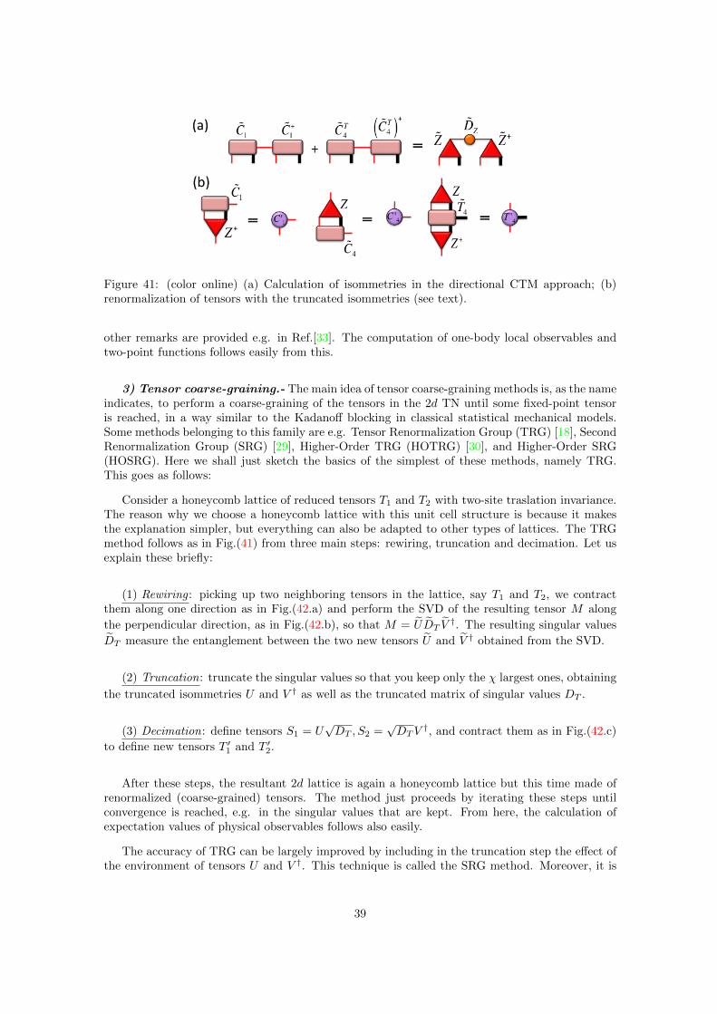
Figure 41: (color online) (a) Calculation of isommetries in the directional CTM approach; (b)renormalization of tensors with the truncated isommetries (see text).
other remarks are provided e.g. in Ref.[33]. The computation of one-body local observables andtwo-point functions follows easily from this.
3) Tensor coarse-graining.- The main idea of tensor coarse-graining methods is, as the nameindicates, to perform a coarse-graining of the tensors in the 2d TN until some fixed-point tensoris reached, in a way similar to the Kadanoff blocking in classical statistical mechanical models.Some methods belonging to this family are e.g. Tensor Renormalization Group (TRG) [18], SecondRenormalization Group (SRG) [29], Higher-Order TRG (HOTRG) [30], and Higher-Order SRG(HOSRG). Here we shall just sketch the basics of the simplest of these methods, namely TRG.This goes as follows:
Consider a honeycomb lattice of reduced tensors T1 and T2 with two-site traslation invariance.The reason why we choose a honeycomb lattice with this unit cell structure is because it makesthe explanation simpler, but everything can also be adapted to other types of lattices. The TRGmethod follows as in Fig.(41) from three main steps: rewiring, truncation and decimation. Let usexplain these briefly:
(1) Rewiring : picking up two neighboring tensors in the lattice, say T1 and T2, we contractthem along one direction as in Fig.(42.a) and perform the SVD of the resulting tensor M along
the perpendicular direction, as in Fig.(42.b), so that M = UDT V†. The resulting singular values
DT measure the entanglement between the two new tensors U and V † obtained from the SVD.
(2) Truncation: truncate the singular values so that you keep only the χ largest ones, obtaining
the truncated isommetries U and V † as well as the truncated matrix of singular values DT .
(3) Decimation: define tensors S1 = U√DT , S2 =
√DTV
†, and contract them as in Fig.(42.c)
to define new tensors T ′1 and T ′2.
After these steps, the resultant 2d lattice is again a honeycomb lattice but this time made ofrenormalized (coarse-grained) tensors. The method just proceeds by iterating these steps untilconvergence is reached, e.g. in the singular values that are kept. From here, the calculation ofexpectation values of physical observables follows also easily.
The accuracy of TRG can be largely improved by including in the truncation step the effect ofthe environment of tensors U and V †. This technique is called the SRG method. Moreover, it is
39

Figure 42: (color online) Different steps in the TRG method: (a) rewiring and SVD, (b) calculationof S1 and S2 and (c) decimation.
possible to improve the accuracy of both TRG and SRG by using the so-called Higher-Order SVD(or Tucker decomposition), which gives rise to the HOTRG and HOSRG methods. These shall notbe explained here, and the interested reader is referred to Refs.[18, 29, 30] for more information.
7 Determining the tensors: finding ground states
Independently of their analytical properties, MPS and PEPS are very useful because they can beused as numerical ansatzs for approximating interesting quantum many-body wave-functions, suchas ground states and low-energy excitations of local Hamiltonians. As we explained before, this isa very good idea since TNs are the states that target the relevant corner of the many-body Hilbertspace. To put it in other words: MPS and PEPS have in their built-in structure the area-lawfor the entanglement entropy, and therefore the correct entanglement behavior for many groundstates of gapped local systems (albeit with some exceptions at criticality [54, 55, 56]). Generallyspeaking, it is also known that MPS and PEPS approximate well the finite-temperature propertiesof gapped local Hamiltonians [57]. It is not surprising, thus, that MPS and PEPS turn out to bevery valuable ansatze when it comes to numerics.
However, there is still a basic question that needs to be addressed: how do we fill in thecoefficients of the tensors of MPS and PEPS? The answer is not unique: this can be done indifferent ways depending on the type of system (finite or infinite, 1d or 2d...) and the type of statethat is targeted (ground state, excitation, time-evolved state...). Explaining in detail all thesedifferent scenarios is far beyond the reach of this paper. Instead, here we explain the basic ideabehind the two most widely-used families of methods to find ground states with TNs, namely:variational optimization, and imaginary time evolution. This should be a good starting point forthe reader interested in learning the details of other techniques.
40

7.1 Variational optimization
Given a Hamiltonian H, the variational principle states that for a given quantum state |Ψ〉 it willalways be the case that
〈Ψ|H|Ψ〉〈Ψ|Ψ〉
≥ E0 , (46)
with E0 the lowest eigenvalue of H (i.e. the ground state energy). Therefore, if |Ψ〉 is a TNbelonging to some family of states like MPS or PEPS with a fixed bond dimension D, we canalways approach the ground state energy from above by minimizing this expectation value overthe relevant family, i.e.
min|Ψ〉∈family
(〈Ψ|H|Ψ〉 − λ〈Ψ|Ψ〉) , (47)
where by “family” we mean either MPS, or PEPS, or any other family of TN state with bonddimension D, and where λ is a Lagrange multiplier that introduces the constraint that |Ψ〉 musthave norm one.
Ideally, the above minimization should be done simultaneously over all the free parameters ofthe TN state, hence over all the coefficients of all the tensors for all sites. However this is normallyquite difficult to implement and not particularly efficient. Instead of this, the strategy is to proceedtensor by tensor. This is, to minimize with respect to one tensor while keeping the others fixed,then move to another tensor and repeat the minimization, and so on. In practice one sweeps overall the tensors several times until the desired convergence in expectation values is attained.
The way to minimize with respect to one tensor works as follows: imagine that we fix all thetensors in the TN except one of them which we call A. The coefficients of A are now our variationalparameters. The minimization is thus written as
minA
(〈Ψ|H|Ψ〉 − λ〈Ψ|Ψ〉) = minA
(~A†Heff ~A− λ ~A†N ~A
). (48)
In the above equation, ~A is just the tensor A but with all its coefficients arranged as a vector (seeFig.(43.a)), Heff is an effective Hamiltonian, and N is a normalization matrix. In practice, Heffand N correspond respectively to the TNs for 〈Ψ|H|Ψ〉 and 〈Ψ|Ψ〉 but without tensors A and A∗.That is, the environment of tensors A and A∗ in the two TNs, but written in matrix form (seeFig.(43.b)). Now, this minimization can be done as
∂
∂ ~A†
(~A†Heff ~A− λ ~A†N ~A
)= 0 , (49)
which leads to the generalized eigenvalue problem
Heff ~A = λN ~A . (50)
Once Heff and N are known this generalized eigenvalue problem can be solved numerically byusing standard linear algebra packages. And to calculate both Heff and N one must use thetools explained in the previous section to compute expectation values of physical observables and(effective) environments in a TN. In practice, this means that both Heff and N can be com-puted efficiently and exactly for an MPS, whereas for a PEPS this calculation is also efficient butapproximate.
A few remarks are in order. First, if we perform this optimization for an MPS with open bound-ary conditions, then what we recover is nothing but the famous Density Matrix RenormalizationGroup algorithm (DMRG) in the language of MPS [9, 10, 62]. This is particularly appealing, sinceusing this MPS picture is also now quite clear how to extend the method to periodic boundaryconditions [11]. Second, this variational technique has also been applied successfully for infinite
41

Figure 43: (color online) (a) A tensor can be transformed into a vector by moving and groupingits indices; (b) procedure to get the normalization matrix N .
MPS [31]. Not only that, but the method has also been applied successfully for e.g. finite PEPS[16], as well as other TNs such as TTNs [26] and the MERA [21]. Third, there are stability issuesin the algorithm depending on the behavior of the normalization matrix N . We postpone thediscussion about this point to Sec.(7.3).
7.2 Imaginary time evolution
The imaginary time evolution technique proceeds by evolving some initial state in imaginary timewith the Hamiltonian of interest. For very long times the resultant quantum state tends to be inthe ground state |E0〉, namely
|E0〉 = limτ→∞
e−τH |Ψ(0)〉√|〈Ψ(τ)|Ψ(τ)〉|
|Ψ(τ)〉 = e−τH |Ψ(0)〉 , (51)
for some initial quantum state |Ψ(0)〉 that has non-zero overlap with the ground state, and whereτ is the imaginary time.
The idea now is to find a way to implement such an evolution on the family of relevant TNstates, say e.g. MPS or PEPS, for a given quantum Hamiltonian. A way to achieve this is to splitthe time-evolution operator into small imaginary-time steps,
e−τH =(e−δτH
)m, (52)
where m = τ/δτ � 1. Next, let us assume for the sake of simplicity that the Hamiltonian is thesum of two-body nearest-neighbor terms, i.e.
H =∑〈ij〉
hi,j , (53)
42

where sites i and j are nearest neighbors in the lattice7. With this in mind, we can make theapproximation to first order in δτ
e−δτH =∏〈i,j〉
e−δτhij +O(δτ2) . (54)
The above is the so-called first-order Suzuki-Trotter expansion [81]. Further orders in this approxi-mation can also be considered if necessary if one wishes to reduce the associated error. Each of theterms in the multiplication above is also called a two-body gate, in a notation that is reminiscentfrom that used in the language of quantum circuits. This is, the two-body gate gij between sites iand j is given by
gij ≡ e−δτhij . (55)
As such, all the above equations mean that the imaginary-time evolution operator can be approx-imated by m � 1 repetitions of the operator U(δτ) ≡
∏〈i,j〉 gij . This simplifies a lot the original
problem, but still, one needs to know how to apply this operator on a given TN state. Luckilyenough there are many ways of achieving this, see e.g. the TN diagrams for MPSs from Fig.(44).
Figure 44: (color online) Different ways to apply the time evolution operator U(δτ) to an MPS:(a) parallel, (b) sequential, and (c) Matrix Product Operator.
Once the above points are clear, one must proceed according to the following strategy:
(1) Infinitesimal evolution: apply operator U(δτ) on a given TN state |Ψ〉 (e.g. MPS or PEPS)
with bond dimension D, obtaining a new TN state |Ψ〉 = U(δτ)|Ψ〉 with bond dimension D′ ≥ D.
(2) Truncation: approximate |Ψ〉 by a new TN state |Ψ′〉 back with bond dimension D.
The above two steps are very general, and there are many ways of implementing them dependingon (i) the dimensionality of the system, and (ii) the accuracy and efficiency that is desired. Asexpected, more accurate algorithms have a larger computational cost thus being less efficient,while less accurate algorithms, while being more efficient, may produce incorrect results if theentanglement in the system is large8. Just as an example, step (1) above can be implemented for1d systems as in Fig.(45) (the extension to 2d is straightforward). Furthermore, step (2) can beimplemented by e.g. minimizing the squared distance error
err =∣∣∣∣∣∣|Ψ′〉 − |Ψ〉∣∣∣∣∣∣2 . (56)
7Other types of interactions could also be considered easily.8This is specially true in the vicinity of a quantum critical point.
43
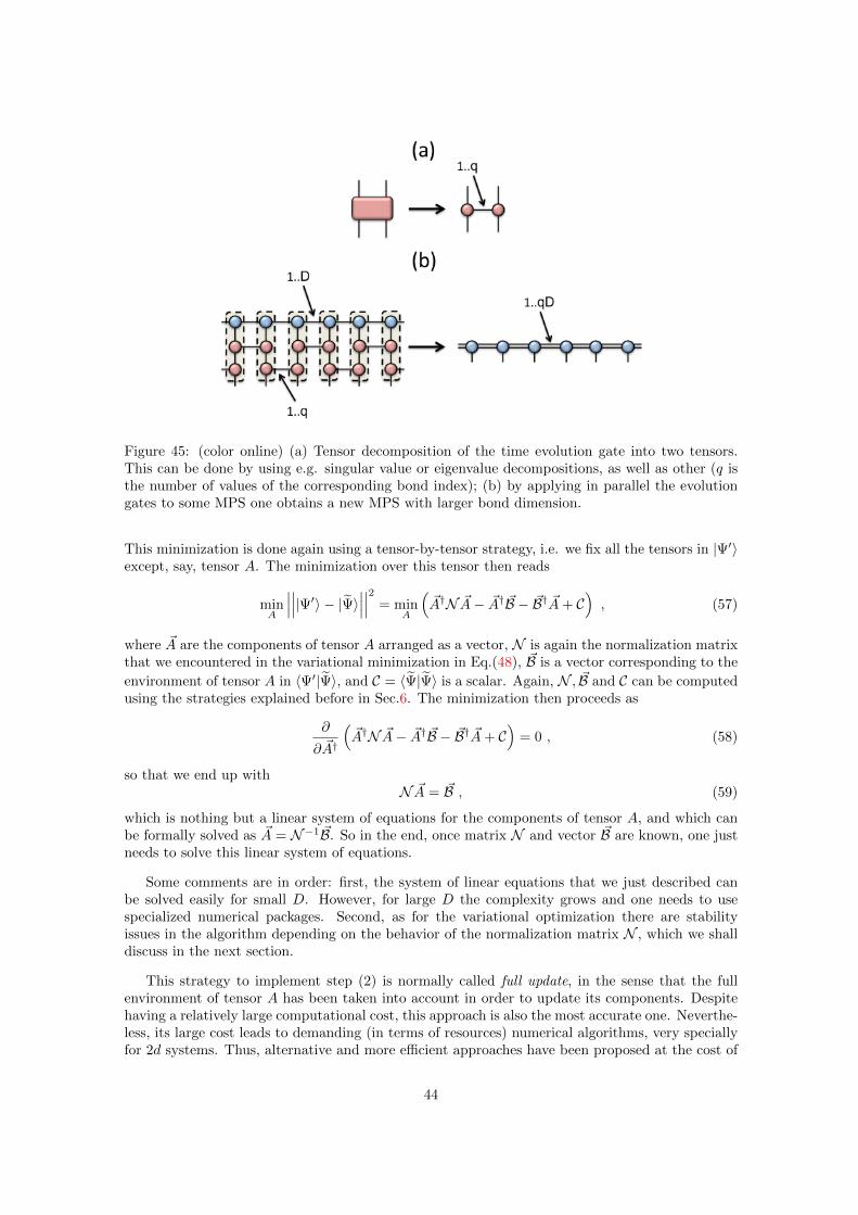
Figure 45: (color online) (a) Tensor decomposition of the time evolution gate into two tensors.This can be done by using e.g. singular value or eigenvalue decompositions, as well as other (q isthe number of values of the corresponding bond index); (b) by applying in parallel the evolutiongates to some MPS one obtains a new MPS with larger bond dimension.
This minimization is done again using a tensor-by-tensor strategy, i.e. we fix all the tensors in |Ψ′〉except, say, tensor A. The minimization over this tensor then reads
minA
∣∣∣∣∣∣|Ψ′〉 − |Ψ〉∣∣∣∣∣∣2 = minA
(~A†N ~A− ~A† ~B − ~B† ~A+ C
), (57)
where ~A are the components of tensor A arranged as a vector, N is again the normalization matrixthat we encountered in the variational minimization in Eq.(48), ~B is a vector corresponding to the
environment of tensor A in 〈Ψ′|Ψ〉, and C = 〈Ψ|Ψ〉 is a scalar. Again, N , ~B and C can be computedusing the strategies explained before in Sec.6. The minimization then proceeds as
∂
∂ ~A†
(~A†N ~A− ~A† ~B − ~B† ~A+ C
)= 0 , (58)
so that we end up withN ~A = ~B , (59)
which is nothing but a linear system of equations for the components of tensor A, and which canbe formally solved as ~A = N−1 ~B. So in the end, once matrix N and vector ~B are known, one justneeds to solve this linear system of equations.
Some comments are in order: first, the system of linear equations that we just described canbe solved easily for small D. However, for large D the complexity grows and one needs to usespecialized numerical packages. Second, as for the variational optimization there are stabilityissues in the algorithm depending on the behavior of the normalization matrix N , which we shalldiscuss in the next section.
This strategy to implement step (2) is normally called full update, in the sense that the fullenvironment of tensor A has been taken into account in order to update its components. Despitehaving a relatively large computational cost, this approach is also the most accurate one. Neverthe-less, its large cost leads to demanding (in terms of resources) numerical algorithms, very speciallyfor 2d systems. Thus, alternative and more efficient approaches have been proposed at the cost of
44

sacrificing part of the accuracy: these are the so-called simple update methods. In a broad sense,these methods avoid the full calculation of the environment of tensor A during its update, whichusually is the bottleneck of the calculation. Instead, they use some “simple” environment for whichalmost no calculation is needed. Such a “simple” environment implements a huge oversimplifica-tion of the effect of quantum correlations in the system, and in fact most of the time follows fromsome type of mean-field approximation (or Bethe lattice approximation [82]). This strategy turnsout to be really good and almost exact for 1d systems as long as the infinitesimal time step δτis sufficiently small, and leads to the so-called Time-Evolving Block Decimation (TEBD) method[13]. However, for 2d systems its “accuracy vs efficiency” tradeoff is still a matter of debate: resultsfor gapped phases are normally acceptable and can give a good idea of the physics of the systemat hand with a fast algorithm that allows to reach large values of D. But however, the accuracyof the results drops down substantially when approaching a quantum critical point, i.e. when thecorrelation length is large and the full effect of all the surrounding environment of a tensor isimportant. We shall not explain here more details about the simple update method, and refer thereader to Ref.[74] for more details.
7.3 Stability and the normalization matrix N .
A delicate issue in the numerics of the above two approaches is the conditioning of matrixN . Noticethat, by definition, this matrix is hermitian and positive since it can always be written asN = X†Xfor some matrix X (this is just a consequence of the ket-bra structure of the corresponding TN).Therefore, all its eigenvalues are positive. Taking this into account, one can identify two possibleproblems:
1. The matrix, even if computed exactly (as in MPS), has eigenvalues very close to zero.
2. The matrix can only be approximated (as in PEPS), and therefore it may have some negativeeigenvalues.
In either of the two cases, the corresponding solution to the generalized eigenvalue problemor linear system of equations may produce wrong results. If not somehow corrected, the errorusually amplifies over the iterations in the algorithm, hence killing the convergence and producinginstabilities. Therefore, it is really important to have, at every step, matrices N as accurate andas well conditioned as possible.
Depending on the situation there are several ways of getting around the above two problems.Some options are:
1. If the TN has no loops (e.g. MPS with open boundary conditions), then it is always possibleto choose an appropriate gauge for the tensors in which N = I. This is actually achievedby the canonical form in Fig.(18) for MPS with open boundary conditions. The algorithm isthus more stable and the problems to be solved are far more simple, yet the price to be paidis that one needs to compute this canonical form at every step.
2. If the TN has loops (e.g. PEPS), then one can think of adding/subtracting to N someinfinitesimal constant term proportional to the identity with the aim to kill eigenvalues closeto zero or slightly negative, i.e. N + εI with ε � 1. One can also think of making “ashermitian as possible” the matrix at every step by e.g. using (N + N †)/2 instead of N aslong as the introduced difference is small enough. Another option is to choose a gauge for thetensors in such a way that N is as close as possible to the identity (yet not exactly equal toit), and which can normally be achieved by using a quasi-canonical form for the TN, see e.g.
45

Ref.[75]. Finally, it is also possible to think of approximation schemes for N which preservethe hermitian and positive structure at every step, yet at the price of getting lower accuracy,see e.g. Ref.[83].
These are just some examples of “stabilizing tricks”. Of course, in a realistic situation one triesto combine all of them in order to make the algorithm as stable as possible.
8 Final remarks
Hopefully we offered here a plausible introduction to some key aspects of TN methods for quantummany-body systems for the non-experienced reader. A number of topics were addressed, includingsome important ideas to deal numerically with 1d systems using MPS and 2d systems using PEPS.Yet, what we explained here is only the top of the iceberg.
There are many things which were not covered in this introduction. For instance, we didnot enter into the detailed implementation of most algorithms (such as TEBD [13], iPEPS [32],and many more). We also did not talk about the very interesting properties of the MERA andits related numerical methods [21, 22]. Other important topics were not addressed, such as theimplementation of symmetries in TNs [36], how to deal with fermionic systems in 2d [38], andcontraction/update schemes based on Montecarlo sampling [23, 24, 25]. We did not talk eitherabout the continuum limit of a TN, which defines e.g. the family of continuous MPS [27], andwhich is of relevance as variational ansatz to simulate quantum field theories in the continuum.Also, we did not discuss 2d implementations of DMRG [39], as well as TN methods for thermalstates and dissipative systems [84]. From a more theoretical point of view, we did not explainthe deep relation between TNs and the entanglement spectrum [73], neither the relation to theholographic principle and the AdS/CFT correspondence [2] and other potential applications toquantum gravity [51]. Other important topics that we did not touch here are parent and uncleHamiltonians for 2d PEPS [85], as well as mathematical proofs for the connection between thermalstates of gapped local Hamiltonians and TNs [57].
The above are just some examples of topics that we believe to be important, but which were notdiscussed here because its explanation lies beyond our current purpose. In fact, new developmentsin the field appear almost on a daily basis, and sometimes in totally unforeseen and surprisingdirections. It is thus our hope that this paper helps the newcomers to digest better the big amountof literature and information already available on the exciting topic of Tensor Networks.
Acknowledgements The author acknowledges financial support from the Johannes-GutenbergUniversitat, as well as the participants of the DMRG101 Winter School 2012 in Taipei for inter-esting discussions which motivated this paper. Insightful comments by T. Nishino, G. Vidal, M.Rizzi, F. Verstraete, J. I. Cirac, M. C. Banuls and T. Xiang are also acknowledged.
References
[1] J. M. Maldecena, Adv. Theor. Math. Phys. 2, 231 (1998); S. S. Gubser, I. R. Klebanov, A. M.Polyakov, Phys. Lett. B 428, 105 (1998); E. Witten, Adv. Theor. Math. Phys. 2, 253 (1998).
[2] S. Ryu, T. Takayanagi, Phys. Rev. Lett. 96, 181602 (2006); B. Swingle, Phys. Rev. D 86,065007 (2012); G. Evenbly, G. Vidal, J. Stat. Phys. 145, 891-918 (2011); J. Molina-Vilaplana,JHEP05 024 (2013).
46

[3] J. Nagamatsu, N. Nakagawa, T. Muranaka, Y. Zenitani, J. Akimitsu, Nature 410 (6824) pp63-64 (2001).
[4] X.-G. Wen, Quantum Field Theory of Many-Body Systems, Oxford University Press (2004).
[5] G. Misguich, C. Lhuillier, Frustrated spin systems, H. T. Diep editor, World-Scientific (2005).
[6] T. Senthil, A. Vishwanath, L. Balents, S. Sachdev, M. P. A. Fisher, Science 303, 1490 (2004);T. Senthil, L. Balents, S. Sachdev, A. Vishwanath, M. P. A. Fisher, Phys. Rev. B 70, 144407(2004).
[7] A. Altand, B. Simons, Condensed Matter Field Theory. Cambridge University Press pp.58(2006).
[8] J. I. Cirac, F. Verstraete, J. Phys. A: Math. Theor. 42, 504004 (2009); F. Verstratete, J. I.Cirac, V. Murg, Adv. Phys. 57,143 (2008); R. Augusiak, F. M. Cucchietti, M. Lewenstein, inModern Theories of Many-Particle Systems in Condensed Matter Physics, Lect. Not. Phys. 843,245-294 (2012).
[9] S. R. White, Phys. Rev. Lett. 69, 28632866 (1992).
[10] S. R. White, Phys. Rev. B 48, 10345 (1992).
[11] D. Porras, F. Verstraete, J. I. Cirac, Phys. Rev. Lett. 93, 227205 (2004).
[12] A. J. Daley, C. Kollath, U. Schollwock, G. Vidal, J. Stat. Mech.: Theor. Exp. (2004) P04005.
[13] G. Vidal, Phys. Rev. Lett. 91, 147902 (2003); G. Vidal, Phys. Rev. Lett. 939, 040502 (2004).
[14] G. Vidal, Phys. Rev. Lett. 98, 070201 (2007); R. Orus, G. Vidal, Phys. Rev. B 78, 155117(2008).
[15] M. C. Banuls, M. B. Hastings, F. verstraete, J. I. Cirac, Phys. Rev. Lett. 102, 240603 (2009).
[16] F. Verstraete, J. I. Cirac, cond-mat/0407066.
[17] Z.-Cheng Gu, M. Levin, X.-Gang Wen, Phys. Rev. B 78, 205116 (2008).
[18] M. Levin, C. P. Nave, Phys. Rev. Lett. 99, 120601 (2007).
[19] T. Nishino, Y. Hieida, K. Okunishi, N. Maeshima, Y. Akutsu, A. Gendiar, Prog. Theor. Phys.105, No.3, 409-417 (2001).
[20] S. Anders, H. J. Briegel, W. Dur, New J. Phys. 9, 361 (2007).
[21] G. Vidal, Phys. Rev. Lett. 99, 220405 (2007); For an introduction, see e.g.: G. Vidal, chapterof the book Understanding Quantum Phase Transitions, edited by Lincoln D. Carr (Taylor &Francis, Boca Raton, 2010), arXiv:0912.1651v2.
[22] G. Evenbly, G. Vidal, arXiv:1210.1895.
[23] N. Schuch, M. M. Wolf, F. Verstraete, and J. I. Cirac, Phys. Rev. Lett. 100, 040501 (2008).
[24] F. Mezzacapo, N. Schuch, M. Boninsegni, J. I. Cirac New J. Phys. 11, 083026 (2009).
[25] A. W. Sandvik, G. Vidal, Phys. Rev. Lett. 99, 220602 (2007).
[26] Y. Shi, L. Duan, G. Vidal, Phys. Rev. A 74, 022320 (2006); L. Tagliacozzo, G. Evenbly,G. Vidal, Phys. Rev. B 80, 235127 (2009); P. Silvi, V.Giovannetti, S.Montangero, M.Rizzi, J.I. Cirac, R. Fazio, Phys. Rev. A 81, 062335 (2010); V. Murg, O. Legeza, R. M. Noack, F.Verstraete, Phys. Rev. B 82, 205105 (2010).
47
[27] Verstraete, F. and Cirac, J. I., Phys. Rev. Lett. 104, 190405 (2010); J. Haegeman, J. I. Cirac,T. J. Osborne, H. Verschelde, F. Verstraete, Phys. Rev. Lett. 105, 251601 (2010); J. Haegeman,T. J. Osborne, H. Verschelde, F. Verstraete, Phys. Rev. Lett. 110, 100402 (2013); C. Brockt,J. Haegeman, D. Jennings, T. J. Osborne, F. Verstraete, arXiv:1210.5401; J. Haegeman, J. I.Cirac, T. J. Osborne, F. Verstraete, arXiv:1211.3935; D. Jennings, J. Haegeman, T. J. Osborne,F. Verstraete, arXiv:1212.3833.
[28] J. Haegeman, J. I. Cirac, T. J. Osborne, I. Pizorn, H. Verschelde, F. Verstraete, Phys. Rev.Lett. 107, 070601 (2011).
[29] Z. Y. Xie, H. C. Jiang, Q. N. Chen, Z. Y. Weng, T. Xiang, Phys. Rev. Lett. 103, 160601(2009); H. H. Zhao, Z. Y. Xie, Q. N. Chen, Z. C. Wei, J. W. Cai, T. Xiang, Phys. Rev. B 81,174411 (2010).
[30] Z. Y. Xie, J. Chen, M. P. Qin, J. W. Zhu, L. P. Yang, T. Xiang, Phys. Rev. B 86, 045139(2012).
[31] I. P. McCulloch, arXiv:0804.2509; G. M. Crosswhite, A. C. Doherty, G. Vidal, Phys. Rev. B78, 035116 (2008).
[32] J. Jordan, R. Orus, G. Vidal, F. Verstraete, J. I. Cirac, Phys. Rev. Lett. 101, 250602 (2008);
[33] R. Orus, G. Vidal, Phys. Rev. B 80, 094403 (2009).
[34] N. Maeshima, Y. Hieida, Y. Akutsu, T. Nishino, K. Okunishi, Phys. Rev. E 64 016705 (2001);Y. Nishio, N. Maeshima, A. Gendiar, T. Nishino, cond-mat/0401115.
[35] P. Pippan, S. R. White, H. G. Evertz, Phys. Rev. B 81, 081103(R) (2010); B. Pirvu, F.Verstraete, G. Vidal, Phys. Rev. B 83, 125104 (2011).
[36] I. McCulloch, M. Gulacsi, Europhys. Lett. 57, 852 (2002); S. Singh, H.-Q. Zhou, G. Vidal,New J. Phys. 12 033029 (2010); S. Singh, R. N. C. Pfeifer, G. Vidal, Phys. Rev. A 82 050301,(2010); S. Singh, R. N. C. Pfeifer, G. Vidal, Phys. Rev. B 83 115125, (2011); B. Bauer, P.Corboz, R. Orus, M. Troyer, Phys. Rev. B 83, 125106 (2011); D. Perez-Garcıa, M.M. Wolf, M.Sanz, F. Verstraete, J. I. Cirac, Phys. Rev. Lett. 100, 167202 (2008); M. Sanz, M. M. Wolf, D.Perez-Garcıa, J. I. Cirac, Phys. Rev. A 79, 042308 (2009); N. Schuch, I. Cirac, D. Perez-Garcıa,Ann. Phys. 325, 2153 (2010); N. Schuch, I. Cirac, D. Perez-Garcıa, Phys. Rev. B 84, 165139(2011); A. Weichselbaum, Ann. of Phys. 327, 2972-3047 (2012).
[37] V. Murg, F. Verstraete, J. I. Cirac, Phys. Rev. A 75, 033605 (2007); J. Jordan, R. Orus, G.Vidal, Phys. Rev. B 79, 174515 (2009).
[38] P. Corboz, G. Evenbly, F. Verstraete, G. Vidal, Phys. Rev. A 81, 010303(R) (2010); C. V.Kraus, N. Schuch, F. Verstraete, G. Vidal, Phys. Rev. A 81, 052338 (2010); C. Pineda, T.Barthel, J. Eisert, Phys. Rev. A 81, 050303(R) (2010); P. Corboz, G. Vidal, Phys. Rev. B 80,165129 (2009); T. Barthel, C. Pineda, J. Eisert, Phys. Rev. A 80, 042333 (2009); Q.-Q. Shi,S.-Hao Li, J.-Hui Zhao, H.- Qiang Zhou, arXiv:0907.5520; P. Corboz, S. R. White, G. Vidal, M.Troyer, Phys. Rev. B 84, 041108 (2011); P. Corboz, R. Orus, B. Bauer, G. Vidal, Phys. Rev. B81, 165104 (2010); P. Corboz, S. Capponi, A. M. Lauchli, B. Bauer, R. Orus, EPL 98, 27005(2012).
[39] V. Murg, F. Verstraete, J. I. Cirac, Phys. Rev. B 79, 195119 (2009); G. Evenbly, G. Vidal,Phys. Rev. Lett. 104, 187203 (2010); S. Yan, D. A. Huse, S. R. White, Science 332 (6034),11731176 (2011); L. Wang, Z.-Cheng Gu, X.-Gang Wen, F. Verstraete, arXiv:1112.3331; F.Mezzacapo, Phys. Rev. B 86, 045115 (2012); F. Mezzacapo, M. Boninsegni, Phys. Rev. B 85,060402 (2012); S. Depenbrock, I. P. McCulloch, U. Schollwock, Phys. Rev. Lett. 109, 067201(2012).
48

[40] R.Orus, A.Doherty, G.Vidal, Phys. Rev. Lett. 102, 077203 (2009); S. Dusuel, M. Kamfor, R.Orus, K. P. Schmidt, J. Vidal, Phys. Rev. Lett. 106, 107203 (2011); M. D. Schulz, S. Dusuel,R. Orus, J. Vidal, K. P. Schmidt, New J. Phys. 14, 025005 (2012); X.-Chen, B.-Zeng, Z.-ChengGu, I. L. Chuang, X.-Gang Wen, Phys. Rev. B 82, 165119 (2010).
[41] O. Legeza, J. Solyom, Phys. Rev. B 68, 195116 (2003); J. Rissler, R. M. Noack, S. R. White,Chem. Phys. 323, 519-531(2006); O. Legeza, R. M. Noack, J. Solyom, L. Tincani, in Computa-tional Many-Particle Physics, Lect. Not. Phys. 739, 655-664 (2008); G. Barcza, O. Legeza, K.H. Marti, M. Reiher, Phys. Rev. A 83, 012508 (2011); K. H. Marti, B. Bauer, M. Reiher, M.Troyer, F. Verstraete, New J. Phys. 12 (2010) 103008; N. Nakatani, G. K.-Lic Chan, J. Chem.Phys. 138, 134113 (2013).
[42] T. M. R. Byrnes, P. Sriganesh, R. J. Bursill, C. J. Hamer, Phys. Rev. D 66 013002 (2002); T.Sugihara, J. High En. Phys. 07 022 (2005); L. Tagliacozzo, G. Vidal, Phys. Rev. B 83 115127(2011); M. C. Banuls, K. Cichy, K. Jansen, J. I. Cirac, arXiv:1305.3765.
[43] W. Hackbusch, Tensor spaces and numerical tensor calculus, Springer (2012).
[44] J. Cullum, R. Willoughby, Lanczos Algorithms for Large Symmetric Eigenvalue Computa-tions, Vol. 1: Theory (Classics in applied mathematics), Society for Industrial and AppliedMathematics (2002).
[45] J. Oitmaa, C. Hamer, W. Zheng, Series Expansion Methods for Strongly Interacting LatticeModels, Cambridge University Press (2006).
[46] V. Vedral, New J. Phys. 6, 22, pp1-25 (2004).
[47] M. P. Nightingale, J. C. Umrigar, Quantum Monte Carlo Methods in Physics and Chemistry.Springer (1999).
[48] F. Wegner, Annalen der Physik (Leipzig) 3, 77-91 (1994); J. Stein, J. of Stat. Phys. 88, 487-511 (1997); C. Knetter, G. S. Uhrig, Europ. Phys. J. B 13, 209-225 (2000); C. Knetter, K. P.Schmidt, G. S. Uhrig, J. of Phys. A 36, 7889-7907 (2003).
[49] J. C. Cramer, Essentials of Computational Chemistry, Chichester: John Wiley & Sons, Ltd..pp.191232 (2002).
[50] R. G. Parr, W. Yang, Density-Functional Theory of Atoms and Molecules, New York: OxfordUniversity Press (1989).
[51] M. Van Raamsdonk, arXiv:0907.2939; M. van Raamsdonk, Gen. Rel. Grav. 42:2323-2329 (2010) and Int. J. Mod. Phys. D 19:2429-2435 (2010); J. Maldacena, L. Susskind,arXiv:1306.0533.
[52] See e.g. https://en.wikipedia.org/wiki/Observable universe
[53] T. Xiang, J. Lou, Z. Su, Phys. Rev. B 64, 104414 (2001); O. Legaza, J. Solyom, cond-mat/0305336; O. Legaza, J. Solyom, Phys. Rev. B 70, 205118 (2004); G. Vidal, J. I. Latorre, E.Rico, A. Kitaev, Phys. Rev. Lett. 90 227902 (2003); P. Calabrese, J. Cardy, JSTAT 0406:P06002(2004); M. Srednicki, Phys. Rev. Lett. 71, 666 (1993); M. Plenio, J. Eisert, J. Dreißig, M. Cramer,Phys. Rev. Lett. 94, 060503 (2005).
[54] M. M. Wolf, Phys. Rev. Lett. 96, 010404 (2006).
[55] M. P. A. Fisher, O. I. Motrunich, D. N. Sheng, Proc. 24th Solvay conf. (2008).
[56] A. B. Kallin, M. B. Hastings, R. G. Melko, R. R. P. Singh, Phys. Rev. B 84, 165134 (2011).
[57] M. B. Hastings, Phys. Rev. B 73, 085115 (2006); M.M. Wolf, F. Verstraete, M.B. Hastings,J.I. Cirac, Phys. Rev. Lett. 100, 070502 (2008).
49

[58] D. Poulin, A. Qarry, R. D. Somma, F. Verstraete, Phys. Rev. Lett. 106, 170501 (2011).
[59] See e.g. https://en.wikipedia.org/wiki/Age of the universe
[60] M. Fannes, B. Nachtergaele, R. F. Werner, Commun. Math. Phys. 144, 443-490 (1992); A.Klumper, A. Schadschneider, J. Zittartz, J. Phys. A 24, L955 (1991); A. Klumper, A. Schad-schneider, J. Zittartz, Europhys. Lett. 24, 293 (1993).
[61] T. Nishino, K. Okunishi, J. Phys. Soc. Jap. 64, 4084-4087 (1995).
[62] U. Schollwock, Rev. Mod. Phys. 77, 259 (2005); U. Schollwock, Ann. Phys. 326, 96 (2011).
[63] D. M. Greenberger, M. A. Horne, A. Zeilinger, in Bell’s Theorem, Quantum Theory, andConceptions of the Universe, M. Kafatos (Ed.), Kluwer, Dordrecht, 69-72 (1989).
[64] R. Raussendorf, H. J. Briegel, Phys. Rev. Lett. 86, 5188 (2001).
[65] A. Affleck, T. Kennedy, E. H. Lieb, H. Tasaki, Commun. Math. Phys. 115, 477 (1988); A.Affleck, T. Kennedy, E. H. Lieb, H. Tasaki, Phys. Rev. Lett. 59, 799 (1988).
[66] C. K. Majumdar, D. K. Ghosh, J. Math. Phys. 10, 1388 (1969).
[67] T. Nishino, K. Okunishi, J. Phys. Soc. Jpn. 65 pp. 891-894 (1996); T. Nishino, K. Okunishi,J. Phys. Soc. Jp. 66, 3040 (1997).
[68] R. Orus, Phys. Rev. B 85, 205117 (2012).
[69] F. Verstraete, M. M. Wolf, D. Perez-Garcıa, J. I. Cirac, Phys. Rev. Lett. 96, 220601 (2006).
[70] S. Sachdev, Quantum Phase Transitions, Cambridge University Press, 2nd Edition (2011).
[71] N. Schuch, M. M. Wolf, F. Verstraete, J. I. Cirac, Phys. Rev. Lett. 98, 140506 (2007).
[72] C. H. Papadimitrou, Computational Complexity, Addison Wesley (1993).
[73] H. Li, F. D. M Haldane, Phys. Rev. Lett. 101, 010504 (2008); J. I. Cirac, D. Poilblanc, N.Schuch, F. Verstraete, Phys. Rev. B 83, 245134 (2011).
[74] H. C. Jiang, Z. Y. Weng, T. Xiang, Phys. Rev. Lett. 101, 090603 (2008).
[75] H. Kalis, D. Klagges, R. Orus, K.P. Schmidt, Phys. Rev. A 86, 022317 (2012); R. Orus, H.Kalis, M. Bornemann, K. P. Schmidt, arXiv:1211.4054 (to appear in PRA).
[76] A. Y. Kitaev, Ann. Phys. 303, 2 (2003).
[77] J. B. Kogut, Rev. Mod. Phys. 51, pp659-713 (1979).
[78] Anderson, P. W. Science 235, 1196-1198 (1987).
[79] T.-Chieh Wei, I. Affleck, R. Raussendorf, Phys. Rev. Lett. 106, 070501 (2011).
[80] R. J. Baxter, Physica A 106, pp18-27 (1981); R. J. Baxter, Exactly Solved Models in StatisticalMechanics, Academic Press, London, (1982); R. J. Baxter, J. Math. Phys. 9, 650 (1968); R.J.Baxter, J. Stat. Phys. 19 461 (1978).
[81] M. Suzuki, Prog. Theor. Phys. 56, 1454 (1976).
[82] W. Li, J. von Delft, T. Xiang, Phys. Rev. B 86, 195137 (2012).
[83] I. Pizorn, L. Wang, F. Verstraete, Phys. Rev. A 83, 052321 (2011).
50

[84] R. J. Bursill, T. Xiang, G. A. Gehring, J. Phys.: Cond. Mat. 8 L583-L590 (1996); X. Wang,T. Xiang, Phys. Rev. B 56, 5061 (1997); N. Shibata, J. Phys. Soc. Jpn. 66, 2221 (1997); M.Zwolak, G. Vidal, Phys. Rev. Lett. 93, 207205 (2004); F. Verstraete, J. J. Garcia-Ripoll, J. I.Cirac, Phys. Rev. Lett. 93, 207204 (2004); P. Czarnik, L. Cincio, J. Dziarmaga, Phys. Rev. B86, 245101 (2012).
[85] C. Fernandez-Gonzalez, N. Schuch, M. M. Wolf, J. I. Cirac, D. Perez-Garcıa, Phys. Rev. Lett.109, 260401 (2012).
51


![Convex Coupled Matrix and Tensor Completion …arXiv:1705.05197v2 [stat.ML] 14 Jun 2018 Convex Coupled Matrix and Tensor Completion Kishan Wimalawarne Bioinformatics Center, Institute](https://img.dokumen.tips/doc/110x75/5e60bc431036ec2ab9156b98/convex-coupled-matrix-and-tensor-completion-arxiv170505197v2-statml-14-jun.jpg)