A Practical Guide to GIS in AutoCAD Civil 3D...iv A Practical Guide to GIS in AutoCAD Civil 3D 2018 Introduction Congratulations on choosing this course to help you learn how to use

A Practical Guide to GIS in AutoCAD® Civil 3D® 2018

Rick Ellis and Russell Martin

A CADapult Press Publication

ii

Copyright Copyright © CADapult Press, Inc. 2017 All rights reserved. No part of this publication may be reproduced in any form, or by any means electronic, mechanical, recording, photocopying, or otherwise, without written permission from the publisher, except for brief quotations used in reviews, or for marketing purposes specific to the promotion of this work. ISBN: 978-1-934865-34-7 Although CADapult Press has made every attempt to ensure the accuracy of the contents of this book, the publisher and author make no representations or warranty with respect to accuracy or completeness of the contents in this book, including without limitation warranties of fitness for a particular purpose. The datasets included in this book are for training purposes only. Autodesk screen shots reprinted with the permission of Autodesk, Inc. Autodesk, AutoCAD, DWG, the DWG logo, Civil 3D and AutoCAD Map 3D are registered trademarks or trademarks of Autodesk, Inc., and/or its subsidiaries and/or affiliates in the USA and other countries. All other trademarks are the property of their respective owners. Published in the United States of America by: CADapult Press (503) 829-8929 [email protected] Printed and manufactured in the United States of America

iii

About the Authors Rick Ellis has worked with and taught AutoCAD Civil 3D, along with Map 3D and other Autodesk products since the mid-90s. He is the Author of several critically acclaimed books on AutoCAD Civil 3D, Map 3D and Land Desktop. Rick continues to use AutoCAD Civil 3D on projects in a production environment, in addition to teaching classes to organizations both large and small. This practical background and approach has made him an award winning speaker at Autodesk University, a member of the national speaker team for the AUGI CAD Camps and a sought after instructor by organizations around the world. Rick can be reached at: [email protected] Russell Martin is an independent consultant who has worked with CAD, GIS and cartographic design tools since 1985. He has taught AutoCAD and AutoCAD Map 3D in small classrooms and at large events such as Autodesk University. Russell has co-authored several books on AutoCAD Map 3D, and has served as technical editor of many other books on CAD, computer graphics, Land Desktop and Civil 3D. Russell also performs design, production mapping and GIS analysis services for a diverse client base, both public and private. He uses AutoCAD, Map 3D and Civil 3D tools daily, to produce maps and graphics which clearly communicate complex quantitative data. Russell can be reached at: [email protected] Exercise Data CADapult Press would like to thank the City of Springfield, Oregon for providing the data for this book. The dataset provided is for illustration purposes only. While it is based on real world information to add relevance to the exercises, it has been altered and modified to more effectively demonstrate certain features as well as to protect all parties involved. The data should not be used for any project work and may not represent actual places or things. It is prohibited to redistribute this data beyond your personal use as a component of training.

iv

A Practical Guide to GIS in AutoCAD Civil 3D 2018 Introduction Congratulations on choosing this course to help you learn how to use GIS in AutoCAD Civil 3D 2018. The term “practical” is used in the title because this course focuses on what you need to effectively use the GIS tools in AutoCAD Civil 3D 2018, and does not complicate your learning experience with unnecessary details of every feature in the product. Should you want to pursue aspects of features and functionality in greater detail than provided in this course, you are directed and guided to that information. Each lesson contains the concepts and principles of each feature to provide you with the background and foundation of knowledge that you need to complete the lesson. You then work through real world exercises to reinforce your understanding and provide you with practice on common tasks that other professionals are performing with AutoCAD Civil 3D 2018 in the workplace every day. You can take the lessons in this course in whatever order is appropriate for your personal needs. If you want to concentrate on specific features, the lesson for those features does not require that you complete prior lessons. With this course organization, you can customize your own individual approach to learning AutoCAD Civil 3D. When you complete this course, you will be armed with the background and knowledge to apply AutoCAD Civil 3D to your job tasks, and become more effective and productive in your job. Course Objectives The objectives of this course are performance based. In other words, once you have completed the course, you will be able to perform each objective listed. If you are already familiar with AutoCAD Civil 3D, you will be able to analyze your existing workflows, and make changes to improve your performance based on the tools and features that you learn and practice in this course. After completing this course, you will be able to:

• Work with coordinate systems • Clean drawings with common geometry errors • Insert rectified raster images • Work with a variety of attribute data • Apply object classification to your mapping system • Import GIS data from a variety of sources • Create surfaces and pipe networks directly from GIS data • Export geometry and attribute data to other GIS formats • Export Civil 3D objects to other GIS formats • Connect directly to GIS data • Connect to raster surface data • Attach and query source drawings • Save changes to attached source drawings • Extract data for reports and quantity takeoffs • Create, manage and analyze topologies • Utilize Dynamic Viewport Tools • Produce sophisticated map books

v

Prerequisites Before starting this course, you should have a basic working knowledge of AutoCAD. A deep understanding of AutoCAD is not required, but you should be able to:

• Pan and Zoom in the AutoCAD drawing screen. • Describe what layers are in AutoCAD, and change the current layer. • Create basic CAD geometry, such as lines, polylines and circles. • Use Object Snaps. • Describe what blocks are, and how to insert them. • Perform basic CAD editing functions such as Erase, Copy, and Move.

If you are not familiar with these functions, you can refer to the AutoCAD Help system throughout the course to gain the fundamental skills needed to complete the exercises. Conventions The course uses the following icons and formatting to draw your attention to guidelines that increase your effectiveness in AutoCAD Civil 3D, or provide deeper insight into a subject.

The magnifying glass indicates that this text provides deeper insights into the subject.

The compass indicates that this text provides guidance that is based on the experience of other users of AutoCAD Civil 3D. This guidance is often in the form of how to perform a task more efficiently.

The warning indicates that a specific exercise might not function properly on 64 bit operating systems.

The workspace icon indicates the Workspace that will be used in the upcoming exercise.

vi

Downloading and Installing the Datasets In order to perform the exercises in this book, you must download a zip file and install the datasets. Type the address below into your web browser to load the page where you can download the dataset. www.cadapult-software.com/data If you are using a previous version of Civil 3D you can download a previous version of the dataset to use with this book. Unzip the Files Unzip the file APG_GIS2018.zip directly to the C drive. The zip file will create the following folder structure: C:\A Practical Guide\GIS in Civil 3D 2018\Chapter Number\Files for Exercises

Exercises The exercises in this course have been carefully chosen and designed to represent common tasks that are performed by mapping and GIS professionals. The data included in the exercises are typical drawings and maps used by local governments and municipalities. You work with road networks, parcel maps, sewer collection systems, water distribution systems, aerial photos, raster surfaces, and much more. Exercises provide higher level process information throughout the exercise tasks. You are given information about not only what to do, but why you are doing it. In most cases, an image is included to help guide you. 64 Bit Database Drivers On 64 bit systems, exercises that require a connection to an ODBC database need to have the proper drivers from Microsoft installed. If your system does not have these installed, you can download them from Microsoft. Go to [ http://www.microsoft.com ] and search for Microsoft Access Database Engine. Be sure to download the 64 bit version of the Microsoft Access Database Engine. You do not need to have Microsoft Office installed to install these drivers or to complete the exercise in this book. However, if you have Microsoft Office installed it will need to be the 64 bit version of Office for the 64 bit drivers to install.

vii

Table of Contents

Chapter 1 AutoCAD Civil 3D User Interface for GIS ...............................................................................1

1.1 Exploring the Civil 3D Tools for GIS .......................................................................................................2

1.1.1 Navigating the Civil 3D Interface for GIS .......................................................................... 10

Chapter 2 Creating Map Geometry ....................................................................................................... 13

2.1 Lesson: Establishing Coordinate Systems in Drawings ...................................................................... 14

2.1.1 Assigning a Coordinate System ....................................................................................... 19

2.1.2 Coordinate Tracking ......................................................................................................... 20

2.1.3 Digitizing Points ................................................................................................................ 21

2.2 Lesson: Creating and Inquiring COGO Data ...................................................................................... 23

2.2.1 Drawing with Transparent Commands ............................................................................. 26

2.2.2 Line and Arc Information .................................................................................................. 28

2.2.3 Angle Information ............................................................................................................. 29

2.2.4 Continuous Distance ........................................................................................................ 29

2.2.5 Continuous Distance from a Base Point ........................................................................... 30

2.2.6 Add Distance .................................................................................................................... 31

2.2.7 List Slope .......................................................................................................................... 31

2.3 Lesson: Using Drawing Cleanup ......................................................................................................... 33

2.3.1 Break Crossing Objects .................................................................................................... 38

2.3.2 Extend Undershoots ......................................................................................................... 42

2.3.3 Delete Duplicates ............................................................................................................. 43

2.3.4 Zero Length Objects ......................................................................................................... 45

2.3.5 Dissolve Pseudo Nodes ................................................................................................... 46

2.3.6 Simplifying Objects ........................................................................................................... 47

Chapter 3 Working with Attribute Data ................................................................................................. 51

3.1 Lesson: Attribute Data Concepts ......................................................................................................... 52

3.2 Lesson: Defining Object Data Tables .................................................................................................. 57

3.2.1 Creating Object Data Tables ............................................................................................ 61

3.3 Lesson: Attaching Object Data to Objects ........................................................................................... 66

3.3.1 Attaching Object Data to Objects ..................................................................................... 70

3.3.2 Attaching Object Data While Digitizing ............................................................................. 72

3.4 Lesson: Editing Object Data and Object Data Tables ......................................................................... 75

3.4.1 Editing Object Data ........................................................................................................... 80

3.4.2 Editing Object Data Tables ............................................................................................... 82

viii

3.5 Lesson: Attaching External Databases ................................................................................................ 84

3.5.1 Attaching External Databases ........................................................................................... 88

3.6 Lesson: Working with Data View .......................................................................................................... 89

3.6.1 Navigating in the Data View Table .................................................................................... 92

3.6.2 Applying SQL Filters ......................................................................................................... 93

3.7 Lesson: Defining a Link Template and Generating Links ..................................................................... 98

3.7.1 Defining a Link Template ................................................................................................ 104

3.7.2 Attaching Database Data to Existing Objects ................................................................. 105

3.7.3 Attaching Database Data While Digitizing ...................................................................... 107

3.7.4 Generating Links to Existing Blocks ................................................................................ 109

3.7.5 Highlighting objects by selecting records ........................................................................ 110

3.7.6 Highlighting table records by selecting objects ............................................................... 112

3.7.7 Using Spatial Filters ........................................................................................................ 113

3.8 Lesson: Establishing the Dynamic Annotation Environment .............................................................. 115

3.8.1 Defining an Annotation Template .................................................................................... 119

3.9 Lesson: Inserting and Managing Dynamic Annotation ....................................................................... 122

3.9.1 Annotating Objects .......................................................................................................... 125

3.9.2 Annotating Multiple Values ............................................................................................. 126

3.9.3 Updating Annotation........................................................................................................ 129

3.9.4 Rotating Annotation to Align with Objects ....................................................................... 130

3.9.5 Adding Text to Annotation Expressions .......................................................................... 132

3.9.6 Adding the Inch Symbol (") ............................................................................................. 133

3.9.7 Adding Length to the Annotation Template .................................................................... 134

3.9.8 Controlling Precision ....................................................................................................... 136

Chapter 4 Object Classification ........................................................................................................... 139

4.1 Lesson: Creating Object Classification Definition Files and Object Classes ..................................... 140

4.1.1 Log in as SuperUser ....................................................................................................... 145

4.1.2 Create a New Definition File ........................................................................................... 146

4.1.3 Define an Object Class ................................................................................................... 147

4.2 Lesson: Classifying Existing Objects and Validating Standards ........................................................ 152

4.2.1 Classifying Existing Objects ............................................................................................ 156

4.2.2 Validating Classified Objects .......................................................................................... 157

4.3 Lesson: Creating New Classified Objects .......................................................................................... 158

4.3.1 Creating New Classified Objects .................................................................................... 160

ix

Chapter 5 Importing and Exporting .................................................................................................... 163

5.1 Lesson: Importing GIS Data ............................................................................................................... 164

5.1.1 Importing an ArcInfo Coverage ...................................................................................... 167

5.1.2 Importing Polygons from an ArcView Shapefile ............................................................. 172

5.1.3 Creating Centroids .......................................................................................................... 177

5.2 Lesson: Exporting GIS Data .............................................................................................................. 179

5.2.1 Exporting Polygons to a SHP file ................................................................................... 183

5.2.2 Export to and SDF File ................................................................................................... 185

5.3 Importing GIS Data as Civil 3D Objects ............................................................................................. 189

5.3.1 Creating a Surface from a Shapefile .............................................................................. 191

5.3.2 Creating a Pipe Network from a SHP ............................................................................. 195

5.4 Exporting Civil 3D Objects as GIS Data ............................................................................................. 203

5.4.1 Exporting Civil 3D Objects to an SDF File ...................................................................... 204

Chapter 6 Connecting to Feature Sources ......................................................................................... 207

6.1 Lesson: Feature Source Concepts .................................................................................................... 208

6.2 Lesson: Connecting to SDF and SHP ................................................................................................ 212

6.2.1 Connect to and Add SDF Data ....................................................................................... 216

6.2.2 Connect to and Add SHP Data ....................................................................................... 219

6.3 Lesson: Working with Feature Layers ................................................................................................ 222

6.3.1 Working with Feature Layers .......................................................................................... 226

6.4 Lesson: Connecting to ODBC Point Feature Sources ....................................................................... 229

6.4.1 Create a System DSN .................................................................................................... 232

6.4.2 Connect to a DSN, and Add Points to a Map ................................................................. 234

Chapter 7 Using Raster Images in Maps ............................................................................................ 237

7.1 Lesson: Inserting Raster Images ....................................................................................................... 238

7.1.1 Inserting a Correlated Image .......................................................................................... 243

7.2 Lesson: Managing Raster Images .................................................................................................... 245

7.2.1 Adjust Image Display Properties .................................................................................... 248

7.2.2 Clipping Images .............................................................................................................. 248

7.2.3 Adding an Online Map .................................................................................................... 250

7.3 Lesson: Connecting to Raster and Raster Surfaces .......................................................................... 253

7.3.1 Connecting to an Aerial Photo ........................................................................................ 258

7.3.2 Connecting to a Raster Surface ..................................................................................... 260

x

Chapter 8 Stylizing Features ................................................................................................................ 263

8.1 Lesson: Stylizing Lines, Points, and Polygons ................................................................................... 264

8.1.1 Stylizing Polygon Features ............................................................................................. 269

8.1.2 Stylizing Line Features .................................................................................................... 273

8.1.3 Stylizing and Labeling Point Features............................................................................. 274

8.2 Lesson: Stylizing Raster Surfaces ...................................................................................................... 277

8.2.1 Stylizing Raster Features ................................................................................................ 282

8.2.2 Creating Contours from a Raster Surface ...................................................................... 284

8.3 Lesson: Creating Scale Dependent Styles ......................................................................................... 285

8.3.1 Working with Scale Dependent Styles ............................................................................ 289

8.4 Lesson: Applying Themes to Feature Layers ..................................................................................... 292

8.4.1 Thematic Mapping of Linear Objects with Object Data ................................................... 296

8.4.2 Thematic Mapping of Polygon Features ......................................................................... 299

Chapter 9 Working with Features ........................................................................................................ 301

9.1 Lesson: Creating Feature Filters and Feature Queries ...................................................................... 302

9.1.1 Preforming a Filter to Select ........................................................................................... 306

9.1.2 Preforming a Feature Query ........................................................................................... 307

9.2 Lesson: Editing Feature Geometry and Attributes ............................................................................. 309

9.2.1 Editing Features .............................................................................................................. 314

9.3 Lesson: Creating Joins ....................................................................................................................... 318

9.3.1 Create a System DSN ..................................................................................................... 323

9.3.2 Join Tables, and Create a Thematic Map ....................................................................... 325

9.4 Lesson: Using Constraints .................................................................................................................. 330

9.4.1 Working with Constraints ................................................................................................ 334

9.5 Lesson: Bulk Copy Between Feature Sources ................................................................................... 338

9.5.1 Exporting an SHP to an SDF .......................................................................................... 342

9.5.2 Bulk Copy from an SDF to an SHP ................................................................................. 343

Chapter 10 Using Attached Source Drawings and Queries ................................................................ 347

10.1 Lesson: Managing Source Drawings .................................................................................................. 348

10.1.1 Managing Source Drawings ............................................................................................ 354

10.2 Lesson: Executing Location and Property Queries ............................................................................ 359

10.2.1 Executing Location Queries ............................................................................................ 366

10.2.2 Executing Property Queries ............................................................................................ 372

10.2.3 Executing Compound Queries ........................................................................................ 374

xi

10.3 Lesson: Executing Data Queries ....................................................................................................... 378

10.3.1 Query by Pipe Size from Object Data ............................................................................ 381

10.4 Lesson: Altering Properties During Queries ...................................................................................... 386

10.4.1 Execute a Query with a Property Alteration ................................................................... 389

10.5 Lesson: Using Save-Back .................................................................................................................. 392

10.5.1 Execute Save-Back to Save Changes to an Attached Source Drawing ........................ 398

10.6 Lesson: Working with Multiple Coordinate Systems .......................................................................... 401

10.6.1 Working with Source Drawings in Multiple Coordinate Systems.................................... 404

Chapter 11 Working with Topologies ................................................................................................... 407

11.1 Lesson: Creating Network Topologies ............................................................................................... 408

11.1.1 Creating a Network Topology ......................................................................................... 413

11.2 Lesson: Creating Polygon Topologies ............................................................................................... 417

11.2.1 Creating a Polygon Topology ......................................................................................... 421

11.3 Lesson: Performing Topology Analysis.............................................................................................. 427

11.3.1 Network Analysis ............................................................................................................ 431

11.3.2 Performing a Buffer Analysis .......................................................................................... 433

11.3.3 Performing an Overlay Analysis ..................................................................................... 436

Chapter 12 Map Output .......................................................................................................................... 441

12.1 Lesson: Adding Dynamic Legends, Scale Bars and North Arrows .................................................... 442

12.1.1 Adding a Dynamic Legend to a Layout .......................................................................... 446

12.1.2 Adding a Dynamic Scale Bar to a Layout ....................................................................... 449

12.1.3 Adding a Dynamic North Arrow to a Layout ................................................................... 452

12.1.4 Adding a Coordinate System Grid to a Layout ............................................................... 454

12.2 Lesson: Creating Map Books ............................................................................................................. 456

12.2.1 Creating a Map Book ...................................................................................................... 460

12.2.2 Navigating Through the Map Book ................................................................................. 464

12.2.3 Publishing the Map Book ................................................................................................ 465

Chapter: Importing and Exporting

164 Lesson: Importing GIS Data

5.1 Lesson: Importing GIS Data

Introduction Importing GIS file formats into Civil 3D opens the door to a tremendous amount of data. Much of this data is free, and can be integrated into your mapping system. In this lesson, you begin by learning the formats and types of data that can be imported into Civil 3D, and guidelines around integrating other mapping data into your mapping system. You then import an ArcView SHP file into Civil 3D.

Key Concepts Concepts and key terms covered in this lesson are:

• Import o Geometry o Attributes o Coordinate Systems

• Import dialog box Objectives After completing this lesson, you will be able to:

• Describe what Map Import is. • List the components that can be imported, and how Civil 3D interprets incoming data. • Identify and explain the tools used to import GIS data. • Import street segments with Object Data. • Import zoning polygons with an external data source.


Lesson: Importing GIS Data 165

About Importing GIS Data into Civil 3D GIS Data generally contains three types of data: geometry, attributes, and the coordinate system it was created in. Using the map import tools, you can define how Civil 3D interprets and imports all three types of data.

The Map Import commands are used to convert other GIS formats into AutoCAD objects with attributes. These new AutoCAD objects are saved in the drawing file, with no link to the original GIS source.

Geometry All GIS formats are different. Civil 3D imports the data in such a way as to represent the native format as closely as possible. An example of this functionality is when importing line data from an ArcView shape file, any segments in the incoming file that have vertexes are imported as polylines, while those that are simple lines with a start and endpoint are imported as lines.

Points can be imported as either AutoCAD points, or blocks that are defined in the drawing.

Attributes Attributes that are associated with incoming data can be mapped to Object Data, or can be imported to an attached data source, such as a Microsoft Access database table, and linked to the objects at the same time.

Coordinate Systems If the incoming file has coordinate system information associated with it, either within the file itself, or a companion file, Civil 3D will read this information and convert the coordinates to the target drawing file. If there is no coordinate system information in the incoming file, you can assign a coordinate system to it during the import procedure.

Spatial Filters Some GIS applications can manage larger data sets than can be reasonably managed within Civil 3D. Spatial filters enable you to limit the amount of data that you import based on a location in the current map.

Guidelines for Preparing for Map Import You can start a new drawing and simply import data. In most cases, you want to prepare a target drawing with layers, Object Data tables, or attached data sources that will receive the incoming data. This is especially true if your office has mapping standards that must be adhered to, or if you are importing into an existing drawing that already has all the layers, Object Data tables, or attached data sources present.

Another important point when preparing for an import is to have some familiarity with the incoming data. This may come from metadata or documentation of some kind. The best way to qualify the incoming data is to use the native application to review. However, this is not always possible, in which case the import process might be a trial and error process until you can make the correct settings for the final import.

Civil 3D can also connect to data as a feature source and work with these files in their native format. This functionality is covered in another lesson.



The Import Interface Once the target file is prepared, and the incoming data is qualified, the entire import procedure is performed in a single interface with various dialog boxes for the settings.

If you perform the same type of import regularly, you can save a profile of the settings and load the profile each time you perform an import. You can also create a drawing template that has all of the definitions such as Object Data tables, layers, blocks and so on.



Exercises: Import Data from Other GIS Formats In these exercises you will import street centerlines that were sent to you as an E00 file. An ArcInfo coverage may either be stored as a directory of related files, or exported into a single E00 export file from ArcInfo or ArcGIS, as in this exercise.

Then you will, import parcel polygons from an ArcView Shapefile and convert their coordinate system.

Finally, you will create centroids and move the attached data from each polyline to the corresponding centroid. This is the first step in the process of cleaning the geometry, an important process whenever base map data is imported.

The use of the import command is very similar for all the different types of supported GIS data file formats. However, there are some differences depending on the type of geometry that is contained in those files (points, lines, or polygons).

You do the following:

• Import streets from an E00 file. • Import parcels from an ArcView shape file and convert its coordinate system. • Create centroids for the parcel polygons.

5.1.1 Importing an ArcInfo Coverage

For these exercises you should be in the Planning and Analysis workspace

In this exercise you will import street centerlines that were sent to you as an E00 file. An ArcInfo coverage may either be stored as a directory of related files, or exported into a single E00 export file from ArcInfo or ArcGIS, as in this exercise.

1. Press Ctrl + N and select the template map2d.dwt from the folder Map Book Templates, to start a new, blank drawing.

2. Select Ribbon: Insert ⇒ Import ⇒ Map Import.



The Import Location dialog box opens.

3. Set the file type to ESRI ArcInfo Export (E00).

4. Browse to the Chapter 05 folder, select streets.e00, and click <<OK>>.

In the Import dialog box you can configure the Layer, Coordinate Conversion, and Data options that you wish to use to import the information into AutoCAD.

5. Ensure that the STREETS_arc Input Layer is selected.

6. Click on the Drawing Layer field in the STREETS_arc row, to activate the More button <<…>>.

7. Click the More button <<…>> to launch the Layer Mapping dialog box.



Here you can choose to import the drawing objects onto an existing layer, create a new layer, or select a column of data from the file that you are importing to determine the layer names. This last option will allow you to do some basic thematic mapping during the import of the objects. For example, if you were importing parcel data and that data set had a column for zoning. You could have the import command create a new layer for each zoning type and place each parcel on the appropriate layer for its zoning designation. (See Additional Exercises at the end of this chapter for more information).

In this exercise, you will place all of the streets on one new layer.

8. Choose the Create on new layer option to activate the text box.

9. Enter "Streets" for the layer name.

10. Click <<OK>> to return to the Import dialog box.

11. Click on the Data field in the STREETS_arc row to activate the More button <<…>>.

12. Click the More button <<…>> to launch the Attribute Data dialog box.

Here you specify what attribute data to import and where to store it. You can enter the desired name for the Object Data Table and select the desired fields to import. This is the step that allows you to bring the intelligence of the GIS file along with the geometry into AutoCAD. By creating the object data table and populating it with the information provided in



the coverage you will be able to click on a street and find the street name, type, speed limit, and any other information that was added by the GIS department. This will also allow you to edit the geometry and data from the GIS file in AutoCAD and then export it back to any of the supported GIS formats without losing any of the attached data. If you leave the Data option set to None or Do not import attribute data, then you will only import the geometry of the file and you will lose all of the attached information.

13. Choose the Create object data option to activate the Object Data section.

14. Change the Object Data table name to Streets.

15. Click <<Select Fields>>.

Here you specify which fields to import into the Object Data table.

16. Deselect all Input Fields except NAME_FULL, TYPE, SPEED, OWNER, PAVED, and FCLASS.

You only need to import the fields that you want to have available. So if there is extraneous data that you don't need, you can skip it and keep the file size smaller.

It is also important to understand that many GIS programs store geometric data, like length and area, in data tables, while in AutoCAD the geometry is a physical property of the object. In this example, if you were to import the length field, it would be a static value in the object data table and would not update if the length of the line is altered.

17. Click <<OK>> to dismiss the Object Data Mapping dialog box.

18. Click <<OK>> to dismiss the Attribute Data dialog box.

19. Click <<OK>> in the Import dialog box to import the file.

The streets are imported into the drawing as polylines, with the GIS data attached as Object Data.

20. Once the 287 objects are imported, zoom to Extents.



21. Select Ribbon: Tools ⇒ Map Edit ⇒ Edit Object Data.

22. Pick a line segment anywhere in the drawing.

Here, you can view the object data associated with the line segment you picked. You can also change the value of any field in this object’s data, or even add a record to a new or existing object. It is also possible to view and edit object data as an AutoCAD property.

23. View the object data associated with a few other line segments.

24. Click <<Cancel>> once you are through viewing the fields, to avoid saving any inadvertent changes.

25. Save the drawing as Streets in the Chapter 05 folder.



5.1.2 Importing Polygons from an ArcView Shapefile

For this exercise you should be in the Planning and Analysis workspace.

In this exercise you import parcel polygons from an ArcView Shapefile. This Shapefile geometry resides in a different coordinate system, and will be converted during the import process.

1. Open City Taxlots OD.dwg from the Chapter 05 folder.

This drawing contains the city taxlots file that you worked with in previous chapters, with the Taxlot attribute data as object data, attached to the centroids.

The county taxlots you are about to import are in a different coordinate system, which Civil 3D will convert during the import process. The first step is to assign the correct coordinate system to the base map.

2. Select Ribbon: Map Setup ⇒ Coord System ⇒ Assign.

3. Click <<Select Coordinate System>> in the Current Drawing section, to open the Coordinate System - Assign dialog box.



4. From the Category list, select USA, Oregon.

5. From the list, select OR-S NAD27 Oregon State Planes (Polyconic), South Zone, US Foot.

Notice the column of codes on the left, and that the code for the selected coordinate system is OR-S.

Once you become familiar with commonly used coordinate systems in your region, you can learn the short codes and simply enter them in the Coordinate System - Assign dialog box.

6. Click <<Assign>> to assign the Global Coordinate System.

The drawing is now identified with the NAD 27 State Plane coordinate system - no conversion has occurred, you have simply assigned that coordinate system to this drawing. The Ribbon now displays the Geolocation tab. .

Next, you will import the county GIS data, which is in a different coordinate system, and Civil 3D will convert it to this coordinate system.

7. Select Ribbon: Insert ⇒ Import ⇒ Map Import.

The Import Location dialog box opens.

8. Set the file type to ESRI Shapefile (*.shp).

9. Navigate to the Chapter 05 folder and select TL_C_83.

10. Click <<OK>> to launch the Import dialog box.



Here you specify all import parameters.

11. Click on the Drawing Layer field in the TL_C_83 row to activate the More button <<…>>.

12. Click the More button <<…>> to open the Layer Mapping dialog box.

13. Choose the Create on new layer option to activate the text field.

14. Enter Taxlot_County for the new layer name.




Notice that the Current drawing coordinate system (the base map into which you are now importing this ESRI Shapefile) is in NAD27, which you set at the beginning of this exercise.

Also notice that the Input Coordinate System is showing OR83-SF, which is the code for NAD83 Oregon State Planes (Polyconic), South Zone, US Foot.

Civil 3D is getting this information from the PRJ file, that accompanies the .SHP file. This file contains the coordinate system information. When you acquire shapefiles from others, always ask for coordinate system information. If there is not an accompanying PRJ file, but the coordinate system is known, you could use the More button <<…>> in the Input Coordinates field to select it manually, using the Coordinate System Library.

16. Click on the Data field to activate the More button <<…>>.

17. Click the More button <<…>> to open the Attribute Data dialog box.

18. Choose the Create object data option to activate the External Database section.

19. Select Parcels from the Object data table list.

The object data table exists in the City Taxlots OD drawing.

Civil 3D will add the new records to the existing object data table during the import process.




21. Enable the Import polygons as closed polylines option.

This will create each taxlot as a closed polyline, as opposed to a polygon object.

22. Click <<OK>> to import the file.

Civil 3D will process 396 objects and import them into the current drawing, and append 396 corresponding records to the attached database.

23. Zoom to Extents. Your drawing should look like this:

The county parcels have been imported and converted to the coordinate system of the city taxlots drawing.

24. Save the drawing as Regional Taxlots.dwg in the Chapter 05 folder.



5.1.3 Creating Centroids


In this exercise you will first create centroids and move the attached data from each polyline to the corresponding centroid. This is the first step in the process of cleaning the geometry, an important process whenever base map data is imported.

1. Continue working in the Regional Taxlots.dwg that you created in the last exercise.

2. Freeze the Taxlots and Centroid layers to isolate the Taxlot County layer.

3. Select Ribbon: Create ⇒ Drawing Objects ⇒ Create Centroids.

The Create Centroids dialog box opens.

4. In the Create Centroids in section, choose Selected only:

5. Click the select objects button

This temporarily closes the dialog box so you can pick the objects.

6. Pick all the polygons with a crossing window and press Enter.



7. Click the New Layer button to make the layer Centroid_County on which to create the centroids.

8. Confirm that ACAD_POINT is selected in the Create using field.

9. Click <<OK>> to create a centroid for each closed polygon.

This creates a point at the geometric center of each polygon and moves the data from the polyline to the new centroid.

10. Pick one of the new centroids, then right-click and select ⇒ Properties.

11. In the Properties palette, scroll to the bottom and notice the attribute data from the SHP file is now attached to the tax lot centroids.

12. Save the Drawing.

Lesson Review In these exercises you imported street centerlines that were sent to you as an E00 file. An ArcInfo coverage may either be stored as a directory of related files, or exported into a single E00 export file from ArcInfo or ArcGIS, as in this exercise.

Then you imported parcel polygons from an ArcView Shapefile and converted their coordinate system.

Finally, you created centroids and moved the attached data from each polyline to the corresponding centroid. This is the first step in the process of cleaning the geometry, an important process whenever base map data is imported.

Chapter: Using Raster Images in Maps

Lesson: Connecting to Raster and Raster Surfaces 253

7.3 Lesson: Connecting to Raster and Raster Surfaces

Introduction Connecting to raster data as a feature source is similar to inserting images using Image Insert. In each case, the file is only referenced and not part of the drawing itself. In this lesson, you also learn the differences between these two methods and the advantages of using the feature source connection. You also learn about the tools that are used to connect to a raster image, and then connect to a raster image.

Connecting to raster surfaces is similar to connecting to raster images. The main difference is that raster surfaces contain elevation data associated with each pixel. Civil 3D uses this method for simple surface analysis and visualization as part of the feature source. In this lesson, you learn the basic concepts of raster surfaces, the types of files that you can access, and how raster surfaces can be used as part of your mapping system. You then connect to a digital elevation model, and add it to your map.

Key Concepts Concepts and key terms covered in this lesson are:

• Raster feature sources • Raster surfaces • Viewing raster surfaces in 3D • Draping raster and vectors over surfaces

Objectives After completing this lesson, you will be able to:

• Describe what a raster feature source is. • List the types of raster formats that can be accessed. • Explain how raster surfaces can be used. • Connect to an ortho photo. • Connect to a raster surface. • Drape vectors and raster over a raster surface.


254 Lesson: Connecting to Raster and Raster Surfaces

Raster Feature Source Concepts You can use raster data in Civil 3D through the Map Image Insert command and by connecting to raster as a feature source. There are some very powerful reasons to use a feature source connection rather than inserting raster:

• Performance • File formats • Coordinate conversion

Performance The performance of raster as a feature source is much better than that of raster inserted in a drawing. In some cases this performance enables access to raster that otherwise cannot be used because of file size.

File Formats Connecting to raster as a feature source opens a larger selection of geospatial-based file formats to work with. In addition to the formats that are offered directly in standard Civil 3D, the fact that the feature data objects (FDO) technology is open source enables developers to write additional FDO providers to access even more file formats.

The following illustration shows the file formats available in the Map Image Insert command. While it offers a wide variety of file formats to select from, when considering the geospatial specific formats, it is fairly limited.



The following illustration shows the file formats available when connecting to raster as a feature source. The formats available through this method are especially useful for geospatial applications.

Coordinate Conversion Connecting to raster as a feature source enables the coordinates of the raster to be converted to the coordinates of the current drawing. This is a very important distinction between connecting and inserting raster. When using Map raster insert, whatever the coordinates of the raster are determines the coordinates of your map. This is very limiting when compared to the coordinate conversion available using a raster feature source connection.

Raster Surface Concepts When working with raster as feature sources, the process and procedures to connect and add both standard raster and raster surfaces are the same.

Both types of raster are composed of pixels. In the case of raster surfaces, each pixel has a Z value rather than a value such as grey scale or color that produces a “picture”. Civil 3D can interpret the Z values in a raster surface, and produce three dimensional views and analysis.



Raster Feature Layers When a raster is connected to, and added to a map, the management of the feature layer is the same as that of vector based feature layers.

Working with Raster Surfaces There are several tools available to take advantage of the elevation data that is inherent in a raster surface. These tools include creating contours, slope, aspect, and elevation analysis, draping, and assigning exaggeration values to the elevations. In this lesson, you work with draping and exaggeration.

Draping Draping refers to vector and raster objects which adopt the three dimensional characteristics of the underlying surface. By default, when a raster surface feature layer is present in a drawing, all other feature layers, both vector and raster drape over the raster surface depending on the draw order of the feature layers.

AutoCAD objects do not drape over raster surfaces.



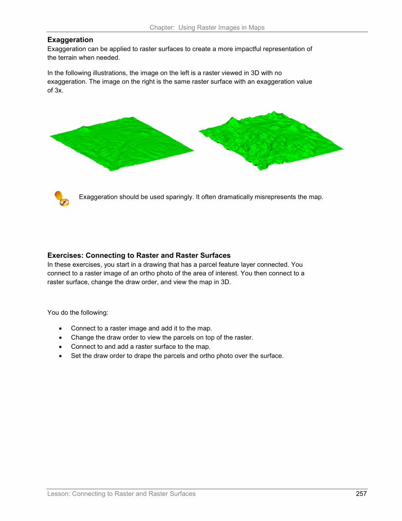
Exaggeration Exaggeration can be applied to raster surfaces to create a more impactful representation of the terrain when needed.

In the following illustrations, the image on the left is a raster viewed in 3D with no exaggeration. The image on the right is the same raster surface with an exaggeration value of 3x.

Exercises: Connecting to Raster and Raster Surfaces In these exercises, you start in a drawing that has a parcel feature layer connected. You connect to a raster image of an ortho photo of the area of interest. You then connect to a raster surface, change the draw order, and view the map in 3D.

You do the following:

• Connect to a raster image and add it to the map. • Change the draw order to view the parcels on top of the raster. • Connect to and add a raster surface to the map. • Set the draw order to drape the parcels and ortho photo over the surface.

Exaggeration should be used sparingly. It often dramatically misrepresents the map.



7.3.1 Connecting to an Aerial Photo


1. Open the drawing Connect to Raster.dwg from the Chapter 07 folder.

In the first series of steps, you connect to the raster image and add it to the map.

2. If the Task Pane is not visible, at the command line enter: Command: MAPWSPACE.

3. At the command line, enter ON to display the Task Pane, which includes the Display Manager.

4. In the Display Manager, confirm that the Groups button is selected.

5. In the Display Manager, click the Data button, and then select ⇒ Connect to Data… .

The Data Connect palette opens. Here you can select from many different data providers or sources. In this exercise you will be connecting to a raster image file.

6. From the Data Connections by Provider list, select Add Raster Image or Surface Connection.

7. Change the Connection name: to Ortho.

8. Click the file button and browse to: C:\A Practical Guide\GIS in Civil 3D 2018\Chapter 07, and select Aerial.tif.

9. Click <<Connect>>.



10. Click <<Add to Map>>.

11. Close the Data Connect palette.

Notice the feature layer Aerial now appears in the Display Manager. A layer in the Display Manager is different than an AutoCAD layer; it is the name of a data source and where you manage its properties.

Notice the aerial photo is on top of the parcels.

12. In the Display Manager, select the Draw Order button.

The list of feature layers is displayed in the current draw order. The order these are listed in matches the feature layers in the drawing.

13. Drag the Parcels feature layer above the Aerial layer.

The first time you change the sequence of the Display Map Draw Order list in a drawing, an alert is displayed, informing you that the Draw Order list will now control the visual display of feature layers.

14. Click Continue action and allow Draw Order to control layer position from now on.



15. Zoom into the map to view the image with the parcels overlaid.

16. Save the drawing for use in the next exercise.

7.3.2 Connecting to a Raster Surface

In this exercise you connect to and add to the map an elevation enabled raster, or raster surface. Once the surface raster is added to the map, you change the draw order, and view the map in 3D. Any feature layer that is on top of the surface will automatically drapes over the surface.

1. Continue working in Connect to Raster.dwg from the previous exercise.

If you did not complete the previous exercise you can open the drawing Connect to Surface.dwg.

2. Connect to a Raster Surface. Repeat Steps 5-11 from the previous exercise using the following information:

• For the Connection Name enter Elevation • Connect to the file Existing Ground.dem in the Chapter 07 folder

3. In the Display Manager, select Draw Order.

The list of feature layers is displayed in the current draw order. The order these are listed in matches the feature layers in the drawing.

4. Drag the feature layers to match the following order:

o Parcels o Aerial o Existing Ground

To view the Parcels and Aerial features draped over the Existing Ground DEM feature, you need to switch the drawing editor from 2D to 3D views. The tools to switch views reside on the Map Status Bar. In the standard, out-of-the-box installation of Civil 3D, this status bar is not displayed by default. The display of the Map Status Bar is controlled by a system variable.

5. Enter MAPSTATUSBAR on the Command Line, and select <Show>.

The Drawing Status Bar now shows additional tools for some AutoCAD Map 3D functions, such as 2D / 3D Viewing, Vertical Exaggeration, Coordinate Systems and View Scale.



6. In the Drawing Status Bar, click the 3D icon.

The drawing is displayed in 3D.

7. In the Status bar, for Vertical Exaggeration, select 2x.

Note: It might take a few moments to optimize the layer.

8. Zoom into the drawing to view how the raster and parcels are draped over the surface raster.

9. Experiment with various Vertical Exaggeration values and 3D viewing angles.

10. In the Display Manager, turn the Aerial image off, and notice how the vector data in the Parcels layer are draped over the surface.

NOTE: Be careful when applying Vertical Exaggeration, and use it sparingly. While it can help visualize terrain in relatively flat areas, it can dramatically misrepresent actual conditions.

Lesson Review In these exercises you integrated three different sources of data. Vector based parcels, an ortho photo, and a surface. Together, these sources of data were combined to view how the parcels and the image drape over the existing ground terrain.

466

467

Index

3D Modeling Workspace 8 3D Navigation 282 Add Data to a Map 218 Adding New Features 316 Altering Properties 390 Anchors 36 Angle Data 25 Annotation Blocks 118 Annotation Template 118 Attach Object Data 59, 66, 69 Attribute Data 52, 53 AutoCAD Attach 244 AutoCAD Options 9 AutoCommit 90 Automatic Check In 314 Automatic Checkout 314 AutoSave 9 Best Route 433 Bitonal 242 Block Attributes 55 Bulk Copy 342 Cancelling Checkout 315 Capture Area 255 Centroid 422 Check-In/Checkout 314 Civil 3D Workspace 8 Classifying Existing Objects 155 Clustered Nodes 35, 416 COGO Inquiry 24 Command Line 10 Compound Queries 368 Connecting to ODBC 231 Connecting to Raster 261 Constraints 334 Contextual Ribbons 5 Contours 285 Convert Coordinate Systems 407 Coordinate Conversion 259 Coordinate Geometry 24 Coordinate System 17, 167, 216, 234, 405 Coordinate System Grid 458 Coordinate Tracker 18 Correlation Files 243 Create scale ranges 293 Creating New Classified Objects 160 Creating New Features 315 Crossing Objects 35, 416 Current Drawings 353 Data Panel 401 Data Queries 382 Data Source 85 Data Source Name 234 Data Table 225 Data Table Tools 226 Data View 89

Datums 15 Define Object Data 59 Digital Elevation Model 257, 281 Display Manager 6 Drafting & Annotation Workspace 8 Drafting Settings 9 Draping 260, 284 Draw Order 227, 250 Drawing Cleanup 415 Drawing Locks 357 Drive Aliases 354 Duplicate Objects 35 Dynamic Annotation 116 Edit Feature Attributes 313 Edit Feature Geometry 313 Edit Object Data 59, 75, 76, 78 Editing Attributes 315 Editing Existing Features 316 Editing Object Data Tables 79 Editing Transaction Model 397 Error Markers 425 Export file types 182 Export Process 184 Exporting 181 Exporting Civil 3D Objects 206 Expression Builder 307, 308 External Data Sources 53 External Databases 84 Feature Class 216 Feature Filters 306 Feature Joins 323 Feature Layer 217, 224 Feature Layer Selectivity 227 Feature Queries 306 Feature Source 210, 213 Feature Source Connect 214, 245 Feature Styles 268 Feature Thematic Maps 297 Filter to Select 309 Flood Trace 433 Generating Links 86, 98, 100, 102 GIS Contours 192 Global Coordinate Systems 15 Grey Scale 243 Hillshading 283 Image Behavior 250 Image Correlation 245 Image Frames 250 Image Insert 245 Import Attributes 167 Import Coordinate Systems 167 Import Geometry 167 Import Interface 168 Import Spatial Filters 167 Inserting Dynamic Annotation 123

468

Joins 322 Layout Elements 447 Legend 447 Line Feature Styles 272 Link Template 85, 98, 100, 101 Linking External Databases 85 Links 413, 422 Location Queries 363, 366 Manually Link 102 Map Book Dialog 463 Map Book Template 461 Map Books 445, 446 Map Explorer 6, 336 Map Status Bar 264 Network Analysis 432 Network Topologies 412 Nodes 413, 422 North Arrow 448 Object Class Objects 161 Object Classes 156 Object Classification 141, 142, 160 Object Classification Definition File 143 Object Data 54, 57, 67, 167, 383 Objects 211 ODBC 231 Online Map 254 Open Data Base Connectivity 233 Pipe Network 192 Planning & Analysis Workspace 8 Point Feature Styles 271 Polygon Feature Styles 272 Polygon Overlay 434 Polygon Topologies 421 Projection 15 Properties Palette 76 Property Alteration 392 Property Queries 363, 367 Pseudo Nodes 35 Quick View 355 Ranges and Styles 291 Raster 241, 242, 257 Raster Feature Layers 260 Raster Feature Source 258 Raster Metadata 244

Raster Surface 243, 259 Raster Surface Styles 282 Raster Surface Themes 284 Raster Surfaces 257 reference grid 449 Reference Management 250 Reference System 449 Refresh Annotation 119 Relational Data Base Management Systems 213 Ribbon 4, 225 Save-Back 396 Save-Back Options 399 Saved Queries 369 Scale Bar 448 Scale Dependent Styles 289 Scale Ranges 270 Schema 343 Schema Editor 336 Shortest Path 432 Source Drawings 352 SQL Queries 383 Style Editor 268 Style Editor Palette 270 Style Scale Ranges 268 Styles 270 Stylize Raster Surfaces 281 Stylizing features 268 Surface 192 Surface Exaggeration 261, 282 Task Pane 5, 226, 356 Theme Feature Labels 299 Theme Legend Labels 299 Theme Ramps 299 Themes 296, 391 Tolerance 36 Topology Analysis 431 Topology Object Data 414 UDL file 85 Update Annotation 119 User Interface 1 Validating Standards 153, 334, 337, 391 Vector Objects 242 Viewing Linked Data 103 Workspaces 8

Documents

A Practical Guide to GIS in AutoCAD Civil 3D...iv A Practical Guide to GIS in AutoCAD Civil 3D 2018 Introduction Congratulations on choosing this course to help you learn how to use