A

 

 

APPLICA

D

Pr

ATION O

SURFAC

DissertatiE

resident: PrSupe

Me

OF AQUA

CE-GROU

Mar

ion to obnvironm

rof. José Maervisor: Prof

Co‐supeembers: Pro

Dr

J

ATIC BIO

UNDWAT

 

ryam Shap

btain themental En

Jury 

anuel de Saf. Luis Filipeervisor: Dr. Aof.Luis Cancr. Tibor Stig

June 2012

DIVERSI

TER ECO

pouri 

e Master ngineerin

ldanha Gone Tavares RiAna Silva ela de Fonster 

2 

TY TO M

OTONES

Degree ng 

nçalves Matbeiro 

seca 

MONITOR

S

in 

tos 

1 

R

2  

Acknowledgment: 

When I started to investigate for this work I knew very little in this subject. After two years working with

a group of specialist in this filed I end up learning so many things. I am grateful for all the support and

help that I received from my professors, friends and family.

First I would like to thank my previous professor and my dear friend Paula Tavares who initiated this

work and taught me many things in this field. She kindly passed me her valuable experiment and

knowledge and I am so happy that I started my first steps with her.

I do like to thank Professor Luis Ribeiro for accepting the supervision of this thesis. He never

hesitated to help me when I needed and gave me the possibility to work on a topic that I really liked.

I also like to thank Dr. Ana Silva for her valuable advices during the work. She was always available

and helpful specially for running the Primer software and fundamental revision of the thesis. This work

has been done under her supervision in all the steps.

I truly want to thank Professor Luis Fonseca, for teaching me great experiment in the field, laboratory

and specially identification of fauna. I will always be grateful for his generous welcome in Algarve

University, the full integration in the Lab and all the support that he provided me.

I would like to thank Dr. Paula Chainho for hosting me in the Oceanographic Centre in Lisbon

University. I always enjoyed from discussion with her and I am so grateful for her helpful advice for

writing this thesis.

I appreciate my dear friends help in Benthic Ecology Laboratory, in Lisbon University. They assisted

me identifying the benthic fauna and they were always keen to pass their knowledge.

I would like to thank Dear Margarida Machado for her sincere help in the identification of benthic

fauna. I enjoyed spending time with her and working in her laboratory in Algarve University. Without

her help it was not possible to finish the identification.

3  

Dr. Sanda Lepure, and their group in Imdea Centre in Universidad de Alcalá in Spain. Sanda had

given me great hand in identification of groundwater fauna. I am more than grateful for her help in the

laboratory and valuable scientific discussion that made me motivated to continue working on this field.

I am thankful to Dr.Tibor Stigter, for his company in the field and passing great information on the

geology and hydrogeology aspects of the study area.  

 

Geosystem center (CVRM) is appreciated for having hosted this study. In particular, the financial

support by CLIMWAT project facilitated the samplings and field trips.

 

I do like to thank my dear friends from CVRM and master degree study to make these two years such

a memorable and joyful experiment. I want to thank my friends out of university for their sweet and

warm encouragements and being with me every moment of my life.

My last but not least thanks are for my family, my dear parents, my brothers and my sister to give me

the courage to travel abroad and expend my knowledge in a global experiment. I want to thank Vahid

my dearest friend, company and husband that has been always push me through the difficult moment

of my scientific life. The accomplishment of this work owes to you for giving me your brilliant idea,

warmest company and kindest help. 

 

 

                                                                                                                             Maryam Shapouri, June 2012 

 

 

 

 

 

 

 

 

 

4  

Abstract

This study follows two experiments with two different objectives. The first experiment aimed to

characterise the estuarine benthic community along a salinity gradient reflecting the conditions of

groundwater dependent ecosystems. The second experiment aimed to examine the sensitivity of

stygofauna to variation in groundwater salinity/conductivity accessed through wells. In the first

experiment, the spatial and temporal differences in the structure and composition of benthic

invertebrates were studied at a branching channel of the main estuarine channel of Arade river in

south of Portugal, which receives significant groundwater input and is also influence by semi diurnal

tides from the Arade estuary. Benthic macroinvertebrates were sampled at the end of the wet and dry

periods in 2009, along the salinity gradient created by the groundwater entrance in the channel.

Physico-chemical variables were measured to determine their association in the benthic fauna

distribution. Results indicated that the abundance of species Isopode Cyathura carinata and the

Polychaeta Heteromastus filiformis varied significantly with the salinity gradient created by the

groundwater discharge into the estuarine habitat and with sampling time. The Polychaeta were more

abundant at the end of dry season than wet season, and also are more abundant at the points of high

salinity, suggesting their tendency for being more associated to saline water. However, the

Polychaeta Hediste diversicolor and Alkmaria romijni were more abundant in areas of lower salinity

and at the end of the wet season. Some taxa such as Oligochaeta did not display any orientated

distribution pattern as a response to both period and location factors, being abundant at the end of

wet season and simultaneously at the saline water points. The Polychaeta Alkmaria romijni was the

dominant species and ubiquitous throughout sampling stations .Among environmental variables,

salinity was the most explaining abiotic variable of the community distribution pattern.

In the second experiment, six wells were selected for sampling in which four of them were more

associated to salinization risk as they are located close to Arade estuary, whereas the remaining wells

are relatively far from the sea. Wells fauna was sampled with the use of a phreatobiological net and

well sediment sampling device developed for the present study (WSSD). Wells were grouped into two

categories based on their salinity. A total of 612 number of individual were collected and 19 species.

were identified. For all the 6 wells a total of 240 species were identified as true groundwater fauna.

Identification to species level is still on going. The Order Cyclopodia dominated in all 6 wells with

relatively high diversity. There was an apparent relationship between salinity level of well water and

stygofauna presence. The species Eucyclops speratus, Eucyclops hadjebensis, Megacyclops viridis

and Acanthocyclops sensitivus were particularly associated with low salinity conditions, hence being

potential indicators for saline intrusion if their abundances decrease greatly. Conversely, the taxa

Halicyclops sp. was identified as a possible indicator of high salinity conditions. The greatest diversity

and highest abundance were found in the lowest salinity condition. The comparison between the two

sampling methods indicated that the Phreatobiological net is more effective in gathering

representative samples, particularly from Cyclopodia which are generally good swimmers, while the

WSSD net is more suitable to have sample groups adapted to benthic life such as Harpacticoids and

Ostracods.

5  

Keywords: Benthic fauna, salinity gradient, groundwater habitat interface, climatic and human

pressures 

Resumo

Este trabalho é composto por duas grandes linhas de investigação. A 1ª teve como objectivo

caracterizar a comunidade estuarina bentónica ao longo de um gradiente salino que recria as

condições de um ecossistema dependente de águas subterrâneas. A 2ª grande temática teve com

objectivo examinar a sensibilidade da stygofauna a variações na salinidade/condutividade eléctrica

através de amostragens em poços artesanais. Na experiência estuarina, as diferenças na estrutura e

composição de invertebrados bentónicos foram estudadas no canal adjacente ao canal principal do

estuário do Arade no Sul de Portugal. Este recebe uma contribuição importante e directa de água

subterrânea e simultaneamente é influenciado por marés semi-diurnas do estuário. Os

macroinvertebrados bentónicos foram amostrados no final dos períodos seco e húmido em 2009, ao

longo do gradiente salino criado pela entrada de água subterrânea no canal. Variáveis físico-

químicas foram medidas para determinar a sua associação à distribuição da fauna bentónica. Os

resultados indicam que a abundância do isópode Cyathura carinata e do polychaeta Heteromastus

filiformis variou significativamente com o gradiente de salinidade criado pela descarga de água

subterrânea para o habitat estuarino e com o período de amostragem. Os poliquetas foram mais

abundantes no final do período seco do que no húmido, e nos locais de amostragem de maior

salinidade, sugerindo uma associação com águas mais salinas. No entanto, os poliquetas Hediste

diversicolor e Alkmaria romijni foram mais abundantes em áreas de menor salinidade e no final da

época húmida. Alguns taxa como sejam os Oligoquetas não revelaram nenhuma tendência no seu

padrão de distribuição espacial ou temporal. O poliqueta A. romijni foi a espécie dominante e

distribuída por todas as estações de amostragem. De entre as vaiáveis ambientais medidas, a

salinidade foi a que mais contribuiu para explicar o padrão de distribuição das comunidades.

Na segunda linha de investigação, 6 poços artesanais foram seleccionados na mesma área de

estudo, em que 4 deles estão associados a risco de salinização por se encontrarem perto do estuário

do ri Arade, enquanto que os outros estão relativamente longe do mar. A fauna existente no fundo

dos poços foi amostrada com uma rede freatobiológica e com um aparelho de amostragem em poços

desenvolvido para o presente estudo (WSSD. Os poços foram agrupados em 2 categorias com base

na salinidade da sua água. No total, foram amostrados nos poços 612 organismos que representam

19 espécies. A ordem Cyclopodia foi a dominante em todos os poços com uma relativamente

elevada diversidade. Foi verificada uma aparente relação entre o nível de salinidade da água do poço

e a presença de stygofauna. As espécies Eucyclops speratus, Eucyclops hadjebensis, Megacyclops

viridis e Acanthocyclops sensitivus foram encontradas associadas a condições de reduzida

salinidade, sendo potenciais indicadoras de intrusão salina costeira se a sua abundância decrescer

acentuadamente. Por oposição, o taxa Halicyclops sp. foi identificado como um potencial indicador

de condições de mais elevada salinidade. A maior abundância e diversidade foram encontradas na

salinidade mais baixa. A comparação entre os dois métodos de amostragem indicou que a rede

6  

freatobiológica é mais eficaz na recolha de amostras representativas, particularmente de Cyclopoids

que são geralmente bons nadadores, enquanto que o WSSD é mais adequado para amostragem de

grupos adaptados a vida bentónica como sejam os harpaticóides e os ostracódes.

Palavras de chaves: Fauna bentica, gradiente de salinidade,  interface de habitat de águas

subterrâneas , Pressões humanas e climáticas 

 

 

 

 

 

 

 

 

 

 

 

 

 

 

 

 

 

 

 

 

 

 

 

 

7  

ContentsChapter 1 1.1  Introduction ................................................................................................................... 11 1.2  State of art ..................................................................................................................... 14 1.2.1  Groundwater/surface-water ecotones (transitional zone) .......................................... 14 1.2.1.1  Concept of groundwater, water table and flow system ......................................... 16 1.2.1.2  Recharge -discharge behaviour of coastal aquifers ............................................... 17 1.2.1.3  Groundwater dependent Ecosystems ..................................................................... 18 1.2.1.4  GW-surface water interaction and salinity variation in the wetland ..................... 19 1.2.2  Climate change and groundwater surface water variability ...................................... 20 1.2.2.1  Climate change impact and aquifer vulnerability in the Mediterranean area (study area): ……………………………………………………………………………………21 1.2.2.2  Biological response to climate change on aquatic ecosystems .............................. 22 1.2.3  Monitoring of water resources and dependent ecosystems using bioindicators ....... 22 1.2.3.1  Ecological assessment and environmental policies “The Water Framework Directive”…………………………………………………………………………………… 24 1.2.3.2  Benthic Macroinvertebrates as an indicators of ecological status ......................... 24 1.2.3.2.1  Benthic community response to salinity gradients in estuaries ............................. 25 1.2.3.3  Seasonal and spatial patterns of benthic invertebrates .......................................... 27 Chapter 2 2.1  Abstract ......................................................................................................................... 29 2.2  Introduction ................................................................................................................... 30 2.3  Methods......................................................................................................................... 32 2.3.1  Study area .................................................................................................................. 32 2.3.1.1  Hydrology and hydrogeology: ............................................................................... 33 2.3.1.2  Land use ................................................................................................................. 33 2.3.2  Sampling design ........................................................................................................ 33 2.3.2.1  Environmental variables measurement:................................................................. 35 2.3.3  Data analysis ............................................................................................................. 37 2.3.3.1  Spatio-Temporal variation ..................................................................................... 37 2.3.3.2  Relationships between environmental and biological variables ............................ 37 2.4  Results ........................................................................................................................... 38 2.4.1  Benthic macrofauna general characterization ........................................................... 38 2.4.2  Species distribution ................................................................................................... 38 2.4.3  Species contribution for spatial and temporal differences ........................................ 42 2.4.4  Environmental variables ............................................................................................ 43 2.4.5  Abiotic variables contribution for community distribution ....................................... 44 2.5  Discussion ..................................................................................................................... 46 2.5.1  Groundwater availability and community predictions .............................................. 46 2.5.2  Variation in groundwater discharge and food-web implications .............................. 47 Chapter 3 3.1  Abstract ......................................................................................................................... 50 3.2  Introduction ................................................................................................................... 51 3.3  Methods......................................................................................................................... 54 3.3.1  Study area: ................................................................................................................. 54 3.3.2  Field abiotic measurements ....................................................................................... 54 3.3.3  Sampling design: ....................................................................................................... 55 3.3.4  Wells fauna assessment ............................................................................................. 57 3.4  Preliminary Results and interpretation .......................................................................... 57 

8  

3.4.1  Fauna general characterization .................................................................................. 57 3.4.2  Species distribution ................................................................................................... 60 3.4.3  Sampling device comparison .................................................................................... 61 Chapter 4 4.1  Main Conclusions and future works ............................................................................. 64  

Bibliography ............................................................................................................................ 66  

IndexofFigures 

Figure 1.1- GW-SW interact throughout all landscapes K; Karst; M: Mountain, R: riverine (small); C: Costal; G: Glacial; V: riverine (large)…………………………………………………15

Figure 1.2- Location of the saturated and unsaturated zones in relation to the water table and processes involved in the water movements (USCS)……………………………………...17

Figure 1.3- Remane curve (after Remane, 1934), showing quantitative relations between freshwater, brackish and marine invertebrate species…………………………………………26

Figure 2.1-The enlarged map the Algarve province and the main water courses (blue) and corresponding catchment area (orange line). The main area of Querença-Silves aquifer is shown by light blue area……………………………………………………………………………32

Figure 2.2-Sediment sampling points. First location on the right side of the bottom image corresponds to the GW discharge point. The salinity gradient is also marked by colours from the lowest point (blue) to the highest point (red)…………………………………………………34

Figure 2.3- Specific sampling locations. Point C refers to the location of GW discharge and Point E is located in the connection of the branching channel to the main estuary canal…..35

Figure 2.4- Estômbar channel , a branching channel of the Arade estuary at low tide(A), and the location of sampling points A,B, and C in low tide(B); the Estômbar channel in high tide(C) and location of groundwater input at high tide(D)……………………………………… 36

Figure 2.5-MDS ordination of fauna sediment samples collected at the end of the dry and wet times, in the distance gradient originating at the location of groundwater input (A -E)…39

Figure 2.6- Temporal variations on the densities of taxa that contributed the most on the dissimilarities between periods…………………………………………………………………….40

Figure 2.7- dbRDA ordination of the sample variation during wet (Wet) and Dry (Dry) season and in five locations (A, B, C, D, E) for the abundance of species ……..……………………. 42

Figure 2.8- Variation of water level, electrical conductivity (EC) and temperature at the location of groundwater discharge into the Estômbar channel of the Arade estuary; also indicated are the tidal fluctuations measured in Lagos, located 20 km towards the west…..43

9  

Figure 2.9- PCO analysis of biota distribution accordingly to sampling points with overlaid vectors of environmental variables contribution to biota distribution…………………………..45

Figure 3.1- Location of the inventoried wells. Wells number 2,3, 22,23,25 and 26 were sampled………………………………………………………………………………………………54

Figure 3.2- Phreatobiological net and its deployment………………………………………… 55

Figure3.3- Well Sediment Sampling Device and its deployment………………………………56

Figure3.4-some representive Stygofauna, sequently from left up to right down: gamarus pulex/Eucyclops serrulatus serrulatus / Cypridopsis vidua/ Harpacticoida/ Macrocyclops albidus/ Eucyclops / Megacyclops Viridis/ Gammarus pulex…………………………………..60

Figure 3.5-MDS ordination of wells fauna samples collected from 6 different wells (Q1-Q6), with three replicate from each well (R1-R3)grouped into two groups of salinity categories (H: high and L:low salinities)…………………………………………………………………………. 60

IndexofTablesTable 2.1- Permanova analysis of the sediment fauna for factors Period (dry and wet) and Location (A-E). The number of permutations used was 9999 (Ti=period, Lo=Location)……38

Table 2.2- SIMPER analysis identifying the species that contributed the most for differences between seasons for all locations…………………………………………………………………39

Table 2.3. SIMPER analysis identifying the taxa that contributed the most to differences from point D to the freshwater point (C )…………………………………………………………41

Table 2.4- SIMPER analysis identifying the species that contributed the most for dissimilarities between point D and point B……………………………………………………...41

Table2.5. Biota and environmental matching according to the BEST modelling…… …..…..44

Table3.1-. Wells abiotic and morphologic characteristics. Wells numbers 1, 2,3,4,5 and 6 refers to wells illustrated in “figure 1” by codes 2, 3, 22, 23, 2 and 26 respectively. n.a.-not available……………………………………………………………………………………………...54

Table 3.2- Identified species of Cyclopodia, Ostracod, Amphipod and Copepod sampled rom wells. Shaded cells represent absence and unshaded cells represent a taxa absence…….57

Table 3.3- Taxa abundance sampled by Phreatobiological net and WSSD…………………60

Table 3.4- SIMPER analysis identifying the species that contributed the most for differences between wells with high and low salinities………………………………………………………..61

Table3.5- Taxa abundance sampled by Phreatobiological net and WSSD……………….…61

 

 

10  

Chapter 1: General introduction and state of art  

 

 

 

 

 

 

 

 

 

 

 

 

 

 

 

 

 

 

 

 

 

11  

1.1 Introduction 

Habitats located at groundwater–surface water interfaces, i.e. transition zones, are considered to be

spatially and temporally dynamic (e.g. Malard et al., 2003; Bork et al., 2009). These transition zones

often display complex temporal and spatial variation on benthic macroinvertebrates community

(Rundle et al., 1998; Bork et al., 2009). Ecotones are characterized as dynamic components of a

landscape, providing habitat for many transient organisms that explore highly shifting environments

(Senft, 2009). Transitional zones in the estuary may have lower diversity in terms of benthic

communities when compared to freshwater and higher salinity areas, due to natural stress (e.g.

salinity variation)(Medeiros et al., 2011). The conservation of these habitats offers some challenges

because ecotones may appear to have lower diversity if they undergo through frequent or intense

disturbance events (Chapman, 1960 and Senft, 2009). Groundwater and surface water are connected

in a hydrological continuum and often originate transient zones, which provide refuge conditions, sites

of high biodiversity and habitat for the macrofauna, microbial production, and energy transfer

(Tomassoni, 2000). Climate is an important factor affecting water quality and availability in the

interaction zone. The change in the precipitation and temperature future regimes, induced by climate

change, will lead to change in the runoff, aquifer recharge, flood and drought frequency and

magnitude, as well as in the quality of the water resources (Santos et al., 2002; Ajami et al., 2008).

Groundwater resources are currently under severe threat due to Human usage and pollution

(Danielopol et al., 2003). As depletion of superficial water occurs and because climate change effects

are predicted to greatly enhance the demand on usable freshwater, groundwater is thought to be the

primary provider meeting the Human multiple demands on this limited resource (Danielopol et al.,

2003; Santos et al., 2002). Substantial aquifer exploitation threatens the wetlands that are also

groundwater dependent ecosystems (GDEs) (Boulton, 2009; Humphreys, 2009). In the south regions

of Portugal, where the present study was made, groundwater represents 60% of drinking water and

fulfils 80% of agricultural demand (Stigter et al., 2009). This demand is likely to be enhanced in this

geographical area as a result of global warming (Santos et al., 2002).

The benthic invertebrate community has been considered a very useful tool to monitor and assess the

Human induced impact on the aquatic environment due to their measurable response to natural shifts

and anthropogenic impacts (Chainho, 2008). Benthonic macroinvertebrates are identified by the

Water Framework Directive (WFD) as useful bioindicators of the ecological status of water bodies

(2000/60/CE) (Sandin and Hering, 2004; Borja et al., 2009, Silva et al., 2012). Many species of the

benthic community such as Polychaeta but not amphipods, show reduced mobility and in case of

contamination, they will be exposed to the stress for longer time periods, hence therefore they can

reflect also the effects of long term environmental disturbances (Chainho, 2008). In the context of

habitat management, biological monitoring methods present several advantages: biological response

reflects the conjugated action of environmental conditions and make the impact easily detected,

evaluate factors not directly measurable such as biological complexity and ecological value and, no

expensive laboratorial chemical analysis are required (Ambrogi and Forni, 2004, Silva et al., 2012).

Some biological characteristics of benthic species have to be taken into account when interpreting

12  

results of benthic community as a whole. Benthic fauna show high spatial heterogeneity related to

their tolerance to the influence of different environmental factors such as salinity, sediment type,

temperature, etc. Moreover, invertebrate communities also show important temporal variations related

to seasonal and interannual variation. Part of the seasonal fluctuation is associated with their

biological cycle due to recruitment processes that occur during spring and autumn for most species,

but also due the control of extreme climate event such as low temperatures, floods and droughts

(Alden et al., 1997; Attrill and Power, 2000; Salen-Picard and Arlhac, 2002; Chainho, 2008).

Moreover the organisms living within the shallow groundwater zone can serve as indicators of the

quality of the groundwater resource, particularly at the interaction and influence area of the surface

water systems (Claret et al. 1999). In fact, groundwater fauna reflect structural conditions of their

habitat such as hydraulic conductivity, heterogeneity of habitats in an aquifer and provide information

on surface/subsurface hydrological exchanges (Danielopol et al., 2007). Therefore, the relative

presence or absence of different communities or populations of organisms may reflect the impact of

changes in water quality, in similarity with the bio indicator function that many surface taxa display.

The CLIMWAT project aimed at evaluating the climate change impacts on the Querença-Silves

aquifer, which is a costal aquifer with dependent ecosystems , and one of eight transnational

research projects funded under the CIRCLE-MED network (Stigter, 2011). Querença-Silves was the

aquifer studied in the present thesis which was developed within the project. Different climate

scenarios were used to predict the future climate change impact on aquifer net recharge and

consequently the output to GDEs and water quality condition in different wells. Results from the

project indicated a significant decrease in recharge in the present study area for the future years. The

models calculated in the project, predict a significant increase in the mean temperature for future

years and, consequently it is expected an increase groundwater demand for crop cultures. Due to

increased extraction of aquifer water and less recharge flow into the aquifer, an overall decreasing

trend of groundwater levels is foreseen, which is likely to reduce the groundwater outflow into coastal

wetlands, threatening the ecosystem stability. Climate change has the potential to greatly influence

interface or border aquatic habitats such as estuaries and wetlands that are dependent on

groundwater, by altering environmental variables such as temperature, salinity, etc. (Bates et al

2008). The combined effect of prolonged and large extractions from the aquifer and reduced recharge

in coastal areas can lead to seawater intrusion, a serious problem worldwide, including the

Mediterranean countries.

This study follows two experiments with different objectives and study site. The first experiment was

made in an estuarine branch which receives groundwater from the coastal aquifer and brackish tidal

water originated from the main estuary channel. In fact, the branching channel was located

approximately half-way between the river and sea points of the estuary. It represents an interface

area between the main estuary channel and a point of considerable groundwater direct discharge

from the Querença-Silves aquifer into the estuary. This interface ecosystem is a perfect case study to

evaluate the estuarine benthic community response to changes in groundwater input from aquifers.

The main objective of the present study was to test the hypothesis of there being a relationship

between the distribution pattern of benthic estuarine taxa and the groundwater availability in the

13  

estuary. The present study also aimed to identify benthic estuarine taxonomic groups and/or species

which can potentially be monitored to ecological impacts of changes in groundwater discharge. It was

expected that benthic communities responded in presence, abundance and potentially in population

structure, to the gradient in salinity originated by the freshwater input into the estuary, due to

discriminating salinity tolerances of organisms and species.

The second experiment aimed to examine the sensitivity of stygofauna to variation in groundwater

salinity/conductivity accessed through wells. Assessing the biodiversity and abundance response of

groundwater fauna sampled in aquifers of differing groundwater characteristics allows evaluating

impacts such as seawater intrusion on the vulnerable groundwater ecosystem. This experiment also

aimed to provide ground breaking biological data to integrate the use and conservation of

groundwater dependent fauna into aquifer management. Six wells were selected for sampling in

which four of them were more associated to salinization risk as they are located close to Arade

estuary, whereas the other two wells are relatively far from the sea. Wells fauna was sampled with the

use of a phreatobiological net developed for large diameter wells, as well as a well sediment sampling

device developed for the present study (WSSD).

This thesis was divided in four different chapters as it follows:

Chapter 1 is a general introduction that summarises the two experiments with their respective

objectives. It also contains the state of art in which some key themes of the study will be

explained by details.

Chapter 2 consists of an experiment that identifies Spacio-tempral variation of benthic

communities in GDEs influenced by climate change. Chapter 3 consists of second experiment in which stygofauna were used for assessing

groundwater with different conductivity condition.

Some final remarks are presented in Chapter 4, integrating the results obtained in each

chapter and presenting the major conclusions of the study.

14  

1.2 Stateofart 

Freshwater ecosystems fed by groundwater or/and surface water, have been important sources for

the development of environmental monitoring programmes (De Pauw et al., 1992). The management

of the freshwater ecosystem needs to integrate the groundwater exploitation, as well as surface water

bodies and ecosystems. Wetlands are characterized by large land-water interfaces that regulate the

ecological status of ecosystems established there (Winter, 2003; Euliss et al., 2004). Wetlands that

are linked to aquifers also include surface-groundwater interfaces and are referred to as groundwater

dependent systems (GDEs). A wide range of disturbance sources including pollution may affect the

groundwater quality and availability (Danielopol et al., 2003). Climate change has direct impacts on

the availability, timing and variability of the water supply and demand, and is also related to the

significant consequences of these impacts on many sectors of our society. Bioindicators sensitive to

climate variability impacts on coastal waters (and ecosystems) quantify the impacts of climate change

on water quantity and quality. For this study, ecosystems have been studied with particular attention

for the ecotones where groundwater and surface water bodies interact. Assessing the bioindicators

representing different ecotones and trophic levels (e.g. invertebrates, vegetation and respective

predators) enables to integrate pollution effects at different spatial and time scales. Indicators of

ecosystem health improve the efficiency of ecosystem management such as that of southern

wetlands in Portugal, where climate changes are predicted to enhance eutrophication and droughts

effects. In a groundwater-brackish water ecosystem with high instability in environmental factors such

as salinity and conductivity, invertebrates are expected to respond, and therefore could be used as

potential important tools in the assessment and management of surface and groundwater availability

under different climate change scenarios and uses. The following review section analysis the current

knowledge of the role that groundwater–surface water (GW–SW) interactions play in the ecology of

arid/semi-arid wetlands, particularly those which are dependent on groundwater inputs. The key

themes of the review are as follows: (i) Groundwater/surface-water ecotones, (ii) Impact of climate

Change on water resources particularly in interaction zones and on the ecosystems depending on

groundwater input and, (iii) Application of biological indicators of climate change and anthropogenic

impact in the mentioned ecosystems.

1.2.1 Groundwater/surface‐waterecotones(transitionalzone)

Ground and surface waters are usually evaluated as separated water masses, but hydraulically they

are connected and the groundwater contacts and feeds all types of surface water aquatic habitats

such as lake, stream and wetland in different terrains from mountain to ocean (Fig.1.1) (Winte, 2000).

 

Figure 1.1

In the pr

water ty

measure

mixture.

with a h

2009). M

such as

changes

et al., 2

1‐ GW‐SW inter

resent study

ypes, such as

e the water

The transitio

high heteroge

Moreover, ch

s daily cycle

s, and long-t

2000). Unde

ract throughou

, the ecotone

s groundwat

type intera

on zone betw

eneity in spa

hemical and

es (e.g., tem

term climatic

erstanding th

ut all landscape

riverine (la

e concept re

ter/surface w

action since

ween surface

ace and time

biological pr

mperature a

c changes an

he interactio

es K; Karst; M: M

arge) (Winter e

efers to the tr

water and fre

many natur

e and ground

e (Boulton e

rocesses in t

nd transpira

nd events (s

n between

Mountain, R: ri

et al., 2000) 

ransition zon

eshwater/salt

ral and anth

dwater is cha

t al., 1998; M

this zone ope

ation), short-

uch as extre

groundwater

iverine (small);

ne between tw

twater. It is c

hropogenic a

aracterised b

Malard et al

erate at diffe

-term weath

eme weather

r and surfac

; C: Coastal; G: 

two water bo

considered d

activities aff

by dynamic g

., 2002; Bro

erent tempor

her events,

r events) (To

ce water ca

15 

Glacial; V: 

odies and

difficult to

fect their

gradients

ke et al.,

ral scales

seasonal

omassoni

an be an

16  

important tool for water resources management, aiming to preserve the ecosystem stability and

determine the migration pathways of contaminants (Winter et al., 2003). The movement of surface

and groundwater is controlled by a natural condition of an area such as climate, through the effects of

precipitation and evapotranspiration that affects the distribution of water to—and removal from—

landscapes. The precipitation distribution pattern is highly variable in space and, evaporation and

evapotranspiration also vary under different climatic conditions, often even showing differing patterns

in a relatively small spatial scale from forest to nearby urban area. The physiography of the area such

as land-surface form and geology are also parameters controlling the groundwater and surface water

movement (Winter et al., 2003). Therefore, it is necessary to understand the effects of physiography

and climate on surface water runoff and groundwater flow systems, taking into account the impact of

human activities on their functioning and thus, on ecotones management policies. The mixture of two

water bodies in an ecotone may have major impacts on the individual ecosystems, if major

environmental factors such as temperature, acidity or dissolved oxygen are altered (Winter et al.,

2003). Due to the water interchange between surface-groundwater bodies, any shifts or

contamination of one commonly affects the other one. Surface waters are more vulnerable to pollution

due to their easy accessibility for disposal of wastewaters. Both the natural processes, such as

precipitation inputs, erosion, weathering of crustal materials, as well as the anthropogenic influences

such as urban, industrial and agricultural activities and exploitation of water resources, determine the

quality of surface water in a region. In turn, groundwater recharge is currently and in the future

predicted to be altered as a result of climate change and anthropogenic impacts (Ajami, et al., 2008).

Transitional zones are also ecologically important because some surface and groundwater organisms

have a life stage dependent on this zone, hence being vulnerable to any habitat shift. Ecotones

established at surface/groundwater or fresh/saltwater interfaces are flexible to changes in water mass

fluxes and have intermediate biodiversity (Vervier et al., 1992), but less is known of the unique

species that permanently inhabit in the transition zone and many have not been described.

Ecologically, the ground-water/surface-water transition zone is an important ecosystem affecting

several trophic levels from microbes to fish (Bear et al., 1979).

1.2.1.1 Conceptofgroundwater,watertableandflowsystem 

Groundwater is found underground in the unsaturated and saturated zones. In the unsaturated zone,

the voids which represent the space between the soil grains are filled by air and water. The water

present in this zone does not have the potential to be easily used because it is not feasible to pump

this water from the wells, mostly due to capillary force holding the water into the soil. The “soil water

zone” occurs at the top of the unsaturated zone. This layer is typically crossed by voids created by

roots (live and decaying), animal and worm burrows, all which will increase the water infiltration into

the soil. Soil water is used by plants and goes back to atmosphere through their transpiration or

evaporation directly from the soil. On the contrary, the saturated zone is completely filled with water

and the water in this zone is referred as groundwater. The upper section of the saturated zone is

referred as water table (Fig.1.2) (Winter, 2000).

17  

Saturated ZoneBelow the water table

(Ground Water)

Capillary fringe

Soil zone

Un

satu

rate

d z

on

e

Recharge to water table Water table

Evaporanspiration

Precipitation

 

Figure 1.2‐ Location of the saturated and unsaturated zones in relation to the water table and processes involved in the water movements  

The water table meets the surface water at or near shorelines if the surface water body is connected

to groundwater systems. The depth to the water table is variable in different landscapes but is smaller

near permanent surface water bodies such as lake and wetlands. The water table configuration varies

seasonally because the recharge into the saturated zone is affected by the precipitation pattern that

also depends on seasons. The groundwater flow system can operate at the local, intermediate and

regional scales. The most dynamic and shallowest flow is the local flow and therefore more in

interchange with the surface flow. The deeper flow systems such as those at the regional and

intermediate scales reside longer underground and, are more in contact with subsurface material, so

that when they discharge into the surface water, it has augmented effect on the chemical

characteristics of the interaction zone. Three types of flow regime can be described for the GW–SW

ecotone, which occurs mostly in wetland ecosystems: (i) recharge: surface water penetrates into the

underlying aquifer; (ii) discharge: surface water gains water from the underlying aquifer; or (iii) flow-

through: the surface water gains water from the groundwater in some locations and loses it in others

(Winter, 2000).

1.2.1.2 Recharge‐dischargebehaviourofcoastalaquifers 

18  

The most dynamic boundary of great part of the groundwater flow systems is the water table. The

location of the water table changes continually in response to recharge and discharge from the

groundwater system (Winter, 2000). Changing meteorological conditions (e.g. precipitation) strongly

affect aquifer recharge, especially near the shoreline. The water table commonly intersects the

terrestrial surface at the shoreline, resulting in no unsaturated zone at this point. Because the water

table is near the surface adjacent to shoreline, the precipitation passes rapidly through a thin

unsaturated zone and recharges into the aquifer, potentially resulting in increased groundwater inflow

to surface water bodies. Transpiration by near-shore plants has the opposite effect, because plant

roots can penetrate into the saturated zone, allowing the plants to transpire water directly from the

groundwater system. The transpiration effect is very high in some areas whereby there is a

groundwater movement into the surface water during the night, and surface water discharge into

shallow groundwater during the day. These periodic changes in the direction of flow also can take

place on longer time scales such as, seasonally or annually. Recharge to the aquifer from

precipitation predominates during wet periods, and removal by transpiration predominates during dry

periods. As a result, the two processes—together with the geologic controls on seepage distribution—

can cause flow conditions at the beds of surface water bodies to be extremely variable. These

processes probably affect ecosystems depending on groundwater discharge more than other

ecosystems (Winter, 2000).

Costal and riverine wetlands have a relatively complex hydrologic pattern because they are subjected

to water level changes mostly due to tidal flow. The costal wetland is also likely to be affected by the

periodic tidal cycle, as well as the changes in water level due to seasonal changes in precipitation.

These combined changes, along with precipitation, evapotranspiration and surface-ground water

interactions, determine the water quality and availability in the wetland ecosystems. Among the

wetland, the present work focuses on coastal wetlands that depend on freshwater input mostly

originating from groundwater. These bordering wetlands ecosystems can more directly reflect the

consequences of any shifts in the aquifer dynamics (Day et al. 2008), constituting the so called

groundwater dependent ecosystems (GDEs). Shifts in the chemical and ecological status of these

GDEs may occur as a consequence of changes in groundwater availability and/or quality related to

climatic change effects (Danielopol et al., 2003; Eamus and Froend, 2006), hence affecting all

wetland biotic elements including vegetation, invertebrates, fish and birds.

1.2.1.3 GroundwaterdependentEcosystems 

Groundwater dependent ecosystems (GDEs) are ecosystems that require the input of groundwater to

maintain their ecological structure and function (Murray et al., 2003; Murray et al., 2006). One of the

GDEs forms is wetlands which can be dependent on groundwater for all or part of the year.

Groundwater is essential to many ecological communities as a connector, not just in the aquifer itself,

but within, across, and between surface waters and many terrestrial ecosystems (Boulton, 2009).

Increasing awareness of groundwater issues worldwide are creating more opportunities to understand

how groundwater and their GDEs respond to altered hydrological regimes. Indeed, groundwater

19  

resources have been threatened due to increased demands on groundwater for consumption,

industry and agriculture. These demands alter groundwater regimes of GDEs that have evolved over

millennia, resulting in the degradation of ecosystem health. As a consequence, the goods and

services (ecosystem services) that GDEs provide for humans, which include food production and

water purification, are at serious risk of being lost (Murray et al., 2003). Groundwater resource

managers commonly ask how much water can be taken from the aquifer while still maintaining a low

level of risk to GDEs. This requires quantified information on the relationship between groundwater

flux quality and pressure on biota and ecosystem processes of GDES (Eamus and Froend, 2006).

Groundwater exchange influencessurface ecology due to the multiple services it provides including

means of delivering oxygen and food to microbial and invertebrate communities. According to

Malcolm et al. year 2005 dissolved oxygen varies over very fine spatial scales in groundwater

exchange zones influencing salmon ecology. Thus, the areas of upwelling cool groundwater could

provide refugia for brown trout during summer (Hancock and Boulton, 2009). Ecologists have come to

recognise that many stream ecosystems in surface, subsurface, and lateral compartments which are

linked by hydrological exchanges, convey nutrients, organic matter, dissolved oxygen, and some

invertebrates among these zones (Boulton et al., 1997).

Therefore, declining groundwater quantity or quality and variation in groundwater-surface water

interaction will influence the ecological communities. The ecological, hydrological, and physical–

chemical links between groundwater, surface waters and associated ecosystems are seldom fully

understood even though true characterization and wise management will require a multidisciplinary

approach. This means biologists need to understand the importance of magnitude and timing of

groundwater flows for the system, integrated with hydrology background knowledge. For collaborative

research to improve our understanding of links between groundwater and ecosystems, it needs to

focus on spatial and temporal scales that are relevant to both the hydrogeological and the ecological

process being studied. Effective management of GDEs and their ecosystem services requires

prioritisation of the most valuable ecosystems, given that increasing human demands and limited time

and money prevent complete protection of all GDEs.

1.2.1.4 GW‐surfacewaterinteractionandsalinityvariationinthewetland

Precipitation is one of the most dominant sources of water in nearly all wetland systems, yet the

influence of the groundwater flow component into the ecosystem can be sufficient from an ecological

perspective to yield an entire new type of wetland. Influxes of groundwater to lakes, rivers, and

wetlands can change whole-system physical–chemical properties such as temperature and salinity,

and also influencing microenvironments and their ecological processes (Boulton, 2009). Infiltration of

water from surface aquatic ecosystems and rainfall can have a significant effect on aquifer ecology;

therefore whether the water is flowing into or out of an aquifer, or is moving from one part to another,

it is the extent and intensity of connectivity that often determines its importance to ecosystems.

Coastal wetlands receiving tidal brackish water and groundwater, can range in salinity from sea water

(>30,0) to freshwater (0-0.5) (Redeke,1935).Salinity varies according to freshwater discharge, thus

20  

there are many differences between estuaries with different climatic regimes. In arid/semi-arid

environments, such as in the south part of Portugal examined in the present study, rainfall is seasonal

and significantly less than the evaporation rate. Hence, groundwater discharge into surface wetlands

can be a major component of the water quality and salt balance, which are major determinants of

wetland ecology. In semi-arid regions, the salinity in wetlands environments varies naturally due to

high evaporative conditions, infrequent rainfall, groundwater inflows, and after rains or floods (Jolly et

al., 2008). As a result of the human activities, including changes in land use, surface water regulation

and water resource availability, wetlands in arid/semi-arid environments are now often experiencing

extended periods of high salinity (Jolly et al., 2008). For the present study, the location where the

groundwater flows into surface systems is located in a channel connected to an estuary. The surface

water body is brackish closer to the estuary while it is less saline closer to the groundwater discharge

area. The canal is influenced by tidal brackish water daily, hence even in the point where groundwater

discharges into the wetland, the influence of the brackish water is high. When the groundwater inflows

increase, due to raised groundwater levels originated by factors such as land use change and river

regulation, this may have a major influence on the ecology of a wetland and its surrounding areas. On

the contrary, if the groundwater input to the wetland decreases, a scenario predicted for the region

(CLIMWAT Results), it can be expected that the ecosystem may alter strongly in the point with more

freshwater input. There are many knowledge gaps, particularly related to time-series data on the

salinity tolerance/sensitivity of freshwater aquatic biota and riparian vegetation.

1.2.2 Climatechangeandgroundwatersurfacewatervariability 

It is expected that predicted global changes in temperature and precipitation will alter regional

climates and hydrologic regimes in most areas of the world. The change in the precipitation and

temperature regimes, induced by climate change, will lead to changes in the runoff, aquifer recharge,

flood and drought frequency and magnitude, as well as in the quality of the water resources in

Portugal (Santos et al., 2001). In assessing the impacts of climate change on water resources, most

research has been directed at forecasting the potential impacts to surface water hydrology. For

groundwater hydrology, large regional and coarse-resolution models have been used to determine the

sensitivity of groundwater systems to changes in critical input parameters, such as precipitation and

runoff ( York et al., 2002). Although the effect of temporal variability in surface waters is more visible,

groundwater recharge is likely to be altered as a result of climate change and anthropogenic impacts

(Ajami, et al., 2008), especially in areas where it is more sensitive to climate variability such as

Mediterranean areas. Groundwater resources in the studied area, south of Portugal, are under

increasing pressure due to large extraction rates for various water-consuming activities, particularly

agriculture (irrigation), public water supply (consumption) and industry. Among the aquatic

ecosystems, wetland systems are more vulnerable to changes in quantity and quality of their water

supply, and it is expected that climate change will have a pronounced effect on wetlands through

alterations in hydrological regimes with great global variability (Erwin, 2009). Many wetlands depend

on groundwater flux throughout annual and seasonal weather changes, which direct to couple change

21  

on hydrological system of both water bodies. Because wetlands water level variation has an impact

on the surface flow and groundwater recharge. Substantial aquifer exploitation threatens the wetlands

that constitute groundwater dependent ecosystems (GDEs), and in coastal areas it can lead to

seawater intrusion, a serious problem worldwide, including the Mediterranean countries (Stigter et al.,

2009). It should be noted that intensive and uncontrolled groundwater exploitation can have similar or

more severe impacts on aquifers and related ecosystems than climate change. A correct

implementation of future adaptation measures requires a more detailed insight into the way climate

change affects aquifer recharge and discharge patterns to mitigate the expected disturbance

1.2.2.1 ClimatechangeimpactandaquifervulnerabilityintheMediterraneanarea(studyarea):

 

Climate change is predicted to be very noticeable in the Mediterranean region, due to the magnitude

of expected changes in temperature and rainfall patterns (Giorgi, 2006). Aquifers located in these

regions (e.g. Querença-Silves) are expected to be affected by climate change, particularly in arid and

semi-arid regions where decreases in recharge can become very significant in the following decades

(e.g.,Santos et al. 2002, Giorgi 2006). The aquifers may be more vulnerable to climate change if they

are located in regions where many Human sectors depend on them for their water supply. Drought

and increased water demand for agricultural activity affects the availability of surface water and will

lead to increased groundwater usage. Portugal is characterized by its mild Mediterranean climate,

with well-known water vulnerability to climate fluctuation, namely to droughts and desertification in the

southern sector (Santos et al., 2002). Severe droughts have occurred in the study area namely during

the hydrological year of 1991/92 and also in 2005 (Barros et al., 1995; Stigter, 2011). Climate change

may particularly aggravate this problem in the Mediterranean region (e.g. Giorgi 2006), due to the

combined effect of rising sea levels and reduced recharge of aquifers associated with the expected

decrease in precipitation and average temperature increase. In the CLIMWAT project it was examined

the effect of climate change in the present case study. Climate scenarios were calculated using the

available scenarios from the ENSEMBLES project as a starting point .The data of temperature and

precipitation for years 1960-1990 or 1980-2010 were used as a reference period, and aquifer

recharge was calculated for 2020-2050 and 2069-2099. Results for the calibrated period and

predicted climate scenarios indicated that discharge from the Querença-Silves aquifer into the Arade

estuary are to decline and therefore, it is modelled an increase in probability of occurrence of

seawater intrusion and the drying out of groundwater dependent wetlands. Continued climate stress

would increase the frequency with which ecosystem thresholds would be exceeded, leading to

chronic water-quality changes (Murdoch et al., 2000; Loáiciga et al., 2000).

 

22  

1.2.2.2 Biologicalresponsetoclimatechangeonaquaticecosystems

Variability within abiotic processes influences ecosystem properties. Continued climate changes can

threaten a large number of unique biological systems (Smith et al., 2001). While ecosystems have

coevolved with these abiotic disturbances and biotic disturbances such as insects, disease, and fire,

changes in these disturbance patterns at rates faster than ecosystems can evolve could potentially

affect ecosystem regeneration and resilience (Coulson and Joyce, 2006). Some climate change

effects projected on aquatic resources are expressed in a small and slow environmental response

such as change in surface runoff, while other changes like extreme drought events are likely to

exceed the ecosystem threshold and cause a drastic switch in ecosystem biota (Prowse et al., 2006).

Climate change will potentially alter physical and chemical parameters at the landscape scale, and

are very likely to affect aquatic community and ecosystem attributes (Wrona et al., 2006). Climate

change is expected to have effects on benthic macroinvertebrate communities’ parameters such as

species richness, biodiversity, range, and distribution, and as a result, alter corresponding food web

structures and primary and secondary consumers levels, such as aquatic birds and mammals (Wrona

et al., 2006). The magnitude and extent of the ecological consequences of climate change in

Mediterranean freshwater ecosystems will depend largely on the rate and magnitude of change in

primary environmental drivers such as temperature, precipitation and alterations in water quality

properties such as salinity and nutrient levels (Poff et al., 2002; Wrona et al., 2006).

1.2.3 Monitoringofwaterresourcesanddependentecosystemsusingbioindicators

 

In an ideal situation, quality control in aquatic systems should be assessed by the use of physical,

chemical and biological parameters in order to provide a complete spectrum of information for

appropriate water management, however, in many cases the focus is on chemical parameters. Yet,

direct chemical analyses of water and sediment, which are usually very sensitive and accurate, do not

necessarily reflect the actual ecological state (Simboura and Zenetos, 2002). The history of bio-

indicator as tools for environmental monitoring started more than a century ago by Kolenati (1848)

and Cohn (1853) for surface water quality assessment, when they observed that organisms occurring

in polluted water are different from those in clean water(Iliopoulou-Georgudaki et al., 2003). At the

European level, the development of bioindicators, as a tool for the knowledge of the environment and

hence the protection of biological diversity of coastal and marine ecosystems has been progressed

through the implementation of the HABITATS directive, the biological quality elements of the Water

framework Directive (WFD), the Integrated Coastal Zone Management (ICZM) and others (Simboura

and Zenetos, 2002). Moreover, New European rules (see Directive Proposal 1999/C 343/01, Journal

of the European Communities 30/11/1999) emphasize the importance of using biological indicators to

establish the ecological quality of European coasts and estuaries (Borja et al., 2000). Ecological

assessment based upon the status of the biological elements, consideres frequently phytoplankton,

macroalgae, angiosperms, benthic macroinvertebrates and fish. The Ecological status (ES) of a water

23  

body is determined by comparing data obtained from monitoring networks (Current status of

macroinvertebrate) with reference (undisturbed) conditions (Borja et al., 2009; Ferreira et al., 2007).

Parameters of the biological quality elements that must be included in the Ecological status

assessment of a water body are described in the European Water Framework Directive, e.g. for the

marine macroinvertebrate community the elements include composition and abundance of

invertebrate taxa and the proportion of disturbance-sensitive and tolerant taxa.

Moreover, chronic long-term contamination at low concentrations may be not detected through direct

measurements of chemicals in water mass, but may have effect on the biota. Biodiversity and

community composition measures for singular species (functionality) may provide information not only

on the current state, but also at a “time integrated” state of the system (Ambrogi and Forni, 2004). A

representative indicator needs to be: (1) applicable in many areas and scales of measurements, (2)

repeatable and reproducible by others besides its authors, (3) sensitive to pressures acting on the

system, responding in a predictable manner, but be relatively insensitive to expected (natural)

sources of interference, (4) operationally easy to collect data , (5) representative of the changes that

can be mitigated through a correct management, (6) integrative and cover key ecological gradients,

(7) scientifically reliable, and (8) economically feasible and the benefits of the information provided by

the indicator outweigh the costs of usage (Chainho, 2008; Dale and Beyeler, 2001; Niemeijer and

Groot, 2008). The use of bioindicators in the assessment of environmental quality in GW-SW

ecotones represents also a very useful tool that was applied in the present study. The flow between

groundwater and surface water create a dynamic ecotone habitat for aquatic fauna in interface area.

Saturated, interstitial subsurface (like hyporheic zone in river beds) zone below many gravel-bed

streams harbours a diverse fauna of invertebrates including benthic surface water fauna as well as

obligate hyporheic fauna (Williams 1984). The distribution patterns of invertebrates in GW-SW

interaction area apparently correlate strongly with water chemistry and hydrological exchange with the

surface stream and groundwater (Boulton, 1997). Assessing the existing species in surface water and

groundwater may indicate the state of respective water bodies regarding water quality, and can

function as indicators of groundwater originated changes in wetland status. The integration of

bioindicators representing different ecotones and trophic levels enables to integrate pollution effects

at different spatial and time scales. They may indicate the resilience to over abstraction of water,

efficiency of restoration practices, and impacts of artificial water-recharge, thus improving the

management of southern wetlands where climate changes shall enhance effects of eutrophication

and periodic droughts. In ecosystems with tidal and brackish estuarine influence ( temperature and

salinity), particularly those which have the influence of groundwater such as the case study of the

present work, the necessity of developing biological conservation strategies in ecosystem is high.

Due to the increasing anthropogenic impact partly revealed as climatic variability in such an

ecosystem, the development of rapid tools for estuarine environmental monitoring is currently highly

desirable for Portuguese estuaries (Santos et al., 2002).

24  

1.2.3.1 Ecologicalassessmentandenvironmentalpolicies“TheWaterFrameworkDirective”

The European Water Framework Directive (WFD, 2000/60/EC) establishes a working platform to

protect aquatic ecosystems. The Biological Quality Elements (BQEs) designed by the WFD for

assessing the ecological status in coastal waters, include phytoplankton, macroalgae, angiosperms

and macroinvertebrates. Among the biological quality elements for the definition of ecological status in

coastal waters in WFD are the composition and abundance of benthic invertebrate fauna (Simboura

and Zenetos, 2002). The application of the WFD has encouraged scientists to work on the design of

different methodologies for assessing ecological status (Díeza et al., 2012). The main objective of

WFD is to achieve a ‘good ecological status’ for all waters by 2015. The successful implementation of

this directive depends on an integrated approach to water problems, supported by some fundamental

requirements including: (1) a single approach of water protection for all water categories, including

surface and groundwater, (2) achieving Good status for all waters by a set deadline, (3) apply water

management based on river basins, (4) a combined approach of emission limit values and quality

standards, (5) using water pricing as an incentive for better use, (6) getting citizens involved more

closely and, (7) streamlining legislation.

The assessment of ecological status requires the development of adequate tools, based on the

identification of surface and groundwater types, the definition of type-specific reference conditions,

and the classification of all water bodies within five ecological quality classes. A common

implementation strategy for the WFD was agreed between European Member States and several

working groups developed guidance documents on different aspects of the WFD, including the

assessment of ecological status in transitional waters (i.e. estuaries). The integration of biological

criteria in the assessment and definition of water quality standards was one of the major changes

introduced by the WFD to European legislation on water issues. As pointed out by Dauer (1993), the

use of biological elements is very important because (1) they are direct measures of the condition of

the biota, (2) they may uncover problems undetected or underestimated by other methods, and (3)

such criteria provide measurements of progress of restoration efforts. However, biological criteria

should not replace toxicity and chemical assessment methods, but complement the information

produced by those, serving as independent evaluations of the quality of marine and estuarine

ecosystems (Dauer, 1993). Although different methods can be used by different countries to classify

the ecological status, the classifications have to be comparable (Chainho, 2008).

1.2.3.2 BenthicMacroinvertebratesasanindicatorsofecologicalstatus 

Benthic fauna, through the long history of Mediterranean research, have been often used as

indicators for assessment of the habitat quality or biological integrity which can be reliably used for the

classification of coastal and transitional water bodies. This is due to the stability and consistency of

community structure and composition under given natural conditions and the relatively rapidly

respond to anthropic and natural stress (Simboura and Zenetos, 2002). There are several

25  

characteristics of these communities that make them respond predictably to many kinds of natural

and human induced pressures: (1) Most benthic invertebrates are fixed in their habitat and have low

mobility, therefore being unable to avoid the potential local harmful impact and can thus reflect directly

the local habitat status; (2) Life cycles, long- life and the high recruitment potential of most benthic

macroinvertebrate species allows the community structure to integrate and reflect disturbances in a

long period of time; 3) Benthic species can be sensitive to different stress types, hence their

monitoring can reflect diverse type of stress; (4) those benthic organisms that their habitat is in

sediment have the potential to better reflect long term accumulation of contaminants in the

sediments; (5) Benthic organisms are a very important component of estuarine ecosystems, closely

coupled with the pelagic food web, constituting a link for the transport of contaminants to higher

trophic levels (Chainho, 2008; Borja et al., 2000, ; Veríssimoa et al., 2012).  

Response of macroinvertebrate communities to different disturbance types is often evaluated using

‘‘metrics’’, which describe biological conditions from structural and/or functional assemblage

measures. Whereas single metrics reflect only one aspect of the assemblage such as number of

individual taxa and diversity and may not indicate effects of multiple stressors, a multimetric analysis

incorporates several single assemblage/habitat metrics that encompass multiple aspects of

assemblages and thus may provide a more powerful means of assessment (Maloney and Feminella,

2006).  Besides these recently developed indices, which were especially developed to meet the

requirements of the WFD, several community-descriptive parameters and indices exist that have been

used in conjunction with the demands of the WFD (Wetzela., et al., 2012). Specifically for

macroinvertebrates, different European countries are adopting multimetric approaches, which try to

include different aspects of macroinvertebrate community structure, compliant with the WFD, such as

species richness, diversity and taxa composition. It is proposed that for benthic quality assessment in

transitional waters, it would be necessary to assess not only the structural attributes of the

community, but also its functional attributes (Elliott and Quintino, 2007). Functional features refer to

the holistic performance of ecosystems and are directly related with ecosystem processes (properties,

goods and services) and to the individual components involved (Gamito et al., 2012). Benthic

macroinvertebrate communities, considered in the present study to be organisms retained in a 0.5

mm screen, have been widely used as indicators for assessing and monitoring anthropogenic impact

on aquatic ecosystems. Impacts on aquatic ecosystems may be measured at different levels of

biological organization, which can include several components of the ecosystem (e.g. estuarine food

web), certain communities (e.g. benthic infaunal macroinvertebrates), a few indicator species (e.g.

pollution indicator species) or even populations (Chainho, 2008).

1.2.3.2.1 Benthiccommunityresponsetosalinitygradientsinestuaries

Although the distribution of faunal estuarine species is primarily determined by their responses to the

highly variable physical (e.g. sediment type) and chemical (e.g. oxygen concentration) environments,

their distribution can also reflect their response to different tolerances of freshwater and marine

species to salinity variations (Remane, 1934).  Estuaries are the most productive marine coastal

environments because nutrient-rich freshwater mixes with highly oxygenated waters from the seas

26  

(Wetzela et al., 2012). Estuaries are naturally stressed due to strong spatio-temporal variability in

water properties (e.g. salinity). Salinity is a major factor that influences environmental conditions along

the estuarine and its fluctuation can be an important disturbance factor for benthic communities

(Medeiros et al., 2011). In addition, estuaries are characterized mainly by strong gradients (salinity,

temperature), and by changes and fluctuations of these gradients due to the tidal regime making them

unique habitats for a variety of brackish-water species. The spatial extent of organism distribution

within estuaries is determined by the degree of freshwater entering from major tributaries coupled with

the physiological tolerance to salinity conditions made variable by the marine influence  (Attrill and

Power, 2000). Remane (1934) proposed a first species distribution model, known as the “paradox of

brackish water” which depicts the quantitative relations between freshwater, brackish and marine

invertebrate species (Fig. 1.3). The paradox indicates that the abundance of freshwater species

decreases drastically with a slight increase in salinity, while a higher number of marine species are

more tolerant to salinity decrease. The two peaks of higher species abundance in the figure

correspond to freshwater and marine salinities.

Figure 1.3‐ Remane curve (after Remane, 1934), showing quantitative relations between freshwater, brackish and 

marine invertebrate species. The relative number of species is indicated by the vertical extension of the respective area. 

27  

1.2.3.3 Seasonalandspatialpatternsofbenthicinvertebrates 

The estuarine environments, particularly in Portugal, are characterized by both spatial and temporal

fluctuation not only between estuaries across different locations, but also within each estuary

(Chainho, 2008). Benthic communities show high spatial heterogeneity in estuaries, related to the

influence of natural gradients of different environmental factors. Many benthic species occur along a

wide spectrum of an estuarine environment, while others are confined to a narrower distribution,

according to their tolerance to environmental variables such as salinity, sediment type, depth, etc. In

addition to spatial patterns, there is a temporal variation in invertebrate community presence related

to seasonal and interannual changes. The abundance and composition of benthic community can

also vary seasonally, due to recruitment pulses that occur during spring and autumn for most species,

but also to the occurrence of extreme environmental conditions such as low temperatures, floods and

droughts (Attrill and Power, 2000; Chainho, 2008). Seasonal cycles of precipitation and river flows

contribute to spatial and temporal variability in the structure of estuarine invertebrate assemblages

(Attrill and Power, 2000; Rundle, 1998). Freshwater flow variability is one of the main factors

influencing the high temporal and spatial changes in physical, chemical and biological conditions in

estuaries, particularly in rivers that show strong seasonal changes (Kimmerer, 2002). These

hydrodynamic fluctuations have an important effect on the erosion and depositional cycles,

influencing the sediment composition and therefore the colonization by particular benthic

communities. According to Rundle et al. (1998), the effect of low flows on tidal freshwater

macroinvertebrates at the head of an estuary with small increases in salinity can cause dramatic

changes in community composition.

28  

Chapter 2: Temporal and Spacial variation of benthic communities in GDEs influenced by climate change

29  

2.1 Abstract 

Communities located in the interface between marine/brackish and freshwater habitats are likely to be

early responders to climatic changes as they are exposed to both saline and freshwater conditions,

and thus are expected to be sensitive to any change in their environmental conditions. Climatic effects

are predicted to reduce the availability of groundwater, altering the hydrological balance on estuarine

aquifer interfaces. Here, we aimed to characterise the estuarine faunal community along a gradient

dependent on groundwater input, under a predicted climatic scenario of reduction in groundwater

discharge into the estuary. Sediment macrofauna was sampled along a salinity gradient following both

the wet and dry seasons in 2009. Results indicated that species abundance varied significantly with

the salinity gradient created by the groundwater discharge into the estuarine habitat and with

sampling time. The isopode Cyathura carinata and the polychaetes Heteromastus filiformis and

Hediste diversicolor were associated with the more saline locations, while oligochaeta and Spionidae

were more abundant in areas of lower salinity. The polychaete Alkmaria romijni was the dominant

species and ubiquitous throughout sampling stations. This study provides evidence for estuarine

fauna to be considered as a potentially valuable indicator of variation in the input of groundwater into

marine-freshwater interface habitats, expected from climatic pressures on aquifer levels, condition

and recharge rates. For instance,  the abundance of the Spionidae, Alkmaria romijni and Hediste

diversicolor will diminish greatly under severe reduction of groundwater discharge into estuarine

ecosystems. These specimens can potentially be early warnings of a reduction in the input of

groundwater into estuaries. Estuarine benthic species are often the main prey for commercially

important fish predators such as in our case study, making it important to monitor the aquatic habitat

interfaces taking into consideration the estuarine macrobenthos and groundwater availability in the

system.

30  

2.2 Introduction 

Groundwater is currently considered a key resource under severe threat due to human consumption,

pollution and climatic pressures (Danielopol et al., 2003). Groundwater is also regarded as the

primary provider for human freshwater demands such as agriculture and industry (Santos et al., 2002;

Danielopol et al., 2003). In southern Portugal, where the present study was conducted, groundwater

represents 60% of freshwater human usage and nearly 80% of agricultural demand. These demands

are likely to increase in the future as a result of global warming (Santos et al., 2002). Estuaries often

interface with coastal aquifers and receive groundwater discharge, implying that communities therein

are subject to changes in the salinity due to both the marine and freshwater influences. The

groundwater discharge into estuarine habitats may be reduced by the climatic-driven pressures on its

availability, and thereby induce changes the ecosystem stability. The interface or border habitats such

as estuaries and wetlands are considered to be highly vulnerable to alterations in variables such as

salinity, sediment and nutrient availability (Bates et al., 2008). This is the case of the estuary

associated with the Arade River at the south coast of Portugal, a system of ecological and economic

importance. The estuary permanently receives groundwater from the Querença-Silves aquifer, the

largest and most productive aquifer in the south of Portugal. If the average temperature rises in the

near future as predicted in climate change scenarios for this region (Santos et al., 2002), more

drought periods will occur. In these scenarios, the groundwater withdraws will rise and its output to

adjacent habitats such as estuaries will be reduced and ecosystem stability be altered (Ranjan et al.,

2006). Hence, the fauna of associated habitats such as the Arade estuary will likely be exposed to

increased salinities, becoming important to understand how benthic estuarine species respond in the

present day to the groundwater-estuarine interaction. Invertebrate communities of transitional waters

(freshwater-saltwater ecotone) are highly influenced by freshwater discharge, showing marked

seasonal variation mainly related to salinity fluctuations (Chainho et al., 2006). Alterations in the

benthic community will likely have cascade trophic consequences for their predators, which in the

studied estuary correspond mainly to commercially important fish species (Cabral, 2000; Gonçalves

et al., 2004). The salinity variation related to the groundwater discharge into the estuary and the

benthic species tolerances to salinity levels have an important role in determining prey availability for

their predators. The aim of the study was to identify benthic estuarine taxonomic groups and/or

species which can potentially be monitored to ecological impacts of changes in groundwater

discharge. It was expected that benthic communities responded in presence, abundance and

potentially in population structure, to the gradient in salinity originated by the freshwater input into the

estuary, due to discriminating salinity tolerances of organisms and species. Identification of

bioindicators demands establishing a causal relationship and the tested factor ideally requires in situ

manipulative tests, whereby levels of groundwater would be applied to faunal communities and their

response (e.g. presence-absence, abundance, etc.) measured (Silva et al., 2012). Groundwater is

inaccessible for control in the estuarine locations of the present study mainly because it runs and

surfaces at the sub-estuary level and such manipulations would be logistically challenging and are out

of scope of the present work. The coastal aquifers of the Algarve region have been categorised as a

31  

highly vulnerable to the threat of saline intrusion, and the fauna of associated habitats such as the

Arade estuary will likely be exposed to increased salinities, becoming of paramount importance to

understand how benthic estuarine species respond in the present day to the groundwater-estuarine

interaction. Therefore, the present work contributes to the development of a biologically based

method to evaluate cascading Climate Change impacts such as seawater intrusion on groundwater

associated ecosystems. The present work aimed to:

(i) Identify transition zone ecotones such as surface-groundwater and salt-fresh water

interfaces and, assess benthic community structure, so as use of the tool to assessment

of water quality in wetlands partly dependent on groundwater.

(ii) Assess the response of benthic macroinvertebrates community to shifts in salt-fresh

water availability (possible bioindicators), so as to provide the information needed to

broadly assess the condition of wetlands as groundwater dependent ecosystems

throughout different conservation states, especially with respect to changes in

groundwater- fresh water availability (wet and dry periods).

 

2.3

2.3.1

The stud

shown i

summer

2010 pe

the main

This es

channels

is the Q

approxim

area bet

average

total out

two year

discharg

discharg

0.5 ppt (

Estuary)

branchin

compari

discharg

Figure 2.1

Methods

Studyare

died area is

n fig. 2.1. Th

rs and cool

eriods were 1

n estuarine c

stuary comp

s, and freshw

Querença-Si

mately half-w

tween the m

e groundwate

tflow, though

rs (2008-201

ge has been

ge. Salinity m

(part per tho

) at low and

ng channel

son along a

ge can have

1‐The enlarged(orange line)

s

ea

located on

his region is

and wet win

17.5 °C and

channel of th

prises exten

water contrib

lves, the la

way between

main estuary

er discharge

h this percen

10), continuo

n performed

measuremen

ousand) (Loc

high tide re

which then

a salinity gra

on biologica

 map the Algar. The main are

the costal fr

characterize

nters. The m

739 mm res

he Arade riv

sive intertid

butions from

rgest in the

n the river a

channel and

from the aq

ntage varies

ous salinity re

, providing

nts along the

cation close t

espectively. G

n flows into

adient, the p

l communitie

rve province ana of Querença‐

ringe of cent

ed by a war

mean annual

spectively. Sa

ver near Silve

dal soft-sedi

m submerged

e Algarve re

and sea poin

d a point of

quifer into the

between se

ecording in th

reliable mea

e estuary sh

to Groundwa

Groundwate

o the main

potential risk

es.

nd the main wa‐Silves aquifer 

tral Algarve

rm Mediterra

temperature

ampling was

es (Estômba

iment banks

and surface

egion. The

nts of the es

groundwater

e branching

asons and y

his lateral ch

asurements

ow a relative

ater output) t

r is directly

estuarine c

k that an ev

ater courses (blis shown by lig

in the south

anean climate

e and precip

s made at a b

ar: 37° 9'42.8

s partially s

e aquifer disc

branching c

stuary. It rep

r discharge i

channel is a

years (Stigter

annel at the

of salinity v

ely large sco

to >30 ppt (l

discharged a

channel, allo

ventual shift

lue) and corresht blue area ( S

h part of Por

e with dry a

pitation for th

branching ch

87"N, 8°29'1

separated b

charges. Th

channel was

presents an

into the estu

approximately

r, 2011). In

point of grou

variation with

ope of variat

ocations clo

at the surfac

owing asses

t in the grou

sponding catchStigter, 2011). 

32 

rtugal, as

nd warm

he 1980-

hannel of

0.61"W).

by water

e aquifer

s located

interface

uary. The

y 25% of

the past

undwater

h aquifer

tion from

se to the

ce of the

ssing by

undwater

 

ment area 

33  

2.3.1.1 Hydrologyandhydrogeology: 

The most productive and important groundwater reservoir in South Portugal is the Querença-Silves

aquifer due to its large area and significant recharge. It covers an irregularly E-W elongated area of

324 km2 .The aquifer is built up of carbonate sedimentary rock, has a total extent of 324 km2 and a

mean annual recharge of 100 ×106 m3 (Monteiro et al., 2007; Stigter et al., 2009). The aquifer is

mainly explored for agronomic irrigation purposes (31 × 106 m3/year) and public water supply (around

10 × 106 m3/year). In extremely dry years like in 2005, the total abstractions of the aquifer reached 60

× 106 m3/year, representing more than half of the aquifer annual recharge rate. Surface stream flow in

this region (Central western Algarve) is restricted to a small number of temporarily rivers, which only

flow during and shortly after heavy rainfall events. Stream flow in the region can be divided into three

major units: (i) the low permeability Paleozoic rocks in the North, where large surface water reservoirs

exist for urban water supply and irrigation: (ii) the area of the aquifers, where the infiltration from

surface water is high and surface stream flow depend on hydraulic connection with groundwater in

several influent and effluent stream reaches and, (iii) the areas of less permeable Upper Jurassic and

Cretaceous rocks, where Miocene carbonate and detritic aquifers are covered by low permeability

Pliocene to Quaternary sediments; here stream flow towards the sea occurs over areas with variable

infiltration rates (Stigter, 2011).The main aquifer discharge points into the estuary are springs located

at the aquifer boundaries, of which the Estômbar springs at the western boundary represent the main

aquifer discharge location.

2.3.1.2 Landuse 

According to the CLIMWAT project investigation, land use in Querença-Silves aquifer is significantly

different between the northern and the southern area, driven essentially by the soil type and

topography of these distinct sub-regions. In the northern part, the land is mostly covered by oak

savannah and Mediterranean shrub land, while in the southern area; the land is intensively cultivated

and densely populated by trees and citrus orchards. These require large amounts of irrigation, for

which groundwater is used, though outside the aquifer area, surface water from the reservoirs is the

main source. The crucial role of this aquifer system for the support of Algarve’s water supply in urban

areas was clearly revealed during the severe drought that affected Portugal in 2004 and 2005,

causing the depletion of the surface water reservoirs (Stigter et al., 2009).

2.3.2 Samplingdesign 

A total of five sampling stations were selected in the Estômbar site and their position reflected a

distance-based gradient, starting at the point of groundwater surface discharge into the estuary

(Fig.2.2. and Fig.2.3).

 

Figure

discharg

Location

A was ~

the sam

the grou

were sa

0.5 mm

formalin

examine

e 2.2‐ Sediment

ge point. The sa

n C was adja

~200 m away

mpled branch

undwater dis

mpled at eac

square me

stained wi

ed at the en

Arade E

t sampling poin

alinity gradient

acent to the p

y, location D

ing channel

scharge poin

ch location u

sh, for mac

ith Rose Be

nd of wet (

Est

Estuary

nts. First locatio

t is also marked

point of groun

was ~400 m

meets the m

nt. Sampling

sing hand co

crofaunal stu

engal until

(April 2010)

tômbar

on on the right

d by colours fro

(Stigter, 2011)

ndwater disc

m away, and l

main estuarin

occurred a

orer devices

udies. The r

further anal

and dry (O

t side of the bo

om the lowest p

). 

charge, locat

location E wa

ne channel,

t low-tide an

. The sedime

retained ma

lysis. Macro

October- No

Ara

de

ottom image co

point (blue) to 

tion B was ~1

as situated a

approximate

nd five replic

ents were sie

terial was fi

ofaunal time

vember 200

estu

ary

orresponds to t

the highest po

100 m away

at the endpoi

ely 600 m aw

cate cores (

eved in situ t

fixed in 4%

variation w

09) periods.

34 

 

he GW 

oint (red). 

, location

int where

way from

(0.01 m2)

hrough a

buffered

was also

Prior to

 

identifica

groups,

2.3.2.1  

The stud

hydrolog

oxygen)

Data So

Oxygen,

concent

factor th

accordin

sedimen

discharg

measure

correlati

limitation

sample w

(DW) wa

dried un

organic

method

The perc

– DW af

Figure 2.

ation, sampl

identified to

Environ

dy area was

gical regime

using histor

onde Survey

, water tem

ration was m

hat discrimin

ng to in situ o

nts, while po

ge were mud

ed because

on between

n factor (>1

was taken w

as determine

ntil constant w

matter in th

(LOI) at 450

centage of o

fter ignition) /

.3‐ Specific samth

les were wa

the lowest p

nmentalva

s characterise

e (e.g. preci

rical and cur

or 4 includin

mperature (C

mentioned in

ate the surfa

observation,

oint A had co

ddy-sandy ty

available lit

organic mat

mg/l). To

with Corer

ed for bioma

weight at 90

he surface s

0ºC for 4 ho

organic matte

/ DW before

mpling locationshe connection o

ashed and t

ractical taxo

ariablesme

ed through h

ipitation), an

rrent data. S

ng Bottom d

Cº), PH, sali

n the GW In

ace from gro

the main se

oarser grain

ype with som

erature (Hak

tter and faun

measure th

and frozen

ass estimatio

0ºC. Percenta

sediment we

urs (Kristens

er was given

ignitionx100

s. Point C referof the branchin

the organism

nomic level (

easurement

hydrogeolog

nd geochem

pecific abiot

issolved oxy

inity and El

ndex-Fauna

oundwater fa

ediment type

and muddy

me gravel (Fi

kenkamp an

na in GW-SW

e organic m

for posterior

on in macroi

age of organ

re determine

sen and And

by the equa

0

rs to the locationg channel to th

ms were ha

(mostly spec

t:

ical paramet

mical propert

ic parameter

ygen (DO (m

ectrical Con

developed b

auna. The g

e at Points D

y- type. The

g. 2.3). The

nd Morin, 20

W exchange

matter conten

r organic ma

nvertebrate

nic matter in

ed in sub-sa

derson, 1987

ation: Organ

on of GW dischhe main estuar

nd sorted in

cies level) an

ters (e.g. Ele

ties (e.g. sa

rs were mea

mg l−1)), perc

nductivity (A

by Hahn (20

grain size wa

and E were

points close

Organic ma

00) indicate

if oxygen c

nt at each s

atter content

samples wh

invertebrate

amples throu

7), after dry w

ic matter % =

arge and Pointry canal. 

nto major ta

nd counted. 

ectrical Cond

alinity and d

asured in situ

rcentage of d

Appendix 1).

006) as an i

as not meas

e pure muds

e to the grou

atter in sedim

ed that there

concentration

station, an a

analysis. Dr

hereby samp

es and perce

ugh ‘loss on

weight quan

= (DW befor

t E is located in

35 

axonomic

ductivity),

dissolved

u using a

dissolved

Oxygen

mportant

sured but

with fine

undwater

ment was

e is good

n is not a

additional

ry weight

ples were

entage of

n ignition’

tification.

e ignition

 

 

Salinity

high tide

were pre

Figure 2points A,

and Electric

e and low tid

esented.

2.4‐  Estômbar ,B, and C in low

cal Conductiv

de in 2009.In

A

C            

channel , a braw tide(B); the Es

vity measure

n Fig.2.4 som

                     

anching channestômbar chann

ements were

me picture fr

  

                      

el of the Arade nel in high tide(

e collected t

rom the sam

                     

estuary at low(C) and location

two times in

mpling pints o

B

             D 

tide(A), and thn of groundwat

n each statio

on Estômbar

he location of ster input at hig

36 

on during

r channel

 

sampling gh tide(D).

37  

2.3.3 Dataanalysis 

2.3.3.1 Spatio‐Temporalvariation 

The present study considered a two factor design: Location (orthogonal, fixed, 5 levels (Salinity A to

salinity E) and Time (orthogonal, fixed, 2 levels: end of dry and wet seasons). This design does not

allow withdrawing conclusions on seasonal patterns as no replicated times were measured within

seasons. Five replicates were taken at each location and time combination. Multifactorial analysis was

used to determine Spatio-temporal variation of benthic community. The analyses was made in the

PRIMER+ package (Clarke and Warwick, 2007; Anderson et al., 2008). The similarity percentage

breakdown procedure (SIMPER) was used to determine the contribution of individual taxa to the

dissimilarity between and within the factors, and also to identify the species most contributing for

significant factorial differences. MDS and dbRDA ordination techniques were calculated to graphically

examine the samples distribution pattern. For all tests, the Bray-Curtis similarity measure, the fourth-

root transformation and 9999 permutations were used for all biotic data, while the abiotic data was

normalized and the Euclidean distance measure used in the PRIMER+ calculations. The fourth root

transformation was applied to give more weight to the rare species and reduced the weight of the

dominant species. The statistical software package IBMSPSS 19 was used to show graphically the

temporal variation on the densities of the eight dominant species in the benthic community.

2.3.3.2 Relationshipsbetweenenvironmentalandbiologicalvariables

Several environmental variables were measured in the study site during the experiment and the

PRIMER+ technique BEST was used to calculate the most parsimonious model explaining the

species distribution, in accordance with the measured abiotic variables. The model with the highest

correlation coefficient corresponds to the environmental variables that better explained the biotic

distribution pattern. Biplots of sampling points and environmental variables were displayed in

Ordination by principal coordinate’s analysis (PCO; Gower 1966), in which it is possible to graphically

examine the relation between environmental variables and community distributions. The PCO

analysis was made only for the location factor as only the wet period was considered in the

calculations because the abiotic variables were only measured at the end of the wet season.

38  

2.4 Results

2.4.1 Benthicmacrofaunageneralcharacterization 

A total of 6786 invertebrates were collected and 38 taxa identified (Appendix 2). The highest and

lowest densities were registered after the wet period at location B, with respectively 331 individuals/

0.01 m2 and 14 individuals/ 0.01m2. Annelida (Polychaeta and Oligochaeta) and Crustaceans

(Isopoda and Amphipods) were the dominant sampled groups of macroinvertebrates. Oligochaeta,

Spionidae and the species Alkmaria romijni Horst, 1919 and Cyathura carinata were the most

abundant throughout the sampled locations. Alkmaria romijni accounting for 29% of the total number

of individuals, while the Oligochaeta represented 26%, Spionidae 14% and the isopod Cyathura

carinata 11% of the total number of individuals. Dominant species found in wet and dry period were

typical brackish water species but some freshwater invertebrates (Castaneda and Drake, 2008) such

as Lekanesphaera hookeri leach 1814, Hediste diversicolor O.F. Müller, 1776 and Alkmaria romijni,

were collected.

2.4.2 Speciesdistribution

The species distribution was significantly explained by the interaction of the distance to the point of

groundwater discharge into the estuary, i.e. location, and sampling time (Table 2.1).

Table 2.1‐ Permanova analysis of the sediment fauna for factors Period (dry and wet) and Location (A‐E). The number of permutations used was 9999 (Ti=period, Lo=Location). 

Source  df   SS   MS Pseudo ‐F 

   P (perm) 

U.  perms

Ti  1  3347,7  3347,7  3,5409  0,0021  9946 

Lo  4  12959  3239,7  3,4267  0,0001  9913 

Ti x Lo  4  9498  2374,5  2,5115  0,0008  9899 

Res  40   37818  945,44                            

Total  49  63622         

The MDS ordination graphically represents the community variation in relation to factor time and

location. The plot showed that the community structure varied strongly with sampling time, and

relatively less with location, although location D is clearly separated from the remaining locations,

which are more homogenous in between (Fig. 2.5). Pairwise analysis was used to show where the

differences are (Time: wet-dry/Location: A-C). Pairwise comparisons for pairs of factor time showed

that the benthic community only varied significantly between the dry and wet times at locations near

the main estuary channel (Pair-wise tests, p (perm) < 0.05 for location E; p (perm) < 0.05 for location

D. As expected, pair-wise tests for term location only showed significant differences in the abundance

in pairs with locations D or E (including A, D; A, E; B, D; B,E; C,D; C,E).

 

Figure 

The SIM

between

between

Fabriciu

than on

to be m

approxim

dominan

SIMPER

Table 2

SpeOligo

Spio

Alkm

Hedi

Capi

Scrob

2.5‐MDS ordin

MPER analy

n periods for

n seasons w

s,1780 and t

the wet time

more abunda

mately 50%

nt specimen

R analysis.

2.2‐ SIMPER an

ecies ochaeta 

nidae 

maria romijni

iste diversico

itella capitat

bicularia pla

ation of fauna gradient o

ysis identifie

all locations

were Oligoch

the bivalve S

es (Table 2.2

ant in the w

for the diffe

s for the dr

alysis identifyin

G

 D

A

   

   

i     

olor     

a     

ana     

sediment samoriginating at th

ed which sp

s (Appendix 3

haeta (11%)

Scrobicularia

). The A. rom

wet sampling

erences betw

ry and wet

ng the species 

Group 

Dry 

G

W

Av.Abund A

  1,90   

  1,50   

  2,01   

  1,24   

  0,97   

  1,11   

ples collected ahe location of g

pecies contr

3). The taxa

which, toge

a plana da Co

mijni, H. dive

g time. Tog

ween periods

periods we

that contributelocations 

Group  

Wet 

Av.Abund 

   1,19 

   1,63 

   2,26 

   1,35 

   0,70 

   0,78 

at the end of thgroundwater in

ributed the

which contr

ether with th

osta, 1778, h

ersicolor, 177

gether, these

s. In Fig 2.6

re illustrated

ed the most fo

          

Av.Diss  D

  5,29    

  4,89    

  4,35    

  3,61    

  3,59    

  3,15    

he dry and wetnput (A ‐E).

most for si

ibuted the m

he Polychae

had higher ab

76 and the Sp

e taxonomic

6 the variatio

d and emph

r differences be

          

iss/SD  Co

1,09     1

1,23     1

0,98      9

1,02      7

1,18      7

1,01      6

t times, in the d

ignificant dif

most for dissi

eta Capitella

bundances i

pionidae wer

c groups co

on in abund

hasize the r

etween season

           

ntrib%  Cum

11,34  11,

10,48  21,

9,33  31,

7,75  38,

7,70  46,

6,74  53,

39 

distance 

fferences

milarities

capitata

n the dry

re shown

ontributed

ances of

esults of

ns for all 

m.% 

34 

81 

14 

89 

59 

33 

 

Figure 2.6

6‐ Temporal variations on the densities of ta(D‐dry 

 

axa that contribperiod, W‐wet

buted the mostt period) 

t on the dissimiilarities betwe

40 

 

 

en periods 

41  

Taking into consideration the factor location there were small dissimilarities in community composition

between points A and B (around 37%), points A and C (around 35%) and C and B (around 44%). The

average dissimilarity was larger between locations D and C (around 60%), and also between points D

and B (around 60%) (Appendix3). Table 2.3 shows the taxa that contributed the most for

dissimilarities between points D and C. Location C (corresponding to where the freshwater output is)

differed from location D (Point close to estuary) mainly due to lower abundances of Oligochaeta, A.

romijni and H. diversicolor in location D. This location had, however, larger abundances of the bivalve

Hidrobia ulva Pennant, 1777.

Table 2.3. SIMPER analysis identifying the taxa that contributed the most to differences from point D to the freshwater point (C ) 

Group C  Group D  

                                  

Species  Av.Abund Av.Abund  Av.Diss  Diss/SD  Contrib%  Cum.% 

Oligochaeta      2,28      0,56     8,06     1,97     13,50  13,50 

Alkmaria romijni      1,83      1,52     7,37     1,69     12,35  25,85 

Spionidae      1,85      1,03     6,07     1,44     10,17  36,02 

Hediste diversicolor      1,43      0,70     5,80     1,29      9,71  45,73 

Hydrobia ulva      0,00      1,12     5,30     0,92      8,88  54,62 

The SIMPER routine showed that the location closer to the freshwater source (location B) had higher

abundances of Oligochaeta, A. romijni, Spionidae and C. capitata than location D. The location closer

to the main estuary channel and therefore in more brackish conditions (Point D), differed from less

saline conditions locations (point B) mainly due to larger abundances of Hidrobia ulva.

The Polychaeta A. romijni was ubiquitous throughout all sampling locations although generally more

abundant in locations closer to freshwater conditions.

Table 2.4‐ SIMPER analysis identifying the species that contributed the most for dissimilarities between point D and point B 

  Group B  Group D         

 Species  Av. Abund   Av. Abund  Av. Diss  Diss/SD  Contri%  Cum% 

Oligochaeta  2,10  0,56  8,14  1,98   13,71  13,71 

Alkmaria romijni  2,23  1,52  6,80  1,29  11,46  25,18 

Spionidae  1,84  1,03  6,78  1,46  11,42  36,60 

Hidrobia ulva   0,00  1,12  5,13  0,85  8,64  45,24 

Capitella capitata  1,27  0,40  5,03  1,85  8,48  53,72 

Melita palmata  1,11  0,27  4,40  1,09  7,42  61,14 

Hediste diversicolor  1,20  0,70  4,11  1,05  6,93  68,07 

 

2.4.3  

The dbR

variation

species,

Hidrobia

capitata

location

F1,49=1,7

F4,49=1,7

 

Figure 2.C, D

 

 

 

 

 

Speciesc

RDA ordinat

n as both axe

, with correla

a ulva isolate

, Oligochaeta

E (fig.2.7).

78, P(perm)=

71, P(perm)=

.7‐ dbRDA ordiD, E) for the abu

ontributi

tion was co

es included

ations R>0.4

ed almost all

a and Scrob

No pattern

=0,17; Locat

=0,31).

nation of the sundance of spe

ionforspa

nsidered to

approximate

were consid

samples fro

icularia plan

was detecte

tion: Pseudo

ample variatioecies, where the

atialand

be a consi

ely 50% of th

dered. This re

om location D

na separated

ed for separa

o- F 4,49=1,87

on during wet (We overlying vec

temporal

iderably goo

he total varia

epresentatio

D, while Alkm

location A, B

ation of dry

7, P(perm)=0

Wet) and Dry (ctors are the sp

ldifferenc

od represent

tion (Fig 2.7

n clearly sho

maria romijni,

B and C from

and wet tim

0,08; Period

Dry) season anpecies which ha

ces

tation of the

7). Only varia

owed that the

, Spionidae,

m most of sa

mes (Period:

x Location:

nd in five locatiad correlation >

42 

e sample

ables, i.e.

e species

Capitella

amples of

Pseudo-

Pseudo-

 

ons (A, B, >0.4. 

 

2.4.4

Variation

observe

location

highest

Figurdischargeseason (s

  

Environm

n in levels o

d in Fig.2.8.

C. Location

level of in

re 2.8‐ Variatioe into the Estômsummer, upper

tidal flu

mentalvar

of electrical

There was

n C is partic

fluence of

n of water levembar channel or graph) and in ctuations meas

riables

conductivity

a high level

cularly intere

groundwate

el, electrical coof the Arade esthe middle of tsured in Lagos,

y (EC, an in

of variation

esting to ob

r discharge

nductivity (EC)stuary. Two repthe rainy seaso, located 20 km

ndicator of s

of electrica

bserve as it

and to ty

 and temperatpresentative timon (nearly wintm towards the w

alinity) and

l conductivity

simultaneou

pical estuar

ure at the locatmes are indicater, lower graphwest (Silva et a

temperature

y and tempe

usly respond

rine brackis

tion of groundted, at the end h); also indicatl., 2012). 

43 

e can be

erature in

ds to the

h water. 

water of the dry ed are the 

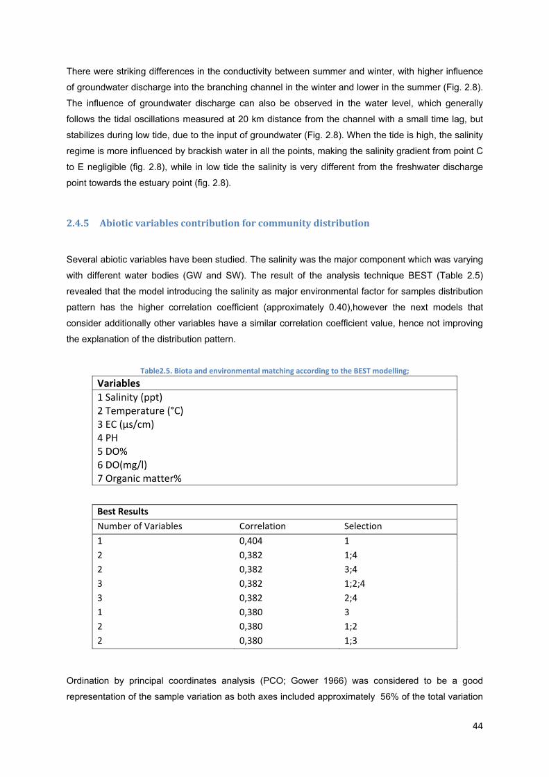
44  

There were striking differences in the conductivity between summer and winter, with higher influence

of groundwater discharge into the branching channel in the winter and lower in the summer (Fig. 2.8).

The influence of groundwater discharge can also be observed in the water level, which generally

follows the tidal oscillations measured at 20 km distance from the channel with a small time lag, but

stabilizes during low tide, due to the input of groundwater (Fig. 2.8). When the tide is high, the salinity

regime is more influenced by brackish water in all the points, making the salinity gradient from point C

to E negligible (fig. 2.8), while in low tide the salinity is very different from the freshwater discharge

point towards the estuary point (fig. 2.8).

 

2.4.5 Abioticvariablescontributionforcommunitydistribution 

Several abiotic variables have been studied. The salinity was the major component which was varying

with different water bodies (GW and SW). The result of the analysis technique BEST (Table 2.5)

revealed that the model introducing the salinity as major environmental factor for samples distribution

pattern has the higher correlation coefficient (approximately 0.40),however the next models that

consider additionally other variables have a similar correlation coefficient value, hence not improving

the explanation of the distribution pattern.

Table2.5. Biota and environmental matching according to the BEST modelling; 

Variables 

1 Salinity (ppt) 2 Temperature (°C) 3 EC (µs/cm) 4 PH 5 DO% 6 DO(mg/l) 7 Organic matter% 

Best Results     

Number of Variables  Correlation  Selection 

1  0,404  1 

2  0,382  1;4 

2  0,382  3;4 

3  0,382  1;2;4 

3  0,382  2;4 

1  0,380  3 

2  0,380  1;2 

2  0,380  1;3 

Ordination by principal coordinates analysis (PCO; Gower 1966) was considered to be a good

representation of the sample variation as both axes included approximately 56% of the total variation

 

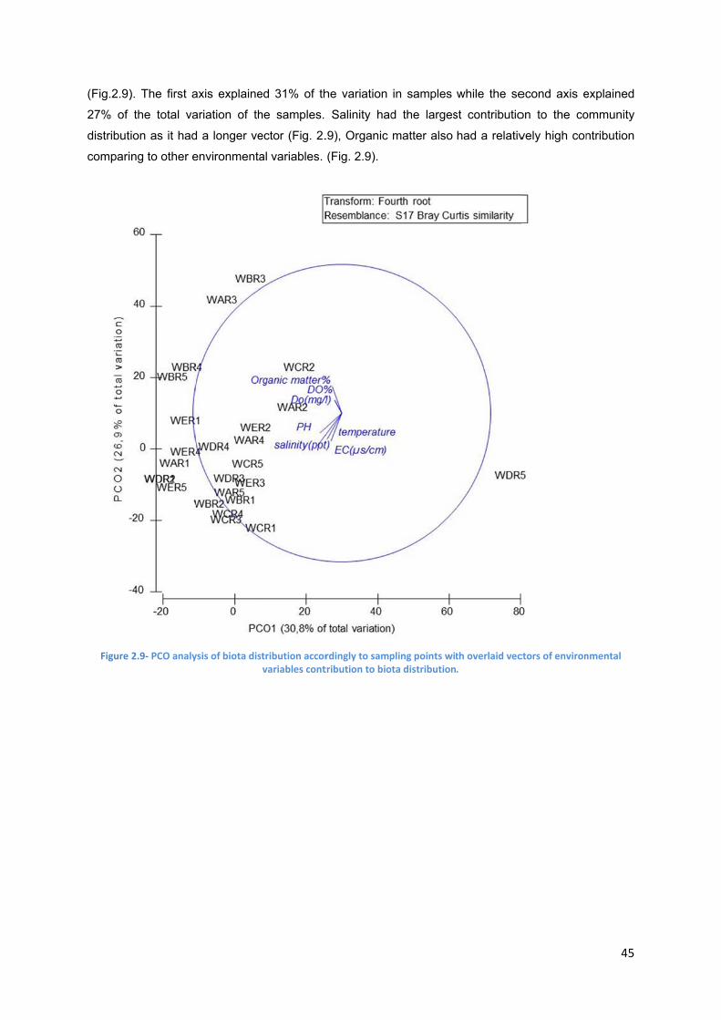
(Fig.2.9)

27% of

distribut

compari

Figure 

 

 

 

 

 

 

). The first a

the total va

ion as it had

ng to other e

2.9‐ PCO analy

axis explaine

ariation of th

d a longer ve

environmenta

ysis of biota dis

ed 31% of th

he samples.

ector (Fig. 2.

al variables.

stribution accorvariables cont

he variation

Salinity had

.9), Organic

(Fig. 2.9).

rdingly to samptribution to bio

in samples

d the larges

matter also

pling points witota distribution

while the se

st contributio

had a relativ

th overlaid vec. 

econd axis e

on to the co

vely high con

ctors of environ

45 

explained

ommunity

ntribution

nmental 

46  

2.5 Discussion

2.5.1 Groundwateravailabilityandcommunitypredictions

The present work represents the first study in Portugal examining the influence of groundwater

availability on estuarine biodiversity. There was a correspondence of the community distribution

pattern to a salinity gradient established by groundwater discharge into the estuary. There was also

indication that temporal differences in macrobenthic presence may occur between in dry and wet

season, although further evidence is required. Taken together these results indicate that the benthic

estuarine community can be potentially used as a surrogate for evaluating changes in the ecosystem

salinity. Climatic predictions indicate that groundwater will be used in higher human demands in South

Portugal due to increased drought periods (Santos et al., 2002), and that global groundwater

availability and quality will diminish (Danielopol et al., 2003). There is a predicted scenario for the

studied area of reduced aquifer recharge and increased sea level rise followed by a potential saline

intrusion, which can change the salinity condition of the Querença- Silves aquifer (Santos et al., 2002;

Monteiro et al., 2007). This condition can be aggravated by the risk of overexploitation for irrigation

and public water supply and thus, the biological community is likely to suffer specific shifts related to

salinity, which can be detected under a biologically orientated monitoring programme.

It is known from literature that there is also a close relationship between sediment grain size and the

trophic structure of benthic communities in estuaries and, in general, suspension feeders are more

common in coarser sandy sediments while deposit feeders seem to have a preference for muddy

sediments (Chainho, 2008). In the present study, sediment type is primarily a function of flow, since

the transport and deposition of sediment particles from estuary into the channel are regulated by the

diurnal tidal movement. At the upper part of the channel, in the location of the GW input (Point C),

there was more coarse sandy sediment, while the other points toward the estuary (point D and E) had

more fine muddy sediment type. Seasonal or even daily changes of the sediment structure due to

fluctuations in tidal movements can be regarded as physical disturbances and affect the colonization

by benthic invertebrate species. For the present study, the grain size was not measured due to

logistic constrains, therefore it is possible that part of the 50% of the unexplained variation within the

total variation found in our data can be due to sediment type.

The organic matter content in the sediment and salinity are known to be the two most important

physic-chemical features influencing benthic distribution in other Portuguese estuarine systems

(Nunes et al., 2008; Teixeira et al., 2008). Certain aquatic species such as Capitella capitata has

been documented be a reliable indicator of organic enrichment pollutant (Macleod et al., 2004). In the

present study Capitella capitata found to be more abundant in location B with higher Organic

matter%.

The community showed clear evidence of responding to the influence of groundwater discharge and

times. For instance, several species of the Polychaeta class were more abundant at the freshwater

discharge location and at the end of the wet season. Similar groundwater dependence has been

found for rotifers in Brazilian estuaries but in their case for the dry season (Medeiros et al., 2010). The

present study allows the prediction that a decrease in the abundance of the some Polychaeta species

47  

and increase in Isopoda, are potentially early warnings of a reduction in groundwater input into this

habitat interaction. The abundance of the Spionidae, Alkmaria romijni and Hediste diversicolor will

potentially diminish greatly under severe reduction of groundwater discharge into estuarine

ecosystems. This is potentially more visible at the end of the dry season when groundwater

availability is likely to be more limited .Conversely, the Isopod Cyathura carinata and Hediste

diversicolor, will potentially remain in the current abundance level unless other environmental

parameters such as organic matter or environmental variables (e.g. pH, temperature) shift. Some taxa

such as Oligochaeta, the second most abundant specimens of our samples, and Capitella Capitata

did not show any pattern with groundwater discharge as they were abundant both at the end of dry

season and freshwater discharge points. This macrofauna Polychaeta is described as a bacterial

pollution indicator and it corresponds to a brackish-saltwater species found in Mediterranean, Atlantic,

Arctic and pacific Oceans (Heyward and Ryland, 1995). Subclass Oligochaeta are known to tolerate a

wide range of salinity since some of their species are fresh water and some are brackish water

species (Chapman and Brinkhurst, 1980; Oikos, 1969). The present study sampled area is a

protected site where aquatic biodiversity is mainly influenced by natural shifts in the tidal cycle and

level of groundwater discharge directly from the aquifer. As discharges cause salinities as low as 0.5

ppt, the organisms adjacent and downstream to the point of groundwater input into the estuary are

directly exposed to sharp salinity shifts. This is analogous to the intertidal rocky shore habitat, as the

fauna therein is also subject to cyclic changes in the presence/absence of water coverage and salinity

levels. If the groundwater discharge is hindered and increased salinities occur, then the composition

and abundance of the faunal community characterised in the present study is likely to vary.

2.5.2 Variationingroundwaterdischargeandfood‐webimplications 

The Polychaeta Hediste diversicolor and Alkmaria romijni were found to be sensitive to groundwater

deficit as they are assossiated to freshwater resources. Results indicated that the abundance of

species Isopode Cyathura carinata and the Polychaeta Heteromastus filiformis varied significantly

with the salinity gradient created by the groundwater discharge into the estuarine habitat and they can

potentially be more sensitive to variations in groundwater input into the estuary. These taxa are

important food items for many commercially important estuarine fish, for example the European

flounder Platichthys flesus (Linnaeus, 1758) and Solea solea (Linnaeus, 1758) (Cabral, 2000;

Pasquaud et al., 2010). There are 36 commercially important fish species in the Arade estuary,

indicating the importance of this ecosystem as a nursery for many commercial species (Gonçalves et

al., 2004). Hence, under a predicted climatic scenario of reduction in the groundwater discharge rate

into the estuary, the macrobenthic species found here to be more associated with the groundwater

discharge point such as the Oligochaeta; will likely have their abundance reduced. This may have

bottom-up cascade effects into their predatory fish mentioned above, which will see their prey

availability reduced. Such cascading trophic links and effects should be evaluated and taken into

consideration in a monitoring programme, as shifts in the abundance of those fish species can be also

early warnings signals of changes in prey availability, albeit sampling of invertebrates is logistically

48  

easier. Global climate change effects are considered a major threat to estuarine fishes and their

fishery (Roessig et al., 2004), to the structure and dynamics of estuarine macrobenthic communities

(Grilo et al., 2011), and also to coastal fresh groundwater resources (Ranjan et al., 2006). Hence,

groundwater input into estuarine systems can be a key bottom-up factor regulating both food webs

and biodiversity levels. Benthic communities were shown here to provide an indirect method to

evaluate changes in salinity in the interface between aquatic habitats encompassing groundwater

systems. It is important that future monitoring programmes include an assessment of the spatial and

temporal variability of the species identified here as potential responders to groundwater availability.

.

 

49  

Chapter 3: Accessing stygofauna through wells: a window for evaluating GW condition?

 

 

 

 

 

 

 

 

 

 

 

 

 

 

 

 

 

 

50  

3.1 Abstract 

In coastal areas, groundwater is vulnerable to salinization by intruding natural seawater which makes

it unsuitable for drinking and agricultural use. In arid /semiarid areas such as in the present study

case, climate is expected to aggravate this problem, due to the combined effect of rising sea levels

and reduced recharge of aquifers associated with the expected decrease in precipitation and average

temperature increase. The purpose of this study was to examine the sensitivity of wells fauna to

variation in groundwater salinity/conductivity accessed through wells. Also, it aimed to provide ground

breaking biological data to integrate the use and conservation of groundwater dependent fauna into

aquifer management. Six wells were selected for sampling in which four of them were more

associated to salinization risk as they are located close to Arade estuary, whereas the other two wells

are relatively far from the sea. Wells fauna was sampled with the use of a phreatobiological net

developed for large diameter wells, as well as a well sediment sampling device developed for the

present study (WSSD). Except for the three groups including Oligochaeta, Gastropoda and

Coleoptera, all sampled species belonged to the Crustacea taxa (Daphnia, Cladocera, Cyclopoida,

Harpacticoida, Ostracoda, Amphipoda). A total of 612 specimens comprising so far 19 species were

identified for all 6 wells. Fauna identification was only completed for some families in Crustaceans

including Amphipods, Copepods, and Ostrocods, but further studies are on-going. The Order

Cyclopodia dominated in all 6 wells with relatively high diversity. There was an apparent relationship

between salinity level of well water and stygofauna presence. The results of multivariate analysis

indicate that wells with high salinities were separated from wells with low salinity records. The species

Eucyclops speratus (Lilljeborg, 1901), Eucyclops hadjebensis (Kiefer, 1926), Megacyclops viridis

(Jurine 1820) and Acanthocyclops sensitivus (Graeter & Chappuis, 1914) were particularly associated

with low salinity conditions (Electrical conductivity<1500 µs/s), hence being potential indicators for

saline intrusion if their abundances decrease greatly. Conversely, the taxa Halicyclops sp. is a

possible indicator of high salinity conditions (Electrical conductivity>6000 µs/s). The greatest diversity

and highest abundance were found in the lowest salinity condition (well Q4). The comparison

between the two sampling methods indicated that the Phreatobiological net is more effective in

gathering representative samples, particularly from Cyclopodia which are generally good swimmers,

while the WSSD net is more suitable to have sample groups adapted to benthic life such as

Harpacticoids and Ostracods. Further studies on high and low salinity wells are necessary to

disentangle the relation between species presence and salinity conditions.

 

51  

3.2 Introduction

Groundwater is one of the most essential basic resources for human life. In Europe, 65% of the

drinking water originates directly or indirectly from the subsurface (Steube et al., 2010). Climate

change will have a profound impact on all water resources including groundwater, however compared

to surface water resources, the underground water has not received as much as attention in climate

change risk issues (Bates et al., 2008). This may be because aquifers are considered more resilient

than surface water and, because the quality of surface water is seldom considered a serious threat to

groundwater quality, because it is considered to be filtrated and diluted as it enters the aquifer.

Conversely, surface waters are considered more vulnerable to quality degradation due to their easy

accessibility. The aquifer salinization is the most widespread phenomenon of groundwater

contamination (Kim et al., 2003) and may occur when groundwater levels are abnormally low. Climate

change aggravates this problem in arid and semi-arid regions due to predicted future scenario in

which the temperature and groundwater demand increase and precipitation decreases. Groundwater

resources are considered to be under increasing pressure due to large abstraction rates for various

water-consuming activities (e.g. agriculture activity such as irrigation), public water supply

(consumption) and industry (Stigter et al., 2009). Reductions in recharge can become very significant

due to acceleration in groundwater pumping in the following decades (Santos et al. 2002, Giorgi 2006:

Jackson et al., 2011). The combined effect of prolonged and large extractions from the aquifer and

reduced recharge in coastal areas can lead to seawater intrusion, a serious problem worldwide,

including the Mediterranean countries.

Groundwater ecology is a developing science in the last few decades, dealing with structural and

functional aspects of the organisms inhabiting the water subsurface and with the relationships

between these organisms and their surrounding aquatic environment (Danielopol et al., 2007). For

many years, groundwater was considered unlikely to be a habitat for diverse invertebrate

assemblages due to ‘extreme environment’ associated with absence of sunlight. However, recently

this hypothesis has been challenged and it is acknowledged that biological diversity of groundwater is

much greater than formerly appreciated and much more widespread (Humphreys, 2009; Danielopol et

al. 2001; Danielopol and Pospisil 2001). In 1986, Botosaneanu listed about 7000 groundwater species

worldwide (Ferreira et al., 2007). However, the number of subterranean taxa is likely to be severely

underestimated because of the lack of investigations in this area and the lack of taxonomic expertise

for several subterranean groups. In the groundwater ecosystem, different animal types occur and

there are several classification frameworks of groundwater invertebrates in the literature. A most

accepted classification considers their preferred habitat and resultant behavioural, physiological and

morphological features (Gibert, 2001). Three categories are distinguished in this classification

including (i) Stygoxenes- organisms that have no affinities with groundwater systems and but

occurring there accidentally, (ii) Stygophiles- encompass a number of species that actively exploit the

resources of the groundwater environment for part of their life cycle and, (iii) Stygobites- who are

specialised subterranean forms that complete their whole life cycle exclusively in subsurface water

52  

(Gibert, 2001). The risk of species extinction is expectedly high for Stygobites because they have a

narrow distribution range and are more in danger in face of the increase in multiple anthropogenic

pressures (Ferreira et al., 2007). The biogeographical distribution of groundwater fauna is different

around Europe and in southern Europe, where the climate stayed moderate during the various

glaciation periods; most of the old Tertiary fauna still persists. These regions are characterised by a

diverse, endemic, exclusively subterranean dwelling fauna (Pipan and Culver, 2007). In Europe, karst

groundwater systems contain a pervasive and significant fauna that compares with some of the

richest sites known anywhere in the world (Boulton et al., 2003; Danielopol et al., 2007). According to

Galassi (2009), crustaceans represent about 10% of the total number of invertebrate species known

from fresh water world-wide, of which Copepoda have 2814 described species, Ostracoda about 1936

species and Amphipods 1870 species, being by far the most species-rich crustacean groups (Dole-

Olivier et al., 2000; Galassi et al., 2009; Stoch and Galassi, 2010). The stygofauna in temperate

regions is dominated by crustaceans (65% of species) and molluscs (22%). Temporal trends in the

cumulative number of groundwater and surface water species suggested that groundwater comprised

more crustaceans than surface freshwater (Ferreira et al., 2007).

The qualitative and quantitative status of groundwater is assessed based on the chemical and

hydrogeological parameters  (Steube et al., 2009). However, knowledge on the drivers for the often

patchy distribution of groundwater fauna is poor, which limits predictive conclusions. Besides that,

there is a lack of sufficient information on the taxonomy, autecology and physiology (e.g. sensitivity to

pollutants) with respect to groundwater organisms. Nevertheless, several authors have already

stressed the use of groundwater invertebrates for biomonitoring purposes and the assessment of the

ecological status (Steube et al., 2009; Bright et al., 1998; Claret et al. 1999). Although physical–

chemical monitoring and routine analyses cover most of the contaminants relevant for human health,

there are number of arguments which support the complementary use of bioindicators to assess

subterranean resources including i) Detection of effects by short-term (pulses of) contaminant impacts

because it is possible to collect organisms in short-term, mid-term and long-term impacts over time

can reflect an ‘integrative’ picture of water quality and ecosystem status, ii) Indirect detection of ‘new’

pollutants at low but ‘chronic’ concentrations which are not yet detectable by other methods (Steube

et al., 2009), iii) Evaluation of the hydrological connection between the surface and the aquifer. In

fact, groundwater fauna reflect structural conditions of their habitat such as hydraulic conductivity,

heterogeneity of habitats in an aquifer and provide information on surface/subsurface hydrological

exchanges (Danielopol et al., 2007). Recently, environmental policy has started to consider

groundwater not only as a resource for high quality water but as a living ecosystem. In particular, the

Swiss Water Protection Ordinance (GSchV, 1998) and the EU Groundwater Directive (EU-GWD,

2006) mention ecological objectives to keep the biocoenosis in a natural state and to foster research

in groundwater ecology, respectively (Steube et al., 2010). In 2002, the European Commission

launched the PASCALIS programme (Protocols for the Assessment and Conservation of Aquatic Life

in the Subsurface), aiming to improve the evaluation of GW biodiversity and to develop guidelines and

strategies for its conservation in six European regions (Gibert, 2001). Assessing the biodiversity and

abundance response of groundwater fauna sampled in aquifers of differing groundwater

53  

characteristics allows evaluating impacts such as seawater intrusion on the vulnerable groundwater

ecosystem. Knowledge on groundwater biodiversity is currently biased towards penetrable karstic

habitats (caves), whereas other common habitats such as those found in porous aquifers have been

neglected! Planning an efficient sampling strategy is strongly constrained by difficulties in accessing

the subterranean realm, especially in deep phreatic habitats. As a consequence, sometimes it may

not be possible to distribute samples sites where it would be necessary, but only where access is

possible through a limited number of outputs (springs, resurgences) or few “windows” (caves,

wells)(Gibert, 2001). Within an existing fragmented frame of knowledge of subterranean biodiversity,

the present contribution aimed to (i) study the community structure of stygofauna sampled in wells

and, (ii) its relation to groundwater condition, i.e. salinity at the Central Algarve. Reliable assessments

of groundwater biodiversity are urgently needed to resolve current issues relating to the protection of

aquifers.

 

3.3

3.3.1

The stu

prelimina

the stud

groundw

(establis

selected

occurred

and one

Fig.3.1 a

3.3.2  

Tempera

portable

measure

the cond

probes

measure

Methods

Studyare 

udy area is lo

ary well inve

dy aims wer

water saliniti

shed with d

d: high-salini

d in Decemb

e spring was

and wells 2,

Figure 3.1‐ 

Fieldabio

ature (°C), d

e meters at

ed with fixed

ductivity mea

installed an

ements.

s

ea:

ocated in the

entory was m

re selected.

es so as to

ata loggers)

ty wells-EC

er 2010. At l

selected for

3, 22, 23, 25

Location of the

oticmeas

dissolved ox

each samp

probes in a

asurements

d their valu

e discharge a

made in study

The curren

o detect res

) of several

> 6000 μS/

east two we

r sediment sa

5 and 26 wer

e inventoried w

surements

xygen (mg.l-

pling occasi

long term su

value for ev

ue in the ta

area of the Q

y zone and w

t stygofauna

sponses to

l wells was

/cm, and low

lls per salinit

ampling. The

re sampled.

wells. Wells num

s

1 O2) and p

ion (Table

urvey for wel

very 6 minut

able is the a

Querença-Sil

wells with the

a status was

this parame

considered

w-salinity we

ty category w

e location of

mber 2,3, 22,23

pH were me

3.1). Elect

lls number 1

tes. Wells nu

average valu

ves aquifer.

e most suitab

s evaluated

eter. The a

and two w

ells -EC< 14

were sampled

the inventor

3,25 and 26 we

easured dire

trical condu

, 2 4 and 5. T

umber 3 and

ue of sever

In an initial

ble characte

in wells of

average yea

well categor

400 μS/cm. S

d, in a total o

ried wells is

ere sampled. 

ectly in the f

ctivity (µm/c

The probes

d 6 did not

ral in situ re

54 

phase, a

ristics for

differing

r salinity

ies were

Sampling

of 6 wells

shown in

field with

cm) was

recorded

have the

egistered

 

 

Table3.

W 

S

 

3.3.3 Two sam

phreatob

(WSSD)

deep or

is descri

75

Mecha

.1‐. Wells abiot

ell code 

Q5 

Q1 

Q3 

Q6 

Q4 

Q2 

Spring 

Sampling

mpling device

biological ne

) developed

have shallow

ibed in Fig.3

5 cm

40µm

talic ains

tic and morpho

“figure 1” by co

PH  

7.75 

7.44 

7.49 

7.58 

7.03 

7.37 

7.25 

gdesign:

es were used

et for sampl

by the CVR

w water. The

.2 (Cvetkov

Figur

ologic character

odes 2, 3, 22, 2

Depth (m) 

    2 

    3 

        3.65 

      >30 

     >10 

           4 

        n.a. 

d to assess g

ing in large

M team for d

e phreatobiol

1968, Gibert

Me

fr

20µm

Plasti

re 3.2‐  Phreato

ristics. Wells n

23, 25 and 26 re

EC (µm/cm)

12987 

   8162 

6100 

    848 

 1390 

 9113 

759 

groundwater

diameter w

directly colle

logical net w

t, 2001).

etalic circular 

rame 40cm

ic valve

obiological net 

umbers 1, 2,3,4

espectively. n.a

Dis.  Oxi.(mg/l)

 1.5 

 4.4 

 0.88 

 6.15 

 3.61 

 3.72 

 6.38 

r fauna asso

wells and a W

ecting sedim

which can onl

and its deploy

4,5 and 6 refers

a.‐not available

 Temp(C) 

    15.3 

19.63

15.71

15.43

17.6 

16.2 

      20 

ciated with th

Well Sedime

ent in the we

y be used in

ment. 

s to wells illust

e. 

p  Hyd.h(m

     1.7 

3        1.3 

1         3 

3         n.a

       5.6 

       0.9

      n.a.

he well sedim

ent Sampling

ells that are

n large diame

55 

trated in 

ead ) 

. 

5 

_ 

ment: the

g Device

not very

eter wells

 

 

This net

(PASCA

circular f

to rubbe

exit. Th

moveme

encomp

column.

the well

PASCAL

sampling

develope

directly c

of benth

of the W

Decemb

The Phr

to collec

this dev

After ea

material

was add

were tak

t is an ackno

ALIS project)

frame of 40 c

er) which allo

he net creat

ents of the n

asses weigh

According t

l at least 10

LIS and sev

g stygofaun

ed another

collected. Th

hic animals. T

WSSD net is

ber 2010.

reatobiologic

ct sediment f

ice. Three re

ch replicate

stored into

ded to the co

ken for which

owledged sam

). As it is ill

cm diameter

ows the swim

tes an asce

net, subsequ

hts that distu

to the PASC

0 times thro

veral other w

a is verified

net- sample

his device wa

The use of tw

s illustrated i

al net was u

from the disc

eplicated net

collection, th

sealed conta

ontainer to p

h fauna ident

Figure3.3

mpling metho

ustrated in F

r. At the base

mming fauna

ending curre

uently captu

urb the sedi

CALIS projec

ough the ent

works (Giber

d for large d

r (WSSD) fo

as designed

wo different

n Fig 3.3. S

sed to collec

charge point

t deploymen

he net collect

ainers and fix

osteriorly sim

tification and

‐ Well Sedimen

od, with exis

Fig.3.2 the 4

e of the mes

a and the ben

ent in the w

uring the sus

iment and b

ct recommen

tire water co

rt, 2001) th

diameter we

or shallow w

so as to min

methods allo

Samplings co

ct samples in

of a spring a

ts and at lea

ting glass wa

xed with 97%

mplify the so

d quantificatio

nt Sampling De

ting samplin

40µm mesh

h cone there

nthic fauna t

well by suc

spended ani

bring the ani

dation (Gibe

olumn. With

he efficiency

ells. Howev

wells in whic

nimise the dis

owed an effic

ollections fro

n 6 wells, wh

and from 1 w

ast one WSS

as washed in

% ethanol al

orting of colo

on was made

evice and its de

g protocols a

cone is mo

e is a valve (a

o be collecte

cessive upw

mals. The lo

mals of sed

ert, 2001) the

in the frame

of the phre

ver, in the p

h the bottom

sturbance, an

ciency comp

m the wells

hile the WSS

well where its

SD replicate

nto the 50µm

cohol. The ro

ured fauna.

e.

ployment. 

at the Europ

ounted on a

aluminium co

ed and preve

ward and d

ower end of

diment into t

e net must d

ework of the

eatobiologica

present wor

m sediment

nd potential

parison. The

were carrie

SD net was o

s depth allow

were taken

m mesh sieve

rose Bengal

In total, 20

56 

ean level

a metallic

onnected

ents their

ownward

f the net

he water

draw into

e project

al net for

rk it was

could be

damage,

structure

ed out on

only used

wed using

per well.

e and the

chemical

samples

 

57  

3.3.4 Wellsfaunaassessment

The Crustacean was selected as the target group because they are the dominant groups of the

stygofauna in temperate regions (65% of species). The presented study considered only the factor

salinity subdivided in high salinity and low salinity wells. This design does not allow withdrawing

conclusions on temporal patterns as no replicated were measured within along the time period. Three

replicates were taken at each location and time combination. Multifactorial analyses were made in the

PRIMER+ package (Clarke and Warwick, 2007; Anderson et al., 2008). The similarity percentage

breakdown procedure (SIMPER) (Clarke & Warwick, 1994) was used to determine the contribution of

individual taxa to the dissimilarity between and within the factors, and also to identify the species most

contributing for significant factorial differences. MDS and dbRDA ordination techniques were

calculated to graphically examine the samples distribution pattern. For all tests, the Bray-Curtis

similarity measure, the fourth-root transformation and 9999 permutations were used for all biotic data,

while for abiotic data was normalized and the Euclidean distance measure used in the PRIMER+

calculations. The fourth root transformation was applied to give more weight to the rare species and

reduced the weight of the dominant species. Obligate stygofauna species were separated from the

stygoxene and stygophile species. The wells with easy accessibility to bottom sediment due to its

shallow depth were selected to be sample of the two different devices (Phreato net and WSSD net)

allowing a comparison of fauna structure and composition.

3.4 PreliminaryResultsandinterpretation

3.4.1 Faunageneralcharacterization

A total of 612 crustacean organisms were sampled in total. A total number of 19 species was

identified and corresponds to brackish water organisms, Stygobites, Stygoxenes and Stygophiles of

the identified fauna corresponds to Amphipods, Copepods and Ostracod (Table 3.2.). The Order

Cyclopodia from the class Copepod was the most dominant taxa. With 53 families, the order

Cyclopodia revealed to be the most diverse taxa with 11 identified species in the present study. The

taxa richness for the wells was highest at the well number 4 with also had the lowest salinity recorded.

Faunal assemblages were dominated by Stygobites species and Stygophiles and/or Stygoxenes

never contained more than 32% of the total number of invertebrates.

The order Harpacticoida is well adapted to benthic life because they are typical crawlers, walkers, and

burrowers (Galassi et al., 2009). They can be found in freshwater and in saline water ecosystems

depending on the species. Here, Harpacticoida were found in the spring sampling location and in the

well Q1. The spring was sampled with the WSSD net, considered more likely to collect this type of

benthic animal. Well Q1 and 2 had always high salinity (> 7000 µs/cm) comparing to the other

sampling wells, potentially because they are closer to the Arade estuary.The Halicyclops sp. is a

cosmopolitan Cyclopodia genus of the family Cyclopidae, widely distributed in several kinds of surface

brackish water bodies (Chang, 2012).

58  

Table 3.2‐ Identified species of Cyclopodia, Ostracod, Amphipod and Copepod sampled from wells. Shaded cells represent absence and unshaded cells represent a taxa absence. 

Q1  Q2  Q3  Q4  Q5  Q6  Spring 

Cyclopodia  

33 0 34 48 209 42 6

Halicyclops sp.  

Eucyclops graeteri (Chappuis 1927) 

Eucyclops serrulatus  (Fischer, 1851) 

Eucyclops hadjebensis  

Eucyclops speratus  

Megacyclops brachypus (Kiefer, 1954) 

Acanthocyclops sp.  

Acanthocyclops sensitivus  

Megacyclops viridis  

Macrocyclops sp.  

Macrocyclops albidus (Jurine, 1820) 

Ostracoda  

2 0 31 171 6 1 1

Cypria ophtalmica  (Jurnine 1820) 

Cypridopsis vidua (O. F. Müller, 1776) 

Bradleycypris oblique (Brady, 1868) 

Amphipoda  1 12 1 1 0 3

Gammaridae  

Sphroma sp.  

Gammarus sp.  

Gammarus pulex (Linnaeus,1758)  

Copepoda  2 2 3

Harpacticoida  

 

Its occur

The gen

Eucyclop

number

of individ

influence

Eucyclop

found in

being a

moderat

Acantho

and Woj

setae an

6 wells

(stygoxe

Howeve

Cypridop

family G

pulex is

(oxygen

1990). In

rrence in we

nus Eucyclo

ps graeteri i

Q5 and Q6)

duals. Well n

e by fresh/gr

ps speratus

n the spring

a potential i

tely eutroph

ocyclops sen

jtasik, 2009)

nd antennal

. The most

ene, stygoph

er, they were

psis vidua) a

Gammaridae.

a freshwate

and ammon

n Fig. 3.4 so

ell Q1 highlig

ops was the

s a hypogea

). This was th

number Q4 h

roundwater.

were found

location. Th

indicator of

ic water, bu

nsitivus found

). Ostracods

swimming b

t dominant

hile). They w

e more num

are also epig

They have

r species tha

nia), inorgan

me pictures

hts the fact t

dominant s

an (Stygobite

he most abu

had the lowe

The two Sty

d in the men

is species w

the presen

ut it can als

d only in wel

are swimm

ristles for pro

Ostracod s

were found in

merous in we

gean (stygox

wide distribu

at is sensitive

nic ions (pH)

representing

that this hab

specimens o

es) found in

ndant specie

st salinity re

ygobite Eucy

ntioned well.

was also fou

nce of grou

so occur in

ll Q4, is a co

ers or crawl

opulsion. Th

species was

n wells with

ell Q4. The

xene, stygop

ution and can

e to several

) and organic

g stygofauna

itat is influen

of the subfa

wells with d

es which con

cord indicatin

yclops hadjeb

. The Eucyc

nd in the low

undwater. M

groundwate

ommon grou

lers. Swimm

ree species

s Cypria op

different ch

other two s

hile). All Am

n survive wid

water polluti

c compound

can be obse

nced by estu

mily Eucyclo

different salin

ntributed 37%

ng that this w

bensis (semi

clops speratu

w salinity we

Megacyclops

er as a styg

ndwater spe

ing species

of ostracod w

phtalmica, a

haracteristics

species (Cyp

phipod taxa

de range of s

on including

ds (dichloroa

erved.

arine brackis

opinae. The

nity categori

% of the tota

well is under

ibenthic spec

us species w

ells (Well Q4

viridis can

goxen (Reid

ecies (Miodu

use their an

were identifi

an epigean

s in terms of

pridopsis vid

corresponde

salinities. Ga

g metals (zinc

aniline) (Malt

 

59 

sh water.

species

es (wells

l number

r a strong

cies) and

was also

4), hence

tolerate

d, 2001).

chowska

ntennular

ed for all

species

f salinity.

dua and

ed to the

ammarus

c), gases

by et al.,

 

Figure3serrulatus

 

3.4.2  

The spe

Table3

So

SaLoRTo

The MD

categori

separate

the rem

species)

Figure 3

3.4‐some repres  / Cypridopsis

Speciesd

ecies distribut

3.3‐ Permanova

ource 

a o x Sa es otal 

DS ordination

es (Fig 3.5)

ed in the ord

aining low s

).

3.5‐MDS ordinaeach well 

esentive Stygofas vidua/ Harpac

distributio

tion was sign

a analysis of thenumber of 

n showed tha

) Wells num

dination plot.

salinities poin

ation of  wells f(R1‐R3)groupe

auna, sequentlcticoida/ Macr

on

nificantly exp

e wells fauna fopermutations u

df   S

1  2

4  2

12  3

17   6

at the commu

mber 4 (Q4)

However o

nt. This is m

fauna samples ed into two gro

ly from left up rocyclops albidu

plained the s

or factors salinused was 9999

SS 

2198  2

28243  7

30577  2

61016 

unity structu

and 6 (Q6

ne replicate

mostly due to

collected fromups of salinity 

to right down: us/ Eucyclops /

alinity gradie

nity (high and lo9 (Sa= salinity,L

MS  Pse

2196  0,3

7060  2,7

2548 

    

re varied be

), which are

(replicate 3)

o the low nu

 6 different wecategories (H: 

Gamarus pulex/ Megacyclops 

ent (Table 3.

ow) and differeo‐ location). 

eudo‐F   P. (per

31102  1 

771  0,00

            

tween wells

e wells with

) from well Q

umber of tax

ells (Q1‐Q6), wihigh and L:low

ex/Eucyclops seviridis/ Gamm

.3).

ent wells locati

rm) U. perms

15 

001  9903 

         

with differen

low saliniti

Q6 is separa

xa in this rep

ith three replicw salinities).

60 

errulatus arus pulex 

on. The 

s 

nt salinity

es, were

ated from

plicate (1

ate from 

61  

The SIMPER analysis reflected that there was a relatively high average dissimilarities (81,66)

between two group of wells based on their salinity properties. Within the context of this test, the

species that contributed the most for significant differences between two groups of wells are identified

in Table 3.4.

Table 3.4‐ SIMPER analysis identifying the species that contributed the most for differences between wells with high and low salinities 

  G.High  G.Low         

  Av.Abund  Av.Abud  Av.Diss  Diss/SD  Contrib%  Cum.% 

Cyclopodia  3.26  2.81  20.02  1.35  24.52  24.52 

Cypria 

ophtalmica 

0.70  3.12  18.11  0.73  22.18  46.70 

Eucyclops 

graeteri 

2.31  0.17  11.07  0.79  13.56  60.26 

Total Amphipod  0.64  0.57  7.04  0.66  8.62  68.88 

Macrocyclops sp.  0.00  1.07  4.91  0.43  6.01  74.89 

The taxa which contributed the most for dissimilarities between wells group were the total number of

Cyclopodia (25%) which, together with the species Cypria ophtalmica and Eucyclops graeteri 

represented 50% of the dissimilarities. Cyclopodia were more numerous in the high salinities wells

which can be due to having more sampled wells with high salinities. However, the epigean Ostracod

Cypria ophtalmica was more abundant in low salinities wells. The obligate groundwater species

Eucyclops graeteri  had higher abundance in the high salinities wells and, may have the same

justification as species Cypria ophtalmica. But here this species is very abundant in well Q5 which has

been characterised as high salinity well. The times series of electrical conductivity recorded periods

with very high salinities over 40000 µs/cm (months October and November) and relatively very low

salinity less than 2000 µs/cm (mostly in summer periods).The wide range of salinity variation in the

well may explain the presence of this true groundwater species in periods that have low salinity

measurements.

3.4.3 Samplingdevicecomparison

Well Q5 was sampled using the Phreato net and WSSD net methods. Three replicates were collected

with each device. Care was taken to use 1st the almost not disturbing WSSD so as to have

representative sub sequential nets samples. Also, the well was very wide, allowing sampling different

well areas with the two methods. The Total number of individuals, number of taxa, diversity and

richness captured with both devices were compared. The total number of individual was higher in

samples collected by the Phreato net; however the number of taxa was higher in samples collected by

WSSD device. Cyclopodia were more diverse in samples taken with the Phreato net while Ostracod

and Harpacticoida were more diverse in WSSD samples. This can be justified by the fact that

Harpacticoids and ostracods are well adapted to benthic life while Cyclopoids are generally good

swimmers (Dole-Oliver et al., 2000).

62  

        Table3.5‐ Taxa abundance sampled by Phreatobiological net and WSSD. 

Replicates  R1  R2 R3 

Phreato net       

Eucyclops graeteri  103  86  17 

Megacyclops brachypus    2   

Acanthocyclops sp.      1 

Bradleycypris obliqua  6     

WSSD net       

Eucyclops graeteri  2     

Acanthocyclops sp.    1   

Harpacticoida    2   

Cypria ophtalmica      2 

Cypridopsis vidua      1 

 

 

 

 

 

 

 

 

 

 

 

 

 

 

 

 

63  

Chapter 4: Main conclusion and future works

64  

4.1 MainConclusionsandfutureworks 

This study initiates baseline data on stygofauna and benthic invertebrate, interfacing different saline

condition. Biological indicators can be a functional tool to predict climate change effects if we

understand the factors influencing the habitat communities.

Within the first experiment evidence for estuarine fauna to be considered as a potentially valuable

indicator of variation in the input of groundwater into marine-freshwater interface habitats were

provided. The shifts in precipitation and temperature regimes predicted by climate change will lead to

enhancement in the demand on groundwater, altering the hydrologic balance on the marine-

groundwater interface such as in estuaries. Substantial aquifer exploitation threatens the wetlands

that constitute groundwater dependent ecosystems. The habitat alteration may affect the communities

from primary producers such as macrophytes communities until the higher trophic level such as fish

communities .Hence, benthic community identification and protection before any anthropogenic

disturbance are highly recommended (Seilheimer et al., 2009). Regarding the presence of

macroinvertebrates in the sediment of the Arade estuary in the Central Algarve, diversity was

relatively high with a total of 38 taxa being identified. Results indicate that there was a qualitative and

quantitative response of macroinvertebrate community to the salinity gradient inherent to the sampling

locations in the channel: those which tolerate low salinity were the most abundant at the location of

groundwater input, locations A, B, C. There were clear differences in Electrical Conductivity

(considered a surrogate for salinity) between summer and winter, with higher influence of

groundwater discharge into the channel during winter. The macroinvertebrate community structure

responded to this seasonal hydrological variation. Groundwater input into estuarine systems can

therefore be a key bottom-up factor regulating both food webs and biodiversity levels. If the

groundwater outflow is reduced, as predicted by aquifer modelling under climate change, then the

composition and abundance of the faunal community is likely to vary. As these organisms adapt over

time to disturbance and display different biological sensitivities between species, they give an indirect

method to evaluate changes of environmental features and generalised impairments. It is crucial that

future monitoring programmes include an assessment of the spatial and temporal variability of the

species identified here as potential responders to groundwater influence, because it allows assessing

interferences from external factors such as pollution originated from the main estuarine channel or

shifts in groundwater availability into the estuary.

The results from the second experiment were indicated that stygofauna can be potential indicators to

predict changes in the biodiversity in situations where a reduction or deterioration in groundwater can

significantly impact biodiversity. Recent climate change and groundwater exploitation have a strong

impact on groundwater quality. Saline intrusion into the groundwater resources is one of the

consequences. This situation has a great impact on local social and economic systems and the loss

of regional biodiversity and aquatic refuges (Mischkea et al., 2012). The results of the present study

allowed for understanding the general stygofauna inhabiting in the wells receiving recharge water

from Querença-Silves aquifer. There has been a resistance in using biological indicators to assess

65  

the groundwater conditions. This resistance reflects concerns about sampling costs, taxonomic

constraints, the lack of baseline data for comparison, and uncertainty about how to interpret

stygofauna data (Boulton, 2009).This work initiate the study on stygofauna in south of Portugal in the

hope of overcoming these restrictions and, providing baseline data for conservation planning for

future years. Within this experiment from well number 6, with low salinity condition some new species

were collected. They are small amphipods without eyes and have been identified to genus taxonomic

level and their identification into species level has not been completed since they are suspected to be

new to the science. In the climate scenario of decreased groundwater net recharge and intrusion of

brackish estuaries water into the aquifer, a shift in both identity and abundance of Stygofauna can

now be expected. This is in agreement with Boulton (2009) who indicate that there is a marked

difference among species in their response to water level changing (preliminary laboratory test).

Moreover, the ecological attributes of stygofauna makes them vulnerable to changes in habitat, which,

combined with their taxonomic affinities, makes them a significant issue to biodiversity conservation

(Humphreys, 2006).

In the same way, with this study we can start to understand some of the environmental factors such

as salinity and aquifer structure that correlate with groundwater fauna, particularly for the species

Eucyclops speratus, Eucyclops hadjebensis, Megacyclops viridis and Acanthocyclops sensitivus,

which were particularly associated with low salinity conditions, hence being potential indicators for

saline intrusion if their abundances decrease greatly.

The identification of this specialized fauna was made in collaboration with Dr. Sanda Iepure at the

Instituto Madrileño de Estudios Avanzados in Madrid, and its currently ongoing for the rest of the taxa,

taking longer than expected due to the detection of possible new species and due to the required

expertise to reach the ambitioned species level.

66  

Bibliography Ajami, H., Hogan, J., Maddock, T., Meixner, T., Troch, P., 2008. Quantifying spatial and temporal variability of mountain system recharge in semi-arid catchments, in:AGU Fall Meeting Abstracts, p. 1011. Alden, R., Weisberg, S., Ranasinghe, J., Dauer, D., et al., 1997. Optimizing temporal sampling strategies for benthic environmental monitoring programs. Marine Pollution Bulletin 34, 913–922. Ambrogi, A.O., Forni, G., 2004. Biotic indices. Biologia Marina Mediterranea 11 (Suppl. 1), 545-572. Anderson, M.J., Gorley, R.N., Clarke, K.R., 2008. PERMANOVAþ for PRIMER: Guide to Software and Statistical Methods. PRIMER-E Ltd, Plymouth. Attrill, M., Power, M., 2000. Effects on invertebrate populations of drought-induced changes in estuarine water quality. Marine Ecology Progress Series 203, 133–143. Bates, B., Kundzewicz, Z., Wu, S., Palutikof, J., et al., 2008. Climate change and water. Intergovernmental Panel on Climate Change (IPCC). Barros, M., Mendo, M., Negrao, F., 1995. Surface water quality in portugal during a drought period. Science of the total environment 171, 69–76. Bear, J., 1979. Hydraulics of ground water. Borja, A., Franco, J., P´erez, V., 2000. A marine biotic index to establish the ecological quality of soft-bottom benthos within european estuarine and coastal environments. Marine Pollution Bulletin 40, 1100–1114. Borja, A., Miles, A., Occhipinti-Ambrogi, A., Berg, T., 2009. Current status of macroinvertebrate methods used for assessing the quality of european marine waters:implementing the water framework directive. Hydrobiologia 633, 181–196. Bork, J., Berkhoff, S., Bork, S., Hahn, H., 2009. Using subsurface metazoan fauna to indicate groundwater–surface water interactions in the nakdong river floodplain, south korea. Hydrogeology Journal 17, 61–75. Boulton, A., Scarsbrook, M., Quinn, J., Burrell, G., 1997. Land-use effects on the hyporheic ecology of five small streams near hamilton, new zealand. New Zealand journal of marine and freshwater research 31, 609–622. Boulton, A., Findlay, S., Marmonier, P., Stanley, E., Valett, H., 1998. The functional significance of the hyporheic zone in streams and rivers. Annual Review of Ecology and Systematics , 59–81. Boulton, A., Humphreys, W., Eberhard, S., 2003. Imperilled subsurface waters in australia: biodiversity, threatening processes and conservation. Aquatic Ecosystem Health & Management 6, 41–54. Boulton, A., 2009. Recent progress in the conservation of groundwaters and their dependent ecosystems. Aquatic Conservation: Marine and Freshwater Ecosystems 19, 731–735. Bright, J., Bidwell, V., Robb, C., Ward, J., 1998. Environmental performance indicators for groundwater. Report No 4306/1, May 1998.Chang, C., 2012. Discovery of halicyclops continentalis (cyclopidae, halicyclopinae) from estuaries and salt marshes on the west coast of south korea. Animal Systematics, Evolution and Diversity 28, 12–19. Cabral, H., 2000. Comparative feeding ecology of sympatric solea solea and s.senegalensis, within the nursery areas of the tagus estuary, portugal. Journal of Fish Biology 57, 1550–1562. Claret, C., Marmonier, P., Dole-Olivier, M., Castella, E., 1999. Effects of management works on the interstitial fauna of floodplain aquatic systems (river rhone, france). Biodiversity and Conservation 8, 1179–1204. Castaneda, E., Drake, P., et al., 2008. Spatiotemporal distribution of lekanesphaera species in relation to estuarine gradients within a temperate european estuary (swspain) with regulated freshwater inflow. ecological indicators 34, 125–141. Chainho, P., Costa, J.L., Chaves, M.L., Lane, M.F., Dauer, D.M., Costa, M.J., 2006. Seasonal and spatial patterns of distribution of subtidal benthic invertebrate communities in the Mondego River, Portugal - a poikilohaline estuary. Hydrobiologia, 555.59-74.

67  

Chainho, M., 2008. Contribution to the development of biotic integrity assessment tools for Portuguese estuaries based on benthic communities. Ph.D. thesis. Universityof Lisbon, Portugal. Chang, C., 2012. Discovery of halicyclops continentalis (cyclopidae, halicyclopinae) from estuaries and salt marshes on the west coast of south korea. Animal Systematics, Evolution and Diversity 28, 12–19. Chapman, V., 1960. Salt marshes and salt deserts of the world. London: Leonard Hill (Books) Ltd. (Interscience Publ., Inc., New York). Chapman, P., Brinkhurst, R., 1980. Salinity tolerance in some selected aquatic oligochaetes. Internationale Revue der gesamten Hydrobiologie und Hydrographie 65, 499–505. Clarke, K.R., Warwick, R.M., 2007. In: Plymouth Marine Laboratory (Ed.), PRIMER-E, Version 6 (U.K.). Coulson, D., Joyce, L., 2006. Indexing variability: A case study with climate change impacts on ecosystems. Ecological Indicators 6, 749–769. Cvetkov, L., 1968. Un filet phr´eatobiologique. Bull. Inst. Zool. Mus. Acad. Bulgare. Sci., Sofia 27, 215–218. Dale, V., Beyeler, S., 2001. Challenges in the development and use of ecological indicators. Ecological indicators 1, 3–10. Danielopol, D., Pospisil, P., Rouch, R., 2000. Biodiversity in groundwater: a large scale view. Trends in ecology & evolution 15, 223. Danielopol, D., Pospisil, P., 2001. Hidden biodiversity in the groundwater of the danube flood plain national park (austria). Biodiversity and Conservation 10, 1711–1721. Danielopol, D., Griebler, C., Gunatilaka, A., Notenboom, A., et al., 2003. Present state and future prospects for groundwater ecosystems. Environmental Conservation 30, 104–130. Danielopol, D., Griebler, C., Gunatilaka, A., Hahn, H., Gibert, J., Mermillod- Blondin, G., Messana, G., Notenboom, J., Sket, B., 2007. Incorporation of groundwater ecology in environmental policy. Groundwater Science and Policy, London The Royal Society of Chemistry, RSC Publishing . Dauer, D.M. 1993. Biological criteria, environmental health and estuarine macrobenthic community structure. Marine Pollution Bulletin 26, 249–257. De Pauw, N., Ghetti, P., Manzini, P., Spaggiari, D., 1992. Biological assessment methods for running water. River water quality, Ecological assessment and control , 217–248. Díeza, I., Bustamante, M., Santolaria, A., Tajadura, J., Muguerza, N., Borja, A., Muxika, I., Saiz-Salinas, J., Gorostiaga, J., 2012. Development of a tool for assessing the ecological quality status of intertidal coastal rocky assemblages, within atlantic iberian coasts. Ecological Indicators . Dole-Olivier, M., Galassi, D., Marmonier, P., Creuz´e des Chˆatelliers, M., 2000. The biology and ecology of lotic microcrustaceans. Freshwater Biology 44, 63–91. Eamus, D., Froend, R., 2006. Groundwater-dependent ecosystems: the where, what and why of gdes. Australian Journal of Botany 54, 91–96. Elliott, M., Quintino, V., 2007. The estuarine quality paradox, environmental homeostasis and the difficulty of detecting anthropogenic stress in naturally stressed areas. Marine Pollution Bulletin 54, 640–645. Erwin, K., 2009. Wetlands and global climate change: the role of wetland restoration in a changing world. Wetlands Ecology and Management 17, 71–84. EUCYCLOPINAE, K., EUCYCLOPS, C., Cyclopoida. available at http://www.luciopesce.net/copepods/eucyc2.htm. Euliss, N., LaBaugh, J., Fredrickson, L., Mushet, D., Laubhan, M., Swanson, G., Winter, T., Rosenberry, D., Nelson, R., 2004. The wetland continuum: a conceptual framework for interpreting biological studies. Wetlands 24, 448–458. Ferreira, D., Malard, F., Dole-Olivier, M., Gibert, J., 2007. Obligate groundwater fauna of france: diversity patterns and conservation implications. Biodiversity and Conservation 16, 567–596.

68  

Ferreira, J., Vale, C., Soares, C., Salas, F., Stacey, P., Bricker, S., Silva, M., Marques, J., 2007. Monitoring of coastal and transitional waters under the eu water framework directive. Environmental monitoring and assessment 135, 195–216. Galassi, D., Huys, R., Reid, J., 2009. Diversity, ecology and evolution of groundwater copepods. Freshwater Biology 54, 691–708. Gamito, S., Patr´ıcio, J., Neto, J., Teixeira, H., Marques, J., 2012. Feeding diversity index as complementary information in the assessment of ecological quality status. Ecological Indicators . Gibert, J., 2001. Protocols for the assessment and conservation of aquatic life in the subsurface (pascalis): a european project. Mapping Subterranean Biodiversity , 19–21. Giorgi, F., 2006. Climate change hot-spots. Geophysical Research Letters 33, L08707. Goncalves, J., Veiga, P., Machado, D., Bentes, L., Monteiro, P., Coelho, R., Ribeiro, M.R.J., Erzini, K., 2004. Fish communities of the arade estuary. Poster presen- 3 tation in the Symposium IO-ECSA Towards an Integrated Knowledge for the Management of Estuarine Systems, FC/IO, Lisbon. Gower, J., 1966. Some distance properties of latent root and vector methods used in multivariate analysis. Biometrika 53, 325–338. Grilo, T., Cardoso, P., Dolbeth, M., Bordalo, M., Pardal, M., 2011. Effects of extreme climate events on the macrobenthic communities structure and functioning of a temperate estuary. Marine pollution bulletin 62, 303–311. Hahn, H., 2006. The gw-fauna-index: A first approach to a quantitative ecological assessment of groundwater habitats. Limnologica-Ecology and Management of Inland Waters 36, 119–137. Hakenkamp, C. C. and Morin, A., 2000. The importance of meiofauna to lotic ecosystem functioning. Freshwater Biology, 44, 165–175. Hancock, P., Hunt, R., Boulton, A., 2009. Preface: hydrogeoecology, the interdisciplinary study of groundwater dependent ecosystems. Hydrogeology Journal 17,1–3. Hayward, P., Ryland, J., 1995. Handbook of the marine fauna of North-West Europe. Oxford University Press, USA. Humphreys, W., 2006. Aquifers: the ultimate groundwater-dependent ecosystems. Australian Journal of Botany 54, 115–132. Humphreys, W., 2009. Hydrogeology and groundwater ecology: Does each inform the other Hydrogeology Journal 17, 5–21. Iliopoulou-Georgudaki, J., Kantzaris, V., Katharios, P., Kaspiris, P., Georgiadis, T., Montesantou, B., 2003. An application of different bioindicators for assessing water quality: a case study in the rivers alfeios and pineios (peloponnisos, greece). Ecological Indicators 2, 345–360. Jackson, C., Meister, R., Prudhomme, C., 2011. Modelling the effects of climate change and its uncertainty on uk chalk groundwater resources from an ensemble of global climate model projections. Journal of Hydrology 399, 12–28. Jolly, I., McEwan, K., Holland, K., 2008. A review of groundwater–surface water interactions in arid/semi-arid wetlands and the consequences of salinity for wetland ecology. Ecohydrology 1, 43–58. Jones, J., Mulholland, P., 2000. Streams and ground waters. Ecology 88, 727–731. Kim, J., Yum, B., Kim, R., Koh, D., Cheong, T., Lee, J., Chang, H., 2003. Application of cluster analysis for the hydrogeochemical factors of saline groundwater in kimje, korea. Geosciences Journal 7, 313–322. Kimmerer, W.J., 2002. Effects of freshwater flow on abundance of estuarine organisms: physical effects or trophic linkages?. Marine Ecology Progress Series 243, 39–55. Kristensen, E., Anderson, F.,1987. Determination of organic carbon in marine sediments: a comparison of two CHN-analyzer methods. Journal of Experimental Marine Biology and Ecology 109, 15–23.

69  

Loaiciga, H., Maidment, D., Valdes, J., 2000. Climate-change impacts in a regional karst aquifer, texas, usa. Journal of Hydrology 227, 173–194. Malard, F., Tockner, K., DOLE-OLIVIER, M.,Ward, J., 2002. A landscape perspective of surface–subsurface hydrological exchanges in river corridors. Freshwater Biology 47, 621–640. Malard, F., Ferreira, D., Dol´edec, S., Ward, J., 2003. Influence of groundwater upwelling on the distribution of the hyporheos in a headwater river flood plain. Archiv f¨ur Hydrobiologie 157, 89–116. Maltby, L., Naylor, C., Calow, P., 1990. Effect of stress on a freshwater benthic detritivore: Scope for growth ingammarus pulex. Ecotoxicology and environmental safety 19, 285–291. Macleod, C., Crawford, C., Moltschaniwskyj, N., 2004. Assessment of long term change in sediment condition after organic enrichment: defining recovery. Marine Pollution Bulletin 49, 79–88. Malcolm, I., Soulsby, C., Youngson, A., Hannah, D., 2005. Catchment-scale controls on groundwater–surface water interactions in the hyporheic zone: implications for salmon embryo survival. River Research and Applications 21, 977–989. Maloney, K., Feminella, J., 2006. Evaluation of single-and multi-metric benthic macroinvertebrate indicators of catchment disturbance over time at the fort benning military installation, georgia, usa. Ecological Indicators 6, 469–484. Medeiros, A., Barbosa, J., Medeiros, P., Rocha, R., Silva, L., 2010. Salinity and freshwater discharge determine rotifer distribution at the mossor´o river estuary (semiarid region of brazil). Brazilian Journal of Biology 70, 551–557. Medeiros, J., Chaves, M., Silva, G., Azeda, C., Costa, J., Marques, J., Costa, M., Chainho, P., 2011. Benthic condition in low salinity areas of the mira estuary (portugal): Lessons learnt from freshwater and marine assessment tools. Ecological Indicators Mioduchowska, M., Wojtasik, B., 2009. Copepoda-cyclopoida of water bodies of the coast of Gdansk. Teka Kom. Ochr. Kszt. Srod. Przyr. OL PAN 6, 189–199. Mischkea, S., Ginat, H., Al-Saqarat, B., Almogi-Labin, A., 2012. Ostracods from water bodies in hyperarid israel and jordan as habitat and water chemistry indicators. Ecological Indicators 14, 87–99. Monteiro, J., Ribeiro, L., Reis, E., Martins, J., Matos Silva, J., 2007. Modelling stream-groundwater interactions in the Querença-Silves Aquifer System Groundwater and Ecosystems (Lisbon).,IAH Congress, Groundwater and Ecosystems, Lisbon, pp. 17–21. Murdoch, P., Baron, J., Miller, T., 2000. Potential effects of climate change on surface-water quality in north america1. JAWRA Journal of the American Water Resources Association 36, 347–366. Murray, B., Zeppel, M., Hose, G., Eamus, D., 2003. Groundwater-dependent ecosystems in australia: It’s more than just water for rivers. Ecological Management & Restoration 4, 110–113. Murray, B., Hose, G., Eamus, D., Licari, D., 2006. Valuation of groundwaterdependent ecosystems: a functional methodology incorporating ecosystem services. Australian journal of botany 54, 221–229. Niemeijer, D., de Groot, R., 2008. A conceptual framework for selecting environmental indicator sets. Ecological indicators 8, 14–25. Nunes, M., Coelho, J., Cardoso, P., Pereira, M., Duarte, A., Pardal, M., 2008. The macrobenthic community along a mercury contamination in a temperate estuarine system (ria de aveiro, portugal). Science of the Total Environment 405, 186–194. Occhipint, A., Forni, G., 2004. Biotic indices. Biologia marina mediterranea 11, 545–572. Pasquaud, S., Pillet, M., David, V., Sautour, B., Elie, P., 2010. Determination of fish trophic levels in an estuarine system. Estuarine, Coastal and Shelf Science 86, 237–246. Pipan, T., Culver, D., 2007. Regional species richness in an obligate subterranean dwelling fauna–epikarst copepods. Journal of biogeography 34, 854–861.

70  

Poff, N., Brinson, M., Day, J., 2002. Aquatic Ecosytems & Global Climate Change: Potential Impacts on Inland Freshwater and Coastal Wetland Ecosystems in the United States. Pew Center on Global Climate Change Arlington, Virginia. Prowse, T., Wrona, F., Reist, J., Gibson, J., Hobbie, J., L´evesque, L., Vincent, W., 2006. Climate change effects on hydroecology of arctic freshwater ecosystems. AMBIO: A Journal of the Human Environment 35, 347–358. Ranjan, P., Kazama, S., Sawamoto, M., 2006. Effects of climate change on coastal fresh groundwater resources. Global Environmental Change 16, 388–399. Remane, A., 1934. Die brackwasserfauna. Zoologischer Anzeiger (Supplement) 7, 34–74. Reid, J., 2001. A human challenge: discovering and understanding continental copepod habitats. Hydrobiologia 453, 201–226. Remane, A., Schlieper, C., 1971. Biology of brackish water. volume 25. Halsted Press. Redeke, H., 1935. Acartia (acanthacartia) tonsa dana, ein neuer copepode des niederl¨andischen brackwassers. Archives N´eerlandaises Zoollogie 1, 315–329. Roessig, J., Woodley, C., Cech, J., Hansen, L., 2004. Effects of global climate change on marine and estuarine fishes and fisheries. Reviews in Fish Biology and Fisheries 14, 251–275. Rundle, S., Attrill, M., Arshad, A., 1998. Seasonality in macroinvertebrate community composition across a neglected ecological boundary, the freshwater-estuarine transition zone. Aquatic Ecology 32, 211–216. Salen-Picard, C., Arlhac, D., 2002. Long-term changes in a mediterranean benthic community: Relationships between the polychaete assemblages and hydrological variations of the rhˆone river. Estuaries and Coasts 25, 1121–1130. Sandin, L., Hering, D., 2004. Comparing macroinvertebrate indices to detect organic pollution across europe: a contribution to the ec water framework directive intercalibration. Integrated Assessment of Running Waters in Europe , 55–68. Santos, F., Forbes, K., Moita, R., 2002. Climate change in Portugal: scenarios, impacts and adaptation measures: SIAM Project. Gradiva, Lisbon, Portugal. Seilheimer, T., Mahoney, T., Chow-Fraser, P., 2009. Comparative study of ecological indices for assessing human-induced disturbance in coastal wetlands of the laurentian great lakes. ecological indicators 9, 81–91. Senft, A., 2009. Species diversity patterns at ecotones. Ph.D. thesis. University of North Carolina. Singh, K., Malik, A., Mohan, D., Sinha, S., 2004. Multivariate statistical techniques for the evaluation of spatial and temporal variations in water quality of gomti river (india)–a case study. Water Research 38, 3980–3992. Silva, A.C.F., Tavares, P., Shapouri, M., Stigter, T.Y., Monteiro, J.P., Machado, M., Cancela da Fonseca, L., Ribeiro, L., 2012. Estuarine biodiversity as an indicator of groundwater discharge. Estuarine, Coastal and Shelf Science 97:38 43. Simboura, N., Zenetos, A., et al., 2002. Benthic indicators to use in ecological quality classification of mediterranean soft bottom marine ecosystems, including a new biotic index. Mediterranean Marine Science 3, 77–112. Smith, J., Schellnhuber, H., Mirza, M., Fankhauser, S., Leemans, R., Lin, E., Ogallo, L., Pittock, B., Richels, R., Rosenzweig, C., et al., 2001. Vulnerability to climate change and reasons for concern: a synthesis. Climate change , 913–967. Steube, C., Richter, S., Griebler, C., 2010. First attempts towards an integrative concept for the ecological assessment of groundwater ecosystems. Hydrogeology Journal 17, 23–35. Stigter, T., Monteiro, J., Nunes, L., Vieira, J., Cunha, M., Ribeiro, L., Nascimento, J., Lucas, H., 2009. Screening of sustainable groundwater sources for integration into a regional drought-prone water supply system. Hydrology and Earth System Sciences 13, 1185–1199. Stigter, T., 2011. Assessing and Managing the Impact of Climate Change on Coastal Groundwater Resources and Dependent Ecosystems: Final Report. Instituto Superior Tecnico, Lisbon. Stoch, F., Galassi, D., 2010. Stygobiotic crustacean species richness: a question of numbers, a matter of scale. Hydrobiologia 653, 217–234.

71  

Teixeira, H., Salas, F., Borja, A., Neto, J., Marques, J., 2008. A benthic perspective in assessing the ecological status of estuaries: the case of the mondego estuary (portugal). Ecological Indicators 8, 404–416. Tomassoni, G., 2000. A federal statutory/regulatory/policy perspective on remedial decision-making with respect to ground-water/surface-water interaction, in: Surface-Water Interactions Workshop, p. 13. Tynen, M., 1969. Littoral distribution of lumbricillus reynoldsoni backlund and other enchytraeidae (oligochaeta) in relation to salinity and other factors. Oikos , 41–53. Ver´ıssimo, H., Neto, J., Teixeira, H., Franco, J., Fath, B., Marques, J., Patr´ıcio, J., 2012. Ability of benthic indicators to assess ecological quality in estuaries following management. Ecological Indicators . Vervier, P., Gibert, J., Marmonier, P., Dole-Olivier, M., 1992. A perspective on the permeability of the surface freshwater-groundwater ecotone. Journal of the North American Benthological Society , 93–102. Warren, L., 1977. The ecology of capitella capitata in british waters. Journal of the Marine Biological Association of the United Kingdom 57, 151–159. Wetzel, M., von der Ohe, P., Manz, W., Koop, J., Wahrendorf, D., 2012. The ecological quality status of the elbe estuary. A comparative approach on different benthic biotic indices applied to a highly modified estuary. Ecological Indicators , 118–129. Williams, D., 1984. The hyporheic zone as a habitat for aquatic insects and associated arthropods. The ecology of aquatic insects , 403–455 Winter, T., 2000. Interaction of ground water and surface water, in: Surface-Water Interactions Workshop, p. 15. Winter, T., 2003. Hydrological, chemical, and biological characteristics of a prairie pothole wetland complex under highly variable climate conditions: the Cottonwood Lake area, east-central North Dakota. 1675, USGPO. Wrona, F., Prowse, T., Reist, J., Hobbie, J., L´evesque, L., Vincent, W., 2006. Climate change effects on aquatic biota, ecosystem structure and function. AMBIO: A Journal of the Human Environment 35, 359–369. York, J., Person, M., Gutowski, W., Winter, T., 2002. Putting aquifers into atmospheric simulation models: An example from the mill creek watershed, northeastern kansas. Advances in Water Resources 25, 221–238.  

 

 

 

 

 

 

 

 

 

 

 

 

72  

Appendix

Appendix1: Environmental variables measurements in Estômbar channel in 2009-2010 (26/10/2009). 

Locations  temperature  EC(µs/cm) 

low tide 

     PH  DO%  DO(mg/l) 

 

OM%   

C  19.6  5363  7.38  0.069  0.63  2.9   

B  19.6  5420  7.4  0.017  0.16  18.9   

A  20  6300  7.5  0.299  2.7  8.8   

D  21  6743  7.6  0.077  0.69  8.3   

E  22  9300  7.95  0.173  1.58  5.5   

 

 

 

Appendix 2: List of identified taxa and their corresponding abundance in Estômbar estuary.  

DRY                 WET                

   A  B  C  D  E     A  B  C  D  E 

Phylum:  Cnidaria                                     

Class:  Anthozoa    

Subclass:  Hexacorallia    

Order: Actiniaria   

1  12   

12                     

Phylum:  Platyhelminthes        2                         

Class:  Turbellaria    

Order: Tricladida   

1      

14                     

Kingdom:  Animalia                                     

Superphylm  Lophotrochozoa    

Phylum: Nemertea         

2                        

Phylum:  Mollusca                                     

Class:  Gastropoda    

Superfamily:  Haminoeoidea    

Family:  Haminoeidae  1  1  11    

Species:  H. ulvae           133                    10  2 

73  

Phylum:  Mollusca                                     

Class:  Bivalvia    

Subclass:  Heterodonta    

Order:  Veneroida    

Superfamily:  Tellinoidea    

Family:  Semelidae    

Genus:  Scrobicularia    

Species:  S. plana  21  11  25  33  6  9  5  27  8  2 

Genus:  Abra    

Species:  Abra tenuis   5  3  3  5  3    

Superfamily:  Cardioidea    

Family:  Cardiidae    

Genus:  Cerastoderma  1    

Superfamily:  Veneroidea    

Family:  Veneridae  1    

Superfamily:   Cardioidea  1  2  9 

Family:  Cardiidae    

Subfamily:   Lymnocardiinae    

Genus:  Cerastoderma    

Species:  C. glaucum                                4    

Phylum:  Arthropoda                                     

Subphylum:    Crustacea    

Class:  Malacostraca    

Subclass:  Eumalacostraca    

 Order:   Mysida     

Family:  Mysidae    

Genus:  Gastrosaccus     

Species:  G.sanctus  1  4    

Genus:  Mesopodopsis    

Species:   M. slabberi         1     1                      

Phylum:  Arthropoda                          2  1       

subphylum:   Crustacea    

Class:  Malacostraca    

Subclass:  Eumalacostraca     

Order:  Isopoda    

Suborder:   Cymothoida     

Superfamily:  Anthuroidea    

Family:  Anthuridae    

Genus:  Cyathura    

Species:  C. carinata  46  97  45  105  239  20  24  62  20  91 

Family:  sphaeromatidae    

Genus:  Lekanesphaera    

Species:   L. hookeri  1  5  2  1 

74  

Genus:  Lekanesphaera    

Species:   L. rugicauda  1    

Species:  L.hoestlandti                                   1 

Phylum:  Arthropoda                                     

Subphylum:    Crustacea     

Class:  Malacostraca    

Subclass:  Eumalacostraca     

Order:   Amphipoda    

suborder:     Gammaridea    

Family:  Melitidae    

Genus:  Melita    

Species:   Melita palmata  3  47  9  1  2  19  13  14 

Suborder:  Corophiidea    

Family:  Corophiidae    

Genus:  Corophium  1  2  2 

Family:  Corophiidae                                   7 

Phylum:  Arthropoda                                     

Subphylum:  Crustacea    

Class:  Malacostraca    

Order:  Decapoda    

Infraorder:  Brachyura    

Family:  Portunidae    

Genus:  Carcinus    

Species:  C. maenas  1  1    

Family:  Palaemonidae    

Genus:  Palaemon    

Species:  P. adspersus  1    

Family:  Polybiidae    

Genus:  Liocarcinus    

Species:  L. arcuatus  1  3  6 

Family:  Palaemonidae     

Genus:   Palemon    

Species:   P. elegans               1                      

           

75  

                                         

Phylum:  Annelida    

Class:  Polychaeta    

Family:  Spionidae  97  161  97  2  20  53  160  151  108  53 

Family:  Capitellidae    

Genus:  Capitella    

Species:  C. capitata  19  82  18  1  11  6  17  12  3  4 

Family:   Nereididae    

Genus:   Hediste    

Species:   H. diversicolor  25  62  33  28  17  41  12  107  3  87 

Family:  Ampharetidae    

Genus:  Alkmaria    

Species:   Alkmaria romijni  285  164  184  26  176  167  192  51  359  324 

Family:  Capitellidae    

Genus:  Heteromastus    

Species:   H.filiformis   1  8  119  5  2 

Order:  Aciculata    

Suborder:  Phyllodocida    

Family:  Hesionidae  1    

Family:  Phyllodocidae     

Genus:  Eteone    

Species:   Eteone picta  4    

Family:  Spionidae      

Genus:  Polydorella sp.  1    

Order:  Terebellida    

Family:  Cirratulidae  1  3    

Family:  Spionidae     

Genus:   Streblospio    

Species:   S.shrubsoli        6     4                      

Phylum:  Annelida                                     

Class:  Clitellata    

Subclass:  Oligochaeta  244  621  354  4  63  55  134  194  14  63 

Family:  Naididae        3                            

 

 

 

 

 

 

 

76  

Appendix 3. Simper analysis results: Average Similarity (within groups) and Dissimillarity(between groups).

Examines Average similarity within Dry period; Average similarity: 62,79

Species  Av.Abund  Av.Sim  Sim/SD  Contrib%  Cum.% 

Cyathura carinata      1,92   11,51    1,87     18,33  18,33 

Alkmaria romijni      2,01   10,69    1,76     17,02  35,35 Oligochaeta      1,90    9,26    1,28     14,74  50,09 Spionidae      1,50    7,79    1,62     12,41  62,50 Scrobicularia plana      1,11    5,26    1,08      8,38  70,89 Hediste diversicolor      1,24    5,14    1,07      8,18  79,06 Capitella capitata      0,97    3,63    0,85      5,78  84,84 Hydrobia ulva      0,38    2,55    0,36      4,05  88,89  

 

Examines Average similarity within Wet  period; Average similarity: 58,51

Species  Av.Abund  Av.Sim  Sim/SD  Contrib%  Cum.% 

Alkmaria romijni      2,26   16,50    1,81     28,20  28,20 

Cyathura carinata      1,55   11,28    2,00     19,28  47,48 Hediste diversicolor      1,35    8,34    1,15     14,26  61,74 Spionidae      1,63    7,88    0,99     13,47  75,20 Oligochaeta      1,19    4,62    0,67      7,90  83,10 Scrobicularia plana      0,78    3,89    0,71      6,64  89,74 Capitella capitata      0,70    1,99    0,52      3,40  93,14   Examines Average dissimilarity between location A and B; Averagedissimilarity: 36,46

   Group A   Group B                                    

Species  Av.Abund  Av.Abund  Av.Diss  Diss/SD  Contrib%  Cum.% 

Oligochaeta      2,00      2,10     5,27     1,12     14,45  14,45 Spionidae      1,58      1,84     4,85     1,08     13,31  27,77 Melita palmata      0,34      1,11     4,05     1,05     11,11  38,88 Hediste diversicolor      1,53      1,20     3,71     0,98     10,19  49,07 Capitella capitata      0,80      1,27     3,22     1,14      8,84  57,91 Alkmaria romijni      2,41      2,23     3,13     1,38      8,58  66,49 Cyathura carinata      1,54      1,48     2,99     0,76      8,19  74,68 Scrobicularia plana      0,97      0,85     2,77     0,84      7,61  82,29 Abra tenuis      0,34      0,33     1,88     0,93      5,17  87,46 Haminoeidae      0,20      0,10     0,93     0,55      2,55  90,01 

 

 

 

 

 

 

77  

Examines Average dissimilarity between location A and C; Average dissimilarity: 34, 94

   Group A   Group C                                    

Species  Av.Abund  Av.Abund  Av.Diss  Diss/SD  Contrib%  Cum.% 

Oligochaeta      2,00      2,28     4,23     1,11     12,10  12,10 Spionidae      1,58      1,85     3,98     1,00     11,39  23,50 Alkmaria romijni      2,41      1,83     3,80     1,21     10,87  34,37 Hediste diversicolor      1,53      1,43     3,56     1,39     10,19  44,56 Capitella capitata      0,80      0,86     3,25     1,14      9,29  53,85 Scrobicularia plana      0,97      1,38     3,14     0,94      8,98  62,83 

 

Examines Average dissimilarity between location B and C; Average dissimilarity: 43,67

   Group B   Group C                                    

Species  Av.Abund  Av.Abund  Av.Diss  Diss/SD  Contrib%  Cum.% 

Oligochaeta      2,10      2,28     5,62     1,15     12,87  12,87 Hediste diversicolor      1,20      1,43     4,98     1,16     11,39  24,27 Spionidae      1,84      1,85     4,50     1,18     10,30  34,57 Melita palmata      1,11      0,30     4,24     1,36      9,72  44,29 Capitella capitata      1,27      0,86     3,89     1,23      8,91  53,20 Scrobicularia plana      0,85      1,38     3,84     1,00      8,78  61,98 Alkmaria romijni      2,23      1,83     3,76     1,15      8,60  70,58 Cyathura carinata      1,48      1,63     3,49     0,88      7,99  78,58 

 

Examines Average dissimilarity between location A and D; Average dissimilarity: 53, 78

   Group A   Group D                                    

Species  Av.Abund  Av.Abund  Av.Diss  Diss/SD  Contrib%  Cum.% 

Alkmaria romijni      2,41      1,52     7,32     1,48     13,61  13,61 Oligochaeta      2,00      0,56     7,21     1,80     13,41  27,02 Spionidae      1,58      1,03     6,86     1,46     12,75  39,77 Hydrobia ulva      0,00      1,12     5,18     0,92      9,63  49,40 Hediste diversicolor      1,53      0,70     5,05     1,37      9,40  58,79 Scrobicularia plana      0,97      0,89     3,66     1,13      6,80  65,60 Capitella capitata      0,80      0,40     3,65     1,35      6,79  72,39  Examines Average dissimilarity between location A and E; Average dissimilarity: 43, 69

   Group A   Group E                                    

Species  Av.Abund  Av.Abund  Av.Diss  Diss/SD  Contrib%  Cu% 

Oligochaeta      2,00      0,81     5,47     1,70     12,52  12,52 Heteromastus filiformis      0,10      1,38     4,25     1,64      9,73  22,25 Spionidae      1,58      1,51     3,55     1,07      8,13  30,38 Cyathura carinata      1,54      2,39     3,04     3,39      6,96  37,34 Capitella capitata      0,80      0,85     2,85     1,08      6,53  43,86 Melita palmata      0,34      0,62     2,68     1,05      6,13  50,00 Alkmaria romijni      2,41      2,69     2,52     1,16      5,76  55,75 Scrobicularia plana      0,97      0,63     2,42     1,17      5,53  61,28 Cardioidea      0,00      0,51     1,90     0,76      4,34  65,63 Liocarcinus arcuatus      0,00      0,45     1,87     0,75      4,28  69,90 

78  

Examines Average dissimilarity between location B and E; Average dissimilarity: 47, 28

   Group B   Group E                                    

Species  Av.Abund  Av.Abund  Av.Diss  Diss/SD  Contrib%  Cum.% 

Oligochaeta      2,10      0,81     5,35     1,25     11,31  11,31 Hediste diversicolor      1,20      1,60     4,07     1,23      8,61  19,92 Cyathura carinata      1,48      2,39     3,80     0,95      8,05  27,97 Spionidae      1,84      1,51     3,79     1,18      8,01  35,98 Heteromastus filiformis      0,28      1,38     3,76     1,29      7,95  43,93 Capitella capitata      1,27      0,85     3,55     1,30      7,51  51,44 Melita palmata      1,11      0,62     3,41     1,40      7,21  58,65  Examines Average dissimilarity between location C and E; Average dissimilarity: 46, 03

    Group C   Group E                                    

Species  Av.Abund  Av.Abund  Av.Diss  Diss/SD  Contrib%  Cum.% 

Oligochaeta      2,28      0,81     5,95     1,60     12,94  12,94 Heteromastus filiformis      0,00      1,38     4,68     1,55     10,17  23,10 Alkmaria romijni      1,83      2,69     3,76     1,12      8,18  31,28 Scrobicularia plana      1,38      0,63     3,26     1,58      7,09  38,37 Spionidae      1,85      1,51     2,97     1,05      6,45  44,82 Cyathura carinata      1,63      2,39     2,91     0,94      6,32  51,14 Capitella capitata      0,86      0,85     2,87     1,17      6,24  57,38  Examines Average dissimilarity between location D and E; Average dissimilarity: 56, 03

   Group D   Group E                                    

Species  Av.Abund  Av.Abund  Av.Diss  Diss/SD  Contrib%  Cum.% 

Alkmaria romijni      1,52      2,69     5,46     1,15      9,65   9,65 Heteromastus filiformis      0,15      1,38     5,19     1,69      9,18  18,83 Hediste diversicolor      0,70      1,60     5,06     1,55      8,95  27,78 Hydrobia ulva      1,12      0,12     4,66     1,05      8,24  36,02 Spionidae      1,03      1,51     4,32     1,37      7,63  43,65 Oligochaeta      0,56      0,81     3,82     1,16      6,76  50,41 Melita palmata      0,27      0,62     3,21     1,19      5,68  56,09 Cyathura carinata      1,65      2,39     3,11     1,10      5,50  61,59 Capitella capitata      0,40      0,85     3,02     1,20      5,33  66,92 

 

 

 

 

 

 

 

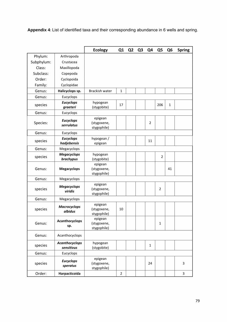
79  

Appendix 4: List of identified taxa and their corresponding abundance in 6 wells and spring.  

 

Ecology  Q1 Q2 Q3 Q4 Q5  Q6  Spring 

Phylum:  Arthropoda                         

Subphylum:  Crustacea    

Class:  Maxillopoda    

Subclass:  Copepoda    

Order:  Cyclopoida    

Family:  Cyclopidae    

Genus:  Halicyclops sp.  Brackish water  1                   

Genus:  Eucyclops    

species Eucyclops graeteri 

hypogean (stygobite) 

17           206  1    

Genus:  Eucyclops    

Species:  Eucyclops serrulatus 

epigean (stygoxene, stygophile) 

         2          

Genus:  Eucyclops    

species Eucyclops hadjebensis 

hypogean / epigean  

         11          

Genus:  Megacyclops    

species Megacyclops brachypus 

hypogean (stygobite) 

            2       

Genus:  Megacyclops epigean 

(stygoxene, stygophile) 

               41    

Genus:  Megacyclops    

species Megacyclops 

viridis 

epigean (stygoxene, stygophile) 

            2       

Genus:  Megacyclops    

species Macrocyclops 

albidus 

epigean (stygoxene, stygophile) 

10                   

Genus: Acanthocyclops 

sp. 

epigean (stygoxene, stygophile) 

            1       

Genus:  Acanthocyclops    

species Acanthocyclops 

sensitivus hypogean (stygobite) 

         1          

Genus:  Eucyclops    

species Eucyclops speratus 

epigean (stygoxene, stygophile) 

         24        3 

Order:  Harpacticoida     2                 3 

   

80  

Phylum:  Arthropoda                         

Subphylum:  Crustacea    

Class:  Ostracoda    

Subclass:  Podocopa    

Order:  Podocopia    

Suborder  Cypridocopina              

  

Superfamily  Cypridoidae              

  

Family  Cypridae    

Genus  Cypria    

Species Cypria 

ophtalmica 

epigean (stygoxene, stygophile) 

2     30  171        1 

Genus  Cypria   

Species Cypridopsis 

vidua 

epigean (stygoxene, stygophile) 

      1        1    

 Genus   Bradleycypris    

Species Bradleycypris 

obliqua 

epigean (stygoxene, stygophile) 

            6       

Phylum:  Arthropoda                         

Subphylum:  Crustacea    

Class:  Malacostraca    

Order:  Isopoda    

Family:  Sphaeromatidae              

  

Genus:  Sphaeroma. Sp.              1          

Family:  Gammaridae    

Genus:  Gammarus    

Species:  G. pulex  freshwater        1             

Genus:  Gammarus fresh/brackish 

water 2     9        3