A POSITIVE MODEL OF EXPENDITURE GROWTH: TOWARD CLOSURE OF

THE ORGANIZATIONAL PROCESS THEORY OF BUDGETING

DRAFT: Please do not quote or cite without permission

by

M.U. Dothan, Mike Hand, and Fred Thompson Atkinson Graduate School of Management and

Willamette Center for Governance and Public Policy Research Willamette University

900 State Street Salem, OR 97301 USA

Address all comments to fthompso@willamette.edu

ABSTRACT Optimal control theory and martingale methods are more elegant ways of modeling dynamic, stochastic processes than alternatives such as Monte Carlo simulation methods and equally powerful, but they are nevertheless rarely used in our field, due in part, perhaps, to their unfamiliarity. In this article we illustrate their power by completing one of the more compelling computational models of organizational process extant: the Crecine-Padgett model of the budgetary process. This model very accurately explains spending at the program or agency level in the period in which a budget is executed in terms of last year’s spending for the same purpose and revenue growth. But it lacks predictive power because its treats revenue change as an exogenous variable. Consequently, to close this model, a theory of revenue and/or aggregate spending growth that is endogenous to organizational process theories is needed. This article offers just such a theory for jurisdictions that face a hard budget constraint, using optimal control theory and martingale methods. This theory takes a jurisdiction’s existing revenue structure and its fiscal assets (savings) as given, and treats revenue and savings growth as continuous-time, continuous-state stochastic processes. This means that next year’s revenues and, thereby, funds available for spending can be predicted using current (in the period of budget formulation or enactment) state variables only. Combined with Crecine-Padgett model of the budgetary process, this means that we can predict and not merely explain spending changes at the program or agency level. Keywords: Process • Mechanism • Martingale methods • Optimal stopping models JEL Classification Numbers: H71 • H72

A POSITIVE MODEL OF EXPENDITURE GROWTH: TOWARD CLOSURE OF THE

ORGANIZATIONAL PROCESS THEORY OF BUDGETING

1 Introduction

In the standard economic model, public spending is determined by the demand (usually on the part

of the median voter) for and the supply of publicly provided goods and services. Consequently,

other things equal, the income of the median voter, the tax price of the service, and the size of the

jurisdiction determines spending levels. This model works exceptionally well for some purposes

and fairly well for many others. However, if what we seek is a budget theory that would “correctly

describe how it is that public funds are spent for one thing rather than another” (Key 1940: 1137),

the standard model is an exceedingly blunt instrument.

In contrast, organizational process theories of budgeting have achieved remarkable success

in explaining public expenditure outcomes at programmatic and departmental levels. The origins

of the organizational process theory of budgeting can be traced to the work of three prominent

scholars — Herbert Simon, Charles Lindblom, and Aaron Wildavsky (see especially Wildavsky

1964; Davis, Dempster, and Wildavsky 1966, 1974). The theory was articulated in its clearest and

most complete form in John P. Crecine’s 1969 book Governmental Problem Solving (Crecine

1969) and was elegantly formalized by John F. Padgett (1980, 1981). Indeed, one might well argue

that this body of work ought to be one of the most prominent milestones in analytic social science.

Crecine and Padgett distilled from an inchoate mass of “thick institutional detail” mechanism-

based models that provide “precise, abstract, realistic, and action-based explanations” (Hedström

Hedström 2005: 1) of public spending.

Yet, despite their rich provenance and notable successes, organizational-process theories of

government behavior have slipped into neglect, although thanks to the work of Kenneth Meier and

Laurence O’Toole (O’Toole and Meier 2011) they have garnered increased attention in recent

years (see also Bendor 1990, 2003; Green and Thompson 2001; Jones 2002, 2003; Dezhbakhsh,

Tohamy, and Aranson 2003; Tohamy, Dezhbakhsh, and Aranson 2006; Breunig and Koski 2006;

Robinson, Caver, O’Toole, and Meier 2007).1

Consequently, theorists have tended to revert to variable-based explanations of budgetary

outcomes in which an inertial component, combined with a standard set of macroeconomic,

political, and institutional indicators, explain spending outcomes (Su, Kamlet, And Mowery

1993).2 Or, they throw up their hands and declare that resource allocation decisions are not really

made through the budget process at all. Instead, budgets are merely an accumulation of

incremental adjustments – public-service bargains governing entitlements, employee salaries and

wages, service levels, and performance indicators – plus other matters that are only indirectly

related to the budget process but which are powerfully influential with respect to spending

outcomes and levels (see, for example, Patashnik 1996, for a compelling statement of this

perspective).3

There are several good reasons for neglecting organizational-process theories of budgeting

(Green and Thompson 2001). Their biggest flaw, however, is that they are woefully incomplete.

They explain spending at the program or agency level in the period in which a budget is executed in

terms of the previous year’s spending for the same purpose and total spending growth. What this

means that one must know how much revenue was deemed available to be spent overall in a period

(or, empirical analysis, was spent) before one can say how much spending would grow (or decrease)

1 This is especially regrettable because, in the period following the formulation of Crecine’s model, considerable progress was made toward a sophisticated understanding of the mechanisms and activities that influence the allocation of budgetary resources, which emphasizes the relative "controllability" of expenditure categories, transient preferences, and the stochastic effects of short-term expenditure solutions, see Downes and Rocke 1984, Bromily 1981, 2 As is the case with organizational-process budget models, these variable-based models usually lack predictive power because they too rely on variables from the period of execution rather than the period of formulation. Where their purpose is evaluating the consequences of discrete events (e.g., a change in budget rules or a disaster), this is not a drawback. But, of course, neither is it a drawback of organizational-process models when they are used for this purpose (see Larkey 1979).

for a particular purpose, function, agency, or department in that period. This is a remarkable

accomplishment, of course, but it leaves us with theories that lack any real predictive power.4

In other words, the fundamental flaw of organizational-process budget models is that they

treat total spending in the year of execution as exogenous to the model. Every version of the theory

starts with the presumption that budgets must be balanced against a spending constraint and that this

constraint is the principal driver of budgetary outcomes, but the formulation’s prime mover remains

a deus ex machina. The mechanism – a continuous chain of intentional and causal links through

which a global spending constraint is established – is never specified.

What the organizational process approach to budgeting lacks and, therefore, what it needs is

a mechanism that predicts global spending. More precisely, we want to predict how much budget

actors will choose to spend overall in the next future budget period, given uncertainty about both

future revenues and net savings, but complete knowledge about current relevant financial variables

and their volatilities. In this article, we propose a partial correction for this lack. We say partial not

only because ours is a first stab at a solution, but also because it applies to a limited subset of

governments, albeit an important one: our model is concerned only with governments that face a

“hard budget constraint.” A hard budget constraint means that these enterprises can neither force

central banks to buy their bonds nor expect a higher jurisdiction or authority to rescue them from

fiscal distress (Rodden, Eskeland, and Litvack 2003). Second, as a first approximation, our model

takes a government’s existing revenue structures and volatilities as givens.

3 Perhaps the best reason for rejecting this view is evidence that budgetary institutions affect spending outcomes (Wehner 2007; Anderson and Minarik 2006; Primo 2006; Alesina and Perotti 1996; Alesina et al. 1996). It is hard to square this finding with the claim that the budget process is itself irrelevant. 4

In several versions of the model (e.g., Crecine 1969), the spending constraint is referred to as a revenue constraint, which gives it specious proximity and materiality. Consequently, some students of the budgetary process have overlooked the incompleteness of the model (see, however, Choate and Thompson 1988; Davis, Dempster, and Wildavsky 1971, 1974; Downs and Rocke 1983, 1984).

2 The Model

To show that the budget actor’s global spending problem can be formulated with some precision

and to show how a computational solution to that problem can be found, we make two analytic

turns. First, we specify the aspirational purpose served by the budget process. This is necessary to

formulate the problem. Second, because the problem concerns an irreversible process that takes

place over time, in which the order in which actions and events take place affects their outcomes,

we embrace a set of powerful, new mathematical tools – optimal control and martingale theory –

that allow us to find precise computational solutions to problems involving dynamic processes like

this one. These methods are sufficiently developed that it makes sense to us to try to bring them to

bear upon the budget process.

At the risk of over-reaching, we start by making some sweeping statements about

aspirational purposes in general and those specific to government in particular. It is our position that

theoretical reasoning about the causal sources of events should adopt an enterprise view of the

processes we study. That is, we should try to understand them in terms of their aspirational

purposes. This is not an outré position. It is precisely how we study business, for example. We

usually start by assuming that businesses maximize net-present-value benefits to their stakeholders.

After about a century of debate, we have determined that this usually means maximizing the present

value of future free-cash flows thrown off by inventory turnover,5 which resolves the recognition

question (when to count performance), the standing question (whose benefits count), and the

question of idiosyncratic risk. We justify this norm by referencing Fisher’s separation theorem,

which argues that shareholders should care only about a business’s profitability and not the means

by which it is realized6 and the claim that shareholders ought to be indifferent to enterprise-specific

5This norm doesn’t apply to all businesses, banks, for example, create value by holding financial inventories; using equity, risk pooling, and hedges to manage inventory risk. It is not unreasonable to suggest that many of them got into trouble precisely because they lost sight of this purpose and instead got caught up in maximizing yields. 6This assumption seems self evident, but it isn’t necessarily valid. Shareholders often appear to have preferences for things other than the properties of a business’s returns. “Social responsibility” may be an example. A preference for

or idiosyncratic risk, because they can diversify it away. Then, once we have established a

satisfactory norm that can be used to discern appropriate action, we can, where there is reason to do

so, investigate the consequences of conditions that are intrinsic to the situation at hand: asymmetric

information, bounded rationality, peculiar business strategies, path dependencies, or shifting

internal coalitions.

It seems strange to us that where government is concerned our colleagues all too often fixate

on intrinsic issues rather the pursuit of aspirational purpose. Even general-purpose formulations

such as Niskanen’s revenue maximization seem to be motivated by desire to explain a particular

defect or malfunction. Resolution of these kinds of issues often has little instrumental utility,

unfortunately. If you cannot say what success looks like you cannot say much about anything else

of importance.

For example, we are fans of Dan Carpenter’s writings, especially his most recent book,

Reputation and Power: Organizational Image and Pharmaceutical Regulation at the FDA (2010).

His is, perhaps, the best work about the performance/behavior of government programs being done

now and some of the best ever done. What we especially like about this book is its use of real

options analysis. Carpenter assumes that safety is a continuous-time Wiener process, with an

absorbing barrier at zero. Carpenter further assumes that time and repeated drug trials will allow the

FDA to learn. Finally, the value Carpenter assigns to the FDA’s aversion to adverse drug reactions

drives the model’s optimal stopping point. This is a typical problem of administrative choice. Many,

if not most, administrative choices can and probably should be modeled as learning problems.

Consequently, this approach has a great deal of instrumental merit.

But we are uncomfortable with his analytical strategy, which presumes a highly

idiosyncratic objective function for the FDA: maximizing agency reputation. How reputation or

profitable fast-growing businesses (growth stocks) is probably a better one. That some investors get utility from owning these stocks (being connected to a “winner”), although they tend to be poorer investments than value stocks, is one possible explanation for the anomalous market premium they command.

even political influence adds to our understanding of the timing of FDA approvals seems like a

secondary question. We are not denying that this question has intellectual bite.7 But, putting it first

seems like a case of the tail wagging the dog.

If the FDA were a straightforward analog to a business enterprise, we would probably begin

our research with the presumption that it maximizes performance in terms of net health benefits

from proposed new pharmaceuticals, which can be measured in terms of effects on patients’ quality-

adjusted life years, a measure that combines health status and years of health. This formulation is

directly analogous to business purpose because, while it offers answers to the recognition and

standing questions more appropriate to the case at hand, it focuses on net-benefit maximization.

Furthermore, this purpose also provides a counterfactual against which the consequences of self-

interested behavior on the part of agents, conformity to political pressures, unthinking habit, or the

stream of influences from the environment can be assessed.

Increasingly, however, we have become convinced that net-benefit maximization and a

fortiori risk neutrality profoundly misconceive the fundamental purpose of government. The

aspirational purpose of government in a commercial republic is not performance maximization; that

is, in fact, secondary. Its main aspirational purpose is stability.

Why should stability be especially important for governments? The answer goes to their

core purposes. Think about the words commonly used to talk about public purposes: safety,

reliability, guarantee, order, and security, even the FDA’s purpose is expressed in terms of insuring

the safety as well as the efficacy of new drugs. All of these terms go to the mitigation of systemic

and idiosyncratic risk. As Tony Judt put it, we “have to have active interventionist states protecting

us against things that frighten people” (Judt and Božić 2010:11).

Certainly, much of what government does seems to be designed to bring about order in what

would otherwise be chaotic: standard setting, coordinating networks and the like. Even more of it

7On further reflection, it occurs to us that these issues might be of instrumental interest to a political scientist, which is

looks like insurance: tracking and incapacitating threats, reducing individual vulnerabilities, and

moderating the consequences of adverse events, in other words, investing in before-the–fact

measures to improve risk preparedness, risk pooling and activity diversification, and providing

programs for recovery and reconstruction after the fact. Further, we accept that the functions

government enterprises perform are things that we cannot do without, although, over time, as we

become richer, we expect government to confront ever more distant, more intractable risks (Shiller

2003; Hacker 2007).

Does this statement about aspirational purpose allow us to make interesting, surprising

causal or instrumental claims about the processes we observe? Yes. If stability is central to

government enterprises, their master decision-making arrangements: the budget process and

machine bureaucracy, make a lot of sense, where otherwise they might not, as do the extreme

measures often taken by public officials to stabilize service delivery, such as cutting back on

maintenance. Maintenance can be deferred, at a cost, many government operations can’t, they must

be provided in real time, and the organizations that conduct them cannot be permitted to fail (in the

sense of shutting down when needed).

Moreover, this formulation implies a fairly straightforward set of causal linkages from

politics to public policy (Douglas & Wildavsky 1982). On the left, Judt (Judt and Božić 2010:11):

“proposes a social democracy of fear…. Why not face up to this challenge in the name of a

progressive state with collective objectives and purposes, which preserves institutions that give us a

sense of shared identity and values? We are going to have to find a new language in which to

express the role of the state in this uncertain world.” Or, on the right, conservatives like David Frum

(1994: 4) emphasize that richer is usually safer and express concerns with the consequences of

social insurance – moral hazard and adverse selection:

what Carpenter is.

The great, overwhelming fact of a capitalist economy is risk…. Risk makes people circumspect. It

disciplines them and teaches them self-control. ... Without welfare and food stamps, poor people

would cling harder to working-class respectability than they do now.

All of this suggests an objective function for government enterprises, which looks something

like the following: minimize risk, subject to revenue and service accomplishment or delivery

constraints. One further intellectual advantage of this formulation – government mitigates risk,

business maximizes return – is that it unambiguously distinguishes public from private enterprises.8

Having once accepted this broad statement of purpose, existing models from financial

economics (Dothan 1990) can be reformulated in a straightforward manner to represent the budget

actor’s global spending problem. A hard budget constraint provides budget actors with an

intentional problem: stabilizing service deliveries in the face of revenue uncertainties, largely a

function of the business cycle; an opportunity: to save for a “rainy day,’ and even an enforcement

mechanism constraining their choice set: the debt market (Lowry 2001). At a minimum, reliance on

independent debt markets means that budget actors must persuade lenders that the present value of

their jurisdiction’s future revenues plus net savings (financial assets minus financial liabilities) are

equal to or greater than the present value of their future spending (Buiter 1990: 63-7).9 In financial

economics, it is easy to show there is an optimal solution to the present-value spending problem,

which is the key to budget actor’s global spending problem, given a hard budget constraint.

Actually solving the budget actor’s global spending problem in real time, especially from

one period to the next, is much harder computationally, even where the problem can be formulated

in a straightforward manner, as we think it can be here.

2.1 The Mechanism

8This means they can often be more efficiently financed by a jurisdiction than by individuals. Fire departments, for example, protect us from fires that might otherwise threaten get out of control, destroying whole neighborhoods or even cities. Consequently, they are nearly everywhere supported by mandatory levies, often property taxes, even where the services are provided by competitive businesses, as in Denmark, for example.

Mechanisms are the constructs we use to explain why processes turn out the way they do.

For example, evolution is a process; natural selection is one of the mechanisms that determine its

outcome. Similarly, budgeting is a process and balancing and precedent are among the mechanisms

that determine its outcome. Real processes take place over time. Consequently, where real processes

are concerned, mechanism-based explanations look like algorithms or, perhaps, scenarios, when the

analytical tradeoff tilts away from abstraction toward veridical realism. Indeed, it is necessary for

most of us to hear a credible back-story before we will accept an abstract model as satisfactory

representation of a process. In this case, the back-story has budget actors, in Crecine’s words,

“organizational decision-makers and problem solvers who structure complex problems, generate

alternatives, and make choices” (Crecine 1969: 20), making global spending decisions subject to a

present-value constraint and considerable uncertainty about future cash inflows.

Analytically speaking, the question is how best to deal with the uncertainty facing the

budget actor? Like Padgett (1981) and George A. Krause (2003), we choose to formalize

conditions, which for reasons of purpose and method Crecine leaves tacit and open-ended, although

our efforts to understand budgetary decision making under uncertainty have more in common with

standard financial models than theirs. The way we do this is to treat the budget actor’s problem as a

particular kind of closed-form, stochastic-choice problem called an optimal stopping problem.

Stopping problems can be laid out two ways: deciding how long to wait before choosing (e.g.,

Carpenter 2010) or making the best stochastic choice possible at a specified time. In this instance,

both interpretations do some injury to reality. But the latter, setting a global spending level

according to a predetermined schedule, seems to fit the stylized facts of the budget formulation

process somewhat better than the alternative of deciding how long to delay before setting a global

spending level. Budget actors are usually described as making global spending decisions in the

9 More precisely, Willem Buiter expresses the solvency constraint of a jurisdiction subject to the "no-Ponzi game" condition as: PV of exhaustive spending ≤ {(assets – debts) + PV (taxes – transfers)}, where PV denotes the present

period of budget formulation and then sequentially repeating this process in each subsequent period

of execution (when the spending occurs), basing future spending levels on the expected outcomes of

their choices and current state variables in the period in which the budget is formulated (Penner and

Steuerle 2004). Hence, we are saying that the budget actors’ problem is to determine an endogenous

optimal expenditure process xt, given a budget savings or reserve account, Ht, subject to the binding

constraint that the risk-adjusted present value of future spending must be equal to or less than net

financial savings, Ht, plus the risk adjusted present value of future revenues.

Finally, one of the characteristics of deterministic optimal stopping problems is that actors’

preferences, especially their risk preferences, drive their results. Consequently, “criteria must be

advanced that can enable scholars to empirically demarcate between risk–aversion, risk–neutrality,

and risk–seeking behaviors” (Krause 2003: 171). Here, we assume that budget actors have a utility

function over the spending stream discounted by the combined value of population growth and

inflation and we denote this combined growth rate by α, constant relative risk aversion γ and rate of

time preference φ. Other relevant state variables are the market price of risk, which we denote by

θ, the risk-adjusted capitalization rate of revenue, denoted by k, and the interest rate paid on

savings (assumed to be invested in bonds), denoted by r.10

The assumption that a government’s existing revenue structures and volatilities are givens

can be formalized as meaning that the entity’s revenue stream yt is exogenous to the model and its

dynamics, over very short time intervals, dt are the sum of constant growth at rate µ and a random

shock represented by an increment of Brownian motion Bt, a continuous-time symmetric random

walk whose increments have normal distribution with zero mean and variance t, scaled by a

volatility parameter σ.

value of a cash flow. 10 We assume that, so long as a jurisdiction avoids Ponzi finance, it can lend or borrow at the same rate.

The specification of revenue dynamics in Equation (1) implies the following revenue stream:

The random revenue process in Equation (2) is called exponential Brownian motion and is

characterized by an infinite number of potential sample paths with intermittent periods of

exponential growth and decay. At any future time, the distribution of exponential Brownian motion

is log-normal.

2.2 Optimal Spending

To find the solution to the budget actors’ problem, we exploit an analogy between

government expenditures and investor’s consumption, and between government revenues and

investor’s labor income. Merton (1971) solved an optimal consumption and portfolio problem for

an investor with no labor income, using continuous-time dynamic programming. We modify

Merton’s problem to include random government revenue whose dynamics are represented by an

exponential Brownian motion. We assume that financial markets are rich enough to allow hedging

the uncertainty in future government revenue, but that legal and institutional factors restrict the

government to implementing the optimal expenditure policy through investing the reserve account

in risk-free bonds only or, if the reserve account is negative, borrowing at the risk free rate. With

that assumption, the solution of the actor’s problem is given in Equations (3) and (4).

Equation (3) says that optimal expenditure is a constant fraction V of wealth, defined as the value of

the reserve account (which could be negative as well as positive) plus the risk-adjusted present

value of future revenues. The fraction V represents the optimal spending rate from wealth, and

remains constant through time and is given by

It may seem somewhat counterintuitive, but the model implies that budget actors with low

levels of risk aversion would save a lot (make substantial investments in the reserve account).

Moderately risk-averse budget policy makers would tend to spend more and save less (invest less in

the reserve account). Very high levels of risk aversion, however, would cause them to reduce

spending and increase savings. This pattern of spending and saving is analogous to the conflicting

influences of substitution and income effects. On one hand, increased risk aversion causes actors to

substitute saving for spending, but, because risk aversion causes them to “feel poorer,” they spend

more and save less. Our model says that the income effect dominates the substitution effect at

moderate levels of risk aversion, and that the substitution effect dominates the income effect at

higher levels of risk aversion.

Table 1 presents the comparative statics of optimal spending from wealth V. We assume a

base case with parameter values r = 5%, µ = 7%, σ = 10%, α = 4%, φ = 0%, γ = 5, θ = 0.45, and k =

9.5%. Table 1 shows that in the base case optimal spending is 2.42 percent of wealth. Increasing

bond rate r, time preference φ, and market price of risk θ from base-case values increases spending.

Increasing growth α and risk aversion γ from base-case values reduces spending. Other things

equal, changes in expected long-run growth of revenue and long-run volatility of revenue would

have no effect on spending rates (expressed as a proportion of wealth V). However, because an

increase in revenue growth α increases wealth V, increased revenue growth would also allow higher

spending levels. Similarly, an increase in the long-run volatility of revenue would likely reduce

wealth by increasing the market price of risk θ.

Equation (4) describes the optimal value of the reserve account as a function of the history of

revenue ys for 0 ≤ s ≤ t. Because our analysis is in continuous time, our formula reflects

continuous compounding of the reserve account at the annual rate r. The formula follows by

integration from the compounding equation, where xt is given by Equation 3. Recursive

calculation using Equation (6) represents a very good approximation to Equation (4) when Δt is

one day or less.

2.3 Optimal Reserve Account

To investigate the optimal size of the reserve account Ht it is convenient to consider the optimal

reserve to revenue ratio Ht / yt. From Equation (4) we can compute this expected ratio when time

goes to infinity Table 1 also shows the comparative statics of this ratio. In the base case, the optimal

long-run expected reserve account is 93.57 percent of annual revenue. Compared with that case,

increasing bond rate r, revenue volatility σ, combined growth rate α, budget actor’s risk aversion γ,

and market price of risk θ increase the size of the long-run optimal reserve account. Increasing

expected long-run growth of revenue µ reduces the size of the optimal reserve account and may

even convert it into a debt account, as in row 3 of Table 1.

Similarly, although less happily, changing actors’ time preference φ in our model so that they prefer

near-term spending to future spending, also reduces the size of the reserve account, as in row 6 of

Table 1, and, if the increase in φ is large enough, could convert it to a debt account. Of course, a

good positive model of the budget process should explain avoidable financial distress and not

merely desirable outcomes (Holcombe and Sobel 1997; Hou 2006).

2.4 Spending from Revenue and the Optimal Surplus

Equations (3) and (7) imply that the optimal long-run ratio of spending to revenue is as shown in

Equation (8). In turn, Equation (8) can be rearranged to show the long-run optimal ratio of spending

to the long-run optimal ratio of surplus to revenue, Equation (9).

Figure 1 illustrates the optimal spending rate from revenue at a fixed time t as a function of the

relative risk aversion γ of budget policy makers for three different values of combined growth α,

where the other input parameters are: r = 5 percent, µ = 7 percent, σ = 10 percent, φ = 0 percent,

θ = 0.45, k = 9.5%, Ht = 0, and yt = 100. What Figure 1 shows is that risk aversion implicitly

presumes a higher future rate of growth in spending and, therefore, requires an increase in the

current surplus or a reduction in the current deficit. Again, a good positive model of the budget

process should explain avoidable financial distress and not merely desirable outcomes.

Figure 1. Optimal Spending Rate from Revenue

3 Empirical Assessment

Hedström reminds us that while statistical analysis is not explanation, it is “important for testing

proposed explanations” (2005 23). So, how well does our model do? The answer to that question

depends, of course, upon the specification tested and the analytical alternatives. In this case, we

have a fully identified model. Consequently, it would be possible, given sufficient resources, to

predict spending levels and reserves for any jurisdiction and time period with considerable

precision, using normative standards for risk aversion and time preferences (see Dothan &

Thompson 2009a, 2009b), to generate an appropriate counterfactual. We could then employ 2SLS

to estimate actual values for those parameters.

Alas, we lack the resources needed to carry out this analysis. As a result we have adopted a

less satisfactory expedient, employing an incomplete specification, aimed at justifying the

underlying assumptions of our model, primarily the assumptions that reserves (H) depend upon

revenue volatility (σ) and revenue growth (µ). Given Equation (6) and assuming current state

variables are held constant (which is counterfactual, but it ought not bias our results if we treat their

effects as noise), the model implies

Δ Ht = f (σ0 ) (10)

Δ Ht = g (µ0 ) (11)

This prediction is surprising only to someone who holds that government spending is perverse

Test 1

We used the following OLS model to measure the determinants of expected municipal

savings (fund balances):

ln(SAVINGS/EXPENDITURESit) = α0 + α1CV REVENUEit + α2DEBT PER-CAPITAit-1 + α3LIMITED REVENUE + α4SIZEit + α5GROWTHit + α6STATE REVENUEit + ΣαkFYEk + ΣαmSTATEm + ΣαtYEARt

(12) where i represents the ith government entity and t represents the year of observation. SAVINGS/EXPENDITURES is the ratio of fund balances to monthly operating and interest

expenditures; CV REVENUE is the coefficient of variation of revenue, defined as the ratio of the

standard deviation of revenue to mean revenue, measured over the previous four years (proxy for

revenue uncertainty); DEBT PER CAPITA is total debt/total population (inverse proxy for revenue

uncertainty); LIMITED REVENUE is a revenue diversification index, or (r1/R)(r2/R)…(rN/R), where

r is the amount of revenue received from a specific source, and R is total revenue (proxy for revenue

uncertainty); SIZE is the log of total population; STATE REVENUE is the total state revenue

received/total revenue (inverse proxy for revenue uncertainty); GROWTH is the change in revenue

from year t-5 to t, deflated by population in year t (proxy for revenue uncertainty); FYE is a series

of dummy variables indicating the quarter of the fiscal year end; STATE is a dummy variable

indicating the state; and YEAR is a dummy variable indicating the year.

SAVINGS/EXPENDITURES are computed as total fund balances (or fund equity) at the end of

each fiscal year, deflated by total expenditures per month, which includes operating and interest

expenditures, which represents the number of months governments can operate without collecting

revenue. Because of dramatic disparity in the savings to expenditure ratios, ranging in value from 0

to 6336 with coefficient of skewness = 67.6, the natural log of this ratio was employed as the model

response.

Data are from the Census Bureau's Annual Survey of Governments for all cities, towns,

boroughs, and villages in the database (Government Type = ), covering nearly 20,000

municipalities. Required financial measures are extracted from Government Finance Statistics,

Individual Unit Files and matched against Government Integrated Directories for population and

other entity attributes. The Individual Units data contain details for all “income statement” accounts,

including revenues, expenditures, and transfers. The Census files also provide “balance sheet” data

such as cash and debt. The sample period covers the years 1992 and 1995 – 2006, all years for

which Individual Unit Files are currently available.

Summary statistics for model variables are displayed in Table 2 and the results of the model

analysis are reported in Table 3.

TABLE 2: Summary Statistics for Model Variables

Variable n Mean Median Std Dev Minimum Maximum

Savings/Expenditures 80,150 13.0830 8.0000 44.6112 0.0000 6,336.0000

ln (Savings/Expenditures) 75,121 2.0947 2.1511 1.0146 -5.4810 8.7540

CV Revenue 16,634 0.1418 0.0998 0.1482 0.0000 2.0000

Debt Per Capita 80,928 2.6846 0.6825 33.5217 0.0000 3,709.4600

Limited Revenue 77,670 0.0001 0.0000 0.0017 0.0000 0.0370

Population 81,023 20,863 2,123 133,149 0 8,214,426

Size = ln (Population) 81,023 7.8278 7.6611 2.0570 0.0000 15.9214

Growth 41,979 0.0149 0.0049 0.5251 -0.1985 104.4500

State Revenue 80,335 0.1661 0.1170 0.1643 0.0000 1.0000

TABLE 3: Determinants of Municipal Savings *, **, *** indicate significance at p <.10, .05, and 01; based on two-tailed tests.

Variable Coefficient Std Err t-Stat Significance

Intercept 1.1415 0.3022 3.7773 0.0002 ***

CV Revenue 0.2327 0.0728 3.1945 0.0014 ***

Debt Per Capita -0.0002 0.0001 -1.8804 0.0601 *

Limited Revenue 12.2001 3.7555 3.2486 0.0012 ***

Size = ln (Population) -0.0192 0.0061 -3.1669 0.0015 ***

Growth 1.9494 0.1870 10.4224 0.0000 ***

State Revenue -0.3012 0.0880 -3.4209 0.0006 ***

FYE Quarter Indicators Included1 ***

Year Indidcators Included1 ***

State Indicators Included1 ***

Adjusted R2 0.238

1For brevity, the quarter-specific, year-specific, and state-specific intercept terms are not reported.

Fiscal year-end, state, and year indicators are included in the regressions, but are not reported in

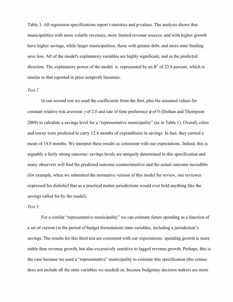
Table 3. All regression specifications report t-statistics and p-values. The analysis shows that

municipalities with more volatile revenues, more limited revenue sources, and with higher growth

have higher savings, while larger municipalities, those with greater debt, and more state funding

save less. All of the model's explanatory variables are highly significant, and in the predicted

direction. The explanatory power of the model is represented by an R2 of 23.8 percent, which is

similar to that reported in prior nonprofit literature.

Test 2

In our second test we used the coefficients from the first, plus the assumed values for

constant relative risk aversion γ of 2.0 and rate of time preference φ of 0 (Dothan and Thompson

2009) to calculate a savings level for a “representative municipality” (as in Table 1). Overall, cities

and towns were predicted to carry 12.4 months of expenditures in savings. In fact, they carried a

mean of 14.8 months. We interpret these results as consistent with our expectations. Indeed, this is

arguably a fairly strong outcome: savings levels are uniquely determined in this specification and

many observers will find the predicted outcome counterintuitive and the actual outcome incredible

(for example, when we submitted the normative version of this model for review, one reviewer

expressed his disbelief that as a practical matter jurisdictions would ever hold anything like the

savings called for by the model).

Test 3

For a similar “representative municipality” we can estimate future spending as a function of

a set of current (in the period of budget formulation) state variables, including a jurisdiction’s

savings. The results for this third test are consistent with our expectations: spending growth is more

stable than revenue growth, but also excessively sensitive to lagged revenue growth. Perhaps, this is

the case because we used a “representative” municipality to estimate this specification (the census

does not include all the state variables we needed) or, because budgetary decision makers are more

myopic and/or risk averse than we assumed.

Test 4

` Don Boyd suggested another reasonable alternative approach to assessing this model when

he observed “the public part of revenue forecasting is a short game – forecasting the remainder of

the current year plus the year ahead.” Budget actors, he concludes, focus on the short game and can

certainly do better than by assuming revenue is a random walk. “For example, in the typical state

with an income tax, a revenue forecaster in February or March knows at least a little bit about the

current tax year – a calendar year – and virtually all of the payments on that tax year will be made

by the time returns are filed a year hence in April.” (Boyd 2007)

To properly identify our model we should take into account all the current (t = 0) state-

variables laid out in Equations 3 and 7. Then, perhaps, by matching observed spending with

estimated spending using Monte Carlo simulation and a truncated data set, we could specify the

values of the risk and time preference variables. Finally, we could use an expanded reduced-form

model and the reserved observations to test the predictive power of this model.11 In the meantime,

we offer the following reduced-form specification as a crude approximation of that ideal: given the

validity of Equation (5) and assuming current state variables are held constant (which is

counterfactual, but it ought not bias our results if we treat their effects as noise), the model implies

Δ Xt = f (µ0 ) (13)

Equation (13) can be estimated using the following empirical model, where t = 0 is the period in

which the budget is formulated and t = 1 is period in which the budget is executed.

log x1 – log x0 = α + β (µ0) + ε (14)

11 Note, we have not done this. But, if the main objection to our argument goes to our admittedly casual empirical results, it would probably be feasible to do so, although collecting the necessary historical data would not be easy. Actually, this is another reason for the neglect of organizational process models – testing them requires vast amounts of historical data of kinds that can be recovered only with the greatest difficulty (Green and Thompson 2001).

In contrast, Boyd’s description of revenue forecasting implies something like the following:

Δ x1 = f (ρ0 ) (15)

where ρ = the revenue forecast upon which the spending plan is based. Presumably, Equation (15)

can be estimated using the following empirical model, where ψ = the estimated revenue for the

period in which the budget is formulated.

log x1 – log x0 = α + β (log ρ1 - log ψ0 ) + ε (16)

To estimate these models, we used Oregon state revenue and spending data (not counting rebated

taxes) for 1960-2001.12 Next, we decomposed the historical data into two components: a trend and a

random component. The trend is simply the mean of past growth rates (where revenue is concerned,

µ in our model). The random component is the variance. The variance is the average of the squared

differences between actual growth rates and the mean growth rate – or mean squared error. The

standard deviation of the distribution is simply the square root of the variance (where revenue is

concerned, σ in our model). The revenue trend was 7.40 percent, with a standard deviation of 9.80

percent; the spending trend was 7.14 percent (not counting rebated taxes), with a standard deviation

of 8.37 percent. To simulate the change in µ from one year to the next, we assigned the mean

growth rate to t = 1 (1960), so that µ1 = 7.4 and estimated the mean growth rate for t = 2 (1961) as

µ2 = (log y2 – log y1) 1/e

+ µ1

1-1/e, and repeated that process through t = 40 (2000), so that µ40 = (log

y40 – log y39)1/e + µ391-1/e.

Estimating Equations (14 & 16) via OLS regression, we obtained β = 1.1289, R2 = .272, F =

12 We used Oregon state revenue and spending data because we had them on hand for another purpose. Unfortunately, the data, especially the spending data, from earlier than 1977 are neither consistent nor very reliable. Moreover, one year was completely missing from the data set. Nevertheless, Oregon is a good case with which to test our model, because the state’s revenue structure has been stable for over forty years and because, although Oregon’s Constitution requires the enactment of a balanced budget, it does not require current spending to be equal to or less than current revenue from operations plus fund balances (Poterba 1995). Also, Oregon formulates and enacts its budget for the following biennium using a revenue forecast that is announced six months before the start of the period of execution.

18.46 with 34 df, for the former and β = .135, R2 = 0.059, F = 1.1743 with 22 df, for latter. While

neither of these result sets is anything to write home about, the first is equal to or greater than the

first difference results reported by Davis, Dempster, and Wildavsky (1971, 1974; see also

Dezhbakhsh, Tohamy, and Aranson 2003) and provide confirmation that we are not merely building

castles in the air.13 The remarkable thing about the predictive power of Equation (14) is the

cumulative role of revenue growth reflected in global spending changes. According to Crecine,

precedent means taking past solutions and modifying them in the light of changes in available

information and current exigencies to obtain this year’s solution (Crecine, 1969, 41), which is

approximately what we see here.

These results also recapitulate Padgett’s (see also Downes and Rocke 1983) observation that

that “the apparent success of determinants models is largely attributable to the autoregressive

implications of focusing on absolute expenditure levels rather than changes” (1980: 360). Again,

following Padgett, we are inclined to believe that a better test of our model would focus on

examining distributions of changes rather than attempt to predict the magnitude of changes, but we

haven’t taken that step.

4 Conclusions and Discussion

In this case we have tested a model, which presumes that budgeting is a purposeful

enterprise, aimed at an identifiable normative optimum. The logic of our specific formulation

reflects the commonplace observation that the goal of this process is the stability of the fiscal

system. The things that government does, the services it provides have one fundamental attribute:

they are all things everyday people depend upon to get by – the legal system, incapacitating

criminals and fire protection, education, a transportation network, a social safety net, clean water,

etc. Moreover, deferring their delivery is often prohibitively costly; these services must be provided

13 We should acknowledge here that Boyd (2007) performed a similar exercise using Illinois data and apparently got a

in real time. That means their providers cannot be permitted to fail (in the sense of going out of

business, hence not being there when needed). The essential requirement for meeting this objective

is stable support. Hence, we formulated an objective function for the budget in terms of maximizing

stability or sustainability. We are not, in fact, surprised that the model’s predictions have been

confirmed. We expect our institutions to perform.

The next step is specifying a fully identified version of this model, not merely testing

inferences from the model, even counterintuitive as one,

As a practical matter, we know that the participants in the budget process don’t use

optimizing models that look like ours. Modeling the budget process as a set of differential equations

is no more than an analytic convenience aimed at showing what their behavior would look like if

they did optimize performance. Having found that their behavior is consistent with the predictions

of our model, the next question is what are the actual heuristics, decision rules, or mechanisms them

employ to produce this outcome

Ultimately, we would like to build a robust and sophisticated mathematical representation of

bounded, collective rationality along the lines of Padgett’s model of Federal budgetary decision

making in which the process of setting global spending targets was entirely endogenous.

Presumably, a more realistic model would incorporate taxing decisions and feature constrained

search routines, stochastic generation of alternatives, and probabilistic serial judgments, as well as

risk aversion. That is still a way off.

Perhaps a more realistic next step in developing an organizational-process model of overall

spending would be to provide the thick institutional detail needed to chart the flow of decisions that

go into setting tax and spending levels. By this, we mean identifying the principal actors and the

parts they play in the process and specifying the process flow algorithms used to decompose the

similar result for a specification like Equation (14), but a far better result for a specification like Equation (16) than did

taxing/spending problem into a set of manageable sub-problems. We would also like to identify the

devices that that have been improvised to reduce the complexity of setting tax and spending levels

to manageable dimensions. The process undoubtedly begins simply enough with basic financial

constructs and variables, but probably quickly increases in complexity.

For example, we would be greatly surprised if the average of past revenue growth rates were

not in general the best estimator of expected growth rates, but demographic and inflation trends are

probably somehow taken into account in setting global spending targets. We tried to factor this

variable into our model with α. But, exogenous events can be expected to influence spending

choices and inflationary and demographic surprises occur and probably fall into this general

category. Similarly, revenue growth above the trend and especially prolonged periods of above

trend growth may lead to different processes and decision-making heuristics than below trend

growth. Where revenue plus budget reserve accounts or savings (fund balances, rainy-day funds,

etc.) are insufficient to stabilize spending growth, what do the principal actors do? Or, more

correctly, who does what and why? Most of the organizational process literature implies that if tax

revenues are insufficient, budget actors start cutting – reducing the uses of cash, which from an

accounting standpoint is a source of cash. But there are other sources of cash. Asset sales are one

source; borrowing is another; new taxes a third. What determines the order in which these sources

are tapped? The cost of debt may not be the principal determinant, since funded debt appears to be a

lot cheaper than borrowing from fiduciary or investment funds or suppliers and, for the most part,

governments can borrow at lower rates than citizens, but that may be a misperception.

It is also hard to distinguish some kinds of borrowing from cost cutting – postponing

maintenance and cost-of-living adjustments or merit salary increases, for examples. Moreover, by

definition, jurisdictions facing hard budget constraints cannot expect a higher level of government

we. Unfortunately, he didn’t report his R2s or show the plots of his second set of estimates.

to rescue them from fiscal distress, but in many cases they can shift their problems to lower levels,

which seems rather like taxing. Also, we have implicitly assumed a unitary budget actor. However,

various participants in the process may have distinctly different time and risk preferences, which

induces a need for conflict-resolution mechanisms (Paleologou 2006). Here, we suspect that

computer simulation based on algorithms developed from carefully constructed decision-making

protocols might be very helpful in untangling this complexity.

We also suspect the general public management research community would be interested in

extensions of our model illuminating the roles that public financial managers and other

administrative professionals play in shaping its key elements. For instance, how, if at all, do public

financial managers and administrative professionals influence elected officials’ risk preferences or

time preferences? Do they have any influence over how governmental entities actually determine

expected revenues or the order in which sources of cash are tapped? Incorporating this sort of

administrative behavior into our model might be a very useful contribution to both traditional

budget theory and our understanding of public management. Nevertheless, it is impossible to say, a

priori, where or how far we ought to go in search of greater realism, at least, not with any certainty.

Ultimately, the question resolves to a matter of instrumental value – the proof of the pudding is in

the eating.

References

Alesina, A. and R. Perotti. 1996. Budget Deficits and Budget Institutions. NBER WorkingPaper

5556.

Alesina, A., R. Hausmann, R. Hommes, and E. Stein. 1996. Budget Institutions and Fiscal

Performance in Latin America. NBER Working Paper 5586.

Andersen, S.C., and P.B. Mortensen. 2010. Policy Stability and Organizational Performance: Is

There a Relationship? Journal of Public Administration Research and Theory 20(1): 1-22.

Anderson, B. and J. J. Minarik. 2006. Design Choices for Fiscal Policy Rules. OECD Journal on

Budgeting 5(4): 159-208.

Bardach, E. (2004) The Extrapolation Problem: How Can We Learn from the Experience of

Others? Journal of Policy Analysis and Management 23: 205-220.

Bendor, J. 2003. Herbert Simon: Political Scientist. Annual Review of Political Science 6: 433-471.

Bendor, J. 1990. Formal Models of Bureaucracy: A Review. In Public Administration: The State of

the Discipline, ed. Naomi Lynn and Aaron Wildavsky. Chatham, NJ: Chatham House

Publishers Inc.

Boyd, Donald J. 2007. Theory to Practice: Comment on Revenue Forecasting, Financial Theory,

and Budgets. PAR (online) 67/5 (September-October): 67-73. Accessed 1 Sep. 2007 at:

http://www.aspanet.org/scriptcontent/index_par_t2p_commentary.cfm

Breunig C., C. Koski. 2006. Punctuated Equilibria and Budgets in the American States. Policy

Studies Journal 34 (3), 363–379.

Bromiley, Philip. 1981. Task Environments and Budgetary Decision Making. The Academy of

Management Review 6 (2), 277-288

Bromiley, Philip, and John P. Crecine. 1980. Budget Development in OMB: Aggregate

Influences of the Problem and Information Environment. The Journal of Politics 42, (4),

1031-1064.

Buiter, Willem, 1990. Principles of Budgetary and Financial Policy. Cambridge MA: The MIT

Press.

Carpenter, D. 2010. Reputation and Power: Organizational Image and Pharmaceutical

Regulation at the FDA. Princeton: Princeton University Press.

Carpenter, D. 2003. Why Do Bureaucrats Delay? Lessons from a Stochastic Optimal Stopping

Model of Agency Timing, with Applications to the FDA,” in Politics, Policy, and

Organizations: Frontiers in the Study of Bureaucracy, George A. Krause and Kenneth J.

Meier (editors), Ann Arbor: University of Michigan Press, 2003: 23-40.

Choate, G. Marc and F. Thompson. 1988. Budget Makers as Agents. Public Choice 58/1: 3-20.

Crecine, John. 1969. Governmental Problem Solving. Chicago: Rand McNally & Company.

Davis, Otto A., Murray A. H. Dempster, and Aaron Wildavsky. 1974. Towards a Predictive

Theory of Government Expenditure: US Domestic Appropriations. British Journal of

Political Science 4: 419-452.

Davis, Otto A., Murray A. H. Dempster, and Aaron Wildavsky. 1971. On the Process of Budgeting

II: An Empirical Study of Congressional Appropriations. In Studies in Budgeting, ed. R. F.

Byrne and et al. Amsterdam: North Holland.

Davis, Otto A., Murray A. H. Dempster, and Aaron Wildavsky. 1966. A Theory of Budget

Process. American Political Science Review 60: 529-547.

Dezhbakhsh, Hashem, S.M. Tohamy, P.H. Aranson. 2003. A New Approach for Testing

Budgetary Incrementalism. The Journal of Politics 65 (2): 532–558.

Douglas, M., and Aaron Wildavsky. 1982. Risk and Culture: An Essay on the Selection of

Technical and Environmental Dangers. Berkeley: University of California Press.

Downs, George W. and David M. Rocke. 1984. Theories of Budgetary Decision making and

Revenue Decline. Policy Sciences 16: 329-347.

Downs, George W. and David M. Rocke. 1983. Municipal Budget Forecasting with Multivariate

ARMA Models. Journal of Forecasting 2: 377-387.

Dothan, M.U. 1990. Prices in Financial Markets. New York: Oxford University Press.

Dothan, M.U., and F. Thompson. 2009a. A Better Budget Rule, Journal of Policy Analysis and

Management 28(3): 463-478.

Dothan, M.U., and F. Thompson. 2009b. Optimal Budget Rules: A Proof, Given a Random Walk

with Drift. Public Finance and Management 9(3): 439-469.

Frum, David. 1994. Dead Right. New York: Basic Books.

Gist, John R. 1974. Mandatory Expenditures and the Defense Sector. Beverly Hills: Sage.

Green, Mark, and F. Thompson. Organizational Process Models of Budgeting, Research in

Public Administration. (2001) 7: 55-81.

Hacker, Jacob S. 2007. The Great Risk Shift: The New Economic Insecurity and the Decline

of the American Dream. New York: Oxford University Press.

Hedström, Peter, 2005. Dissecting the Social: On the Principals of Analytic Sociology.

Cambridge: Cambridge University Press.

Holcombe, R.G., and R.S. Sobel. 1997. Growth and Variability in State Tax Revenue: An

Anatomy of State Fiscal Crises. Westport, CT: Greenwood Press.

Hou, Yilin. 2006. Budgeting for Fiscal Stability over the Business Cycle: A Countercyclical Fiscal

Policy and the Multiyear Perspective on Budgeting, Public Administration Review 66 (5)

(September/October): 730-741.

Jones, B.D. 2003. Bounded rationality and political science: Lessons from public administration and

public policy. Journal of Public Administration Research and Theory 13 (4): 395-412.

Jones, B.D. 2002. Bounded rationality and public policy: Herbert A. Simon and the decisional

foundation of collective choice. Policy Sciences 35 (3): 269-284.

Judt, Tony, and Kristina Božić. 2010. The Way Things Are and How They Might Be, London

Review of Books Vol. 32 No. 6 (25 March) 11-26.

Key, V.O. 1940. The Lack of a Budgetary Theory. American Political Science Review 34 (4):

1137-1140.

Krause, G.A. 2003. Coping with Uncertainty: Analyzing Risk Propensities of SEC Budgetary

Decisions, 1949–97. American Political Science Review 97 (1): 171-188.

Larkey, Patrick D. 1979. Evaluating Public Programs: The Impact of General Revenue Sharing

on Municipal Government. Princeton: Princeton University Press.

Lowry, Robert C. 2001. A Visible Hand? Bond Markets, Political Parties, Balanced Budget Laws,

and State Government Debt. Economics & Politics 13 (1): 49-72.

Steven M. Maser (1998) Constitutions as Relational Contracts: Explaining Procedural Safeguards

in Municipal Charters. Journal of Public Administration Research and Theory: J-PART,

Vol. 8, No. 4 (Oct.,), pp. 527-564. Stable URL: http://www.jstor.org/stable/1181634

Merton, R.C. 1971. Optimum Consumption and Portfolio Rules in a Continuous-Time Model.

Journal of Economic Theory 3 (4): 373-413.

O’Toole, L. J, Jr., and K.J. Meier. 2011. Public Management: Organizations, Governance, and

Performance. New York: Cambridge University Press.

Padgett, John F. 1981. Hierarchy and Ecological Control in Federal Budgetary Decision Making.

American Journal of Sociology 87 (1): 75-128.

Padgett, John F. 1980. Bounded Rationality in Budgetary Research. American Political Science

Review 74 (2): 354-372.

Paleologou, Susanna-Maria. 2006. Political Manoeuvrings as Sources of Measurement Errors in

Forecasts. Journal of Forecasting 24 (5): 311–324.

Patashnik, Eric M. 1996. The Contractual Nature of Budgeting: A Transaction Cost Perspective on

the Design of Budgeting Institutions. Policy Sciences 29 (3): 189-212.

Penner, R.G., and C.E. Steuerle. 2004. Budget Rules. National Tax Journal 57 (3): 547-57.

Poterba, J.M. 1995. Balanced Budget Rules and Fiscal Policy: Evidence from the States.

National Tax Journal 48 (3): 329-36.

Primo, D.M. 2006. Stop Us before We Spend Again. Economics & Politics 18 (3): 269–312.

Robinson, S. E., F. Caver, K.J. Meier, and L.J. O'Toole 2007. Explaining Policy Punctuations:

Bureaucratization and Budget Change. American Journal of Political Science

51(1): 140–150.

Rodden, J., Gunnar S.E., and J. Litvack, eds. 2003. Fiscal Decentralization and the Challenge

of Hard Budget Constraints. Cambridge and London: MIT Press: 35-83.

Schick, Allen. 2003. The Role of Fiscal Rules in Budgeting, OECD Journal on Budgeting 3: 8-

39.

Shiller, Robert J. 2003. The New Financial Order: Risk in the 21st Century. Princeton

University Press.

Su, Tsai-Tsu, Mark S. Kamlet, and David Mowery. 1993. Modeling U.S. Budgetary and Fiscal

Outcomes: A Disaggregated, System wide Perspective. American Journal of Political

Science 37: 213-245.

Tohamy, S.M., H. Dezhbakhsh, and P.H. Aranson. 2006. A New Theory of the Budgetary

Process. Economics & Politics 18 (1), 47–70.

Wanat, John. 1974. Bases of Budgetary Incrementalism, American Political Science Review

68 940, 1221-1228.

Wehner, J. 2007. Small Rules, Big Consequences: Constitutions, Executive Authority, and

Fiscal Policy. Government Department Working Paper, London School of

Economics and Political Science.

Wildavsky, Aaron. 1964. The Politics of the Budgetary Process. Boston: Little, Brown.

Williamson, Oliver E. 1966. A Rational Theory of the Federal Budgetary Process. In Papers on

Non-Market Decision Making, ed. Gordon Tullock. Charlottesville, VA: Thomas Jefferson

Center for Political Economy.