Embed Size (px)
Citation preview

A platform for numerical computations with special applicationto preconditioningCitation for published version (APA):Drenth, W. D. (2003). A platform for numerical computations with special application to preconditioning.Technische Universiteit Eindhoven. https://doi.org/10.6100/IR569709
DOI:10.6100/IR569709
Document status and date:Published: 01/01/2003
Document Version:Publisher’s PDF, also known as Version of Record (includes final page, issue and volume numbers)
Please check the document version of this publication:
• A submitted manuscript is the version of the article upon submission and before peer-review. There can beimportant differences between the submitted version and the official published version of record. Peopleinterested in the research are advised to contact the author for the final version of the publication, or visit theDOI to the publisher's website.• The final author version and the galley proof are versions of the publication after peer review.• The final published version features the final layout of the paper including the volume, issue and pagenumbers.Link to publication
General rightsCopyright and moral rights for the publications made accessible in the public portal are retained by the authors and/or other copyright ownersand it is a condition of accessing publications that users recognise and abide by the legal requirements associated with these rights.
• Users may download and print one copy of any publication from the public portal for the purpose of private study or research. • You may not further distribute the material or use it for any profit-making activity or commercial gain • You may freely distribute the URL identifying the publication in the public portal.
If the publication is distributed under the terms of Article 25fa of the Dutch Copyright Act, indicated by the “Taverne” license above, pleasefollow below link for the End User Agreement:www.tue.nl/taverne
Take down policyIf you believe that this document breaches copyright please contact us at:[email protected] details and we will investigate your claim.
Download date: 19. Nov. 2021

A platform for numerical computations
with special application to preconditioning

Copyright c©2003 by Wienand Drenth, Eindhoven, The Netherlands.
All rights are reserved. No part of this publication may be reproduced, stored in aretrieval system, or transmitted, in any form or by any means, electronic, mechanical,photocopying, recording or otherwise, without prior permission of the author.
The research that resulted in this thesis was supported by NWO, the NetherlandsOrganisation for Scientific Research, projectnumber 613.002.035
Printed by Eindhoven University Press
Cover design: JWL Producties
CIP-DATA LIBRARY TECHNISCHE UNIVERSITEIT EINDHOVEN
Drenth, Wienand D.
A platform for numerical computationswith special application to preconditioning /by Wienand D. Drenth. -Eindhoven: Eindhoven University of Technology, 2003. Proefschrift. -ISBN 90-386-0742-3
NUR 919Subject headings: numerical linear algebra; iterative methods /boundary value problems; solution of discretized equations /computer graphics2000 Mathematics Subject Classification: 65D18, 65F05, 65F10, 65N22, 65Bxx, 47B35

A platform for numerical computations
with special application to preconditioning
PROEFSCHRIFT
ter verkrijging van de graad van doctor aan deTechnische Universiteit Eindhoven, op gezag van deRector Magnificus, prof.dr. R.A. van Santen, voor een
commissie aangewezen door het Collegevoor Promoties in het openbaar te verdedigenop donderdag 4 december 2003 om 16.00 uur
door
Wienand Daniel Drenth
geboren te Nijmegen

Dit proefschrift is goedgekeurd door de promotoren:
prof.dr. R.M.M. Mattheijenprof.dr. H.A. van der Vorst
Copromotor:dr. J.M.L. Maubach

In loving memory of my mother

Preface
It seemed that out of battle I escapedDown some profound dull tunnel, long since scoopedThrough granites which titanic wars had groined.
Yet also there encumbered sleepers groaned,Too fast in thought or death to be bestirred.Then, as I probed them, one sprang up, and staredWith piteous recognition in fixed eyes,Lifting distressful hands, as if to bless.And by his smile, I knew that sullen hall, -By his dead smile I knew we stood in Hell.
Wilfred Owen, Strange meeting
Research resulting in a dissertation is almost never a solitary business. Henceforththis particular one as well presents the results of research performed by several peo-ple. However, life itself is not always on the hand of doing research, and can turnlonely and dark. Sometimes events take such an unexpected and complicated turnthat ”simple“ research related issues do not seem to matter anymore. This happenedin April 2001 when my mother suddenly died. At that moment research and itsimportance became very relative to me. It took me pain and much time to find aproper direction forward, and pick up research again. And even more important,and perhaps at a higher cost, to find a new direction in life itself again. It is oftensaid that time heals many wounds, but then time should be abundant. Writing thesewords this dissertation came to a good end. Though it is with mixed feelings, as therelativity remains.
The research described in this thesis was started in the summer of 1998. It formedpart of a NWO project titled ”Development of an interactive environment for numericalalgorithms in large scale scientific computing“, and was carried out in cooperation withUtrecht University. The environment mentioned eventually became the NumLabworkbench, or just NumLab. As the research progressed over the years the directionwas shifted more toward the development of numerical algorithms. Notwithstand-ing this change, those algorithms were developed with the interactive environmentin mind as eventual workbench.
viii Preface
The years I was working on the above mentioned project were also instructive on awider field. Since I received my education at a non-technical university (Nijmegen),working at a technical university gave me the opportunity to learn and see otheraspects of (mathematical) research. Looking back now, in the comfortable positionof speaking about past events only, I considered it as a very interesting period. Itcertainly helps to widen ones horizon to taste a little on the various directions (theo-retical and practical) that can be given in a particular research area. Moreover, a greatvariety of topics to concentrate on certainly helped to make work pleasant. Hence Ifound myself coding parts of NumLab on the one hand, but also working with pen-cil and paper to do mathematics on the other hand. But at other moments when Iwas teaching calculus to first-year students other challenges had to be faced.
Acknowledgments
As this thesis could not have been written without the help and collaboration ofothers, there are several people I would like to thank. First of all many thanksto my promoter prof.dr. R.M.M. Mattheij. Despite the difficulties encountered inthe past years, there is much to his credit that brought this research and thesis to agood end. I must thank my supervisor dr. J.M.L. Maubach as well. His enthusiasmwas unrivaled and the lengthy discussions we had on various research topics con-tributed greatly to the contents of this thesis. Finally, the comments made by prof.dr.H.A. van der Vorst from Utrecht University, and prof.dr.ir. J.J. van Wijk and prof.dr.W.H.A. Schilders from Eindhoven University on parts of my thesis were also helpfuland contributed in improving its contents.
Work without colleagues is no real work at all, as these individuals contribute to alarge extend to the habitat in which one lives and works. My former colleagues in theScientific Computing Group did create a very agreeable and pleasant environmentto live and work in. This being from an academic point of view, but certainly alsofrom a human point of view. I hope all goes well for you in the years to come.
Finally I would like to thank my parents for their support in the past years to bolsterboth the intellectual and inner man. I think without them the challenge to write thisthesis was a much harder undertaking. It fills me with sorrow only my father canwitness the final steps. My mother, I hope you can see it all, wherever you are now.
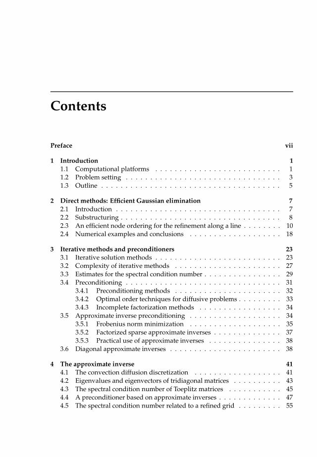
Contents
Preface vii
1 Introduction 1
1.1 Computational platforms . . . . . . . . . . . . . . . . . . . . . . . . . . 1
1.2 Problem setting . . . . . . . . . . . . . . . . . . . . . . . . . . . . . . . . 3
1.3 Outline . . . . . . . . . . . . . . . . . . . . . . . . . . . . . . . . . . . . . 5
2 Direct methods: Efficient Gaussian elimination 7
2.1 Introduction . . . . . . . . . . . . . . . . . . . . . . . . . . . . . . . . . . 7
2.2 Substructuring . . . . . . . . . . . . . . . . . . . . . . . . . . . . . . . . . 8
2.3 An efficient node ordering for the refinement along a line . . . . . . . . 10
2.4 Numerical examples and conclusions . . . . . . . . . . . . . . . . . . . 18
3 Iterative methods and preconditioners 23
3.1 Iterative solution methods . . . . . . . . . . . . . . . . . . . . . . . . . . 23
3.2 Complexity of iterative methods . . . . . . . . . . . . . . . . . . . . . . 27
3.3 Estimates for the spectral condition number . . . . . . . . . . . . . . . . 29
3.4 Preconditioning . . . . . . . . . . . . . . . . . . . . . . . . . . . . . . . . 31
3.4.1 Preconditioning methods . . . . . . . . . . . . . . . . . . . . . . 32
3.4.2 Optimal order techniques for diffusive problems . . . . . . . . . 33
3.4.3 Incomplete factorization methods . . . . . . . . . . . . . . . . . 34
3.5 Approximate inverse preconditioning . . . . . . . . . . . . . . . . . . . 34
3.5.1 Frobenius norm minimization . . . . . . . . . . . . . . . . . . . 35
3.5.2 Factorized sparse approximate inverses . . . . . . . . . . . . . . 37
3.5.3 Practical use of approximate inverses . . . . . . . . . . . . . . . 38
3.6 Diagonal approximate inverses . . . . . . . . . . . . . . . . . . . . . . . 38
4 The approximate inverse 41
4.1 The convection diffusion discretization . . . . . . . . . . . . . . . . . . 41
4.2 Eigenvalues and eigenvectors of tridiagonal matrices . . . . . . . . . . 43
4.3 The spectral condition number of Toeplitz matrices . . . . . . . . . . . 45
4.4 A preconditioner based on approximate inverses . . . . . . . . . . . . . 47
4.5 The spectral condition number related to a refined grid . . . . . . . . . 55

x Contents
5 Recursive solution methods 61
5.1 Decoupling in one dimension . . . . . . . . . . . . . . . . . . . . . . . . 61
5.2 A solver based on recursive decoupling . . . . . . . . . . . . . . . . . . 63
5.2.1 Description of the solver . . . . . . . . . . . . . . . . . . . . . . . 63
5.2.2 Complexity of the solver . . . . . . . . . . . . . . . . . . . . . . . 65
5.3 Decoupling in two dimensions . . . . . . . . . . . . . . . . . . . . . . . 66
5.4 Breakdown of uniform 2-D grids . . . . . . . . . . . . . . . . . . . . . . 71
5.5 Three algorithms based on forced repeated decoupling . . . . . . . . . 73
5.5.1 A recursive preconditioner: I . . . . . . . . . . . . . . . . . . . . 74
5.5.2 A recursive preconditioner: II . . . . . . . . . . . . . . . . . . . . 75
5.5.3 A recursive preconditioner: III . . . . . . . . . . . . . . . . . . . 76
5.6 Complexity of the algorithms . . . . . . . . . . . . . . . . . . . . . . . . 77
6 NumLab concepts 79
6.1 Introduction . . . . . . . . . . . . . . . . . . . . . . . . . . . . . . . . . . 79
6.2 The foundation of NumLab . . . . . . . . . . . . . . . . . . . . . . . . . 84
6.3 The NumLab elements . . . . . . . . . . . . . . . . . . . . . . . . . . . . 85
6.4 The NumLab operators . . . . . . . . . . . . . . . . . . . . . . . . . . . . 86
6.4.1 Systems of equations . . . . . . . . . . . . . . . . . . . . . . . . . 86
6.4.2 Solvers and Preconditioners . . . . . . . . . . . . . . . . . . . . . 87
6.4.3 Partial differential equations . . . . . . . . . . . . . . . . . . . . 89
6.4.4 Ordinary differential equations . . . . . . . . . . . . . . . . . . . 91
6.5 The NumLab factored out common components . . . . . . . . . . . . . 92
6.5.1 The Grid module . . . . . . . . . . . . . . . . . . . . . . . . . . . 92
6.5.2 The Space module . . . . . . . . . . . . . . . . . . . . . . . . . . 94
6.5.3 The Function module . . . . . . . . . . . . . . . . . . . . . . . 94
6.5.4 The Operator module . . . . . . . . . . . . . . . . . . . . . . . 95
6.5.5 The Solver module . . . . . . . . . . . . . . . . . . . . . . . . . 96
6.5.6 NumLab components . . . . . . . . . . . . . . . . . . . . . . . . 96
6.6 NumLab implementation . . . . . . . . . . . . . . . . . . . . . . . . . . 97
7 NumLab preconditioners 101
7.1 Introduction . . . . . . . . . . . . . . . . . . . . . . . . . . . . . . . . . . 101
7.2 Numerical results in one dimension . . . . . . . . . . . . . . . . . . . . 103
7.3 Numerical results in two dimensions . . . . . . . . . . . . . . . . . . . . 110
7.4 Numerical results in three dimensions . . . . . . . . . . . . . . . . . . . 116
8 Conclusions and future work 123
8.1 Conclusions . . . . . . . . . . . . . . . . . . . . . . . . . . . . . . . . . . 123
8.2 Directions for the future . . . . . . . . . . . . . . . . . . . . . . . . . . . 124
A Pentadiagonal Toeplitz matrices 127
Contents xi
B Turing completeness 129B.1 Alphabets and language . . . . . . . . . . . . . . . . . . . . . . . . . . . 129B.2 The Turing machine . . . . . . . . . . . . . . . . . . . . . . . . . . . . . . 129B.3 Primitive recursive functions . . . . . . . . . . . . . . . . . . . . . . . . 132B.4 µ-Recursive functions . . . . . . . . . . . . . . . . . . . . . . . . . . . . . 135
Bibliography 139
Index 147
Summary 149
Samenvatting 151
Curriculum Vitae 153


Chapter 1
Introduction
1.1 Computational platforms
The past few decades has witnessed a revolutionary increase in usage of computersystems in scientific research. As systems became more attractive with respect toprice and performance, simulations run on computer platforms became a good al-ternative to real experiments. Typical application areas are civil engineering, medicalsciences, hydrodynamics or aerodynamics.Modern computer applications can accurately model complex problems with largeamounts of parameters and variables, and generate large sets of computed data.These can have sizes of many gigabytes like in computational fluid dynamics sim-ulations, as e.g. are met in weather forecasts. Since the performance of computershas drastically improved, it has now become relatively easy to run simulations andproduce large datasets in a fairly short runtime.One important aspect of analyzing the produced datasets and acquiring insight inthe simulated problem is scientific visualization. A most common way is to plot thecomputed data, and examine this for further analysis. One step further is tracking,which gives more interaction with the simulation. At each (time) step of the simula-tion, the data produced is directly visualized, graphical or numerical, for inspection.This way the simulation can be monitored during runtime and the process can bestopped when the computed data is considered to be invalid. In order to avoid theseinvalid results, the whole process can be restarted after changing the input.However, though tracking is a nice feature to control the simulation in a more inter-active manner, this option is not sufficient when many input parameters are present.For example, when the simulation is to be run with different parameters it has tobe halted, reconfigured and restarted. Interactive steering is a means to control the(visualization and simulation) parameters interactively and to overcome the prob-lem of halting, reconfiguring and restarting. Parameters can be changed during thesimulation itself, and the visual and numerical tracking offers immediate feedback.
One of the biggest problems of early simulation applications was the monolithic andspecialized nature of the software. These applications were designed for a very re-stricted set of problems and did lack a certain amount of tracking and steering. Inprinciple input and output data was read and written to file for further analysis. This
2 Chapter 1: Introduction
approach to modeling and simulating is very uneconomical and inflexible and hasprompted the appearance of libraries for greater reusability of application softwareand application knowledge. However, a researcher is predominantly occupied withperforming research in an often very complex and specialized environment, oftenhaving no application software at hand. Moreover, the researcher does not have thetime to develop, implement and test a sophisticated software platform for the par-ticular research area, not to mention the possibility that the researcher does not havethe required programming skills. So, what is needed is a highly flexible, visual andeasy-to-use software platform and programming environment that allows a (inexpe-rienced) researcher to reuse existing components in an easy way to run simulations.On top of this the researcher should be able to extend the existing platform and en-vironment by newly developed simulation software for future use.
Building such custom tailored software by reusing existing components has beenconsidered at several places. The most successful solutions come in the form of vi-sual programming environments, such as AVS [97] or Iris Explorer [50]. But alsopackages that offer a whole range of specialized routines, such as Matlab [67] orMathematica [107], are sophisticated tools for scientific applications. For such plat-forms there are several aspects that are important. First of all there have to be com-ponents. These are the reusable building bricks from which new applications can bemade. Secondly there are control mechanisms that drive and steer the componentsthat are put together in an application. Thirdly, a data exchange model is used to com-municate and transfer between the various primitive units. Obviously, this modelshould be generic enough in order to communicate with non-platform software. Fi-nally a user interface should be available that offers the researcher the possibility totrack and steer the simulation.
In the future one may imagine that for an industrial problem, a computer will ”read“a mathematical model and discretization from a book or paper and construct a soft-ware application for all required calculations. In this thesis we make a step intothat direction. The software itself may have various representations, from classicalsource code line representation up to a modern interactive visual one. The latter rep-resentation facilitates rapid alterations and adaptations for research purposes andapplication development.
The need for such platforms is apparent for research groups who spend considerabletime on the development of application software. A first step toward such a platformwas made in [29, 61]; this platform was called Numlab. Numlab allowed a certainamount of flexibility as components of an application could be changed, and com-municated with existing mathematical packages such as Matlab and Mathematica.However, this version of Numlab was based on an inhouse developed interpreterlanguage which made the platform monolithic in some sense. One of the drawbackswas that this did not allow implementation of additional tools in an easy way. Itcan be compared to a library that needs to close down before a new book can beadded: The book has to be placed on the proper shelf and the inventory list must beupdated by hand. Then the library can reopen. In this thesis we present a concrete
Problem setting 3
and interactive visual workbench (Lab) for numerical computations (Num) and vi-sualization: NumLab. It contains an application called network editor ([93]) and anexisting C++ interpreter ([27]). Source code is created with a computer mouse andsimple clicks: The user selects components from libraries (called modules) and con-nects inputs and outputs. In NumLab a new book can be added without the need toclose down the library. The book is placed on the correct shelf and the inventory listis updated automatically.
1.2 Problem setting
Since NumLab is quite an ambitious project, we shall concentrate ourselves on aparticular problem from real life. Our goal is to extend NumLab in such a waythat we have all the necessary tools to tackle this problem. A typical problem ofwhat is to be solved using the NumLab workbench is that of the moisture and saltion transportation in a brick wall. The prediction of salt ion transport is important,because unbalanced salt concentrations damage bricks (see [11, 59, 62, 63, 80]).
0 0.05 0.1 0.15 0.2 0.25 0.3 0.35 0.4 0.45 0.52
3
4
5
6
7
8
9
10
11
moisture content u(x)
diffu
sion
coe
ffici
ent
D(u
)
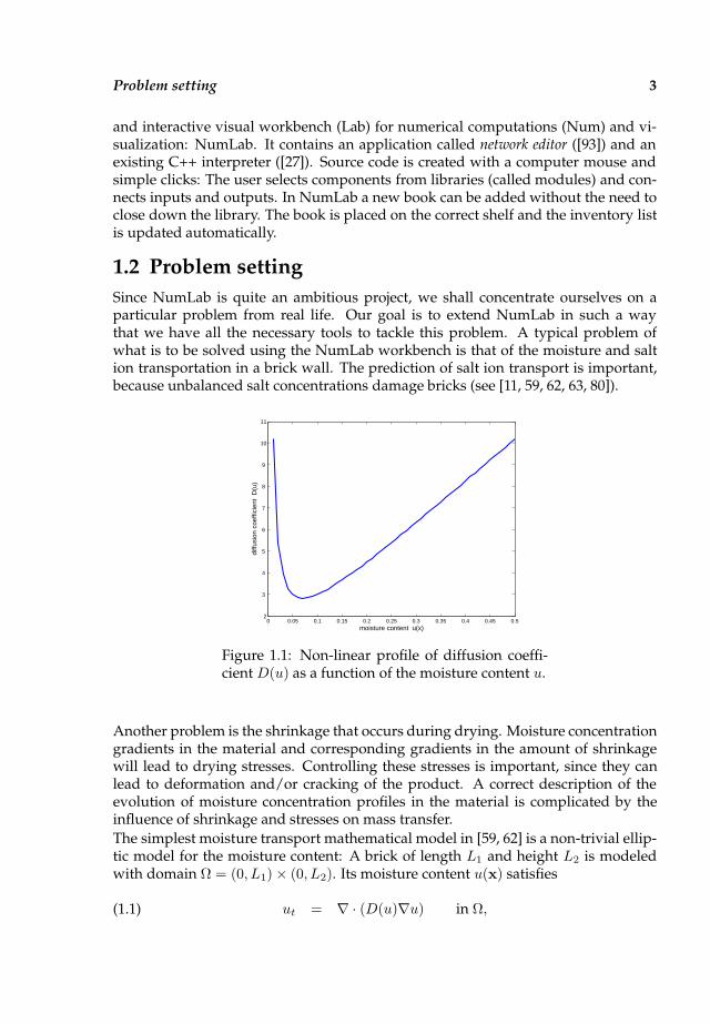
Figure 1.1: Non-linear profile of diffusion coeffi-cient D(u) as a function of the moisture content u.
Another problem is the shrinkage that occurs during drying. Moisture concentrationgradients in the material and corresponding gradients in the amount of shrinkagewill lead to drying stresses. Controlling these stresses is important, since they canlead to deformation and/or cracking of the product. A correct description of theevolution of moisture concentration profiles in the material is complicated by theinfluence of shrinkage and stresses on mass transfer.
The simplest moisture transport mathematical model in [59, 62] is a non-trivial ellip-tic model for the moisture content: A brick of length L1 and height L2 is modeledwith domain Ω = (0, L1) × (0, L2). Its moisture content u(x) satisfies
(1.1) ut = ∇ · (D(u)∇u) in Ω,

4 Chapter 1: Introduction
and u(x) satisfies some mixed boundary conditions on δΩ. The initial solution u0
has a transition layer at x1 = L1. The non-linearity of the diffusion coefficient isschematically represented in figure 1.1.Typically a problem like (1.1) is first discretized by a numerical method like the Fi-nite Element Method (FEM) or the Finite Difference Method (FDM). To this end oneneeds a grid, i.e., a set of points connected by lines which, e.g., give rise to elements(FEM) which together cover the domain. Because of the typical form of the PDE, weneed a much finer grid at the boundary of a ”brick“ than in the interior. In figure 1.2we have depicted two typical choices for such a mesh, embedded in a larger frameof more bricks. The (non-linear) equations describing the moisture content at thevarious nodes are then solved by e.g. Newton’s method. At the heart of this methodwe encounter a linear system that we can write in generic form as
(1.2) Ax = b.
Since the grid is not uniform such linear systems will be ill-conditioned in general.This hampers solving (1.2) efficiently.Rather than intending to solve a problem like (1.1), we consider the more genericlinear diffusion problem
(1.3)−∇ · a∇u+ cu = f in Ω = (0, 1)d ⊂ Rd,
u = g at ∂Ω.
The linear system arising from discretizing (1.3) may be ill-conditioned due to twosources. In general, a non-smooth source term f will result in a non-smooth solutionu of (1.3). In order to get an accurate solution, grids with local refinements as infigure 1.2 are required. A consequence of such refinements is that the resulting linearsystem, as in (1.2), is unbalanced because of the large differences in scale. In fact thisis similar to a very inhomogeneous grid due to a rapidly varying diffusion coefficienta. As remarked above, this means that the linear system becomes ill-conditioned.Another problem is that due to the relatively large number of gridpoints near theboundary the number of unknowns may rise enormously. Hence the problem size
Figure 1.2: A piece of wall with an unstructured and structured grid.

Outline 5
increases likewise which has its effects on efficient implementation and computation.Both phenomena, an ill-conditioned system and a large number of unknowns, leadto a larger computational complexity in general. In order to reduce this, techniquescalled preconditioning have been developed to reduce this complexity. However, forthe problem at hand no really efficient techniques exist.In this thesis we therefore will concentrate on constructing methods to solve linearsystems arising from configurations like the ones shown in figure 1.2. More in par-ticular, we focus on a typical brick with such a highly non-uniform mesh and willdevelop new ways to tackle the ill-conditioning and thus improve efficiency of it-erative solvers. This then will be the test to demonstrate our platform NumLab.The construction, outline and testing then constitutes the second major aspect of thisthesis.
1.3 Outline
As noted above we deal with two major subjects in this thesis. The first of theseis the NumLab workbench to facilitate numerical simulations. Secondly we extendNumLab by adding tools that are designed for solving the problem as described inthe previous section. Before we consider in detail the NumLab workbench, we mustfirst construct, discuss and analyse the tools we want to add.First in Chapter 2 a direct method is presented for the solution of convection domi-nated problems. In particular, we focus on grids that have refinement layers whichare reminiscent of the brick-wall configuration. For such refinements this chaptershows that a complete Gaussian factorization can be efficient with respect to both fill-in as well as the band-width if the degrees of freedom are numbered such that theyexploit the special grid structure. This efficient way to factorize the matrix meansthat inverses can be computed with an almost optimal number of floating pointsoperations (flops).Next, in Chapter 3, iterative methods are examined; these are usually more efficientthan Gaussian elimination considered before. The main idea of such iterative meth-ods is that the solution is computed by successive updating the existing approxi-mation. If the method is successful, the approximation is close enough to the exactsolution after a number of iterations, given a desired accuracy for the computed solu-tion. This process of iterating and constructing the solution is described for a varietyof iterative methods. Whereas with Gaussian factorization it is known beforehandthat the solution can be found after the successful factorization, which can be viewedas one iteration, for iterative methods it is not known a priori how many iterationsare required to obtain the solution. A priori knowledge of this is important, sincethe number of iterations determines the computational complexity. Unfortunately,an explicit formula for the minimum number of iterations needed is known for fewiterative methods only. Another important notion in iterative methods is the condi-tion number of the matrix. This condition number can be seen as a measure for the”quality“ of the matrix and is important for error estimates. We also look at methodsthat can improve the computational complexity of solving the problem. When solv-ing a problem by an iterative method, the computational complexity often growspolynomially with the number of unknowns. This is undesirable. Ideally the com-

6 Chapter 1: Introduction
putational complexity should be of the same order of magnitude as the number ofunknowns. In general terms, this means that every unknown has to be ”looked at“only once in order to obtain the solution. Thus, what we want is an efficient wayto improve this computational complexity. This is called preconditioning. What canbe judged from this term is that the original problem is adapted such that the newproblem is better conditioned. This in turn might lead to fewer iterations and hence alower computational complexity. However, not all types of problems are that simpleto precondition. In this chapter we address several methods that result in a theoreti-cally ideal computational complexity for a specific type of problems. As our problemof interest does not have such properties, we concentrate on a special class of pre-conditioning techniques which are based on approximated inverses (Section 3.5).In Chapter 4 we look into these types of techniques in more detail. Of particularinterest for this chapter is a slightly modified form of the preconditioner. For thisso-called modified approximate inverse, several results are obtained in this chapter.Numerical examples show that these also hold for the original unmodified versionwhich is used in computations.The approximate inverse related preconditioner is examined further in Chapter 5.Here it is shown that by applying this preconditioner, the resulting new problemcan be decoupled for one dimensional problems. This phenomenon gives rise toa recursive solution method by successive application of the approximate inverse.Unfortunately, in two dimensions this cannot be generalized straightforwardly. Wepoint at the properties that are inherited from the one dimensional case, and whichare not. This leads to a different solution procedure and we provide suggestions forutilizing approximate inverse in two dimensions in a recursive manner.The remainder of this thesis is devoted to the construction and use of NumLab. Tostart with, in Chapter 6 we discuss the basic ideas of our platform. NumLab enablesus to implement and test new ideas by reusing existing components and buildingnew components easily either from scratch or by putting together existing compo-nents. In NumLab, mathematical concepts, like operators and solvers, are imple-mented using a uniform interface with a generic formulation. This enables one tochange components and parameters in a simulation. Also complex numerical toolsto solve complex problems can be composed with just a few components. Finally, alltools can be used for visual programming which gives the researcher an overview ofthe simulation and direct ways to interact with the simulation.In Chapter 7 we continue with the NumLab workbench, and examine how we canimplement the new tools presented in Chapter 4. This chapter is the synthesis ofour computational platform (NumLab) in which (complex) mathematical tools (theapproximate inverse preconditioner) can be utilized in an easy manner. We seize theopportunity to present several numerical examples to show the effectiveness of thepreconditioner from Chapter 4 for certain types of problems. In NumLab, runninganother example can be obtained by simply changing a parameter in the requiredmodule. This is detailed as well.Finally, Chapter 8 summarizes the most important conclusions of this thesis. Fur-thermore some recommendations for future work are addressed.
Chapter 2
Direct methods: Efficient Gaussianelimination
In this chapter we discuss an efficient implementation of Gaussian elimination, suitedfor the solution of convection dominated problems. The domains of interest are suchthat they can be divided into similar substructures. Brick walls as have been dis-cussed in Section 1.2 are a good example of such domains. The layer between twosubstructures (two bricks for example) may be such that local refinement is neededto capture the solution accurately. This part of a brick wall is simplified, but the char-acteristics of uniform coarse parts with refinement layers in between are inherited.For such locally refined grids we present a numbering of the degrees of freedomwith favourable properties. When k levels of refinement are used the amount of fill-in is O(k2k). The original number of degrees of freedom n is O(2k), which impliesthat the complexity of the method is O(n logn). This fill-in is comparable to the fill-in-optimized minimum degree algorithm [46, 95]. The band-width is comparable tothe band-width-optimizing reverse Cuthill-McKee ordering [45]. Another benefit isthat Gaussian elimination is not only applicable to Poisson type problems, but alsoto convection diffusion problems.
2.1 Introduction
The local bisection refinement, see [70], best preserves the regular substructures ofthe domain of interest, much better than the more common Delaunay type gridding(see [56]). Both grids in figure 1.2 – left Delaunay, right bisection – are obtained usingthe same input data. The bisection refinement preserves the substructures best, andin fact leads to semi-regular grids.
An even more important reason to use grids created by bisection refinement is thatsemi-regular grids can also also be obtained in three and more dimensions, as wellas that efficient storage scheme and optimal order preconditioners exist for such re-finement along lines, see [66].
Several efficient solvers have been published for elliptic problems that are discretizedwith finite elements on refined grids. For instance, the optimal AMLI [7, 8], andoptimal BPX [24]. In principle, these solvers can solve elliptic problems withoutdomain decomposition. When convection dominates, the solvers no longer appear
8 Chapter 2: Direct methods: Efficient Gaussian elimination
to be efficient.
In this chapter we are interested in the subdomains which contain a line along whichall mesh refinement is situated (see figure 2.1). For this special subdomain, we showthat a Gaussian elimination can be performed such that a near optimal band-widthand near optimal fill-in is achieved. The results are based on a proper numberingof the degrees of freedom. The minimum degree algorithm [46] has somewhat lessfill-in, even though no optimal tie-breaking strategy is known when different degreesof freedom have the same connectivity. It should be noted that the total amount offill-in is quite sensitive to the tie-breaking strategy.
When solving the linear system of equations, our exact factors can be replaced byan incomplete version (see for instance [58, 74, 39, 78]), combined with Krylov-spacebased iterative solvers [86, 102]. However, because the focus of this chapter is ondemonstrating that we get optimal fill-in and band width matrix factors for the fullGaussian elimination process, we do not provide an analysis of the incomplete case.
The substructures of interest are introduced in Section 2.2. In Section 2.3 a number-ing of degrees of freedom is presented for which Gaussian elimination leads to anamount of fill-in close to that of the fill-in-optimized minimum degree algorithm [46],and on top leads to a band-width which is close to that of the reverse Cuthill-McKeeordering [45]. In the final section some examples are given to illustrate the new num-bering scheme.
2.2 Substructuring
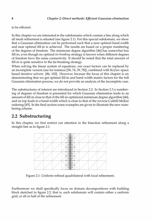
In this chapter, we first restrict our attention to the bisection refinement along astraight line as in figure 2.1.
Figure 2.1: Uniform refined quadrilateral with local refinement.
Furthermore we shall specifically focus on domain decompositions with buildingblock sketched in figure 2.2, that is, each subdomain will contain either a uniformgrid, or all or half of the refinement.

Substructuring 9
1 x 1 1 x 8 8 x 8
Figure 2.2: Grids which capture different levels of detail (1x1, 1x8 and 8x8).
The subdomains we examine in detail contain all refinement and are concentratedaround the refinement along a straight line. For these subdomains, we denote theamount of horizontal blocks (layers) by K, and k denotes the level of refinement.The related grids are called GK,k .
Figure 2.3: Refined grids GK,k forK = 4, k = 1, 2.
Figure 2.4: Refined grids GK,k forK = 8, k = 1, 2.
Let k ≥ 1. Each horizontal block is obtained by applying 2(k − 1) levels of bisectionrefinement. Its connectivity-graph is called Bk. (Each two subsequent refinementsshrink the smallest edge-length by a factor two.) Figure 2.3 and figure 2.4 show therefined grids related to K = 4 and K = 8 for both k = 1 and k = 2. Let Bk denotethe connectivity graph associated to a horizontal block. With Bk, we associate thecoarse grid element-size H = 1/K and smallest element-size h = H · 2−k. Theseconnectivity graphs Bk are discussed in more detail in the next section.
10 Chapter 2: Direct methods: Efficient Gaussian elimination
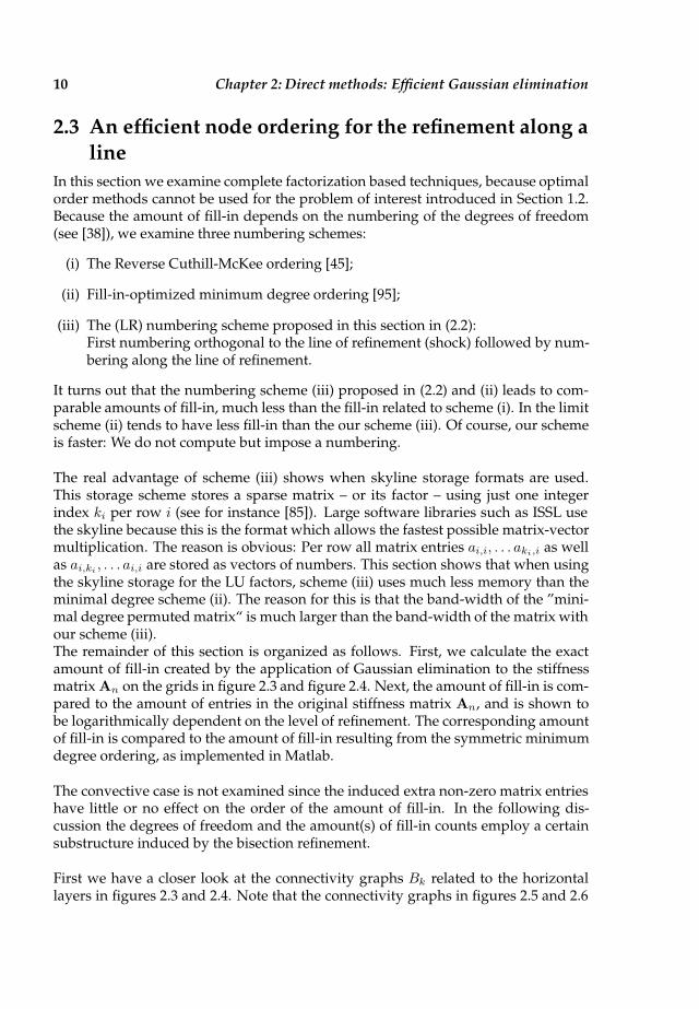
2.3 An efficient node ordering for the refinement along a
line
In this section we examine complete factorization based techniques, because optimalorder methods cannot be used for the problem of interest introduced in Section 1.2.Because the amount of fill-in depends on the numbering of the degrees of freedom(see [38]), we examine three numbering schemes:
(i) The Reverse Cuthill-McKee ordering [45];
(ii) Fill-in-optimized minimum degree ordering [95];
(iii) The (LR) numbering scheme proposed in this section in (2.2):First numbering orthogonal to the line of refinement (shock) followed by num-bering along the line of refinement.
It turns out that the numbering scheme (iii) proposed in (2.2) and (ii) leads to com-parable amounts of fill-in, much less than the fill-in related to scheme (i). In the limitscheme (ii) tends to have less fill-in than the our scheme (iii). Of course, our schemeis faster: We do not compute but impose a numbering.
The real advantage of scheme (iii) shows when skyline storage formats are used.This storage scheme stores a sparse matrix – or its factor – using just one integerindex ki per row i (see for instance [85]). Large software libraries such as ISSL usethe skyline because this is the format which allows the fastest possible matrix-vectormultiplication. The reason is obvious: Per row all matrix entries ai,i, . . . aki,i as wellas ai,ki , . . . ai,i are stored as vectors of numbers. This section shows that when usingthe skyline storage for the LU factors, scheme (iii) uses much less memory than theminimal degree scheme (ii). The reason for this is that the band-width of the ”mini-mal degree permuted matrix“ is much larger than the band-width of the matrix withour scheme (iii).The remainder of this section is organized as follows. First, we calculate the exactamount of fill-in created by the application of Gaussian elimination to the stiffnessmatrix An on the grids in figure 2.3 and figure 2.4. Next, the amount of fill-in is com-pared to the amount of entries in the original stiffness matrix An, and is shown tobe logarithmically dependent on the level of refinement. The corresponding amountof fill-in is compared to the amount of fill-in resulting from the symmetric minimumdegree ordering, as implemented in Matlab.
The convective case is not examined since the induced extra non-zero matrix entrieshave little or no effect on the order of the amount of fill-in. In the following dis-cussion the degrees of freedom and the amount(s) of fill-in counts employ a certainsubstructure induced by the bisection refinement.
First we have a closer look at the connectivity graphs Bk related to the horizontallayers in figures 2.3 and 2.4. Note that the connectivity graphs in figures 2.5 and 2.6
An efficient node ordering for the refinement along a line 11
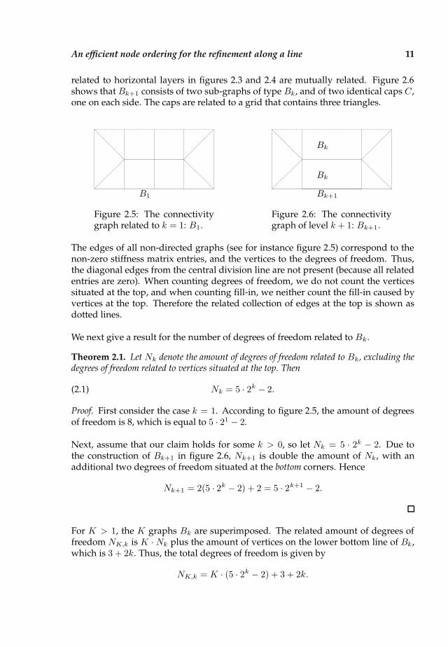
related to horizontal layers in figures 2.3 and 2.4 are mutually related. Figure 2.6shows that Bk+1 consists of two sub-graphs of type Bk, and of two identical caps C,one on each side. The caps are related to a grid that contains three triangles.
PSfrag replacements
B1
Figure 2.5: The connectivitygraph related to k = 1: B1.
PSfrag replacementsBk
Bk
Bk+1
Figure 2.6: The connectivitygraph of level k + 1: Bk+1.
The edges of all non-directed graphs (see for instance figure 2.5) correspond to thenon-zero stiffness matrix entries, and the vertices to the degrees of freedom. Thus,the diagonal edges from the central division line are not present (because all relatedentries are zero). When counting degrees of freedom, we do not count the verticessituated at the top, and when counting fill-in, we neither count the fill-in caused byvertices at the top. Therefore the related collection of edges at the top is shown asdotted lines.
We next give a result for the number of degrees of freedom related to Bk.
Theorem 2.1. Let Nk denote the amount of degrees of freedom related to Bk, excluding thedegrees of freedom related to vertices situated at the top. Then
(2.1) Nk = 5 · 2k − 2.
Proof. First consider the case k = 1. According to figure 2.5, the amount of degreesof freedom is 8, which is equal to 5 · 21 − 2.
Next, assume that our claim holds for some k > 0, so let Nk = 5 · 2k − 2. Due tothe construction of Bk+1 in figure 2.6, Nk+1 is double the amount of Nk, with anadditional two degrees of freedom situated at the bottom corners. Hence
Nk+1 = 2(5 · 2k − 2) + 2 = 5 · 2k+1 − 2.
For K > 1, the K graphs Bk are superimposed. The related amount of degrees offreedom NK,k is K ·Nk plus the amount of vertices on the lower bottom line of Bk,which is 3 + 2k. Thus, the total degrees of freedom is given by
NK,k = K · (5 · 2k − 2) + 3 + 2k.
12 Chapter 2: Direct methods: Efficient Gaussian elimination
Note that we pretend not to eliminate the vertices at the Dirichlet boundaries (topand bottom). The elimination would make the fill-in count below even more elabo-rate, but has little effect on the amount of fill-in. Thus, as a matter of fact, we countthe fill-in of a stiffness matrix An induced by Neumann boundary conditions on thedomain’s top and bottom.
The Gaussian elimination process applied to An leads to the standard upper andlower triangular factors such that An = LnUn. We count the amount of potentialnon-zero entries ρ in Un, excluding its diagonal. The actual amount of fill-in followsfrom ρ and the amount of non-zero entries in An. Because the grid depends on Kand k, so do An and ρ; we shall use the notation AK,k and ρK,k respectively whennecessary.
The amount of entries ρ depends on the numbering of the degrees of freedom (num-bering of the vertices of the graphs Bk). We distinguish the following numberingschemes:
(2.2)(LR) First from left to right, next from bottom to top;(BT ) First from bottom to top, next from left to right.
The (LR) scheme is the one which leads to a nearly optimal band-width combinedwith nearly optimal fill-in. The (BT) scheme performs poorly with respect to bothfill-in and band-width. The main reason that the (LR) numbering performs so wellturns out to be that the degrees of freedom are numbered first in a direction orthogonal tothe resolved line, and next in the direction tangent to this line. This numbering schemeshortens possible paths which can lead to the creation of fill-in.
In [45] paths have been characterized that can cause fill-in. Let i < k be the numbersof two degrees of freedom. A related (potential) non-zero fill-in is created in UK,k
during Gaussian elimination if there is a fill-in path: A path from vertex vi to vertexvk through vertices v0, . . . , vi−1 ([76, Th. 3.3]). All counts for ρ depend on the (LR)numbering. When graph Bk is related to a middle layer of a grid GK,k , its fill-inpaths can leave and reenter through its bottom horizontal line. Such paths are calledreentrant paths, all other paths are called non-reentrant, or internal.
Definition 2.2. For k > 0, define
(i) Pk, the amount of non-top vertices induced fill-in paths (inc. reentrant) of Bk;
(ii) Tk, the amount of top vertices induced fill-in paths of Bk;
(iii) Rk, the amount of bottom vertices reentrant fill-in paths of Bk.
Then the amount of non-zero entries ρK,k is given by
(2.3) ρK,k = K · Pk + Tk −Rk.
In Theorem 2.3 below where an explicit expression for ρK,k for the (LR) scheme isgiven, several types of fill-in paths are distinguished:

An efficient node ordering for the refinement along a line 13
• To the right, or diagonally or vertically up (also non-zero entry in An);
• To the left, and next diagonally or vertically up;
• If possible, first down from vi, next left, and finally up to a vertex on a horizon-tal line above vi;
• If possible, first down from vi, next right, and finally up to a vertex on a hori-zontal line above or containing vi.
Theorem 2.3. Let AK,k be the standard stiffness matrix obtained on the grids GK,k infigures 2.3 – 2.4, using an (LR) numbering scheme. Assume that AK,k = LK,kUK,k is fac-tored by Gaussian elimination. Then the amount of potential non-zero entries in the strictlyupper triangular part of UK,k is
(2.4) ρK,k = K ·(
(10k + 16) · 2k − 4k − 7)
+ 2(1 + k).
Proof. The refined grid consists of K horizontal layers, each related to a graph Bk.From (2.3) it follows that we have to count all of (i) Pk, (ii) Tk and (iii) Rk.
First, consider case (i). To determine Pk, we first count the non-zero entries relatedto the bottom corner vertices of Bk. This amount equals
(2.5) 4k + 7.
The proof now employs induction with respect to the level k. Note that fill-in pathscounted for Pk can be reentrant.For k = 1, the left corner vertex vlk has 6 fill-in paths ending at higher numberedvertices, and the right corner vertex vrk has 5 such paths, two of which are depictedin figure 2.7.
PSfrag replacementsB1
Figure 2.7: One fill-in path from vl1, and one fromvr1 .
14 Chapter 2: Direct methods: Efficient Gaussian elimination
Thus, for k = 1, the total amount of fill-in paths is:
6 + 5 = 4 · 1 + 7
Next, assume that (2.5) holds for some k ≥ 1. According to figure 2.6, Bk+1 has twosubgraphs of type Bk, and two cap graphs C, each introducing a new lower cornervertex vlk+1 and vrk+1. Now vlk+1 has a fill-in path to all vertices vlk,and vrk+1 has afill-in path to all vertices vrk.Each has two additional fill-in-paths with the two newtop left and right vertices of graph Bk+1. So the new bottom left and right cornervertices have a total of
4k + 7 + 2 + 2 = 4(k + 1) + 7
fill-in paths.
For case (i), we next assert that:
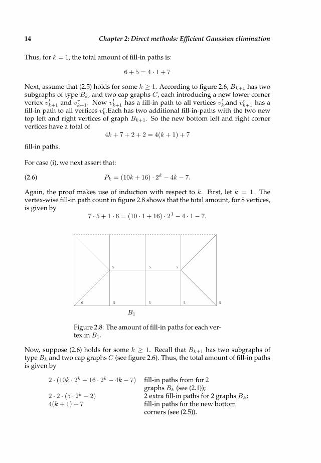
(2.6) Pk = (10k + 16) · 2k − 4k − 7.
Again, the proof makes use of induction with respect to k. First, let k = 1. Thevertex-wise fill-in path count in figure 2.8 shows that the total amount, for 8 vertices,is given by
7 · 5 + 1 · 6 = (10 · 1 + 16) · 21 − 4 · 1 − 7.
5
5 5 5
6 5 5 5PSfrag replacements
B1
Figure 2.8: The amount of fill-in paths for each ver-tex in B1.
Now, suppose (2.6) holds for some k ≥ 1. Recall that Bk+1 has two subgraphs oftype Bk and two cap graphs C (see figure 2.6). Thus, the total amount of fill-in pathsis given by
2 · (10k · 2k + 16 · 2k − 4k − 7) fill-in paths from for 2graphs Bk (see (2.1));
2 · 2 · (5 · 2k − 2) 2 extra fill-in paths for 2 graphs Bk;4(k + 1) + 7 fill-in paths for the new bottom
corners (see (2.5)).
An efficient node ordering for the refinement along a line 15
As desired, this adds up to (10(k + 1) + 16) · 2k+1 − 4(k + 1) − 7.
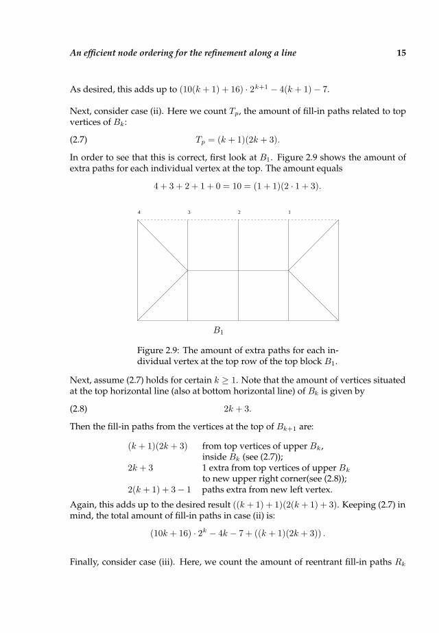
Next, consider case (ii). Here we count Tp, the amount of fill-in paths related to topvertices of Bk:
(2.7) Tp = (k + 1)(2k + 3).
In order to see that this is correct, first look at B1. Figure 2.9 shows the amount ofextra paths for each individual vertex at the top. The amount equals
4 + 3 + 2 + 1 + 0 = 10 = (1 + 1)(2 · 1 + 3).
4 3 2 1
PSfrag replacements
B1
Figure 2.9: The amount of extra paths for each in-dividual vertex at the top row of the top block B1.
Next, assume (2.7) holds for certain k ≥ 1. Note that the amount of vertices situatedat the top horizontal line (also at bottom horizontal line) of Bk is given by
(2.8) 2k + 3.
Then the fill-in paths from the vertices at the top of Bk+1 are:
(k + 1)(2k + 3) from top vertices of upper Bk,inside Bk (see (2.7));
2k + 3 1 extra from top vertices of upper Bkto new upper right corner(see (2.8));
2(k + 1) + 3 − 1 paths extra from new left vertex.
Again, this adds up to the desired result ((k + 1) + 1)(2(k + 1) + 3). Keeping (2.7) inmind, the total amount of fill-in paths in case (ii) is:
(10k + 16) · 2k − 4k − 7 + ((k + 1)(2k + 3)) .
Finally, consider case (iii). Here, we count the amount of reentrant fill-in paths Rk

16 Chapter 2: Direct methods: Efficient Gaussian elimination
related to bottom vertices of graphBk. To this end, we first count the total amount ofpaths related to bottom vertices, and next count and subtract the amount of internalpaths.
The total amount of fill-in paths related to bottom vertices of Bk is given by
(2.9) 4k2 + 13k + 9.
For k = 1, this holds, counting all such paths in figure 2.5. Assume this amount iscorrect for certain k ≥ 1. Then for k + 1 we have
4k2 + 13k + 9 for each bottom vertex in bottom Bk (see 2.9);2 · (2k + 3) 2 extra for each bottom vertex in bottom Bk (see (2.8));4(k + 1) + 7 extra from two new vertices C graphs.
The total amount now is 4(k + 1)2 + 13(k + 1) + 9 indeed.Next we count the amount of internal paths
(2.10) 2k2 + 10k + 8.
For k = 1, this holds (see figure 2.5). Assume this amount is correct for certain k ≥ 1.Then for k + 1:
2k2 + 10k + 8 for each bottom vertex in bottom Bk (see 2.10);2k + 3 − 1 1 extra for each bottom vertex in bottom Bk,
except right corner (see (2.8));2 2 extra for right bottom corner vertex in Bk;2 for the new left bottom corner vertex (in C graph);2k + 3 + 2 for the new right bottom corner vertex (in C graph).
From (2.10) and (2.9) we obtain thus
Rk = (4k2 + 13k + 9) − (2k2 + 10k + 8) = 2k2 + 3k + 1.
Finally, note that
Tk −Rk = (k + 1)(2k + 3) − (2k2 + 3k + 1) = 2(1 + k),
which shows that (2.4) holds.
Remark 2.4. Theorem 2.3 shows that the amount of entries in the factors of An isO(k · 2k). The amount of entries in An depends in a different manner on k:
Theorem 2.5. Let AK,k be the standard stiffness matrix obtained on the grids GK,k infigures 2.3 – 2.4. Then the amount of non-zero entries in AK,k is given by
(2.11) AK,k = 25 · 2k−1 − 7.
An efficient node ordering for the refinement along a line 17
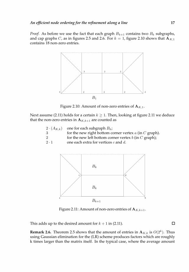
Proof. As before we use the fact that each graph Bk+1 contains two Bk subgraphs,and cap graphs C, as in figures 2.5 and 2.6. For k = 1, figure 2.10 shows that AK,1
contains 18 non-zero entries.
3 2 2
3 2 2 2 2PSfrag replacements
B1
Figure 2.10: Amount of non-zero entries of AK,1.
Next assume (2.11) holds for a certain k ≥ 1. Then, looking at figure 2.11 we deducethat the non-zero entries in AK,k+1 are counted as
2 · (AK,k) one for each subgraph Bk;3 for the new right bottom corner vertex a (in C graph).2 for the new left bottom corner vertex b (in C graph);2 · 1 one each extra for vertices c and d.
a b
c d
PSfrag replacementsBk
Bk
Bk+1
Figure 2.11: Amount of non-zero entries of AK,k+1.
This adds up to the desired amount for k + 1 in (2.11).
Remark 2.6. Theorem 2.5 shows that the amount of entries in AK,k is O(2k). Thususing Gaussian elimination for the (LR) scheme produces factors which are roughlyk times larger than the matrix itself. In the typical case, where the average amount
18 Chapter 2: Direct methods: Efficient Gaussian elimination
of entries per row of A is small, a factor k = 10 or k = 20 is a reasonable fill-in. Infact it can compensate for k = 10 or k = 20 iterations, had an iterative method beenused to solve Ax = b. Note that k = 20 corresponds to a difference in scales of 10−6.
2.4 Numerical examples and conclusions
In this last section we give two examples in order to illustrate the (LR) node num-bering scheme discussed in Section 2.3, and compare its efficiency to the reverseCuthill-McKee and minimum degree ordering schemes.
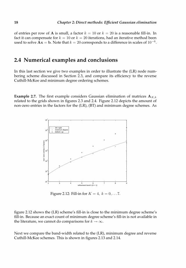
Example 2.7. The first example considers Gaussian elimination of matrices AK,k
related to the grids shown in figures 2.3 and 2.4. Figure 2.12 depicts the amount ofnon-zero entries in the factors for the (LR), (BT) and minimum degree schemes. As
2 3 4 5 6 7 8 910
1
102
103
104
105
106
107
refinement level k (K = 1)
non−
zero
ent
ries
in fa
ctor
s
left−right minimum degreebottom−up
Figure 2.12: Fill-in for K = 4, k = 0, . . . 7.
figure 2.12 shows the (LR) scheme’s fill-in is close to the minimum degree scheme’sfill-in. Because an exact count of minimum degree scheme’s fill-in is not available inthe literature, we cannot do comparisons for k → ∞.
Next we compare the band-width related to the (LR), minimum degree and reverseCuthill-McKee schemes. This is shown in figures 2.13 and 2.14.

Numerical examples and conclusions 19
0 10 20 30 40 50 60 70 80
0
10
20
30
40
50
60
70
80
nz = 887
(a) Left-right ordering
0 10 20 30 40 50 60 70 80
0
10
20
30
40
50
60
70
80
nz = 821
(b) Minimum degree or-dering
0 10 20 30 40 50 60 70 80
0
10
20
30
40
50
60
70
80
nz = 1201
(c) Rev. Cuthill-McKeeordering
Figure 2.13: Factors for the three ordering schemes (K, k) = (4, 2).
0 200 400 600 800 1000 1200
0
200
400
600
800
1000
1200
nz = 36007
(a) Left-right ordering
0 200 400 600 800 1000 1200
0
200
400
600
800
1000
1200
nz = 26639
(b) Minimum degree or-dering
0 200 400 600 800 1000 1200
0
200
400
600
800
1000
1200
nz = 284295
(c) Rev. Cuthill-McKeeordering
Figure 2.14: Factors for the three ordering schemes (K, k) = (4, 6).
As will be clear from these figures, the envelope of the factors of the reordered min-imum degree matrix is almost maximal, i.e. almost identical to the total amount ofdegrees of freedom. Thus, using a minimum degree ordering, matrix-vector imple-mentations for L and U should make use of column indexing. The L and U factorsfrom the (LR) scheme do not require such an indexing, whence matrix-vector mul-tiplication is likely to be faster. Furthermore, the band-width related to the (LR)scheme is comparable to the band-width optimizing reverse Cuthill-McKee scheme.

20 Chapter 2: Direct methods: Efficient Gaussian elimination
Figure 2.15: A brick covered by a lo-cally refined finite element grid.
Example 2.8. In this example we examine a brick-like structure as in figure 2.15, andin particular we look at the refinement layer near the boundary. This is the type ofgrid we had in mind in Section 1.2 as representation of a typical brick with a highlynon-uniform mesh toward the boundary. The initial uniform grid in these tests hassize 19× 19, and at each refinement step one level of bisection refinement is appliedto the layer of elements closest to the boundary. Figure 2.16 shows in detail this layerof interest, with several refinement steps.
Initial grid,
Figure 2.16: Initial uniform grid, the refinement layer at the bound-ary and three bisection steps.
First we compare the band-width related to the (LR), minimum degree and reverseCuthill-McKee ordering schemes. Results are shown in figures 2.17 and 2.18.
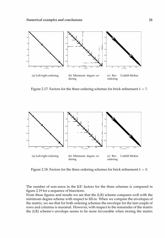
Numerical examples and conclusions 21
0 200 400 600 800 1000
0
200
400
600
800
1000
nz = 21004
(a) Left-right ordering
0 200 400 600 800 1000
0
200
400
600
800
1000
nz = 16654
(b) Minimum degree or-dering
0 200 400 600 800 1000
0
200
400
600
800
1000
nz = 43738
(c) Rev. Cuthill-McKeeordering
Figure 2.17: Factors for the three ordering schemes for brick refinement k = 7.
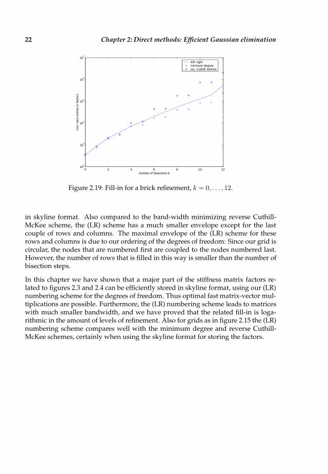
0 500 1000 1500 2000
0
500
1000
1500
2000
nz = 53790
(a) Left-right ordering
0 500 1000 1500 2000
0
500
1000
1500
2000
nz = 40538
(b) Minimum degree or-dering
0 500 1000 1500 2000
0
500
1000
1500
2000
nz = 181414
(c) Rev. Cuthill-McKeeordering
Figure 2.18: Factors for the three ordering schemes for brick refinement k = 9.
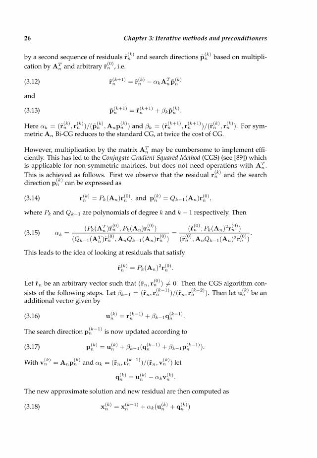
The number of non-zeros in the LU factors for the three schemes is compared infigure 2.19 for a sequence of bisections.From these figures and results we see that the (LR) scheme compares well with theminimum degree scheme with respect to fill-in. When we compare the envelopes ofthe matrix, we see that for both ordering schemes the envelope for the last couple ofrows and columns is maximal. However, with respect to the remainder of the matrixthe (LR) scheme’s envelope seems to be more favourable when storing the matrix
22 Chapter 2: Direct methods: Efficient Gaussian elimination
0 2 4 6 8 10 1210
2
103
104
105
106
107
number of bisections k
non−
zero
ent
ries
in fa
ctor
s
left−rightminimum degreerev. Cuthill−McKee
Figure 2.19: Fill-in for a brick refinement, k = 0, . . . , 12.
in skyline format. Also compared to the band-width minimizing reverse Cuthill-McKee scheme, the (LR) scheme has a much smaller envelope except for the lastcouple of rows and columns. The maximal envelope of the (LR) scheme for theserows and columns is due to our ordering of the degrees of freedom: Since our grid iscircular, the nodes that are numbered first are coupled to the nodes numbered last.However, the number of rows that is filled in this way is smaller than the number ofbisection steps.
In this chapter we have shown that a major part of the stiffness matrix factors re-lated to figures 2.3 and 2.4 can be efficiently stored in skyline format, using our (LR)numbering scheme for the degrees of freedom. Thus optimal fast matrix-vector mul-tiplications are possible. Furthermore, the (LR) numbering scheme leads to matriceswith much smaller bandwidth, and we have proved that the related fill-in is loga-rithmic in the amount of levels of refinement. Also for grids as in figure 2.15 the (LR)numbering scheme compares well with the minimum degree and reverse Cuthill-McKee schemes, certainly when using the skyline format for storing the factors.

Chapter 3
Iterative methods and preconditioners
In this chapter we address the problem of computing the solution of a linear sys-tem of equations resulting from the discretization of a convection diffusion equation.There are two main classes of algorithms to compute the solution of a linear system:direct methods and iterative methods. The Gaussian elimination technique discussedin Chapter 2 is an example of a direct method. In this chapter we focus on iterativemethods. We start with introducing the underlying problem and indicate some iter-ative methods. In particular we discuss the complexity of such methods and point atthe important factors determining this complexity. Methods to reduce this complex-ity are dealt with next. This includes approximate inverse techniques as they will bethe methods of choice in Chapter 4.
3.1 Iterative solution methods
In this thesis we will exclusively study linear systems of equations arising from theconvection diffusion equation
(3.1)−a∆u+ b · ∇u+ cu = f in Ω = (0, 1)d ⊂ Rd,
u = g at ∂Ω.
After discretization we typically obtain an n× n linear system of equations
(3.2) Anxn = bn.
For the following discussion the actual type of equation and discretization methodas such is not of importance. In contrast to Chapter 2 we will discuss iterative
methods to solve an equation like (3.2) here. Let x(0)n denote an initial guess and
r(0)n := bn − Anx
(0)n the residual. Then the sequence x
(k)n , k = 1, 2, . . . denotes the
iterates computed during the iterative process, with residuals r(k)n := bn − Anx
(k)n .
Finally, let e(k)n := x
(k)n − xn be the error at iteration step k.
Iterative solvers are classified as stationary or nonstationary. Stationary methods arebased on a splitting of the matrix An, denoted as
An = Pn −Qn,

24 Chapter 3: Iterative methods and preconditioners
where Pn is non-singular. For such methods the iteration can be expressed in thesimplified form
(3.3) Pnx(k+1)n = Qnx
(k)n + bn,
orx(k+1)n = P−1
n Qnx(k)n + P−1
n bn.
Now it is easy to see that for the error we have
e(k)n = (P−1
n Qn)ke(0)n .
As an example of stationary iterative methods consider the Successive Over RelaxationMethod (SOR). Here An is split up as An = Dn−Ln−Un where Dn, −Ln and −Un
denote the diagonal, lower-triangular and upper-triangular parts of An respectively,and let ω > 0. For the SOR method we take Pn = 1
ωDn−Ln and Qn = 1−ωω Dn+Un.
The parameter ω is called the relaxation parameter. Then the SOR iterative methodcan be written as
(3.4) x(k+1)n = (Dn − ωLn)−1(ωUn + (1 − ω)Dn)x(k)
n + ω(Dn − ωLn)−1bn.
For the iteration matrix we have
(3.5) P−1n Qn = (Dn − ωLn)
−1(ωUn + (1 − ω)Dn).
The value of ω is important for the convergence of the algorithm. Let ρ denote thespectral radius of the Jacobi matrix J(An) := D−1
n (Ln +Un), i.e. ρ = maxλ∈σ(J(An)) |λ|where σ(J(An)) is the spectrum of J(An). Then the theoretically optimal value forω is given by (cf. [9])
ωopt =2
1 +√
1 − ρ2.
There exists a host of such stationary methods; however they are not of much impor-tance for our particular problem here. We are actually more interested in nonstation-ary iterative methods. Though these are usually more difficult to implement, theycan be very effective. The difference between stationary and nonstationary methodsis that in nonstationary methods the computations involve information that changesat each iteration. The principle of these methods is that a projection process is em-
ployed one way or another. As such, at each iteration k the new residual r(k)n is
computed such that it is orthogonal to a subspace Kk of dimension k formed in thek − 1 previous iterations. In other words, we construct a new approximate solution
x(k)n such that
bn −Anx(k)n ⊥ Kk.
Of particular interest are subspaces Kk defined by
(3.6) Kk = spanr(0)n ,Anr
(0)n , . . . ,Ak−1
n r(0)n .

Iterative solution methods 25
This is the so called Ritz-Galerkin approach. Subspaces defined this way are calledKrylov subspaces, and methods based on orthogonalisation of the new residual overthe current subspace are called Krylov subspace methods. It should be noted that othermethods can be constructed by selecting other subspaces for the orthogonality con-dition.
The best known of these Krylov subspace methods is the Conjugate Gradient Method(CG) (see [51]) for symmetric positive definite systems. This method generates asequence of vectors that satisfy the Ritz-Galerkin condition in (3.6). In short, the CG
algorithm can be described as follows (see for example [9, 84]). Let p(k)n be the search
direction vector at iteration step k. Then the iterate x(k)n is updated as
(3.7) x(k+1)n = x(k)
n + αkp(k)n
for a scalar αk. Then for the new residual r(k+1)n
(3.8) r(k+1)n = r(k)
n − αkAnp(k)n .
With αk = (r(k)n , r
(k)n )/(p
(k)n ,Anp
(k)n ) we minimize the error (r
(k+1)n ,A−1
n r(k+1)n ) over
the existing subspace Kk. Finally the search direction is updated as well
(3.9) p(k+1)n = r(k+1)
n + βkp(k)n ,
with βk = (r(k+1)n , r
(k+1)n )/(r
(k)n , r
(k)n ). This ensures that r
(k+1)n and r
(k)n are orthogo-
nal.
For convergence estimates of the CG method the spectral condition number κ2 of An
is used. For a symmetric positive definite matrix An, if λn and λ1 are the maximumand minimum eigenvalues of An respectively, then
(3.10) κ2(An) =λnλ1.
Then it can be shown that after k iterations the error e(k)n satisfies
(3.11) ‖e(k)n ‖An ≤ 2
(
√
κ2(An) − 1√
κ2(An) + 1
)k
‖e(0)n ‖An ,
where ‖yn‖An := (yn,Anyn)2 (see for example [76]).
For non-symmetric matrices the CG method is not suitable because the residualvectors cannot be made orthogonal. One approach to solve iteratively for non-symmetric matrices is the Bi-Conjugate Gradients Method (Bi-CG) (see for example [103]).Implicitly this algorithm not only solves the original system Anxn = bn, but also its
dual linear system ATn xn = bn. Explicitly the standard CG algorithm is augmented
26 Chapter 3: Iterative methods and preconditioners
by a second sequence of residuals r(k)n and search directions p
(k)n based on multipli-
cation by ATn and arbitrary r
(0)n , i.e.
(3.12) r(k+1)n = r(k)
n − αkATn p(k)
n
and
(3.13) p(k+1)n = r(k+1)
n + βkp(k)n .
Here αk = (r(k)n , r
(k)n )/(p
(k)n ,Anp
(k)n ) and βk = (r
(k+1)n , r
(k+1)n )/(r
(k)n , r
(k)n ). For sym-
metric An Bi-CG reduces to the standard CG, at twice the cost of CG.
However, multiplication by the matrix ATn may be cumbersome to implement effi-
ciently. This has led to the Conjugate Gradient Squared Method (CGS) (see [89]) whichis applicable for non-symmetric matrices, but does not need operations with AT
n .
This is achieved as follows. First we observe that the residual r(k)n and the search
direction p(k)n can be expressed as
(3.14) r(k)n = Pk(An)r
(0)n , and p(k)
n = Qk−1(An)r(0)n ,
where Pk and Qk−1 are polynomials of degree k and k − 1 respectively. Then
(3.15) αk =(Pk(A
Tn )r
(0)n , Pk(An)r
(0)n )
(Qk−1(ATn )r
(0)n ,AnQk−1(An)r
(0)n )
=(r
(0)n , Pk(An)2r
(0)n )
(r(0)n ,AnQk−1(An)2r
(0)n )
.
This leads to the idea of looking at residuals that satisfy
r(k)n = Pk(An)2r(0)
n .
Let rn be an arbitrary vector such that (rn, r(0)n ) 6= 0. Then the CGS algorithm con-
sists of the following steps. Let βk−1 = (rn, r(k−1)n )/(rn, r
(k−2)n ). Then let u
(k)n be an
additional vector given by
(3.16) u(k)n = r(k−1)
n + βk−1q(k−1)n .
The search direction p(k−1)n is now updated according to
(3.17) p(k)n = u(k)
n + βk−1(q(k−1)n + βk−1p
(k−1)n ).
With v(k)n = Anp
(k)n and αk = (rn, r
(k−1)n )/(rn,v
(k)n ) let
q(k)n = u(k)
n − αkv(k)n .
The new approximate solution and new residual are then computed as
(3.18) x(k)n = x(k−1)
n + αk(u(k)n + q(k)
n )
Complexity of iterative methods 27
and
(3.19) r(k)n = r(k−1)
n − αkAn(u(k)n + q(k)
n ).
The quadratic nature of the recursion is expressed in the extra vectors needed for thecomputation of the new search direction, approximation and residual.In practice it is often observed that the CGS method converges twice as fast as theBi-CG method, though this has not been proved yet. A disadvantage of CGS is thatit usually shows irregular convergence behaviour which can lead to cancellation ofthe iterative process. Because of its speed, however, the CGS method will be ouriterative method of choice for our numerical examples in Chapter 7.
3.2 Complexity of iterative methods
The efficiency of an iterative method depends on certain characteristics of the linearsystem and on characteristics of the method itself. In general, an ill-conditioned lin-ear system will lead to slow convergence of the iterative method used. This meansthat a large number of iterations is needed in order to achieve the required accu-racy of the solution. A large number of iterations implies a large number of floatingpoint operations, which in turn increases computational time. Besides causing alarge number of flops, an ill-conditioned linear system also affects the accuracy ofthe solution. Ideally, we want the number of flops to be proportional to the numberof degrees of freedom n, provided we only have a single processor computer at hand.However, this ideal situation is rarely achieved. In order to tackle the problem of alarge number of flops and reduce the number of iterations, and hence the number offlops, linear systems are preconditioned. Basically this means a basis transformation:A second linear operator is constructed (the preconditioner) such that the precondi-tioned linear system, i.e. the system obtained after the basis transformation, is betterconditioned. Preconditioning is described in detail in Section 3.4.
The efficiency of an iterative method is measured by the total workload or computa-tional complexity w(ε). This is the number of floating point operations (flops) required
for finding an approximation x(k)n for (3.2) such that ‖r(k)
n ‖ ≤ ε. For iterative meth-ods, the total workload depends on the number of flops per iteration, and on thenumber of iterations λ(ε) needed to achieve the required accuracy. For so calledsparse systems, i.e., with only a few non-zero entries per row, as we have in our casethe number of flops per iteration is typically O(n); indeed an iteration involves onlya number of vector updates and matrix-vector multiplications (see for example [9]).This gives
w(ε) = λ(ε)O(n),
which indicates that the number of iterations is the important factor for determiningthe total workload. Note that this definition of the total workload does not allow toassess iterative methods that have different number of flops each iteration step.
Ideally we want the number of flops to be proportional to the number of degreesof freedom n, (i.e. assuming we only have a single processor computer at hand).

28 Chapter 3: Iterative methods and preconditioners
Hence, an iterative method is called optimal if the total workload w(ε) is linearlyproportional to the number of degrees of freedom n, i.e.
(3.20) w(ε).= C · n.
On a parallel computer with p processors the total workload would ideally be
w(ε).=C
p· n.
If we elaborate further on this, and assume we can employ n processors in parallel,then w(ε)
.= O(1). This does not take into account inter-processor communication.
Furthermore this estimate does not hold when n→ ∞.
Suboptimal order methods have a workload that typically grows faster than n. Ifw(ε) = C · n log(n) we have a method that is only marginally suboptimal. Reallysuboptimal methods have a workload that is polynomially dependent on n, i.e. forsome θ > 0 we have
w(ε).= C · n1+θ.
The number of iterations λ(ε) is a most important factor in determining the work-load. This number depends on the specific iterative method used. For few iterativemethods the specifics that determine the worst case of the number of iterations k
needed to achieve ‖r(k)n ‖ ≤ ε are explicitly known.
1. SOR: the convergence of this method depends strongly on the choice of therelaxation parameter ω. The optimal value ωopt for this parameter dependson the spectral radius of the Jacobi matrix, and in general this optimal valueis not easy to compute. For the Poisson problem on a uniformly refined twodimensional grid, this value ωopt is easy to compute, and is found to be 2/(1 +sin(πh)). For the spectral condition number of the iteration matrix in (3.5) wefind ρ(P−1
n Qn) ≈ 1− 2πh (see [76]). Then the number of iterations λ(ε) needed
such that e(k)n ≤ (P−1
n Qn)ke
(0)n for k > λ(ε) is of order log(ε)/ log(1 − 2πh),
under the assumption that ‖e(0)n ‖ = 1. Typically we have ε = O(h2) so that
log(ε) = − log(n). So, λ(ε) is estimated by n log(n). Using the fact that SORcosts n flops per iteration, we find for the total workload w(ε)
.= n2 log(n).
2. CG: rate of convergence depends on the spectral condition number of the ma-trix An. Typically for a Laplace type operator (a = 1, b = 0, c = 0 in (3.1)) intwo dimensions we have κ2(An) = O(n) (see Section 3.3 for a proof). Then forgiven tolerance ε the number of iterations λ(ε) required such that
‖xn − x(k)n ‖An ≤ ε‖xn − x(0)
n ‖An for k > λ(ε),
is given by
λ(ε) ≤√
κ2(An) log(2/ε) + 1.
(see [5]). Hence, with κ2(An) = O(n) and O(n) flops per iteration, for such a
problem we have w(ε).= n
32 which is suboptimal.

Estimates for the spectral condition number 29
For other methods mentioned before there are no estimates for the worst case num-ber of iterations needed.
3.3 Estimates for the spectral condition number
In the previous section we mentioned the dependence of certain iterative methods onthe spectral condition number of the matrix. This spectral condition number is alsoused in error estimates. In this section we give several results on estimates for thespectral condition number. The results are for a symmetric positive definite linearsystem originating from a finite element discretization in particular.
If we take b = 0 and c = 1 in (3.1) we can define two bilinear forms. For the secondorder term a∆u we define the stiffness bilinear form
(3.21) A(u, v) :=
∫
Ω
a∇u∇v,
and the mass bilinear form
(3.22) C(u, v) :=
∫
Ω
cuv,
for the mass term cu. Because c = 1 we will omit the c in the following discussion.Let φini=1 be a basis, spanning a finite dimensional Hilbert space H and define thelinear operators
[An]i,j := A(φj , φi) =
∫
Ω
a∇φj∇φi, i, j = 1, . . . , n,
and
[Cn]i,j := C(φj , φi) =
∫
Ω
φjφi, i, j = 1, . . . , n.
Finally, let λmin denote the smallest eigenvalue of the continuous eigenproblem
−∆u = λu, in Ω,
where u satisfies the homogeneous imposed Dirichlet boundary conditions.
For discretization we cover the domain Ω by a grid Ωh. An element of Ωh is denotedby e and we define aspect ratios
h := mine
diam(e), H := maxe
diam(e).
Let amin := minx∈Ωa(x) and amax := maxx∈Ωa(x). Furthermore, let pmin andpmax be the minimum and maximum number of elements respectively which shareany specific degree of freedom.Then for κ2(An) we have the well known result, cf. [42, 43].
30 Chapter 3: Iterative methods and preconditioners
Theorem 3.1.
(3.23) κ2(An) ≤ γHd
hdH−2
λmin
amax
amin
pmax
pmin,
where the constant γ does not depend on the aspect ratios h and H .
For a proof one may consult [42, pp. 164 -167] or [5, pp. 232-240].For the mass matrix Cn an estimate for its spectral condition number is given by
Theorem 3.2.
(3.24) κ2(Cn) ≤ γcHd
hdpmax
pmin.
Thus the mass matrix has a condition number of orderO(1), ifHd/hd is bounded for n→ ∞.
Combining the two previous results gives
Corollary 3.3.
(3.25) κ2(An + Cn) =O(Hd−2) +O(Hd)
O(hd).
Proof. From theorems 3.1 and 3.2 we find
((An + Cn)u, u)2 ≤ γ1Hd−2 + γ2H
d,
and((An + Cn)u, u)2 ≥ γ3h
d.
The constants γ1, γ2 and γ3 do not depend on aspect ratios H and h. This completesthe proof.
If the factors amax/amin and pmax/pmin are known and independent of H and h, thenthe result in Theorem 3.1 can be reformulated as
(3.26) κ2(An) = O(Hd−2
hd).
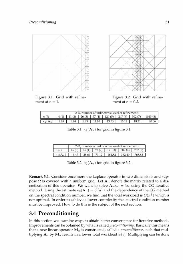
The previous result (3.26) is less interesting than it may seem at first sight. Considerthe Laplace operator, i.e. (3.1) with a = 1 and b = 0, c = 0, in two dimensions.For a uniform grid we have the estimate κ2(An) = O(h−2) = O(n). Numericalobservations show that this estimate is sharp. However, for non-uniform grids thisestimate is not sharp. We demonstrate this for two grids with local refinements asin figures 3.1 and 3.2 by direct computation. In both examples the size of H remainsunchanged and h is halved when an extra level of refinement is added. From (3.23) itwould follow that an extra level of refinement results in an increase of the conditionnumber by a factor 4. However, from table 3.1 we observe that κ2(An)
.= O(l) for a
grid as in figure 3.1; here l is the level of refinement. For the second grid the resultsin table 3.2 seem to indicate that κ2(An)
.= O(n).
Preconditioning 31
Figure 3.1: Grid with refine-ment at x = 1.
Figure 3.2: Grid with refine-ment at x = 0.5.
2-D, number of unknowns (level of refinement)n (l) 4 (1) 11 (2) 26 (3) 57 (4) 120 (5) 247 (6) 502 (7) 1013 (8)
κ2(An) 2.89 5.44 8.29 11.10 13.73 16.11 18.21 20.06
Table 3.1: κ2(An) for grid in figure 3.1.
2-D, number of unknowns (level of refinement)n (l) 16 (0) 45 (1) 93 (2) 191 (3) 389 (4) 787 (5)
κ2(An) 9.47 28.69 71.12 164.82 362.40 768.83
Table 3.2: κ2(An) for grid in figure 3.2.
Remark 3.4. Consider once more the Laplace operator in two dimensions and sup-pose Ω is covered with a uniform grid. Let An denote the matrix related to a dis-cretization of this operator. We want to solve Anxn = bn using the CG iterativemethod. Using the estimate κ2(An) = O(n) and the dependency of the CG method
on the spectral condition number, we find that the total workload is O(n32 ) which is
not optimal. In order to achieve a lower complexity the spectral condition numbermust be improved. How to do this is the subject of the next section.
3.4 Preconditioning
In this section we examine ways to obtain better convergence for iterative methods.Improvements can be obtained by what is called preconditioning. Basically this meansthat a new linear operator Mn is constructed, called a preconditioner, such that mul-tiplying An by Mn results in a lower total workload w(ε). Multiplying can be done

32 Chapter 3: Iterative methods and preconditioners
either from the right or from the left. In order to do so, it is necessary that both theconstruction of and the multiplication by Mn is relatively cheap. In the followingwe first describe how to use such a preconditioner in general. Then we give a sur-vey of existing techniques. This starts with methods that result in an optimal orderworkload, followed by other techniques resulting in suboptimal order.
3.4.1 Preconditioning methods
Two classes of methods for the construction of a preconditioner Mn can be distin-guished: explicit methods and implicit methods. For explicit methods we compute anapproximation Mn to A−1
n , and solve the preconditioned linear system
(3.27) MnAnxn = Mnbn.
Since both Mn and An are explicitly available, only matrix-vector multiplicationsare required in iterations. Alternatively we can solve a right preconditioned linearsystem
(3.28) AnMnyn = bn, xn = Mnun.
For implicit methods Mn approximates An. This gives the preconditioned system
(3.29) M−1n Anxn = M−1
n bn.
Here it is seen that in an iterative method each matrix-vector multiplication requiresthe solution of a linear system involving Mn. The necessity of cheaply solving asystem with M−1
n in order to optimize the workload is evident. We also have theright preconditioned version, i.e.
(3.30) AnM−1n yn = bn, xn = M−1
n yn.
For completeness we mention another variant of preconditioning, viz. one that pre-serves symmetry in case An itself is symmetric. In this situation Mn is available in afactored form, i.e.
Mn = LnLTn .
The preconditioner is then split between left and right, and the system to solve be-comes:
(3.31) L−1n An(L−1
n )Tyn = L−1n bn, xn = (L−1
n )Tyn.
Despite the various ways to create a new, preconditioned, linear system of equations,the goal is to achieve a better conditioned linear operator such that iterative methodsconverge in less steps. For methods depending on the spectral condition number ofthe matrix this means (for (3.29))
(3.32) κ2(M−1n An) κ2(An)
asymptotically in n. Of course, provided construction of and multiplication by Mn
is cheap.
Preconditioning 33
3.4.2 Optimal order techniques for diffusive problems
Consider the situation of a uniformly refined grid, such that the ratio H/h is fixedfor each grid level. These methods are all of multilevel type, and the most importantones are:
• The Algebraic Multi-level Iterative (AMLI) methods. First appeared in [7, 8];
• The Bramble, Pasciak and Xu (BPX) preconditioner. Published in [24];
• Multigrid methods. See for example [25].
Despite many differences all three methods employ a breakdown of the finest gridinto coarser grids. This results in a recursive structure of the preconditioner. Thebasic idea is that a specific relation between two successive levels of refinement, cq.grids, is exploited and used to represent the solution in terms of this breakdown inrefinement levels.Recursion in the sense of exploiting self-similar substructures was used in Chapter 2,which resulted in a nearly optimal order method (O(n logn). In Chapter 5 a recursivenature of grids is exploited as well in a very straightforward manner. This results ina nearly optimal order method as well.
Secondly there are optimal order methods for non-uniform grids where H/h → ∞with increasing level of refinement. These are also of the multilevel type:
• Related to the AMLI method is a method that make use of special 2-d bisectionrefinement for AMLI permitted coarse grids. See [66];
• For the BPX method non-uniform grids are also allowed. However, bisectionrefinement is not allowed, and only the highest level element can be furtherrefined. See [19, 35].
It should be noted that the type of refinement used is important for both methods.
Remark 3.5. Optimal order methods can be used for non-symmetric and indefiniteelliptic problems too. There exists an extensive literature on such problems. In [41]a two-level preconditioner for grids with local refinement is constructed. Under theassumptions that the coarse grid size H is small enough, and that the ratio H/h isbounded, an optimal order preconditioner can be obtained.Multigrid is also employed for non-symmetric and indefinite elliptic problems andhas been extensively studied; see for example [21, 23, 32, 33, 88, 108]. One of therecurring assumptions is that the coarsest grid is sufficiently fine in order to ensurea uniform convergence rate. It also appears that computation of the restriction andprolongation operators are more costly than solving the original problem.
Remark 3.6. Unfortunately, there are situations when optimal order preconditionerscannot be employed. In those situations one has to revert to preconditioning meth-ods that are suboptimal. For symmetric elliptic boundary value problems in a finiteelement context, a preconditioner based on domain decomposition was introduced

34 Chapter 3: Iterative methods and preconditioners
in [22]. This method, called BPS, has the following estimate of the condition numberof the preconditioned system
κ(M−1n An) = O(1 + (ln(H/h))2).
Here H denotes the size of the subdomains, and h is the mesh-size.
3.4.3 Incomplete factorization methods
An important class of preconditioners are the incomplete factorizations methods. Thesepreconditioners are based on direct solution methods (cf. Chapter 2), where part ofthe computation is skipped. This results in incomplete factors Ln and Un such thatLnUn ≈ An. These are then employed as preconditioners as in (3.31). For literaturesee [74] and [31, 75, 84, 103, 104].
Given the incomplete calculation of the factors Ln and Un, a lot of different strate-gies have been studied. The most straightforward strategy is to compute factors thathave the same sparsity pattern S as An. This method is called ILU(0). An imme-diate improvement over ILU(0) are techniques that allow fill-in according to certaincriteria. An approach is to allow fill-in at certain positions such that it leads to morenon-zero bands in the factors. This is similar to omitting fill-in when the fill-in is out-side a prescribed sparsity pattern, which is called the drop by position strategy. Thesemethods are called ILU(p) were p denotes the level of fill-in allowed. Besides drop-ping fill-in based on a criteria for the position of fill-in, fill-in can also be omitted if itsabsolute value is below a certain threshold τ , which is a drop by size strategy. Thesemethods are referred to as ILU(τ ) or ILUT, where the τ denotes the threshold.
Finally we mention the Modified ILU (MILU) method ([49]), which employs a formof additional correction to the diagonal entries. This correction leads to LnUnwn ≈Anwn for almost constant wn. The efficiency of the MILU method strongly dependson the amount of correction applied (see [101]). Let 0 ≤ α ≤ 1 be a parametersteering the amount of correction. For α = 0 we obtain the ILU(0) method and α = 1results in the standard MILU method. Experiments indicate the α = .95 leads to avery substantial reduction in the number of iterations. Of interest is to note that theMILU method is employed as smoother for multigrid methods (see [90, 106]).
3.5 Approximate inverse preconditioning
In the previous section we gave a summary of few of the most well known (implicit)preconditioning methods. In this section we look at explicit preconditioners. Al-though implicit preconditioners have been successfully employed in a number ofapplications, there are two main reasons to examine explicit preconditioners. First ofall, with the introduction of high-performance architectures straightforward imple-mentation of implicit preconditioners could lead to lowering of performance. Espe-cially ILU-type preconditioners are troublesome to implement in parallel, because ofthe recursive nature of the computation. Another drawback of ILU-type precondi-tioners is the possibility of breakdowns during the factorization process, due to zero
Approximate inverse preconditioning 35
pivots. This typically occurs when the matrix An is non-symmetric and/or indefi-nite. Even if some care is taken during the factorization, there is no guarantee thatthe resulting preconditioners will work properly.
A viable alternative is to construct a preconditioner Gn that is an approximationto A−1
n . As mentioned in Subsection 3.4.1 this preconditioner requires only matrix-vector multiplications. Added benefit is that matrix-vector multiplications are wellsuited for parallelism. Ideally, we would like Gn to resemble A−1
n as much a pos-sible, as this obviously would result in a preconditioned linear system that is closeto the identity matrix. However, the inverse of a sparse matrix An is full in general,which necessitates a more careful approach in the construction of such an explicitpreconditioner. These considerations have led to the development of so-called ap-proximate inverse preconditioners. Basically the approximate inverse is constructedby minimizing a consistent norm of the difference between the identity In and thepreconditioned linear system. The motivation for looking at such preconditioners isthe following:For the continuous differential and boundary operators L and B respectively, theGreen’s functions give a representation of the inverse operator. So, intuitively, dis-crete versions of the Green’s functions will be good approximations to A−1
n whereAn is a discretization of L and B. However there are several restrictions. Green’sfunctions are rarely available in closed form. Even if an explicit formula for theGreen’s functions is available, a discrete version, for example by sampling, is notalways beneficial. One major reason is that Green’s functions have global supportwhich will result in a full approximate inverse whereas an efficient preconditionershould be sparse. Also, in two dimensions Green’s functions have a singularity atthe source point, which makes sampling more difficult. The problem of a full ap-proximate inverse may be avoided by sampling the Green’s function in few pointsonly, so that a sparse approximate inverse is obtained. However, this turns out notto be satisfactory either. Yet, let us call the approximate inverse Gn. For simplicitywe will also call this matrix the Green’s matrix.
In the following, we discuss several approximate inverse strategies, but only themost relevant details are given. Most, if not all, literature on approximate inversesdeals with implementation and application only, which in fact means a lack of the-oretical results. The method as such, however, is important for our discussion. InChapter 4 we will discuss our choice of Gn in greater detail.
3.5.1 Frobenius norm minimization
Historically Frobenius norm minimization is the first approximate inverse techniquethat was proposed (see for instance [12]). The main idea is to compute a sparsematrix Gn ≈ A−1
n as the solution of the constrained minimization problem
(3.33) minGn∈Sn
‖In −AnGn‖F .
Here Sn denotes a set of sparse matrices with sparsity pattern S, and ‖ · ‖F denotesthe Frobenius norm. Let ei denote the ith column of In and gi the ith column of Gn.
36 Chapter 3: Iterative methods and preconditioners
Since
‖In −AnGn‖2F =
n∑
i=1
‖ei −Angi‖22,
the minimization problem (3.33) to compute Gn is replaced by solving n distinctlinear least squares problems, each with constraints on the sparsity of gi. In order tocompute the gi we minimize
‖ei −Angi‖22
given the sparsity pattern for gi. This boils down to solving
(3.34) [Angi]j = [ei]j , (j, i) ∈ S.
This method has the highest potential for parallelism. The approximate inverse tech-nique described in Chapter 4 is based on Frobenius norm minimization and solv-ing (3.34) for obtaining Gn in particular.
This Frobenius norm minimization can be generalized into a weighted variant (see [4]).Given a symmetric positive definite matrix Hn, the norm to be minimized is
(3.35) ‖In −AnGn‖2FH
≡ tr((In −AnGn)Hn(In −AnGn)T ).
The n linear systems needed to compute the columns of Gn are
ATnHnAngi = AT
nHnei, i = 1, . . . , n.
Clearly, Hn = In gives back (3.33).If An is symmetric positive definite, with Hn = A−1
n the approximate inverse Gn
satisfies[AnGn]i,j = δi,j , (i, j) ∈ S.
One of the important issues is the choice of the sparsity pattern S. If S is given orknown a priori, then computation of Gn is straightforward. This computation ishighly parallelizable since the computation of gi is a local process only.The role of S is intended to remove small entries of A−1
n , and retain the large entries,that influence the quality of the preconditioner. However, for an arbitrary sparsematrix it is not known in advance which entries of its inverse are large. This makesthe choice of S difficult. In order to overcome this problem, a common choice is totake the sparsity pattern of An for S. If there are still large elements in A−1
n locatedoutside the non-zero pattern of An, another choice is to take the sparsity patternof Ap
n, p ≥ 2. In general this means that more information of A−1n is captured in
the approximate inverse Gn. However, there is no guarantee it will work properly.Also the cost for computing and storing the approximate inverse grows rapidly forincreasing p.As the problem of prescribing a good sparsity pattern S for Gn remained, adaptivestrategies have been developed, see [34, 47]. The approach in [47] is probably themost successful and is better known as the SParse Approximate Inverse (SPAI) precon-ditioner. The strategy is to start with an initial sparsity pattern and to enlarge it when

Approximate inverse preconditioning 37
entries found outside the sparsity pattern at that moment are considered to be largeaccording to some threshold. See [17, 47] for more details of the SPAI preconditioner.
3.5.2 Factorized sparse approximate inverses
A big disadvantage of the Frobenius norm based approximate inverse is that Gn
does not preserve symmetry and/or positive definiteness of An in general, even ifAn is. This means it cannot be used with the CG method to solve symmetric positivedefinite problems. We consider therefore a method that does have this property. Itis based on computing a factorized sparse approximate inverse using incompleteinverse factorizations.Assume that An can be factored as LnDnUn where Ln is lower triangular, Dn is di-agonal and Un is upper triangular. Then A−1
n = U−1n D−1
n L−1n . The factorized sparse
approximate inverse is constructed by computing its factors Zn and Wn which aresparse approximations to U−1
n and L−1n respectively. Then as approximate inverse
we take
(3.36) Gn = ZnD−1n Wn.
Several approaches have been developed to compute the approximate factors Znand Wn.A first class of methods does not need a factorization of An, but constructs the fac-torized approximate inverse directly from An. This includes the Factorized SparseApproximate Inverse (FSAI) method introduced in [60] which can be described as fol-lows. Assume that An is symmetric positive definite, and let SL denote a prescribedlower triangular sparsity pattern including the main diagonal. Then the lower trian-
gular matrix Zn is computed by solving
(3.37) [AnZn]i,j = δi,j , (i, j) ∈ SL.
Let Dn := (diag(Zn))−1 and Zn = D1/2n Zn, then the preconditioned linear system
ZnAnZTn is symmetric positive definite, and diagonal entries equal to 1. A common
choice for SL is to take
(3.38) SL := (i, j) : [An]i,j 6= 0, i ≥ j,
i.e. the non-zeros in the lower triangular part of An. For a better approximation,albeit at a higher cost, another choice is to take the non-zeros in the lower triangularpart of Ap
n for p ≥ 2. The main drawback of FSAI is that it relies on a prescribedsparsity pattern, and is not well suited for general sparse matrices. The method canbe extended to the case of non-symmetric matrices. However, the solvability of thelocal linear systems and the non-singularity of the approximate inverse is no longerguaranteed.
A second method of computing a factorized approximate inverse is discussed in [14].The advantage of this method is that a prescribed sparsity pattern is not required.
38 Chapter 3: Iterative methods and preconditioners
This method is based on incomplete (bi)conjugation and generally referred to asAINV. The algorithm computes two sets of vectors, wini=1, zini=1 that are An-biconjugate, i.e.
(3.39) zTi Anwj = 0 ⇔ i 6= j.
LetZn = [z1, . . . zn], and Wn = [w1, . . .wn, ]
then
(3.40) WTnAnZn = Dn = diag(p1, . . . , pn)
wherepi = wT
i Anzi 6= 0.
Wn and Zn are non-singular and hence
A−1n = ZnD
−1n WT
n
which gives us a factorization of A−1n .
In general Zn and Wn are dense, and to get a sparse approximate inverse, the ma-
trices Zn and Wn are computed incompletely. This gives incomplete factors Zn, Wn
and an approximation Dn ≈ Dn. The factorized approximate inverse takes the form
Gn = ZnD−1n WT
n . The advantage of factorized sparse approximate inverse tech-niques over the SPAI technique in Subsection 3.5.1 is that the former can be used aspreconditioners for the CG method for solving symmetric positive definite problems.
3.5.3 Practical use of approximate inverses
We conclude this section with some comments on the use of the approximate in-verse preconditioning techniques. As has been mentioned before, the approximateinverses were developed to overcome breakdown of preconditioners such as theILU(0). As such the setting in which approximate inverses are presented in liter-ature is rather practical and implementation oriented. In [15] several tests weredone to compare the ILU(0) and the SPAI and AINV as preconditioner. The exper-iments were performed on sparse matrices, mostly from the Harwell-Boeing collec-tion. These non-symmetric matrices originate from a wide range of applications suchas oil reservoir simulation and circuit design. Several observations can be made.AINV and SPAI fail for a few test problems, but for the remainder of the tests the ro-bustness of the AINV and SPAI is comparable with the ILU(0). Rates of convergenceare also comparable; AINV seems to perform a bit better than SPAI. The time for theiterative part however, shows that SPAI and AINV are much better than ILU(0) dueto the good vectorization properties of the approximate inverses. The price to payis the expensive construction time for SPAI and AINV with the first one being evenmuch more expensive than the latter. It should be noted that SPAI was designed forparallel implementations which has not been taken into account in these tests. Forother tests in different settings see for instance [13, 14, 16, 34].
Diagonal approximate inverses 39
3.6 Diagonal approximate inverses
In the discussion of the choice for S, we mentioned that the sparsity pattern of An isa common choice, or alternatively that of Ap
n for p ≥ 2. It is also possible to constructa diagonal approximate inverse, which, in fact, inherits the sparsity patter of A0
n. Letthis diagonal approximate inverse be denoted by Dn. For right preconditioning weobserve that the columns of AnDn are scaled versions of the columns of An since[AnDn].,j = [An].,j [Dn]j,j . Similarly, for the left preconditioned system DnAn therows are scaled. With such scalings it is possible to lower the condition number ofAn. This is called equilibration and has been studied in considerable detail in [10, 98,100, 99].From [98] we derive several results on what can be obtained optimally with equili-bration: Let ‖ · ‖p be be any Holder norm, p > 0 or p = ∞, or the Frobenius norm.For the left preconditioned linear system we then have
Theorem 3.7. Let κ(An) = ‖An‖∞‖A−1n ‖p. Then for a diagonal matrix Dn, κ(DnAn)
is minimal if in DnAn all rows have identical 1-norm.
For the right preconditioned case:
Theorem 3.8. Let κ(An) = ‖An‖1‖A−1n ‖p. Then κ(AnDn) is minimal if in AnDn all
columns have identical 1-norm.
However, in practice we are more interested in the spectral condition number κ2 ofthe matrix. Then, based on 1√
n‖ · ‖∞ ≤ ‖ · ‖2 ≤ √
n‖ · ‖∞, we have
Corollary 3.9. Let κ(An) = ‖An‖2‖A−1n ‖p and let Dn denote the set of n × n diagonal
matrices. Thenκ(DnAn) ≤
√n min
Dn∈Dn
κ(DnAn)
if all rows in DnAn have identical 2-norm, and
κ(AnDn) ≤√n min
Dn∈Dn
κ(AnDn)
if all columns in AnDn have identical 2-norm.
For sparse matrices that are symmetric positive definite the last result can be refined(see [98]):
Corollary 3.10. Let An be symmetric positive definite and κ(An) = ‖An‖2‖A−1n ‖2. As-
sume that An has at most m non-zeros in any row. Then
κ(An) ≤ m minDn∈Dn
κ(DnAnDn)
if the main diagonal of An is constant.
In [98] no information is provided about the optimality of Dn. These results indicatethat diagonal preconditioning is most efficient when this preconditioner equilibratesthe rows or columns of the given linear operator An.

Chapter 4
The approximate inverse
In this chapter we look further into the approximate inverse technique introduced inSection 3.5. In the first section we consider a discretization for a general convectiondiffusion equation on a non-uniform grid. For a certain class of tridiagonal matrices,which also arise from the previously discussed discretizations, the eigenvalues andeigenvectors can be determined. This theory leads to Toeplitz matrices which areone of the few types of matrices for which the spectrum, and henceforth the spectralcondition number, can be computed.
The spectral condition numbers of our preconditioned linear systems AnGn andGnAn are difficult to compute, since they are not symmetric. However, as it turnsout, these preconditioned linear systems resemble a Toeplitz matrix. For the onedimensional case we alter the approximate inverse based preconditioner such thatthe products AnGn and GnAn are Toeplitz for the pure diffusive problems. UsingToeplitz matrix results summarized in [20] the spectral condition number can be de-rived. For the product GnAn we give an estimate of the spectral condition number,since in this case the inverse is explicitly known. The spectral condition number ofthe other product AnGn is estimated in an alternative way, which is described at theend of the chapter.
4.1 The convection diffusion discretization
Let a, b and c be non-negative real numbers, g a function, and consider the BVP:
−ad2u
dx2+ b
du
dx+ cu = g(x), x ∈ Ω = (0, 1),
u(0) = u(1) = 0.
Let n be a positive integer, let ψ ∈ (0, 1]. Define f := 1/ψn+1 and F the mapping
(4.1) F : x 7→ f (1−x) − f
1 − f.

42 Chapter 4: The approximate inverse
Finally, let
(4.2) xi := F (i/(n+ 1)) =f (1−i/(n+1)) − f
1 − f, ∀i = 0, . . . , n+ 1.
Then x0 = 0, xn+1 = 1, and
(4.3) ψ =xi+1 − xixi − xi−1
, ∀i = 1, . . . , n.
Indeed,
xi+1 − xixi − xi−1
=f1−(i+1)/(n+1) − f1−i/(n+1)
f1−i/(n+1) − f1−(i−1)/(n+1)=f1−1/(n+1) − f
f − f 1+1/(n+1)
=f−1/(n+1) − 1
1 − f 1/(n+1)=
ψ − 1
1 − ψ−1
=ψ
ψ
ψ − 1
1 − ψ−1= ψ
ψ − 1
ψ − 1= ψ.
Thus grid points xi are denser for xi close to 1. Define
(4.4) hi := xi+1 − xi, ∀i = 0, . . . , n,
and let
(4.5) H := h0 and h := hn,
thenxi+1 − xixi − xi−1
= ψ ⇒ hi = ψiH, ∀i = 0, . . . , n.
Thus,h = ψnH.
If we take Ω = (α, β), then H can simply be found, for
β−α =
n∑
i=0
(xi+1 −xi) =
n∑
i=0
hi =
n∑
i=0
ψiH = H · 1 − ψn+1
1 − ψ⇒ H = (β−α)
1 − ψ
1 − ψn+1.
Now we proceed as follows: Let ui.= u(xi). Using (4.3), we find
xi−1 = xi − hi/ψ, xi+1 = xi + hi.
Using a Taylor expansion and a bit of algebra, a central difference approximation ofu 7→ u′′ is (see [69])
2
hi−1 + hi
(
ui+1 − uihi
− ui − ui−1
hi−1
)
.= u′′(xi) ⇒
1
h2i
2ψ
1 + ψ(ψu(x− hi/ψ) − (1 + ψ)u(x) + u(x+ hi)) = u′′(xi) +O(hi).

Eigenvalues and eigenvectors of tridiagonal matrices 43
Thus discretizing the operator u 7→ −au′′ results in the difference equation
1
h2i
· 2ψ
1 + ψ· a (−ψui−1 + (1 + ψ)ui − ui+1) .
The related stencil is given by
1
h2i
· 2ψ
1 + ψ· a [−ψ, (1 + ψ),−1] , ∀i = 1, . . . , n.
For a first order downwind discretization of u 7→ bu′ the stencil is
1
hi· b [−1, 1, 0] .
Thus, the stencil for the finite difference operator is given by
(4.6)1
h2i
· 2ψ
1 + ψ· a [−ψ, (1 + ψ),−1] +
1
hi· b [−1, 1, 0] + c [0, 1, 0] , i = 1, . . . , n.
After using the boundary values for u0 and un+1 we can collect these differenceequations in the usual way in a matrix An.
4.2 Eigenvalues and eigenvectors of tridiagonal matrices
In this section we compute the eigenvalues and eigenvectors related to the discretiza-tion of convection and diffusion.
First, consider forward differences: Then An ∈ Rn×n is typically given by
An =
a0 a1
0 a0 a1
. . .. . .
. . .
0 a0 a1
0 a0
, a0, a1 ∈ R, a1 6= 0.
Clearly, An resembles a Jordan matrix in a trivial way. Its eigenvalue is a0 (algebraicmultiplicity n), and its single eigenvector is e1 := [1, 0, . . . , 0]T (geometric multiplic-ity 1).
Next consider backward differences: Then a typical form of An is
An =
a0 0a−1 a0 0
. . .. . .
. . .
a−1 a0 0a−1 a0
, a−1, a0 ∈ R, a−1 6= 0.
44 Chapter 4: The approximate inverse
Here An is again similar to a Jordan matrix. Its eigenvalue is a0 (algebraic multi-plicity n), and its single eigenvector is en := [0, . . . , 0, 1]T (geometric multiplicity1).
To finish with, we consider central differences for the double derivative:For some a−1, a0, a1 ∈ R, a−1 6= 0, a1 6= 0, and An ∈ Rn×n typically has the form
An =
a0 a1
a−1 a0 a1
. . .. . .
. . .
a−1 a0 a1
a−1 a0
.
For this tridiagonal matrix we can find the eigenvalues and eigenvectors as follows.Let λ ∈ R and xn = [x1, . . . , xn]T ∈ Rn be such that Anxn = λxn. Then
a0x1 + a1x2 = λx1,a−1xk−1 + a0xk + a1xk+1 = λxk, k = 2, . . . , n− 1,a−1xn−1 + a0xn = λxn.
Introducing x0 = xn+1 = 0, we find that xkn+1k=0 satisfies the recurrence relation
(4.7)
x0 = 0,a−1xk−1 + (a0 − λ)xk + a1xk+1 = 0, k = 1, . . . , n.xn+1 = 0.
Using this relation, we proceed as follows. The characteristic polynomial of the re-cursion is
x2 +a0 − λ
a−1x+
a1
a−1= 0.
First let the roots λ1 and λ2 of the characteristic polynomial be different. Then thereare α1, α2 ∈ R, so that the solution of (4.7) is given by
xi = α1λi1 + α2λ
i2, i = 0, . . . , n+ 1.
Using the fact that x0 = xn+1 = 0 we find
xn+1 = α1
(
λn+11 − λn+1
2
)
= 0.
Note that α1 = −α2 = 0 would correspond to the trivial solution, which we thereforeexclude.Hence
λn+11 = λn+1
2 ⇒(
λ1
λ2
)n+1
= 1 ⇒ λ1
λ2= e2πi·
pn+1 = e
2pπi
n+1 .
Using λ1λ2 = a1/a−1, i.e.,
λ21 = λ1λ2 ·
λ1
λ2= a1/a−1 · e
2pπi
n+1 ,

The spectral condition number of Toeplitz matrices 45
we findλ1 = ±
√
a1/a−1 · epπi
n+1
λ2 = ±√
a1/a−1 · e−pπi
n+1 .
Since
a0 − λ
a−1= −(λ1 + λ2) = −±
√
a1/a−1 · 2 cos(pπ
n+ 1)
we obtainλ = a0 ± 2
√a−1a1 cos(
pπ
n+ 1).
If a1/a−1 < 0 we have complex eigenvalues, viz.
λ = a0 + 2i ·√
|a−1a1| cos(pπ
n+ 1).
Finally λ1 = λ2 cannot occur as this would imply that xi = (α1 + α2 · i)λi1, i.e.,α1 = α2 = 0 ⇒ x = 0.The above results are summarized in the following corollary.
Corollary 4.1. For a−1a1 6= 0:
(4.8)
σ(An) =(
a0 + 2√a−1a1 cos( pπ
n+1 ))n
p=1
⊂ (a0 − 2√a−1a1(1 − 2
(
πn+1
)2
+O( πn+1 )4), a0 + 2
√a−1a1)
⊂ (a0 − 2√a−1a1, a0 + 2
√a−1a1).
The related eigenvectors xp are:
xp =
(
√
(a1/a−1)isin(
πp
n+ 1i)
)n
i=0
.
4.3 The spectral condition number of Toeplitz matrices
In this section we summarize a number of properties for so called Toeplitz matrices.For a state of the art overview of properties see [20]. For Toeplitz matrices the spectralcondition number can be computed with the use of the ‖ · ‖∞ norm. This is themain result of interest in relation to the approximate inverse preconditioner, whichis discussed in the next section.
Definition 4.2. Let b := (. . . , b−2, b−1, b0, b1, b2, . . .)T ∈ R∞, a real vector in l1. The
infinite matrix Bn defined by
Bn =
b0 b1 b2 . . .b−1 b0 b1 . . .b−2 b1 b0 . . .
......
.... . .
is called a Toeplitz matrix. The numbers . . . , b−2, b−1, b0, b1, b2, . . . do not depend on n.
46 Chapter 4: The approximate inverse
A finite section of a Toeplitz matrix, i.e. the matrix (see [20, (2.5)])
Bn =
b0 b1 . . . bn−1
b−1 b0. . .
......
. . .. . . b1
b−n+1 . . . b−1 b0
, bi ∈ R,
is also called a Toeplitz matrix.For Toeplitz matrices the spectral condition number can be computed using the ‖·‖∞norm. This is due to a special relation between the largest and smallest singularvalues σ1(Bn) and σn(Bn) of a matrix Bn on the one hand and the values of ‖Bn‖∞and ‖B−1
n ‖∞ on the other hand respectively.For the largest singular value we have (see [20, (2.5) and Theorem 4.13])
Theorem 4.3. For b ∈ l1 the following holds
(4.9) limn→∞
σn(Bn) = limn→∞
||Bn||∞ =
∞∑
i=−∞
|bi|.
There is a similar result for the smallest singular value σ1 (see [20, Theorem 4.3 (4.8)])
Theorem 4.4. If σ1(Bn) is such that for all n ∈ N, σ1(Bn) ≥ δ > 0 then
(4.10) limn→∞
σ1(Bn) = limn→∞
1
||B−1n ||∞
.
Therefore, if Bn is Toeplitz, we have
limn→∞
κ2(Bn) = limn→∞
σn(Bn)
σ1(Bn)=
limn→∞ σn(Bn)
limn→∞ σ1(Bn)=
∞∑
i=−∞
|bi|/ limn→∞
‖B−1n ‖∞.
Example 4.5. The matrix [−1, 2,−1] has singular values that are equal to some of itseigenvalues (see (4.8)) of which the largest one converges to 4 for n→ ∞.
Example 4.6. In the case of no refinement (i.e. ψ = 1) we have hi = H = h =1/(n+ 1). Then the matrix An based on (4.6) is Toeplitz,
An =1
h2· a [−1, 2,−1] +
1
h· b [−1, 1, 0] + c [0, 1, 0]
= [− a
h2− b
h, 2
a
h2+b
h+ c,− a
h2],
for each value of n. However we have An 6= ATn , so κ2(An) is not simple to compute.
From (4.8) we find that
σ(An) =
(
2a
h2+b
h+ c+ 2
1
h2
√
(a2
h2+ab
h) cos(
pπ
n+ 1)
)n
p=1
.
A preconditioner based on approximate inverses 47
However,κ2(An) = σn(An)/σ1(An),
where σ1 ≤ σ2 ≤ ... ≤ σn are the singular values of An (positive square roots ofeigenvalues of AnA
Tn ) are not known – because An is not symmetric. The theorems
stated above cannot be used because the entries of An depend on n. For fixed n andrefinement (ψ < 1) the matrix An does not have constant diagonals and cannot becalled Toeplitz.
4.4 A preconditioner based on approximate inverses
Now consider the application of the approximate inverse technique using Frobeniusnorm minimization that was introduced in Subsection 3.5.1. This technique calcu-lates a preconditioner Gn such that AnGn approximates In given a certain sparsitypattern S that Gn should satisfy. First we describe computation of Gn for a gen-eral sparsity pattern, and introduce necessary notations. Then, for the convectiondiffusion operator we examine the structure of Gn in detail where Gn inherits thesparsity structure of An. For the pure diffusion case AnGn is almost Toeplitz. Wecompute a sparse matrix Gn such that AnGn approximates In and is Toeplitz. Forthis product we calculate the spectrum and spectral condition number.
Let S be a given sparsity pattern. Then in order to compute the columns of Gn wehave to solve
[Angi]j = [ei]j , (j, i) ∈ S, i = 1, . . . , n.
Let Si denote the sparsity pattern of gi, i.e.,
Si := j : (j, i) ∈ S,
and let its elements be numbered as j1, . . . , jmi . Let A(i) be an mi×mi sub-matrix ofAn, defined by
[A(i)]p,q := [An]jp,jq , p, q = 1, . . . ,mi,
and likewise let e(i) be the unit vector of dimension mi given by
[e(i)]p := δjp,i, p = 1, . . . ,mi.
Then solving the large n × n linear system reduces to solving the mi × mi linearsystem
A(i)g(i) = e(i), i = 1, . . . , n.
Provided that A(i) is non-singular we thus obtain a vector g(i). This shows that ifi 6∈ Si, e(i) = 0 and hence gi = 0 as well. So we may assume that i ∈ Si.From g(i) we construct gi via
[gi]jp =
[g(i)]p if jp ∈ Si,
0 otherwise.
48 Chapter 4: The approximate inverse
Finally, the approximate inverse, the Green’s matrix, Gn is constructed with the gias its columns, and Gn satisfied the prescribed sparsity pattern S.
In order to compute the approximate inverse of (4.6) we take
S = (i, j) : [An]i,j 6= 0.
Since An is tridiagonal, we have to consider only the equations for xi, xi−1 and xi+1.For computing the ith column of Gn we have to solve A(i)g(i) = e2. Here A(i) is the3× 3 sub-matrix of An, and g(i) a vector related to node i as explained in Section 3.5.Since hi−1 = hi/ψ and hi+1 = hiψ we have to solve a system dependent on hi only:
c+ 2 a ψ3
h2i
+ b ψhi
−2 a ψ3
(1+ψ)h2i
0−2 a ψ2
(1+ψ)h2i− b
hic+ 2 aψ
h2i
+ bhi
−2 aψ(1+ψ)h2
i
0 −2 a(1+ψ)h2
i− b
ψ hic+ 2 a
ψ h2i
+ bψ hi
g(i) =
010
.
Except for i = 1 and i = n we find
g(i) =
2 aψ2 (2 a+hi (b+cψ hi))(1+ψ)h4
i
(2 a ψ3+hi (b ψ+c hi)) (2 a+hi (b+cψ hi))
ψ h4i
(2 a ψ+b (1+ψ)hi) (2 aψ3+hi (b ψ+c hi))ψ (1+ψ)h4
i,
/det(A(i)).
The vector g(1) related to node 1 is found by solving the 2× 2 linear system of equa-tions
[
c+ 2 aψh21
+ bh1
−2 a ψ(1+ψ)h2
1−2 a
(1+ψ) h21− b
ψ h1c+ 2 a
ψ h21
+ bψ h1
]
g(1) =
[
10
]
,
and likewise for g(n) related to node n we have to solve
[
c+ 2 aψ3
h2n
+ b ψhn
−2 aψ3
(1+ψ)h2n
−2 a ψ2
(1+ψ)h2n− b
hnc+ 2 aψ
h2n
+ bhn
]
g(n) =
[
01
]
.
We find
g(1) =1
det(A(1))
[
c+ 2 aψ h2
1+ b
ψ h1
2 a(1+ψ) h2
1+ b
ψ h1
]
, and g(n) =1
det(A(n))
[
2 a ψ3
(1+ψ)h2n
c+ 2 aψ3
h2n
+ b ψhn
]
.
We are interested in the matrix AnGn, a five diagonal matrix. In the followingwe have a more detailed look at its entries. The ith column of AnGn is computed
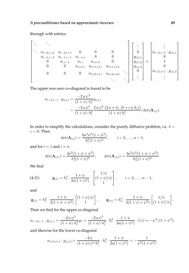
A preconditioner based on approximate inverses 49
through with entries:
. . .. . .
. . . ai−2,i−2 ai−2,i−1 0 0 0ai−1,i−2 ai−1,i−1 ai−1,i 0 0
0 ai,i−1 ai,i ai,i+1 00 0 ai+1,i ai+1,i+1 ai+1,i+2
0 0 0 ai+2,i+1 ai+2,i+2. . .
. . .. . .
·
...0
g(i),1g(i),2g(i),3
0...
=
...ai−2,i−1 · g(i),1
010
ai+2,i+1 · g(i),3...
.
The upper non-zero co-diagonal is found to be
ai−2,i−1 · g(i),1 =−2 aψ5
(1 + ψ) h2i
g(i),1
=−2 aψ5
(1 + ψ) h2i
2 aψ2 (2 a+ hi (b+ c ψ hi))
(1 + ψ)h4i
/det(A(i)).
In order to simplify the calculations, consider the purely diffusive problem, i.e. b =c = 0. Then
det(A(i)) =8a3ψ3(1 + ψ2)
h6i (1 + ψ)2
, i = 2, . . . , n− 1,
and for i = 1 and i = n
det(A(1)) =4a2(1 + ψ + ψ2)
h41(1 + ψ)2
, det(A(n)) =4a2ψ4(1 + ψ + ψ2)
h4n(1 + ψ)2
.
We find
(4.11) g(i) = h2i ·
1 + ψ
2a(1 + ψ2)·
1/ψ(1 + ψ)/ψ
1
, i = 2, . . . , n− 1,
and
g(1) = h21 ·
1 + ψ
2(1 + ψ + ψ2)
[
(1 + ψ)/ψ1
]
, g(n) = h2n · 1 + ψ
2(1 + ψ + ψ2)
[
1/ψ(1 + ψ)/ψ
]
.
Then we find for the upper co-diagonal
ai−2,i−1 · g(i),1 =−2 aψ5
(1 + ψ) h2i
g1 =−2 aψ5
(1 + ψ) h2i
· h2i ·
1 + ψ
2a(1 + ψ2)· 1/ψ = −ψ4/(1 + ψ2),
and likewise for the lower co-diagonal
ai+2,i+1 · g(i),3 =−2 a
(1 + ψ)ψ2 h2i
· h2i ·
1 + ψ
2a(1 + ψ2)= − 1
ψ2(1 + ψ2).
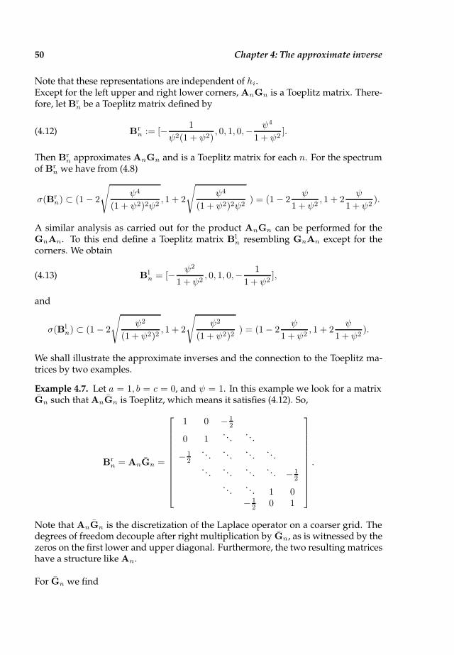
50 Chapter 4: The approximate inverse
Note that these representations are independent of hi.Except for the left upper and right lower corners, AnGn is a Toeplitz matrix. There-fore, let Br
n be a Toeplitz matrix defined by
(4.12) Brn := [− 1
ψ2(1 + ψ2), 0, 1, 0,− ψ4
1 + ψ2].
Then Brn approximates AnGn and is a Toeplitz matrix for each n. For the spectrum
of Brn we have from (4.8)
σ(Brn) ⊂ (1 − 2
√
ψ4
(1 + ψ2)2ψ2, 1 + 2
√
ψ4
(1 + ψ2)2ψ2) = (1 − 2
ψ
1 + ψ2, 1 + 2
ψ
1 + ψ2).
A similar analysis as carried out for the product AnGn can be performed for theGnAn. To this end define a Toeplitz matrix Bl
n resembling GnAn except for thecorners. We obtain
(4.13) Bln = [− ψ2
1 + ψ2, 0, 1, 0,− 1
1 + ψ2],
and
σ(Bln) ⊂ (1 − 2
√
ψ2
(1 + ψ2)2, 1 + 2
√
ψ2
(1 + ψ2)2) = (1 − 2
ψ
1 + ψ2, 1 + 2
ψ
1 + ψ2).
We shall illustrate the approximate inverses and the connection to the Toeplitz ma-trices by two examples.
Example 4.7. Let a = 1, b = c = 0, and ψ = 1. In this example we look for a matrixGn such that AnGn is Toeplitz, which means it satisfies (4.12). So,
Brn = AnGn =
1 0 − 12
0 1. . .
. . .
− 12
. . .. . .
. . .. . .
. . .. . .
. . .. . . − 1
2. . .
. . . 1 0− 1
2 0 1
.
Note that AnGn is the discretization of the Laplace operator on a coarser grid. Thedegrees of freedom decouple after right multiplication by Gn, as is witnessed by thezeros on the first lower and upper diagonal. Furthermore, the two resulting matriceshave a structure like An.
For Gn we find
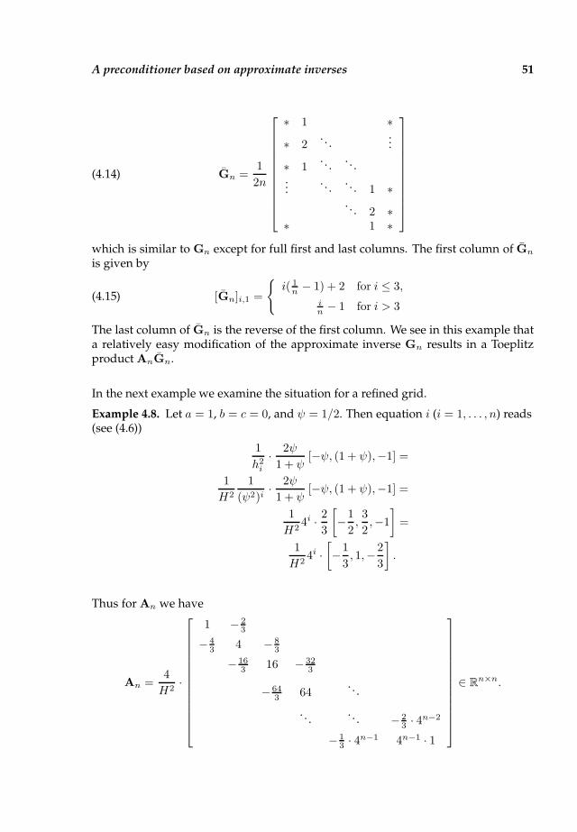
A preconditioner based on approximate inverses 51
(4.14) Gn =1
2n
∗ 1 ∗∗ 2
. . ....
∗ 1. . .
. . ....
. . .. . . 1 ∗. . . 2 ∗
∗ 1 ∗
which is similar to Gn except for full first and last columns. The first column of Gn
is given by
(4.15) [Gn]i,1 =
i( 1n − 1) + 2 for i ≤ 3,
in − 1 for i > 3
The last column of Gn is the reverse of the first column. We see in this example thata relatively easy modification of the approximate inverse Gn results in a Toeplitzproduct AnGn.
In the next example we examine the situation for a refined grid.
Example 4.8. Let a = 1, b = c = 0, and ψ = 1/2. Then equation i (i = 1, . . . , n) reads(see (4.6))
1
h2i
· 2ψ
1 + ψ[−ψ, (1 + ψ),−1] =
1
H2
1
(ψ2)i· 2ψ
1 + ψ[−ψ, (1 + ψ),−1] =
1
H24i · 2
3
[
−1
2,3
2,−1
]
=
1
H24i ·[
−1
3, 1,−2
3
]
.
Thus for An we have
An =4
H2·
1 − 23
− 43 4 − 8
3
− 163 16 − 32
3
− 643 64
. . .
. . .. . . − 2
3 · 4n−2
− 13 · 4n−1 4n−1 · 1
∈ Rn×n.
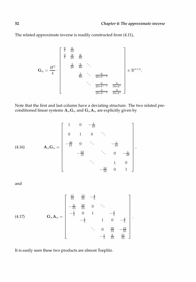
52 Chapter 4: The approximate inverse
The related approximate inverse is readily constructed from (4.11),
Gn =H2
4·
97
620
37
920
680
320
980
. . .
380
. . . 620∗4n−3
. . . 920∗4n−3
656∗2n
320∗4n−3
956∗2n
∈ Rn×n.
Note that the first and last column have a deviating structure. The two related pre-conditioned linear systems AnGn and GnAn are explicitly given by
(4.16) AnGn =
1 0 − 120
0 1 0. . .
− 4821 0
. . . − 120
− 3210
. . . 0 − 128
. . . 1 0
− 3210 0 1
,
and
(4.17) GnAn =
3135
1235 − 4
5
− 635
3935 0
. . .
− 15 0 1 − 4
5
− 15 1 0 − 4
5
. . . 0 3935 − 12
35
− 15
635
3135
.
It is easily seen these two products are almost Toeplitz.
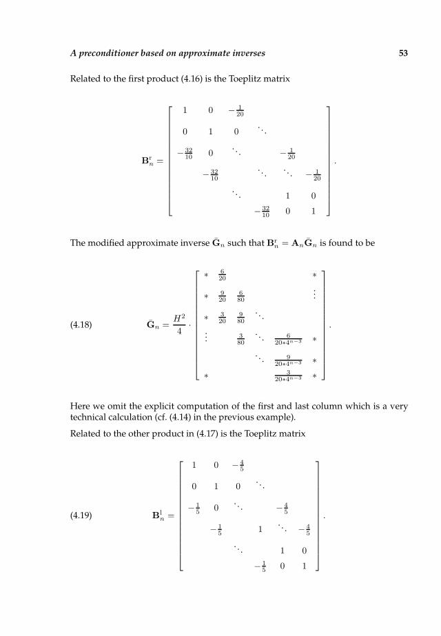
A preconditioner based on approximate inverses 53
Related to the first product (4.16) is the Toeplitz matrix
Brn =
1 0 − 120
0 1 0. . .
− 3210 0
. . . − 120
− 3210
. . .. . . − 1
20
. . . 1 0
− 3210 0 1
.
The modified approximate inverse Gn such that Brn = AnGn is found to be
(4.18) Gn =H2
4·
∗ 620 ∗
∗ 920
680
...
∗ 320
980
. . .
... 380
. . . 620∗4n−3 ∗
. . . 920∗4n−3 ∗
∗ 320∗4n−3 ∗
.
Here we omit the explicit computation of the first and last column which is a verytechnical calculation (cf. (4.14) in the previous example).
Related to the other product in (4.17) is the Toeplitz matrix
(4.19) Bln =
1 0 − 45
0 1 0. . .
− 15 0
. . . − 45
− 15 1
. . . − 45
. . . 1 0
− 15 0 1
.
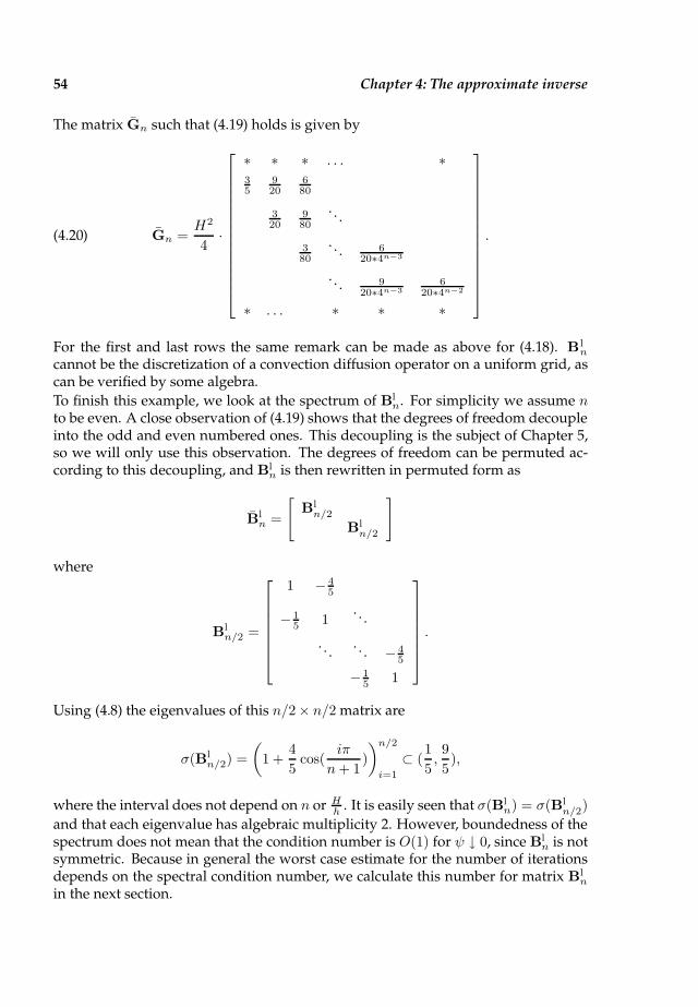
54 Chapter 4: The approximate inverse
The matrix Gn such that (4.19) holds is given by
(4.20) Gn =H2
4·
∗ ∗ ∗ . . . ∗35
920
680
320
980
. . .
380
. . . 620∗4n−3
. . . 920∗4n−3
620∗4n−2
∗ . . . ∗ ∗ ∗
.
For the first and last rows the same remark can be made as above for (4.18). Bln
cannot be the discretization of a convection diffusion operator on a uniform grid, ascan be verified by some algebra.
To finish this example, we look at the spectrum of Bln. For simplicity we assume n
to be even. A close observation of (4.19) shows that the degrees of freedom decoupleinto the odd and even numbered ones. This decoupling is the subject of Chapter 5,so we will only use this observation. The degrees of freedom can be permuted ac-cording to this decoupling, and Bl
n is then rewritten in permuted form as
Bln =
[
Bln/2
Bln/2
]
where
Bln/2 =
1 − 45
− 15 1
. . .
. . .. . . − 4
5
− 15 1
.
Using (4.8) the eigenvalues of this n/2× n/2 matrix are
σ(Bln/2) =
(
1 +4
5cos(
iπ
n+ 1)
)n/2
i=1
⊂ (1
5,9
5),
where the interval does not depend on n or Hh . It is easily seen that σ(Bl
n) = σ(Bln/2)
and that each eigenvalue has algebraic multiplicity 2. However, boundedness of thespectrum does not mean that the condition number is O(1) for ψ ↓ 0, since Bl
n is notsymmetric. Because in general the worst case estimate for the number of iterationsdepends on the spectral condition number, we calculate this number for matrix Bl
n
in the next section.

The spectral condition number related to a refined grid 55
4.5 The spectral condition number related to a refined
grid
In the previous section we found that the preconditioned linear system resembles aToeplitz matrix Bn. However, since both Bl
n and Brn are non-symmetric the spectral
condition number cannot easily be estimated. In [69] it is shown that with the useof Green’s functions certain classes of tridiagonal matrices have inverses that can becomputed explicitly. This comes in handy as the relation (4.10) requires an explicitinverse. Note that the calculation of κ2(B
ln) and κ2(B
rn) require different approaches,
because of different matrix properties.
First we summarize a result from [69]. Let Ω = (0, 1) be partitioned as 0 = x0 < x1 <. . . < xn+1 = 1. Let hi = xi − xi−1. Assume that
u 7→ −d2u
dx2,
is discretized as
(4.21) − 2hi+1
hi+1 + hiui−1 + 2ui −
2hihi+1 + hi
ui+1 = hihi+1f(xi, u(xi), u′(xi)).
Let An ∈ Rn×n be the matrix
(4.22) An = [− 2hi+1
hi+1 + hi, 2,− 2hi
hi+1 + hi].
Then (see [69, Corr. 5.5])
Property 4.9. For the matrix An defined as above, its inverse is explicitly given by
(4.23) [A−1n ]i,j =
hj+1+hj
2hj+1hj(1 − xj)xi, i ≤ j
hj+1+hj
2hj+1hjxj(1 − xi), i ≥ j.
We will use this result to compute the spectral condition number of Bln, without
convection, related to a refined grid with refinement factor ψ. Since the above resultholds for tridiagonal matrices, we assume that Bl
n has been permuted and parti-tioned, i.e.,
(4.24) Bln =
[
Bln/2
Bln/2
]
.
So in the following we estimate the spectral condition condition for Bln/2, which, of
course, is equal to that of Bln itself. From the construction of Bl
n in (4.13), there existb−1 and b1 such that
Bln/2 = [
b−1
2, 1,
b12
].
Then for (Bln/2)
−1 we have

56 Chapter 4: The approximate inverse
Property 4.10. Let ψ ≤ 1 and Ψ := ψ2. Then Bln/2 is of the form (4.22), and
[(Bln/2)
−1]i,j =Ψ−j(1 + Ψ)(1 + Ψ + . . .+ Ψn/2) (1 − xj)xi, i ≤ j
Ψ−j(1 + Ψ)(1 + Ψ + . . .+ Ψn/2) xj(1 − xi), i ≥ j.
Proof. First we show that Bln/2 is of a similar form as An. In particular we should
have
(4.25) b−1 = − 2hi+1
hi+1 + hiand b1 = − 2hi
hi+1 + hi,
cf. (4.22). For ease of writing we omit the tilde from now on. The required formin (4.25) holds if
b−1
b1=hi+1
hi.
In our case
b−1 = − 2ψ2
1 + ψ2, b1 = − 2
1 + ψ2⇒ hi+1
hi=
− 2ψ2
1+ψ2
− 21+ψ2
= ψ2.
Let Ψ := ψ2 and m := n/2. Because
1 =m+1∑
i=1
hi = h1
m∑
i=0
(Ψ)i = h11 − (Ψ)m+1
1 − Ψ,
we find
h1 =1 − Ψ
1 − (Ψ)m+1
and
hi =1 − Ψ
1 − Ψm+1Ψi−1.
Combining this with the identity xi =∑ij=1 hj we find
xi =1 − Ψ
1 − Ψm+1
i∑
j=1
Ψj−1 =1 − Ψ
1 − Ψm+1
1 − Ψi
1 − Ψ=
1− Ψi
1 − Ψm+1.
For i = m + 1 we get xm+1 = 1. Having acquired expressions for hi and xi, weuse (4.23) to compute (Bl
n/2)−1, and this completes the proof.
In order to estimate ‖(Bln/2)
−1‖∞ we have to look at the row sums. Once more let
m := n/2. For row sum ri of the ith row we find
ri =1 + Ψ
1 − Ψ − Ψm+1 + Ψm+2((m+ 1)(1 − Ψi) + i(Ψm+1 − 1)).

The spectral condition number related to a refined grid 57
Now we can estimate maxi ri. For the leading term (which is independent of i) wesee
limn→∞
1 + Ψ
1 − Ψ − Ψm+1 + Ψm+2=
1 + Ψ
1 − Ψ.
The second major part gives
(m+ 1)(1 − Ψi) + i(Ψm+1 − 1) ≤ (m+ 1)(1 − Ψi)
≤ m+ 1.
So we have
‖(Bln/2)
−1‖∞ ≤ 1 + Ψ
1 − Ψ(n
2+ 1).
For the initial Toeplitz matrix Bln we summarize the results in the following corol-
lary:
Corollary 4.11.
‖(Bln)
−1‖∞ ≤ 1 + Ψ
1 − Ψ(n
2+ 1).
Proof. Because of the partitioning of Bln in (4.24) we have
‖(Bln)
−1‖∞ = ‖(Bln/2)
−1‖∞.
This completes the proof.
Having established a bound for ‖(Bln)
−1‖∞ we can estimate the spectral conditionnumber of Bl
n.
Property 4.12.
(4.26) κ2(Bln) = O(n), n→ ∞.
Proof. We have κ2(Bln) = ‖Bl
n‖∞‖(Bln)
−1‖∞. It is readily seen that ‖Bln‖∞ = 2,
and this combined with the previous result ‖(Bln)
−1‖∞ = O(n) the result in (4.26) isproven.
In Chapter 7 we give some examples to demonstrate that this estimate is sharp forn→ ∞.
The above theory is only valid in situations where all row sums are zero (except forthe corner points). Therefore, because Br
n does not satisfy this condition we shall in-vestigate a possible alternative in order to obtain estimates for the spectral conditionnumber. Assume that Br
n is permuted and partitioned like (4.24), i.e.,
Brn =
[
Brn/2
Brn/2
]
.
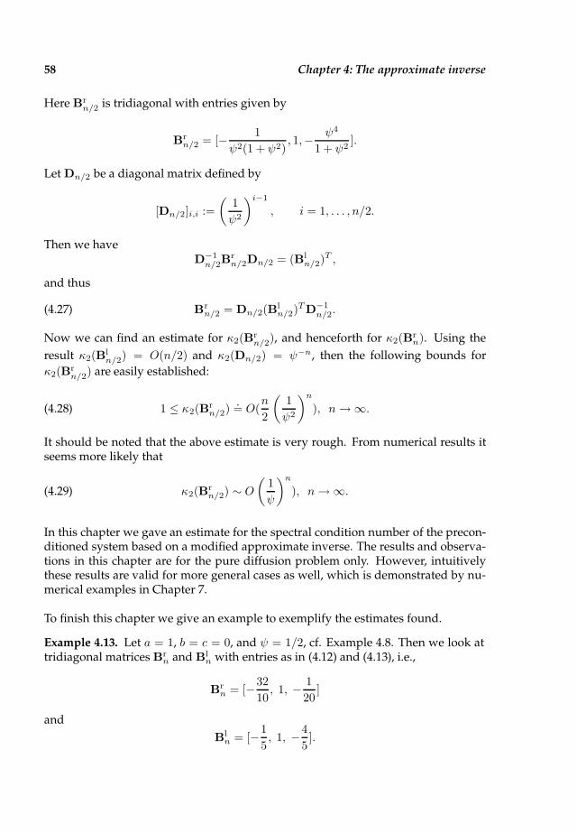
58 Chapter 4: The approximate inverse
Here Brn/2 is tridiagonal with entries given by
Brn/2 = [− 1
ψ2(1 + ψ2), 1,− ψ4
1 + ψ2].
Let Dn/2 be a diagonal matrix defined by
[Dn/2]i,i :=
(
1
ψ2
)i−1
, i = 1, . . . , n/2.
Then we haveD−1n/2B
rn/2Dn/2 = (Bl
n/2)T ,
and thus
(4.27) Brn/2 = Dn/2(B
ln/2)
TD−1n/2.
Now we can find an estimate for κ2(Brn/2), and henceforth for κ2(B
rn). Using the
result κ2(Bln/2) = O(n/2) and κ2(Dn/2) = ψ−n, then the following bounds for
κ2(Brn/2) are easily established:
(4.28) 1 ≤ κ2(Brn/2)
.= O(
n
2
(
1
ψ2
)n
), n→ ∞.
It should be noted that the above estimate is very rough. From numerical results itseems more likely that
(4.29) κ2(Brn/2) ∼ O
(
1
ψ
)n
), n→ ∞.
In this chapter we gave an estimate for the spectral condition number of the precon-ditioned system based on a modified approximate inverse. The results and observa-tions in this chapter are for the pure diffusion problem only. However, intuitivelythese results are valid for more general cases as well, which is demonstrated by nu-merical examples in Chapter 7.
To finish this chapter we give an example to exemplify the estimates found.
Example 4.13. Let a = 1, b = c = 0, and ψ = 1/2, cf. Example 4.8. Then we look attridiagonal matrices Br
n and Bln with entries as in (4.12) and (4.13), i.e.,
Brn = [−32
10, 1, − 1
20]
and
Bln = [−1
5, 1, −4
5].
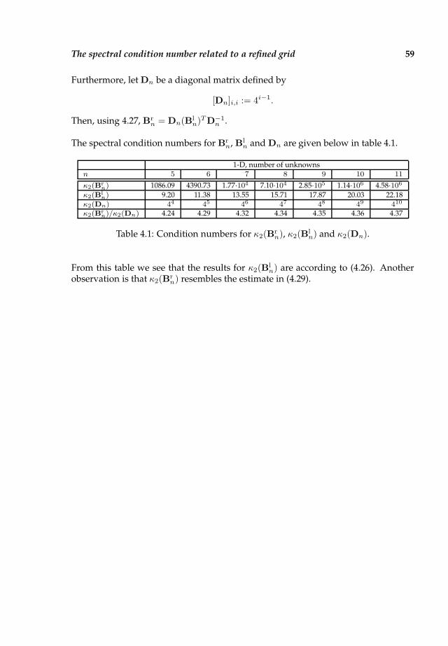
The spectral condition number related to a refined grid 59
Furthermore, let Dn be a diagonal matrix defined by
[Dn]i,i := 4i−1.
Then, using 4.27, Brn = Dn(B
ln)TD−1
n .
The spectral condition numbers for Brn, Bl
n and Dn are given below in table 4.1.
1-D, number of unknownsn 5 6 7 8 9 10 11
κ2(Brn) 1086.09 4390.73 1.77·104 7.10·104 2.85·105 1.14·106 4.58·106
κ2(Bln) 9.20 11.38 13.55 15.71 17.87 20.03 22.18
κ2(Dn) 44 45 46 47 48 49 410
κ2(Brn)/κ2(Dn) 4.24 4.29 4.32 4.34 4.35 4.36 4.37
Table 4.1: Condition numbers for κ2(Brn), κ2(B
ln) and κ2(Dn).
From this table we see that the results for κ2(Bln) are according to (4.26). Another
observation is that κ2(Brn) resembles the estimate in (4.29).

Chapter 5
Recursive solution methods
In this chapter we examine the application of the approximate inverse precondi-tioner for convection diffusion problems as introduced in Chapter 4. In particularwe look at the decoupling mentioned in Example 4.8 and (4.24) in more detail.
In the first part of this chapter we consider a one dimensional setting. Using char-acteristics of the approximate inverse Gn, we show that the preconditioned linearoperator AnGn decouples into two submatrices. On the resulting subproblems,the same decoupling can be obtained using the approximate inverse preconditioneragain. This repeated decoupling gives rise to a recursive solution algorithm. Thecomputational complexity of this algorithm is shown to be O(n log(n)) with n thenumber of degrees of freedom on the finest grid.
Secondly we examine the approximate inverses in two dimensions. Though the con-struction of the approximate inverse Gn is similar to the 1-D case, the final result issomewhat different. The main difference is that the decoupling depends on the typeof operator, as well as on the grid topology (tensor grid, grid of triangles etc.). Fora discretization of the Laplace operator on a uniform grid an interesting observationis made. Even if there is no repeated decoupling, repeated application of approxi-mate inverses seems to lead to approximations of the Laplace operator with a largersupport.
5.1 Decoupling in one dimension
Consider problem (3.1). We discretize this by a finite element method with linear ba-sis functions, or a finite difference method resulting in a three point finite differencestencil. The corresponding n× n matrix An is tridiagonal.
Let S denote the sparsity pattern of An (cf. Section 3.5), i.e.,
(5.1) S := (i, j) : [An]i,j 6= 0.
Because An is symmetric, (i, j) ∈ S implies (j, i) ∈ S. The sparsity pattern of A2n,
denoted by S2, is then given by
(5.2) S2 = (i, j) : ∃k : (i, k) ∈ S ∧ (j, k) ∈ S.
62 Chapter 5: Recursive solution methods
This is easily seen since [A2n]i,j =
∑
k aikakj and the observation that aikakj is non-zero only if i − 2 ≤ j ≤ i + 2. Since the approximate inverse Gn is constructedwith sparsity pattern S, the sparsity pattern of AnGn, say S , will be a subset of S2.Because AnGn satisfies
(5.3) [AnGn]i,j = δi,j for (i, j) ∈ S,we have
S = (i, j) : j = i− 2 ∨ j = i+ 2 ∨ j = i, 1 ≤ j ≤ n.From this we see that the set 1, . . . , n decouples into sets S1 and S2 defined by
S1 = i : i = 2k + 1, 0 ≤ k ≤ d n2e
andS2 = i : i = 2k, 1 ≤ k ≤ bn
2c.
We summarize this in the following.
Property 5.1. For An and Gn as defined above the matrix AnGn is reducible. This impliesthere exist S1 and S2, such that
S = S1 ∪ S2, and S1 ∩ S2 = ∅,that are given by
S1 = (i, j) : i ∈ S1 ∧ [AnGn]i,j 6= 0,and
S2 = (i, j) : i ∈ S2 ∧ [AnGn]i,j 6= 0.2
The result in Property 5.1 can easily be extended to the p-approximate inverse pre-conditioner. Let Sp denote the sparsity pattern of Ap
n, i.e.,
Sp := (i, j) : ∃k1, . . . , kp−1 : (i, k1) ∈ S ∧ (k1, k2) ∈ S ∧ . . . ∧ (kp−1, j) ∈ S,or in term of the band-width
Sp := (i, j) : i− p ≤ j ≤ j = i+ p, 1 ≤ j ≤ n.Since
(5.4) [AnGn]i,j = δi,j for (i, j) ∈ Sp,
we have
Sp = (i, j) : j = i− p− 1 ∨ j = i+ p+ 1 ∨ j = i, 1 ≤ j ≤ n.From this we see that 1, . . . , n decouples into p+ 1 disjoint sets:
Sq = i : k(p+ 1) + q, 0 ≤ k ≤ dnpe, q = 1, . . . , p+ 1.
So, Property 5.1 can be generalized as
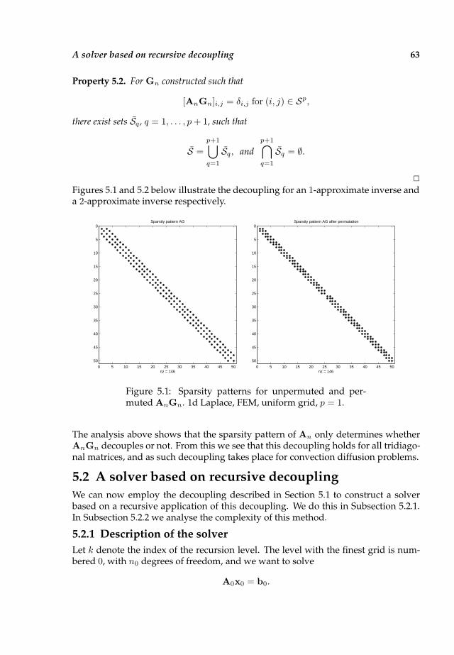
A solver based on recursive decoupling 63
Property 5.2. For Gn constructed such that
[AnGn]i,j = δi,j for (i, j) ∈ Sp,
there exist sets Sq , q = 1, . . . , p+ 1, such that
S =
p+1⋃
q=1
Sq, and
p+1⋂
q=1
Sq = ∅.
2
Figures 5.1 and 5.2 below illustrate the decoupling for an 1-approximate inverse anda 2-approximate inverse respectively.
0 5 10 15 20 25 30 35 40 45 50
0
5
10
15
20
25
30
35
40
45
50
nz = 146
Sparsity pattern AG
0 5 10 15 20 25 30 35 40 45 50
0
5
10
15
20
25
30
35
40
45
50
nz = 146
Sparsity pattern AG after permutation
Figure 5.1: Sparsity patterns for unpermuted and per-muted AnGn. 1d Laplace, FEM, uniform grid, p = 1.
The analysis above shows that the sparsity pattern of An only determines whetherAnGn decouples or not. From this we see that this decoupling holds for all tridiago-nal matrices, and as such decoupling takes place for convection diffusion problems.
5.2 A solver based on recursive decoupling
We can now employ the decoupling described in Section 5.1 to construct a solverbased on a recursive application of this decoupling. We do this in Subsection 5.2.1.In Subsection 5.2.2 we analyse the complexity of this method.
5.2.1 Description of the solver
Let k denote the index of the recursion level. The level with the finest grid is num-bered 0, with n0 degrees of freedom, and we want to solve
A0x0 = b0.
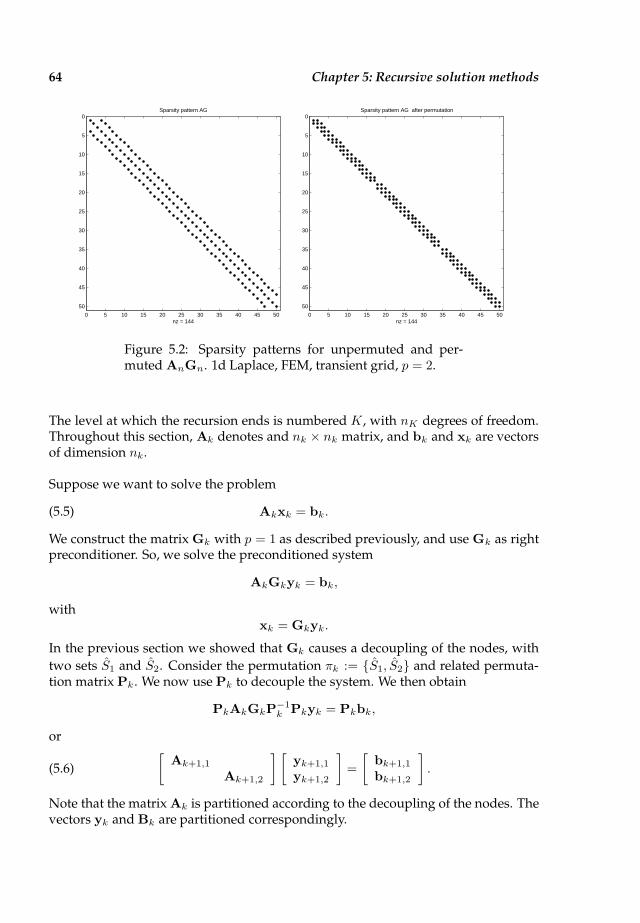
64 Chapter 5: Recursive solution methods
0 5 10 15 20 25 30 35 40 45 50
0
5
10
15
20
25
30
35
40
45
50
nz = 144
Sparsity pattern AG
0 5 10 15 20 25 30 35 40 45 50
0
5
10
15
20
25
30
35
40
45
50
nz = 144
Sparsity pattern AG after permutation
Figure 5.2: Sparsity patterns for unpermuted and per-muted AnGn. 1d Laplace, FEM, transient grid, p = 2.
The level at which the recursion ends is numbered K, with nK degrees of freedom.Throughout this section, Ak denotes and nk × nk matrix, and bk and xk are vectorsof dimension nk.
Suppose we want to solve the problem
(5.5) Akxk = bk.
We construct the matrix Gk with p = 1 as described previously, and use Gk as rightpreconditioner. So, we solve the preconditioned system
AkGkyk = bk,
withxk = Gkyk.
In the previous section we showed that Gk causes a decoupling of the nodes, with
two sets S1 and S2. Consider the permutation πk := S1, S2 and related permuta-tion matrix Pk . We now use Pk to decouple the system. We then obtain
PkAkGkP−1k Pkyk = Pkbk,
or
(5.6)
[
Ak+1,1
Ak+1,2
] [
yk+1,1
yk+1,2
]
=
[
bk+1,1
bk+1,2
]
.
Note that the matrix Ak is partitioned according to the decoupling of the nodes. Thevectors yk and Bk are partitioned correspondingly.
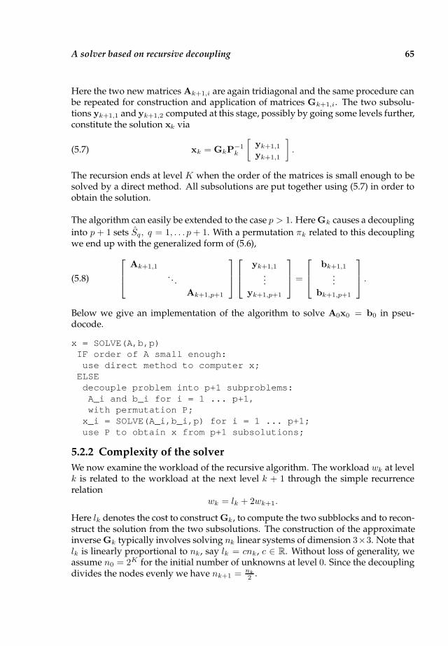
A solver based on recursive decoupling 65
Here the two new matrices Ak+1,i are again tridiagonal and the same procedure canbe repeated for construction and application of matrices Gk+1,i. The two subsolu-tions yk+1,1 and yk+1,2 computed at this stage, possibly by going some levels further,constitute the solution xk via
(5.7) xk = GkP−1k
[
yk+1,1
yk+1,1
]
.
The recursion ends at level K when the order of the matrices is small enough to besolved by a direct method. All subsolutions are put together using (5.7) in order toobtain the solution.
The algorithm can easily be extended to the case p > 1. Here Gk causes a decoupling
into p+ 1 sets Sq, q = 1, . . . p+ 1. With a permutation πk related to this decouplingwe end up with the generalized form of (5.6),
(5.8)
Ak+1,1
. . .
Ak+1,p+1
yk+1,1
...yk+1,p+1
=
bk+1,1
...bk+1,p+1
.
Below we give an implementation of the algorithm to solve A0x0 = b0 in pseu-docode.
x = SOLVE(A,b,p)IF order of A small enough:use direct method to computer x;
ELSEdecouple problem into p+1 subproblems:A_i and b_i for i = 1 ... p+1,with permutation P;
x_i = SOLVE(A_i,b_i,p) for i = 1 ... p+1;use P to obtain x from p+1 subsolutions;
5.2.2 Complexity of the solver
We now examine the workload of the recursive algorithm. The workload wk at levelk is related to the workload at the next level k + 1 through the simple recurrencerelation
wk = lk + 2wk+1.
Here lk denotes the cost to construct Gk, to compute the two subblocks and to recon-struct the solution from the two subsolutions. The construction of the approximateinverse Gk typically involves solving nk linear systems of dimension 3×3. Note thatlk is linearly proportional to nk, say lk = cnk, c ∈ R. Without loss of generality, weassume n0 = 2K for the initial number of unknowns at level 0. Since the decouplingdivides the nodes evenly we have nk+1 = nk
2 .

66 Chapter 5: Recursive solution methods
So the recurrence relation becomes wk = c2K−k + 2wk+1. For the workload at thelowest level K we assume wK = F . The solution is found to be
(5.9) wk =c
2(K − k)2K−k + F2K−k.
This shows that for solving A0x0 = b0 w0 = O(n0 log(n0)). Henceforth this algo-rithm is not optimal. However, there are several issues that can be exploited in orderto improve the workload of the algorithm.Note that nk small subproblems need to be solved for the construction of Gk. If thisis done in parallel the factor lk will no longer be linearly proportional to nk and wemay assume lk = c. Then (5.9) becomes wk = (F + c)2K−k − c, which is of the orderO(nk).Another remark is that similarity of the subsystems can be used to reduce computa-tional cost. For a stiffness matrix related to a uniform grid for instance, the relatednk subsystems that need to be solved to obtain Gk come in three types only: one foreach boundary, and one for all interior points. This implies that only a few subsys-tems actually need to be solved, and hence the factor lk will be O(1).
For this generalized version where p > 1 it is easily seen that the workload wk atlevel k is estimated by
(5.10) wk = lk + (p+ 1)wk+1.
Here lk denotes the effort to compute Gk, obtain the decoupling, and reconstructthe solution. Construction of Gk involves solving Nk linear systems of dimension(2p + 1) × (2p + 1). If p is large, computation of the local Green’s functions gi isexpensive. Also storage requirements for Gk increase with increasing p. However,a larger p may be beneficial since the criteria on when to solve the subsystems by adirect method is reached in fewer steps.
5.3 Decoupling in two dimensions
Consider now problem (3.1) in two dimension with b = 0 and c = 0. Let us coverthe domain Ω with a uniform grid, with m degrees of freedom in both directions, son = m2. A finite difference discretization, or a finite element discretization results inthe linear system of equations
(5.11) Anxn = bn.
As in Section 5.1, let S denote the sparsity pattern of An
(5.12) S := (i, j) : [An]i,j 6= 0.
Because of symmetry we have
(i, j) ∈ S ⇐⇒ (j, i) ∈ S.
In the next lemma we look at the sparsity pattern S2 of A2n and how it relates to S.

Decoupling in two dimensions 67
Property 5.3. Let S2 denote the sparsity pattern of A2n. Then we have
S2 := (i, j) : ∃k : (i, k) ∈ S ∧ (j, k) ∈ S.Proof. Let l be a number such that (i, l) ∈ S and (j, l) ∈ S for some i and j. Becauseof symmetry we also have (l, j) ∈ S and it follows that ailalj 6= 0. Entry [A2
n]i,j isdefined by
∑
k aikakj . Since for k = l we have a non-zero contribution to this sum,the pair (i, j) related to entry [A2]i,j is contained in the sparsity pattern.
This means that the sparsity pattern of A2n is the sparsity pattern of An comple-
mented by the ” neighbours’ neighbours“: If there are numbers i, j, k such that (i, j) ∈S, (j, k) ∈ S and (i, k) 6∈ S, then (i, k) ∈ S2. Since this statement on the sparsitypattern of A2
n holds for any two different matrices with identical sparsity patterns, itis also true for AnGn with the extra knowledge that for some (i, j) ∈ S2 it holds that[AnGn]i,j = 0. This is because of the property
[AnGn]i,j = δi,j for (i, j) ∈ S.Then the sparsity pattern S of AnGn can be defined as
S := (i, j) : ∃k, k 6= i : (i, k) ∈ S ∧ (j, k) ∈ S ∧ [AnGn]i,k = [AnGn]j,k = 0.So, a degree of freedom i gets disconnected from its neighbours, but becomes con-nected to the neighbour’s neighbours, as shown in figure 5.3 for a uniform grid. Aneighbour is no longer a neighbour after the right multiplication by Gn. The leftpicture in figure 5.3 is correct for a FDM discretization of −a∆u+b ·∇u+ cu, as wellfor a FEM discretization of −a∆u+ cu.
Initial coupling of central dof New coupling of central dof
Figure 5.3: Initial connectivity in An and new connectivity in AnGn.
Next we examine whether there is a decoupling of the degrees of freedom as seen inthe one dimensional case. We have a uniform grid with m nodes in both directions,and we number the points from 1 to m2 from bottom to top and from left to right.For node i let Si denote the set of nodes that are neighbours of i, i.e.,
Si = i+ 1, i+m, i− 1, i−m,
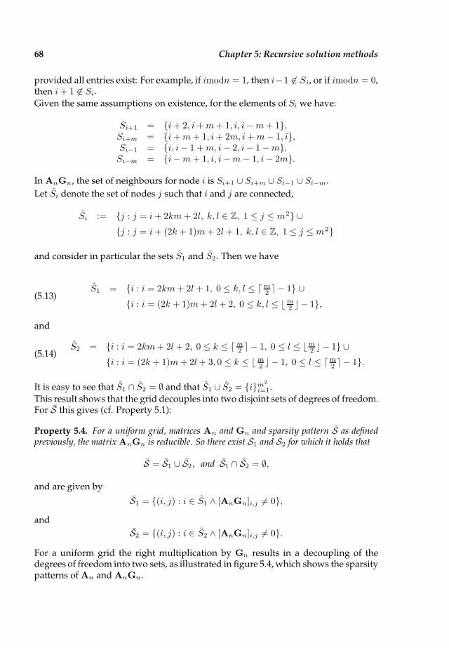
68 Chapter 5: Recursive solution methods
provided all entries exist: For example, if imodn = 1, then i−1 6∈ Si, or if imodn = 0,then i+ 1 6∈ Si.
Given the same assumptions on existence, for the elements of Si we have:
Si+1 = i+ 2, i+m+ 1, i, i−m+ 1,Si+m = i+m+ 1, i+ 2m, i+m− 1, i,Si−1 = i, i− 1 +m, i− 2, i− 1 −m,Si−m = i−m+ 1, i, i−m− 1, i− 2m.
In AnGn, the set of neighbours for node i is Si+1 ∪ Si+m ∪ Si−1 ∪ Si−m.
Let Si denote the set of nodes j such that i and j are connected,
Si := j : j = i+ 2km+ 2l, k, l ∈ Z, 1 ≤ j ≤ m2 ∪j : j = i+ (2k + 1)m+ 2l + 1, k, l ∈ Z, 1 ≤ j ≤ m2
and consider in particular the sets S1 and S2. Then we have
(5.13)S1 = i : i = 2km+ 2l + 1, 0 ≤ k, l ≤ dm2 e − 1 ∪
i : i = (2k + 1)m+ 2l+ 2, 0 ≤ k, l ≤ bm2 c − 1,
and
(5.14)S2 = i : i = 2km+ 2l + 2, 0 ≤ k ≤ dm2 e − 1, 0 ≤ l ≤ bm2 c − 1 ∪
i : i = (2k + 1)m+ 2l+ 3, 0 ≤ k ≤ bm2 c − 1, 0 ≤ l ≤ dm2 e − 1.
It is easy to see that S1 ∩ S2 = ∅ and that S1 ∪ S2 = im2
i=1.
This result shows that the grid decouples into two disjoint sets of degrees of freedom.For S this gives (cf. Property 5.1):
Property 5.4. For a uniform grid, matrices An and Gn and sparsity pattern S as definedpreviously, the matrix AnGn is reducible. So there exist S1 and S2 for which it holds that
S = S1 ∪ S2, and S1 ∩ S2 = ∅,
and are given by
S1 = (i, j) : i ∈ S1 ∧ [AnGn]i,j 6= 0,
and
S2 = (i, j) : i ∈ S2 ∧ [AnGn]i,j 6= 0.
For a uniform grid the right multiplication by Gn results in a decoupling of thedegrees of freedom into two sets, as illustrated in figure 5.4, which shows the sparsitypatterns of An and AnGn.

Decoupling in two dimensions 69
0 5 10 15 20 25 30 35 40 45 50
0
5
10
15
20
25
30
35
40
45
50
Sparsity pattern A
0 5 10 15 20 25 30 35 40 45 50
0
5
10
15
20
25
30
35
40
45
50
Sparsity pattern AG
0 5 10 15 20 25 30 35 40 45 50
0
5
10
15
20
25
30
35
40
45
50
Sparsity pattern AG after permutation
Figure 5.4: Sparsity patterns for An, AnGn, and AnGn after permutation.
Remark 5.5. A consequence of the above property is that the matrix AnGn decou-ples into two matrices, say B1 and B2. Now it is interesting to see that the rows ofthese matrices satisfy the stencil
[− 1
12, −1
6, −1
6, − 1
12, 1, − 1
12, −1
6, −1
6, − 1
12].
This stencil corresponds to a nine point finite difference approximation for the Laplaceoperator given by
∇2u(x, y).=
1
8(
1
h2(u(x, y) − 1
12u(x, y − 2h) − 1
6u(x− h, y − h)−
1
6u(x+ h, y − h) − 1
12u(x− 2h, y) − 1
12u(x+ 2h, y)−
1
6u(x− h, y + h) − 1
6u(x+ h, y + h) − 1
12u(x, y + 2h)).
So far we have considered only matrices Gn that inherit the sparsity pattern of An. Insection 5.1 construction of Gn was examined where the sparsity pattern of Ap
n, p > 1was used as a template. So, let Sp denote the sparsity pattern of Ap
n,
(5.15) Sp = (i, j) : ∃k1, . . . kp−1 : (i, k1) ∈ S ∧ (k1, k2) ∈ S ∧ . . . ∧ (kp−1, j) ∈ S,
and let Gn be such that (5.4) is satisfied. Let Sp denote the sparsity pattern of AnGn.For p = 1 we showed that S decouples into two disjoint sets. However for p = 2there is no decoupling. In order to see this, we show that a node i remains connectedto its neighbours. Let
(5.16) Si = i ∪ i+ am+ b : −3 ≤ a, b ≤ 3, |a| + |b| = 3.
For i + 2m + 1 in this set, we take a closer look at Si+2m+1. We see i + m + 3 ∈Si+2m+1, and for Si+m+3 we find i + 1 ∈ Si+m+3. So, we have (i, i + 2m + 1) ∈ S2,(i + 2m + 1, i + m + 3) ∈ S2 and (i + m + 3, i + 1) ∈ S2. From this it follows that(i, i + 1) ∈ S2. Similarly we can show that i is connected to its other neighbours aswell.
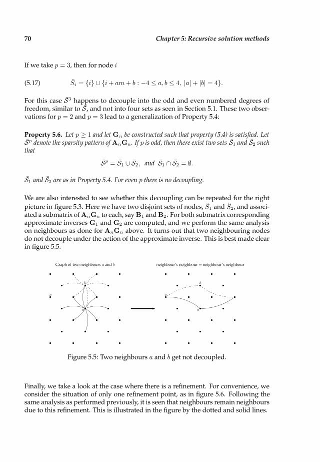
70 Chapter 5: Recursive solution methods
If we take p = 3, then for node i
(5.17) Si = i ∪ i+ am+ b : −4 ≤ a, b ≤ 4, |a| + |b| = 4.
For this case S3 happens to decouple into the odd and even numbered degrees offreedom, similar to S , and not into four sets as seen in Section 5.1. These two obser-vations for p = 2 and p = 3 lead to a generalization of Property 5.4:
Property 5.6. Let p ≥ 1 and let Gn be constructed such that property (5.4) is satisfied. LetSp denote the sparsity pattern of AnGn. If p is odd, then there exist two sets S1 and S2 suchthat
Sp = S1 ∪ S2, and S1 ∩ S2 = ∅.
S1 and S2 are as in Property 5.4. For even p there is no decoupling.
We are also interested to see whether this decoupling can be repeated for the right
picture in figure 5.3. Here we have two disjoint sets of nodes, S1 and S2, and associ-ated a submatrix of AnGn to each, say B1 and B2. For both submatrix correspondingapproximate inverses G1 and G2 are computed, and we perform the same analysison neighbours as done for AnGn above. It turns out that two neighbouring nodesdo not decouple under the action of the approximate inverse. This is best made clearin figure 5.5.
Graph of two neighbours a and b
a
b
c
neighbour’s neighbour = neighbour’s neighbour
a
b
c
Figure 5.5: Two neighbours a and b get not decoupled.
Finally, we take a look at the case where there is a refinement. For convenience, weconsider the situation of only one refinement point, as in figure 5.6. Following thesame analysis as performed previously, it is seen that neighbours remain neighboursdue to this refinement. This is illustrated in the figure by the dotted and solid lines.
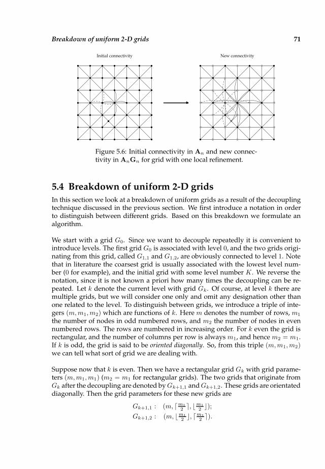
Breakdown of uniform 2-D grids 71
Initial connectivity New connectivity
Figure 5.6: Initial connectivity in An and new connec-tivity in AnGn for grid with one local refinement.
5.4 Breakdown of uniform 2-D grids
In this section we look at a breakdown of uniform grids as a result of the decouplingtechnique discussed in the previous section. We first introduce a notation in orderto distinguish between different grids. Based on this breakdown we formulate analgorithm.
We start with a grid G0. Since we want to decouple repeatedly it is convenient tointroduce levels. The first grid G0 is associated with level 0, and the two grids origi-nating from this grid, called G1,1 and G1,2, are obviously connected to level 1. Notethat in literature the coarsest grid is usually associated with the lowest level num-ber (0 for example), and the initial grid with some level number K. We reverse thenotation, since it is not known a priori how many times the decoupling can be re-peated. Let k denote the current level with grid Gk. Of course, at level k there aremultiple grids, but we will consider one only and omit any designation other thanone related to the level. To distinguish between grids, we introduce a triple of inte-gers (m,m1,m2) which are functions of k. Here m denotes the number of rows, m1
the number of nodes in odd numbered rows, and m2 the number of nodes in evennumbered rows. The rows are numbered in increasing order. For k even the grid isrectangular, and the number of columns per row is always m1, and hence m2 = m1.If k is odd, the grid is said to be oriented diagonally. So, from this triple (m,m1,m2)we can tell what sort of grid we are dealing with.
Suppose now that k is even. Then we have a rectangular grid Gk with grid parame-ters (m,m1,m1) (m2 = m1 for rectangular grids). The two grids that originate fromGk after the decoupling are denoted byGk+1,1 andGk+1,2. These grids are orientateddiagonally. Then the grid parameters for these new grids are
Gk+1,1 : (m, dm1
2 e, bm1
2 c);Gk+1,2 : (m, bm1
2 c, dm1
2 e).

72 Chapter 5: Recursive solution methods
For odd k, we have a diagonally orientated grid Gk with parameters (m,m1,m2).The grids Gk+1,1 and Gk+1,2 resulting from the decoupling are rectangular and haveparameters as follows
Gk+1,1 : (dm2 e,m1,m1);
Gk+1,2 : (bm2 c,m2,m2).
Table 5.1 shows the grids that originate from an initial 7× 7 grid, represented by thetriple (m,m1,m2). In figures 5.7 and 5.8 the decoupling is made visible by depictingthe nodes of the initial grid and its two successors.
k = 0 (7, 7, 7)k = 1 (7, 4, 3) (7, 3, 4)k = 2 (4, 4, 4) (3, 3, 3) (4, 3, 3) (3, 4, 4)k = 3 (4, 2, 2) (4, 2, 2) (3, 2, 1) (3, 1, 2) (4, 2, 1) (4, 1, 2) (3, 2, 2) (3, 2, 2)
Table 5.1: Breakdown of a 7× 7 grid after three decomposi-tions, grid parameters are (m,m1,m2) shown.
Grid Grid Grid
Figure 5.7: Decomposition of the rectangular (7, 7, 7) gridinto two diagonally oriented sets of nodes.
Grid Grid Grid
Figure 5.8: Decomposition of the diagonal (7, 4, 3) grid intotwo rectangularly oriented sets of nodes.
Related to grid Gk is the stiffness matrix Ak based on a finite element of finite differ-ence discretization on that grid. The stiffness matrices related to the grid Gk+1,1 and

Three algorithms based on forced repeated decoupling 73
Gk+1,2 are denoted by Ak+1,1 and Ak+1,2 respectively. The order nk of a stiffnessmatrix Ak related to a grid Gk with parameters (m,m1,m2) are easily found to be
k even : m ·m1;
k odd : dm2 em1 + bm2 cm2.
Now we have Ak and Gk we find that the new matrix AkGk decouples into partsAk+1,1 and Ak+1,2.
5.5 Three algorithms based on forced repeated decou-
pling
In the previous section we introduced definitions for grids, and explained how twonew grids Gk+1,1 and Gk+1,2 originate from initial grid Gk. This creation of twonew grids implies a decoupling of the original degrees of freedom into two disjointsets. With a proper permutation based on this decoupling the related linear operatorAkGk can be written as a 2 × 2 block matrix.
At level k we have to solve the system of equations
(5.18) Akxk = bk.
We construct the Green’s matrix Gk. Next, Gk is applied as a right preconditioner,and we solve
AkGkyk = bk,
with
(5.19) xk = Gkyk.
The multiplication of Ak by the Green’s matrix Gk results in a decoupling of the
degrees of freedom into two disjoint sequences S1 and S2. Consider the permutation
πk := (S1 S2) and the corresponding permutation matrix Pk The permutation ofvariables reorders the degrees of freedom such that the two sets are numbered oneafter each other. We apply this permutation in order to get the decoupled system.This is the linear system
(5.20) PkAkGkPTkPkyk = Pkbk.
Note that PTk = P−1
k . This system is a 2 × 2 block system where all sub blocks are oflevel k + 1:
(5.21)
[
Ak+1,1
Ak+1,2
] [
yk+1,1
yk+1,2
]
=
[
bk+1,1
bk+1,2
]
.
Here[
Ak+1,1
Ak+1,2
]
:= PkAkGkPTk ,
74 Chapter 5: Recursive solution methods
[
yk+1,1
yk+1,2
]
:= Pkyk
and[
bk+1,1
bk+1,2
]
:= Pkbk.
There are two independent linear subsystems,
(5.22)
Ak+1,1yk+1,1 = bk+1,1,
Ak+1,2yk+1,2 = bk+1,2,
to be solved, instead of one system in (5.18). These are related to two sub grids ofGk , called Gk+1,1 and Gk+1,2 respectively. At this new level k + 1 the decouplingprocedure is to be repeated. Unfortunately this cannot be accomplished with thematrices Ak+1,i, i = 1, 2, as outlined in the previous section. However, given theregularity of the new grids Gk+1,1 and Gk+1,2 it is possible to repeat the decoupling.In the following three algorithms are presented that make use of this.
5.5.1 A recursive preconditioner: I
A first idea is to find suitable preconditioners for the two linear systems in (5.22).Related to grids Gk+1,1 andGk+1,2 we construct Laplace matrices Ak+1,1 and Ak+1,2
such that these matrices can be decoupled using Green’s matrices Gk+1,1 and Gk+1,2.So, the Laplace matrices Ak+1,1 and Ak+1,2 are utilized as preconditioners for Ak+1,1
and Ak+1,2 respectively. The next step in the algorithm is to solve the preconditionedsystems
(5.23)
A−1k+1,1Ak+1,1yk+1,1 = A−1
k+1,1bk+1,1
A−1k+1,2Ak+1,2yk+1,2 = A−1
k+1,2bk+1,2.
Both Ak+1 and Ak+1 are discretizations of the Laplace operator: Ak+1 is related tothe a five point discretization, and Ak+1 to a nine point discretization. So, since Ak+1
and Ak+1 are discretizations of the same operator, it makes sense to use one of thetwo as preconditioner for the other. Furthermore, we have seen that the matrix Ak+1
related to the five point stencil decouples after multiplication with the correspondingGreen’s matrix Gk+1.In iterative methods systems of equations with Ak+1,1 and Ak+1,2 have to be solvedin order to apply this preconditioner. In order to solve these systems, the same pro-cess of computing Green’s matrices Gk+1,1 and Gk+1,2, and decoupling of the thedegrees of freedom is repeated. The two subsolutions yk+1,1 and yk+1,2 are com-puted at this stage, possibly by going some levels further. Using (5.19) the solutionxk is obtained via
(5.24) xk = GkP−1k
[
yk+1,1
yk+1,2
]
.
The recursion terminates at level K > 0 when the dimensions of the linear systemsAK at that level are such that the systems of equations can be solved using a direct
Three algorithms based on forced repeated decoupling 75
method. The 2K partial solutions are assembled to obtain the solution of the originalproblem A0x0 = b0.
Below we give an implementation of the algorithm described above in (5.18) - (5.24),called SOLVE-I, by the following pseudocode:
x = SOLVE-I(A, rhs)IF order of A small enough:use direct method to compute x;
ELSEsplit A into two subproblems:A1p, rhs1 and preconditioner A1,A2p, rhs2 and preconditioner A2,with permutation P;
x1 = CGS(A1p, rhs1, SOLVE-I(A1), EPS, MAXIT);x2 = CGS(A2p, rhs2, SOLVE-I(A2), EPS, MAXIT);use permutation P to obtain x from x1 and x2;
END
The tolerance EPS and maximum number of iterations MAXIT used by the inner CGSiterative method are shown explicitly since these two parameters influence speedand accuracy of SOLVE-I.
There are two ways to use the SOLVE-I algorithm: directly as a solver, or as a pre-conditioner. When used as a solver, the call is directly to the algorithm:
x = SOLVE-I(A, rhs).
When used as a preconditioner inside an iterative method, the use of SOLVE-I is asfollows:
x = CGS(A, rhs, SOLVE-I, EPS, MAXIT).
5.5.2 A recursive preconditioner: II
In the SOLVE-I algorithm in the previous subsection the recursive nature followsfrom (5.23). Since both Ak+1,i and Ak+1,i are matrices related to different discretiza-tions of the Laplace operator, we consider substitution of Ak+1,i by Ak+1,i. Withthis approach, matrices Ak+1,i need not to be computed explicitly. Another benefitis that Ak+1,i required less storage since these matrices are sparser.So, the linear systems in (5.23) with Ak+1,i are replaced by Ak+1,i resulting in
(5.25)
Ak+1,1yk+1,1 = bk+1,1,Ak+1,2yk+1,2 = bk+1,2,
In this alternative in the recursive step we solve
Ak+1yk+1 = bk+1
76 Chapter 5: Recursive solution methods
instead of
Ak+1yk+1 = bk+1.
An updated version of the algorithm, now called SOLVE-II reads as follows:
x = SOLVE-II(A, rhs)IF order of A small enough:use direct method to compute x;
ELSEsplit A into two subproblems:A1 and rhs1,A2 and rhs2,with permutation P;
x1 = CGS(A1, rhs1, SOLVE-II(A1), EPS, MAXIT);x2 = CGS(A2, rhs2, SOLVE-II(A2), EPS, MAXIT);use permutation P to obtain x from x1 and x2;
END
5.5.3 A recursive preconditioner: III
The above algorithm can be altered even further, by simply replacing the calls toan iterative method by a call to the algorithm itself. This results in the followingalgorithm:
x = SOLVE-III(A, rhs)IF size of A small enough:
use direct method to compute x;ELSE
construct two matrices related to splitting of A:A1 and rhs1,A2 and rhs2,
with permutation P;x1 = SOLVE-III(A1, rhs1);x2 = SOLVE-III(A2, rhs2);use permutation P to obtain x from x1 and x2;
END
To summarize, we have three versions of the SOLVE algorithm:
1. [SOLVE-I] The algorithm with inner iterative solvers to solveA−1k+1Ak+1yk+1 = A−1
k+1bk+1;
2. [SOLVE-II] The algorithm with inner iterative solvers to solveAk+1yk+1 = bk+1;
3. [SOLVE-III] The algorithm with a recursive call to itself.
Complexity of the algorithms 77
5.6 Complexity of the algorithms
The work at level k to solve the system Akxk = bk depends on the tolerance ε (EPSin the SOLVE algorithms in Section 5.5) and is denoted by wk(ε). The work at thislevel, except for the work required to solve the two subproblems, is denoted by lk.This involves construction of the Green’s matrix and the related permutation. Thework required by the iterative method used (CGS for example) is denoted by gk.Finally, let λk(ε) denote the average number of iterations needed for solving the twosubproblems. Then we obtain the following estimate for level k,
(5.26) wk(ε) = lk + 2λk+1(ε)(gk+1 + wk+1(ε)).
For CGS we assume λ(ε) iterations. Apart from wk+1(ε) as indicated above eachiteration costs 18nk+1 flops, see [9]. Furthermore, lk = 3nk (approximation for thework to obtain the permutation, but still linear in the amount of degrees of freedom).We assume nk+1 = nk
2 , and henceforth nk = 2K−knK where nK denotes the amountof degrees of freedom at level K when a direct method is used. The work at level Kis fixed: wK(ε) = wK .
Then the workload wk(ε) at level k is expressed as follows:
wk(ε) = awk+1(ε) + bnK2K−k.
Here
a = 2λ(ε),
b = 3 + 18λ(ε).
We can solve this recursion:
wk(ε) = aK−kwK + bnK2K−k (a2 )K−k − 1a2 − 1
.
Whence for the total workload w0(ε) to solve A0x0 = b0 we have
(5.27) w0(ε).= O(λ(ε)K(wK + n0)).

Chapter 6
NumLab concepts
The scientific computing numerical and visualization algorithms are becoming moreand more complex. The construction of such algorithms from source code becomesexpensive: Interpretation is too slow, compilation prevents interactive steering andoverview gets lost. To make it worse, there is no formal computer language specifica-tion of complex mathematical notions such as partial differential equations, ordinarydifferential equations, boundary value problems, etc..
With this situation in mind this chapter discusses the concepts of the NumLab com-putational platform. The aim of NumLab is to aid in the rapid (better) software con-struction for complex scientific computations and visualizations. Though softwaremight also be written with the available tools on the market, down to the use of as-sembler code, this would take an insubordinate amount of time. Our goal is to writethe same software much faster and in a convenient manner. To aid the rapid soft-ware development, NumLab offers toolboxes of high level operators and invarianceof important operator properties under operator composition.
First a brief introduction of existing architectures is given, followed by the goals tobe achieved by NumLab.
6.1 Introduction
From a structural point of view, software environments for numerical computationscan be classified into three categories (see for instance [82]): Libraries, turnkey sys-tems, and application frameworks.
Libraries for numerical algorithms such as LAPACK [2], NAGLIB [79], or IMSL [53],or for visualization such as OpenGL [55], Open Inventor [105], or VTK [87], provideservices in the form of data structures and functions. Libraries are usually easy toextend with new data types and functions. However, using libraries to build a com-plete computational or visualization application requires involved programming.
Turnkey systems, such as Matlab [67], Mathematica [107], or the many existing dedi-cated numerical simulators on the market, are simpler to use than libraries to build acomplete application. However, extending the functionality of such systems is usu-ally limited to a given application domain, as in the case of the dedicated simulators,or to a fixed set of supported data types, as in the case of the Matlab programmingenvironment.
80 Chapter 6: NumLab concepts
Application (computational) frameworks, such as the Diffpack and SciLab systems forsolving differential equations [26, 54] or the Oorange system for experimental math-ematics [48] combine the advantages of the libraries and turnkey systems. On onehand, frameworks have an open structure, similar to libraries, so they can be ex-tended with new components, such as solvers, matrix storage schemes, or mesh gen-erators. On the other hand, some frameworks (notably visualization) offer an easymanner to construct a complete application that combines visualization, numericalcomputations, and user interaction. This is usually provided by means of visualprogramming tools such as Matlab’s Simulink [67] or the dataflow network editingtools of the AVS [97], IRIS Explorer [1], or Oorange [48] frameworks. In these frame-works, applications are constructed by assembling visual representations (icons) ofthe computational or visualization components in a network. Program execution isimplemented in terms of computational operations on the network nodes and dataflows between these nodes respectively.
With the above in mind, let us consider how the NumLab environment integratesthe advantages of the above architectures. On the level of libraries, NumLab’s C++routines call Fortran, Pascal, C and C++. Next, similar to a turnkey system, NumLaboffers full integration of visualization and numerical computation and implementscommunication with other environments such as Simulink [67] and MathLink [107].On the application framework level, NumLab provides interactive application con-struction with its visual programming dataflow system Vission [92, 94]. Furthermore,NumLab provides an object-level (subroutine-level) make-concept which allows forinteractive program validification.
In order to better address NumLab’s merits on all levels, we need a closer lookat computational frameworks. Though efficient and effective, most existing com-putational frameworks are limited in several respects. First, limitations exist fromthe perspectives of the end user, application designer, and component developer[3, 37, 82, 94]. First, few computational frameworks facilitate convenient interactionbetween visualization (data exploration) and computations (numerical exploration),both essential to the end user. Secondly, from the application designer’s perspec-tive, the visual programming facility, often provided in visualization frameworkssuch as AVS or Explorer [1, 97], is usually not available for numerical frameworks.Conversely, it is quite difficult to integrate large scale computational libraries in vi-sualization frameworks.
Finally, from the numerical component developer perspective, understanding andextending a framework’s architecture is still (usually) a very complex task, albeitnoticeably simplified in object-oriented environments such as [26, 87].
Next to limitation with respect to the three types of users, many computationalframeworks are constrained in a more structural manner: Similar mathematical con-cepts are not factored out into similar software components. As a consequence, mostexisting numerical software is heterogeneous, thus hard to deploy and understand.For instance, in order to speed up the iterative solution of a system of linear equa-
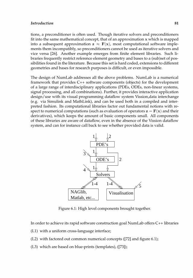
Introduction 81
tions, a preconditioner is often used. Though iterative solvers and preconditionersfit into the same mathematical concept, that of an approximation x which is mappedinto a subsequent approximation z ≈ F(x), most computational software imple-ments them incompatibly, so preconditioners cannot be used as iterative solvers andvice versa [26]. Another example emerges from finite element libraries. Such li-braries frequently restrict reference element geometry and bases to a (sub)set of pos-sibilities found in the literature. Because this set is hard coded, extensions to differentgeometries and bases for research purposes is difficult, or even impossible.
The design of NumLab addresses all the above problems. NumLab is a numericalframework that provides C++ software components (objects) for the developmentof a large range of interdisciplinary applications (PDEs, ODEs, non-linear systems,signal processing, and all combinations). Further, it provides interactive applicationdesign/use with its visual programming dataflow system Vission,data interchange(e.g. via Simulink and MathLink), and can be used both in a compiled and inter-preted fashion. Its computational libraries factor out fundamental notions with re-spect to numerical computations (such as evaluation of operators z = F(x) and theirderivatives), which keeps the amount of basic components small. All componentsof these libraries are aware of dataflow, even in the absence of the Vission dataflowsystem, and can for instance call back to see whether provided data is valid.
Visualisation
Solvers
ODE’s
PDE’s
Matlab, etc...NAGlib,
1-4
2
23
5
1
1
14
1-4
Figure 6.1: High level components brought together.
In order to achieve its rapid software construction goal NumLab offers C++ libraries
(L1) with a uniform cross-language interface;
(L2) with factored out common numerical concepts ([72] and figure 6.1);
(L3) which are based on blue-prints (templates), ([73]);

82 Chapter 6: NumLab concepts
(L4) with high level components (PDE solvers, complex vector field visualizations,see figure 6.1 ([71]));
(L5) which can be used for interpretation ([27]);
(L6) which can all be used for visual programming,
and in addition:
(A1) a visual programming application called Vission ([93]).
There are libraries based on both public and commercial software, and for both sci-entific computing and visualization purposes.The libraries have been designed with other important goals in mind as well, butmost of these are out of the scope of this thesis: parallelism, generation of C++ fromvisual networks and vice versa, Turing completeness. The choice of an existing com-puter language was based on the desire not to add another language to the tower ofBabel – different from the Lawrence Livermore BABEL project which introduces annew scientific interface definition language (SIDL). The choice for C++ was simple:It is a kind of computer language superset.
The properties of the NumLab libraries above ensure:
(M1) abstraction from data representation and much less different manuals to read;
(M2) second opinions (different solver/visualization) at about no cost;
(M3) speed due to on demand generation of specialized code from generic blue-prints;
(M4) composition of complex solvers with just a few components;
(M5) low learning curve (comparable to Matlab);
(M6) overview and convenience.
The Vission application ensures crash-safe operation across multiple libraries ([81]).
The work required for the creation of the NumLab libraries can also be split corre-sponding to the six points as follows:
(W1) encapsulation of all libraries and generation of data-conversion code;
(W2) factorization of concepts across libraries;
(W3) refactorization of libraries and production of in-house written libraries;
(W4) production of in-house written prototype libraries;
(W5) restriction to CINT C++ subset [27];
(W6) restriction to the Vission (C++) concepts [93].
Introduction 83
In practice the restriction to the CINT C++ subset has not lead to restrictions on theencapsuled libraries: In C++ a certain result can be achieved with different algo-rithms (different pieces of code) and so far we have not encountered problems wecould not solve.The restrictions to the concepts of the Vission application were harder to deal withdue to the Vission’s research status. For instance, Vission does not offer naked point-ers as C++ does. This complicates matters: Libraries such as the professional Visu-alization ToolKit VTK libraries could not be encapsuled one to one with the sourcecode, which leads to maintenance problems (each new version of VTK requires athorough inspection). The fact is that it is possible to also introduce naked pointersin Vission, but this would not solve all problems with libraries that return pointers.The encapsulation of public domain and commercial libraries consumes a lot of timebut can, will and is automated for all or part of the task. In fact, most (eliminated)weaknesses in the NumLab libraries have been found in an attempt to automate theencapsulation.
The development of numerical libraries which function ”as expected“ in the visualdata-flow application (A1) consumed a large part of the amount of time dedicatedto the development of the NumLab libraries. The reason is that it was difficult towrite numerical libraries which lived up to the envisioned advantages: The visualrepresentation of a computer program should be a kind of network which shouldoffer:
(N1) structure: a network which contains function/object instances and argumentconnections/alterations;
(N2) structure: data travels from the top of this network (source) and gets altered onits journey down to the bottom (output);
(N3) overview: a network with just a few components can form a complex applica-tion;
(N4) overview: network details can be hidden and be shown on demand;
(N5) interaction: a network accepts graphical input next to the standard console orfile input;
(N6) interaction: while it is executed a network can be altered in order to speed upthe computations.
In order to achieve this, two major problems had to be addressed. First, visualizationof low level components (such as a sorting algorithm) is
1. slow due to the interpretation,
2. and tends to become a visual mess of connections due to the multiple use of adatum.
84 Chapter 6: NumLab concepts
Visualization of all levels of numerical components is further difficult because
3. (iterative) code tends to rebind (x(k) 7→ x(k+1)), for which no standard visualrealization exist,
4. and therefore control loops are non-trivial to realize.
To overcome the low level problems, NumLab as well as VTK/Inventor only of-fers high level visual components such as linear-system solvers, ODE solvers, PDEsolvers, etc.. To overcome the second problem, libraries such as VTK and Inven-tor make the problem the visual application’s problem. For visualization problems,that seems fine, but for numerical problems, where fixed point iterations and henceloops dominate the scene, this is impossible. Hence, NumLab offers primitives forloop control.
This thesis adds both to the NumLab concepts and its content. As part of the work,iterative solution routines and preconditioners were added to NumLab. The con-struction of libraries for the Vission application are commented at in the followingorder. First, Section 6.2 presents the NumLab foundations, which are principles towhich components of NumLab adhere. More in detail, Section 6.3 comments on theNumLab elements and Section 6.4 examines NumLab operators. These are dividedinto the categories systems of equations in Subsection 6.4.1, solvers and preconditionersin Subsection 6.4.2, partial differential equations in Subsection 6.4.3 and ordinary differ-ential equations in Subsection 6.4.4. Next, Section 6.5 explains how NumLab factorsout common components. Details with regard to the implementations are providedin subsections.
6.2 The foundation of NumLab
NumLab offers various elements x of linear vector spaces V and operators F be-tween such spaces. For all elements x,y ∈ V and a scalar c it offers
1. All vectorspace operations: x + y, c · x, etc..
For each operator F, it offers
2. Evaluation: z = F(x) which returns an element.
And for each differentiable operator F and element x, it offers:
3. Jacobian determination: Z = dF(x) which returns a linear operator.
The Jacobian determination can be exact or numerical and should be the Frechetderivative; NumLab cannot examine continuity of the derivative.
The NumLab concept is the simplest possible: For an evaluation z = F(x), each op-erator F can use other elements xii, other elements zii as well as other operatorsFii; for a visual representation see figure 6.2.
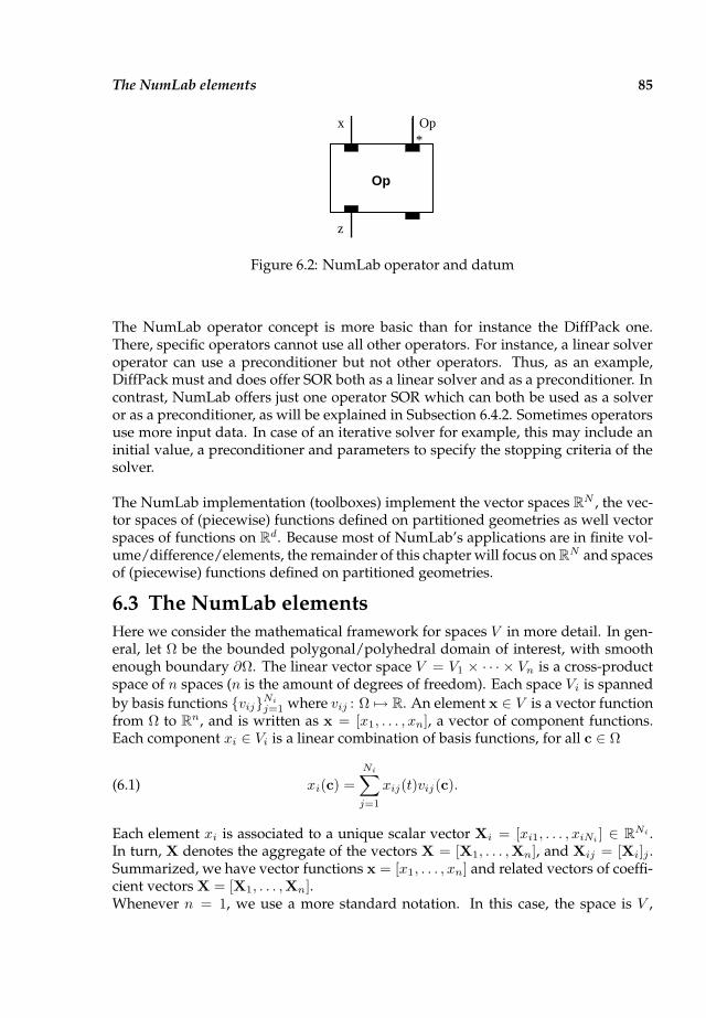
The NumLab elements 85
x
z
*
Op
Op
Figure 6.2: NumLab operator and datum
The NumLab operator concept is more basic than for instance the DiffPack one.There, specific operators cannot use all other operators. For instance, a linear solveroperator can use a preconditioner but not other operators. Thus, as an example,DiffPack must and does offer SOR both as a linear solver and as a preconditioner. Incontrast, NumLab offers just one operator SOR which can both be used as a solveror as a preconditioner, as will be explained in Subsection 6.4.2. Sometimes operatorsuse more input data. In case of an iterative solver for example, this may include aninitial value, a preconditioner and parameters to specify the stopping criteria of thesolver.
The NumLab implementation (toolboxes) implement the vector spaces RN , the vec-tor spaces of (piecewise) functions defined on partitioned geometries as well vectorspaces of functions on Rd. Because most of NumLab’s applications are in finite vol-ume/difference/elements, the remainder of this chapter will focus on R
N and spacesof (piecewise) functions defined on partitioned geometries.
6.3 The NumLab elements
Here we consider the mathematical framework for spaces V in more detail. In gen-eral, let Ω be the bounded polygonal/polyhedral domain of interest, with smoothenough boundary ∂Ω. The linear vector space V = V1 × · · · × Vn is a cross-productspace of n spaces (n is the amount of degrees of freedom). Each space Vi is spanned
by basis functions vijNi
j=1 where vij : Ω 7→ R. An element x ∈ V is a vector functionfrom Ω to R
n, and is written as x = [x1, . . . , xn], a vector of component functions.Each component xi ∈ Vi is a linear combination of basis functions, for all c ∈ Ω
(6.1) xi(c) =
Ni∑
j=1
xij(t)vij(c).
Each element xi is associated to a unique scalar vector Xi = [xi1, . . . , xiNi ] ∈ RNi .
In turn, X denotes the aggregate of the vectors X = [X1, . . . ,Xn], and Xij = [Xi]j .Summarized, we have vector functions x = [x1, . . . , xn] and related vectors of coeffi-cient vectors X = [X1, . . . ,Xn].Whenever n = 1, we use a more standard notation. In this case, the space is V ,
86 Chapter 6: NumLab concepts
spanned by basis functions vjNj=1, and elements x ∈ V are related to coefficientvector x = [x1, . . . , xN ].
For most finite element computations, the basis functions vij of Vi have local support.However, basis functions have global support in spectral finite elements computa-tions. The local supports, also called elements, are created with the use of a triangula-tion algorithm. On the lowest level, NumLab offers vectors in Rn and block matricesin Rn×m for coefficient vectors vijj and Jacobian matrices. Of course, each matrixblock has full, diagonal or sparse representations.
6.4 The NumLab operators
This section discusses the NumLab operators. Here is a small overview on the Num-Lab operators:
1. Problem-specific operators: Transient Finite Element, Volume, Difference opera-tors F for transient boundary value problems (BVPs); Operators which formu-late systems of ordinary differential equations (ODEs); operators which act onlinear operators (for instance image filters);
2. Problem-specific solvers for systems of ODEs: Time-step and time-integration op-erators formulated with the use of (parts of) the problem-specific operatorsmentioned above. The former operators require non-linear solvers for the com-putation of solutions;
3. Solvers for systems of non-linear equations: Such systems are operators, and theirsolution is reduced to the solution of a sequence of linear systems;
4. Solvers for systems of linear equations: Such systems are also operators F(x) =Ax − b. Their solution is reduced to a sequence of operator evaluations andvector space operations.
The reduction from one type of operator to another is commented on in the subsec-tions below, in the reverse order of the itemization above. Thus, Subsection 6.4.1examines systems of (non-)linear equations, Subsection 6.4.2 examines (non-)linearsolvers and preconditioners, Subsection 6.4.4 considers the reduction of systems ofODEs to non-linear systems, and Subsection 6.4.3 deals with an initial boundaryvalue problem. The presented mathematical reductions are de facto standards, newis NumLab’s software implementation which is a one to one mapping of these tech-niques.
6.4.1 Systems of equations
NumLab has no special representation for (non-)linear systems of equations, suchentities are formulated with the use of operators. In NumLab a matrix is a linearoperator F which is of the form x 7→ Ax, where A is the canonical coefficient matrixrepresentation of F (obtained with the canonical basis of vector space V). Next, if

The NumLab operators 87
F is a linear operator and f an element, a linear system of equations is representedwith an affine operator G of the form
(6.2) x 7→ F(x) − f .
In NumLab, an image is a linear operator which simplifies image processing (seeFigure 6.4m).
Non-linear systems of equations are represented by an operator x 7→ F(x) such thata solution of F(x) = 0 solves the non-linear system.
6.4.2 Solvers and Preconditioners
In NumLab, all solvers are represented as operators as well. Each solver S for theproblem z = F−1(x) calculates an approximation of F−1(x) for a specific argumentx and extra argument F. The operator S approximates F−1(x) as follows: it is im-plemented as a fixed point iteration z(k+1) = S(z(k)) with initial value z(0) := z andfinal value z = z(K). By construction, it is not continuous due to a stopping toleranceε > 0 and the maximum amount of iterations, and it is not possible to calculate dSfor a specific x and F.
All of NumLab’s iterative solvers adhere to the following principle: If z(0) ∈ V forsome space V , then
(6.3) z(0) (S)7→ z(1) (S)7→ z(2) (S)7→ z(3) (S)7→ · · · ,
is a sequence in V , i.e., each solver maps V into V . This holds even if V is con-strained, such as V = [1, 2] + λ[3, 4] : λ ∈ R ⊂ R2. This is of importance becauseDirichlet or Neumann boundary conditions as will be discussed in Subsection 6.4.3lead to constrained spaces V . The idea behind (6.3) is that all iterations should mapan approximate solution to a potentially better approximate solution of the problemof interest. This at least requires that all z(k), k > 0 are in the same space as z(0).Furthermore, because this holds, we can switch and mix linear solvers on demand.
As an example, let F be an affine operator (linear system) and consider the Richard-son iterative solver R for the computation of z = F−1(x). This solver is defined withthe use of a fixed point iteration:
(6.4) z(k+1) = z(k) − (F(z(k)) − x),
The evaluation z = R(x) of the Richardson operator R is implemented with the useof NumLab’s basic operations as follows:
(6.5)
r(1)= F(z(k));
r(2)= r− x;
z(k+1) (2)= z(k) − r,

88 Chapter 6: NumLab concepts
with initial value z(0) := z and final value z := z(K). Here(1)= denotes operator eval-
uation and(2)= vector space operation, where the right hand part is assigned to the left
hand side. The computation of the Jacobian is not offered because R is not differen-tiable.
Because iterative solvers can be slow, as detailed in Chapter 3, it is common to usea preconditioner. Richardson method with preconditioner (operator) P passed as anextra operator is:
(6.6) z(k+1) = z(k) −P(F(z(k)) − x).
Now the implementation of the evaluation z = R(x) of the preconditioned Richard-son operator R is:
(6.7)
r(1)= F(z(k));
r(2)= r − x;
s(1)= P(r);
z(k+1) (2)= z(k) − s.
The NumLab toolbox only offers the preconditioned Richardson method with de-fault preconditioner x 7→ x. Each operator (such as x 7→ U−1L−1x) can be used asa preconditioner. Likewise, each solver can use itself as preconditioner, if its maxi-mum amount of iterations is set to for instance 1. It should be noted that differentsolvers use preconditioners in a different manner.
Though preconditioning in NumLab is simple, this does not solve the problem ofproper preconditioning. This has been addressed in Chapter 3 and the applicationdesigner should keep these mathematical restrictions in mind, when designing asuitable solver for the problem at hand.
Similar to linear solvers, NumLab also formulates non-linear solvers as operators.Problems with non-linear operators which do not provide derivative evaluation,can be solved with the use of a fixed point method (comparable to the Richardsonmethod above), or with a combinatorial fixed point method [96] (a multi-dimensionalvariant of the bisection method). Non-linear operators that provide derivative eval-uation can also be solved with (damped, inexact) Newton methods (see [36, 40]).As an example, let x be an element and F an operator, and consider the NumLabundamped Newton’s method U for the calculation of z = F−1(x): The fixed pointiteration is:
(6.8) z(k+1) = z(k) − dF−1(z(k))(F(z(k)) − x),
The NumLab operators 89
and could be implemented as:
(6.9)
r(1)= F(z(k));
r(2)= r − x;
s(1)= inv(dF(z(k)))(r);
z(k+1) (2)= z(k) − r,
where F 7→ inv(dF(z(k))) returns the inverse (linear operator) of the Jacobian of F atz(k). However, NumLab implements Newton’s method differently. It uses a linearsolver R in order to approximate dF(z(k))−1(r):
(6.10)
r(1)= F(z(k));
r(2)= r − x;
s(1)= R(r, Jacobian(F));
z(k+1) (2)= z(k) − r.
The linear solver is passed to Newton’s method as an extra operator, its Jacobianmatrix is calculated and passed to Richardson method. The Richardson solver is alsopassed as an extra operator, which in turns could have been passed a preconditioneras an extra operator.
6.4.3 Partial differential equations
In order to show how NumLab formulates partial differential equations (PDEs) asoperators, consider a PDE. Let d be a positive integer and Ω ⊂ Rd be the boundedregion of interest, and let ∂Ω denote its boundary. The problem of interest is to finda solution u defined on Ω that satisfies
(6.11)−∆u = h in Ω,
u = g at ∂Ω.
For the sake of simplicity of presentation, all boundary conditions are of Dirich-let type. The NumLab construction of the operator depends on the discretizationmethod and on the specific properties desired from the operator: Whenever possible,NumLab operators are maximal monotone (see [64]). This ensures that the Jacobian isa positive (semi-) definite linear operator. For a finite element discretization of (6.11)NumLab defines a maximal monotone operator as follows. First, Ω is covered withelements (see [70]) which serve to define a basis vjNj=1 (see [57]), which generatesthe vector space V of interest. In standard Galerkin finite elements (see [5]), the solu-tion u to (6.11) is assumed to be in the space V , i.e., u =
∑
j ujvj for some coefficient
vector u = [u1, . . . , uN ] ∈ RN . Define E : V 7→ V and f ∈ V as follows:
(6.12) E(u) :=∑
i
[∇
N∑
j=1
ujvj
∇vi − hvi]
vi, f =∑
i
(
hvi
)
vi .
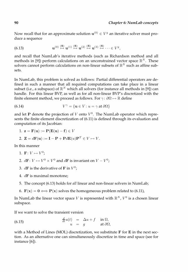
90 Chapter 6: NumLab concepts
Now recall that for an approximate solution u(0) ∈ V g an iterative solver must pro-duce a sequence
(6.13) u(0) (S)7→ u(1) (S)7→ u(2) (S)7→ u(3) (S)7→ · · · ∈ V g,
and recall that NumLab’s iterative methods (such as Richardson method and allmethods in [9]) perform calculations on an unconstrained vector space R
N . Thesesolvers cannot perform calculations on non-linear subsets of RN such as affine sub-sets.
In NumLab, this problem is solved as follows: Partial differential operators are de-fined in such a manner that all required computations can take place in a linearsubset (i.e., a subspace) of RN which all solvers (for instance all methods in [9]) canhandle. For this linear BVP, as well as for all non-linear BVP’s discretized with thefinite element method, we proceed as follows. For γ : ∂Ω 7→ R define
(6.14) V γ = u ∈ V : u = γ at ∂Ω
and let P denote the projection of V onto V 0. The NumLab operator which repre-sents the finite element discretization of (6.11) is defined through its evaluation andcomputation of its Jacobian:
1. z = F(u) := P(E(u) − f) ∈ V
2. Z = dF(u) := I−P + PdE(u)PT ∈ V 7→ V .
In this manner
1. F : V 7→ V 0;
2. dF : V 7→ V 0 × V 0 and dF is invariant on V − V 0;
3. dF is the derivative of F in V 0;
4. dF is maximal monotone;
5. The concept (6.13) holds for all linear and non-linear solvers in NumLab;
6. F(x) = 0 ⇐⇒ P(x) solves the homogeneous problem related to (6.11),
In NumLab the linear vector space V is represented with RN , V 0 is a chosen linearsubspace.
If we want to solve the transient version
(6.15)ddtu(t) = ∆u+ f in Ω,
u = g at ∂Ω,
with a Method of Lines (MOL) discretization, we substitute F for E in the next sec-tion. As an alternative one can simultaneously discretize in time and space (see forinstance [6]).

The NumLab operators 91
6.4.4 Ordinary differential equations
Standard discretizations of ordinary differential equations can also be formulated asoperators whose evaluation reduces to a sequence of vector space operations andfunction evaluations. For instance, let F be a discrete NumLab operator, and con-sider the initial value problem: Find x(t) for which:
(6.16)d
dtx(t) + F(t,x(t)) = 0 (t > 0), x(0) = x0 .
Let h > 0 denote the discrete time-step, and define tk = kh for all k = 0, 1, 2, . . ..Next, let V be the space which is used to approximate x(t) at a specific time t, letvjj be the basis used to this end and let M be the linear operator:
(6.17) [M]i,j = (vj ,vi).
Provided with an approximation x(k) ∈ V of x(tk), a fixed-step Euler backwardmethod determines an approximation x(k+1) ∈ V of x(tk+1)
(6.18) M(x(k+1) − x(k)) = −hE(tk+1,x(k+1)),
which can be rewritten as
(6.19) M(x(k+1) − x(k)) + hE(tk+1,x(k+1)) = 0 .
Define the operator E as follows:
(6.20) E(x) := M(x− x(k)) + hE(tk+1,x).
Then x(k+1) is a solution of E(x) = 0. Of course, E depends on the extra argumentvalues x(k), tk and h. Each time step we have to solve E(x) = 0 for which we canuse a non-linear solver examined above. Note that F is maximal monotone if E isbecause M is a positive semi-definite linear operator. Likewise, in a finite differencesetting, if E is diagonal dominant, so is F. If E is an L-matrix, so if F, etc..
In general, if a NumLab operator depends on another one, its implementation willkeep all properties invariant. Both on a global scale and a lower level (element/stencil-wise) scale.
The approach above generalizes in a straightforward manner to all explicit meth-ods, such as Runge-Kutta type methods [30], as well as to all implicit discretizationmethods, such as Backward Difference Formulas (BDF) [44]. Furthermore, this ap-proach generalizes to the case of fixed and variable timestep integrators (see PEC andPECE [68]). An example is the solution of a Lotka-Volterra predator-prey problem,shown in Fig. 6.4 l.
92 Chapter 6: NumLab concepts
6.5 The NumLab factored out common components
For all offered ODE/PDE discretizations NumLab factors out common components.For the sake of demonstration, we focus on the case of a finite element discretizationsuch as in Section 6.4.3. In NumLab, a finite element function x ∈ V is constructedwith a sequence of entities: In this list, on each line, each first item is input to Num-Lab, and all others are derived (invisible):
1. boundary specification 7→ geometry specification 7→
2. reference element 7→
3. element generator 7→ computational grid (discrete geometry) 7→
4. reference functions 7→
5. boundary conditions 7→ linear and constrained spaces 7→ sampler 7→
6. symbolic function 7→
7. element x in the space V .
For each input alternatives are possible, for instance one can use quadrilateral in-stead of triangular elements. A NumLab network which demonstrates all of theseinput choices can be seen in figure 6.3. The various parts are encircled and num-bered as follows: The grid is defined first (1), followed by the space (2). Then theoperator of interest (3) is constructed, followed by the solver (4). In this example wehave chosen for the CGS iterative method which is preconditioned by an incompletefactorization. Finally, the visualization pipeline is indicated by (5).NumLab’s basic requirements, such as (6.13), are elegantly and efficiently capturedby using an object-oriented approach to software design [18, 28, 77, 83]. Conse-quently, we have implemented our numerical software framework as an object-oriented library written in the C++ language [91]. The sections which follow providemore (implementational) detail about the different factored out components.
6.5.1 The Grid module
Recall the NumLab element definitions in Section 6.3. To be able to define local sup-port for the basis functions vij later on, we need to discretize the function’s domainΩ. This is modeled in the software framework by the Grid module, which coversthe function’s domain with elements e. This Grid module takes a Contour as in-put, which describes the boundary ∂Ω of Ω. The default contour is the unit square’scontour.In NumLab, the grid covers regions Ω in any dimension (e.g. 2D planar, manifoldor 3D spatial), and consists of a variety of element shapes, such as triangles, quadri-laterals, tetrahedra, prisms, hexahedrals, n-simplices (see [70]), and so on. All gridsimplement a common interface. This interface provides several but few services.These include: Iteration over the grid elements and their related vertices, topologicalqueries such as the element which contains a given point. The amount of services
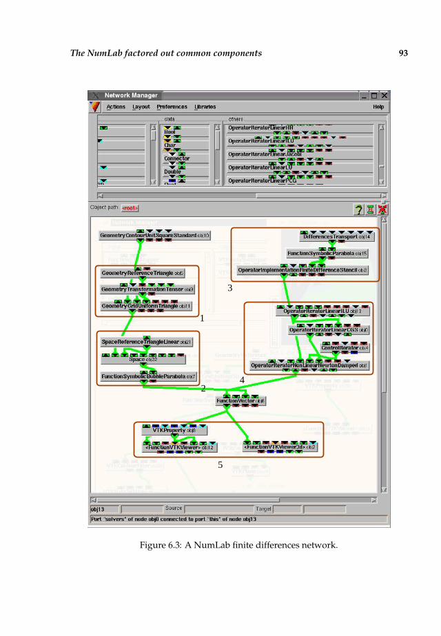
The NumLab factored out common components 93
5
42
1
3
Figure 6.3: A NumLab finite differences network.
94 Chapter 6: NumLab concepts
is a minimum: Modules which use a grid generator and need more service mustcompute the required relations from the provided information.Specific Grid generator modules produce grids in different manners. NumLab con-tains Delaunay generators, simplicial generators, and regular generators, and ”gen-erators”which read an existing grid from a file. An example generator is illustratedin figure 6.4k, which shows a cubic finite element interpolant on a 2-manifold in R3.
6.5.2 The Space module
The linear vector space V is implemented by the software module Space. Spacetakes a Grid and BoundaryConditions as inputs. The grid’s discretization incombination with the boundary conditions are used to build the supports of its basisfunctions vij . The default boundary conditions are Dirichlet type conditions for allsolution components. None, Robin, Neumann and vectorial boundary conditionsare specified per boundary part. Recall that elements in V do not have to satisfy theDirichlet boundary conditions.Because Grid has a minimal interface, some information, required by Space for theconstruction of the basis functions, is not provided. Whenever this happens, Spaceinternally computes the required information with the use of Grid’s services.
A specific Space module implements a specific set of basis functions, such as con-stant, linear, quadratic, or even higher order polynomial degree, matched to the el-ements’ geometry. The interface of the Space module follows the mathematicalproperties of the vector space V presented so far: Elements x,y ∈ V can be addedtogether or scaled by real values. Furthermore, elements vij of V are functions, andV permits evaluation at points c ∈ Ω of such functions and their derivatives.It should be kept in mind that elements of V are functions, not linear combinationsof functions. Therefore, the name Space is somewhat misleading. However, for thebrevity of demonstration, the name Space will also be used in the sequel.
In most cases the required basis functions have local support, also called element-wisesupport. The restriction of global basis function vij to support e is said to be localfunction vir. In software, this is coded as follows: For space component i (so Vi),element e, and local basis function r thereon, j := j(i, r) induces basis functionvij . The software implementation is on element-level for efficiency purposes: Givena point c ∈ Ω, Space determines which support e contains c for the evaluation ofvij(c).
6.5.3 The Function module
As discussed, a vector function x : Ω 7→ Rn in a space V generated by vij is uniquelyrelated to a coefficient vector X with coefficients Xij . Based on this observation,NumLab software module Function implements a vector function x as a block vec-tor of real-valued coefficients Xij , combined with a reference to the related Space,which contains related functions vij .The Functionmodule provides services to evaluate the function and its derivativesat a given point c ∈ Ω. To this end, both x’s coefficient vector X and the point c are

The NumLab factored out common components 95
passed to the Space module referred to by x. In turn, the Space module returnsthe value of x(c). This is computed following the definition x(c) = [
∑
j xijvij(c)],as described in the previous section. The computation of the partial derivatives of agiven function x in a point c follows a similar implementation.
Providing evaluation of functions x ∈ V and of their derivatives at given points is,strictly speaking, the minimal interface the Space module has to implement. How-ever, it is sometimes convenient to be able to evaluate a function at a point givenas an element number and local coordinates within that element. This is especiallyimportant for efficiency in the case where one operation is iterated over all elementsof a Grid, such as in the case of numerical integration. If the Space module allowsevaluating functions at points specified as elements and local element coordinates,the implementation of the numerical integration is considerably faster than whenpoint-to-element location has to be performed. Consequently, we also provided theSpace module with a function evaluation interface which accepts an element num-ber and a point defined in the element local coordinates.
6.5.4 The Operator module
As described previously, an operator F : V 7→ W maps an element x ∈ V to an el-ement z ∈ W . The evaluation z = G(x) computes the coefficients zij of z from thecoefficients xij of x, as well as from the bases vij and wij of V and W respec-tively. Next to the evaluation of G, derivatives such as the Jacobian operator DG
of G are evaluated in a similar manner. Such derivatives are important in severalapplications. For example, they can be used in order to find a solution of G(z) = x,by Newton’s method.
The software implementation of the operator notion follows straightforwardly themathematical concepts introduced in Section 6.4. The implementation is done bythe Operator module, which offers two services: evaluation of z = G(x), codedas G.eval(z,x), and of the Jacobian of G in point y, z = DG(y)x, coded asG.getJ(y).eval(z,x). To evaluate z = G(x), the Operator module takes twoFunction objects z and x as input and computes the coefficients zij using the coeffi-cients xij and the bases of the Space objects z and x carry with them. It is importantthat both the ’input’ z and the ’output’ x of the Operator module are provided,since it is in this way that Operators determine the spaces V , respectively W .
To evaluate z = DG(y)x, the Operator proceeds similarly. Internally, DG(y) isusually implemented as a coefficient matrix, and the operation DG(y)x is a matrix-vector multiplication. However, the implementation details are hidden from the user(DG(y)x may be computed element-wise, i.e. matrix-free), who works only with theFunction and Operator mathematical notions.
Specific Operator implementations differ in the way they compute the above twoevaluations. For example, a simple Diffusion operator z = G(x) may operate ona scalar function and produce a function z where zi = xi−1 − 2xi + xi+1. A genericLinear operator may produce a vector of coefficients z = Ax where A is a matrix.A Summator operator z = G1(x) + G2(x) may take two inputs G1 and G2 andproduce a vector of coefficients zi = [G1(x)]i + [G2(x)]i. Remark that the modules

96 Chapter 6: NumLab concepts
implementing the Linear and Summator operators actually have two inputs each.In both cases the function x is the first input, while the second is the matrix A for theLinear operator and the operators G1 and G2 for the Summator operator. Thesevalues could be as well hard-coded in the operator implementation. In both caseshowever, we see Operator as a function of a single variable x, as described in themathematical framework.
6.5.5 The Solver module
We model the solving of G(z) = x by the module Solver in our software frame-work. Mathematically, Solver is similar to an operator S : V 7→ W , where V andW are function spaces. The interface of Solver provides evaluation at functionsx ∈ W, similarly to the Operator module. The implementation of the Solverevaluation operation z = S(x) should provide an approximation z to z ≈ F−1(x).However, Solver does not provide evaluation of its Jacobian, as this may be unde-sirably complex to compute in the general case.
Practically, Solver takes as input an initial guess Function object x and an Operatorobject G. Its output z is such that G(z) = x. The operations done by the solverare either vector space operations or Operator evaluations, or evaluations of sim-ilar operators G(z). In the actual implementation, this is modeled by providing theSolver module with one or more extra inputs of type Solver. In this way, one canfor example connect a nested chain of preconditioners to an iterative solver module.
The implementation of a specific Solver follows straightforwardly from its mathe-matical description. Iterative solvers such as Richardson, SOR, CG, Bi-CG, with orwithout preconditioners, are easily implemented in this software framework.
The framework makes no distinction between a solver and a preconditioner, as dis-cussed in Section 6.4. The sole difference between a solver and a preconditioner inthis framework is semantic, not structural. A solver is supposed to produce an exactsolution of G(z) = 0 (up to a desired numerical accuracy), whereas the precondi-tioner is supposed to return an approximate one. Both are implemented as Solvermodules, which allows easy cascading of a chain of preconditioners to an iterativesolver as well as using preconditioners and solvers interchangeably in applications.Furthermore, the framework makes no structural distinction between direct and it-erative solvers. For example, an ILUSolver module is implemented to computean incomplete LU factorization (cf. Subsection 3.4.3) of its input operator G. TheILUSolver module can be used as a preconditioner for a ConjugateGradientsolver module. In the case the ILUSolver is not connected to the Conjugate-Gradient module’s input, the latter performs non preconditioned computations.Alternatively, a LUSolver module is implemented to provide a complete LU factor-ization of its input operator G (see Chapter 2). The LUSolver can be used eitherdirectly to solve the equation G(z) = x, or as preconditioner for another Solvermodule.
6.5.6 NumLab components
The natural modeling of the mathematics in terms of class hierarchies, the object-oriented design allows users to easily extend the current framework with new soft-
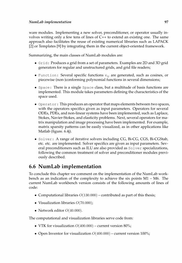
NumLab implementation 97
ware modules. Implementing a new solver, preconditioner, or operator usually in-volves writing only a few tens of lines of C++ to extend an existing one. The sameapproach also facilitates the reuse of existing numerical libraries such as LAPACK[2] or Templates [9] by integrating them in the current object-oriented framework.
Summarizing, the main classes of NumLab modules are:
• Grid: Produces a grid from a set of parameters. Examples are 2D and 3D gridgenerators for regular and unstructured grids, and grid file readers;
• Function: Several specific functions vij are generated, such as cosines, orpiecewise (non-)conforming polynomial functions in several dimensions;
• Space: There is a single Space class, but a multitude of basis functions areimplemented. This module takes parameters defining the characteristics of thespace used.
• Operator: This produces an operator that maps elements between two spaces,with the operators specifics given as input parameters. Operators for severalODEs, PDEs, and non-linear systems have been implemented, such as Laplace,Stokes, Navier-Stokes, and elasticity problems. Next, several operators for ma-trix manipulation and image processing have been implemented. For example,matrix sparsity patterns can be easily visualized, as in other applications likeMatlab (figure. 6.4j).
• Solver: A range of iterative solvers including CG, Bi-CG, CGS, Bi-CGStab,etc. etc. are implemented. Solver specifics are given as input parameters. Sev-eral preconditioners such as ILU are also provided as Solver specializations,following the common treatment of solver and preconditioner modules previ-ously described.
6.6 NumLab implementation
To conclude this chapter we comment on the implementation of the NumLab work-bench as an indication of the complexity to achieve the six points M1 – M6. Thecurrent NumLab workbench version consists of the following amounts of lines ofcode:
• Computational libraries O(130.000) – contributed as part of this thesis;
• Visualization libraries O(70.000);
• Network editor O(40.000).
The computational and visualization libraries serve code from:
• VTK for visualization O(400.000) – current version 80%;
• Open Inventor for visualization O(400.000) – current version 100%;

98 Chapter 6: NumLab concepts
• LAPACK BLAS for computations O(1.000.000) - current version 10%;
• SEPRAN for computations O(1.000.000) - current version 1%.
A NumLab application which makes use of computations and visualization is linkedto an average of 40 to 50 different libraries.
To finish with, the NumLab workbench runs on Linux and Silicon Graphics sys-tems with the appropriate versions of all libraries. In order to facilitate its mainte-nance, processes are automated as much as is possible. The emphasis is on the au-tomated construction of wrappers for external libraries such as VTK, Open Inventorand SEPRAN.
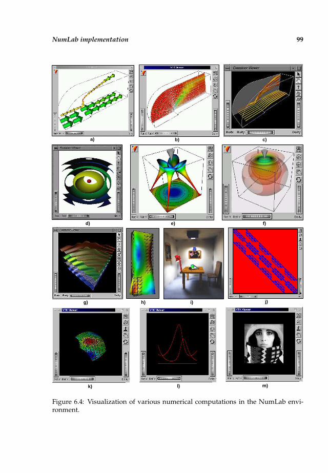
NumLab implementation 99
d) e) f)
g) h) i) j)
k) l) m)
a) b) c)
Figure 6.4: Visualization of various numerical computations in the NumLab envi-ronment.

Chapter 7
NumLab preconditioners
In this chapter we examine the implementation of the approximate inverse precon-ditioner of Chapter 4 as part of the NumLab workbench. The NumLab concept hasbeen described in Chapter 6. In this chapter we show how the approximate inversepreconditioner is implemented as part of NumLab and how this new tool is used forresearch purposes. The implementation of our new tool, the approximate inversepreconditioner, is described in Section 7.1. As detailed in Chapter 1 we are interestedin grids with a brick-like structure, and in particular in grids with several levels ofrefinement. For such grids and the model problem in (7.1) of interest we illustratethe effectiveness of the approximate inverse preconditioner by means of several ex-amples. In Section 7.2 some one dimensional examples are considered first, followedin Section 7.3 and Section 7.4 by more realistic two and three dimensional examples.
7.1 Introduction
In this section we describe how preconditioning techniques can be embedded insidethe NumLab workbench, and in particular the approximate inverse preconditioner.Recall from Chapter 3 the convection diffusion equation
(7.1)−a∆u+ b · ∇u+ cu = f in Ω = (0, 1)d ⊂ Rd,
u = g at ∂Ω,
and the resulting linear system of equations
(7.2) Anxn = bn
obtained after discretization of (7.1).The approximate inverse preconditioner Gn from Chapter 4 is implemented in anew module. Given the input of a linear operator An, this module first constructsthe approximate inverse Gn and subsequently evaluates a vector xn whenever calledupon. We apply this preconditioner to speed up the CGS iterative method as detailedin Section 3.1. As the implementation into NumLab can be copied line by line, weonly give the lines relevant for the preconditioning steps. For a full implementa-tion of the CGS algorithm see [103]. The matrix-vector multiplications are denotedin operator notation as detailed in Section 6.2. So, the matrix-vector multiplication
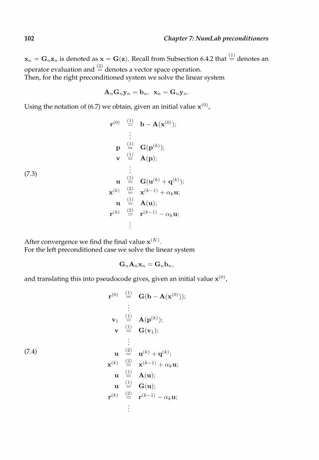
102 Chapter 7: NumLab preconditioners
xn = Gnzn is denoted as x = G(z). Recall from Subsection 6.4.2 that(1)= denotes an
operator evaluation and(2)= denotes a vector space operation.
Then, for the right preconditioned system we solve the linear system
AnGnyn = bn, xn = Gnyn.
Using the notation of (6.7) we obtain, given an initial value x(0),
(7.3)
r(0) (1)= b −A(x(0));...
p(1)= G(p(k));
v(1)= A(p);...
u(1)= G(u(k) + q(k));
x(k) (2)= x(k−1) + αku;
u(1)= A(u);
r(k) (2)= r(k−1) − αku;...
After convergence we find the final value x(K).For the left preconditioned case we solve the linear system
GnAnxn = Gnbn,
and translating this into pseudocode gives, given an initial value x(0),
(7.4)
r(0) (1)= G(b −A(x(0)));...
v1(1)= A(p(k));
v(1)= G(v1);...
u(2)= u(k) + q(k);
x(k) (2)= x(k−1) + αku;
u(1)= A(u);
u(1)= G(u);
r(k) (2)= r(k−1) − αku;...
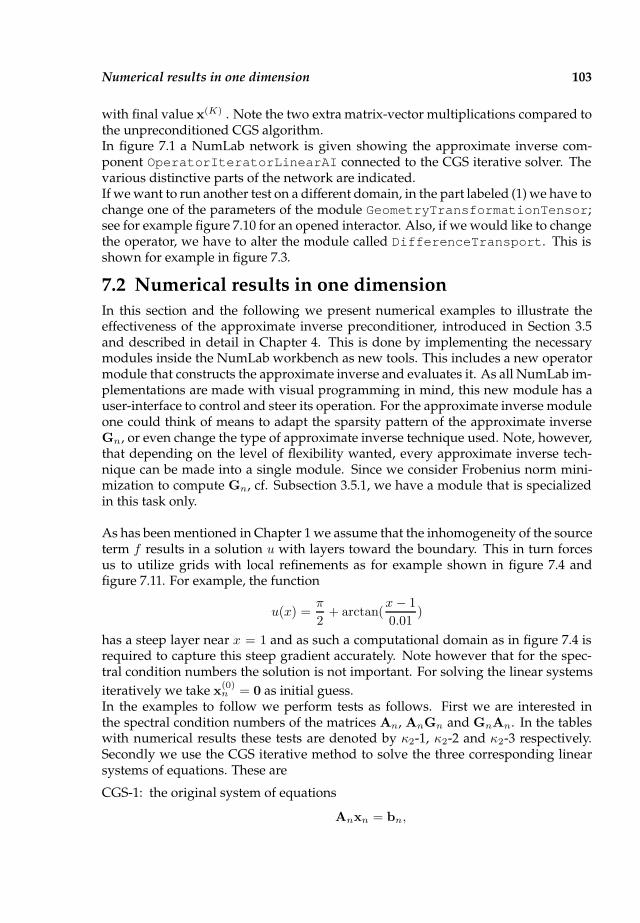
Numerical results in one dimension 103
with final value x(K) . Note the two extra matrix-vector multiplications compared tothe unpreconditioned CGS algorithm.In figure 7.1 a NumLab network is given showing the approximate inverse com-ponent OperatorIteratorLinearAI connected to the CGS iterative solver. Thevarious distinctive parts of the network are indicated.If we want to run another test on a different domain, in the part labeled (1) we have tochange one of the parameters of the module GeometryTransformationTensor;see for example figure 7.10 for an opened interactor. Also, if we would like to changethe operator, we have to alter the module called DifferenceTransport. This isshown for example in figure 7.3.
7.2 Numerical results in one dimension
In this section and the following we present numerical examples to illustrate theeffectiveness of the approximate inverse preconditioner, introduced in Section 3.5and described in detail in Chapter 4. This is done by implementing the necessarymodules inside the NumLab workbench as new tools. This includes a new operatormodule that constructs the approximate inverse and evaluates it. As all NumLab im-plementations are made with visual programming in mind, this new module has auser-interface to control and steer its operation. For the approximate inverse moduleone could think of means to adapt the sparsity pattern of the approximate inverseGn, or even change the type of approximate inverse technique used. Note, however,that depending on the level of flexibility wanted, every approximate inverse tech-nique can be made into a single module. Since we consider Frobenius norm mini-mization to compute Gn, cf. Subsection 3.5.1, we have a module that is specializedin this task only.
As has been mentioned in Chapter 1 we assume that the inhomogeneity of the sourceterm f results in a solution u with layers toward the boundary. This in turn forcesus to utilize grids with local refinements as for example shown in figure 7.4 andfigure 7.11. For example, the function
u(x) =π
2+ arctan(
x− 1
0.01)
has a steep layer near x = 1 and as such a computational domain as in figure 7.4 isrequired to capture this steep gradient accurately. Note however that for the spec-tral condition numbers the solution is not important. For solving the linear systems
iteratively we take x(0)n = 0 as initial guess.
In the examples to follow we perform tests as follows. First we are interested inthe spectral condition numbers of the matrices An, AnGn and GnAn. In the tableswith numerical results these tests are denoted by κ2-1, κ2-2 and κ2-3 respectively.Secondly we use the CGS iterative method to solve the three corresponding linearsystems of equations. These are
CGS-1: the original system of equations
Anxn = bn,
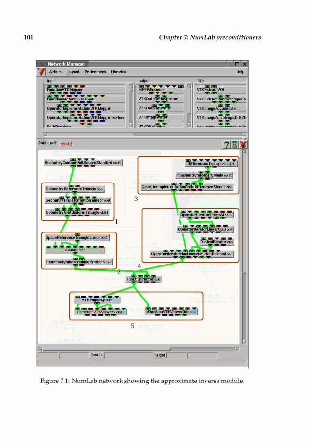
104 Chapter 7: NumLab preconditioners
3
5
1
24
Figure 7.1: NumLab network showing the approximate inverse module.
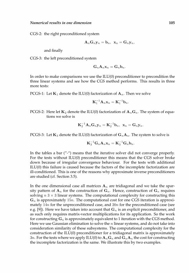
Numerical results in one dimension 105
CGS-2: the right preconditioned system
AnGnyn = bn, xn = Gnyn,
and finally
CGS-3: the left preconditioned system
GnAnxn = Gnbn.
In order to make comparisons we use the ILU(0) preconditioner to precondition thethree linear systems and see how the CGS method performs. This results in threemore tests:
PCGS-1: Let K1 denote the ILU(0) factorization of An. Then we solve
K−11 Anxn = K−1
1 bn.
PCGS-2: Here let K2 denote the ILU(0) factorization of AnGn. The system of equa-tions we solve is
K−12 AnGnyn = K−1
2 bn, xn = Gnyn.
PCGS-3: Let K3 denote the ILU(0) factorization of GnAn. The system to solve is
K−13 GnAnxn = K−1
3 Gnbn.
In the tables a bar (”-“) means that the iterative solver did not converge properly.For the tests without ILU(0) preconditioner this means that the CGS solver brokedown because of irregular convergence behaviour. For the tests with additionalILU(0) this failure is caused because the factors of the incomplete factorization areill-conditioned. This is one of the reasons why approximate inverse preconditionersare studied (cf. Section 3.5).
In the one dimensional case all matrices An are tridiagonal and we take the spar-sity pattern of An for the construction of Gn. Hence, construction of Gn requiressolving n 3 × 3 linear systems. The computational complexity for constructing thisGn is approximately 15n. The computational cost for one CGS iteration is approxi-mately 14n for the unpreconditioned case, and 20n for the preconditioned case (seee.g. [9]). Here we have taken into account that Gn is an explicit preconditioner, andas such only requires matrix-vector multiplications for its application. So the workfor constructing Gn is approximately equivalent to 1 iteration with the CGS method.Here we use Gaussian elimination to solve the n linear systems, and do not take intoconsideration similarity of these subsystems. The computational complexity for theconstruction of the ILU(0) preconditioner for a tridiagonal matrix is approximately3n. For the tests where we apply ILU(0) to AnGn and GnAn the cost for constructingthe incomplete factorization is the same. We illustrate this by two examples.

106 Chapter 7: NumLab preconditioners
0 1
Figure 7.2: A grid with refinement to x = 1, ψ = 1/2.
Example 7.1. In this example we consider the grid depicted in figure 7.2 with refine-ment factor ψ = 1/2. Let n > 0 and let f := 1/ψn+1. Then the grid points xi aregiven by (cf. (4.2))
(7.5) xi =f (1−i/(n+1)) − f
1 − f, ∀i = 0, . . . , n+ 1.
After using the boundary conditions in x0 and xn+1 we obtain an n×n linear systemof equations. First we consider the pure diffusive case, a = 1 and b = c = 0. Theresults are given in table 7.1.
1-D, number of unknownsn 4 5 6 7 8 9 10 11
κ2-1 119.92 497.60 2027.81 8188.27 3.29·104 1.32·105 5.28·105 2.12·106
κ2-2 13.75 39.41 60.15 168.92 249.04 696.75 1014.12 2833.04κ2-3 2.87 5.33 4.86 7.56 6.97 9.76 9.12 11.94
CGS-1 5 7 10 13 18 - - -CGS-2 2 5 3 7 4 9 10 11CGS-3 2 5 3 7 4 9 5 11PCGS-1 - - - - - - - -PCGS-2 1 - - - - - - -PCGS-3 1 1 1 1 1 1 3 1
Table 7.1: Results for grid 7.1, ψ = 1/2, diffusion only.
We see from this table that κ2(An) is O(h−2), and that the CGS method breaks downfor n ≥ 9. For the two preconditioned linear systems, κ2(GnAn) behaves as pre-dicted by the estimate in Property 4.26, despite the fact we consider here GnAn
instead of the modified matrix Bln in (4.13). For the other product AnGn we observe
κ2(AnGn) ≈ O(h−1) as in (4.29). For the tests with the ILU(0) preconditioner wesee that this preconditioner breaks down because of ill-conditioned factors when ap-plied to An and AnGn. Judging from the number of iterations needed to convergethe combination of the ILU(0) preconditioner and the matrix GnAn seems to be areal winner. It should be noted that additional to the construction of Gn the con-struction of the incomplete factors of GnAn is required, which means an increase incomputational complexity. However, this does not amount to the complexity of 1extra iteration.
Next we consider the same grid but now with a convective term b∇u added. Forour NumLab network this means we have to alter an input parameter in the modulethat defines the differential operator. This is illustrated in figure 7.3 in which we have
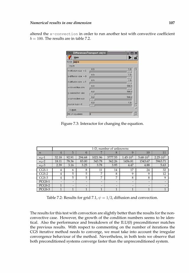
Numerical results in one dimension 107
altered the x-convection in order to run another test with convective coefficientb = 100. The results are in table 7.2.
Figure 7.3: Interactor for changing the equation.
1-D, number of unknownsn 4 5 6 7 8 9 10 11
κ2-1 32.18 92.91 294.68 1021.96 3777.55 1.45·104 5.68·105 2.25·105
κ2-2 18.11 78.36 83.00 343.78 362.26 1456.81 1543.67 5963.71κ2-3 2.39 3.16 3.25 3.78 3.95 4.47 4.88 5.63
CGS-1 4 6 8 11 14 17 24 32CGS-2 4 5 5 7 8 9 9 12CGS-3 4 5 5 7 7 8 8 9PCGS-1 - - - - - - - -PCGS-2 1 - - - - - - -PCGS-3 1 1 1 1 1 1 1 1
Table 7.2: Results for grid 7.1, ψ = 1/2, diffusion and convection.
The results for this test with convection are slightly better than the results for the non-convective case. However, the growth of the condition numbers seems to be iden-tical. Also the performance and breakdown of the ILU(0) preconditioner matchesthe previous results. With respect to commenting on the number of iterations theCGS iterative method needs to converge, we must take into account the irregularconvergence behaviour of the method. Nevertheless, in both tests we observe thatboth preconditioned systems converge faster than the unpreconditioned system.

108 Chapter 7: NumLab preconditioners
0 1
Figure 7.4: A grid with refinement to x = 0 and x = 1, ψ = 1/2.
Example 7.2. To conclude with the one dimensional examples we look at the grid infigure 7.4 which resembles a simple representation of a brick. Let m > 0 such thatn = 2m+ 1 and let f := 1/ψm+1. Then the grid points xi for this grid are given by
(7.6) xi =
1/2− f(2i/(n+1))−f2(1−f) , 0 ≤ i < m+ 1,
1/2, i = m+ 1,
1/2 + f(2−2i/(n+1))−f2(1−f) , m+ 1 < i ≤ n+ 1.
We consider the purely diffusive case. The results are displayed in table 7.3.
1-D, number of unknownsn 3 5 7 9 11 13 15 17 19
κ2-1 4.57 21.53 99.14 425.24 1761.62 7171.82 2.89·104 1.16·105 4.66·105
κ2-2 1.50 6.33 16.75 37.58 76.40 164.02 321.86 679.88 1319.49κ2-3 1.68 3.12 4.29 5.37 6.72 7.54 9.03 9.72 11.28
CGS-1 2 3 5 7 14 14 - 22 -CGS-2 2 3 4 5 12 7 12 11 17CGS-3 2 3 4 5 8 7 10 9 11PCGS-1 1 1 - - - - - - -PCGS-2 1 1 1 - - - - - -PCGS-3 1 1 1 1 1 1 1 1 1
Table 7.3: Results for grid 7.4, ψ = 1/2, diffusion only.
We observe a growth of κ2(An) proportional to h−2, of κ2(AnGn) proportional toh−1 and of κ2(GnAn) proportional to log(h−1). Also in this example we observebreakdown of the CGS method for the unpreconditioned system, and faster conver-gence for the two preconditioned systems. Furthermore, preconditioning An andAnGn with ILU(0) fails because of ill-conditioned factors. This nullifies the fact thatpreconditioning An with ILU(0) works for two problem sizes. Again, ILU(0) appliedto GnAn (PCGS-3) is the best.
In figure 7.5 the norms of the residuals at each iteration step are given for n = 13and n = 15. The irregular convergence of the CGS method for solving the unprecon-ditioned system (CGS-1) is clearly visible in the left hand figure; the stagnation ofthe iterative process becomes clear in the right hand figure. Furthermore we see thatthe iterative process for solving the two preconditioned systems converges muchsmoother.
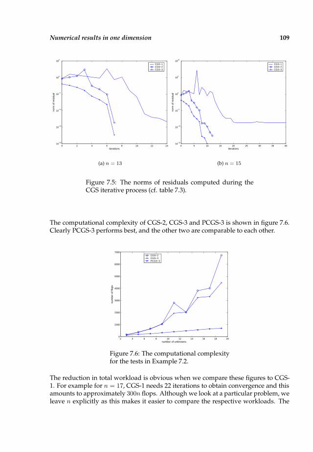
Numerical results in one dimension 109
0 2 4 6 8 10 12 1410
−20
10−15
10−10
10−5
100
105
iterations
norm
of r
esid
ual
CGS−1CGS−2CGS−3
(a) n = 13
0 5 10 15 20 25 30 35 4010
−15
10−10
10−5
100
105
1010
iterations
norm
of r
esid
ual
CGS−1CGS−2CGS−3
(b) n = 15
Figure 7.5: The norms of residuals computed during theCGS iterative process (cf. table 7.3).
The computational complexity of CGS-2, CGS-3 and PCGS-3 is shown in figure 7.6.Clearly PCGS-3 performs best, and the other two are comparable to each other.
2 4 6 8 10 12 14 16 18 200
1000
2000
3000
4000
5000
6000
7000
number of unknowns
num
ber
of fl
ops
CGS−2CGS−3PCGS−3
Figure 7.6: The computational complexityfor the tests in Example 7.2.
The reduction in total workload is obvious when we compare these figures to CGS-1. For example for n = 17, CGS-1 needs 22 iterations to obtain convergence and thisamounts to approximately 300n flops. Although we look at a particular problem, weleave n explicitly as this makes it easier to compare the respective workloads. The
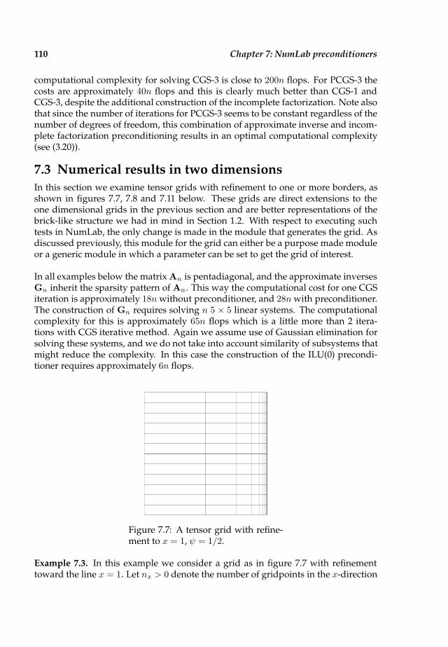
110 Chapter 7: NumLab preconditioners
computational complexity for solving CGS-3 is close to 200n flops. For PCGS-3 thecosts are approximately 40n flops and this is clearly much better than CGS-1 andCGS-3, despite the additional construction of the incomplete factorization. Note alsothat since the number of iterations for PCGS-3 seems to be constant regardless of thenumber of degrees of freedom, this combination of approximate inverse and incom-plete factorization preconditioning results in an optimal computational complexity(see (3.20)).
7.3 Numerical results in two dimensions
In this section we examine tensor grids with refinement to one or more borders, asshown in figures 7.7, 7.8 and 7.11 below. These grids are direct extensions to theone dimensional grids in the previous section and are better representations of thebrick-like structure we had in mind in Section 1.2. With respect to executing suchtests in NumLab, the only change is made in the module that generates the grid. Asdiscussed previously, this module for the grid can either be a purpose made moduleor a generic module in which a parameter can be set to get the grid of interest.
In all examples below the matrix An is pentadiagonal, and the approximate inversesGn inherit the sparsity pattern of An. This way the computational cost for one CGSiteration is approximately 18n without preconditioner, and 28n with preconditioner.The construction of Gn requires solving n 5 × 5 linear systems. The computationalcomplexity for this is approximately 65n flops which is a little more than 2 itera-tions with CGS iterative method. Again we assume use of Gaussian elimination forsolving these systems, and we do not take into account similarity of subsystems thatmight reduce the complexity. In this case the construction of the ILU(0) precondi-tioner requires approximately 6n flops.
Figure 7.7: A tensor grid with refine-ment to x = 1, ψ = 1/2.
Example 7.3. In this example we consider a grid as in figure 7.7 with refinementtoward the line x = 1. Let nx > 0 denote the number of gridpoints in the x-direction

Numerical results in two dimensions 111
and let f := 1/ψn+1. Then the x-coordinates in figure 7.7 are given by
(7.7) xi =f (1−i/(nx+1)) − f
1− f, ∀i = 0, . . . , nx + 1.
Let ny denote the number of gridpoints in the y-directions. The y-coordinates arethen given by yi = i/(ny + 1), i = 0, . . . , ny + 1. Then n = nxny is the total numberof degrees of freedom. In this example and the following nx = ny . We examine thecondition numbers and number of CGS iterations for a pure diffusive problem.
2-D, number of unknowns (number of refinement steps)n (l) 16 (4) 25 (5) 36 (6) 49 (7) 64 (8) 81 (9) 100 (10) 121 (11)
κ2-1 62.53 244.71 973.81 3895.24 1.56·104 6.24·104 2.50·105 9.99·105
κ2-2 5.03 11.08 24.68 53.54 111.48 231.74 476.91 974.03κ2-3 2.63 3.73 4.72 6.19 7.39 8.98 10.27 11.99CGS-1 10 50 - - - - - -CGS-2 8 10 12 15 16 20 21 22CGS-3 8 10 11 14 14 18 17 19PCGS-1 7 - - - - - - -PCGS-2 5 5 7 - - - - -PCGS-3 5 5 5 6 6 6 7 7
Table 7.4: Results for grid 7.7, ψ = 1/2, diffusion only.
From table 7.4 we observe the following for the spectral condition numbers. κ2(An)grows proportional to h−2 and κ2(AnGn) grows proportional to h−1 which means areduction by an order of h−1. GnAn seems to be conditioned best with κ2(GnAn)
.=
O(log(h−1)). With respect to convergence of the CGS method we see that the methodbreaks down for solving with An for l ≥ 6 with l being the number of refinementsteps. Solving the systems with AnGn and GnAn results in an equivalent numberof iterations. This changes when an ILU(0) preconditioner is considered. An withILU(0) breaks down quickly because the factors are unstable. This is also the case forAnGn with additional ILU(0) preconditioner. In contrast, the ILU(0) factorization ofGnAn does not show these instabilities and helps to reduce the number of iterationsfurther. Also the growth of the number of iterations for this test seems less than forthe test without additional ILU(0) preconditioner.

112 Chapter 7: NumLab preconditioners
Figure 7.8: A tensor grid with refine-ment to x = 1 and y = 1, ψ = 1/2.
Example 7.4. Next we examine grids as in figure 7.8 with refinement to the linesx = 1 and y = 1. The x-coordinates are as in (7.7) and the y-coordinates are computedin the same way. We consider the purely diffusive case first. The results are given intable 7.5.
2-D, number of unknowns (number of refinement steps)n (l) 16 (4) 25 (5) 36 (6) 49 (7) 64 (8) 81 (9) 100 (10) 121 (11)
κ2-1 121.61 506.14 2066.41 8352.85 3.36·104 1.35·105 5.40·105 2.16·106
κ2-2 8.03 20.89 40.12 92.64 172.70 391.37 718.89 1612.62κ2-3 2.78 3.83 4.80 5.90 6.92 8.03 9.08 10.19
CGS-1 11 21 37 - - - - -CGS-2 9 13 14 16 17 19 20 23CGS-3 8 11 11 13 15 16 17 18PCGS-1 - - - - - - - -PCGS-2 5 7 - - - - - -PCGS-3 4 5 5 5 5 6 6 6
Table 7.5: Results for grid 7.8, ψ = 1/2, diffusion only.
Next we are interested to see the influence of a convective term b · ∇u. Thereforeconsider convection in both directions with b = [100, 100]T . In figure 7.9 the cor-responding NumLab interactor is shown, with the parameters x-convection andy-convection set to 100. The results are given in table 7.6.
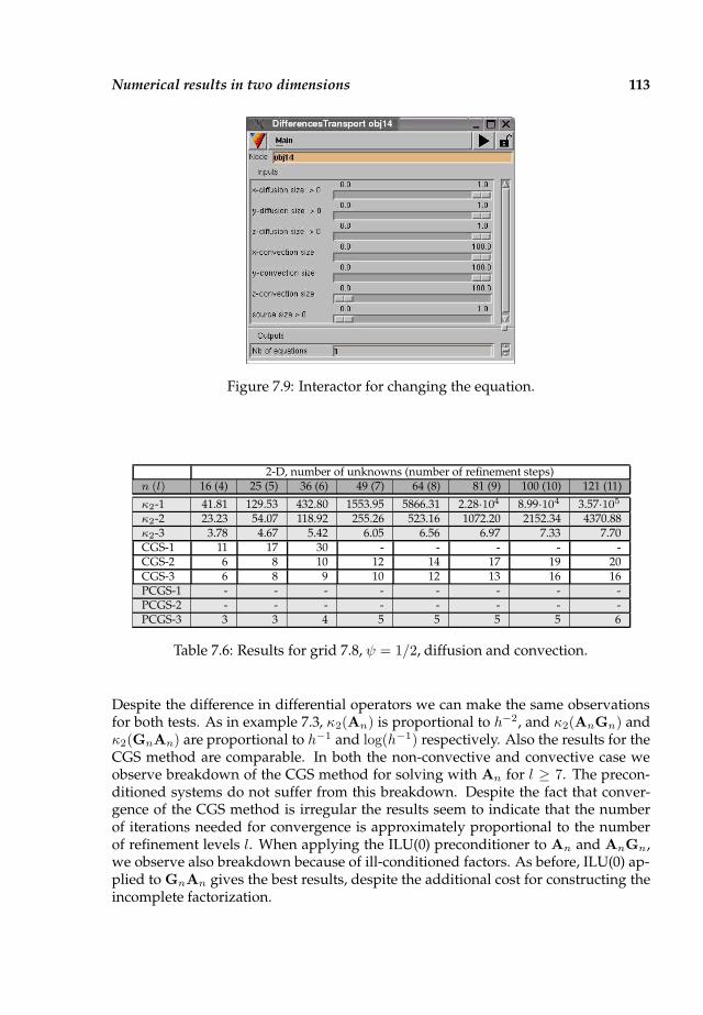
Numerical results in two dimensions 113
Figure 7.9: Interactor for changing the equation.
2-D, number of unknowns (number of refinement steps)n (l) 16 (4) 25 (5) 36 (6) 49 (7) 64 (8) 81 (9) 100 (10) 121 (11)
κ2-1 41.81 129.53 432.80 1553.95 5866.31 2.28·104 8.99·104 3.57·105
κ2-2 23.23 54.07 118.92 255.26 523.16 1072.20 2152.34 4370.88κ2-3 3.78 4.67 5.42 6.05 6.56 6.97 7.33 7.70CGS-1 11 17 30 - - - - -CGS-2 6 8 10 12 14 17 19 20CGS-3 6 8 9 10 12 13 16 16PCGS-1 - - - - - - - -PCGS-2 - - - - - - - -PCGS-3 3 3 4 5 5 5 5 6
Table 7.6: Results for grid 7.8, ψ = 1/2, diffusion and convection.
Despite the difference in differential operators we can make the same observationsfor both tests. As in example 7.3, κ2(An) is proportional to h−2, and κ2(AnGn) andκ2(GnAn) are proportional to h−1 and log(h−1) respectively. Also the results for theCGS method are comparable. In both the non-convective and convective case weobserve breakdown of the CGS method for solving with An for l ≥ 7. The precon-ditioned systems do not suffer from this breakdown. Despite the fact that conver-gence of the CGS method is irregular the results seem to indicate that the numberof iterations needed for convergence is approximately proportional to the numberof refinement levels l. When applying the ILU(0) preconditioner to An and AnGn,we observe also breakdown because of ill-conditioned factors. As before, ILU(0) ap-plied to GnAn gives the best results, despite the additional cost for constructing theincomplete factorization.
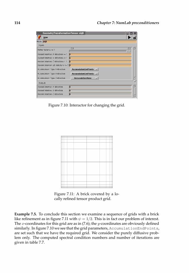
114 Chapter 7: NumLab preconditioners
Figure 7.10: Interactor for changing the grid.
Figure 7.11: A brick covered by a lo-cally refined tensor product grid.
Example 7.5. To conclude this section we examine a sequence of grids with a bricklike refinement as in figure 7.11 with ψ = 1/2. This is in fact our problem of interest.The x-coordinates for this grid are as in (7.6); the y-coordinates are obviously definedsimilarly. In figure 7.10 we see that the grid parameters, AccumulationEndPoints,are set such that we have the required grid. We consider the purely diffusive prob-lem only. The computed spectral condition numbers and number of iterations aregiven in table 7.7.
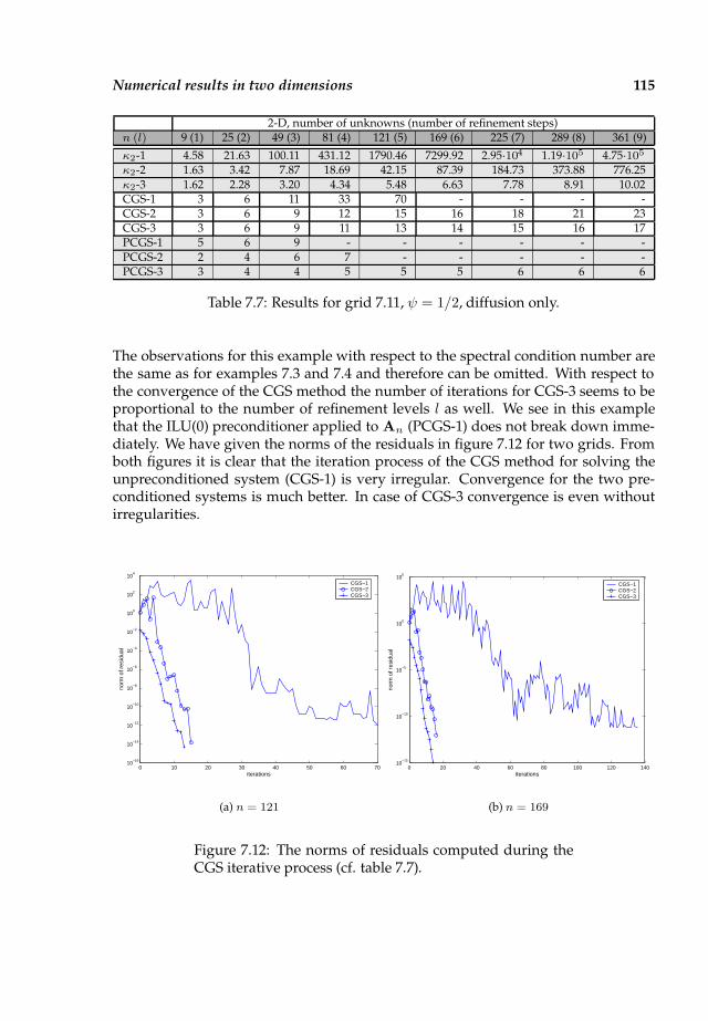
Numerical results in two dimensions 115
2-D, number of unknowns (number of refinement steps)n (l) 9 (1) 25 (2) 49 (3) 81 (4) 121 (5) 169 (6) 225 (7) 289 (8) 361 (9)
κ2-1 4.58 21.63 100.11 431.12 1790.46 7299.92 2.95·104 1.19·105 4.75·105
κ2-2 1.63 3.42 7.87 18.69 42.15 87.39 184.73 373.88 776.25κ2-3 1.62 2.28 3.20 4.34 5.48 6.63 7.78 8.91 10.02CGS-1 3 6 11 33 70 - - - -CGS-2 3 6 9 12 15 16 18 21 23CGS-3 3 6 9 11 13 14 15 16 17PCGS-1 5 6 9 - - - - - -PCGS-2 2 4 6 7 - - - - -PCGS-3 3 4 4 5 5 5 6 6 6
Table 7.7: Results for grid 7.11, ψ = 1/2, diffusion only.
The observations for this example with respect to the spectral condition number arethe same as for examples 7.3 and 7.4 and therefore can be omitted. With respect tothe convergence of the CGS method the number of iterations for CGS-3 seems to beproportional to the number of refinement levels l as well. We see in this examplethat the ILU(0) preconditioner applied to An (PCGS-1) does not break down imme-diately. We have given the norms of the residuals in figure 7.12 for two grids. Fromboth figures it is clear that the iteration process of the CGS method for solving theunpreconditioned system (CGS-1) is very irregular. Convergence for the two pre-conditioned systems is much better. In case of CGS-3 convergence is even withoutirregularities.
0 10 20 30 40 50 60 7010
−16
10−14
10−12
10−10
10−8
10−6
10−4
10−2
100
102
104
iterations
norm
of r
esid
ual
CGS−1CGS−2CGS−3
(a) n = 121
0 20 40 60 80 100 120 14010
−15
10−10
10−5
100
105
iterations
norm
of r
esid
ual
CGS−1CGS−2CGS−3
(b) n = 169
Figure 7.12: The norms of residuals computed during theCGS iterative process (cf. table 7.7).
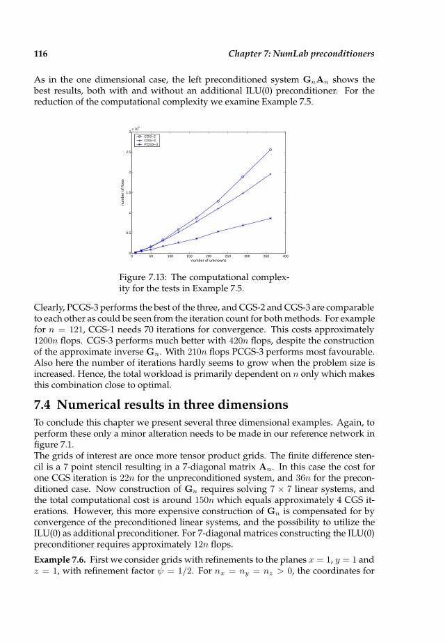
116 Chapter 7: NumLab preconditioners
As in the one dimensional case, the left preconditioned system GnAn shows thebest results, both with and without an additional ILU(0) preconditioner. For thereduction of the computational complexity we examine Example 7.5.
0 50 100 150 200 250 300 350 4000
0.5
1
1.5
2
2.5
3x 10
5
number of unknowns
num
ber
of fl
ops
CGS−2CGS−3PCGS−3
Figure 7.13: The computational complex-ity for the tests in Example 7.5.
Clearly, PCGS-3 performs the best of the three, and CGS-2 and CGS-3 are comparableto each other as could be seen from the iteration count for both methods. For examplefor n = 121, CGS-1 needs 70 iterations for convergence. This costs approximately1200n flops. CGS-3 performs much better with 420n flops, despite the constructionof the approximate inverse Gn. With 210n flops PCGS-3 performs most favourable.Also here the number of iterations hardly seems to grow when the problem size isincreased. Hence, the total workload is primarily dependent on n only which makesthis combination close to optimal.
7.4 Numerical results in three dimensions
To conclude this chapter we present several three dimensional examples. Again, toperform these only a minor alteration needs to be made in our reference network infigure 7.1.The grids of interest are once more tensor product grids. The finite difference sten-cil is a 7 point stencil resulting in a 7-diagonal matrix An. In this case the cost forone CGS iteration is 22n for the unpreconditioned system, and 36n for the precon-ditioned case. Now construction of Gn requires solving 7 × 7 linear systems, andthe total computational cost is around 150n which equals approximately 4 CGS it-erations. However, this more expensive construction of Gn is compensated for byconvergence of the preconditioned linear systems, and the possibility to utilize theILU(0) as additional preconditioner. For 7-diagonal matrices constructing the ILU(0)preconditioner requires approximately 12n flops.
Example 7.6. First we consider grids with refinements to the planes x = 1, y = 1 andz = 1, with refinement factor ψ = 1/2. For nx = ny = nz > 0, the coordinates for
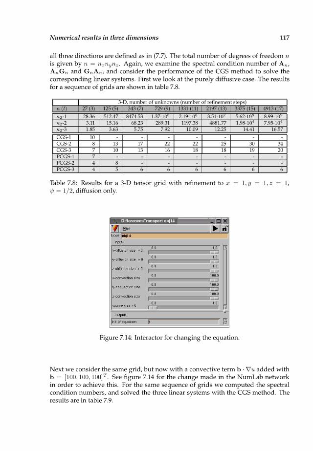
Numerical results in three dimensions 117
all three directions are defined as in (7.7). The total number of degrees of freedom nis given by n = nxnynz . Again, we examine the spectral condition number of An,AnGn and GnAn, and consider the performance of the CGS method to solve thecorresponding linear systems. First we look at the purely diffusive case. The resultsfor a sequence of grids are shown in table 7.8.
3-D, number of unknowns (number of refinement steps)n (l) 27 (3) 125 (5) 343 (7) 729 (9) 1331 (11) 2197 (13) 3375 (15) 4913 (17)
κ2-1 28.36 512.47 8474.53 1.37·105 2.19·106 3.51·107 5.62·198 8.99·109
κ2-2 3.11 15.16 68.23 289.31 1197.38 4881.77 1.98·104 7.95·104
κ2-3 1.85 3.63 5.75 7.92 10.09 12.25 14.41 16.57
CGS-1 10 - - - - - - -CGS-2 8 13 17 22 22 25 30 34CGS-3 7 10 13 16 18 18 19 20PCGS-1 7 - - - - - - -PCGS-2 4 8 - - - - - -PCGS-3 4 5 6 6 6 6 6 6
Table 7.8: Results for a 3-D tensor grid with refinement to x = 1, y = 1, z = 1,ψ = 1/2, diffusion only.
Figure 7.14: Interactor for changing the equation.
Next we consider the same grid, but now with a convective term b · ∇u added withb = [100, 100, 100]T . See figure 7.14 for the change made in the NumLab networkin order to achieve this. For the same sequence of grids we computed the spectralcondition numbers, and solved the three linear systems with the CGS method. Theresults are in table 7.9.
118 Chapter 7: NumLab preconditioners
3-D, number of unknowns (number of refinement steps)n (l) 27 (3) 125 (5) 343 (7) 729 (9) 1331 (11) 2197 (13) 3375 (15) 4913 (17)
κ2-1 16.07 166.60 2143.91 3.23·104 5.11·105 8.16·106 1.31·108 2.09·109
κ2-2 8.16 51.83 271.05 1143.05 4627.43 1.87·104 7.53·104 3.02·105
κ2-3 3.26 6.35 8.77 10.18 10.93 11.59 12.49 13.57
CGS-1 10 36 - - - - - -CGS-2 5 9 13 20 23 26 31 35CGS-3 5 8 13 16 18 21 22 23PCGS-1 4 - - - - - - -PCGS-2 3 6 - - - - - -PCGS-3 3 4 5 6 6 7 7 7
Table 7.9: Results for a 3-D tensor grid with refinement to x = 1, y = 1, z = 1,ψ = 1/2, diffusion and convection.
One can make similar remarks about these two examples as were made for the exam-ples in one and two dimensions. κ2(An) is once more proportional to h−2, κ2(AnGn)to h−1 and κ2(GnAn) to log(h−1). Furthermore, the CGS method breaks down forAn, and ILU(0) is unstable for both An and AnGn.
Example 7.7. As a final example we consider tensor grids with refinement to all sixborders of the cube. This resembles the discretization of a brick 3-D. In figure 7.18a network is shown with the modules that create this three dimensional tensor grid.The module GeometryContourCube defines the domain Ω, in this case (0, 1)3. Thetensor grid itself is shown as well. The coordinates in all three directions are asin (7.6), for nx = ny = nz > 0. First we look at the diffusive case. The results aregiven in table 7.10.
3-D, number of unknowns (number of refinement steps)n (l) 27 (1) 125 (2) 343 (3) 729 (4) 1331 (5) 2197 (6) 3375 (7) 4913 (8)
κ2-1 4.58 21.73 100.99 436.25 1815.35 7410.06 2.99·104 1.20·105
κ2-2 1.60 2.89 5.97 14.20 32.64 68.88 143.50 295.01κ2-3 1.55 2.22 3.01 4.16 5.36 6.56 7.73 8.85
CGS-1 4 10 29 - - - - -CGS-2 4 8 11 13 16 16 17 19CGS-3 4 8 10 11 14 13 17 16PCGS-1 5 7 9 - - - - -PCGS-2 3 4 5 7 9 - - -PCGS-3 3 4 4 5 5 6 6 6
Table 7.10: Results for a 3-D tensor grid with brick refinement, ψ = 1/2,diffusion only.
Next we examine the same sequence of grids, but now with a convective term added.Hence let b = [100, 100, 100]T (see figure 7.14). The results for these tests are intable 7.11.
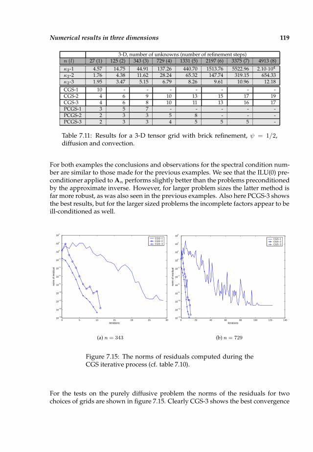
Numerical results in three dimensions 119
3-D, number of unknowns (number of refinement steps)n (l) 27 (1) 125 (2) 343 (3) 729 (4) 1331 (5) 2197 (6) 3375 (7) 4913 (8)
κ2-1 4.57 14.75 44.91 137.26 440.70 1513.76 5522.96 2.10·104
κ2-2 1.76 4.38 11.62 28.24 65.32 147.74 319.15 654.33κ2-3 1.95 3.47 5.15 6.79 8.26 9.61 10.96 12.18
CGS-1 10 - - - - - - -CGS-2 4 6 9 10 13 15 17 19CGS-3 4 6 8 10 11 13 16 17PCGS-1 3 5 7 - - - - -PCGS-2 2 3 3 5 8 - - -PCGS-3 2 3 3 4 5 5 5 -
Table 7.11: Results for a 3-D tensor grid with brick refinement, ψ = 1/2,diffusion and convection.
For both examples the conclusions and observations for the spectral condition num-ber are similar to those made for the previous examples. We see that the ILU(0) pre-conditioner applied to An performs slightly better than the problems preconditionedby the approximate inverse. However, for larger problem sizes the latter method isfar more robust, as was also seen in the previous examples. Also here PCGS-3 showsthe best results, but for the larger sized problems the incomplete factors appear to beill-conditioned as well.
0 5 10 15 20 25 3010
−16
10−14
10−12
10−10
10−8
10−6
10−4
10−2
100
102
104
iterations
norm
of r
esid
ual
CGS−1CGS−2CGS−3
(a) n = 343
0 20 40 60 80 100 120 14010
−14
10−12
10−10
10−8
10−6
10−4
10−2
100
102
104
106
iterations
norm
of r
esid
ual
CGS−1CGS−2CGS−3
(b) n = 729
Figure 7.15: The norms of residuals computed during theCGS iterative process (cf. table 7.10).
For the tests on the purely diffusive problem the norms of the residuals for twochoices of grids are shown in figure 7.15. Clearly CGS-3 shows the best convergence
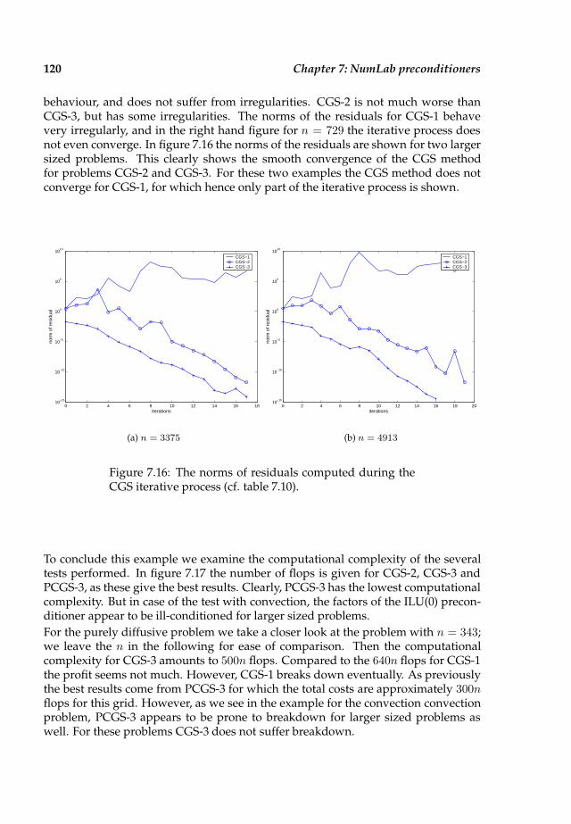
120 Chapter 7: NumLab preconditioners
behaviour, and does not suffer from irregularities. CGS-2 is not much worse thanCGS-3, but has some irregularities. The norms of the residuals for CGS-1 behavevery irregularly, and in the right hand figure for n = 729 the iterative process doesnot even converge. In figure 7.16 the norms of the residuals are shown for two largersized problems. This clearly shows the smooth convergence of the CGS methodfor problems CGS-2 and CGS-3. For these two examples the CGS method does notconverge for CGS-1, for which hence only part of the iterative process is shown.
0 2 4 6 8 10 12 14 16 1810
−15
10−10
10−5
100
105
1010
iterations
norm
of r
esid
ual
CGS−1CGS−2CGS−3
(a) n = 3375
0 2 4 6 8 10 12 14 16 18 2010
−15
10−10
10−5
100
105
1010
iterations
norm
of r
esid
ual
CGS−1CGS−2CGS−3
(b) n = 4913
Figure 7.16: The norms of residuals computed during theCGS iterative process (cf. table 7.10).
To conclude this example we examine the computational complexity of the severaltests performed. In figure 7.17 the number of flops is given for CGS-2, CGS-3 andPCGS-3, as these give the best results. Clearly, PCGS-3 has the lowest computationalcomplexity. But in case of the test with convection, the factors of the ILU(0) precon-ditioner appear to be ill-conditioned for larger sized problems.
For the purely diffusive problem we take a closer look at the problem with n = 343;we leave the n in the following for ease of comparison. Then the computationalcomplexity for CGS-3 amounts to 500n flops. Compared to the 640n flops for CGS-1the profit seems not much. However, CGS-1 breaks down eventually. As previouslythe best results come from PCGS-3 for which the total costs are approximately 300nflops for this grid. However, as we see in the example for the convection convectionproblem, PCGS-3 appears to be prone to breakdown for larger sized problems aswell. For these problems CGS-3 does not suffer breakdown.
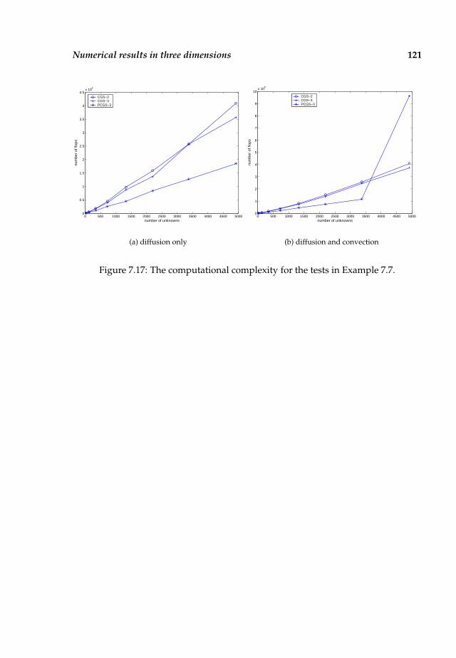
Numerical results in three dimensions 121
0 500 1000 1500 2000 2500 3000 3500 4000 4500 50000
0.5
1
1.5
2
2.5
3
3.5
4
4.5x 10
6
number of unknowns
num
ber
of fl
ops
CGS−2CGS−3PCGS−3
(a) diffusion only
0 500 1000 1500 2000 2500 3000 3500 4000 4500 50000
1
2
3
4
5
6
7
8
9
10x 10
6
number of unknowns
num
ber
of fl
ops
CGS−2CGS−3PCGS−3
(b) diffusion and convection
Figure 7.17: The computational complexity for the tests in Example 7.7.

122 Chapter 7: NumLab preconditioners
Figure 7.18: A NumLab network for a three dimensional grid withbrick-like refinement, see Example 7.7.
Chapter 8
Conclusions and future work
Preconditioning techniques are important for efficiently solving linear systems ofequations. This holds in particular for problems for which standard methods do notwork satisfactorily. Among such problems are those for which the non-smooth so-lution requires employing a computational grid with local refinements. Apart fromthe need for efficient preconditioners and solution methods, the possibility of testingnewly developed tools without too much effort is equally important. This has leadto the NumLab computational platform. Both topics have been discussed in this the-sis. In this final chapter we give the major conclusions firsts, followed by severalrecommendations for future research.
8.1 Conclusions
The major conclusions are the following.
• A Gaussian elimination strategy based on a special node numbering schemewas considered for grids with refinements along a line. This strategy resultedin an O(n logn) computational complexity and compares well with the fill-in-optimized minimum degree algorithm.
• The standard estimate for the spectral condition number is not sharp for gridswith local refinements.
• Related to the brick wall problem we have a convection diffusion equationwhich after discretization leads to a matrix An. For this matrix an approxi-mate inverse preconditioner Gn based on Frobenius norm minimization wasconsidered. In a one dimensional setting theoretical estimates for the spectralcondition number of a modified version Bn of the left preconditioned matrixGnAn; we obtained κ2(Bn)
.= O(n).
Numerical tests showed that this estimate is sharp in one, two and three di-mensions. We observed:
κ2(An).= O(h−2),
κ2(AnGn).= O(h−1),
κ2(GnAn).= O(log(h−1)).
124 Chapter 8: Conclusions and future work
• In one and in two dimensions right multiplication of An by the approximateinverse matrix Gn results in a reducible matrix AnGn. This matrix can be per-muted and written as a 2 × 2 block matrix. This gives rise to various recursivealgorithms that employ this decoupling. Moreover, when An is a discretizationof the Laplace operator, so are the two submatrices of AnGn.
• Solving iteratively the unpreconditioned and preconditioned linear systemsshowed that the original unpreconditioned problem is prone to break downdue to irregular convergence behaviour. Both preconditioned problems seemto perform similarly. Additionally, an incomplete factorization of the matrixAn results in ill-conditioned factors. Hence, solving the original problem pre-conditioned by ILU(0) is subject to breakdown as well. This is also seen whenthe right preconditioned system with AnGn is (additionally) preconditionedby an incomplete factorization. In contrast, solving the left preconditionedsystem shows much improvement when preconditioned by ILU(0). This com-bination of an approximate inverse preconditioner and an incomplete factor-ization appears to be the best strategy with respect to computational complex-ity. However, for large problem sizes this incomplete factorization gives ill-conditioned factors as well. Because of this phenomenon the right precondi-tioned system by the approximate inverse preconditioner is considered to bemost robust overall.
• The NumLab workbench offers a powerful tool to run numerical simulations.Given the generic interface and the implementation of mathematical conceptsas operators, there is a maximum amount of flexibility and freedom in chang-ing the various modules that together constitute a simulation.
8.2 Directions for the future
For both major topics some recommendations for future work can be given.As for the mathematical component there are several aspects that need further re-search. In Chapter 2 only complete Gaussian elimination was considered, whichgave rise to a direct solver. Of interest is to examine the effectiveness of incompletefactorizations (ILU) (Subsection 3.4.3) employed as preconditioner for the number-ing scheme presented in that chapter. Given the fact that the fill-in is almost opti-mal for a complete factorization, incomplete factorization methods of the ILU(p) andILUT variant are thought to be beneficial.Secondly, for the approximate inverse preconditioner discussed in Chapter 4 weonly gave theoretical results for the one dimensional case. Of interest is to exam-ine in detail such preconditioners in higher dimensions and establish estimates forthe (spectral) condition numbers of the matrices AnGn and GnAn. Furthermore,the decoupling phenomenon in Chapter 5 should be exploited further, especially intwo dimensions. Another point for future work is examination of the approximateinverse preconditioner constructed as an approximate left inverse, i.e., GnAn ≈ In.
With respect to the NumLab workbench there are several steps in front of us to-
Directions for the future 125
ward an even more complete workbench. A first start is to merge available (parallel)Finite Element assemblers (such as SEPRAN), integrating problem-specialized itera-tive solvers and preconditioners.Of particular research interest are the optimal multigrid/multilevel type solvers (seeSection 3.4). These can be used within the NumLab framework, but right now nospecial support is provided. In order to offer convenient multigrid/multilevel solvermodules, a few modules need to be extended and others must be added. The gridand solution data types must be extended to handle internal stacks of grids and so-lutions. Restriction and prolongation require new modules, and application-specificpreconditioners are desirable. The strong coupling between the grid and basic itera-tive solvers need not be a problem: operator evaluation can be grid based.From a practical point of view, solving large PDE problems in NumLab is still slowerthan specialized toolkits. This is due to the generic nature of the NumLab modulesthat cannot make assumptions about specific data storage or discretization proper-ties provided by other modules. This problem can be tackled in several ways: im-plementing less generic (optimized) modules, re-engineering the generic modules’implementations to make more extensive use of data caching, or parallelizing thenumerical code. A second limitation involves the need to program new Operatorsubclasses, e.g., to model new PDEs (see Section 6.5.4). A better approach would beto design generic Operators that accept their definition via a symbolic, interpretednotation. Implementing such generic Operators would raise the same efficiencyproblems outlined above.Finally, from a technical point of view, separating the address space of the graphicaleditor from the address space where all modules execute should be another futuregoal. In this way NumLab applications will be more stable and less prone to breakdown when contributed research-modules fail. Also, the computational modulesand visualization viewer module should be run on different threads so data can bevisualized while computations continue.


Appendix A
Pentadiagonal Toeplitz matrices
In this appendix we give an result from [52] related to pentadiagonal Toeplitz matri-ces.
First note that the product of two Toeplitz matrices is close to, but not a Toeplitzmatrix. Let A and B be two 5 × 5 matrices given by
A =
x 1 0 0 01 x 1 0 00 1 x 1 00 0 1 x 10 0 0 1 x
, and B =
y 1 0 0 01 y 1 0 00 1 y 1 00 0 1 y 10 0 0 1 y
.
Then for the product we have
AB =
1 + x y x+ y 1 0 0x+ y 2 + x y x+ y 1 0
1 x+ y 2 + x y x+ y 10 1 x+ y 2 + x y x+ y0 0 1 x+ y 1 + x y
which is not a Toeplitz matrix.
Then we have a result from [52]. Let a, b, x ∈ C. Assume that
An(a, b) =
a b 1 0 0b a b 1 01 b a b 1
0 1 b a b. . .
0 0 1 b a. . .
. . .. . .
. . .
∈ Rn×n,
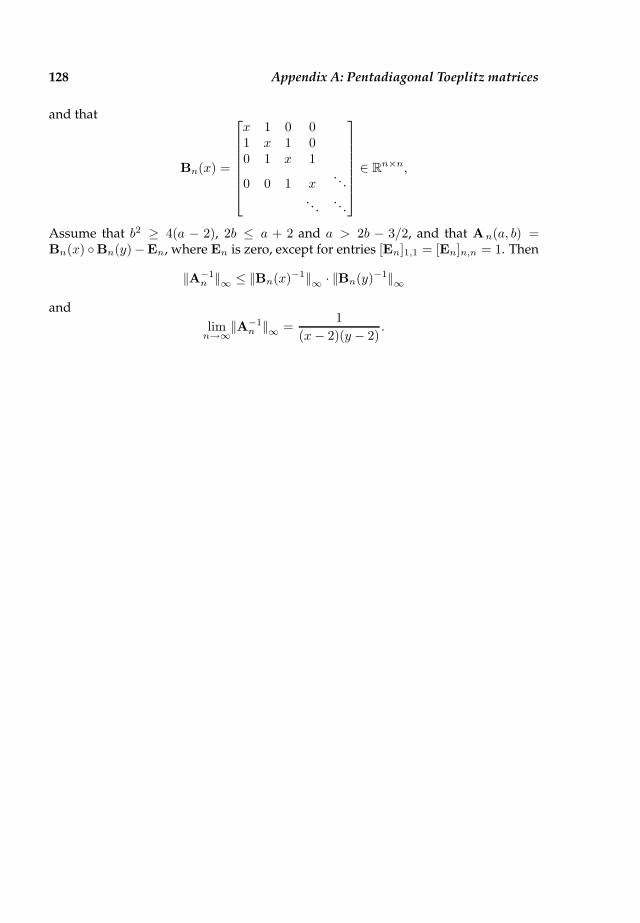
128 Appendix A: Pentadiagonal Toeplitz matrices
and that
Bn(x) =
x 1 0 01 x 1 00 1 x 1
0 0 1 x. . .
. . .. . .
∈ Rn×n,
Assume that b2 ≥ 4(a − 2), 2b ≤ a + 2 and a > 2b − 3/2, and that An(a, b) =Bn(x) Bn(y)−En, where En is zero, except for entries [En]1,1 = [En]n,n = 1. Then
||A−1n ||∞ ≤ ||Bn(x)
−1||∞ · ||Bn(y)−1||∞
and
limn→∞
||A−1n ||∞ =
1
(x− 2)(y − 2).

Appendix B
Turing completeness
This appendix demonstrates that with the addition of certain basic modules, theNumLab visual programming language of Chapter 6 is Turing complete. In Sec-tion B.1 the concepts of alphabet and language are introduced first, followed in Sec-tion B.2 by Turing machines. Then Section B.3 presents the NumLab module designfor primitive recursive functions. The last Section B.4 presents the NumLab moduledesign for µ-recursive functions. Able to imitate µ-recursive functions, NumLab isTuring complete.
B.1 Alphabets and language
The definitions of string, alphabet and language are taken from [65, pp. 29–31]:
Definition B.1.
• An alphabet is finite set of symbols, such as the Roman alphabet a, b, c, ..., z or the binary alphabet 0, 1.
• A string over an alphabet Σ is a finite sequence of symbols from alphabet Σ.
• The set of all strings - including the empty string - over an alphabet Σ is denoted byΣ∗.
These definitions permit the definition of a language:
Definition B.2. A language is set of strings over an alphabet Σ.
Note that in particular a language over σ is a subset of Σ∗. Turing machines aredefined using languages.
B.2 The Turing machine
We start by introducing the concept of a Turing machine. We describe a Turing ma-chine keeping figure B.1 in mind.A Turing machine consists of a tape and a finite-state machine, called control unit. Thecontrol unit disposes over a head to read from and/or write to the tape. In each step,the control unit reads the tape and then performs the following tasks:

130 Appendix B: Turing completeness
3 . 1 4
Finite control
Read/write head(moves in both directions)
h s
s
s
0
1
3 s2
# #
Figure B.1: A Turing machine
• Put the control unit in a new state;
• Either:
– Write a symbol on the current square on the tape or
– Move the read/write head one position to the left (’L’) or to the right (’R’).
The tape has a left end, but is unbounded on the right side. However, in a finitenumbers of steps, the machine can only visit a finite number of squares on the tape.(In case the machine tries to move its head to the left off the end of the tape, it ceasesto operate).
Initially, the tape contains only symbols at the left end. The rest of the tape consistsof blank symbols. The machine is free to alter its input or write on the blank end ofthe tape. The message (data) left at the end of the computation is called the answer.The end of computations is reached when the control unit reaches the halt state. Theblank symbol will be denoted by #.
s1 s1s2s2
s3s3
s0s0
3 1 4
Read/write head(moves in both directions)
h h
f(x)= sin(x)x f(x)
.# #. ## 0
Figure B.2: A Turing machine which imitates a the sine-function
As an example, consider figure B.2. The Turing machine shown computes f(x) =sin(x). Here x = 3.14 is the input the tape. So, to start with, the tape contains the

The Turing machine 131
symbols 3, ., 1 and 4, and the control unit is in state s1. At the end of the computa-tions, the control unit is in the halt state h and has left behind the answer 0 on thetape.
The following definition of a Turing machine comes from [65]:
Definition B.3. A Turing machine is a quadruple (K,Σ, δ, s) where
• K is a finite set of states, not containing the halt state denoted by h;
• Σ is an alphabet, containing the blank symbol #, but not containing the the symbolsL and R;
• s ∈ K is the initial state;
• δ is a function from K × Σ to (K ∪ h) × (Σ ∪ L,R).
With the use of this definition, we can define when a (mathematical) function isTuring computable – required to prove the Turing completeness of NumLab:
Definition B.4. Turing computable functions:Let Σ0 and Σ1 be alphabets not containing the blank symbol #. Let f be a a function from Σ∗
0
to Σ∗1. A Turing machine M = (K,Σ, δ, s) is said to compute f if Σ0, Σ1 ⊆ Σ and for any
w ∈ Σ∗0, if f(w) = u then
(B.1) (s,#w# `∗M (h,#u#).
If such a Turing machine M exists, then f is said to be a Turing computable function.
Because a Turing machine can carry out any computation that can be carried out byany similar type of automata, and because these automata seem to capture the essen-tial features of real computing machines, we take the Turing machine to be a preciseformal equivalent of the intuitive notion of ”algorithm”. Following Church’s Thesisor Church-Turing’s Thesis, nothing will be considered an algorithm if it cannot be ren-dered as a Turing machine. It is a thesis, not a theorem, because it is not a mathemat-ical result: It simply asserts that a certain informal concept corresponds to a certainmathematical object. It is theoretically possible, however, that Church’s Thesis couldbe overthrown at some future date, if someone were to propose an alternative modelof computation that was publicly acceptable as fulfilling the requirement of ”finitelabour at each step”and yet was provably capable of carrying out computations thatcannot be carried out by any Turing machine. No one considers this likely.
A language is called Turing complete, if it can generate all Turing computable func-tions (see also [65]). In this small section, it is shown that NumLab is Turing com-plete, if a few fundamental modules are added.
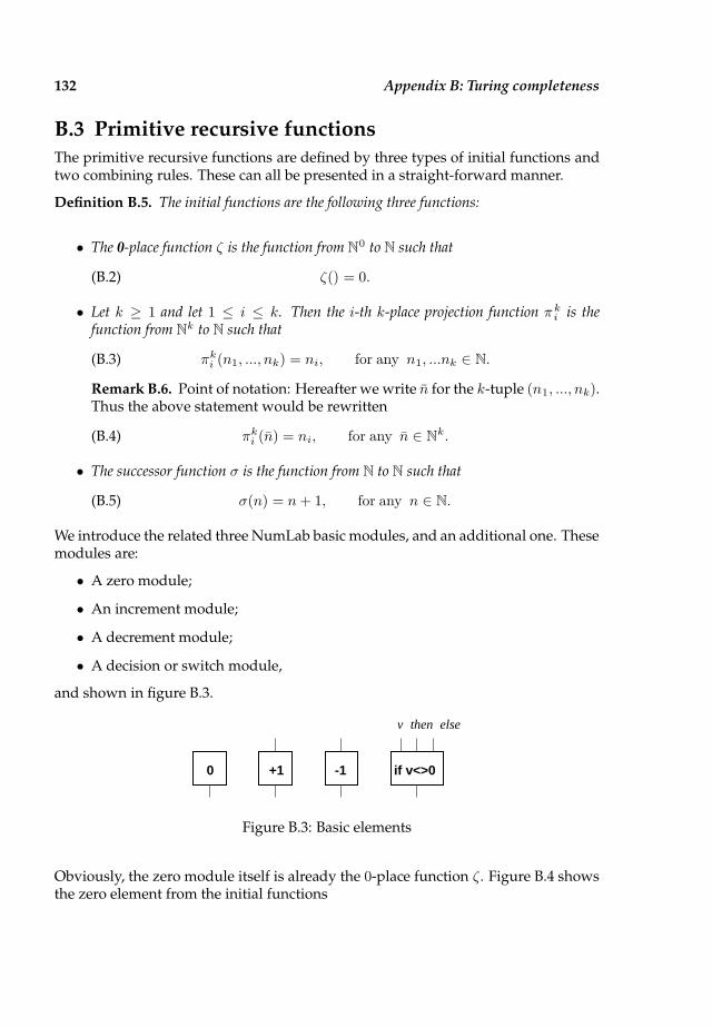
132 Appendix B: Turing completeness
B.3 Primitive recursive functions
The primitive recursive functions are defined by three types of initial functions andtwo combining rules. These can all be presented in a straight-forward manner.
Definition B.5. The initial functions are the following three functions:
• The 0-place function ζ is the function from N0 to N such that
(B.2) ζ() = 0.
• Let k ≥ 1 and let 1 ≤ i ≤ k. Then the i-th k-place projection function πki is thefunction from Nk to N such that
(B.3) πki (n1, ..., nk) = ni, for any n1, ...nk ∈ N.
Remark B.6. Point of notation: Hereafter we write n for the k-tuple (n1, ..., nk).Thus the above statement would be rewritten
(B.4) πki (n) = ni, for any n ∈ Nk.
• The successor function σ is the function from N to N such that
(B.5) σ(n) = n+ 1, for any n ∈ N.
We introduce the related three NumLab basic modules, and an additional one. Thesemodules are:
• A zero module;
• An increment module;
• A decrement module;
• A decision or switch module,
and shown in figure B.3.
0 +1 -1 if v<>0
elsev then
Figure B.3: Basic elements
Obviously, the zero module itself is already the 0-place function ζ. Figure B.4 showsthe zero element from the initial functions
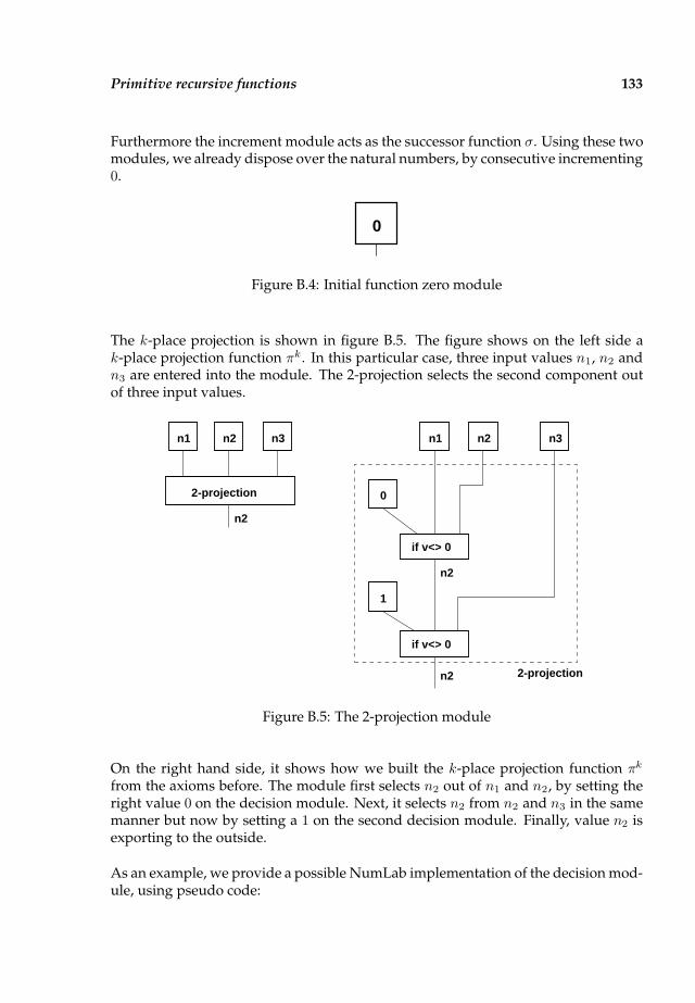
Primitive recursive functions 133
Furthermore the increment module acts as the successor function σ. Using these twomodules, we already dispose over the natural numbers, by consecutive incrementing0.
0
Figure B.4: Initial function zero module
The k-place projection is shown in figure B.5. The figure shows on the left side ak-place projection function πk. In this particular case, three input values n1, n2 andn3 are entered into the module. The 2-projection selects the second component outof three input values.
n1 n2 n3n2 n3n1
2-projection
n2
0
1
if v<> 0
if v<> 0
n2 2-projection
n2
Figure B.5: The 2-projection module
On the right hand side, it shows how we built the k-place projection function πk
from the axioms before. The module first selects n2 out of n1 and n2, by setting theright value 0 on the decision module. Next, it selects n2 from n2 and n3 in the samemanner but now by setting a 1 on the second decision module. Finally, value n2 isexporting to the outside.
As an example, we provide a possible NumLab implementation of the decision mod-ule, using pseudo code:
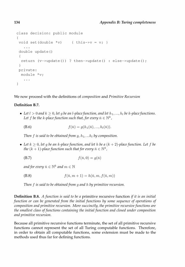
134 Appendix B: Turing completeness
class decision: public modulevoid set(double *v) this->v = v;
...double update()return (v->update()) ? then->update() : else->update();
private:module *v;...
We now proceed with the definitions of composition and Primitive Recursion
Definition B.7.
• Let l > 0 and k ≥ 0, let g be an l-place function, and let h1, ..., hl be k-place functions.Let f be the k-place function such that, for every n ∈ Nk,
(B.6) f(n) = g(h1(n), ..., hl(n)).
Then f is said to be obtained from g, h1, ...hl by composition.
• Let k ≥ 0, let g be an k-place function, and let h be a (k + 2)-place function. Let f bethe (k + 1)-place function such that for every n ∈ Nk,
(B.7) f(n, 0) = g(n)
and for every n ∈ Nk and m ∈ N
(B.8) f(n,m+ 1) = h(n,m, f(n,m))
Then f is said to be obtained from g and h by primitive recursion.
Definition B.8. A function is said to be a primitive recursive function if it is an initialfunction or can be generated from the initial functions by some sequence of operations ofcomposition and primitive recursion. More succinctly, the primitive recursive functions arethe smallest class of functions containing the initial function and closed under compositionand primitive recursion.
Because all primitive recursive functions terminate, the set of all primitive recursivefunctions cannot represent the set of all Turing computable functions. Therefore,in order to obtain all computable functions, some extension must be made to themethods used thus far for defining functions.
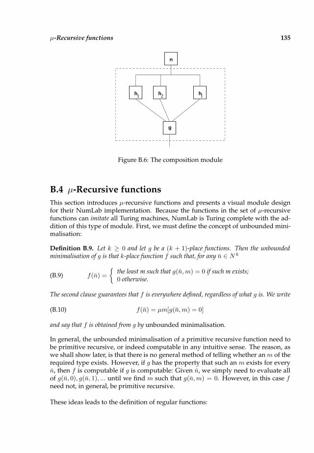
µ-Recursive functions 135
g
h1 h2 hl
n
Figure B.6: The composition module
B.4 µ-Recursive functions
This section introduces µ-recursive functions and presents a visual module designfor their NumLab implementation. Because the functions in the set of µ-recursivefunctions can imitate all Turing machines, NumLab is Turing complete with the ad-dition of this type of module. First, we must define the concept of unbounded mini-malisation:
Definition B.9. Let k ≥ 0 and let g be a (k + 1)-place functions. Then the unboundedminimalisation of g is that k-place function f such that, for any n ∈ N k
(B.9) f(n) =
the least m such that g(n,m) = 0 if such m exists;0 otherwise.
The second clause guarantees that f is everywhere defined, regardless of what g is. We write
(B.10) f(n) = µm[g(n,m) = 0]
and say that f is obtained from g by unbounded minimalisation.
In general, the unbounded minimalisation of a primitive recursive function need tobe primitive recursive, or indeed computable in any intuitive sense. The reason, aswe shall show later, is that there is no general method of telling whether an m of therequired type exists. However, if g has the property that such an m exists for everyn, then f is computable if g is computable: Given n, we simply need to evaluate allof g(n, 0), g(n, 1), ... until we find m such that g(n,m) = 0. However, in this case fneed not, in general, be primitive recursive.
These ideas leads to the definition of regular functions:
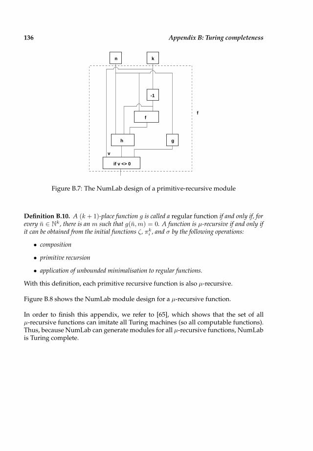
136 Appendix B: Turing completeness
-1
h
f
n k
g
f
if v <> 0
v
Figure B.7: The NumLab design of a primitive-recursive module
Definition B.10. A (k + 1)-place function g is called a regular function if and only if, forevery n ∈ Nk, there is an m such that g(n,m) = 0. A function is µ-recursive if and only ifit can be obtained from the initial functions ζ, πki , and σ by the following operations:
• composition
• primitive recursion
• application of unbounded minimalisation to regular functions.
With this definition, each primitive recursive function is also µ-recursive.
Figure B.8 shows the NumLab module design for a µ-recursive function.
In order to finish this appendix, we refer to [65], which shows that the set of allµ-recursive functions can imitate all Turing machines (so all computable functions).Thus, because NumLab can generate modules for all µ-recursive functions, NumLabis Turing complete.
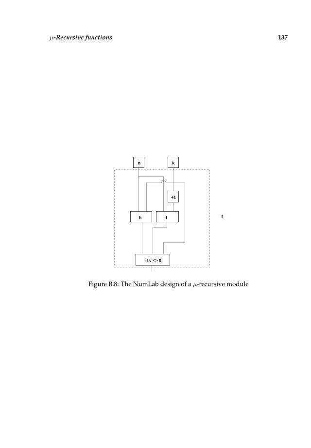
µ-Recursive functions 137
f
n k
h
if v <> 0
+1
f
Figure B.8: The NumLab design of a µ-recursive module


Bibliography
[1] G. Abram and L. Treinis. An extended data-flow architecture for data analysisand visualization. In Proc. IEEE Visualization, pages 263–270. ACM Press, 1995.
[2] E. Anderson, Z. Bai, and C. Bischof et al. LAPACK user’s guide. SIAM, Philadel-phia, 1995.
[3] P. Astheimer. Sonification tools to supplement dataflow visualization. ScientificVisualization: Advances and Challenges, pages 251–263, 1994.
[4] O. Axelsson. Iterative Solution Methods. Cambridge University Press, 1996.
[5] O. Axelsson and V. Barker. Finite Element Solution of Boundary Value Problems.Theory and Computation. Academic Press, Orlando, Florida, 1984.
[6] O. Axelsson and J. M. L. Maubach. Global space-time finite element methodsfor time-dependent convection diffusion problems. Advances in Optimizationand Numerical Analysis, 275:165–184, 1994.
[7] O. Axelsson and P. S. Vassilevski. Algebraic multilevel preconditioning meth-ods. I. Numerische Mathematik, 56:157–177, 1989.
[8] O. Axelsson and P. S. Vassilevski. Algebraic multilevel preconditioning meth-ods. II. SIAM Journal on Numerical Analysis, 27:1569–1590, 1990.
[9] R. Barrett, M. Berry, T. Chan, J. Demmel, J. Donato, J. Dongarra, V. Eijkhout,R. Pozo, C. Romine, and H. A. van der Vorst. Templates for the solution of linearsystems: Building blocks for iterative methods. SIAM, Philadelphia, 1994.
[10] F. L. Bauer. Optimally scaled matrices. Numerische Mathematik, 5:73–87, 1963.
[11] J. Bear and Y. Bachmat. Introduction of modelling of transport phenomena in porousmedia, Vol. 4. Kluwer, Dordrecht, 1990.
[12] M. W. Benson and P. O. Frederickson. Iterative solution of large sparse linearsystems arising in certain multidimensional approximation problems. UtilitasMathematica, 22:127–140, 1982.
[13] M. Benzi, J. K. Collum, and M. Tuma. Robust appoximate inverse precondi-tioning for the conjugate gradient method. SIAM Journal on Scientific Comput-ing, 22:1318–1332, 2000.

140 Bibliography
[14] M. Benzi, C. D. Meyer, and M. Tuma. A sparse approximate inverse precondi-tioner for the conjugate gradient method. SIAM Journal on Scientific Computing,17:1135–1149, 1996.
[15] M. Benzi and M. Tuma. Numerical experiments with two approximate inversepreconditioners. BIT, 38:234–241, 1998.
[16] M. Benzi and M. Tuma. A sparse approximate inverse preconditioner for non-symmetric linear systems. SIAM Journal on Scientific Computing, 19:968–994,1998.
[17] M. Benzi and M. Tuma. A comparative study of sparse approximate inversepreconditioners. Applied Numerical Mathematics, 30:305–340, 1999.
[18] G. Booch. Object-Oriented Analysis and Design, second edition. Ben-jamin/Cummings, Redwood City, CA, 1994.
[19] F. Bornemann and H. Yserentant. A basic norm equivalence for the theory ofmultilevel methods. Numerische Mathematik, 64:455–476, 1993.
[20] A. Bottcher and B. Silbermann. Introduction to large truncated Toeplitz matrices.Springer, New York, 1999.
[21] J. H. Bramble, D. Y. Kwak, and J. E. Pasciak. Uniform convergence of multigridv-cycle iterations for indefinite and nonsymmetric problems. SIAM Journal onNumerical Analysis, 31:1746–1763, 1994.
[22] J. H. Bramble, J. E. Pasciak, and A. H. Schatz. The construction of precondi-tioners for elliptic problems by substructuring, I. Mathematics of Computation,47:103–134, 1986.
[23] J. H. Bramble, J. E. Pasciak, and J. Xu. The analysis of multigrid algorithms fornonsymmetric and indefinite elliptic problems. Mathematics of Computation,51:389–414, 1988.
[24] J. H. Bramble, J. E. Pasciak, and J. Xu. Parallel multilevel preconditioners.Mathematics of Computation, 55:1–22, 1990.
[25] W. L. Briggs. A Multigrid Tutorial. SIAM, Philadelphia, 1987.
[26] A. M. Bruaset and H. P. Langtangen. A Comprehensive Set of Tools for SolvingPartial Differential Equations: Diffpack. 1996.
[27] R. Brun, M. Goto, and F. Rademakers. The cint c/c++ interpreter.http://root.cern.ch/root/CintInterpreter.html.
[28] T. Budd. An Introduction to Object-Oriented Programming. Addison-Wesley,1997.
Bibliography 141
[29] J. P. E. Buskens and M. J. D. Slob. Prototype of the Numlab program. A lab-oratory for numerical engineering. internal report RANA 96-04, EindhovenUniversity of Technology, Eindhoven, 1996.
[30] J. C. Butcher. The numerical analysis of ordinary differential equations : Runge-Kuttaand general linear methods. Wiley, 1987.
[31] T. C. Chan and H. A. van der Vorst. Approximate and Incomplete Factoriza-tions. In D. E. Keys, A. Samed, and V. Venkatakrishnan, editors, Parallel Nu-merical Algorithms, volume 4 of ICASE/LaRC Interdisciplinary Series in Scienceand Engineering, pages 167–202, Dordrecht, 1997. Kluwer Academic.
[32] Z. Chen and D. Y. Kwak. ν-cycle Galerkin-multigrid methods for nonconform-ing methods for nonsymmetric and indefinite problems. Applied NumericalMathematics, 28:17–35, 1998.
[33] Z. Chen, D. Y. Kwak, and Y. J. Yon. Multigrid algorithms for nonconformingand mixed methods for nonsymmetric and indefinite problems. SIAM Journalon Scientific Computing, 19:502–515, 1998.
[34] J. D. F. Cosgrove, J. C. Dıaz, and A. Griewank. Approximate inverse precondi-tionings for sparse linear systems. International Journal of Computer Mathemat-ics, 44:91–110, 1992.
[35] W. Dahmen and A. Kunoth. Multilevel preconditioning. Numerische Mathe-matik, 63:315–344, 1992.
[36] R. S. Dembo, S. C. Eisenstat, and T. Steihaug. Inexact newton methods. SIAMJournal on Numerical Analysis, 19:400–408, 1982.
[37] A. M. Duclos and M. Grave. Reference models and formal specification forscientific visualization. Scientific Visualization: Advances and Challenges, pages251–263, 1994.
[38] I. S. Duff and G. A. Meurant. The effect of ordering on preconditioned conju-gate gradients. BIT, 29:635–657, 1989.
[39] I. S. Duff and H. A. van der Vorst. Developments and trends in the parallelsolution of linear systems. Parallel Computing, 25:1931–1970, 1999.
[40] S. C. Eisenstat and H. F. Walker. Globally convergent inexact Newton methods.SIAM Journal on Optimization, 4:393–422, 1994.
[41] R. E. Ewing, S. I. Petrova, and P. S. Vassilevski. Two-level local refinement pre-conditioners for nonsymmetric and indefinite elliptic problems. SIAM Journalon Scientific Computing, 15:149–163, 1994.
[42] I. Fried. The l2 and l∞ condition numbers of the finite element stiffness andmass matrices, and the pointwise convergence of the method. In J.R. White-man, editor, The Mathematics of Finite Elements and Applications, pages 163–174,New York, 1973. Academic Press.

142 Bibliography
[43] I. Fried. Numerical Solution of Differential Equations. Academic Press, New York,1979.
[44] C. W. Gear. Numerical initial value problems in ordinary differential equations.Prentice-Hall, 1971.
[45] A. George and J. Liu. Computer solution of large sparse positive definite systems.Prentice Hall, Englewood Cliffs, New Jersey, 1981.
[46] J. R. Gilbert, C. Moler, and R. Schreiber. Sparse Matrices in MATLAB: Designand Implementation. SIAM Journal on Matrix Analysis and Application, 13:333–356, 1992.
[47] M. J. Grote and T. Huckle. Parallel preconditioning with sparse approximateinverses. SIAM Journal on Scientific Computing, 18:838–853, 1997.
[48] C. Gunn, A. Ortmann, U. Pinkall, K. Polthier, and U. Schwarz. Oor-ange: A Virtual Laboratory for Experimental Mathematics. Techni-cal Report Sonderforschungsbereich 288, Technical University Berlin.http://www-sfb288.math.tu-berlin.de/oorange/Oorange-Doc.html.
[49] I. Gustafsson. A class of first order factorization methods. BIT, 18:142–156,1978.
[50] M. A. Halse. IRIS Explorer User’s Guide. Silicon Graphics Inc., Mountain View,California, 1993.
[51] M. R. Hestenes and E. Stiefel. Methods of conjugate gradients for solving linearsystems. Journal of Research of the National Bureau of Standards. Sect. B, 49:409–436, 1952.
[52] W. D. Hoskings and G. E. McMaster. Band with five toeplitz matrices. Linearand Multilinear Algebra, 6:153 – 156, 1978.
[53] IMSL. FORTRAN Subroutines for Mathematical Applications, User’s Manual.IMSL, 1987.
[54] INRIA-Rocquencourt. Scilab Documentation for release 2.4.1. 2000.http://www-rocq.inria.fr/scilab/doc.html.
[55] N. Jackie, T. Davis, and M. Woo. OpenGL Programming Guide. Addison-Wesley,1993.
[56] B. Joe. Construction of a k-dimensional Delaunay triangulation using localtransformations. SIAM Journal on Scientific Computing, 14:1415–1436, 1993.
[57] V. John, J. M. L. Maubach, and L. Tobiska. A non-conforming streamline dif-fusion finite element method for convection diffusion problems. NumerischeMathematik, 78:165–188, 1997.

Bibliography 143
[58] R. E. Kaasschieter. A general finite element preconditioning for the conjugategradient mathod. BIT, 29:824–849, 1989.
[59] A. A. J. Ketelaars. Drying deformable media. Kinetics, shrinkage and stresses. PhDthesis, Eindhoven University of Technology, Eindhoven, 1992.
[60] L. Yu. Kolotilina and A. Yu. Yeremin. Factorized sparse approximate inversepreconditioning i: Theory. SIAM Journal onf Matrix Analysis and Applications,14:45–58, 1993.
[61] W. Kortsmit. NUMerical LABoratory uitbreidingen en iteratieve methoden.Master’s thesis, Eindhoven University of Technology, 1997.
[62] B. Kroes. The influence of material properties on drying kinetics. PhD thesis, Eind-hoven University of Technology, Eindhoven, 1999.
[63] C. Lartigue, J. R. Puiggali, and M. Quitard. A simplified study of moisturetransport in wood. In A. S. Mujamdar and M. A. Roques, editors, Drying ’89,pages 169–179. Hemisphere, 1989.
[64] W. Layton, J. M. L. Maubach, and P. Rabier. Parallel algorithms for maximalmonotone operators of local type. Numerische Mathematik, 71:29–58, 1995.
[65] H. R. Lewis and C. H. Papadimitriou. Elements of the Theory of Computation.Prentice-Hall, International (UK) Limited, London, 1981.
[66] S. D. Margenov and J. M. L. Maubach. Optimal algebraic multilevel precondi-tioning for local refinement along a line. Numerical Linear Algebra with Applica-tions, 2:347–361, 1995.
[67] Matlab. Matlab Reference Guide. The Math Works Inc., 1992.
[68] R. M. M. Mattheij and J. Molenaar. Ordinary differential equations in theory andpractice. Wiley, 1996.
[69] R. M. M. Mattheij and M. D. Smooke. Estimates for the inverse of tridiagonalmatrices arising in boundary-value problems. Linear Algebra and its Applica-tions, 73:33–57, 1986.
[70] J. M. L. Maubach. Local bisection refinement for n-simplicial grids generatedby reflections. SIAM Journal on Scientific Computing, 16:210–227, 1995.
[71] J. M. L. Maubach and W. D. Drenth. Data-flow oriented visual programminglibraries for scientific computing. In P.M.A. Sloot, C.J.K. Tan, J.J. Dongarra,and A.G. Hoekstra, editors, Computational Science – ICCS 2002 (LNCS 2329).Springer-Verlag, 2002.
[72] J. M. L. Maubach and A. C. Telea. Numerical laboratory for computation andvisualisation. Computing and Visualization in Science, accepted, 2001.
144 Bibliography
[73] J. M. L. Maubach and A. C. Telea. The numlab numerical laboratory for com-putational and visualisation. Computing and Visualisation in Science, 2003. ac-cepted.
[74] J. A. Meijerink and H. A. van der Vorst. An iterative solution method for linearsystems of which the coefficient matrix is a symmetric M-matrix. Mathematicsof Computation, 31:148–162, 1977.
[75] J. A. Meijerink and H. A. van der Vorst. Guidelines for the usage of incompletedeconpositions in solving sets of linear equations as they occur in practicalproblems. Journal of Computational Physics, 44:134–155, 1981.
[76] G. A. Meurant. Computer solution of the large linear systems. Elsevier NorthHolland, Amsterdam, 1999.
[77] B. Meyer. Object-oriented software construction. Prentice Hall, 1997.
[78] M. Magolu monga Made and H. A. van der Vorst. ParIC: A family of par-allel incomplete Cholesky preconditioners. In M. Bubak, H. Afsarmanesh,R. Williams, and B. Hertzberger, editors, High Performance Computing and Net-working, 8th International Conference, pages 89–98, Berlin, 2000. Springer Verlag.
[79] NAG. FORTRAN Library, Introductory Guide, Mark 14. Numerical AnalysisGroup Limited and Inc.,, 1990.
[80] D. M. Newitt and M. Coleman. The mechanisms of drying of solids. Part 3, thedrying characteristics of china clay. Transactions of the Institution of ChemicalEngineers, 30:28–45, 1952.
[81] M. Pastrnak. Distributed Visualisation and Simulation with Object-Oriented Net-works. PhD thesis, Eindhoven University of Technology, Eindhoven, 2002.
[82] W. Ribarsky, B. Brown, T. Myerson, R. Feldmann, S. Smith, and L. Treinish.Object-oriented, dataflow visualization systems - a paradigm shift? ScientificVisualization: Advances and Challenges, pages 251–263, 1994.
[83] J. Rumbaugh, M. Blaha, W. Premerlani, F. Eddy, and W. Lorensen. Object-Oriented Modelling and Design. Prentice-Hall, 1991.
[84] Y. Saad. Iterative Methods for Sparse Linear Systems. PWS publishing company,Boston, 1996.
[85] Y. Saad. SPARSEKIT: A basic toolkit for sparse matrix computations (Ver-sion 2). http://www.cs.umn.edu/research/arpa/SPARSKIT/sparskit.html,Boston, 1996.
[86] Y. Saad and M. H. Schulz. GMRES: a generalized minimal residual algorithmfor solving nonsymmetric linear systems. SIAM Journal on Scientific and Statis-tical Computing, 7:856–869, 1986.
Bibliography 145
[87] W. Schroeder, K. Martin, and B. Lorensen. The Visualization Toolkit: An Object-Oriented Approach to 3D Graphics. Prentice Hall, 1995.
[88] Y. Shapira. Multigrid methods for 3-D definite and indefinite problems. Ap-plied Numerical Mathematics, 26:377–398, 1998.
[89] P. Sonneveld. CGS, a fast Lanczos-type solver for nonsymmetric linear sys-tems. SIAM Journal on Scientific and Statistical Computing, 10:36–52, 1989.
[90] R. Stevenson. Modified ILU as a smoother. Numerische Mathematik, 68:295–309,1994.
[91] B. Stroustrup. The C++ Programming Manual (3rd edition). Addison-Wesley,1997.
[92] A. C. Telea. Combining Object Orientation and Dataflow Modeling in the Vis-sion Simulation System. In R. Mitchell, A. C. Wills, J. Bosch, and B. Meyer, ed-itors, Proceedings of TOOLS’99 Europe, Nancy 3-8 June 1999, pages 56–65. IEEEComputer Society Press, 1999.
[93] A. C. Telea. Visualisation and Simulation with Object-Oriented Networks. PhDthesis, Eindhoven University of Technology, Eindhoven, 2001.
[94] A. C. Telea and J. J. van Wijk. Vission: An Object Oriented dataflow system forsimulation and visualization. In E. Groeller and W. Ribarsky, editors, Proceed-ings of IEEE VisSym ’99, pages 95–104. Springer, 1999.
[95] W. F. Tinney and J. W. Walker. Direct solutions of sparse network equations byoptimally ordered triangular factorization. Proceedings of IEEE, 55:1801–1809,1967.
[96] M. J. Todd. The Computation of Fixed Points and Applications, Lecture Notes inEconomics and Mathematical Systems 124. Springer Verlag, 1976.
[97] C. Upson, T. Faulhaber, D. Kamins, D. Laidlaw, D. Schlegel, J. Vroom, R. Gur-witz, and A. van Dam. The application visualization system: A computationalenvironment for scientific visualization. IEEE Computer Graphics and Applica-tions, pages 30–42, 1989. See also http://www.avs.com.
[98] A. van der Sluis. Condition numbers and equilibration of matrices. NumerischeMathematik, 14:14–23, 1969.
[99] A. van der Sluis. Condition, equilibration and pivoting in linear algebraicsystems. Numerische Mathematik, 15:74–86, 1970.
[100] A. van der Sluis. Stability of solutions of linear algebraic systems. NumerischeMathematik, 14:246–251, 1970.
[101] H. A. van der Vorst. High performance preconditioning. SIAM Journal onScientific and Statistical Computing, 10:1174–1185, 1989.
146 Bibliography
[102] H. A. van der Vorst. Bi-CGSTAB: a fast and smoothly converging variant of Bi-CG for the solution of nonsymmetric linear systems. SIAM Journal on Scientificand Statistical Computing, 13:631–644, 1992.
[103] H. A. van der Vorst. Iterative Krylov Methods for Large Linear Systems. Cam-bridge Monographs on Applied and Computational Mathematrics. Cam-bridge University Press, 2003.
[104] H. A. van der Vorst and K. Dekker. Conjugate gradient type methods andpreconditioning. Journal of Computational and Applied Mathematics, 24:73–87,1988.
[105] J. Wernecke. The Inventor Mentor: Programming Object-Oriented 3D Graphicswith Open Inventor. Addison-Wesley, 1993.
[106] G. Wittum. On the robustness of ILU smoothing. SIAM Journal on Scientific andStatistical Computing, 10:699–717, 1989.
[107] S. Wolfram. The Mathematica Book 4-th edition. Cambridge University Press,1999.
[108] Y. J. Yon and D. Y. Kwak. Nonconforming multigrid methid for nonsymmetricand indefinite problems. Computers & Mathematics with Applications, 30:1–7,1995.
Index
alphabet . . . . . . . . . . . . . . . . . . . . . . . . . 129AMLI . . . . . . . . . . . . . . . . . . . . . . . . . . . . . 33approximate inverse . . . . . . . . . . . . . . . 35
AINV . . . . . . . . . . . . . . . . . . . . . . . . . 37Frobenius norm minimization.35FSAI . . . . . . . . . . . . . . . . . . . . . . . . . . 37SPAI . . . . . . . . . . . . . . . . . . . . . . . . . . 36
Bi-CG . . . . . . . . . . . . . . . . . . . . . . . . . . . . . 25blank symbol . . . . . . . . . . . . . . . . . . . . .130BPX . . . . . . . . . . . . . . . . . . . . . . . . . . . . . . . 33
CG . . . . . . . . . . . . . . . . . . . . . . . . . . . . . . . . 25CGS . . . . . . . . . . . . . . . . . . . . . . . . . . . . . . . 26Church’s Thesis . . . . . . . . . . . . . . . . . . 131Church-Turing’s Thesis . . . . . . . . . . . 131composition . . . . . . . . . . . . . . . . . . . . . . 134computational complexity . . . . . . . . . 27control unit . . . . . . . . . . . . . . . . . . . . . . 129
diagonally oriented grid . . . . . . . . . . . 71
equilibration . . . . . . . . . . . . . . . . . . . . . . 39
fill-in path . . . . . . . . . . . . . . . . . . . . . . . . . 12finite-state machine . . . . . . . . . . . . . . 129flops . . . . . . . . . . . . . . . . . . . . . . . . . . . . . . 27
Green’s functions . . . . . . . . . . . . . . . . . . 35Green’s matrix . . . . . . . . . . . . . . . . . . . . 35
halt state . . . . . . . . . . . . . . . . . . . . . . . . . 131
imitate . . . . . . . . . . . . . . . . . . . . . . . . . . . 135incomplete factorizations . . . . . . . . . . 34iterative methods
Bi-CG. . . . . . . . . . . . . . . . . . . . . . . . .25
CG . . . . . . . . . . . . . . . . . . . . . . . . . . . 25CGS . . . . . . . . . . . . . . . . . . . . . . . . . . 26SOR . . . . . . . . . . . . . . . . . . . . . . . . . . 24
Jacobi matrix . . . . . . . . . . . . . . . . . . . . . . 24
Krylov subspace. . . . . . . . . . . . . . . . . . .25Krylov subspace method . . . . . . . . . . 25
language . . . . . . . . . . . . . . . . . . . . . . . . . 129Left-right (LR) ordering . . . . . . . . . . . 10
maximal monotone . . . . . . . . . . . . . . . . 89Minimum degree ordering . . . . . . . . 10multigrid . . . . . . . . . . . . . . . . . . . . . . . . . . 33
network editor . . . . . . . . . . . . . . . . . . . . . 3nonstationary iterative methods . . . 23
optimal order method . . . . . . . . . . . . . 28
preconditionersAMLI . . . . . . . . . . . . . . . . . . . . . . . . . 33BPS . . . . . . . . . . . . . . . . . . . . . . . . . . . 34BPX . . . . . . . . . . . . . . . . . . . . . . . . . . 33incomplete factorizations . . . . . 34multigrid . . . . . . . . . . . . . . . . . . . . . 33
preconditioning . . . . . . . . . . . . . . . . 27, 31explicit . . . . . . . . . . . . . . . . . . . . . . . 32implicit . . . . . . . . . . . . . . . . . . . . . . . 32
Primitive Recursion . . . . . . . . . . . . . . 134primitive recursive function . . . . . . 134
regular function . . . . . . . . . . . . . . . . . . 136residual . . . . . . . . . . . . . . . . . . . . . . . . . . . 23Reverse Cuthill-McKee ordering . . . 10Ritz-Galerkin approach . . . . . . . . . . . . 25
148 Index
SOR . . . . . . . . . . . . . . . . . . . . . . . . . . . . . . . 24spectral condition number . . . . . . . . . 25spectral radius . . . . . . . . . . . . . . . . . . . . 24stationary iterative methods . . . . . . . 23string . . . . . . . . . . . . . . . . . . . . . . . . . . . . 129suboptimal order method . . . . . . . . . 28
tape . . . . . . . . . . . . . . . . . . . . . . . . . . . . . . 129tie-breaking strategy . . . . . . . . . . . . . . . . 8Toeplitz matrix . . . . . . . . . . . . . . . . . . . . 45total workload . . . . . . . . . . . . . . . . . . . . 27Turing complete . . . . . . . . . . . . . . . . . . 131Turing machine . . . . . . . . . . . . . . . . . . 129
unbounded minimalisation . . . . . . . 135
visualizationsteering . . . . . . . . . . . . . . . . . . . . . . . . 1tracking and monitoring . . . . . . . 1

Summary
Often solving partial differential equations in engineering and sciences is compli-cated by the fact that their solutions exhibit sharp peaks or fronts. Any suitable dis-cretization method for numerically solving such problems should use a grid takingthis activity into account. As a result the mesh is usually quite far from being uni-form. This in turn causes difficulties when solving the linear systems that arise fromsuch discretized problems; often as a step in a Newton process when the problemat hand is non-linear. The resulting system is said to be ill-conditioned. Typicallythe solution is found by an iterative method. If the problem is ill-conditioned theconvergence (if at all) will be slow.In order to speed up convergence so called preconditioning techniques are widelyused. We consider a class of problems, related to moisture and salt ion transporta-tion in a brick wall, for which no effective preconditioner exists as of yet. This thengives the first objective of this thesis: to construct techniques that are able to tacklethis problem. A first approach is based on Gaussian elimination for a particularnumbering scheme for the degrees of freedom related to refinement along a line.Secondly we consider preconditioning techniques based on approximating the in-verse. The advantage of this type of preconditioning is that application requiresonly matrix-vector multiplications. More importantly, for the problem above men-tioned standard preconditioning techniques based on incomplete factorizations areprone to break down. For this approximate inverse preconditioner we derive sev-eral estimates for the spectral condition number in the one dimensional case. Thisanalysis is based on a slightly modified variant so that Toeplitz matrix theory can beused. A further analysis of this preconditioner shows that the degrees of freedomdecouple into two sets. In the one dimensional case we derive an algorithm basedon recursive application of this decoupling after applying this approximate inversepreconditioner. For two dimensions this cannot be generalized straightforwardlyand we provide suggestions for a recursive application of the approximate inverse.
Besides the need for efficient solvers, another important aspect is to have a computa-tional platform to run those solvers and perform numerical simulations. This is oursecond objective. A suitable computational platform should enable the researcherto use existing software and offer the possibility to extend the platform with newlymade software components for future use. Furthermore, there should be the possi-bility to track and steer the simulation at runtime. This thesis describes the so calledNumLab environment that enables the researcher to implement and test new ideas

150 Summary
by reusing existing components and building new components from scratch or fromexisting components. Mathematical concepts like operators and linear solvers areimplemented using a generic interface, which enables interactive change of compo-nents and parameters.
We illustrate the foregoing by a series of numerical examples. The approximate in-verse preconditioner is tested using the NumLab environment. The numericallycomputed spectral condition numbers turn out to agree nicely with the theoreticalestimates. To illustrate the robustness our results are compared to an incompletefactorization preconditioner. The latter breaks down, as does the iterative solver ap-plied to the linear system of equations without preconditioning.
Samenvatting
Het oplossen van partiele differentiaalvergelijkingen uit technische en wetenschap-pelijke toepassingen wordt vaak bemoeilijkt doordat de oplossingen op bepaaldegebieden scherpe pieken of fronts vertonen. Elke geschikte discretisatiemethode omzulke problemen numeriek op te lossen, behoort daartoe een rekenrooster te kie-zen dat deze kenmerken in ogenschouw neemt. Als gevolg hiervan is het roosterdoorgaans verre van uniform. Dit op zijn beurt geeft moeilijkheden wanneer het li-neaire stelsel dat volgt uit de discretisatie opgelost moet worden; vaak als stap in eenNewton proces als het probleem in kwestie niet-lineair is. Het resulterende systeemwordt dan ook wel slecht geconditioneerd genoemd. In het algemeen wordt de op-lossing gevonden met behulp van een iteratieve methode. Als het probleem slechtgeconditioneerd is, dan zal de convergentie (zo die er al is) traag zijn.Om de convergentie te versnellen wordt veelvuldig gebruikt gemaakt van zoge-naamde preconditioneringstechnieken. Wij bekijken een klasse van problemen, ge-relateerd aan vocht- en zouttransport in een muur van bakstenen, waarvoor op ditmoment nog geen effectieve preconditioneerder bestaat. Dit geeft het eerste doelvan dit proefschrift: het construeren van technieken die in staat zijn deze problemenaan te pakken. Een eerste aanpak is gebaseerd op Gauss eliminatie voor een speci-fieke nummering van de onbekenden die bij een verfijning langs een lijn horen. Tentweede bekijken we preconditioneringstechnieken die gebaseerd zijn op het bena-deren van de inverse. Het voordeel van dit type preconditioneerders is dat de toe-passing ervan alleen matrix-vector vermenigvuldigingen vereist. Nog belangrijkeris dat voor het bovengenoemde probleem standaard preconditioneringstechniekengebaseerd op onvolledige factorisatie de neiging tot mislukken hebben. Voor dezebenaderde inverse preconditioneerder leiden we voor het een dimensionale gevalenkele schattingen voor het spectrale conditiegetal af. Deze analyse maakt gebruikvan een gedeeltelijk aangepaste variant opdat Toeplitz matrixtheorie toegepast kanworden. Verdere bestudering van deze preconditioneerder leert dat de onbekendenontkoppelen in twee verzamelingen. We leiden voor het eendimensionale geval eenalgortime af dat gebruik maakt van het recursief toepassingen van deze ontkoppe-ling na toepassing van de benaderde inverse preconditioneerder. In twee dimensiesin dit niet rechtstreeks generaliseerbaar. We geven enkele voorstellen voor het recur-sief gebruik van de benaderde inverse.
Naast de behoefte aan efficiente oplosmethoden is het hebben van een rekenplatformvoor het gebruiken van die oplosmethoden en het uitvoeren van numerieke simu-
152 Samenvatting
latie een ander belangrijk aspect. Dit is ons tweede doel. Een geschikt rekenplat-form zou de onderzoeker in staat moeten stellen om bestaande programmatuur tegebruiken en nieuw ontwikkelde programmatuur voor toekomstig gebruik aan hetplatform toe te voegen. Verder moet er ook de beschikking zijn over middelen omde simulatie te volgen en te sturen terwijl deze loopt. Dit proefschrift beschrijft dezogeheten NumLab-omgeving die de onderzoeker in staat stelt om nieuwe ideeen teimplementeren en te testen door bestaande componenten te hergebruiken en nieuwecomponenten te bouwen uit het niets of uit bestaande delen. Wiskundige conceptenzoals operatoren en lineaire oplossers zijn geımplementeerd met gebruikmaking vaneen generieke interface. Dit staat het interactief veranderen van componenten en pa-rameters toe.
Het voorgaande illustreren we met een reeks numerieke voorbeelden. De bena-derde inverse preconditioneerder wordt getest met gebruikmaking van de NumLab-omgeving. De numeriek berekende spectrale conditiegetallen zijn goed in overeen-stemming met de theoretische schattingen. Om de robuustheid te illustreren verge-lijken we onze resultaten met een onvolledige factorizatie preconditioneerder. Delaatste blijkt niet robuust, net als de iteratieve oplosser toegepast op het ongeprecon-ditioneerde lineaire stelsel van vergelijkingen.
Curriculum Vitae
The author of this thesis was born on January 9th, 1976 in the city of Nijmegen. Thegreater part of his childhood was spent in Deest, a small village on the south bankof the river Waal between Nijmegen and Tiel. After elementary school he went tothe Pax Christi College in Druten in 1987 where he obtained his VWO diploma in1993. Following this pre-university education the author went to study mathematicsat the University of Nijmegen. He specialized in the subject of numerical analysis,with a strong component of functional analysis. He also followed several courses inLatin, and participated in a drama group called Moira. In June 1998 he finished hismaster’s thesis on the subject of least-squares methods for first order systems undersupervision of prof. Axelsson. On August 1st, 1998 he assumed a PhD position atEindhoven University of Technology in the Scientific Computing Group. Several re-sults of his research are written in this thesis. As part of this research the 7th CopperMountain Conference on Iterative Methods was attended in 2002.Next to being a mathematician, Drenth has a strong interest in historical matters aswell. This resulted in a cooperation with several others from around the world tostudy the history of the British Army. The author has a particular interest in thereserve forces of the British Army. His research in this field will result in a series ofbooks to be published from 2005 on.