A Physics-based Model for PEMFCs: Process Identification from EIS Simulation

Georg Futter1, Arnulf Latz1,2, Thomas Jahnke1

1: German Aerospace Center (DLR), Stuttgart, Germany

2: Helmholtz Institute Ulm for Electrochemical Energy Storage (HIU), Ulm, Germany

DLR.de • Chart 1

Why physical modeling of fuel cells? • Better understanding of processes in the cell and their interaction • Insights on experimentally inaccessible properties • Simulation based prediction of cell performance and lifetime • Optimization of cell performance and durability Challenges: • Complex system: coupling of processes on very different time and length

scales • Details of the involved mechanisms often unknown and material dependent • Heterogeneities within the cell require 2D and 3D cell models

Motivation

DLR.de • Chart 2

Modeling approach

DLR.de • Chart 3

Educt

Product

Educt

Product

CATHODE ANODE

Multi-scale cell models

Degradation models

Model validation

0.5 1.0 1.5 2.0 2.5 3.0-0.40.00.40.81.21.62.02.42.83.2

Radius / nm

100% ECSA 90% ECSA 80% ECSA

PSD

Framework

DLR.de • Chart 4

Neopard.FC/EL

Dumux

DUNE

Generic framework for the simulation of multi-phase flow and transport in porous media

Modular toolbox for solving partial differential equations (PDEs) with grid-based methods

Framework to investigate performance and degradation of fuel cells and electrolyzers via transient 2D and 3D simulations

cH2O / mol/m3

• Developed at DLR since 2013

NEOPARD-FC features • 2D and 3D discretizations of the cells • Transport models for the cell components • Electrochemistry models • Specific fluid systems for the different

technologies • Transient simulations (e.g. EIS) • Models for degradation mechanisms

Field of Application: • PEMFC • DMFC • SOEC

NEOPARD-FC/EL: Numerical Environment for the Optimization of Performance And Reduction of Degradation of Fuel Cells/ELectrolyzers

DLR.de • Chart 5

• 9 layers spatially resolved (channels, GDLs, MPLs, CLs, MEM)

• Two-phase multi-component transport model

• Charge transport in ionomer phase • Ionomer film model • ORR: BV kinetics with doubling of

Tafel slope • Platinum oxide model • Gas crossover through membrane • Non-isothermal • Realistic boundary conditions:

lambda-control at fixed back pressure in potentiostatic and galvanostatic mode

PEMFC model features

DLR.de • Chart 6

H2

O2

H2O

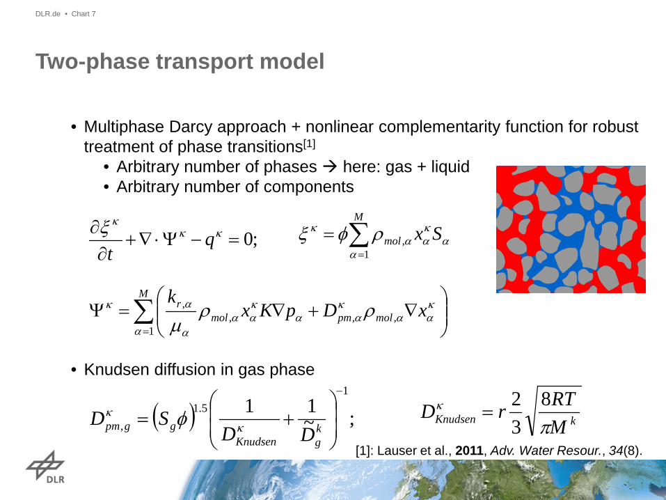
• Multiphase Darcy approach + nonlinear complementarity function for robust treatment of phase transitions[1]

• Arbitrary number of phases here: gas + liquid • Arbitrary number of components

• Knudsen diffusion in gas phase

Two-phase transport model

DLR.de • Chart 7

[1]: Lauser et al., 2011, Adv. Water Resour., 34(8).

;0=−Ψ⋅∇+∂∂ κκ

κξ qt

αα

καα

κ ρφξ SxM

mol∑=

=1

,

∑=

∇+∇=Ψ

M

molpmmolr xDpKx

k

1,,,

,

α

καα

καα

καα

α

ακ ρρµ

( ) ;~11

15.1

,

−

+= k

gKnudsenggpm DD

SD κκ φ kKnudsen M

RTrDπ

κ 832

=

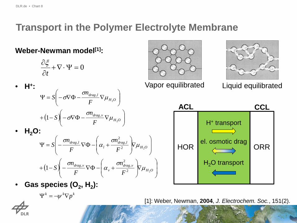
Weber-Newman model[1]: • H+: • H2O:

• Gas species (O2, H2):

Transport in the Polymer Electrolyte Membrane

DLR.de • Chart 8

[1]: Weber, Newman, 2004, J. Electrochem. Soc., 151(2).

0=Ψ⋅∇+∂∂

tξ

( )

∇−Φ∇−−+

∇−Φ∇−=Ψ

OHvdrag

OHldrag

Fn

S

Fn

S

2

2

,

,

1 µσ

σ

µσ

σ

( )

∇

+−Φ∇−−+

∇

+−Φ∇−=Ψ

OHvdrag

vvdrag

OHldrag

lldrag

Fn

Fn

S

Fn

Fn

S

2

2

2

2,,

2

2,,

1 µσ

ασ

µσ

ασ

ACL CCL

HOR ORR

H+ transport

el. osmotic drag

H2O transport

Vapor equilibrated Liquid equilibrated

kkk p∇−=Ψ ψ

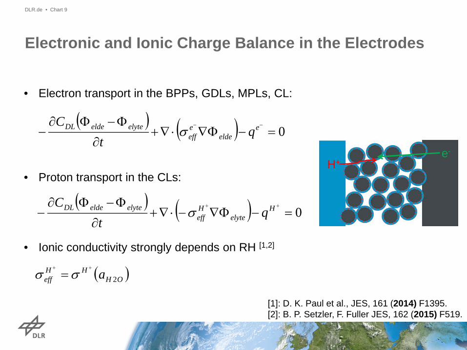
• Electron transport in the BPPs, GDLs, MPLs, CL: • Proton transport in the CLs: • Ionic conductivity strongly depends on RH [1,2]

Electronic and Ionic Charge Balance in the Electrodes

DLR.de • Chart 9

( ) ( ) 0=−Φ∇⋅∇+∂

Φ−Φ∂−

−− eelde

eeff

elyteeldeDL qt

Cσ

( ) ( ) 0=−Φ∇−⋅∇+∂

Φ−Φ∂−

++ Helyte

Heff

elyteeldeDL qt

Cσ

( )OHHH

eff a 2

++

= σσ

H+ e-

[1]: D. K. Paul et al., JES, 161 (2014) F1395. [2]: B. P. Setzler, F. Fuller JES, 162 (2015) F519.

• Model for ORR reaction rate taking into account • Oxygen transport through ionomer film • Resistances at gas/ionomer and ionomer/Pt interfaces[1]

• Analytical solutions are possible for and

• Reaction rate for :

Ionomer film model

DLR.de • Chart 10

[1]: Hao et al., JES, 162 (2015) F854.

O2

knFA

RkkRcFnAr

eff

Oeff

24 22

222 −+

=

−

−

= −

RTnF

RTnFciECSAk refo

ηαηα )1(expexp5.0

( )OHionO

ion aRD

R 2int,2

+=δ

2OBV cr ∝ 2OBV cr ∝

2OBV cr ∝

Model validation

DLR.de • Chart 11

• Model validation under various operating conditions is important for reliability

• Different RH

• Strong effect of RH on cell performance (Tafel slope + transport)

Model validation

DLR.de • Chart 12

• Model validation under various operating conditions is important for reliability

• Different RH • Different pressure

• Strong effect of RH on cell performance (Tafel slope + transport)

Model validation

DLR.de • Chart 13

• Model validation under various operating conditions is important for reliability

• Different RH • Different pressure • Different stoichiometry

• Strong effect of RH on cell

performance (Tafel slope + transport)

• High stoichiometry at 50% leads to lower performance drying out overcompensates higher oxygen partial pressure

Model validation

DLR.de • Chart 14

• Model validation under various operating conditions is important for reliability

• Different RH • Different pressure • Different stoichiometry

• Strong effect of RH on cell

performance (Tafel slope + transport)

• High stoichiometry at 50% leads to lower performance drying out overcompensates higher oxygen partial pressure

• 50% RH at 2 bar shows similar performance to 90% RH at 1.5 bar

Model validation

DLR.de • Chart 15

Impedance measurements at various current densities for 30% RH and 50% RH: • Trends and frequencies are correctly

described by the model • Total values still show a significant

deviation

• RH affects proton conductivity and gas transport through ionomer

• Inductive feature at low frequency can explain the difference between low frequency resistance and slope of iV-curve Ionic conductivity in CLs PtOx coverage Thermal effects

Cathode catalyst utilization

DLR.de • Chart 16

ORR reaction rate distribution • Location of maximum

reaction rate and distribution strongly depends on operating conditions

• At high RH • Very homogeneous at

low current densities

• At low RH • Strong heterogeneities

along channel • A significant part of the

CCL is not used

30%RH 90%RH

0.2A/cm2

0.6A/cm2

/ A/m3

/ A/m3

i / A/m2

i / A/m2

Chemical Membrane Degradation

DLR.de • Chart 17

O2 partial pressure / Pa

+−+ →+ 23 FeeFe

222 22 OHeHO →++ −+

[1]: Wong & Kjeang, 2015, Chem. Sus. Chem. 8(6).

Chemical Membrane Degradation

DLR.de • Chart 18

OCV 0.9 V 0.8 V cH2O2 / mol m-3

• O2 crossover governs the H2O2 formation at the anode maximum concentration on anode side at the cathode inlet

• At OCV: small gradients in electrolyte potential ions move due to concentration gradients

• Overpotential for reduction is highest at the anode

• At 0.8V: Increasing gradients in electrolyte potential drag the ions to the cathode side Degradation ceases

cFe2+ / mol m-3

Chemical Membrane Degradation

DLR.de • Chart 19

OCV 0.9 V 0.8 V Rate of SO3 group loss / mol m-3 s-1

• At OCV: Combination of H2O2 formation and transport with the Fe redox cycle leads to high degradation rate at the ACL / PEM interface until reinforcement layer consistent with experimental results

• Decreasing cell potential results in strongly reduced degradation

• Simulated fluorine emission rates are in good agreement with experimental data

Fluorine emission rate (FER) @ 95 °C, pAnode=2.5 bar, pCathode=2.3 bar, RH=75% (experiments provided by CEA)

• The development of predictive fuel cell models is challenging: • Complex interplay of many mechanisms on various time and length scales • Strong gradients within the cell require the development of 2D and 3D

models • Model validation has to be performed under various operating conditions,

ideally including the simulation of impedances to ensure model reliability • Current density distribution strongly depends on the operating conditions • At low relative humidity only a small fraction of the CL is used

• Chemical degradation of the membrane in PEMFC proceeds in several steps:

Oxygen crossover from cathode to anode Hydrogen peroxide formation Radical formation Radical attack of the membrane

• Amount and location of membrane degradation strongly depends on the cell potential. Highest degradation during OCV at anode side.

Summary

DLR.de • Chart 20

Thank you for your attention

The research leading to these results has received funding from the European Union's Seventh Framework Program (FP7/2007-2013) for the Fuel Cells and Hydrogen Joint Technology Initiative

under grant agreement n°256776, n°.303419 and n°621216

DLR.de • Chart 21

!Premium Act

"It can scarcely be denied that the supreme goal of all theory is to make the irreducible basic elements as simple and as few as possible without having to surrender the adequate representation of a single datum of experience“ Albert Einstein

Transport and Performance Model: Gases and Liquid

DLR.de • Chart 22

Two-phase transport of gases and liquid

NCP-equations for phase transitions[1]

• If a phase is not present:

• If a phase is present

[1]: Lauser et al., 2011, Adv. Water Resour., 34(8).

∑=

≤→=∀N

xS1

10:κ

κααα

01:1

≥→=∀ ∑=

ακ

καα Sx

N

01:1

=

−∀ ∑

=

N

xSκ

κααα

(1)

(2)

(3)

• Equations 1-3 constitute a non-linear complementarity problem

• Solution is a non-linear complementarity function:

( )000

0,=⋅∧≥∧≥

=Φbaba

ba

( )

−=Φ ∑=

N

xSba1

1,min,κ

καα

Liquid

Coupling Interface

Gas

PEM CL

Sol

id

Physical Coupling: • Macroscopic Approach: • Local thermodynamic equilibrium

Numerical Coupling: • Dirichlet-Neumann

Model Coupling and Schroeder’s Paradox

DLR.de • Chart 23

llggPEM SS λλλ +=

lS

lg SS −=1( )OHg af

2=λ

22≈lλ

Chemical Degradation Model

DLR.de • Chart 24

Fe redox cycle and transport • Electrochemical reaction:

• Description of ion transport in the membrane with generalized Nernst-Planck type equation[1]:

+−+ →+ 23 FeeFe

+=

+

+

2

3ln77.00Fe

Fe

cc

E

−−

= ++ RT

FRT

FccakFr FeFe 2exp

2exp32

ηη

elyteiiiiii FczucDJ Φ∇−∇−= RTufD iii =

[1]: Auclair et al., 2002, J. Memb. Sci., 195, 89–102.

36.0=+Naf

025.03/2 =+Fef

[1]

Value for bi/trivalent ions is expected to be lower:

Radical Formation Reactions

DLR.de • Chart 25

Nr. Reaction k (M-1 s-1) Eact (kJ mol-1)

1 Fe2+ + H2O2 + H+ → Fe3+ + HO• +H2O 65 35.4

2 Fe3+ + H2O2 → Fe2+ + HOO• + H+ 7·10-4 126

3 Fe2+ + HOO• + H+ → Fe3+ + H2O2 1.2·106 42

4 Fe3+ + HOO• → Fe2+ + O2 +H+ 2·104 33

5 HO• + H2O2 → HOO• + H2O 2.7·107 14

6 HOO• + H2O2 → HO• + H2O + O2 3 30

7 2HOO• → H2O2 + O2 8.6·105 (s-1) 20.6

8 HO• + H2 → H• + H2O 4.2·107 ???

9 H• + O2 → HOO• 2.1·1010 ???

[1]

[1]: Ghelichi et al., 2014, J. Phys. Chem. B, 118(38). [2]: Gubler et al., 2011, J. Electrochem. Soc., 158(7).

[2]

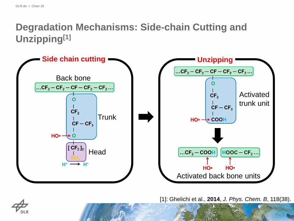
Degradation Mechanisms: Side-chain Cutting and Unzipping[1]

DLR.de • Chart 26

Back bone

Trunk

Head

Activated trunk unit

Activated back bone units

Side chain cutting Unzipping

[1]: Ghelichi et al., 2014, J. Phys. Chem. B, 118(38).

Degradation Reactions

DLR.de • Chart 27

Nr. Reaction k (M-1 s-1) Eact (kJ mol-1)

10 HO• + head group → products 3.7·106 ???

11 HO• + activated trunk unit → products 7.9·105 ≈70

12 HO• + activated back bone unit → products 7.9·105 ≈70 Unzipping

Side-chain cutting

Rate constants at room temperature: • Measured by: Dreizler & Roduner, 2012, Fuel Cells, 12(1). Activation energy for unzipping: • Estimated by: Gubler et al., 2011, J. Electrochem. Soc., 158(7).

• The loss of electrochemical active surface area (ECSA) at the cathode is mainly responsible for performance degradation

• Loss of ECSA is related to a growth of the platinum particles

• Different processes can contribute to the particle growth:

• Ostwald ripening • Coalescence

• Key property for mathematical desciption: particle size distribution (PSD) N(r)

• Balance equation for PSD

Catalyst degradation: Particle growth mechanism

DLR.de • Chart 28

CoalOstwald ttrN

trtrN

rttrN

δδ ),(),(),(

=

∂∂

∂∂

+∂

∂

Catalyst degradation: Coalescence mechanism

DLR.de • Chart 29

• Movement of the platinum particles on

the carbon support can lead to coalescence of the particles

• The coalescence can be described by an integro-differential equation for the particle distribution:

• Mechanisms for particle diffusion:

• (i) Ion attachment/detachment1: • (ii) Adatom diffusion2 (high temp.):

Coalescence of two particles to one with size r

Coalescence of a particle with size r

( ) drtrNtrNrDrDdrrr

trrNtrNrDrt

trN r

Coal∫∫∞

+−−−

=00

3/233

3/1332 ),'(),()'()('

)'(),)'((),'()'(),(

δδ

1~)( −rrD4~)( −rrD

[1]: S.V. Khare, N.C. Bartelt, T.L. Einstein, Physical Review Letters 75 (1995) 2148 [2]: F. Behafarid, B.R. Cuenya, Surface Science 606 (2012) 908

Catalyst degradation: Ostwald ripening

DLR.de • Chart 30

• Change of particle sizes due to Pt

dissolution and precipitation Pt Pt2+

+ 2 e– • The particle stability depends on the

particle size (surface energy):

• Experimental observation: Degradation is accelerated by cycling.

• Explanation: The formation and reduction of platinum oxides play an important role for the dissolution A model for the oxide formation is needed

rrGT

γµµµ Ω=∞−=∆

2)()(

Catalyst degradation: Effect of platinum oxides

DLR.de • Chart 31

• Simple platinum oxide model:

• Platinum oxides form a protective layer at high potentials, reducing the dissolution

Pt + H2O PtO + 2H+ + 2e- • At low potential the oxides are reduced • Going back to high potential leads to

accelerated dissolution until the protective layer is formed again

Pt Pt2+ + 2 e–

Fast degradation expected after sweep from low to high potential

Sweep to low potential

Sweep to high potential

Catalyst degradation: Effect of platinum oxides

DLR.de • Chart 32

• Recent experiments show that faster dissolution

occurs during sweep to low potentials [1] contradiction to simple model!

• Advanced model: • Include the place exchange between

platinum and oxygen atoms • Pt + H2O PtOsurf + 2H+ + 2e-

• PtOsurf PtObulk • PtObulk + H2O PtO2 + 2H+ + 2e-

• Dissolution occurs also during the place exchange accelerated degradation during sweep to low potentials

• PtObulk + 2 H+ Pt2+ + H2O

[1] A. A. Topalov et al., Chem. Sci. 5 (2014) 631

Catalyst degradation: Modeling the particle growth

DLR.de • Chart 33

• The particle growth mechanisms lead

to a change in the PSD and a loss of ECSA

• Time evolution of ECSA depends on the mechanism

0 100 200 300 400 500 600 700 800 90010000.4

0.6

0.8

1.0

Time / h

Experiment Simulation mechanism I Simulation mechanism II

ECSA

/ECS

A 0

Catalyst degradation: Modeling the particle growth

DLR.de • Chart 34

• The particle growth mechanisms lead

to a change in the PSD and a loss of ECSA

• Time evolution of ECSA depends on the mechanism

• The shape of the PSD also depends on the mechanism:

• Tail at small particle sizes is formed during Ostwald ripening

• Tail at large particle sizes and second peak is formed during coalescence

Analyzing the PSD (e.g. with transmission electron microscopy) can help identifying the relevant degradation mechanism

0.5 1.0 1.5 2.0 2.5 3.0-0.40.00.40.81.21.62.02.42.83.2

Radius / nm

100% ECSA 90% ECSA 80% ECSA

PSD

0.5 1.0 1.5 2.0 2.5 3.00.00.40.81.21.62.02.42.83.2

Radius / nm

100% ECSA 90% ECSA 80% ECSA

PSD

Ostwald ripening

Coalescence