112/04/20 1

A Particle-and-Density Based Evolutionary Clustering Method for

Dynamic Networks

Min-SooKim and Jiawei Han

Proceeding of the International Conference on Very Large Data Bases, VLDB, 2009

Speaker: Chien-Liang Wu

Outline Introduction Motivation & Goals Particle-and-Density Based Evolutionary Clustering

Modeling of Community Local Clustering Mapping of Local Clusters

Experiments Conclusions

2

Dynamic Networks Sequence of networks with different timestamps

allow new nodes’ attachment or existing nodes’ detachment Great potential in capturing natural and social

phenomena over time Ex: network/telephone traffic data, bibliographic data,

dynamic social networks, etc

3t=0 t=1 t=2 t=3 t=4

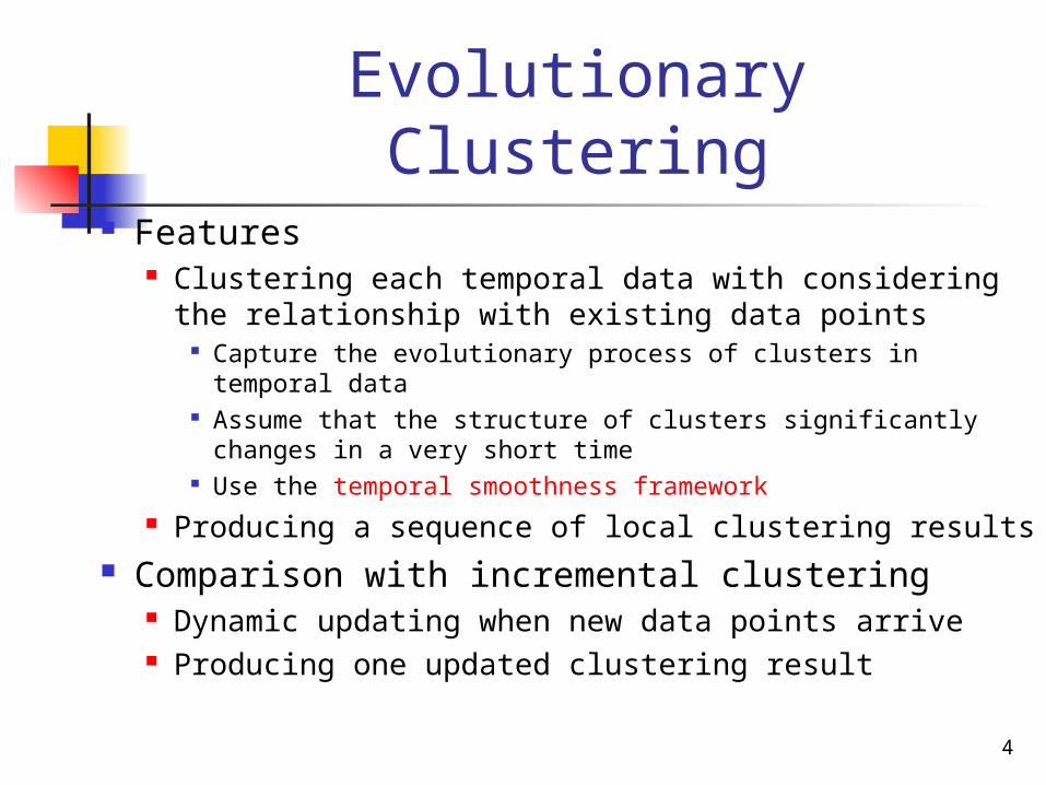
Evolutionary Clustering Features

Clustering each temporal data with considering the relationship with existing data points

Capture the evolutionary process of clusters in temporal data Assume that the structure of clusters significantly changes in a very

short time Use the temporal smoothness framework

Producing a sequence of local clustering results Comparison with incremental clustering

Dynamic updating when new data points arrive Producing one updated clustering result

4

Temporal Smoothness

Trying to smooth out each cluster over time By trading off between snapshot quality and history quality

Snapshot quality: how accurately the clustering result captures the structure of current network

History quality: how similar the current clustering result is with the previous clustering result

By using user-specific parameter α Cost function minimize it

High α : better snapshot quality Low α : better history quality

5

Motivation Previous evolutionary clustering methods

Assume only a fixed number of clusters over time Not allow arbitrary start/stop of community over time

However, the forming of new communities and dissolving of existing communities are quite natural and common phenomena in real dynamic networks Ex: research groups form or dissolve at some time in the co-

authorship dynamic network from the DBLP data

6

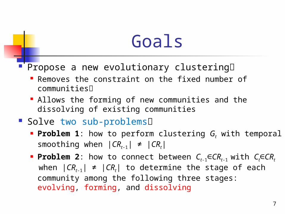
Goals Propose a new evolutionary clustering

Removes the constraint on the fixed number of communities Allows the forming of new communities and the dissolving of

existing communities Solve two sub-problems

Problem 1: how to perform clustering Gt with temporal smoothing when |CRt-1| ≠ |CRt|

Problem 2: how to connect between Ct-1∈CRt-1 with Ct∈CRt when |CRt-1| ≠ |CRt| to determine the stage of each community among the following three stages: evolving, forming, and dissolving

7

Definitions of symbols

8

Modeling of Community Nano-Community

Definition Neighborhood N(v) of a node v∈Vt = {x∈ Vt | ⟨v, x∈Et} {∪ v}

Nano-community NC(v, w) of two nodes v∈Vt -1 and w∈ Vt is defined by a sequence [N(v), N(w)] having a non-zero score for a similarity function Γ: N( ) ×⋅ N( ) →⋅ ℜ

Features A kind of particle capturing how dynamic networks evolve over time at

a nano level Can be represented by a link

9

Similarity Function ΓE()

Similarity function ΓE()

Example

10

otherwise ,0

exists , edgecommon a

or if ,1

))(),(( wv

wv

wNvNE

a

b

dc

a

b

dc

e

Gt-1 Gt

N(a)

N(a)NC(a,a)NC(a,b)

N(b)

NC(a,d)

N(d)Links

between a and Gt

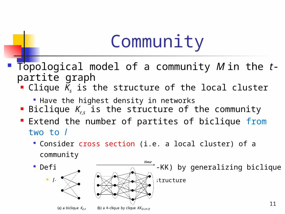
Community Topological model of a community M in the t-partite graph

Clique Ks is the structure of the local cluster Have the highest density in networks

Biclique Kr,s is the structure of the community Extend the number of partites of biclique from two to l

Consider cross section (i.e. a local cluster) of a community

Define l-clique-by-clique (l-KK) by generalizing biclique

l-KK is the densest community structure

11

Quasi l-KK In real applications, most of communities have the looser

structure, i.e., quasi l-KK Data inherent quasi l-KKs in a given dynamic network

Have relatively dense links and edges Provide guidance on how to find the communities

12t1 t2 t3 t4 t5

Clustering with temporal smoothing Previous methods

Adjust the clustering result CRt itself iteratively (⇒degrade performance)

Smooth Ct∈CRt by using the corresponding Ct-1∈CRt-1 (⇒require 1:1 mapping)

Four cases of the relationship between two nodes v and w at timestamps t-1 and t

Case 2: When α ↑ v, w in the same cluster at t When α ↓ v, w in the different cluster at t

13

Cost Embedding Technique The method proposed in this paper

No iterative adjusting CRt by pushing down the cost formula into the node distance dt (⇒no degrading performance)

Smoothing at the data level, which is independent of clustering results (⇒no requirement of 1:1 mapping)

where: do(v, w): original distance between v and w at time t without temporal

smoothing dt(v, w): smoothed distance between v and w at time t

SCN =│ do(v, w)- dt(v, w)│, TCN =│ dt-1(v, w)- dt(v, w)│

14

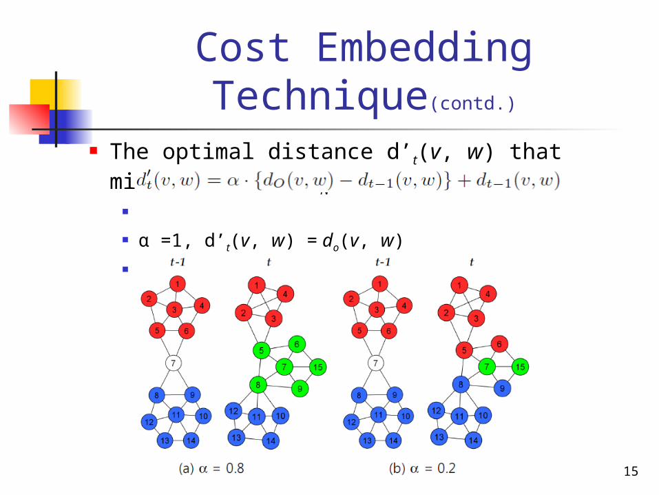
Cost Embedding Technique(contd.)

The optimal distance d’t(v, w) that minimize the costN

α =1, d’t(v, w) = do(v, w)

α =0, d’t(v, w) = dt-1(v, w)

15

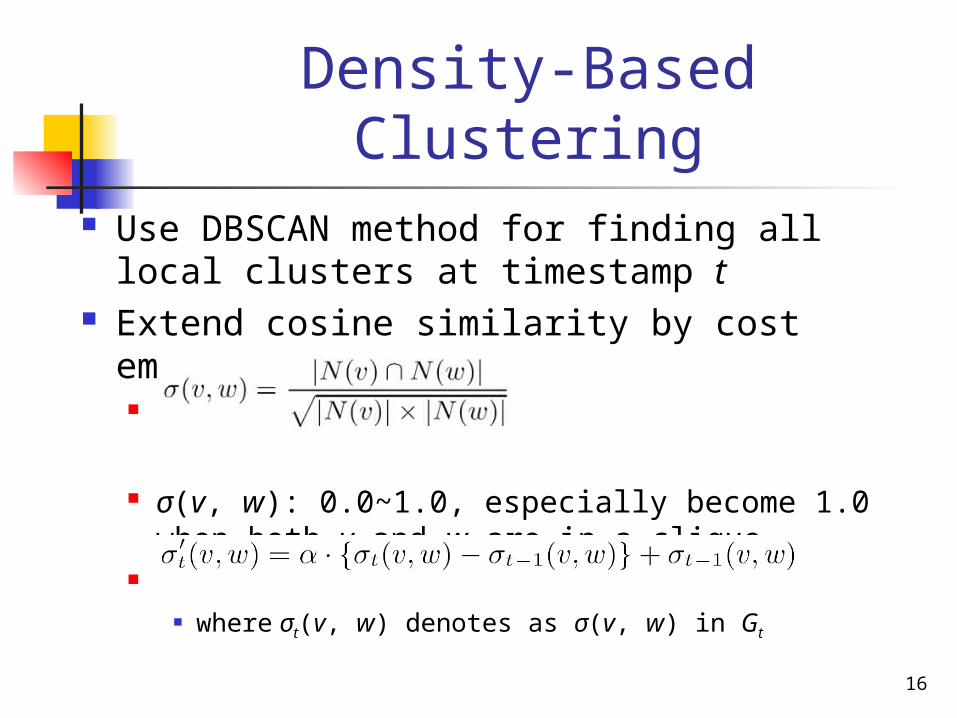
Density-Based Clustering Use DBSCAN method for finding all local clusters at

timestamp t Extend cosine similarity by cost embedding technique

σ(v, w): 0.0~1.0, especially become 1.0 when both v and w are in a clique

where σt(v, w) denotes as σ(v, w) in Gt

16

Clustering of Optimal Modularity DBSCAN requires two kinds of user-defined

parameters εt: specify the minimum similarity between nodes within a

cluster μt: specify the minimum size of cluster

Clustering result is sensitive to εt, but not much sensitive to μt

Determine εt automatically by using the novel concept of modularity

17

Clustering of Optimal Modularity(contd.)

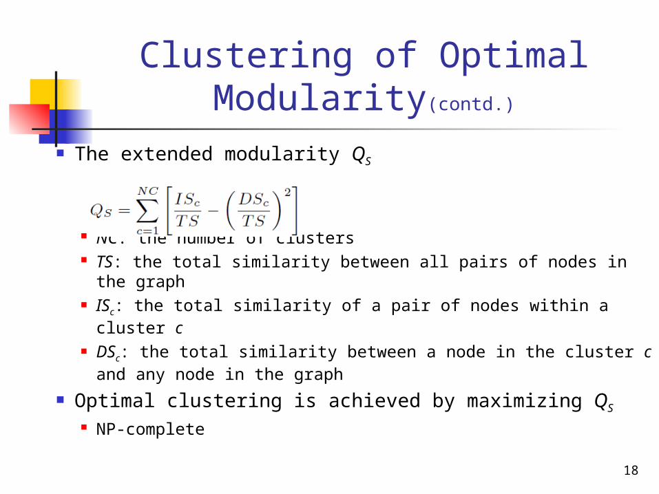
The extended modularity QS

NC: the number of clusters TS: the total similarity between all pairs of nodes in the graph ISc: the total similarity of a pair of nodes within a cluster c

DSc: the total similarity between a node in the cluster c and any node in the graph

Optimal clustering is achieved by maximizing QS

NP-complete18

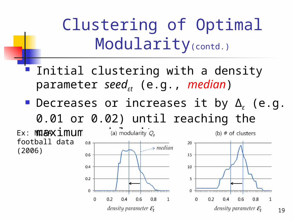
Clustering of Optimal Modularity(contd.)

Initial clustering with a density parameter seedεt (e.g., median)

Decreases or increases it by Δε (e.g. 0.01 or 0.02) until reaching the maximum modularity

19

Ex: NCAA football data (2006)

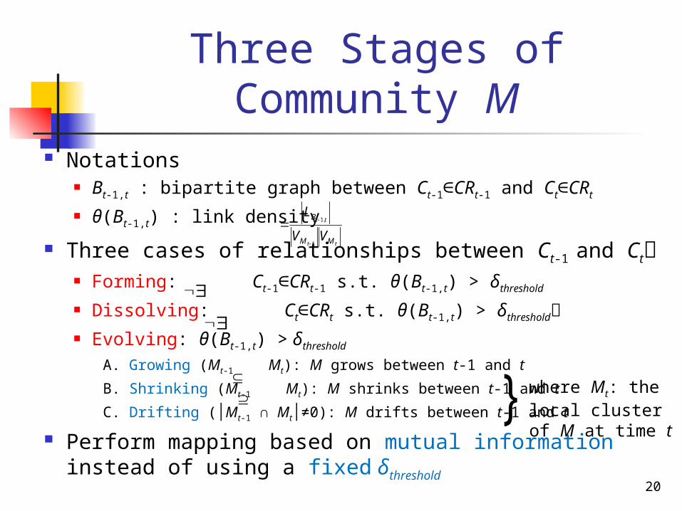
Three Stages of Community M Notations

Bt-1,t : bipartite graph between Ct-1∈CRt-1 and Ct∈CRt

θ(Bt-1,t) : link density

Three cases of relationships between Ct-1 and Ct Forming: Ct-1∈CRt-1 s.t. θ(Bt-1,t) > δthreshold

Dissolving: Ct∈CRt s.t. θ(Bt-1,t) > δthreshold

Evolving: θ(Bt-1,t) > δthreshold

A. Growing (Mt-1 Mt): M grows between t-1 and t

B. Shrinking (Mt-1 Mt): M shrinks between t-1 and t

C. Drifting (│Mt-1 ∩ Mt│≠0): M drifts between t-1 and t

Perform mapping based on mutual information instead of using a fixed δthreshold

20

tt

tt

MM

B

VV

L

1

,1

where Mt: the local cluster of M at time t}

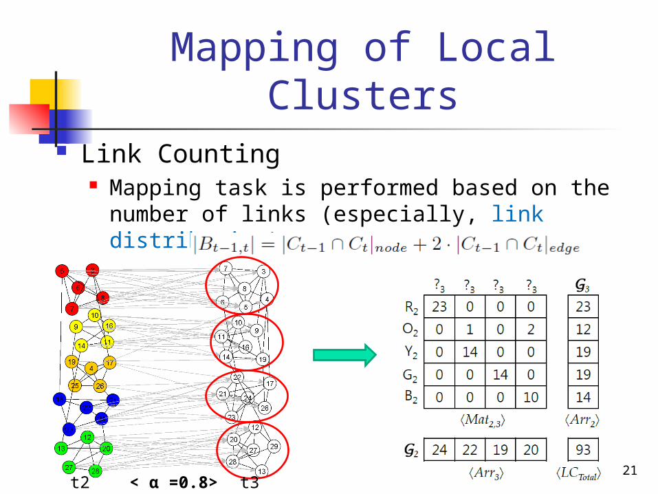
Mapping of Local Clusters Link Counting

Mapping task is performed based on the number of links (especially, link distribution)

Lemma:

21t2 t3< α =0.8>

Mutual Information Mutual information equation

Properties If the distribution of P(X) and P(Y) is purely random

MI(X; Y) becomes 0 If the distribution of P(X) and P(Y) is skewed

MI(X; Y) becomes high

22

Purifying Process If the relatively low probability value is set as zero

Purify the distribution more, MI(X; Y) increases Derivation of MI equation for link distribution

23unit MI

Purifying Process (contd.)

Mapping between Ct-1 and Ct indicates Making all cells of Matt-1,t[Ct-1][ ] and ⋅ Matt-1,t[ ][⋅ Ct] except

Matt-1,t[Ct-1] [Ct] zero and updating Arrt-1 ,Arrt, and LCTotal

Combinatorial optimization problem Choose at most min(|CRt-1|, |CRt|) pairs from |CRt-1|×|CRt|

pairs Propose an heuristic algorithm for maximizing MI

First choose ⟨Ct-1, Ct having the ⟩ highest unit MI

24

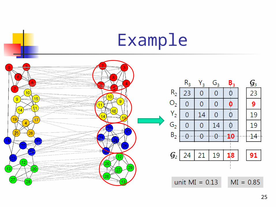
Example

25

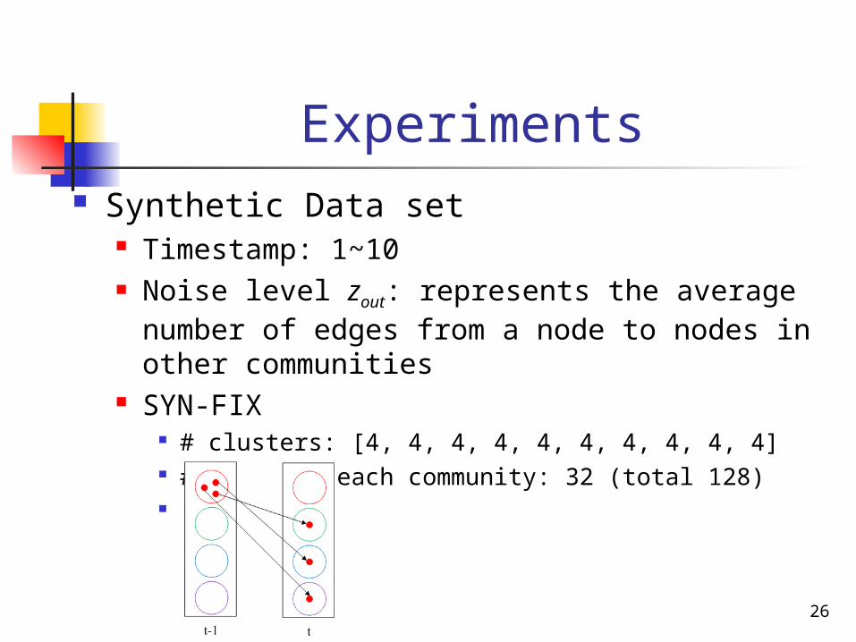
Experiments Synthetic Data set

Timestamp: 1~10 Noise level zout: represents the average number of edges from

a node to nodes in other communities SYN-FIX

# clusters: [4, 4, 4, 4, 4, 4, 4, 4, 4, 4] # nodes in each community: 32 (total 128)

26

Experiments (contd.)

SYN-VAR # clusters: [4, 5, 6, 7, 8, 8, 7, 6, 5, 4] # nodes / cluster: 32 ~ 64 (total 256) , lasting for 5 timestamps and its nodes return to

the original clusters

27

Experiments (contd.)

Real Data DBLP

co-authorship information 127,214 unique authors 10 years from 1999 to 2008

Measure Effectiveness: Normalized Mutual Information (called NMI)

between the ground truth and the clustering result Higher NMI indicates better accuracy

Efficiency: running time (sec.)28

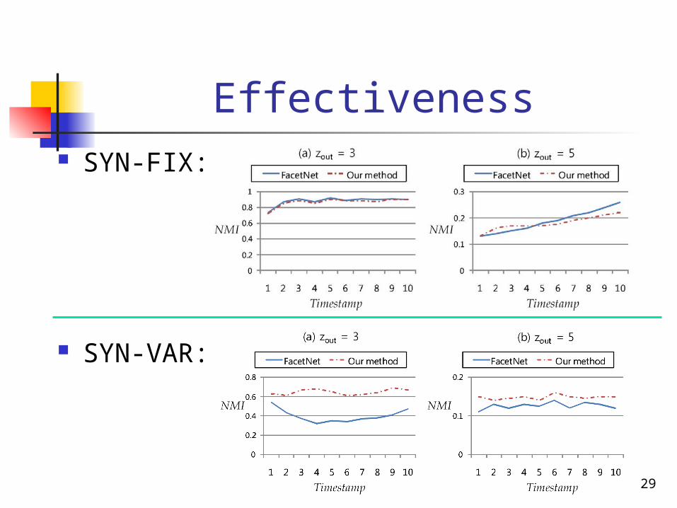
Effectiveness SYN-FIX:

SYN-VAR:

29

Efficiency Improve the time performance over 10 times

Due to avoiding a lot of iterations Suitable for large-scale dynamic network data

30

DBLP Data When α is high,

Communities become less temporal smooth The number of communities increases

A local cluster is not connected with other local cluster due to the low density between them

The average lifetime of community decreases Low α shows the opposite trend

31

Conclusions Propose particle-and-density based evolutionary clustering

method Nano-community (particle) & quasi l-KK (density)

Provide guidance on how to discover a variable number of communities of arbitrary forming and dissolving

Cost-embedding technique & density-based clustering using optimal modularity

Not require 1:1 mapping for temporal smoothing Achieve high clustering quality and time performance

Mapping method based on mutual information Make sequence of local clusters as close as possible to data inherent quasi

l-KKs

32