AFRL-IF-RS-TR-2005-151

Final Technical Report April 2005 A PARAMETRIC MODEL FOR LARGE SCALE AGENT SYSTEMS University of Illinois at Urbana-Champaign Sponsored by Defense Advanced Research Projects Agency DARPA Order No. K545

APPROVED FOR PUBLIC RELEASE; DISTRIBUTION UNLIMITED.

The views and conclusions contained in this document are those of the authors and should not be interpreted as necessarily representing the official policies, either expressed or implied, of the Defense Advanced Research Projects Agency or the U.S. Government.

AIR FORCE RESEARCH LABORATORY INFORMATION DIRECTORATE

ROME RESEARCH SITE ROME, NEW YORK

STINFO FINAL REPORT This report has been reviewed by the Air Force Research Laboratory, Information Directorate, Public Affairs Office (IFOIPA) and is releasable to the National Technical Information Service (NTIS). At NTIS it will be releasable to the general public, including foreign nations. AFRL-IF-RS-TR-2005-151 has been reviewed and is approved for publication APPROVED: /s/

JAMES M. NAGY Project Engineer

FOR THE DIRECTOR: /s/

JOSEPH CAMERA, Chief Information & Intelligence Exploitation Division Information Directorate

REPORT DOCUMENTATION PAGE Form Approved

OMB No. 074-0188 Public reporting burden for this collection of information is estimated to average 1 hour per response, including the time for reviewing instructions, searching existing data sources, gathering and maintaining the data needed, and completing and reviewing this collection of information. Send comments regarding this burden estimate or any other aspect of this collection of information, including suggestions for reducing this burden to Washington Headquarters Services, Directorate for Information Operations and Reports, 1215 Jefferson Davis Highway, Suite 1204, Arlington, VA 22202-4302, and to the Office of Management and Budget, Paperwork Reduction Project (0704-0188), Washington, DC 20503 1. AGENCY USE ONLY (Leave blank)

2. REPORT DATEAPRIL 2005

3. REPORT TYPE AND DATES COVERED Final Jun 00 – Jan 05

4. TITLE AND SUBTITLE A PARAMETRIC MODEL FOR LARGE SCALE AGENT SYSTEMS

6. AUTHOR(S) Gul Agha

5. FUNDING NUMBERS C - F30602-00-2-0586 PE - 62301E PR - TASK TA - 00 WU - 08

7. PERFORMING ORGANIZATION NAME(S) AND ADDRESS(ES) University of Illinois at Urbana-Champaign 109 Coble Hall 801 South Wright Street Champaign Illinois 61829-6200

8. PERFORMING ORGANIZATION REPORT NUMBER

N/A

9. SPONSORING / MONITORING AGENCY NAME(S) AND ADDRESS(ES) Defense Advanced Research Projects Agency AFRL/IFED 3701 North Fairfax Drive 525 Brooks Road Arlington Virginia 22203-1714 Rome New York 13441-4505

10. SPONSORING / MONITORING AGENCY REPORT NUMBER

AFRL-IF-RS-TR-2005-151

11. SUPPLEMENTARY NOTES AFRL Project Engineer: James M. Nagy/IFED/(315) 330-3173/ James.Nagy@rl.af.mil

12a. DISTRIBUTION / AVAILABILITY STATEMENT APPROVED FOR PUBLIC RELEASE; DISTRIBUTION UNLIMITED.

12b. DISTRIBUTION CODE

13. ABSTRACT (Maximum 200 Words)The goal of this project was to develop new techniques for the construction, description, and analysis of multi-agent systems. The characteristics of systems being addressed include a high degree of non-determinism (resulting form a large number of interactions) and unpredictability of the environment in which the agents operate. Specifically, we implemented tools for building robust and dependable large-scale multi-agent systems and studied methods for predicting and analyzing the behaviors of such systems. The project developed coordination methods for systems consisting of large numbers of agents.

15. NUMBER OF PAGES422

14. SUBJECT TERMS Autonomous Agent, MAS, Multi-Agent System, Large Scale Agent System, Coordination Model, Cooperation, Actor Framework, Formal Theory, Stochastic, Cellular Automa, Auctioning Scheme, Dynamic Environment, Distributed Task

16. PRICE CODE

17. SECURITY CLASSIFICATION OF REPORT

UNCLASSIFIED

18. SECURITY CLASSIFICATION OF THIS PAGE

UNCLASSIFIED

19. SECURITY CLASSIFICATION OF ABSTRACT

UNCLASSIFIED

20. LIMITATION OF ABSTRACT

ULNSN 7540-01-280-5500 Standard Form 298 (Rev. 2-89)

Prescribed by ANSI Std. Z39-18 298-102

Table of Contents

1. Objective………………………………………………………………………….1 2. Approach…………………………………………………………………………2 3. Accomplishments…………………………………………………………….......4 3.1 Formal Analysis of Agent Systems……………………………………...4 3.1.1 Reasoning about Agent Specifications using Probabilistic Rewrite Theory………………………………………………...…4 3.1.2 Monitoring and Verification of Deployed Agent Systems……..5 3.2 Multi-agent Modeling………………………………………………...….6 3.2.1 The Constraint Optimization Framework……………………...6 3.2.2 The Dynamic Distributed Task Assignment Framework……..7 3.2.3 Cellular Automata-based Modeling…………………………….7 3.3 Coordination Framework: the Dynamic Forward/Reverse Auction- ing Scheme………………………………………………………………..8 3.4 Large-Scale Multi-Agent Simulation: the Adaptive Actor …………...9 3.4.1 Adaptive Agent Distribution………………………….…………9 3.4.2 Application Agent-Oriented Middle Agent Services……….….9 3.4.3 Message Passing for Mobile Agents…………………………...10 3.4.4 AAA for UAV Simulation……………………………………...10 3.4.5 Experimental Results……………………………………….…..11 3.5 Hardware Realization: The August 2004 Demo……………………...14 4. Publications……………………………………………………………………..16 4.1 2005………………………………………………………………………16 4.2 2004………………………………………………………………………17 4.3 2003………………………………………………………………………20 4.4 2002………………………………………………………………………21 Appendix A: Scalable Agent Distribution Mechanisms for Large-Scale UAV Simulation……………………………………………………………….22 Appendix B: Efficient Agent Communication in Multi-Agent Systems…………….28 Appendix C: Online Efficient Predictive Safety Analysis of Multi-Threaded……...46 Appendix D: An Instrumentation Technique for Online Analysis of Multi-Thread Program………………………………………………………………….60 Appendix E: On Parallel vs. Sequential Threshold Cellular Automat…….………..71 Appendix F: Online Efficient Predictive Safety Analysis of Multithreaded Programs……………………………………………………………….…91 Appendix G: A Flexible Coordination Framework For Application Oriented Matchmaking and Brokering Services……………………………….106 Appendix H: A Perspective on the Future of Massively Parallel Computing: Fine Grain vs. Coarse-Grain Parallel Models……………………………..130 Appendix I: Concurrency vs. Sequential Interleavings in l-D Threshold Cellular Automata………………………………………………………………..145 Appendix J: An Instrumentation Techniques for Online Analysis of Multi- Threaded Programs……………………………………….……………153

i

Appendix K: Efficient Decentralized Monitoring of Safety in Distributed Systems…………………………………………………………….……161 Appendix L: On Efficient Communication and Service Agent Discovery in Multi- Agent Systems…………………………………………………………..171 Appendix M: On Specifying and Monitoring Epistemic Properties of Distributed Systems…………………………………………………………………178 Appendix N: Statistical and Monitoring Epistemic Properties of Distributed Systems…………………………………………………………………182 Appendix O: Maximal Clique Based Distributed Group Formations for Autonomous Agent…………………………………………………....195 Appendix P: ATSpace: A Middle Agent to Support Application Oriented Matchmaking & Brokering Services…………………………….…….203 Appendix Q: Learning Continuous Time Markov Chains from Sample Executions…………………………………………………….………..207 Appendix R: Towards Hierarchical Taxonomy of Autonomous Agents……….….217 Appendix S: Characterizing Configuration Spaces of Simple Threshold Cellular Automata……………………………………………………..223 Appendix T: On Challenges on Modelling and Designing Resource Bounded Autonomous Agents Acting in Complex Dynamic Environments…233 Appendix U: Some Modeling for Autonomous Agents Action Selection in Dynamic Partially Observable Environments…………………….….239 Appendix V: Task Assignment for a Physical Agent Team via a Dynamic Forward/Reverse Auction Mechanism………………………………245 Appendix W: Dynamic Agent Allocation for Large-Scale Multi-Agent Applications……………………………………………………………252 Appendix X: Maximal Clique Based Distributed Group Formation for Task Allocation in Large-Scale Multi-Agent Systems……………………..267 Appendix Y: Generating Optimal Monitors for Extended Regular Expressions…282 Appendix Z: Modeling A System of UAV’s On a Mission………………………….302 Appendix AA: Runtime Safety Analysis of Multi-threaded Programs……………309 Appendix AB: Simple Genetic Algorithms for Pattern Learning the Role of Crossovers………………………………………………………….….319 Appendix AC: An Actor-Based Simulation for Studying UAC Coordination….…323 Appendix AD: A Rewriting Based Model for Probabilistic Distributed Object Systems………………………………………………………………...332 Appendix AE: An Executable Specification of Asynchronous Pi-Calculus Semantics and May Testing in Maude 2.0…………………………..347 Appendix AF: Generating Optimal Linear Temporal Logic Monitors by Coinduction……………………………………………………….…..368 Appendix AG: An Executable Specification of Asynchronous Pi-Calculus Semantics in May Testing in Maude 2.0……………………….…...383 Appendix AH: Thin Middleware for Ubiquitous Computing……………….……..404

ii

List of Figures

Figure 1: Inter-roles Interaction in the Forward/Reverse Auction Protocol………………8 Figure 2: Three-Layered Architecture for UAV Simulations……………………………11 Figure 3: ASC of UAVs for Performing a Given Mission………………………………12 Figure 4: Runtimes for Static and Dynamic Agent Distribution………………………...13 Figure 5: Experimental Environment…………………………………………………….14

iii

1 OBJECTIVE The goal of this project was to develop new techniques for the construction, description, and analysis of multi-agent systems. The characteristics of systems being addressed include a high degree of non-determinism (resulting from a large number of interactions) and unpredictability of the environment in which the agents operate. Specifically, we implemented tools for building robust and dependable large-scale multi-agent systems and studied methods for predicting and analyzing the behaviors of such systems. The project developed coordination methods for systems consisting of large numbers of agents.

1

2 APPROACH In order to effectively model large-scale systems, it is necessary to focus on properties of interest at a macroscopic level. Therefore, we used a divide and conquer approach in addressing the construction and analysis of large-scale agent systems and we modeled agent systems at two levels of abstractions: the system level and the application level.

Our goal at the system or implementation level was to ease the construction and analysis of dependable large-scale agent systems. At this level, we modeled agents as autonomous entities that interact via message passing schemes. Therefore, the actor framework provided a good starting point because it does not make any assumptions or stipulations about the logic of the application for which the actors are developed. The actor framework also has a rich formal theory that we extended and used to study high level specifications of agent systems. The formalisms we developed abstract irrelevant details and focus directly on the desired macroscopic properties. Furthermore, methods for modular and compositional specifications were considered so that simple specifications of specific properties or components can be composed to derive more complex specifications of larger systems.

Moreover, large-scale agent systems are inherently stochastic. The asynchrony and autonomy of widely distributed agents inevitably leads to non-determinism. This may be the case irrespective of the nature individual agent behaviors which might be deterministic or stochastic. The methods we developed accounted for this uncertainty by allowing stochastic descriptions of agent systems and providing techniques to reason about the likelihoods of possible evolutions of the systems.

In spite of the advantages of formal analysis, it has serious limitations when applied to large-scale agent systems. Typically, in order to keep the analysis tractable, one chooses only a few relevant abstractions to describe and reason about the system. While this is effective for certain purposes, formal analysis is not feasible for problems involving too many parameters. To address this problem, we developed the Adaptive Actor Architecture (AAA) which utilized various optimizing techniques to simulate large-scale agent system and derive empirical estimations of the desired properties.

We viewed our work at the system level as an enabling technique that facilitates the construction and testing of various multi-agent coordination models. These models focus only on the application logic at high levels of abstractions and are not concerned with the architecture used to implement the agents. Moreover, the work at the application level stimulated and motivated our work at the system level to cope with the scalability requirement of the application needs. Therefore, we used an evolutionary approach in which each level bootstrapped progress at the other one.

Our goal at the application or coordination level was to develop models and techniques that facilitate multi-agent teamwork or how to allow a group of agents to cooperate in order to

2

accomplish a high level team goal. To achieve this, we developed theoretical models that help us to understand the difficulty of multi-agent teamwork and provide a framework to parametrically analyze the tension between different aspects of the teamwork coordination problems. Specifically, we developed the distributed constraint optimization framework and we also used cellular automata to mathematically model multi-agent systems. We studied the role of agent autonomy in teamwork and developed natural epistemological and hierarchical taxonomy of different types of autonomous agents, strictly based on an agent's critical capabilities as seen by an outside observer.

While the above models were geared toward fostering our understanding of the teamwork problem, they were not suitable to serve as an executable model that enables each agent to decide about what action to do. Nevertheless, these efforts helped us to arrive at the proper level of abstraction to attack the teamwork problem. We represented the multi-agent teamwork problems as a distributed task assignment problem in which a group of agents is required to accomplish a set of tasks while maximizing a certain performance measures. We developed the dynamic forward/reverse auctioning scheme as a generic method for solving the distributed task assignment problem in dynamic environments.

To measure our progress at both the system and application levels, we used the TASK shared domain, viz, Unmanned Aerial Vehicle (UAV). Using our AAA, we developed large simulations agents modeling up to 10,000 UAVs in a surveillance task, contrasting different coordination approaches for this task. We also modeled the problem of a team of UAVs in a search and rescue mission using our dynamic distributed task assignment framework and our dynamic auctioning scheme to derive agents' behavior in this domain. We evaluated this approach using physical agents, i.e., robots. The robot-based simulation consisted of up to 20 robots forming dynamic teams to carry out the surveillance task.

3

3 ACCOMPLISHMENTS 3.1 Formal Analysis of Agent Systems

In order to facilitate the analysis of the behavior of agent systems, it was necessary to develop techniques for specifying and reasoning about such systems. We have shown that these techniques can make use of three fundamental properties of agent systems:

• Asynchrony: Autonomous agents operate and communicate asynchronously. • Modularity: Agent systems can be decomposed into concurrent components, each

consisting of an ensemble of agents. • Locality and Non-interference: Messages between agents are the only means of

information flow, e.g., there are no shared variables.

We leveraged these properties in achieving significant progress in two main areas: rewrite theory and distributed monitoring of multi-agent systems.

3.1.1 Reasoning about Agent Specifications Using Probabilistic Rewrite Theory

We decided to extend the rewrite framework and use it for specification and reasoning about large-scale agent systems. The rewrite theory is an appealing formalism because of its support for abstraction by providing the ability to group several agent states into a single state, and several low level transitions into a big step transition. For example, a rule could abstractly state in a single step the transition of a group of agents from before a leader election procedure to after. Specifically, the final state of the group is specified without furnishing the details of how the transition is implemented. Therefore it results in a compact specification.

Nondeterminism exhibits itself in the system when two or more rules may be simultaneously applicable to a certain state. When such rules do not conflict they are allowed to proceed either concurrently or in an interleaving fashion. On the other hand, if the rules conflict, the system decides which rule to apply according to customizable probabilistic tactics. To enable such probabilistic tactics, we extended this rich formalism with probabilistic transitions which results in the Probabilistic Rewrite Theory formalism. We made significant progress in providing a precise formulation and semantic for this formalism.

We demonstrated how to use the Probabilistic Rewrite Theory to express systems with nondeterminism and probabilities, thus providing a way to reason about distributed systems, randomized algorithms, as well as systems where we have probabilistic models of communication delays, failures, etc. Moreover, we showed that Continuous Time Markov

4

Chains and Generalized Semi-Markov Processes can be naturally expressed in our rewriting model. We implemented a simulator for finitary probabilistic rewrite theories called PMaude. PMaude provides a tool to formally study agent systems, for example, to do performance modeling and studies of agent systems involving continuous variables.

3.1.2 Monitoring and Verification of Deployed Agent Systems

We used the actor properties (asynchrony, modularity, and locality) to develop a rich theory of agents. In particular, significant improvement can be made with respect to the efficiency of verification algorithms. We were able to show that instead of testing configurations under all possible execution environments -- an expensive and generally infeasible process because of the nondeterminism in agent systems -- it is possible to use an exponentially smaller set of traces which represents a canonical set of execution orders in such systems.

We also developed techniques for distributed monitoring of multi-agent systems. These techniques allow automatic generation of local monitoring code from a specification of a distributed property. The code is weaved with execution code to enable seamless monitoring of the specification. Finally, we developed methods for statistical black-box testing of probabilistic properties in a system

Finally, we developed techniques for the scalable statistical analysis of multi-agent systems. Specifically, we developed a new statistical approach for analyzing stochastic agent systems against specifications given in a sublogic of continuous stochastic logic (CSL). Unlike past numerical and statistical analysis methods, we assume that the system under investigation is an unknown, deployed black-box that can be passively observed to obtain sample traces, but cannot be controlled. Given a set of executions (obtained by Monte Carlo simulation) and a property, our techniques check, based on statistical hypothesis testing, whether the sample provides evidence to conclude the satisfaction or violation of a property, and computes a quantitative measure (p-value of the tests) of confidence in its answer; if the sample does not provide statistical evidence to conclude the satisfaction or violation of the property, the algorithm may respond with a “don't know” answer.

5

3.2 Multi-agent Modeling

We have made significant progress in modeling multi-agent systems at the application level. Some of these models strive to provide a theoretical foundation to understand the difficulty of multi-agent coordination. They make use of rigorous mathematical optimization and models based on cellular-automata. Motivated by this analysis we also defined the dynamic distributed task assignment problem that enables us to use economic models to provide near optimal solutions under resource constraints.

3.2.1 The Constraint Optimization Framework

The goal of the constraint optimization framework is to mathematically provide a parametric model of a system of agents working as a team to accomplish a set of tasks while satisfying a heterogeneous set of physical and communication constraints. We used this framework to model a team of UAVs in a surveillance task. Specifically, we applied the framework to UAVs, where we model each UAV as an autonomous agent. Each agent has an individual utility and the goal of the system is to maximize a joint utility function. The application requires each UAV to plan its path in cooperation with other UAVs in order to accomplish an aerial survey of dynamically evolving targets. In this framework, we assumed the existence of a common clock and the ability of agents to communicate with each other in a given communication range by means of multi-cast messages. We also assumed that a certain number of geographical locations were of interest, and their value was dynamically changing over time.

Guided by the above formulation, and using our simulation environment (see Section 4), we simulated a number of agent strategies to understand the tension between variables in our parametric model. The simulation modeled UAV's intrinsic kinematics such as velocity and acceleration, constraints on each UAV's trajectory (e.g., collision avoidance), and constraints on resources such as fuel, available air corridors, and bounded communication radii. Each UAV's utility function was dependent on its position and the expected value of a target by the time the UAV would arrive there. In our model the value of the target declines with time. These set of simulations suggested two tentative conclusions:

There is an optimal number of UAVs for a given problem which can be established through our simulation engine. Beyond this number, more UAVs have a marginal negative impact on pay-offs. As we scale up, locality becomes more important than the utility of a target.

Moreover, we devised special algorithms to efficiently solve a certain instance of the constraint optimization problem were the goal is to form coalition among agents under the constraint of achieving maximal cliques in the underlying communication topology. This problem was directly motivated by multi-agent environments and applications where both node and link failures are to be expected, and where group and coalition robustness with respect to such failures is a highly desirable quality. These cliques, however, are restricted

6

to be of smaller than a given maximum ceiling size. This restriction allows computational tractability despite the fact that the general MAX-CLIQUE problem is NP-complete.

3.2.2 The Dynamic Distributed Task Assignment Framework

Using the constraint optimization framework we arrived at the proper level of abstraction to attack the teamwork problem. We realized, among other researchers albeit using a different formulation, that many multi-agent teamwork problems can be modeled as a Dynamic Distrusted Task Assignment (DDTA) problem. In the DDTA problem, a group of agents is required to accomplish a set of tasks while maximizing a certain performance measure. We identified that an effective solution to the DDTA problem needs to address two closely related questions:

1. How to find a near-optimal assignment from agents to tasks under resource constraints?

2. How to efficiently maintain the optimality of the assignment over time?

Guided by this formulation, we developed our solution to the DDTA problem, the Dynamic Forward/Reverse Auctioning scheme, described in Section 3. We applied this scheme to a UAV search and rescue scenario with promising results (see Section 5).

3.2.3 Cellular Automata-based Modeling

We made progress in developing a "starting point" mathematical model for agent systems using the classical cellular automata (CA). We intensely studied some extensions and modifications of the classical CA, so that the resulting graph or network automata are more faithful abstractions of a broad variety of large-scale multi-agent systems. We also developed natural epistemological and hierarchical taxonomy of different types of autonomous agents, strictly based on an agent's critical capabilities as seen by an outside observer.

7

3.3 Coordination Framework: The Dynamic Forward/ Reverse Auctioning Scheme

The goal of the dynamic forward/reverse auction mechanism is to solve the dynamic distributed task assignment problem as posed in Section 2.2. A solution to the DDTA problem should ensure that task-agent assignment is always optimal with respect to the performance measure. Our approach can be characterized as a divide and conquer method that separately deals with combinatorial complexity and dynamicity – the two aspects of the DDTA problem. We addressed the first issue by extending an existing forward/reverse auction algorithm which was designed for bipartite maximal matching to find an initial near-optimal assignment. The extension makes it suitable for the distributed, asynchronous, multi-requirement aspects of the DDTA problem. However, the dynamicity of the environment compromises the optimality of the initial solution obtained via this modified algorithm. We address the dynamicity problem by using swapping to locally move agents between tasks. By linking these local swaps, the current assignment is morphed into one which is closer to what would have been obtained if we had re-executed the computationally more expensive auction algorithm.

We applied this dynamic auctioning scheme in the context of UAVs (Unmanned Aerial Vehicles) search and rescue mission and developed experiments using physical agents to show the feasibility of the proposed approach in the TASK August demo which featured twenty robots (targets and pursuers). Besides the experimental results, we conducted a theoretical analysis about the performance of swapping.

Bidding

Auction Start

Collecting Bids

Round End

Reverse Step

Auction End

Announce

Task Auctioneer

No Target

New Target

Servicing Target

Won Auction

Bidding

No Target

New Target

Servicing Target

Won Auction

New

Target

Announce Announce

Not Enough Bids

Enough Bids

Bidder Agent Bidder Agent

Figure 1: Inter-roles Interaction in the Forward/Reverse Auction Protocol

8

3.4 Large-scale Multi-agent Simulation: The Adaptive Actor Architecture

The Adaptive Actor Architecture (AAA) was one of the major accomplishments of this TASK project. The AAA is designed to support the construction of large-scale multi-agent applications by exploiting distributed computing techniques to efficiently distribute agents across a distributed network of computers. Distributing agents across nodes introduces inter-node communication that might eliminate any improvement in the runtime of large-scale multi-agent applications. The AAA uses several optimizing techniques to address three fundamental problems related to agent communication between nodes : agent distribution, service agent discovery and message passing for mobile agents. We will first discuss how these problems have been addressed in the AAA and then describe how the AAA was used in the UAV domain.

3.4.1 Adaptive Agent Distribution

Unless an agent requires some specific devices or services belonging to a certain computer node, the location of an agent does not affect the result of computation. However, the performance of agent applications may vary considerably according to the distribution pattern of agents, because agent distribution changes the inter-node communication pattern of agents, and the amount of inter-node communication considerably affects the overall performance. Therefore, if we could co-locate agents that intensively communicate with each other, the communication cost among agents could be minimized. Moreover, since the communication pattern of agents is continuously changing, agent distribution should be adaptive and dynamic .

If agents are dynamically distributed according to only their communication localities, some computer nodes could be overloaded with too many agents. Therefore, we distributed agents according to both their communication localities and the workload of computer nodes. The novel features of our approach are that this mechanism is based on the communication locality of agent groups as well as individual agents, and that the negotiation between computer nodes for agent migration occurs at the agent group level, but not at the individual agent level .

3.4.2 Application Agent-oriented Middle Agent Services

In open multi-agent systems where agents can enter and leave at any time, middle agent services such as brokering and matchmaking are very effective at finding service agents. Since brokering services can remove one message that may be very large , they may be more efficient than matchmaking services. However, because of the difficulty in expressing all search algorithms to a middle agent, in some cases we must use a matchmaking service

9

instead of brokering service. Previous solutions modify the search mechanism of the middle agent. But any change to the search mechanism in a middle agent affects other agents .

To handle the different interests of agents, we developed and implemented an active interaction model for middle agent services. In these services , the middle agent manages data, and search algorithms are given by application agents. With this separation of search algorithms from data, the middle agent can support the different interests of application agents at the same time without affecting other agents. Although application agents are located on different computer nodes, because their search algorithms are executed on the same computer node where data exist, the search algorithm can be performed efficiently, and the delivery overhead of search algorithms can be compensated with the performance benefit .

3.4.3 Message Passing for Mobile Agents

Message passing is the most fundamental service in multi-agent frameworks. Regardless of the locations of receiver agents, agent frameworks should provide reliable message passing. With dynamic agent distribution, agents may often change their locations . Sending a message to a mobile agent that has moved from its original computer node may require more than one message hop. If the sending node can directly deliver the message to the mobile agent, it will reduce communication time .

For this purpose, we developed a location-based message passing mechanism and a delayed message passing mechanism. The location-based message passing mechanism uses location information in the name of a receiver agent, and the name of an agent is updated by its current computer node whenever the agent changes its location. The delayed message passing mechanism allows a computer node to hold messages for a moving agent until the agent finishes its migration .

3.4.4 AAA for UAV Simulation

We used the AAA to build ActorSim with which we used to conduct several simulation runs to compare different coordination strategies for a UAV surveillance task. This simulation package provides simulation time management, environment-based agent interaction, kinematics of UAVs and targets, etc. We used this simulator to study the effectiveness of applying a number of multi-agent coordination mechanisms to the problem of cooperative surveillance in scenarios of up to 10,000 agents (5,000 UAVs and 5,000 targets). Moreover, we have designed a graphical simulation viewer for ActorSim in OpenGL. Good visualization is important not only for the spectators, but also for the designers of the higher-level system capabilities, such as, the agent capabilities of effective collaborative coordination and collision avoidance.

10

We have transferred a preliminary version of the ActorSim simulator and UAV simulation package to the Information Director of Air Force Research Laboratory (AFRL/IF) in Rome, NY. Rome Labs plans to customize the simulation toolkit for use by research teams at AFRL/IF.

Adaptive Actor Architecture - Adaptive Agent Distribution - Application Agent-oriented Middle Agent Services - Message Passing for Mobile Agents

Simulation Control Manager

Environment Simulator

Task-oriented Agents:

Simulation-oriented Agents:

UAVUAVUAVUAV

TargetTargetTargetTarget

ABS: Air Base System

GCS: Ground Control System

ActorSim

UAV Simulation Viewer - OpenGL based graphic viewer

Figure 2: Three-Layered Architecture for UAV Simulations

3.4.5 Experimental Results

To investigate how a cooperation strategy influences the performance of a joint mission, we use Average Service Cost (ASC) as our metric. ASC is interpreted as additional navigation time to serve given targets, and is defined as follows:

n

MNTNTASC

n

ii∑ −

=)(

11

where n is the number of UAVs, NTi means navigation time of UAV i, MNT (Minimum Navigation Time) means average navigation time of all UAVs required for a mission when there are no targets.

Figure 3 depicts ASC for a team-based coordination strategy and a self-interest strategy. When the number of UAVs is increased, ASC is decreased in every case. This result explains that communication of UAVs is useful to handle targets, even though UAVs in the self-interest UAV strategy consumes quickly the value of a target when they handle the target together.

0

2

4

6

8

10

12

14

16

1000 2000 3000 4000 5000Number of UAVs

(Number of Targets: 5000)

AS

C (M

inut

es)

Self-Interest

Team-basedCoordintion

Figure 3: ASC of UAVs for Performing a Given Mission

To evaluate the potential benefit of adaptive agent distribution of AAA, we conducted the same simulations with two different agent distribution strategies: dynamic agent distribution and static agent distribution. Figure 4 depicts the difference of runtimes of simulations in two cases. Even though the dynamic agent distribution in our simulations includes the overhead for monitoring and decision making, the overall performance of dynamic agent distribution overwhelms that of static agent distribution. As the number of agents is increased, the ratio also generally increases. With 10,000 agents, the simulation using the dynamic agent allocation is more than five times faster than the simulation with a static agent allocation.

12

0

10

20

30

40

50

60

2000 4000 6000 8000 10000

Number of Actors (UAVs + Targets)

Run

time

(Hou

rs)

StaticAgentDistributionDynamicAgentDistribution

Figure 4: Runtimes for Static and Dynamic Agent Distribution

13

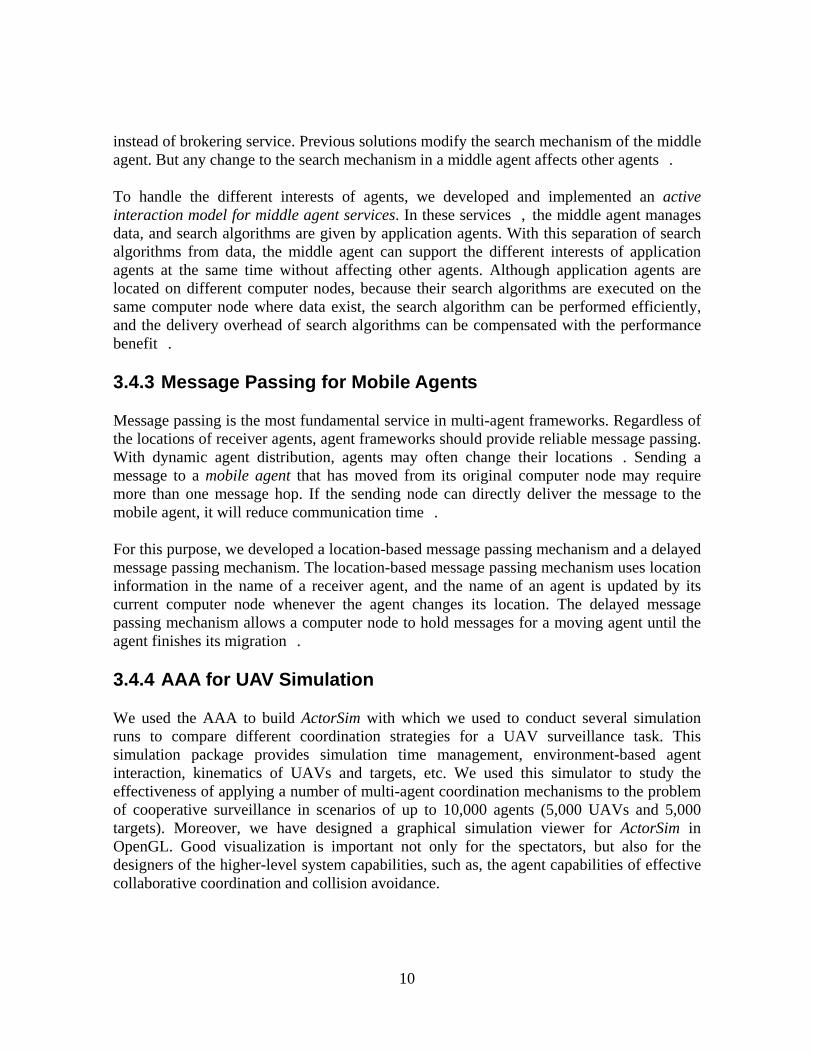
3.5 Hardware Realization: The August 2004 Demo

The goal of our August hardware demo was to demonstrate our techniques in a realistic environment. For this purpose, we created a search and rescue mission. In this domain, a collection of UAVs roam a rectangle mission area looking for targets (downed pilots, injured civilians, etc.). These targets move according to a pre-determined path not known to the UAVs. Each target has a step utility function and requires a minimum number of UAVs to be serviced. This step utility function means that before the target gets its required number of UAVs, none of its utility can be consumed by the team. Once a requisite number of UAVs arrive near the target, it is deemed to have been serviced. UAVs monitor targets and coordinate the groups that service them subject to maximizing the total team benefit. We have modeled the above scenario using the DDTA formulation as mentioned in Section 2.2 and applied our dynamic forward/reverse auction mechanism to derive agent behaviors in this domain.

Figure 5: Experimental Environment

We modeled UAVs and targets as robot cars. Each car was controlled by an iPAQ PDA running Microsoft Pocket PC and receives localization information from a leader vision server collaborating data from four vision servers, each of which is connected to an overhead video camera. A vision server takes images from a camera, searches for unique color plates mounted on each robot car, and calculates the corresponding robot’s identification and heading. A leader vision server takes localization information from each vision server, and sends filtered and regulated localization information to the iPAQs. The iPAQs use an internal WiFi interface for inter-agent communication. Different cars are used to represent UAVs and targets. It is quite clear that this hardware setting makes discovering logical errors in the software implementation and tracing the agents’ behavior very hard. To deal with these issues, we developed a hardware/software shared agent code

14

architecture that allows us to simulate this hardware setting in software while at the same time guaranteeing interoperability when porting this code to the hardware setting. The main design philosophy of the system was to ease parallel development and testing of the code. The agent’s (UAV/Target) implementation is isolated from the architecture on which the system is running. The system was developed to run in one of two modes: a simulated mode or a real node. This architecture helped us accelerate the development cycle when preparing for the hardware final demo.

Another technical issue we faced during this hardware demo, which was not apparent in software simulations, was collision avoidance. While collisions can be abstracted away in a large-scale software simulation of a multi-agent system, the issue is critical in the context of real vehicles. With up to twenty robots in our hardware demo, operating in a relatively small area (8 m × 6 m), collision avoidance poses significant challenges. To address this problem, we developed online path planning and re-planning heuristics for collision avoidance as well as group coordination behavior when pursuing the assigned target. All of these techniques were demonstrated successfully during a demonstration for DARPA in August 2004.

15

4 PUBLICATIONS 4.1 2005 Myeong-Wuk Jang and Gul Agha, "Scalable Agent Distribution Mechanisms for Large-Scale UAV Simulations," The International Conference of Integration of Knowledge Intensive Multi-Agent Systems KIMAS '05, Scalable Agents Session, Waltham, Massachusetts, April 18-21, 2005. Myeong-Wuk Jang, Amr Ahmed and Gul Agha, "Efficient Communication in Multi-Agent Systems," LNCS Special Issue on Software Engineering for Large Scale Multi-Agent Systems, to be published 2005. Koushik Sen, Grigore Rosu and Gul Agha, “Online Efficient Predictive Safety Analysis of Multithreaded Programs”, International Journal on Software Technology and Tools Transfer STTT, to appear 2005. Grigore Rosu and Koushik Sen, “An Instrumentation Technique for Online Analysis of Multithreaded Programs”, Special Issue of Concurrency and Computation: Practice and Experience (CC:PE), to appear 2005. Predrag Tosic and Gul Agha, "On Parallel vs. Sequential Threshold Cellular Automata," Technical Report, Department of Computer Science, University of Illinois at Urbana-Champaign, to appear 2005.

16

4.2 2004 Koushik Sen, Grigore Rosu and Gul Agha, “Online Efficient Predictive Safety Analysis of Multithreaded Programs,” In Proceedings of 10th International Conference on Tools and Algorithms for the Construction and Analysis of Systems TACAS ’04, Springer-Verlag Lecture Notes in Computer Science, volume 2988, Barcelona, Spain, March 29-April 2, 2004, pages 123-138. Myeong-Wuk Jang, Amr Ahmed and Gul Agha, "A Flexible Coordination Framework for Application-Oriented Matchmaking and Brokering Services," Technical Report UIUCDCS-R-2004-2430, Department of Computer Science, University of Illinois at Urbana-Champaign, April 2004. Predrag Tosic, "A Perspective on the Future of Massively Parallel Computing: Fine Grain vs. Coarse-Grain Parallel Models," Proceedings of the First ACM Conference on Computing Frontiers (CF '04), Ischia, Italy, April 14-16, 2004, pages 488-502. Predrag Tosic and Gul Agha, "Concurrency vs. Sequential Interleavings in 1-D Threshold Cellular Automata," Proceedings of The 18th International Parallel and Distributed Processing Symposium IPDPS '04, Advances in Parallel and Distributed Computing Models Workshop, Santa Fe, New Mexico, USA, April 26-30, 2004, page 179b. Grigore Rosu and Koushik Sen, “An Instrumentation Technique for Online Analysis of Multithreaded Programs,” Workshop on Parallel and Distributed Systems: Testing and Debugging PADTAD ’04, Santa Fe, New Mexico, USA, April 30, 2004, page 268. Koushik Sen, Abhay Vardhan, Gul Agha and Grigore Rosu, “Efficient Decentralized Monitoring of Safety in Distributed Systems,” In Proceedings of 26th International Conference on Software Engineering ICSE ’04, Edinburgh, Scotland, United Kingdom, May 23-28, 2004, pages 418-427. Myeong-Wuk Jang and Gul Agha, "On Efficient Communication and Service Agent Discovery in Multi-agent Systems," Third International Workshop on Software Engineering for Large-Scale Multi-Agent Systems (SELMAS '04), Edinburgh, Scotland, May 24-25, 2004, pages 27-33. Koushik Sen, Abhay Vardhan, Gul Agha and Grigore Rosu, “On Specifying and Monitoring Epistemic Properties of Distributed Systems,” Second International Workshop on Dynamic Analysis, WODA ’04, pages 32-35, Edinburgh, Scotland, United Kingdom, May 25, 2004, pages 32-35.

17

Koushik Sen, Mahesh Viswanathan and Gul Agha, “Statistical Model Checking of Black-Box Probabilistic Systems,” Proceedings from the 16th International Conference on Computer Aided Verification CAV ’04, Springer-Verlag, Lecture Notes in Computer Science, volume 3114, Boston, MA, USA, July 13-17, 2004, pages 202-215. Predrag Tosic and Gul Agha, "Maximal Clique Based Distributed Group Formation for Autonomous Agent Coalitions," Third International Joint Conference on Agents & Multi Agent Systems AAMAS '04, Coalitions and Teams Workshop, New York, New York, USA, July 19-23, 2004. Myeong-Wuk Jang, Amr Ahmed and Gul Agha, "ATSpace: A Middle Agent to Support Application-Oriented Matchmaking and Brokering Services," Proceedings of IEEE/WIC/ACM Intelligent Agent Technology 2004 (IAT ’04), Beijing, China, September 20-24, 2004, pages 393-396. Koushik Sen, Mahesh Viswanathan and Gul Agha, “Learning Continuous Time Markov Chains from Sample Executions,” First International Conference on Quantitative Evaluation of Systems QEST ’04, Enschede, The Netherlands, September 27-30, 2004, pages 146-155. Predrag Tosic and Gul Agha, "Towards a Hierarchical Taxonomy of Autonomous Agents," Proceedings from the. IEEE International Conference on Systems, Man and Cybernetics SMC '04, The Hague, The Netherlands, October 10-13, 2004. Predrag Tosic and Gul Agha, "Characterizing Configuration Spaces of Simple Threshold Cellular Automata," Sixth International Conference on Cellular Automata for Research and Industry, Amsterdam, The Netherlands, October 25-27, 2004, Springer-Verlag, Lecture Notes in Computer Science, volume 3305, 2004, pages 861-870. Predrag Tosic and Gul Agha, "On Challenges in Modeling and Designing Resource-Bounded Autonomous Agents Acting in Complex Dynamic Environments," Proceedings of the IASTED International Conference on Knowledge Sharing and Collaborative Engineering KSCE '04, St. Thomas, US Virgin Islands, November 22-24, 2004. Predrag Tosic and Gul Agha, "Some Models for Autonomous Agents' Action Selection in Dynamic Partially Observable Environments," Proceedings from the IASTED International Conference on Knowledge Sharing and Collaborative Engineering KSCE '04, St. Thomas, US Virgin Islands, November 22-24, 2004. Amr Ahmed, Abhilash Patel, Tom Brown, MyungJoo Ham, Myeong-Wuk Jang and Gul Agha, "Task Assignment for a Physical Agent Team via a Dynamic Forward/Reverse Auction Mechanism," Technical Report UIUCDCS-R-2004-2507, Department of Computer Science, University of Illinois at Urbana-Champaign, December 2004.

18

Myeong-Wuk Jang and Gul Agha, "Dynamic Agent Allocation for Large-Scale Multi-Agent Applications," International Workshop on Massively Multi-Agent Systems, Kyoto, Japan, December 10-11, 2004, pages 19-33. Predrag Tosic and Gul Agha, "Maximal Clique Based Distributed Group Formation for Task Allocation in Large-Scale Multi-Agent Systems," Proceedings from the Workshop on Massively Multi-Agent Systems, Kyoto, Japan, December 10-11, 2004.

19

4.3 2003 Koushik Sen and Grigore Rosu, "Generating Optimal Monitors for Extended Regular Expressions," Proceedings of 3rd Workshop on Runtime Verification RV ’03, Elsevier Science Electronic Notes in Theoretical Computer Science, volume 89, issue 2, Boulder, Colorado, USA, July 13, 2003. Predrag Tosic, Myeong-Wuk Jang, Smitha Reddy, Joshua Chia, Liping Chen and Gul Agha, "Modeling a System of UAVs on a Mission," Proceedings of the. 7th World Multiconference on Systemics, Cybernetics, and Informatics SCI '03, July 27-30, 2003, pages 508-514. Koushik Sen, Grigore Rosu and Gul Agha, “Runtime Safety Analysis of Multithreaded Programs,” Proceedings of the 10th European Software Engineering Conference and the 11th ACM SIGSOFT Symposium on the Foundations of Software Engineering FSE/ESEC ’03, Helsinki, Finland, September 3-5, 2003, pages 337-346. Predrag Tosic and Gul Agha, "Simple Genetic Algorithms for Pattern Learning: The Role of Crossovers," 5th International Workshop on Frontiers in Evolutionary Algorithms FEA '03 Proceedings from the 7th Joint Conference on Information Sciences, Carey, North Carolina, USA, September 26-30, 2003. Myeong-Wuk Jang, Smitha Reddy, Predrag Tosic, Liping Chen and Gul Agha, "An Actor-based Simulation for Studying UAV Coordination," 15th European Simulation Symposium ESS 2003, Delft, The Netherlands, October 26-29, 2003, pages 593-601. Nirman Kumar, Koushik Sen, Jose Meseguer and Gul Agha, “A Rewriting Based Model for Probabilistic Distributed Object Systems,” In Proceedings of 6th IFIP International Conference on Formal Methods for Open Object-based Distributed Systems FMOODS ’03, Springer-Verlag Lecture Notes in Computer Science, volume 2884, Paris, France, November 19-21, 2003, pages 32-46. Koushik Sen, Grigore Rosu and Gul Agha, “Generating Optimal Linear Temporal Logic Monitors by Coinduction,” In Proceedings of 8th Asian Computing Science Conference ASIAN ‘03, Springer-Verlag Lecture Notes in Computer Science, volume 2896, Mumbai, India, December 10-12, 2003, pages 260-275. Predrag Tosic and Gul Agha, "Understanding and Modeling Agent Autonomy in Dynamic Multi-Agent, Multi-Task Environments," Proceedings of the First European Workshop on Multi-Agent Systems EUMAS '03, Oxford, England, UK, December 18-19, 2003.

20

4.4 2002 Koushik Sen, Gul Agha in Dan C. Marinescu and Craig Lee, "Thin Middleware for Ubiquitous Computing," Process Coordination and Ubiquitous Computing, CRC Press, September 2002, pages 201-213. Prasanna V. Thati, Koushik Sen and Narciso Marti Oliet, “An Executable Specification of Asynchronous Pi-calculus and May-testing in Maude 2.0,” International Workshop on Rewriting Logic and its Applications WRLA ’02, Elsevier Science Electronic Notes in Theoretical Computer Science, volume 71, Pisa, Italy, September 13-21, 2002.

21

Scalable Agent Distribution Mechanisms for Large-Scale UAV Simulations

Myeong-Wuk Jang and Gul Agha Department of Computer Science

University of Illinois at Urbana-Champaign Urbana, IL 61801, USA

mjang, agha@uiuc.edu

Abstract ⎯ A cluster of computers is required to execute large-scale multi-agent. However, such execution incurs an inter-node communication overhead because agents intensively communicate with other agents to achieve common goals. Although a number of dynamic load balancing mechanisms have been developed, these mechanisms are not scalable in multi-agent applications because of the overhead involved in analyzing the communication patterns of agents. This paper proposes two scalable dynamic agent distribution mechanisms; one mechanism aims at minimizing agent communication cost, and the other mechanism attempts to move agents from overloaded agent platforms to lightly loaded platforms. Our mechanisms are fully distributed algorithms and analyze only coarse-grain communication dependencies of agents, thus providing scalability. We describe the results of applying these mechanisms to large-scale micro UAV (Unmanned Aerial Vehicle) simulations involving up to 10,000 agents.

1. INTRODUCTION

As the number of agents in large-scale multi-agent applications increases by orders of magnitude (e.g. see [7, 9, 10]), distributed execution is required to improve the overall performance of applications. However, parallelizing the execution on a cluster may lead to inefficiency; a few computer nodes may be idle while others are overloaded. Many dynamic load balancing mechanisms have been developed to enable efficient parallelization [1, 3, 6]. However, these mechanisms may not be applicable to multi-agent applications because of the different computation and communication behavior of agents [4, 9].

Some load balancing mechanisms have been developed for multi-agent applications [4, 5], but these mechanisms require a significant overhead to gather information about the communication patterns of agents and analyze the

information. Therefore, we believe these mechanisms may not be scalable. In this paper, we propose two scalable agent distribution mechanisms; one mechanism aims at minimizing agent communication cost, and the other mechanism attempts to move agents from an overloaded agent platform to lightly loaded agent platforms. These two mechanisms are developed as fully distributed algorithms and analyze only coarse-grain communication dependencies of agents instead of their fine-grain communication dependencies.

Although the scalability of multi-agent systems is an important concern in the design and implementation of multi-agent platforms, we believe such scalability cannot be achieved without customizing agent platforms for a specific multi-agent application. In our agent systems, each computer node has one agent platform, which manages scheduling, communication, and other middleware services for agents executing on the computer node. Our multi-agent platform is adaptive to improve the scalability of the entire system. Specifically, large-scale micro UAV (Unmanned Aerial Vehicle) simulations involving up to 10,000 agents are studied using our agent distribution mechanisms.

The paper is organized as follows: Section 2 discusses the scalability issues of multi-agent systems. Section 3 describes two agent distribution mechanisms implemented in our agent platform. Section 4 explains our UAV simulations and their interaction with our agent distribution mechanisms. Section 5 shows the preliminary experimental results to evaluate the performance gain resulting from the use of these mechanisms. The last section concludes this paper with a discussion of our future work.

2. SCALABILITY OF MULTI-AGENT SYSTEMS

The scalability of multi-agent systems depends on the structure of an agent application as well as the multi-agent platform. For example, when a distributed multi-agent application includes centralized components, these components can become a bottleneck of parallel execution, and the application may not be scalable. Even when an application has no centralized components, agents may use middle agent services, such as brokering or matchmaking services, supported by agent platforms, and the agent platform-level component that supports these services may

22

become a bottleneck for the entire system.

The goal of executing a cluster of computers for a single multi-agent application is to improve performance by taking advantage of parallel execution. However, balancing the workload on computer nodes requires a significant overhead from gathering the global state information, analyzing the information, and transferring agents very often among computer nodes. When the number of computer nodes and/or that of agents are very large, achieving optimal load balancing is not feasible. Therefore, we use a load sharing approach which move agents from an overloaded computer node, but the workload balance between different computer nodes is not required to be optimal.

Another important factor in the performance of large-scale multi-agent applications is agent communication cost. This cost may significantly affect the performance of multi-agent systems, when agents distributed on separate computer nodes communicate intensively with each other. Even though the speed of local networks has considerably increased, the intra-node communication for message passing is much faster than inter-node communication. Therefore, if we can collocate agents which communicate intensively with each other, communication time may significantly decrease. Distributing agents statically by a programmer is not generally feasible, because the communication patterns among agents may change over time. Thus agents should be dynamically reallocated according to their communication localities of agents, and this procedure should be managed by a multi-agent platform.

Because of a large number of agents in a single multi-agent application, the overhead from gathering the communication patterns of agents and analyzing such patterns would significantly affect the overall performance of the entire system. For example, when there are n agents and unidirectional communication channels between agents are used, the maximum number of possible communication connections among agents is n×(n-1). If the communication patterns between agents and agent platforms are considered for dynamic agent distribution, the maximum number of communication connections becomes n×m where m is the number of agent platforms. Usually, m is much less than n.

Another important concern for the scalability is the location of agent distributor that performs dynamic agent distribution. If a centralized component handles this task, the communication between this component and agent platforms may be significantly increased and the component may be the bottleneck of the entire system. Therefore, when multi-agent systems are large-scale, more simplified information for decision making and distributed algorithms would be more applicable for the scalability of dynamic agent distribution mechanisms.

For the purpose of dynamic agent distribution, each agent platform may monitor the status of its computer node and the communication patterns of agents on it, and distribute

agents according to their communication localities and the workload of its computer node. However, with the interaction with multi-agent applications, the quality of this service may be improved. For example, multi-agent applications may initialize or change parameters of dynamic agent distribution during execution for the better performance of the entire system. For the interaction between agent applications and platforms, we use a reflective mechanism [11]; agents in applications are supported by agent platforms, and the services of agent platforms may be controlled by agents in applications. This paper shows how our multi-agent applications (e.g., UAV simulations) interact with our dynamic agent distribution mechanisms.

3. DYNAMIC AGENT DISTRIBUTION

This section describes two mechanisms for dynamic agent distribution: a communication localization mechanism collocates agents which communicate intensively with each other, and a load sharing mechanism moves agent groups from overloaded agent platforms to lightly loaded agent platforms. Although the purpose of these two mechanisms is different, the mechanisms consist of similar process phases and share the same components in an agent platform. Both these two mechanisms are also designed as fully distributed algorithms. Figure 1 shows the state transition diagram for these two agent distribution mechanisms.

For these dynamic agent distribution services, four system components in our agent platform are mainly used. A detailed explanation of system components is described in [9].

1. Message Manager takes charge of message passing between agents.

Monitoring

Agent / Group Distribution

Agent Migration

Negotiation

Agent Grouping

Figure 1 - State Transition Diagram for Dynamic Agent Distribution. The solid lines are used for both mechanisms, the dashed line is used only for the communication localization mechanism, and the dotted lines are used only for the load sharing mechanism.

23

2. System Monitor periodically checks the workload of its computer node.

3. Actor Allocation Manager is responsible for dynamic agent distribution.

4. Actor Migration Manager moves agents to other agent platforms.

3.1. Agent Distribution for Communication Locality

The communication localization mechanism handles the dynamic change of the communication patterns of agents. As time passes, the communication localities of agents may change according to the changes of agents’ interests. By analyzing messages delivered between agents, agent platforms may decide what agent platform an agent should be located on. Because an agent platform can neither estimate the future communication patterns of agents nor know how agents on other platforms may migrate, local decision of an agent platform cannot be perfect. However, our experiments show that in case of our applications, reasonable performance can be achieved. The communication localization mechanism consists of four phases: monitoring, agent distribution, negotiation, and agent migration (see Figure 1).

Monitoring Phase ⎯ The Actor Allocation Manager checks the communication patterns of agents with the assistance from the Message Manager. Specifically, the Actor Allocation Manager uses information about both the sender agent and the agent platform of the receiver agent of each message. This information is maintained with a variable M representing all agent platforms communicating with each agent on the Manager’s platform.

The Actor Allocation Manager periodically computes the communication dependencies Cij(t) at time t between agent i and agent platform j using equation 1.

)1()1()(

)()( −−+

⎟⎟⎟

⎠

⎞

⎜⎜⎜

⎝

⎛=

∑tC

tMtM

tC ij

kik

ijij αα (1)

where Mij(t) is the number of messages sent from agent i to agent platform j during the t-th time step, and α is a coefficient representing the relative importance between recent information and old information.

Agent Distribution Phase ⎯ After a certain number of repeated monitoring phases, the Actor Allocation Manager computes the communication dependency ratio of an agent between its current agent platform n and all other agent platforms, where the communication dependency ratio Rij between agent i and platform j is defined using equation 2.

njCC

Rin

ijij ≠= , (2)

When the maximum value of the communication

dependency ratio of an agent is larger than a predefined threshold θ, the Actor Allocation Manager assigns the agent to a virtual agent group that represents a remote agent platform.

kiikijj

GaRandRk ∈→>= θ)max(arg (3)

where ai represents agent i, and Gk means virtual agent group k.

After the Actor Allocation Manager checks all agents, and assigns some of them to virtual agent groups, it starts the negotiation phase, and information about the communication dependencies of agents is reset.

Negotiation Phase ⎯ Before the agent platform P1 moves the agents assigned to a given virtual agent group to destination agent platform P2, the Actor Allocation Manager of P1 communicates with that of P2 to check the current status of P2. Only if P2 has enough space and the percentage of its CPU usage is not continuously high, the Actor Allocation Manager of P2 accepts the request. Otherwise, the Manager of P2 responds with the number of agents that it can accept. In this case, the P1 moves only a subset of the virtual agent group.

Agent Migration Phase ⎯ Based on the response of a destination agent platform, the Actor Allocation Manager of the sender agent platform initiates migration of entire or part of agents in the selected virtual agent group. When the destination agent platform has accepted part of agents in the virtual agent group, agents to be moved are selected according to their communication dependency ratios. After the current operation of a selected agent finishes, the Actor Migration Manager moves the agent to its destination agent platform. After the agent is migrated, it carries out its remaining operations.

3.2. Agent Distribution for Load Sharing

The agent distribution mechanism for communication locality handles the dynamic change of the communication patterns of agents, but this mechanism may overload a platform once more agents are added to this platform. Therefore, we provide a load sharing mechanism to redistribute agents from overloaded agent platforms to lightly loaded agent platforms. When an agent platform is overloaded, the System Monitor detects this condition and activates the agent redistribution procedure. Since agents had been assigned to their current agent platforms according to their recent communication localities, choosing agents randomly for migration to lightly loaded agent platforms may result in cyclical migration. The moved agents may still have high communication rate with agents on their previous agent platform. Our load sharing mechanism consists of five phases: monitoring, agent grouping, group distribution, negotiation, and agent migration (see Figure 1).

Monitoring Phase ⎯ The System Monitor periodically

24

checks the state of its agent platform; the System Monitor gets information about the current processor usage and the memory usage of its computer node by accessing system call functions and maintains the number of agents on its agent platform. When the System Monitor decides that its agent platform is overloaded, it activates an agent distribution procedure. When the Actor Allocation Manager is notified by the System Monitor, it starts monitoring the local communication patterns of agents in order to partition them into local agent groups. For this purpose, an agent which was not previously assigned to an agent group is randomly assigned to some agent group.

To check the local communication patterns of agents, the Actor Allocation Manager uses information about the sender agent, the agent platform of the receiver agent, and the agent group of the receiver agent of each message. After a predetermined time interval the Actor Allocation Manager updates the communication dependencies between agents and local agent groups on the same agent platform using equation 1 using cij(t) and mij(t) instead of Cij(t) and Mij(t). In the modified equation 1, j represents a local agent group instate of an agent platform, cij(t) represents the communication dependency between agent i and agent group j at the time step t, and mij(t) is the number of messages sent from agent i to agents in local agent group j during the t-th time step. Note that in this case ∑

kik tm )(

represents the number of messages sent by the agent i to all agents in its current agent platform, and in general the value of the parameter α will be different.

Agent Grouping Phase ⎯ After a certain number of repeated monitoring phases, each agent i is re-assigned to a local agent group whose index is decided by

. Since the initial group assignment of agents

may not be well organized, the monitoring and agent grouping phases are repeated several times. After each agent grouping phase, information about the communication dependencies of agents is reset.

))(max(arg tcijj

Group Distribution Phase ⎯ After a certain number of repeated monitoring and agent grouping phases, the Actor Allocation Manager makes a decision to move an agent group to another agent platform. The group selection is based on the communication dependencies between agent groups and agent platforms. Specifically the communication dependency Dij between local agent group i and agent platform j is decided by summing the communication dependencies between all agents in the local agent group and the agent platform. Let Ai be the set of indexes of all agents in the agent group i.

(4) ∑=∈ iAk

kjij tCD )(

where Ckj(t) is the communication dependency between agent k and agent platform j at time t.

The agent group which has the least dependency to the current agent platform is selected using equation 5.

⎟⎟⎟

⎠

⎞

⎜⎜⎜

⎝

⎛ ∑≠

in

njjij

i D

D,maxarg (5)

where n is the index of the current agent platform.

The destination agent platform of the selected agent group i is decided by the communication dependency between the agent group and agent platforms using equation 6.

(6) njwhereDijj

≠)max(arg

Negotiation Phase ⎯ If one agent group and its destination agent platform are decided, the Actor Allocation Manager communicates with that of the destination agent platform. If the destination agent platform accepts all agents in the group, the Actor Allocation Manager of the sender agent platform starts the migration phase. Otherwise, this Actor Allocation Manager communicates with that of the second best destination platform until it finds an available destination agent platform or checks the feasibility of all other agent platforms.

This phase of our load sharing mechanism is similar to that of the communication localization mechanism. However, the granularity of negotiation for these two mechanisms is different: the communication localization mechanism is at the level of an agent while the load sharing mechanism is at the level of an agent group. If the destination agent platform has enough space and available computation resource for all agents in the selected local agent group, the Actor Allocation Manager of the destination agent platform can accept the request for the agent group migration. Otherwise, the destination agent platform refuses the request; the destination agent platform cannot accept part of a local agent group.

Agent Migration Phase ⎯ When the sender agent platform receives the acceptance reply from the receiver agent platform, the Actor Allocation Manager of the sender agent platform initiates migration of entire agents in the selected local agent group. The following procedure for this phase in the agent distribution mechanism for load sharing is the same as that in the agent distribution mechanism for communication locality.

4. UAV SIMULATIONS

Our dynamic agent distribution mechanisms have been applied to large-scale UAV (Unmanned Aerial Vehicle) simulations. The purpose of these simulations is to analyze the cooperative behavior of micro UAVs under given situations. Several coordination schemes have been simulated and compared to the performance of a selfish UAV scheme. These UAV simulations are based on the

25

agent-environment interaction model [2]; all UAVs and targets are implemented as intelligent agents, and the navigation space and radar censors of all UAVs are simulated by environment agents. To remove centralized components in distributed computing, each environment agent on a single computer node is responsible for a certain navigation area. In addition to direct communication of UAVs with their names, UAVs may communicate indirectly with other agents through environment agents without agent names. Environment agents use the ATSpace model to provide application agent-oriented brokering services [8]. During simulation time, UAVs and targets move from one divided area to another, and they communicate intensively either directly or indirectly.

Figure 2 depicts the components for our UAV simulations. These simulations consist of two types of agents: task-oriented agents and simulation-oriented agents. Task-oriented agents simulate objects in a real situation. For example, a UAV agent represents a physical micro UAV, while a target represents an injured civilian or solider to be searched and rescued. For simulations, we also need simulation-oriented agents: Simulation Control Manager and Environment Simulator. Simulation Control Manager synchronizes local virtual times of components, while Environment Simulator simulates both the navigation space and the local broadcasting and radar sensing behavior of all UAVs.

When a simulation starts, Simulation Control Manager initializes the parameters of dynamic agent distribution. These parameters include the coefficients for two types of communication dependencies (i.e. agent platform level and agent group level), the migration threshold, the number of local agent groups, and the relative frequency of monitoring and agent grouping phases. During execution, the size of each time step t in dynamic agent distribution is also controlled by Simulation Control Manager; this size is the same as the size of a simulation time step. Thus, the size of time steps varies according to the workload of each simulation step and the processor power. Moreover, the parameters of dynamic agent distribution may be changed by Simulation Control Manager during execution.

5. EXPERIMENTAL RESULTS

We have conducted experiments with micro UAV simulations. These simulations include from 2,000 to 10,000 agents; half of them are UAVs, and the others are targets. Micro UAVs perform a surveillance mission on a mission area to detect and serve moving targets. During the mission time, these UAVs communicate with their neighboring UAVs to perform the mission together. The size of a simulation time step is one half second, and the total simulation time is around 37 minutes. The runtime of each simulation depends on the number of agents and the selected agent distribution mechanism. For these experiments, we use four computers (3.4 GHz Intel CPU and 2 GB main memory) connected by a Giga-bit switch.

Figure 3 and Figure 4 depict the performance benefit of dynamic agent distribution in our experiments comparing with static agent distribution. Even though the dynamic agent distribution mechanisms in our simulations include the overhead from monitoring and decision making, the overall performance of simulations with dynamic agent distribution is much better than that with static agent

2000 4000 6000 8000 100000

10

20

30

40

50

60

Number of Agents (UAVs + Targets)

Run

time

(Hou

rs)

Static Agent DistributionDynamic Agent Distribution

Simulation Control

Manager

Environment Simulator- Local Broadcasting

- Radar Sensors

UAV Target

Task-oriented Agents:

Simulation-oriented Agents:

UAV Target UAV Target UAV Target

Figure 2 – Architecture of UAV Simulator

Figure 3 - Runtime of Simulations using Static and Dynamic Agent Distribution

2000 4000 6000 8000 100000

1

2

3

4

5

6

Number of Agents (UAVs + Targets)

Run

time

Rat

io

Figure 4 - Runtime Ratio of Static-to-Dynamic Agent Distribution

26

distribution. In our particular example, as the number of agents is increased, the ratio also generally increases. The simulations using dynamic agent distribution is more than five times faster than those using static agent distribution when the number of agents is large.

6. CONCLUSION

This paper has explained two scalable agent distribution mechanisms used for UAV simulations; these mechanisms distribute agents according to their communication localities and the workload of computer nodes. The main contributions of this research are that our agent distribution mechanisms are based on the dynamic changes of communication localities of agents, that these mechanisms focus on the communication dependencies between agents and agent platforms and the dependencies between agent groups and agent platforms, instead of the communication dependencies among individual agents, and that our mechanisms continuously interact with agent applications to adapt dynamic behaviors of an agent application. In addition, these agent distribution mechanisms are fully distributed mechanisms, are transparent to agent applications, and are concurrently executed with them.

The proposed mechanisms introduce an additional overhead for monitoring and decision making for agent distribution. However, our experiments suggest that this overhead are more than compensated when multi-agent applications have the following attributes: first, an application includes a large number of agents so that the performance on a single computer node is not acceptable; second, some agents communicate more intensively with each other than with other agents, and thus the communication locality of each agent is an important factor in the overall performance of the application; third, the communication patterns of agents are continuously changing, and hence, static agent distribution mechanisms are not sufficient.

In our multi-agent systems, the UAV simulator modifies the parameters of dynamic agent distribution to improve its quality. However, some parameters are currently given by application developers, and finding these values requires developers’ skill. We plan to develop learning algorithms to automatically adjust these values during execution of applications.

ACKNOWLEDGEMENTS

The authors would like to thank Sandeep Uttamchandani for his helpful comments and suggestions. This research is sponsored by the Defense Advanced Research Projects Agency under contract number F30602-00-2-0586.

REFERENCES

[1] K. Barker, A. Chernikov, N. Chrisochoides, and K. Pingali, “A Load Balancing Framework for Adaptive and Asynchronous Applications,” IEEE Transactions on

Parallel and Distributed Systems, 15(2):183-192, February 2004.

[2] M. Bouzid, V. Chevrier, S. Vialle, and F. Charpillet, “Parallel Simulation of a Stochastic Agent/Environment Interaction,” Integrated Computer-Aided Engineering, 8(3):189-203, 2001.

[3] R.K. Brunner and L.V. Kalé, “Adaptive to Load on Workstation Clusters,” The Seventh Symposium on the Frontiers of Massively Parallel Computations, pages 106-112, February 1999.

[4] K. Chow and Y. Kwok, “On Load Balancing for Distributed Multiagent Computing,” IEEE Transactions on Parallel and Distributed Systems, 13(8):787-801, August 2002.

[5] T. Desell, K. El Maghraoui, and C. Varela, “Load Balancing of Autonomous Actors over Dynamics Networks,” Hawaii International Conference on System Sciences HICSS-37 Software Technology Track, Hawaii, January 2004.

[6] K. Devine, B. Hendrickson, E. Boman, M.St. John, C. Vaughan, “Design of Dynamic Load-Balancing Tools for Parallel Applications,” Proceedings of the International Conference on Supercom0puting, pages 110-118, Santa Fe, 200l

[7] L. Gasser and K. Kakugawa, “MACE3J: Fast Flexible Distributed Simulation of Large, Large-Grain Multi-Agent Systems,” Proceedings of the First International Conference on Autonomous Agents & Multiagent Systems (AAMAS), pages 745-752, Bologna, Italy, July 2002.

[8] M. Jang, A. Abdel Momen, and G. Agha, “ATSpace: A Middle Agent to Support Application-Oriented Matchmaking and Brokering Services,” IEEE/WIC/ACM IAT(Intelligent Agent Technology)-2004, pages 393-396, Beijing, China, September 2004.

[9] M. Jang and G. Agha, Dynamic Agent Allocation for Large-Scale Multi-Agent Applications, Proceedings of International Workshop on Massively Multi-Agent Systems, Kyoto, Japan, December 2004.

[10] K. Popov, V. Vlassov, M. Rafea, F. Holmgren, P. Brand, and S. Haridi, “Parallel Agent-based Simulation on Cluster of Workstations,” Parallel Processing Letters, 13(4):629-641, 2003.

[11] D. Sturman, Modular Specification of Interaction Policies in Distributed Computing, PhD thesis, University of Illinois at Urbana-Champaign, May 1996.

[12] C. Walshaw, M. Cross, and M. Everett, “Parallel Dynamic Graph Partitioning for Adaptive Unstructured Meshes,” Journal of Parallel and Distributed Computing, 47:102-108, 1997.

27

Efficient Agent Communicationin Multi-agent Systems

Myeong-Wuk Jang, Amr Ahmed, and Gul Agha

Department of Computer ScienceUniversity of Illinois at Urbana-Champaign,

Urbana IL 61801, USAmjang,amrmomen,agha@uiuc.edu

Abstract. In open multi-agent systems, agents are mobile and mayleave or enter the system. This dynamicity results in two closely re-lated agent communication problems, namely, efficient message passingand service agent discovery. This paper describes how these problems areaddressed in the Actor Architecture (AA). Agents in AA obey the oper-ational semantics of actors, and the architecture is designed to supportlarge-scale open multi-agent systems. Efficient message passing is facil-itated by the use of dynamic names: a part of the mobile agent nameis a function of the platform that currently hosts the agent. To facil-itate service agent discovery, middle agents support application agent-oriented matchmaking and brokering services. The middle agents mayaccept search objects to enable customization of searches; this reducescommunication overhead in discovering service agents when the matchingcriteria are complex. The use of mobile search objects creates a securitythreat, as codes developed by different groups may be moved to the samemiddle agent. This threat is mitigated by restricting which operations amigrated object is allowed to perform. We describes an empirical eval-uation of these ideas using a large scale multi-agent UAV (UnmannedAerial Vehicle) simulation that was developed using AA.

1 Introduction

In open agent systems, new agents may be created and agents may move fromone computer node to another. With the growth of computational power andnetwork bandwidth, large-scale open agent systems are a promising technologyto support coordinated computing. For example, agent mobility can facilitateefficient collaboration with agents on a particular node. A number of multi-agentsystems, such as EMAF [3], JADE [4], InfoSleuth [16], and OAA [8], supportopen agent systems. However, before the vision of scalable open agent systemscan be realized, two closely related problems must be addressed:

– Message Passing Problem: In mobile agent systems, efficiently sending mes-sages to an agent is not simple because they move continuously from oneagent platform to another. For example, the original agent platform on whichan agent is created should manage the location information about the agent.

R. Choren et al. (Eds.): SELMAS 2004, LNCS 3390, pp. 236–253, 2005.c© Springer-Verlag Berlin Heidelberg 2005

28

Efficient Agent Communication in Multi-agent Systems 237

However, doing so not only increases the message passing overhead, but itslows down the agent’s migration: before migrating, the agent’s current hostplatform must inform the the original platform of the move and may waitfor an acknowledgement before enabling the agent.

– Service Agent Discovery Problem: In an open agent system, the mail ad-dresses or names of all agents are not globally known. Thus an agent maynot have the addresses of other agents with whom it needs to communi-cate. To address this difficulty, middle agent services, such as brokering andmatchmaking services [25], need to be supported. However, current middleagent systems suffer from two problems: lack of expressiveness–not all searchqueries can be expressed using the middle agent supported primitives; andincomplete information–a middle agent does not possess the necessary in-formation to answer a user query.

We address the message passing problem for mobile agents in part by provid-ing a richer name structure: the names of agents include information about theircurrent location. When an agent moves, the location information in its name isupdated by the platform that currently hosts the agent. When the new nameis transmitted, the location information is used by other platforms to find thecurrent location of that agent if it is the receiver of a message. We address theservice agent discovery problem in large-scale open agent systems by allowingclient agents to send search objects to be executed in the middle agent addressspace. By allowing agents to send their own search algorithms, this mitigatesboth the lack of expressiveness and incomplete information.

We have implemented these ideas in a Java-based agent system called theActor Architecture (or AA). AA supports the actor semantics for agents: eachagent is an autonomous object with a unique name (address), message pass-ing between agents is asynchronous, new agents may be dynamically created,and agent names may be communicated [1]. AA has been designed with amodular, extensible, and application-independent structure. While AA is be-ing used to develop tools to facilitate large-scale simulations, it may also beused for other large-scale open agent applications. The primary features of AAare: a light-weight implementation of agents, reduced communication overheadbetween agents, and improved expressiveness of middle agents.

This paper is organized as follows. Section 2 introduces the overall structureand functions of AA as well as the agent life cycle model in AA. Section 3explains our solutions to reduce the message passing overhead for mobile agentsin AA, while Section 4 shows how the search object of AA extends the basicmiddle agent model. Section 5 descries the experimental setting and presents anevaluation of our approaches. Related work is explained in Section 6, and finally,Section 7 concludes this paper with future research directions.

2 The Actor Architecture

AA provides a light-weight implementation of agents as active objects or ac-tors [1]. Agents in AA are implemented as threads instead of processes. They

29

238 Myeong-Wuk Jang, Amr Ahmed, and Gul Agha

use object-based messages instead of string-based messages, and hence, they donot need to parse or interpret a given string message, and may use the typeinformation of each field in a delivered message. The actor model provides theinfrastructure for a variety of agent systems; actors are social and reactive, butthey are not explicitly required to be “autonomous” in the sense of being proac-tive [28]. However, autonomous actors may be implemented in AA, and manyof our experimental studies require proactive actors. Although the term agenthas been used to mean proactive actors, for our purposes the distinction is notcritical. In this paper, we use the terms ‘agent’ and ‘actor’ as synonyms.

The Actor Architecture consists of two main components:

– AA platforms which provide the system environment in which actors existand interact with other actors. In order to execute actors, each computernode must have one AA platform. AA platforms provide actor state man-agement, actor communication, actor migration, and middle agent services.

– Actor library which is a set of APIs that facilitate the development of agentson the AA platforms by providing the user with a high level abstraction ofservice primitives. At execution time, the actor library works as the interfacebetween actors and their respective AA platforms.

An AA platform consists of eight components (see Fig. 1): Message Manager,Transport Manager, Transport Sender, Transport Receiver, Delayed MessageManager, Actor Manager, Actor Migration Manager, and ATSpace.

AA Platform

AA Platform

Message Manager

Actor Manager Actor Migration Manager

Delayed Message Manager

Transport Receiver

Transport Receiver Transport Sender

Transport Sender

ATSpace

Transport Manager

Transport Manager

Actor

Fig. 1. Architecture of an AA Platform.

30

Efficient Agent Communication in Multi-agent Systems 239

The Message Manager handles message passing between actors. Every mes-sage passes through at least one Message Manager. If the receiver actor of amessage exists on the same AA platform, the Message Manager of that platformdirectly delivers the message to the receiver actor. However, if the receiver actoris not on the same AA platform, this Message Manager delivers the message tothe Message Manager of the platform where the receiver currently resides, andfinally that Message Manager delivers the message to the receiver actor. TheTransport Manager maintains a public port for message passing between differ-ent AA platforms. When a sender actor sends a message to another actor on adifferent AA platform, the Transport Sender residing on the same platform asthe sender receives the message from the Message Manager of that platform anddelivers it to the Transport Receiver on the AA platform of the receiver. If thereis no built-in connection between these two AA platforms, the Transport Sendercontacts the Transport Manager of the AA platform of the receiver actor to opena connection so that the Transport Manager can create a Transport Receiver forthe new connection. Finally, the Transport Receiver receives the message anddelivers it to the Message Manager on the same platform.

The Delayed Message Manager temporarily holds messages for mobile actorswhile they are moving from one AA platform to another. The Actor Manager ofan AA platform manages the state of actors that are currently executing as wellas the locations of mobile actors created on this platform. The Actor MigrationManager manages actor migration.

The ATSpace provides middle agent services, such as matchmaking and bro-kering services. Unlike other system components, an ATSpace is implementedas an actor. Therefore, any actor may create an ATSpace, and hence, an AAplatform may have more than one ATSpaces. The ATSpace created by an AAplatform is called the default ATSpace of the platform, and all actors can obtainthe names of default ATSpaces. Once an actor has the name of an ATSpace,the actor may send the ATSpace messages in order to use its services for findingother actors that match a given criteria.

In AA, actors are implemented as active objects and are executed as threads;actors on an AA platform are executed with that AA platform as part of oneprocess. Each actor has one actor life cycle state on one AA platform at anytime (see Fig. 2). When an actor exists on its original AA platform, its stateinformation appears within only its original AA platform. However, the stateof an actor migrated from its original AA platform appears both on its originalAA platform and on its current AA platform. When an actor is ready to processa message its state becomes Active and stays so while the actor is processingthe message. When an actor initiates migration, its state is changed to Transit.Once the migration ends and the actor restarts, its state becomes Active onthe new AA platform and Remote on the original AA platform. Following a userrequest, an actor in the Active state may move to the Suspended state.

In contrast to other agent life cycle models (e.g. [10, 18]), the AA life cyclemodel uses the Remote state to indicate that an actor that was created on thecurrent AA platform is working on another AA platform.

31

240 Myeong-Wuk Jang, Amr Ahmed, and Gul Agha

Move Start

Suspend

Move Start

ResumeDestroy

Create orExecute

Unknown

Execute

Remote

Transit Active

Suspended

EndMove

Fig. 2. Actor Life Cycle Model.

3 Optimized Message Delivery

We describe the message delivery mechanisms used to support inter-actor com-munications. Specifically, AA uses two approaches to reduce the communicationoverhead for mobile actors that are not on their original AA platforms: location-based message passing and delayed message passing.

3.1 Location-Based Message Passing

Before an actor can send messages to other actors, it should know the namesof the intended receiver actors. In AA, each actor has its own unique namecalled UAN (Universal Actor Name). The UAN of an actor includes the locationinformation and the unique identification number of the actor as follows:

uan://128.174.245.49:37

From the above name, we can infer that the actor exists on the host whose IPaddress is 128.174.245.49, and that the actor is distinguished from other actorson the same platform with its unique identification number 37.

When the Message Manager of a sender actor receives a message whose re-ceiver actor has the above name, it checks whether the receiver actor existson the same AA platform. If they are on the same AA platform, the MessageManager finds the receiver actor on this AA platform and directly delivers themessage. Otherwise, the Message Manager of the sender actor delivers the mes-sage to the Message Manager of the receiver actor. In order to find the AAplatform where the Message Manager of the receiver actor exists, the locationinformation 128.174.245.49 in the UAN of the receiver actor is used. When theMessage Manager on the AA platform with IP address 128.174.245.49 receivesthe message, it finds the receiver actor there and delivers the message.

The above actor naming and message delivery scheme works correctly whenall actors are on their original AA platforms. However, because an actor may

32

Efficient Agent Communication in Multi-agent Systems 241

migrate from one AA platform to another, we extend the basic behavior of theMessage Manager with a forwarding service: when a Message Manager receivesa message for an actor that has migrated, it delivers the message to the currentAA platform of the mobile actor. To facilitate this service, each AA platformmaintains the current locations of actors that were created on it, and updatesthe location information of actors that have come from other AA platforms ontheir original AA platforms.

The problem with using only universal actor names for message delivery isthat every message for a migrated actor still has to pass through the original AAplatform in which the actor was created (Fig. 3.a). This kind of blind indirectionmay happen even in situations where the receiver actor is currently on an AAplatform that is near the AA platform of the sender actor. Since message passingbetween actor platforms is relatively expensive, AA uses Location-based ActorName (LAN ) for mobile actors in order to generally eliminate the need forthis kind of indirection. Specifically, the LAN of an actor consists of its currentlocation and its UAN as follows:

lan://128.174.244.147//128.174.245.49:37

The current location of a mobile actor is set by an AA platform when theactor arrives on the AA platform. If the current location is the same as thelocation where an actor was created, the LAN of the actor does not have anyspecial information beyond its UAN.

Under the location-based message passing scheme, when the Message Man-ager of a sender actor receives a message for a remote actor, it extracts thecurrent location of the receiver actor from its LAN and delivers the message tothe AA platform where the receiver actor exists. The rest of the procedure formessage passing is similar to that in the UAN-based message passing scheme.Fig. 3.b shows how the location-based message passing scheme works. Actor onewith ual://C//A:15 sends its first message to actor two through the originalAA platform of actor two because actor one does not know the location of ac-tor two. This message includes the location information about actor one as thesender actor. Therefore, when actor two receives the message, it knows the loca-tion of actor one, and it can now directly send a message to actor one. Similarly,when actor one receives a message from actor two, it learns the location of actortwo. Finally, the two actors can directly communicate with each other withoutmediation by their original AA platforms.

In order to use the LAN address scheme, the location information in a LANshould be recent. However, mobile actors may move repeatedly, and a senderactor may have old LANs of mobile actors. Thus a message for a mobile actormay be delivered to its previous AA platform from where the actor left. Thisproblem is addressed by having the old AA platform deliver the message to theoriginal AA platform where the actor was created; the original platform alwaysmanages the current addresses of its actors. When the receiver actor receives themessage delivered through its original AA platform, the actor may send a null

33

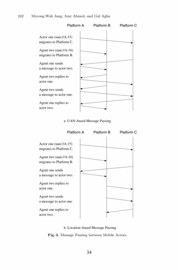
242 Myeong-Wuk Jang, Amr Ahmed, and Gul Agha

b. Location−based Message Passing

Platform A Platform B Platform C

a. UAN−based Message Passing

Platform A Platform B Platform C

Actor one (uan://A:15) migrates to Platform C.

Agent two (uan://A:16) migrates to Platform B.

Agent one sends a message to actor two.

Agent two replies toactor one.

a message to actor one.Agent two sends

Agent one replies toactor two.

Actor one (uan://A:15) migrates to Platform C.

Agent two (uan://A:16) migrates to Platform B.

Agent one sends a message to actor two.

Agent two replies toactor one.

a message to actor one.Agent two sends

Agent one replies toactor two.

Fig. 3. Message Passing between Mobile Actors.

34

Efficient Agent Communication in Multi-agent Systems 243

message with its LAN to update its location at the sender actor. Therefore, thesender actor can use the updated information for subsequent messages.

3.2 Delayed Message Passing

While a mobile actor is moving from one AA platform to another, the current AAplatform of the actor is not well defined. In AA, because the location informationof a mobile actor is updated after it finishes migration, its original AA platformthinks the actor still exists on its old AA platform during migration. Therefore,when the Message Manager of the original AA platform receives a message fora mobile actor, it sends the message to the Message Manager of the old AAplatform thinking that it is still there. After the Message Manager of the old AAplatform receives the message, it forwards the message to the Message Managerof the original AA platform. Thus, a message is continuously passed betweenthese two AA platforms until the mobile actor updates the Actor Manager of itsoriginal AA platform with its new location.

In order to avoid unnecessary message thrashing, we use the Delayed MessageManager in each AA platform. After the actor starts its migration, the ActorManager of the old AA platform changes its state to be Transit. From thismoment, the Delayed Message Manager of this platform holds messages for thismobile actor until the actor reports that its migration has ended. After the mobileactor finishes its migration, its new AA platform sends its old AA platform andits original AA platform a message to inform them that the migration processhas ended. When these two AA platforms receive this message, the original AAplatform changes the state of the mobile actor from Transit to Remote whilethe old AA platform removes all information about the mobile actor, and theDelayed Message Manager of the old AA platform forwards the delayed messagesto the Message Manager of the new AA platform of the actor.

4 Active Brokering Service

An ATSpace supports active brokering services by allowing agents to send theirown search algorithms to be executed in the ATSpace address space [14]. Wecompare this service to current middle agent services.

Many middle agents are based on attribute-based communication. Serviceagents register themselves with the middle agent by sending a tuple whose at-tributes describe the service they advertise. To find the desired service agents, aclient agent supplies a tuple template with constraints on attributes. The middleagent then tries to find service agents whose registered attributes match the sup-plied constraints. Systems vary more or less according to the types of constraints(primitives) they support. Typically, a middle agent provides exact matching orregular expression matching [2, 11, 17]. As we mentioned earlier, this solutionsuffers from a lack of expressiveness and incomplete information.

For example, consider a middle agent with information about seller agents.Each service agent (seller) advertises itself with the following attributes <actor

35

244 Myeong-Wuk Jang, Amr Ahmed, and Gul Agha

name, seller city, product name, product price>. A client agent with thefollowing query is stuck:

Q1: What are the best two (in terms of price) sellers that offer computers andwhose locations are roughly within 50 miles of me?

Considering the current tuple space technology, the operator “best two” isclearly not supported (expressiveness problem). Morever, the tuple space doesnot include distance information between cities (incomplete information prob-lem). Faced with these difficulties, a user with this complex query Q1 has totransform it into a simpler one that is accepted by the middle agent which re-trieves a superset of the data to be retrieved by Q1. In our example, a simplerquery could be:

Q2: Find all tuples about sellers that sell computers.

An apparent disadvantage of the above approach is the movement of a largeamount of data from the middle agent space to the buyer agent, especially if Q2is semantically distant from Q1. In order to reduce communication overhead,ATSpace allows a sender agent to send its own search algorithm to find serviceagents, and the algorithm is executed in the ATSpace. In our example, the buyeragent would send a search object that would inspect tuples in the middle agentand select the best two sellers that satisfy the buyer criteria.

4.1 Security Issues

Although active brokering services mitigate the limitations of middle agents, suchas brokers or matchmakers, they also introduce the following security problemsin ATSpaces:

– Data Integrity: A search object may not modify tuples owned by other actors.– Denial of Service: A search object may not consume too much processing

time or space of an ATSpace, and a client actor may not repeatedly sendsearch objects to overload an ATSpace.

– Illegal Access : A search object may not carry out unauthorized accesses orillegal operations.

We address the first problem by preventing the search object from modifyingtuple data of other actors. This is done by supplying methods of the search objectwith a copy of the data in the ATSpace. However, when the number of tuplesin the ATSpace is large, this solution requires extra memory and computationresources. Thus the ATSpace supports the option of delivering a shallow copyof the original tuples to the search object at the risk of data being changed bysearch objects as such scheme may compromise the data integrity.

To prevent malicious objects from exhausting the ATSpace computationalresource, we deploy user-level thread scheduling as depicted in Fig. 4. Whena search object arrives, the object is executed as a thread and its priority is

36

Efficient Agent Communication in Multi-agent Systems 245

job queues

priority

priorityhigh

priority

low

middle

Tuple Space Tuple Space Manager

ATSpaceManager

ATSpace

tuple

tuple

tuple

obj.obj.

obj.obj.

obj.obj.

tuple

Fig. 4. Architecture of an ATSpace.

set to high. If the thread executes for a long time, its priority is continuouslydowngraded. Moreover, if the running time of a search object exceeds a certainlimit, it may be destroyed by the tuple space manager.

To prevent unauthorized accesses, if the ATSpace is created with an accesskey, then this key must accompany every message sent from client actors. In thiscase, actors are allowed only to modify their own tuples. This prevents removalor modification of tuples by unauthorized actors.

5 Experiments and Evaluation

The AA platforms and actors have been implemented in Java language to sup-port operating system independent actor mobility. The Actor Architecture isbeing used for large-scale UAV (Unmanned Aerial Vehicle) simulations. Thesesimulations investigate the effects of different collaborative behaviors among alarge number of micro UAVs during their surveillance missions over a large num-ber of moving targets [15]. For our experiments, we have tested more than 1,000actors on four computers: 500 micro UAVs, 500 targets, and other simulationpurpose actors are executed. The following two sections evaluate our solutions.

5.1 Optimized Message Delivery

According to our experiments, the location-based message passing scheme in AAreduces the number of hops (over AA platforms) that a message for a mobileactor goes through. Since an agent has the location information about its col-laborating agents, the agent can carry this information when it moves from oneAA platform to another. With location-based message passing, the system ismore fault-tolerant; since messages for a mobile actor need not pass through theoriginal AA platform of the actor, the messages may be correctly delivered tothe actor even when the actor’s original AA platform is not working correctly.

37

246 Myeong-Wuk Jang, Amr Ahmed, and Gul Agha

Moreover, delayed message passing removes unnecessary message thrashingfor moving agents. When delayed message passing is used, the old AA platformof a mobile actor needs to manage its state information until the actor finishesits migration, and the new platform of the mobile actor needs to report themigration state of the actor to its old AA platforms. In our experiments, thisoverhead is more than compensated; without delayed message passing the samemessage may get delivered seven or eight times between the original AA platformand the old AA platform while a mobile actor is moving. If a mobile actor takesmore time for its migration, this number may be even greater.

5.2 Active Brokering Service

The performance benefit of ATSpace can be measured by comparing its activebrokering services with the data retrieval services of a template-based generalmiddle agent supporting the same service along four different dimensions: thenumber of messages, the total size of messages, the total size of memory spaceon the client and middle agent AA platforms, and the computation time for thewhole operation. To analytically evaluate ATSpaces, we will use the scenariomentioned in section 4 where a service requesting agent has a complex querythat is not supported by the template-based model.

First, with the template-based service, the number of messages is n+2 wheren is the number of service agents that satisfy a complex query. This is because theservice requesting agent has to first send a message to the middle agent to bring asuperset of its final result. This costs two messages: a service request message tothe middle agent (Service Requesttemplate) that contains Q2 and a reply mes-sage that contains agent information satisfying Q2 (Service Replytemplate).Finally, the service requesting agent sends n messages to the service agents thatmatch its original criteria. With the active brokering service, the total numberof messages is n+1. This is because the service requesting agent need not worryabout the complexity of his query and only sends a service request message(Service RequestATSpace) to the ATSpace. This message contains the codethat represents its criteria along with the message that should be sent to theagents which satisfy these criteria. The last n messages have the same explana-tion as in the template-based service.

While the number of messages in the two approaches does not differ thatmuch, the total size of these messages may have a huge difference. In bothapproaches, a set of n messages needs to be sent to the agents that satisfy thefinal matching criteria. Therefore, the question of whether or not active brokeringservices result in bandwidth saving depends on the relative size of the othermessages. Specifically the difference in bandwidth consumption (DBC ) betweenthe template-based middle agent and the ATSpace is given by the followingequation:

DBC = [size(Service Requesttemplate) −size(Service RequestATSpace)] +

size(Service Replytemplate)

38

Efficient Agent Communication in Multi-agent Systems 247

In general, since the service request message in active brokering services islarger as it has the search object, the first component is negative. Therefore,active brokering services will only result in a bandwidth saving if the increase inthe size of its service request message is smaller than the size of the service replymessage in the template-based service. This is likely to be true if the originalquery (Q1) is complex such that turning it into a simpler one (Q2) to retrievea superset of the result would incur a great semantic loss and as such wouldretrieve much extra agent information from the middle agent.

Third, the two approaches put a conflicting requirement on the amount ofspace needed on both the client and middle agent machines. In the template-based approach the client agent needs to provide extra space to store the tuplesreturned by Q2. On the hand, the ATSpace needs to provide extra space to storecopies of tuples given to search objects. However, a compromise can be madehere as the creator of the ATSpace can choose to use the shallow copy of tuples.

Fourth, the difference in computation times of the whole operation in the twoapproaches depends on two factors: the time for sending messages and the timefor evaluating queries on tuples. The tuples in the ATSpace are only inspectedonce by the search object sent by the service requesting agent. However, in thetemplate-based middle agent, some tuples are inspected twice. First, in orderto evaluate Q2, the middle agent needs to inspect all the tuples that it has.Second, these tuples that satisfy Q2 are sent back to the service requestingagent to inspect them again and retain only those tuples that satisfy Q1. If Q1is complex then Q2 will be semantically distant from Q1, which in turns has tworamifications. First, the time to evaluate Q2 against all the tuples in the middleagent is small relative to the time needed to evaluate the search object over them.Second, most of the tuples on the middle agent would pass Q2 and be sent backto be re-evaluated by the service requesting agent. This reevaluation has nearlythe same complexity as running the search object code. Thus we conclude thatwhen the original query is complex and external communication cost is high, theactive brokering service will result in time saving.

Apart from the above analytical evaluation, we have run a series of experi-ments on the UAV simulation to substantiate our claims. (Interested readers mayrefer to [13] for more details.) Fig. 5 demonstrates the saving in computationaltime of an ATSpace compared to a template-based middle agent that providesdata retrieval services with the same semantic. Fig. 6 shows the wall clock timeratio of a template-based middle agent to an ATSpace. In these experiments,UAVs use either active brokering services or data retrieval services to find theirneighboring UAVs. In both cases, the middle agent includes information aboutlocations of UAVs and targets. In case of the active brokering service, UAVs sendsearch objects to an ATSpace while the UAVs using data retrieval service sendtuple templates. The simulation time for each run is around 35 minutes, and thewall clock time depends on the number of agents. When the number of agentsis small, the difference between the two approaches is not significant. However,as the number of agents is increased, the difference becomes large.

39

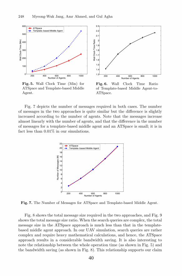
248 Myeong-Wuk Jang, Amr Ahmed, and Gul Agha

200 400 600 800 10000

100

200

300

400

500

600

Number of Agents

Wal

l Clo

ck T

ime

(Min

)

ATSpaceTemplate−based Middle Agent

Fig. 5. Wall Clock Time (Min) forATSpace and Template-based MiddleAgent.

200 400 600 800 10001.3

1.4

1.5

1.6

1.7

1.8

1.9

2

2.1

2.2

2.3

Number of Agents

Wal

l Clo

ck T

ime

Rat

io

Fig. 6. Wall Clock Time Ratioof Template-based Middle Agent-to-ATSpace.

Fig. 7 depicts the number of messages required in both cases. The numberof messages in the two approaches is quite similar but the difference is slightlyincreased according to the number of agents. Note that the messages increasealmost linearly with the number of agents, and that the difference in the numberof messages for a template-based middle agent and an ATSpace is small; it is infact less than 0.01% in our simulations.

200 400 600 800 10000

2

4

6

8

10

12

14

16

18

20

22

Number of Agents

Num

ber

of M

essa

ges

(M)

ATSpaceTemplate−based Middle Agent

Fig. 7. The Number of Messages for ATSpace and Template-based Middle Agent.

Fig. 8 shows the total message size required in the two approaches, and Fig. 9shows the total message size ratio. When the search queries are complex, the totalmessage size in the ATSpace approach is much less than that in the template-based middle agent approach. In our UAV simulation, search queries are rathercomplex and require heavy mathematical calculations, and hence, the ATSpaceapproach results in a considerable bandwidth saving. It is also interesting tonote the relationship between the whole operation time (as shown in Fig. 5) andthe bandwidth saving (as shown in Fig. 8). This relationship supports our claim

40

Efficient Agent Communication in Multi-agent Systems 249

200 400 600 800 10000

5

10

15

20

25

30

35

Number of Agents

Tot

al S

ize

of M

essa

ges

(GB

ytes

)

ATSpaceTemplate−based Middle Agent

Fig. 8. Total Message Size (GBytes)for ATSpace and Template-basedMiddle Agent.

200 400 600 800 10001.2

1.3

1.4

1.5

1.6

1.7

1.8

Number of Agents

Tot

al S

ize

of M

essa

ge R

atio

Fig. 9. Total Message Size Ratiofor Template-based Middle Agent-to-ATSpace.

that the saving in the total operation time by the ATSpace is largely due to itssuperiority in efficiently utilizing the bandwidth.

6 Related Work

The basic mechanism of location-based message passing is similar to the mes-sage passing in Mobile IP [20], although its application domain is different. Theoriginal and current AA platforms of a mobile actor correspond to the home andforeign agents of a mobile client in Mobile IP, and the UAN and LAN of a mo-bile actor are similar to the home address and care-of address of a mobile clientin Mobile IP. However, while the sender node in Mobile IP manages a bindingcache to map home addresses to care-of addresses, the sender AA platform inAA does not have a mapping table. Another difference is that in mobile IP, thehome agent communicates with the sender node to update the binding cache.However, in AA this update can be done by the agent itself when it sends amessage that contains its address.

The LAN (Location-based Actor Name) may also be compared to UAL (Uni-versal Actor Locator) in SALSA [27]. In SALSA, UAL represents the location ofan actor. However, SALSA uses a middle agent called Universal Actor NamingServer to locate the receiver actor. SALSA’s approach requires the receiver ac-tor to register its location at a certain middle agent, and the middle agent mustmanage the mapping table.

The ATSpace approach, which is based on the tuple space model, is relatedto Linda [6]. In the Linda model, processes communicate with other processesthrough a shared common space called a blackboard or a tuple space withoutconsidering references or names of other processes [6, 21]. This approach was usedin several agent frameworks, for example EMAF [3] and OAA [8]. However, thesemodels support only primitive features for pattern-based communication amongprocesses or agents. From the middle agent perspective, Directory Facilitator in

41

250 Myeong-Wuk Jang, Amr Ahmed, and Gul Agha

the FIPA platform [10], ActorSpace [2], and Broker Agent in InfoSleuth [16] arerelated to our research. However, these systems do not support customizablematching algorithms.

From the expressiveness perspective, some work has been done to extendthe matching capability of the basic tuple space model. Berlinda [26] allows aconcrete entry class to extend the matching function, and TS [12] uses policyclosures in a Scheme-like language to customize the behavior of tuple spaces.However, these approaches do not allow the matching function to be changedduring execution time. At the other hand, OpenSpaces [9] provides a mechanismto change matching polices during the execution time. OpenSpaces groups en-tries in its space into classes and allows each class to have its individual matchingalgorithm. A manager for each class of entries can change the matching algo-rithm during execution time. All agents that use entries under a given class areaffected by any change to its matching algorithm. This is in contrast to theATSpace where each agent can supply its own matching algorithm without af-fecting other agents. Another difference between OpenSpaces and ATSpaces isthat the former requires a registration step before putting the new matchingalgorithm into action, but ATSpace has no such requirement.

Object Space [22] allows distributed applications implemented in the C++programming language to use a matching function in its template. This matchingfunction is used to check whether an object tuple in the space is matched with thetuple template given in rd and in operators. However, in the ATSpace the clientagent supplied search objects can have a global overview of the tuples storedin the shared space and hence can support global search behavior rather thanthe one tuple based matching behavior supported in Object Space. For example,using the ATSpace a client agent can find the best ten service agents accordingto its criteria whereas this behavior cannot be achieved in Object Space.

TuCSoN [19] and MARS [5] provide programmable coordination mechanismsfor agents through Linda-like tuple spaces to extend the expressive power of tu-ple spaces. However, they differ in the way they approach the expressivenessproblem; while TuCSoN and MARS use reactive tuples to extend the expres-sive power of tuple spaces, the ATSpace uses search objects to support searchalgorithms defined by client agents. A reactive tuple handles a certain type oftuples and affects various clients, whereas a search object handles various typesof tuples and affects only its creator agent. Therefore, while TuCSoN and MARSextend the general search ability of middle agents, ATSpace supports applicationagent-oriented searching on middle agents.

Mobile Co-ordination [23] allows agents to move a set of multiple tuple spaceaccess primitives to a tuple space for fault tolerance. In Jada [7], one primitivemay use multiple matching templates. In ObjectPlaces [24], dynamic objects areused to change their state whenever corresponding objecplace operations arebeing called. Although these approaches improve the searching ability of tuplespaces with a set of search templates or dynamic objects, ATSpace providesmore flexibility to application agents with their own search code.

42

Efficient Agent Communication in Multi-agent Systems 251

7 Conclusion and Future Work

In this papers we addressed two closely related agent communication issues: effi-cient message delivery and service agent discovery. Efficient message delivery hasbeen addressed using two techniques. First, the agent naming scheme has beenextended to include the location information of mobile agents. Second, messageswhose destination agent is moving are postponed by the Delayed Message Man-ager until the agent finishes its migration. For efficient service agent discovery,we have addressed the ATSpace, Active Tuple Space. By allowing applicationagents to send their customized search algorithms to the ATSpace, applicationagents may efficiently find service agents. We have synthesized our solutions tothe mobile agent addressing and service agent discovery problems in a multi-agent framework.

The long term goal of our research is to build an environment that allows forexperimental study of various issues that pertains to message passing and ser-vice agent discovery in open multi-agent systems and provide a principled wayof studying possible tensions that arise when trying to simultaneously optimizeeach service. Other future directions include the followings: for efficient messagepassing, we plan to investigate various trade-offs in using different message pass-ing schemes for different situations. We also plan to extend the Delayed MessageManager to support mobile agents who are contiguously moving between nodes.For service agent discovery, we plan to elaborate on our solutions to the securityissues introduced with active brokering services.

Acknowledgements

The authors would like to thank the anonymous reviewers and Naqeeb Abbasifor their helpful comments and suggestions. This research is sponsored by theDefense Advanced Research Projects Agency under contract number F30602-00-2-0586.

References

1. G. Agha. Actors: A Model of Concurrent Computation in Distributed Systems.MIT Press, 1986.

2. G. Agha and C.J. Callsen. ActorSpaces: An Open Distributed ProgrammingParadigm. In Proceedings of the 4th ACM Symposium on Principles and Prac-tice of Parallel Programming, pages 23–32, May 1993.

3. S. Baeg, S. Park, J. Choi, M. Jang, and Y. Lim. Cooperation in MultiagentSystems. In Intelligent Computer Communications (ICC ’95), pages 1–12, Cluj-Napoca, Romania, June 1995.

4. F. Bellifemine, A. Poggi, and G. Rimassa. JADE - A FIPA-compliant AgentFramework. In Proceedings of Practical Application of Intelligent Agents and Multi-Agents (PAAM ’99), pages 97–108, London, UK, April 1999.

5. G. Cabri, L. Leonardi, and F. Zambonelli. MARS: a Programmable CoordinationArchitecture for Mobile Agents. IEEE Computing, 4(4):26–35, 2000.

43

252 Myeong-Wuk Jang, Amr Ahmed, and Gul Agha

6. N. Carreiro and D. Gelernter. Linda in Context. Communications of the ACM,32(4):444–458, 1989.

7. P. Ciancarini and D. Rossi. Coordinating Java Agents over the WWW. WorldWide Web, 1(2):87–99, 1998.

8. P.R. Cohen, A.J. Cheyer, M. Wang, and S. Baeg. An Open Agent Architecture.In AAAI Spring Symposium, pages 1–8, March 1994.

9. S. Ducasse, T. Hofmann, and O. Nierstrasz. OpenSpaces: An Object-OrientedFramework for Reconfigurable Coordination Spaces. In A. Porto and G.C. Roman,editors, Coordination Languages and Models, LNCS 1906, pages 1–19, Limassol,Cyprus, September 2000.

10. Foundation for Intelligent Physical Agents. SC00023J: FIPA Agent ManagementSpecification, December 2002. http://www.fipa.org/specs/fipa00023/.

11. N. Jacobs and R. Shea. The Role of Java in InfoSleuth: Agent-based Exploita-tion of Heterogeneous Information Resources. In Proceedings of Intranet-96 JavaDevelopers Conference, April 1996.

12. S. Jagannathan. Customization of First-Class Tuple-Spaces in a Higher-Order Lan-guage. In Proceedings of the Conference on Parallel Architectures and Languages- Vol. 2, LNCS 506, pages 254–276. Springer-Verlag, 1991.

13. M. Jang, A. Ahmed, and G. Agha. A Flexible Coordination Framework forApplication-Oriented Matchmaking and Brokering Services. Technical ReportUIUCDCS-R-2004-2430, Department of Computer Science, University of Illinoisat Urbana-Champaign, 2004.

14. M. Jang, A. Abdel Momen, and G. Agha. ATSpace: A Middle Agent to SupportApplication-Oriented Matchmaking and Brokering Services. In IEEE/WIC/ACMIAT(Intelligent Agent Technology)-2004, pages 393–396, Beijing, China, September20-24 2004.

15. M. Jang, S. Reddy, P. Tosic, L. Chen, and G. Agha. An Actor-based Simulationfor Studying UAV Coordination. In 15th European Simulation Symposium (ESS2003), pages 593–601, Delft, The Netherlnds, October 26-29 2003.

16. R.J. Bayardo Jr., W. Bohrer, R. Brice, A. Cichocki, J. Fowler, A. Helal,V. Kashyap, T. Ksiezyk, G. Martin, M. Nodine, M. Rashid, M. Rusinkiewicz,R. Shea, C. Unnikrishnan, A. Unruh, and D. Woelk. InfoSleuth: Agent-BasedSemantic Integration of Information in Open and Dynamic Environments. ACMSIGMOD Record, 26(2):195–206, June 1997.

17. D.L. Martin, H. Oohama, D. Moran, and A. Cheyer. Information Brokering inan Agent Architecture. In Proceedings of the Second International Conference onthe Practical Application of Intelligent Agents and Multi-Agent Technology, pages467–489, London, April 1997.

18. D.G.A. Mobach, B.J. Overeinder, N.J.E. Wijngaards, and F.M.T. Brazier. Man-aging Agent Life Cycles in Open Distributed Systems. In Proceedings of the 2003ACM symposium on Applied Computing, pages 61–65, Melbourne, Florida, 2003.

19. A. Omicini and F. Zambonelli. TuCSoN: a Coordination Model for Mobile In-formation Agents. In Proceedings of the 1st Workshop on Innovative InternetInformation Systems, Pisa, Italy, June 1998.

20. C.E. Perkins. Mobile IP. IEEE Communications Magazine, 35:84–99, May 1997.21. K. Pfleger and B. Hayes-Roth. An Introduction to Blackboard-Style Systems Orga-

nization. Technical Report KSL-98-03, Stanford Knowledge Systems Laboratory,January 1998.

22. A. Polze. Using the Object Space: a Distributed Parallel make. In Proceedingsof the 4th IEEE Workshop on Future Trends of Distributed Computing Systems,pages 234–239, Lisbon, September 1993.

44

Efficient Agent Communication in Multi-agent Systems 253

23. A. Rowstron. Mobile Co-ordination: Providing Fault Tolerance in Tuple SpaceBased Co-ordination Languages. In Proceedings of the Third International Con-ference on Coordination Languages and Models, pages 196–210, 1999.

24. K. Schelfthout and T. Holvoet. ObjectPlaces: An Environment for Situated Multi-Agent Systems. In Third International Joint Conference on Autonomous Agentsand Multiagent Systems - Volume 3 (AAMAS’04), pages 1500–1501, New YorkCity, New York, July 2004.

25. K. Sycara, K. Decker, and M. Williamson. Middle-Agents for the Internet. InProceedings of the 15th Joint Conference on Artificial Intelligences (IJCAI-97),pages 578–583, 1997.

26. R. Tolksdorf. Berlinda: An Object-oriented Platform for Implementing Coordi-nation Language in Java. In Proceedings of COORDINATION ’97 (CoordinationLanguages and Models), LNCS 1282, pages 430–433. Pringer-Verlag, 1997.

27. C.A. Varela and G. Agha. Programming Dynamically Reconfigurable Open Sys-tems with SALSA. ACM SIGPLAN Notices: OOPSLA 2001 Intriguing TechnologyTrack, 36(12):20–34, December 2001.

28. M. Wooldridge. An Introduction to MultiAgent Systems. John Wiley & Sons, Ltd,2002.

45

Software Tools for Technology Transfer manuscript No.(will be inserted by the editor)

Online Efficient Predictive Safety Analysis of MultithreadedPrograms

Koushik Sen and Grigore Rosu and Gul AghaDepartment of Computer Science,University of Illinois at Urbana-Champaign.ksen,grosu,agha@cs.uiuc.edu

Received: date / Revised version: date

Abstract. We present an automated and configurabletechnique for runtime safety analysis of multithreadedprograms which is able to predict safety violations fromsuccessful executions. Based on a formal specification ofsafety properties that is provided by a user, our tech-nique enables us to automatically instrument a givenprogram and create an observer so that the programemits relevant state update events to the observer andthe observer checks these updates against the safetyspecification. The events are stamped with dynamic vec-tor clocks, enabling the observer to infer a causal partialorder on the state updates. All event traces that areconsistent with this partial order, including the actualexecution trace, are then analyzed online and in para-llel. A warning is issued whenever one of these potentialtrace violates the specification. Our technique is scal-able and can provide better coverage than conventionaltesting but its coverage need not be exhaustive. In fact,one can trade-off scalability and comprehensiveness: awindow in the state space may be specified allowing theobserver to infer some of the more likely runs; if the sizeof the window is 1 then only the actual execution traceis analyzed, as is the case in conventional testing; if thesize of the window is ∞ then all the execution tracesconsistent with the actual execution trace are analyzed.

1 Introduction

In multithreaded systems, threads can execute concur-rently communicating with each other through a set ofshared variables, yielding an inherent potential for sub-tle errors due to unexpected interleavings. Both rigor-ous and light-weight techniques to detect errors in mul-tithreaded systems have been extensively investigated.Rigorous techniques include formal methods, such as

model checking and theorem proving, which by exploring–directly or indirectly– all possible thread interleavings,guarantee that a formal model of the system satisfies itssafety requirements. Unfortunately, despite impressiverecent advances, the size of systems for which modelchecking or automatic theorem proving is feasible re-mains rather limited. As a result, most system builderscontinue to use light-weight techniques such as testingto identify bugs in their implementations.

There are two problems with software testing. First,testing is generally done in an ad hoc manner: the soft-ware developer must hand-translate the requirementsinto specific dynamic checks on the program state. Sec-ond, test coverage is often rather limited, covering onlysome execution paths: if an error is not exposed by a par-ticular test case then that error is not detected. To mit-igate the first problem, software often includes dynamicchecks on a system’s state in order to identify problemsat run-time. To ameliorate the second problem, manytechniques increase test coverage by developing test-casegeneration methods that generate test cases which mayreveal potential errors with high probability [6,15,26].

Based on experience with related techniques andtools, namely Java PathExplorer (JPaX) [12] andits sub-system Eagle [2], we have proposed in [22,23]an alternative approach, called predictive runtime anal-ysis. The essential idea of this analysis technique is asfollows. Suppose that a multithreaded program has asafety error, such as a violation of a temporal property,a deadlock, or a data-race. As in testing, we execute theprogram on some carefully chosen input (a test case).Suppose that the error is not revealed during a par-ticular execution, i.e., the execution is successful withrespect to that bug. If one regards the execution of aprogram as a flat, sequential trace of events or states,as in NASA’s JPaX system [12], University of Pennsyl-vania’s Java-MaC [14], Bell Labs’ PET [11], Nokia’sThird Eye framework [16] inspired by Logic Assurance

46

2 K. Sen and G. Rosu and G. Agha: Online Efficient Predictive Safety Analysis of Multithreaded Programs

system [24], or the commercial analysis systems Tempo-ral Rover and DBRover [7–9], then there is not much leftto do to find the error except to run another, hopefullybetter, test case. However, by observing the executiontrace in a smarter way, namely as a causal dependencypartial order on state updates, we can predict errors thatmay potentially occur in other possible runs of the mul-tithreaded program.

Our technique merges testing and formal methodsto obtain some of the advantages of both while avoid-ing the pitfalls of ad hoc testing and the complexity offull-blown formal verification. Specifically, we develop aruntime verification technique for safety analysis of mul-tithreaded systems that can be tuned to analyze a num-ber of traces that are consistent with an actual executionof the program. Two extreme instances of our techniqueinvolve checking all or one of the variant traces:

– If all traces are checked then it becomes equivalentto online model checking of an abstract model of theprogram, called the multithreaded computation lat-tice, extracted from the actual execution trace of theprogram, like in POTA [19] or JMPaX [22].

– If only one trace is considered, then our techniquebecomes equivalent to checking just the actual exe-cution of the multithreaded program, as is done intesting or like in other runtime analysis tools likeMaC [14] and PaX [12,2].

In general, depending on the application, one canconfigure a window within the state space to be exploredwhich, intuitively speaking, provides a causal distancefrom the observed execution within which all traces areexhaustively verified. We call such a window a causalitycone. An appealing aspect of our technique is that allthese traces can be analyzed online, as the events arereceived from the running program, and in parallel. Theworst case cost of such an analysis is proportional toboth the size of the window and the size of the statespace of the monitor.

There are three important interrelated componentsin our runtime verification technique. Our algorithm syn-thesizes these components automatically from the safetyspecification:

Instrumentor. The code instrumentor, based on thesafety specification, entirely automatically adds codeto emit events when relevant state updates occur.

Observer. The observer receives the events from the in-strumented program as they are generated, enqueuesthem and then builds a configurable abstract modelof the system, known as a computation lattice, on alayer-by-layer basis.

Monitor. As layers are completed, the monitor checksthem against the safety specification and then dis-cards them.

The concepts and notions presented in this paperhave been experimented and tested on JMPaX 2.0, a

prototype monitoring system for Java programs that wehave built. JMPaX 2.0 extends its predecessor JMPaXin at least four non-trivial novel ways:

– The technical notion of dynamic vector clock is in-troduced, which allows us to properly deal with thedynamic creation and destruction of threads.

– The variables that are shared between threads neednot be static: an automatic instrumentation tech-nique has been devised that detects automaticallywhen a variable is shared.

– The notion of cone heuristic, or global state window,is introduced. The cone heuristic enables us to in-crease the runtime efficiency by analyzing the mostlikely states in the computation lattice and tune howcomprehensive we wish to be.

– The runtime prediction paradigm used is indepen-dent of the safety formalism, in the sense that it al-lows the user to specify any safety property whosebad prefixes can be expressed as a non-deterministicfinite automaton (NFA).

Part of this work was presented at the 10th InternationalConference on Tools and Algorithms for the Construc-tion and Analysis of Systems (TACAS’04) [23].

2 Monitors for Safety Properties

Safety properties are a very important, if not the mostimportant, class of properties that one should considerin monitoring. This is because once a system violatesa safety property, there is no way to continue its exe-cution to satisfy the safety property later. Therefore, amonitor for a safety property can precisely say at run-time when the property has been violated, so that anexternal recovery action can be taken. From a monitor-ing perspective, what is needed from a safety formula isa succinct representation of its bad prefixes, which arefinite sequences of states leading to a violation of theproperty. Therefore, one can abstract away safety prop-erties by languages over finite words.

Automata are a standard means to succinctly rep-resent languages over finite words. In what follows wedefine a suitable version of automata, called monitor,with the property that it has a “bad” state from whichit never gets out:

Definition 1. Let S be a finite or infinite set, that canbe thought of as the set of states of the program to bemonitored. Then an S-monitor or simply a monitor, isa tuple Mon = 〈M,m0, b, ρ〉, where

– M is the set of states of the monitor;– m0 ∈M is the initial state of the monitor;– b ∈ M is the final state of the monitor, also called

bad state; and

47

K. Sen and G. Rosu and G. Agha: Online Efficient Predictive Safety Analysis of Multithreaded Programs 3

– ρ : M × S → 2M is a non-deterministic transitionrelation with the property that ρ(b,Σ) = b for anyΣ ∈ S.

Sequences in S?, where ε is the empty one, are called(execution) traces. A trace π is said to be a bad prefixin Mon iff b ∈ ρ(m0, π), where ρ : 2M × S? → 2M

is recursively defined as ρ(M, ε) = M and ρ(M, πΣ) =ρ(ρ(M,π), Σ), where ρ : 2M × S → 2M is defined asρ(m ∪ M, Σ) = ρ(m,Σ) ∪ ρ(M, Σ) and ρ(∅, Σ) = ∅,for all finite M ⊆M and Σ ∈ S.

M is not required to be finite in the above definition,but 2M represents the set of finite subsets of M. Inpractical situations it is often the case that the monitor isnot explicitly provided in a mathematical form as above.For example, a monitor can be a specific type of programwhose execution is triggered by receiving events fromthe monitored program; its state can be given by thevalues of its local variables, and the bad state is a fixedunique state which once reached cannot be changed byany further events.

There are fortunate situations in which monitors canbe automatically generated from formal specifications,thus requiring the user to focus on system’s formal safetyrequirements rather than on low level implementationdetails. In fact, this was the case in all the experimentsthat we have performed so far. We have so far experi-mented with requirements expressed either in extendedregular expressions (ERE) or various variants of tempo-ral logics, with both future and past time. For example,[20,21] show coinductive techniques to generate mini-mal static monitors from EREs and from future timelinear temporal logics, respectively, and [13,2] show howto generate dynamic monitors, i.e., monitors that gen-erate their states on-the-fly, as they receive the events,for the safety segment of temporal logic. Note, however,that there may be situations in which the generation ofa monitor may not be feasible, even for simple require-ments languages. For example, it is well-known that theequivalent automaton of an ERE may be non-elementarylarger in the worst case [25]; therefore, there exist rela-tively small EREs whose monitors cannot even be stored.

Example 1. Consider a reactive controller that main-tains the water level of a reservoir within safe bounds. Itconsists of a water level reader and a valve controller.The water level reader reads the current level of thewater, calculates the quantity of water in the reservoirand stores it in a shared variable w. The valve controllercontrols the opening of a valve by looking at the cur-rent quantity of water in the reservoir. A very simpleand naive implementation of this system contains twothreads: T1, the valve controller, and T2, the water levelreader. The code snippet is given in Fig. 1.

Here w is in some proper units such as mega gallonsand v is in percentage. The implementation is poorlysynchronized and it relies on ideal thread scheduling.

Thread T1: Thread T2:

while(true) while(true) if(w > 18) delta = 10; l = readLevel();

else delta = -10; w = calcVolume(l);

for(i=0; i<2; i++) sleep(100);

v = v + delta; setValveOpening(v);

sleep(100);

5

0

1

~p

2

p,~q

q,~r

p,~q

3

p,~q,~r

4

q

q

p,~q

q,~r

q

Fig. 1. Two threads (T1 controls the valve and T2 reads the waterlevel) and a monitor.

A sample run of the system can be w = 20, v =40, w = 24, v = 50, w = 27, v = 60, w =31, v = 70. As we will see later in the paper, by arun we here mean a sequence of relevant variable writes.Suppose we are interested in a safety property that says“If the water quantity is more than 30 mega gallons, thenit is the case that sometime in the past water quantityexceeded 26 mega gallons and since then the valve isopen by more than 55% and the water quantity neverwent down below 26 mega gallon”. We can express thissafety property in two different formalisms: linear tem-poral logic (LTL) with both past-time and future-timeoperators, or extended regular expressions (EREs) forbad prefixes. The atomic propositions that we will con-sider are p : (w > 26), q : (w > 30), r : (v > 55). Theproperties can be written as follows:

F1 = ¤(q → ((r ∧ p)S ↑p))F2 = ∗¬pp,¬q+

(p,¬q,¬rp,¬q∗q+ q∗q,¬r)∗

The formula F1 in LTL (↑ p is a shorthand for “pand previously not p”) states that “It is always the casethat if (w > 30) then at some time in the past (w > 26)started to be true and since then (r > 55) and (w > 26).”

48

4 K. Sen and G. Rosu and G. Agha: Online Efficient Predictive Safety Analysis of Multithreaded Programs

The formula F2 characterizes the prefixes that make F1

false. In F2 we use p,¬q to denote a state where p and¬q holds and r may or may not hold. Similarly, rep-resents any state of the system. The monitor automatonfor F2 is given also in Fig. 1.

3 Multithreaded Programs

We consider multithreaded systems in which threadscommunicate with each other via shared variables. Acrucial point is that some variable updates can causallydepend on others. We will describe an efficient dynamicvector clock algorithm which, given an executing multi-threaded program, generates appropriate messages to besent to an external observer. Section 4 will show how theobserver, in order to perform its more elaborated anal-ysis, extracts the state update information from suchmessages together with the causality partial order.

3.1 Multithreaded Executions and Shared Variables

A multithreaded program consists of n threads t1, t2, ...,tn that execute concurrently and communicate with eachother through a set of shared variables. A multithreadedexecution is a sequence of events e1e2 . . . er generated bythe running multithreaded program, each belonging toone of the n threads and having type internal, read orwrite of a shared variable. We use ej

i to represent thejth event generated by thread ti since the start of itsexecution. When the thread or position of an event isnot important we can refer to it generically, such as e,e′, etc.; we may write e ∈ ti when event e is generatedby thread ti. Let us fix an arbitrary but fixed multi-threaded execution, say C, and let S be the set of allvariables that were shared by more than one thread inthe execution. There is an immediate notion of variableaccess precedence for each shared variable x ∈ S: we saye x-precedes e′, written e <x e′, iff e and e′ are variableaccess events (reads or writes) to the same variable x,and e “happens before” e′, that is, e occurs before e′ inC. This can be realized in practice by keeping a counterfor each shared variable, which is incremented at eachvariable access.

3.2 Causality and Multithreaded Computations

Let E be the set of events occurring in C and let ≺ bethe partial order on E :

– eki ≺ el

i if k < l;– e ≺ e′ if there is x ∈ S with e <x e′ and at least one

of e, e′ is a write;– e ≺ e′′ if e ≺ e′ and e′ ≺ e′′.

We write e||e′ if e 6≺ e′ and e′ 6≺ e. The tuple (E ,≺)is called the multithreaded computation associated with

the original multithreaded execution C. Synchronizationof threads can be easily and elegantly taken into con-sideration by just generating dummy read/write eventswhen synchronization objects are acquired/released, sothe simple notion of multithreaded computation as de-fined above is as general as practically needed. A permu-tation of all events e1, e2, . . ., er that does not violatethe multithreaded computation, in the sense that the or-der of events in the permutation is consistent with ≺, iscalled a consistent multithreaded run, or simply, a mul-tithreaded run.

A multithreaded computation can be thought of asthe most general assumption that an observer of the mul-tithreaded execution can make about the system withoutknowing what it is supposed to do. Indeed, an externalobserver simply cannot disregard the order in which thesame variable is modified and used within the observedexecution, because this order can be part of the intrin-sic semantics of the multithreaded program. However,multiple consecutive reads of the same variable can bepermuted, and the particular order observed in the givenexecution is not critical. As seen in Section 4, by allow-ing an observer to analyze multithreaded computationsrather than just multithreaded executions, one gets thebenefit of not only properly dealing with potential re-orderings of delivered messages (e.g., due to using mul-tiple channels in order to reduce the monitoring over-head), but especially of predicting errors from analyzingsuccessful executions, errors which can occur under adifferent thread scheduling.

3.3 Relevant Causality

Some of the variables in S may be of no importanceat all for an external observer. For example, consideran observer whose purpose is to check the property “if(x > 0) then (y = 0) has been true in the past, andsince then (y > z) was always false”; formally, usingthe interval temporal logic notation in [13], this can becompactly written as (x > 0) → [y = 0, y > z). All theother variables in S except x, y and z are essentiallyirrelevant for this observer. To minimize the number ofmessages, like in [17] which suggests a similar techniquebut for distributed systems in which reads and writesare not distinguished, we consider a subset R ⊆ E ofrelevant events and define the R-relevant causality onE as the relation / :=≺ ∩(R × R), so that e / e′ iffe, e′ ∈ R and e ≺ e′. It is important to notice thoughthat the other variables can also indirectly influence therelation /, because they can influence the relation ≺.We next provide a technique based on vector clocks thatcorrectly implements the relevant causality relation.

3.4 Dynamic Vector Clock Algorithm

We provide a technique based on vector clocks [10,3,18,1] that correctly and efficiently implements the relevant

49

K. Sen and G. Rosu and G. Agha: Online Efficient Predictive Safety Analysis of Multithreaded Programs 5

causality relation. Let V : ThreadId → Nat be a partialmap from thread identifiers to natural numbers. We callsuch a map a dynamic vector clock (DVC) because itspartiality reflects the intuition that threads are dynam-ically created and destroyed. To simplify the expositionand the implementation, we assume that each DVC V isa total map, where V [t] = 0 whenever V is not definedon thread t.

We associate a DVC with every thread ti and denoteit by Vi. Moreover, we associate two DVCs V a

x and V wx

with every shared variable x; we call the former accessDVC and the latter write DVC. All the DVCs Vi are keptempty at the beginning of the computation, so they donot consume any space. For DVCs V and V ′, we saythat V ≤ V ′ if and only if V [j] ≤ V ′[j] for all j, and wesay that V < V ′ iff V ≤ V ′ and there is some j suchthat V [j] < V ′[j]; also, maxV, V ′ is the DVC withmaxV, V ′[j] = maxV [j], V ′[j] for each j. Whenevera thread ti with current DVC Vi processes event ek

i , thefollowing algorithm A is executed:

1. if eki is relevant, i.e., if ek

i ∈ R, thenVi[i] ← Vi[i] + 1

2. if eki is a read of a variable x thenVi ← maxVi, V

wx

V ax ← maxV a

x , Vi3. if ek

i is a write of a variable x thenV w

x ← V ax ← Vi ← maxV a

x , Vi4. if ek

i is relevant thensend message 〈ek

i , i, Vi〉 to observer.

In the following discussion we assume a fixed numberof threads n. In a program where threads can be createdand destroyed dynamically, we only consider the threadsthat have causally affected the final values of the relevantvariables at the end of the computation. For the abovealgorithm the following result holds:

Lemma 1. After event eki is processed by thread ti

(a) Vi[j] equals the number of relevant events of tj thatcausally precede ek

i ; if j = i and eki is relevant then

this number also includes eki ;

(b) V ax [j] equals the number of relevant events of tj that

causally precede the most recent event in C that ac-cessed (read or wrote) x; if i = j and ek

i is a relevantread or write of x event then this number also in-cludes ek

i ;(c) V w

x [j] equals the number of relevant events of tj thatcausally precede the most recent write event of x; ifi = j and ek

i is a relevant write of x then this numberalso includes ek

i .

To prove the above lemma we introduce some usefulformal notation and then state and prove the followingtwo lemmas. For an event ek

i of thread ti, let (eki ] be

the indexed set (eki ]j1≤j≤n, where (ek

i ]j is the set elj |

elj ∈ tj , el

j ∈ R, elj ≺ ek

i when j 6= i and the setel

i | l ≤ k, eli ∈ R when j = i. Intuitively, (ek

i ] contains

all the events in the multithreaded computation thatcausally precede or are equal to ek

i .

Lemma 2. With the notation above, for 1 ≤ i, j ≤ n:

1. (el′j ]j ⊆ (el

j ]j if l′ ≤ l;

2. (el′j ]j ∪ (el

j ]j = (emaxl′,lj ]j for any l and l′;

3. (elj ]j ⊆ (ek

i ]j for any elj ∈ (ek

i ]j; and4. (ek

i ]j = (elj ]j for some appropriate l.

Proof: 1. is immediate, because for any l′ ≤ l, any eventekj at thread tj preceding or equal to el′

j , that is one withk ≤ l′, also precedes el

j .

2. follows by 1., because it is either the case that l′ ≤ l,in which case (el′

j ]j ⊆ (elj ]j , or l ≤ l′, in which case

(elj ]j ⊆ (el′

j ]j . In either case 2. holds trivially.

3. There are two cases to analyze. If i = j then elj ∈ (ek

i ]jif and only if l ≤ k, so 3. becomes a special instance of1.. If i 6= j then by the definition of (ek

i ]j it follows thatelj ≺ ek

i . Since el′j ≺ el

j for all l′ < l and since ≺ istransitive, it follows readily that (el

j ]j ⊆ (eki ]j .

4. Since (eki ]j is a finite set of totally ordered events, it

has a maximum element, say elj . Hence, (ek

i ]j ⊆ (elj ]j .

By 3., one also has (elj ]j ⊆ (ek

i ]j . ¤

Thus, by 4 above, one can uniquely and unambiguouslyencode a set (ek

i ]j by just a number, namely the size ofthe corresponding set (el

j ]j , i.e., the number of relevantevents of thread tj up to its lth event. This suggests thatif the DVC Vi maintained by A stores that number inits jth component then (a) in Lemma 1 holds.

Before we formally show how reads and writes ofshared variables affect the causal dependency relation,we need to introduce some notation. First, since a writeof a shared variable introduces a causal dependency be-tween the write event and all the previous read or writeevents of the same shared variable as well as all theevents causally preceding those, we need a compact wayto refer at any moment to all the read/write events of ashared variable, as well as the events that causally pre-cede them. Second, since a read event introduces a causaldependency to all the previous write events of the samevariable as well as all the events causally preceding those,we need a notation to refer to these events as well. For-

50

6 K. Sen and G. Rosu and G. Agha: Online Efficient Predictive Safety Analysis of Multithreaded Programs

mally, if eki is an event in a multithreaded computation

C and x ∈ S is a shared variable, then let

(eki ]ax =

The thread-indexed set of all the relevantevents that are equal to or causally precedean event e accessing x, such that e occursbefore or it is equal to ek

i in C,

(eki ]wx =

The thread-indexed set of all the relevantevents that are equal to or causally precedean event e writing x, such that e occursbefore or it is equal to ek

i in C.

It is obvious that (eki ]wx ⊆ (ek

i ]ax. Some or all of thethread-indexed sets of events above may be empty. Byconvention, if an event, say e, does not exist in C, thenwe assume that the indexed sets (e], (e]ax, and (e]wx are allempty (rather than “undefined”). Note that if V a

x andV w

x in A store the corresponding numbers of elements inthe index sets of (ek

i ]ax and (eki ]wx immediately after event

eki is processed by thread ti, respectively, (b) and (c) in

Lemma 1 hold.Even though the sets of events (ek

i ], (eki ]ax and (ek

i ]wxhave mathematically clean definitions, they are basedon total knowledge of the multithreaded computationC. Unfortunately, C can be very large in practice, sothe computation of these sets may be inefficient if notdone properly. Since our analysis algorithms are online,we would like to calculate these sets incrementally, asthe observer receives new events from the instrumentedprogram. A key factor in devising efficient update algo-rithms is to find equivalent recursive definitions of thesesets, telling us how to calculate a new set of events fromsimilar sets that have been already calculated at previ-ous event updates.

Let eki Ri be the indexed set whose j components are

empty for all j 6= i and whose ith component is eitherthe one element set ek

i when eki ∈ R or the empty set

otherwise. With the notation introduced, the followingimportant recursive properties hold:

Lemma 3. Let eki be an event in C and let el

j be theevent preceding1 it in C. If ek

i is

1. An internal event then(ek

i ] = (ek−1i ] ∪ ek

i Ri ,(ek

i ]ax = (elj ]

ax, for any x ∈ S,

(eki ]wx = (el

j ]wx , for any x ∈ S;

2. A read of x event then(ek

i ] = (ek−1i ] ∪ ek

i Ri ∪ (elj ]

wx ,

(eki ]ax = (ek

i ] ∪ (elj ]

ax,

(eki ]ay = (el

j ]ay, for any y ∈ S with y 6= x,

(eki ]wz = (el

j ]wz , for any z ∈ S;

3. A write of x event then

1 If eki is the first event then we can assume that el

j does notexist in C, so by convention all the associated sets of events areempty

(eki ] = (ek−1

i ] ∪ eki Ri ∪ (el

j ]ax,

(eki ]ax = (ek

i ],(ek

i ]wx = (eki ],

(eki ]ay = (el

j ]ay, for any y ∈ S with y 6= x,

(eki ]wy = (el

j ]wy , for any y ∈ S with y 6= x.

Proof: 1. For the first equality, first recall that eki ∈ (ek

i ]if and only if ek

i is relevant. Therefore, it suffices to showthat e ≺ ek

i if and only if e ≺ ek−1i for any relevant event

e ∈ R. Since eki is internal, it cannot be in relation <x

with any other event for any shared variable x ∈ S, so bythe definition of ≺, the only possibilities are that eithere is some event ek′

i of thread ti with k′ < k, or otherwisethere is such an event ek′

i of thread ti with k′ < k suchthat e ≺ ek′

i . Hence, it is either the case that e is ek−1i

(so ek−1i is also relevant) or otherwise e ≺ ek−1

i . In anyof these cases, e ∈ (ek−1

i ]. The other two equalities arestraightforward consequences of the definitions of (ek

i ]axand (ek

i ]wx .

2. Like in the proof of 1., eki ∈ (ek

i ] if and only if eki ∈ R,

so it suffices to show that for any relevant event e ∈ R,e ≺ ek

i if and only if e ∈ (ek−1i ] ∪ (el

j ]wx . Since ek

i is aread of x ∈ S event, by the definition of ≺ one of thefollowing must hold:

– e = ek−1i . In this case ek−1

i is also relevant, so e ∈(ek−1

i ];– e ≺ ek−1

i . It is obvious in this case that e ∈ (ek−1i ];

– e is a write of x event and e <x eki . In this case

e ∈ (elj ]

wx ;

– There is some write of x event e′ such that e ≺ e′

and e′ <x eki . In this case e ∈ (el

j ]wx , too.

Therefore, e ∈ (ek−1i ] or e ∈ (el

j ]ax.

Let us now prove the second equality. By the defini-tion of (ek

i ]ax, one has that e ∈ (eki ]ax if and only if e is

equal to or causally precedes an event accessing x ∈ Sthat occurs before or is equal to ek

i in C. Since eki is a

read of x, the above is equivalent to saying that eitherit is the case that e is equal to or causally precedes ek

i ,or it is the case that e is equal to or causally precedesan event accessing x that occurs strictly before ek

i in C.Formally, the above is equivalent to saying that eithere ∈ (ek

i ] or e ∈ (elj ]

ax. If y, z ∈ S and y 6= x then one

can readily see (like in 1. above) that (eki ]ay = (el

j ]ay and

(eki ]az = (el

j ]az .

3. It suffices to show that for any relevant event e ∈ R,e ≺ ek

i if and only if e ∈ (ek−1i ] ∪ (el

j ]ax. Since ek

i is awrite of x ∈ S event, by the definition of ≺ one of thefollowing must hold:

– e = ek−1i . In this case ek−1

i ∈ R, so e ∈ (ek−1i ];

– e ≺ ek−1i . It is obvious in this case that e ∈ (ek−1

i ];– e is an access of x event (read or write) and e <x ek

i .In this case e ∈ (el

j ]ax;

– There is some access of x event e′ such that e ≺ e′

and e′ <x eki . In this case e ∈ (el

j ]ax, too.

51

K. Sen and G. Rosu and G. Agha: Online Efficient Predictive Safety Analysis of Multithreaded Programs 7

Therefore, e ∈ (ek−1i ] or e ∈ (el

j ]ax.

For the second equality, note that, as for the sec-ond equation in 2., one can readily see that e ∈ (ek

i ]axif and only if e ∈ (ek

i ] ∪ (elj ]

ax. But (el

j ]ax ⊆ (ek

i ], so theabove is equivalent to e ∈ (ek

i ]. A similar reasoning leadsto (ek

i ]wx = (eki ]. The equalities for y 6= x immediate,

because eki has no relation to accesses of other shared

variables but x. ¤

Since each component set of each of the indexed setsin these recurrences has the form (ek

i ]i for appropriatei and k, and since each (ek

i ]i can be safely encoded byits size, one can then safely encode each of the aboveindexed sets by an n-dimensional DVC; these DVCs areprecisely Vi for all 1 ≤ i ≤ n and V a

x and V wx for all

x ∈ S. Therefore, (a), (b) and (c) of Lemma 1 holds.An interesting observation is that one can regard theproblem of recursively calculating (ek

i ] as a dynamic pro-gramming problem. As can often be done in dynamicprogramming problems, one can reuse space and derivethe Algorithm A. The following theorem states that theDVC algorithm correctly implements causality in multi-threaded programs.

Theorem 1. If 〈e, i, V 〉 and 〈e′, i′, V ′〉 are two mes-sages sent by A, then e/e′ if and only if V [i] ≤ V ′[i] (notypo: the second i is not an i′) if and only if V < V ′.

Proof: First, note that e and e′ are both relevant. Thecase i = i′ is trivial. Suppose i 6= i′. Since, by (a) ofLemma 1, V [i] is the number of relevant events that tigenerated before and including e and since V ′[i] is thenumber of relevant events of ti that causally precede e′,it is clear that V [i] ≤ V ′[i] if and only if e ≺ e′. For thesecond part, if e / e′ then V ≤ V ′ follows again by (a)of Lemma 1, because any event that causally precedese also precedes e′. Since there are some indices i andi′ such that e was generated by ti and e′ by ti′ , andsince e′ 6≺ e, by the first part of the theorem it followsthat V ′[i′] > V [i′]; therefore, V < V ′. For the otherimplication, if V < V ′ then V [i] ≤ V ′[i], so the resultfollows by the first part of the theorem. ¤

4 Runtime Model Generation and PredictiveAnalysis

In this section we consider what happens at the ob-server’s site. The observer receives messages of the form〈e, i, V 〉. Because of Theorem 1, the observer can inferthe causal dependency between the relevant events emit-ted by the multithreaded system. We show how the ob-server can be configured to effectively analyze all pos-sible interleavings of events that do not violate the ob-served causal dependency online and in parallel. Onlyone of these interleavings corresponds to the real execu-tion, the others being all potential executions. Hence, thepresented technique can predict safety violations fromsuccessful executions.

4.1 Multithreaded Computation Lattice

Inspired by related definitions in [1], we define the im-portant notions of relevant multithreaded computationand run as follows. A relevant multithreaded computa-tion, simply called multithreaded computation from nowon, is the partial order on events that the observer caninfer, which is nothing but the relation /. A relevantmultithreaded run, also simply called multithreaded runfrom now on, is any permutation of the received eventswhich does not violate the multithreaded computation.Our major purpose in this paper is to check safety re-quirements against all (relevant) multithreaded runs ofa multithreaded system.

We assume that the relevant events are only writesof shared variables that appear in the safety formulaeto be monitored, and that these events contain a pairof the name of the corresponding variable and the valuewhich was written to it. We call these variables relevantvariables. Note that events can change the state of themultithreaded system as seen by the observer; this is for-malized next. A relevant program state, or simply a pro-gram state, is a map from relevant variables to concretevalues. Any permutation of events generates a sequenceof program states in the obvious way, however, not allpermutations of events are valid multithreaded runs. Aprogram state is called consistent if and only if thereis a multithreaded run containing that state in its se-quence of generated program states. We next formalizethese concepts. For a given computation, let R be theset of relevant events and / be the R-relevant causalityassociated with the computation.

Definition 2 (Consistent Run). For a given permu-tation of events in R, say R = e1e2 . . . e|R|, we say thatR is a consistent run if for all pairs of events e and e′,e / e′ implies that e appears before e′ in R.

Let eki be the kth relevant event generated by the

thread ti since the start of its execution. A cut C is asubset of R such that for all i ∈ [1, n] if ek

i is presentin C then for all l < k, el

i is also present in C. A cutis denoted by a tuple (ek1

1 , ek22 , ..., ekn

n ) where each entrycorresponds to the last relevant event for each threadincluded in C. If a thread i has not seen a relevant eventthen the corresponding entry is denoted by e0

i . A cut Ccorresponds to a relevant program state that has beenreached after all the events in C have been executed.Such a relevant program state is called a relevant globalmultithreaded state, or simply a relevant global state oreven just state, and is denoted by Σk1k2...kn .

Definition 3 (Consistent Cut). A cut is said to beconsistent if for all events e and e′

(e ∈ C) ∧ (e′ / e) → (e′ ∈ C)

52

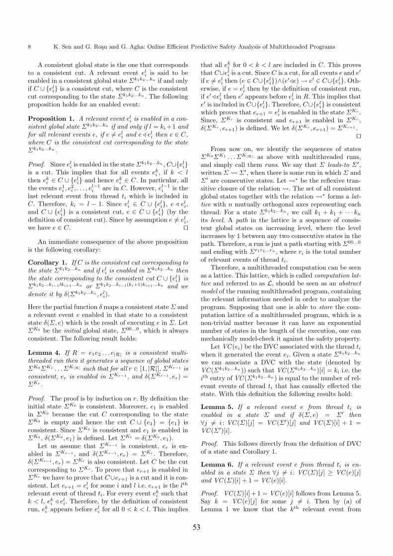
8 K. Sen and G. Rosu and G. Agha: Online Efficient Predictive Safety Analysis of Multithreaded Programs

A consistent global state is the one that correspondsto a consistent cut. A relevant event el

i is said to beenabled in a consistent global state Σk1k2...kn if and onlyif C ∪ el

i is a consistent cut, where C is the consistentcut corresponding to the state Σk1k2...kn . The followingproposition holds for an enabled event:

Proposition 1. A relevant event eli is enabled in a con-

sistent global state Σk1k2...kn if and only if l = ki +1 andfor all relevant events e, if e 6= el

i and e / eli then e ∈ C,

where C is the consistent cut corresponding to the stateΣk1k2...kn .

Proof. Since eli is enabled in the state Σk1k2...kn , C∪el

iis a cut. This implies that for all events ek

i , if k < lthen ek

i ∈ C ∪ eli and hence ek

i ∈ C. In particular, allthe events e1

i , e2i , . . . , e

l−1i are in C. However, el−1

i is thelast relevant event from thread ti which is included inC. Therefore, ki = l − 1. Since el

i ∈ C ∪ eli, e / el

i,and C ∪ el

i is a consistent cut, e ∈ C ∪ eli (by the

definition of consistent cut). Since by assumption e 6= eli,

we have e ∈ C. ut

An immediate consequence of the above propositionis the following corollary:

Corollary 1. If C is the consistent cut corresponding tothe state Σk1k2...kn and if el

i is enabled in Σk1k2...kn thenthe state corresponding to the consistent cut C ∪ el

i isΣk1k2...ki−1lki+1...kn or Σk1k2...ki−1(ki+1)ki+1...kn and wedenote it by δ(Σk1k2...kn , el

i).

Here the partial function δ maps a consistent state Σ anda relevant event e enabled in that state to a consistentstate δ(Σ, e) which is the result of executing e in Σ. LetΣK0 be the initial global state, Σ00...0, which is alwaysconsistent. The following result holds:

Lemma 4. If R = e1e2 . . . e|R| is a consistent multi-threaded run then it generates a sequence of global statesΣK0ΣK1 . . . ΣK|R| such that for all r ∈ [1, |R|], ΣKr−1 isconsistent, er is enabled in ΣKr−1 , and δ(ΣKr−1 , er) =ΣKr .

Proof. The proof is by induction on r. By definition theinitial state ΣK0 is consistent. Moreover, e1 is enabledin ΣK0 because the cut C corresponding to the stateΣK0 is empty and hence the cut C ∪ e1 = e1 isconsistent. Since ΣK0 is consistent and e1 is enabled inΣK0 , δ(ΣK0 , e1) is defined. Let ΣK1 = δ(ΣK0 , e1).

Let us assume that ΣKr−1 is consistent, er is en-abled in ΣKr−1 , and δ(ΣKr−1 , er) = ΣKr . Therefore,δ(ΣKr−1 , er) = ΣKr is also consistent. Let C be the cutcorresponding to ΣKr . To prove that er+1 is enabled inΣKr we have to prove that C∪er+1 is a cut and it is con-sistent. Let er+1 = el

i for some i and l i.e. er+1 is the lth

relevant event of thread ti. For every event eki such that

k < l, eki / el

i. Therefore, by the definition of consistentrun, ek

i appears before eli for all 0 < k < l. This implies

that all eki for 0 < k < l are included in C. This proves

that C∪eli is a cut. Since C is a cut, for all events e and e′

if e 6= eli then (e ∈ C∪el

i)∧(e′/e) → e′ ∈ C∪eli. Oth-

erwise, if e = eli then by the definition of consistent run,

if e′ /eli then e′ appears before el

i in R. This implies thate′ is included in C∪el

i. Therefore, C∪eli is consistent

which proves that er+1 = eli is enabled in the state ΣKr .

Since, ΣKr is consistent and er+1 is enabled in ΣKr ,δ(ΣKr , er+1) is defined. We let δ(ΣKr , er+1) = ΣKr+1 .

utFrom now on, we identify the sequences of states

ΣK0ΣK1 . . . ΣK|R| as above with multithreaded runs,and simply call them runs. We say that Σ leads-to Σ′,written Σ Ã Σ′, when there is some run in which Σ andΣ′ are consecutive states. Let Ã∗ be the reflexive tran-sitive closure of the relation Ã. The set of all consistentglobal states together with the relation Ã∗ forms a lat-tice with n mutually orthogonal axes representing eachthread. For a state Σk1k2...kn , we call k1 + k1 + · · · kn

its level. A path in the lattice is a sequence of consis-tent global states on increasing level, where the levelincreases by 1 between any two consecutive states in thepath. Therefore, a run is just a path starting with Σ00...0

and ending with Σr1r2...rn , where ri is the total numberof relevant events of thread ti.

Therefore, a multithreaded computation can be seenas a lattice. This lattice, which is called computation lat-tice and referred to as L, should be seen as an abstractmodel of the running multithreaded program, containingthe relevant information needed in order to analyze theprogram. Supposing that one is able to store the com-putation lattice of a multithreaded program, which is anon-trivial matter because it can have an exponentialnumber of states in the length of the execution, one canmechanically model-check it against the safety property.

Let VC (ei) be the DVC associated with the thread tiwhen it generated the event ei. Given a state Σk1k2...kn

we can associate a DVC with the state (denoted byVC (Σk1k2...kn)) such that VC (Σk1k2...kn)[i] = ki i.e. theith entry of VC (Σk1k2...kn) is equal to the number of rel-evant events of thread ti that has causally effected thestate. With this definition the following results hold:

Lemma 5. If a relevant event e from thread ti isenabled in a state Σ and if δ(Σ, e) = Σ′ then∀j 6= i : VC (Σ)[j] = VC (Σ′)[j] and VC (Σ)[i] + 1 =VC (Σ′)[i].

Proof. This follows directly from the definition of DVCof a state and Corollary 1.

Lemma 6. If a relevant event e from thread ti is en-abled in a state Σ then ∀j 6= i : VC (Σ)[j] ≥ VC (e)[j]and VC (Σ)[i] + 1 = VC (e)[i].

Proof. VC (Σ)[i]+1 = VC (e)[i] follows from Lemma 5.Say k = VC (e)[j] for some j 6= i. Then by (a) ofLemma 1 we know that the kth relevant event from

53

K. Sen and G. Rosu and G. Agha: Online Efficient Predictive Safety Analysis of Multithreaded Programs 9

thread tj causally precedes e i.e. ekj / e. Then by propo-

sition 1 ekj ∈ C, where C is the cut corresponding to

Σ. This implies that k ≤ VC (Σ)[j] which proves that∀j 6= i : VC (Σ)[j] ≥ VC (e)[j].

Lemma 7. If R = e1e2 . . . e|R| is a consistent mul-tithreaded run generating the sequence of global statesΣK0ΣK1 . . . ΣK|R| , then VC (ΣKi) can be recursively de-fined as follows:

VC (ΣK0)[j] = 0 for all j ∈ [1, n]VC (ΣKr )[j] = max (VC (ΣKr−1)[j],VC (er)[j])

for all j ∈ [1, n] and 0 < r ≤ |R|

Proof. ∀j ∈ [1, n] : VC (ΣK0)[j] = 0 holds by def-inition. Let er be from thread ti. By Lemma 4er is enabled in ΣKr−1 . Therefore, by Lemma 6,∀j 6= i : VC (ΣKr−1)[j] ≥ VC (er)[j]. This im-plies that ∀j 6= i : VC (ΣKr )[j] = VC (ΣKr−1)[j] =max (VC (ΣKr−1)[j],VC (er)[j]). Otherwise if j = i, byLemma 6, VC (ΣKr−1)[j] + 1 = VC (er)[j]. Therefore,VC (ΣKr )[j] = VC (ΣKr−1)[j] + 1 = VC (er)[j] =max (VC (ΣKr−1)[j],VC (er)[j]). This proves that∀j : VC (ΣKr )[j] = max (VC (ΣKr−1)[j],VC (er)[j]).

Corollary 2. If R = e1e2 . . . e|R| is a consistent mul-tithreaded run generating the sequence of global statesΣK0ΣK1 . . . ΣK|R| , then

VC (ΣKr )[i] = max (VC (e1)[i],VC (e2)[i], . . . ,VC (er)[i])for all i ∈ [1, n] and 0 < r ≤ |R|

Example 2. Figure 2 shows the causal partial order onrelevant events extracted by the observer from the mul-tithreaded execution in Example 1, together with thegenerated computation lattice. The actual execution,Σ00Σ01Σ11Σ12Σ22Σ23Σ33, is marked with solid edgesin the lattice. Besides its DVC, each global state in thelattice stores its values for the relevant variables, w andv. It can be readily seen on Fig. 2 that the LTL prop-erty F1 defined in Example 1 holds on the sample runof the system, and also that it is not in the language ofbad prefixes, F2. However, F1 is violated on some otherconsistent runs, such as Σ00Σ01Σ02Σ12Σ13Σ23Σ33. Onthis particular run ↑ p holds at Σ02; however, r doesnot hold at the next state Σ12. This makes the formulaF1 false at the state Σ13. The run can also be symboli-cally written as ppp, qp, q, rp, q, r. In theautomaton in Fig. 1, this corresponds to a possible se-quence of states 00123555. Hence, this string is acceptedby F2 as a bad prefix.

Therefore, by carefully analyzing the computationlattice extracted from a successful execution one caninfer safety violations in other possible consistent ex-ecutions. Such violations give informative feedback tousers, such as the lack of synchronization in the exam-ple above, and may be hard to find by just ordinarytesting. In what follows we propose effective techniques

to analyze the computation lattice. A first importantobservation is that one can generate it on-the-fly andanalyze it on a level-by-level basis, discarding the previ-ous levels. However, even if one considers only one level,that can still contain an exponential number of statesin the length of the current execution. A second impor-tant observation is that the states in the computationlattice are not all equiprobable in practice. By allow-ing a user configurable window of most likely states inthe lattice centered around the observed execution trace,the presented technique becomes quite scalable, requir-ing O(wm) space and O(twm) time, where w is the sizeof the window, m is the size of the bad prefix monitorof the safety property, and t is the size of the monitoredexecution trace.

4.2 Level By Level Analysis of the Computation Lattice

A naive observer of an execution trace of a multithreadedprogram would just check the observed execution traceagainst the monitor for the safety property, say Monlike in Definition 1, and would maintain at each mo-ment a set of states, say MonStates in M. When a newevent arrives, it would create the next state Σ and re-place MonStates by ρ(MonStates, Σ). If the bad stateb will ever be in MonStates then a property violationerror would be reported, meaning that the current exe-cution trace led to a bad prefix of the safety property.Here we assume that the events are received in the orderin which they are emitted, and also that the monitorworks over the global states of the multithreaded pro-grams. This assumption is essential for the observer todeduce the actual execution of the multithreaded pro-gram. The knowledge of the actual execution is used bythe observer to apply the causal cone heuristics as de-scribed later. The assumption is not necessary if we donot want to use causal cone heuristics. The work in [22]describes a technique for the level by level analysis ofthe computation lattice without the above assumption.

A smart observer, as said before, will analyze notonly the observed execution trace, but also all the otherconsistent runs of the multithreaded system, thus be-ing able to predict violations from successful executions.The observer receives the events from the running multi-threaded program in real-time and enqueues them in anevent queue Q. At the same time, it traverses the compu-tation lattice level by level and checks whether the badstate of the monitor can be hit by any of the runs upto the current level. We next provide the algorithm thatthe observer uses to construct the lattice level by levelfrom the sequence of events it receives from the runningprogram.

The observer maintains a list of global states (Cur-rLevel), that are present in the current level of the lat-tice. For each event e in the event queue, it tries to con-struct a new global state from the set of states in the cur-rent level and the event e. If the global state is created

54

10 K. Sen and G. Rosu and G. Agha: Online Efficient Predictive Safety Analysis of Multithreaded Programs

e6 :<v=70, T1 ,(3,3)>

e4 :<v=60, T1 ,(2,1)>

e3 :< w =27, T2 ,(0,2)>

e2 :<v=50, T1 ,(1,1)>

e1 :< w =24, T2 ,(0,1)>

e5 :< w =31, T2 ,(0,3)>

) 40 , 20 (

) ( 00

= =

=

v w

S L

) 70 , 31 (

, , ) ( 33

= =

=

v w

r q p S L

) 60 , 31 (

, , ) ( 23

= =

=

v w

r q p S L

) 50 , 31 (

, ) ( 13

= =

=

v w

q p S L

) 60 , 27 (

, ) ( 22

= =

=

v w

r p S L

) 40 , 31 (

, ) ( 03

= =

=

v w

q p S L

) 50 , 27 (

) ( 12

= =

=

v w

p S L

) 60 , 24 (

) ( 21

= =

=

v w

r S L

) 40 , 27 (

) ( 02

= =

=

v w

p S L

) 50 , 24 (

) ( 11

= =

=

v w

S L

) 40 , 24 (

) ( 01

= =

=

v w

S L

Fig. 2. Computation Lattice

successfully then it is added to the list of global states(NextLevel) for the next level of the lattice. The pro-cess continues until certain condition, levelComplete?()holds. At that time the observer says that the level iscomplete and starts constructing the next level by set-ting CurrLevel to NextLevel, NextLevel to empty set, andreallocating the space previously occupied by CurrLevel.Here the predicate levelComplete?() is crucial for gener-ating only those states in the level that are most likely tooccur in other executions, namely those in the window,or the causality cone, that is described in the next sub-section. The levelComplete? predicate is also discussedand defined in the next subsection. The pseudo-code forthe lattice traversal is given in Fig. 3.

Every global state Σ contains the value of all relevantshared variables in the program, a DVC VC (Σ) to repre-sent the latest events from each thread that resulted inthat global state. Here the predicate nextState? (Σ, e),checks if the event e is enabled in the state Σ, wherethreadId(e) returns the index of the thread that gener-ated the event e, VC (Σ) returns the DVC of the globalstate Σ, and VC(e) returns the DVC of the event e.The correctness of the function is given by Lemma 6. Itessentially says that event e can generate a consecutivestate for a state Σ, if and only if Σ “knows” everything eknows about the current evolution of the multithreadedsystem except for the event e itself. Note that e mayknow less than Σ knows with respect to the evolutionof other threads in the system, because Σ has globalinformation.

The function createState(Σ, e), which implementsthe function δ described in Corollary 1 creates a newglobal state Σ′, where Σ′ is a possible consistent globalstate that can result from Σ after the event e. Togetherwith each state Σ in the lattice, a set of states of the

while(not end of computation)Q ← enqueue(Q, NextEvent())while(constructLevel())

boolean constructLevel()for each e ∈ Q and Σ ∈ CurrLevel

if nextState?(Σ, e) NextLevel ← NextLevel ] createState(Σ, e)if levelComplete?(NextLevel , e, Q)

Q ← removeUselessEvents(CurrLevel , Q)CurrLevel ← NextLevelNextLevel ← ∅return true

return false

boolean nextState?(Σ, e)i ← threadId(e);if (∀j 6= i : VC (Σ)[j] ≥ VC (e)[j] and

VC (Σ)[i] + 1 = VC (e)[i]) return truereturn false

State createState(Σ, e)Σ′ ← new copy of Σj ← threadId(e); VC (Σ′)[j] ← VC (Σ)[j] + 1pgmState(Σ′)[var(e) ← value(e)]MonStates(Σ′) ← ρ(MonStates(Σ), Σ′)if b ∈ MonStates(Σ′)

output ′property may be violated′return Σ′

Fig. 3. Level-by-level traversal.

55

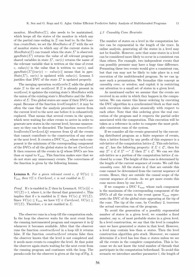
K. Sen and G. Rosu and G. Agha: Online Efficient Predictive Safety Analysis of Multithreaded Programs 11

monitor, MonStates(Σ), also needs to be maintained,which keeps all the states of the monitor in which anyof the partial runs ending in Σ can lead to. In the func-tion createState, we set the MonStates of Σ′ with the setof monitor states to which any of the current states inMonStates(Σ) can transit when the state Σ′ is observed.pgmState(Σ′) returns the value of all relevant programshared variables in state Σ′, var(e) returns the name ofthe relevant variable that is written at the time of evente, value(e) is the value that is written to var(e), andpgmState(Σ′)[var(e) ← value(e)] means that in pgm-State(Σ′), var(e) is updated with value(e). Lemma 5justifies that DVC of the state Σ′ is updated properly.

The merging operation nextLevel]Σ adds the globalstate Σ to the set nextLevel. If Σ is already present innextLevel, it updates the existing state’s MonStates withthe union of the existing state’s MonStates and the Mon-states of Σ. Two global states are same if their DVCs areequal. Because of the function levelComplete?, it may beoften the case that the analysis procedure moves fromthe current level to the next one before it is exhaustivelyexplored. That means that several events in the queue,which were waiting for other events to arrive in order togenerate new states in the current level, become unneces-sary so they can be discarded. The function removeUse-lessEvents(CurrLevel,Q) removes from Q all the eventsthat cannot contribute to the construction of any stateat the next level. It creates a DVC Vmin whose each com-ponent is the minimum of the corresponding componentof the DVCs of all the global states in the set CurrLevel.It then removes all the events in Q whose DVCs are lessthan or equal to Vmin . This function makes sure that wedo not store any unnecessary events. The correctness ofthe function is given by the following lemma.

Lemma 8. For a given relevant event e, if VC (e) ≤Vmin then ∀Σ ∈ CurrLevel , e is not enabled in Σ.

Proof. If e is enabled in Σ then by Lemma 6, VC (e)[i] =VC (Σ)+1, where ti is the thread that generated e. Thisimplies that if e is enabled in Σ then VC (e) 6≤ VC (Σ).Since VC (e) ≤ Vmin we have ∀Σ ∈ CurrLevel , VC (e) ≤VC (Σ). Therefore, e is not enabled in Σ.

The observer runs in a loop till the computation ends.In the loop the observer waits for the next event fromthe running instrumented program and enqueues it in Qwhenever it becomes available. After that the observerruns the function constructLevel in a loop till it returnsfalse. If the function constructLevel returns false thenthe observer knows that the level is not completed andit needs more events to complete the level. At that pointthe observer again starts waiting for the next event fromthe running program and continues with the loop. Thepseudo-code for the observer is given at the top of Fig. 3.

4.3 Causality Cone Heuristic

The number of states on a level in the computation lat-tice can be exponential in the length of the trace. Inonline analysis, generating all the states in a level maynot be feasible. However, note that some states in a levelcan be considered more likely to occur in a consistent runthan others. For example, two independent events thatcan possibly permute may have a huge time difference.Permuting these two events would give a consistent run,but that run may not be likely to take place in a realexecution of the multithreaded program. So we can ig-nore such a permutation. We formalize this concept ascausality cone, or window, and exploit it in restrictingour attention to a small set of states in a given level.

As mentioned earlier we assume that the events arereceived in an order in which they happen in the compu-tation. We can ensure this linear ordering by executingthe DVC algorithm in a synchronized block so that eachsuch execution takes place atomically with respect toeach other. Note that this ordering gives the real exe-cution of the program and it respects the partial orderassociated with the computation. This execution will betaken as a reference in order to compute the most prob-able consistent runs of the system.

If we consider all the events generated by the execut-ing distributed program as a finite sequence of events,then a lattice formed by any prefix of this sequence is asub-lattice of the computation lattice L. This sub-lattice,say L′, has the following property: if Σ ∈ L′, then forany Σ′ ∈ L if Σ′ Ã∗ Σ then Σ′ ∈ L′. We can see thissub-lattice as a portion of the computation lattice L en-closed by a cone. The height of this cone is determined bythe length of the current sequence of events. We call thiscausality cone. All the states in L that are outside thiscone cannot be determined from the current sequence ofevents. Hence, they are outside the causal scope of thecurrent sequence of events. As we get more events thiscone moves down by one level.

If we compute a DVC Vmax whose each componentis the maximum of the corresponding component of theDVCs of all the events in the event queue Vmax repre-sents the DVC of the global state appearing at the tip ofthe cone. The tip of the cone, by Corollary 2, traversesthe actual execution run of the program.

To avoid the generation of a possibly exponentialnumber of states in a given level, we consider a fixednumber, say w, of most probable states in a given level.In a level construction, we say that the level is completeonce we have generated w states in that level. However,a level may contain less than w states. Then the levelconstruction algorithm gets stuck. Moreover, we cannotdetermine if a level has less than w states unless we seeall the events in the complete computation. This is be-cause we do not know the total number of threads thatparticipate in the computation beforehand. To avoid thisscenario we introduce another parameter l, the length of

56

12 K. Sen and G. Rosu and G. Agha: Online Efficient Predictive Safety Analysis of Multithreaded Programs

w =3

< w =3

w

Fig. 4. Causality Cones

boolean levelComplete?(NextLevel, e, Q)if size(NextLevel) ≥ w then

return true;else if e is the last event in Q

and size(Q) == l thenreturn true;

else return false;

Fig. 5. levelComplete? predicate

the current event queue. We say that a level is completeif we have used all the events in the event queue for theconstruction of the states in the current level and thelength of the queue is l and we have not crossed thelimit w on the number of states. The pseudo-code forlevelComplete? is given in Fig. 5

Note, here l corresponds to the number of levels ofthe sub-lattice that can be constructed from the events inthe event queue Q. This is because, by Corollary 1, everyevent in the queue Q generates a state in the next levelfrom a state in the current level in which it is enabled.

Example 3. Figure 6 shows the portion of the computa-tion lattice constructed from the multithreaded execu-tion in Example 1 when the causality cone heuristics isapplied with parameters w = 2 and l = 3. The possibleconsistent run Σ00Σ01Σ02Σ03Σ13Σ23Σ33, shown on theleft side of the Figure 6, is pruned out by the heuristics.In this particular run the two independent events e2 ande5 that are permuted have long time difference in the ac-tual execution. Therefore, we can safely ignore this runamong all other possible consistent runs.

5 Implementation

We have implemented these new techniques, in version2.0 of the tool Java MultiPathExplorer (JMPaX), which

has been designed to monitor multithreaded Java pro-grams. The current implementation is written in Java.The tool has three main modules, the instrumentationmodule, the observer module and the monitor module.

The instrumentation program, named instrument,takes a specification file and a list of class files as com-mand line arguments. An example is

java instrument spec A.class B.class C.class

where the specification file spec contains a list ofnamed formulae written in a suitable logic. The programinstrument extracts the name of the relevant variablesfrom the specification and instruments the classes, pro-vided in the argument, as follows:

i) For each variable x of primitive type in eachclass it adds access and write DVCs, namely_access_dvc_x and _write_dvc_x, as new fields inthe class.

ii) It adds code to associate a DVC with every newlycreated thread;

iii) For each read and write access of a variable of prim-itive type in any class, it adds codes to update theDVCs according to the algorithm mentioned in Sec-tion 3.4;

iv) It adds code to call a method handleEvent of theobserver module at every write of a relevant vari-able.

The instrumentation module uses the BCEL [5] Java li-brary to modify Java class files. Currently, the instru-mentation module instruments every variable of prim-itive type in every class. This implies that, during theexecution of an instrumented program, the DVC algo-rithm is executed for every read and write of variablesof primitive type. This degrades the performance of theprogram considerably. We plan to improve the instru-mentation by using escape analysis [4], to detect the pos-sible shared variables through static analysis. This willreduce the number of instrumentation points and hencewill improve the performance.

The observer module, that takes two parametersw and l, generates the lattice level-by-level whenthe instrumented program is executed. Whenever thehandleEvent method is invoked, it enqueues the eventpassed as argument to the method handleEvent. Basedon the event queue and the current level of the lattice,it generates the next level. In the process, it invokes thenextStates method (corresponding to ρ in a monitor)of the monitor module.

The monitor module reads the specification file writ-ten either as an LTL formula or as a regular expressionand generates the non-deterministic automaton corre-sponding to the formula or the regular expression. Itprovides the method nextStates as an interface to theobserver module. The method raises an exception if atany point the set of states returned by nextStates con-tains the “bad” state of the automaton. The system be-

57

K. Sen and G. Rosu and G. Agha: Online Efficient Predictive Safety Analysis of Multithreaded Programs 13

e6 :<v=70, T1 ,(3,3)>

e4 :<v=60, T1 ,(2,1)>

e3 :< w =27, T2 ,(0,2)>

e2 :<v=50, T1 ,(1,1)>

e1 :< w =24, T2 ,(0,1)>

e5 :< w =31, T2 ,(0,3)>

) 40 , 20 (

) ( 00

= =

=

v w

S L

) 70 , 31 (

, , ) ( 33

= =

=

v w

r q p S L

) 60 , 31 (

, , ) ( 23

= =

=

v w

r q p S L

) 50 , 31 (

, ) ( 13

= =

=

v w

q p S L

) 60 , 27 (

, ) ( 22

= =

=

v w

r p S L

) 50 , 27 (

) ( 12

= =

=

v w

p S L

) 60 , 24 (

) ( 21

= =

=

v w

r S L

) 40 , 27 (

) ( 02

= =

=

v w

p S L

) 50 , 24 (

) ( 11

= =

=

v w

S L

) 40 , 24 (

) ( 01

= =

=

v w

S L

Fig. 6. Causality Cone Heuristics applied to Example 2

ing modular, the user can plug in his/her own monitormodule for his/her logic of choice.

Since in Java synchronized blocks cannot be inter-leaved, so corresponding events cannot be permuted,locks are considered as shared variables and a writeevent is generated whenever a lock is acquired or re-leased. This way, a causal dependency is generated be-tween any exit and any entry of a synchronized block,namely the expected happens-before relation. Java syn-chronization statements are handled exactly the sameway, that is, the shared variable associated to the syn-chronization object is written at the entrance and at theexit of the synchronized region. Condition synchroniza-tions (wait/notify) can be handled similarly, by gener-ating a write of a dummy shared variable by both thenotifying thread before notification and by the notifiedthread after notification.

Note that the above technique for handing synchro-nization constructs is conservative as it prevents us frompermuting two synchronized blocks even if the eventsin the two blocks are independent of each other. Futurework involves finding an extension of the DVC algorithmthat can allow such permutations. This will enable us toextract more interleavings from a computation.

6 Conclusion and Future Work

A formal runtime predictive analysis technique for mul-tithreaded systems has been presented in this paper, inwhich multiple threads communicating by shared vari-ables are automatically instrumented to send relevantevents, stamped by dynamic vector clocks, to an exter-

nal observer which extracts a causal partial order onthe global state, updates and thereby builds an abstractruntime model of the running multithreaded system. An-alyzing this model on a level-by-level basis, the observercan infer effectively, from a successful execution of the ob-served system, when safety properties can be violated byother executions. Attractive future work includes predic-tions of liveness violations and predictions of data-raceand deadlock conditions.

7 Acknowledgments

The work is supported in part by the Defense Ad-vanced Research Projects Agency (the DARPA IPTOTASK Program, contract number F30602-00-2-0586, theDARPA IXO NEST Program, contract number F33615-01-C-1907), the ONR Grant N00014-02-1-0715, the Mo-torola Grant MOTOROLA RPS #23 ANT, and the jointNSF/NASA grant CCR-0234524.

References

1. O. Babaoglu and K. Marzullo. Consistent global statesof distributed systems: Fundamental concepts and mech-anisms. In S. Mullender, editor, Distributed Systems,pages 55–96. Addison-Wesley, 1993.

2. H. Barringer, A. Goldberg, K. Havelund, and K. Sen.Rule-based runtime verification. In Proceedings of 5th In-ternational Conference on Verification, Model Checkingand Abstract Interpretation (VMCAI’04), volume 2937 ofLecture Notes in Computer Science, pages 44–57, Venice,Italy, January 2004. Springer-Verlag.

58

14 K. Sen and G. Rosu and G. Agha: Online Efficient Predictive Safety Analysis of Multithreaded Programs

3. H. W. Cain and M. H. Lipasti. Verifying sequential con-sistency using vector clocks. In Proceedings of the 14thannual ACM Symposium on Parallel Algorithms and Ar-chitectures, pages 153–154. ACM, 2002.

4. J. D. Choi, M. Gupta, M. J. Serrano, V. C. Sreedhar,and S. P. Midkiff. Escape analysis for java. In Proceed-ings of the 1999 ACM SIGPLAN Conference on Object-Oriented Programming Systems, Languages and Applica-tions (OOPSLA ’99), volume 34(10) of SIGPLAN No-tices, pages 1–19, Denver, Colorado, USA, November1999.

5. M. Dahm. Byte code engineering with the bcel api. Tech-nical Report B-17-98, Freie Universit at Berlin, Institutfur Informatik, April 2001.

6. J. Dick and A. Faivre. Automating the generation andsequencing of test cases from model-based specifications.In Proceedings of Formal Methods Europe (FME’93): In-dustrial Strength Formal Methods, volume 670 of LectureNotes in Computer Science, pages 268–284, 1993.

7. D. Drusinsky. Temporal rover. http://www.time-rover.com.

8. D. Drusinsky. The Temporal Rover and the ATG Rover.In SPIN Model Checking and Software Verification, vol-ume 1885 of Lecture Notes in Computer Science, pages323–330. Springer, 2000.

9. D. Drusinsky. Monitoring Temporal Rules Combinedwith Time Series. In Proc. of CAV’03: Computer AidedVerification, volume 2725 of Lecture Notes in ComputerScience, pages 114–118, Boulder, Colorado, USA, 2003.Springer-Verlag.

10. C. J. Fidge. Partial orders for parallel debugging. InProceedings of the 1988 ACM SIGPLAN and SIGOPSworkshop on Parallel and Distributed debugging, pages183–194. ACM, 1988.

11. E. L. Gunter, R. P. Kurshan, and D. Peled. PET: An in-teractive software testing tool. In Computer Aided Verifi-cation (CAV’00), volume 1885 of Lecture Notes in Com-puter Science, pages 552–556. Springer-Verlag, 2003.

12. K. Havelund and G. Rosu. Monitoring Java Programswith Java PathExplorer. In Proceedings of the 1st Work-shop on Runtime Verification (RV’01), volume 55 ofElectronic Notes in Theoretical Computer Science. El-sevier Science, 2001.

13. K. Havelund and G. Rosu. Synthesizing monitors forsafety properties. In Tools and Algorithms for Construc-tion and Analysis of Systems (TACAS’02), volume 2280of Lecture Notes in Computer Science, pages 342–356.Springer, 2002.

14. M. Kim, S. Kannan, I. Lee, and O. Sokolsky. Java-MaC:a Run-time Assurance Tool for Java. In Proceedings ofthe 1st Workshop on Runtime Verification (RV’01), vol-ume 55 of Electronic Notes in Theoretical Computer Sci-ence. Elsevier Science, 2001.

15. D. Lee and M. Yannakakis. Principles and methods oftesting finite state machines - A survey. In Proceedingsof the IEEE, volume 84, pages 1090–1126, 1996.

16. R. Lencevicius, A. Ran, and R. Yairi. Third eye -specification–based analysis of software execution traces.In International Workshop on Automated Program Anal-ysis, Testing and Verification (Workshop of ICSE 2000),pages 51–56, June 2000.

17. K. Marzullo and G. Neiger. Detection of global statepredicates. In Proceedings of the 5th International Work-shop on Distributed Algorithms (WADG’91), volume 579of Lecture Notes in Computer Science, pages 254–272.Springer-Verlag, 1991.

18. F. Mattern. Virtual time and global states of distributedsystems. In Parallel and Distributed Algorithms: proceed-ings of the International Workshop on Parallel and Dis-tributed Algorithms, pages 215–226. Elsevier, 1989.

19. A. Sen and V. K. .Garg. Partial order trace analyzer(pota) for distrubted programs. In Proceedings of the 3rdWorkshop on Runtime Verification (RV’03), ElectronicNotes in Theoretical Computer Science, 2003.

20. K. Sen and G. Rosu. Generating optimal monitors forextended regular expressions. In Proceedings of the 3rdWorkshop on Runtime Verification (RV’03), volume 89of ENTCS, pages 162–181. Elsevier Science, 2003.

21. K. Sen, G. Rosu, and G. Agha. Generating OptimalLinear Temporal Logic Monitors by Coinduction. InProceedings of 8th Asian Computing Science Conference(ASIAN’03), volume 2896 of Lecture Notes in ComputerScience, pages 260–275. Springer-Verlag, December 2003.

22. K. Sen, G. Rosu, and G. Agha. Runtime safety analysis ofmultithreaded programs. In Proceedings of 4th joint Eu-ropean Software Engineering Conference and ACM SIG-SOFT Symposium on the Foundations of Software Engi-neering (ESEC/FSE’03). ACM, 2003.

23. K. Sen, G. Rosu, and G. Agha. Online efficient predic-tive safety analysis of multithreaded programs. In Pro-ceedings of 10th International Conference on Tools andAlgorithms for the Construction and Analysis of Systems(TACAS’04), volume 2988 of Lecture Notes in ComputerScience, pages 123–138, Barcelona, Spain, March 2004.

24. O. Shtrichman and R. Goldring. The ‘logic-assurance’system - a tool for testing and controlling real-timesystems. In Proc. of the Eighth Israeli Conference oncomputer systems and sofware engineering (ICCSSE97),pages 47–55, June 1997.

25. L. J. Stockmeyer and A. R. Meyer. Word problems re-quiring exponential time (preliminary report). pages 1–9.ACM Press, 1973.

26. S. A. Vilkomir and J. P. Bowen. Formalization of soft-ware testing criteria using the Z notation. In Proceed-ings of COMPSAC 01: 25th IEEE Annual InternationalComputer Software and Applications Conference, pages351–356. IEEE Computer Society, Oct. 2001.

59

An Instrumentation Technique for Online Analysis of Multithreaded Programs

Grigore Rosu and Koushik SenDepartment of Computer Science,

University of Illinois at Urbana-Champaign, USAEmail: grosu,ksen@uiuc.edu

Abstract

Runtime verification of multithreaded systems, that is,the process of finding errors in multithreaded systems asthey execute, is the theme of this paper. The major goalof the work in this paper is to present an automatic codeinstrumentation technique, based onmultithreaded vectorclocks, for generating the causal partial order on relevantstate update events from a running multithreaded program.By means of several examples, it is shown how this tech-nique can be used in a formal testing environment, not onlyto detect, but especially topredict safety errorsin multi-threaded programs. The prediction process consists of rig-orously analyzing other potential executions that are con-sistent with the causal partial order: some of these can beerroneous despite the fact that the particular observed ex-ecution was successful. The proposed technique has beenimplemented as part of a Java program analysis tool, calledJava MultiPathExplorer and abbreviatedJMPAX. A byte-code instrumentation package is used, so the Java sourcecode of the tested programs is not necessary.

1. Introduction and Motivation

A major drawback of testing is its lack of coverage: if anerror is not exposed by a particular test case then that errorisnot detected. To ameliorate this problem, many techniqueshave been investigated in the literature to increase the cov-erage of testing, such as test-case generation methods forgenerating those test cases that can reveal potential errorswith high probability [8, 21, 30]. Based on experience withrelated techniques already implemented in JAVA PATHEX-PLORER (JPAX) [15, 14] and its sub-system EAGLE [4],we have proposed in [27, 28] an alternative approach, called“predictive runtime analysis”, which can be intuitively de-scribed as follows.

Suppose that a multithreaded program has a subtle safetyerror, such as a safety or a liveness temporal property vio-lation, or a deadlock or a data-race. Like in testing, one

executes the program on some carefully chosen input (testcase) and suppose that, unfortunately, the error is not re-vealed during that particular execution; such an executionis calledsuccessfulwith respect to that bug. If one regardsthe execution of a program as a flat, sequential trace ofevents or states, like NASA’s JPAX system [15, 14], Uni-versity of Pennsylvania’s JAVA -MAC [20], Bell Labs’ PET[13], or the commercial analysis systems Temporal Roverand DBRover [9, 10, 11], then there is not much left todo to find the error except to run another, hopefully bet-ter, test case. However, by observing the execution trace ina smarter way, namely as a causal dependency partial orderon state updates, one can predict errors that can potentiallyoccur in other possible runs of the multithreaded program.

The present work is an advance inruntime verification[16], a scalable complementary approach to the traditionalformal verification methods (such as theorem proving andmodel checking [6]). Our focus here is on multithreadedsystems with shared variables. More precisely, we presenta simple and effective algorithm that enables an externalobserver of an executing multithreaded program to detectand predict specification violations. The idea is to properlyinstrumentthe system before its execution, so that it willemit relevant events at runtime. No particular specificationformalism is adopted in this paper, but examples are givenusing a temporal logic that we are currently considering inJAVA MULTI PATHEXPLORER (JMPAX) [27, 28], a tool forsafety violation prediction in Java multithreaded programswhich supports the presented technique.

In multithreaded programs, threads communicate via aset of shared variables. Some variable updates can causallydepend on others. For example, if a thread writes a sharedvariablex and then another thread writesy due to a state-ment y = x + 1, then the update ofy causally dependsupon the update ofx. Only read-write, write-read and write-write causalities are considered, because multiple consec-utive reads of the same variable can be permuted withoutchanging the actual computation. A state is a map assigningvalues to variables, and a specification consists of propertieson these states. Some variables may be of no importance at

60

all for an external observer. For example, consider an ob-server which monitors the property “if(x > 0) then(y = 0)has been true in the past, and since then(y > z) was alwaysfalse”. All the other variables exceptx, y andz are irrele-vant for this observer (but they can clearly affect the causalpartial ordering). To minimize the number of messages sentto the observer, we consider a subset ofrelevant eventsandthe associatedrelevant causality.

We present an algorithm that, given an executing mul-tithreaded program, generates appropriate messages to besent to an external observer. The observer, in order to per-form its more elaborated system analysis, extracts the stateupdate information from such messages together with therelevant causality partial order among the updates. This par-tial order abstracts the behavior of the running program andis calledmultithreaded computation. By allowing an ob-server to analyze multithreaded computations rather thanjust flat sequences of events, one gets the benefit of notonly properly dealing with potential reordering of deliveredmessages (reporting global state accesses), but also ofpre-dicting errorsfrom analyzing successful executions, errorswhich can occur under a different thread scheduling and canbe hard, if not impossible, to find by just testing.

To be more precise, let us consider a real-life examplewhere a runtime analysis tool supporting the proposed tech-nique, such as JMPAX, would be able to predict a violationof a property from a single, successful execution of the pro-gram. However, like in the case of data-races, the chanceof detecting this safety violation by monitoring only the ac-tual run is very low. The example consists of a two threadedprogram to control the landing of an airplane. It has threevariableslanding, approved, andradio; their valuesare1 when theplane is landing, landing has been approved,andradio signal is live, respectively, and0 otherwise. Thesafety property to verify is “If the plane has started landing,then it is the case that landing has been approved and sincethe approval the radio signal has never been down.”

The code snippet for a naive implementation of this con-trol program is shown in Fig. 1. It uses some dummy func-tions, askLandingApproval and checkRadio, whichcan be implemented properly in a real scenario. The pro-gram has a serious problem that cannot be detected easilyfrom a single run. The problem is as follows. Suppose theplane has received approval for landing and just before itstarted landing the radio signal went off. In this situation,the plane must abort landing because the property was vio-lated. But this situation will very rarely arise in an execu-tion: namely, whenradio is set to 0 between the approvalof landing and the start of actual landing. So a tester or asimple observer will probably never expose this bug. How-ever, note that even if the radio goes offafter the landing hasstarted, a case which is quite likely to be considered duringtesting but in which the property isnot violated, JMPAX

int landing = 0, approved = 0, radio = 1;void thread1()

askLandingApproval();if(approved==1)

print("Landing approved");landing = 1;print("Landing started");

else print("Landing not approved");void askLandingApproval()

if(radio==0) approved = 0else approved = 1;

void thread2()while(radio)checkRadio();

void checkRadio()possibly change value of radio;

Figure 1. A buggy implementation of aflight controller.

will still be able to construct a possible run (counterexam-ple) in which radio goes off between landing and approval.In Section 4, among other examples, it is shown how JM-PAX is able to predict two safety violations from a singlesuccessful execution of the program. The user will be givenenough information (the entire counterexample execution)to understand the error and to correct it. In fact, this er-ror is an artifact of a bad programming style and cannot beeasily fixed - one needs to give a proper event-based imple-mentation. This example shows the power of the proposedruntime verification technique as compared to the existingones in JPAX and JAVA -MAC.

The main contribution of this paper is a detailed presen-tation of an instrumentation algorithm which plays a crucialrole in extracting the causal partial order from one flat exe-cution, and which is based on an appropriate notion of vec-tor clock inspired from [12, 24], calledmultithreaded vectorclock (MVC). An MVC V is an array associating a naturalnumberV [i] to each threadi in the multithreaded system,which represents the number of relevant events generatedby that thread since the beginning of the execution. AnMVC Vi is associated to each threadti, and two MVCs,V a

x

(access) andV wx (write) are associated to each shared vari-

ablex. When a threadti processes evente, which can bean internal event or a shared variable read/write, the codein Fig. 2 is executed. We prove thatA correctly imple-ments the relevant causal partial order, i.e., that for any twomessages〈e, i, V 〉 and 〈e′, j, V ′〉 sent byA, e and e′ arerelevant ande causally precedese′ iff V [i] ≤ V ′[i]. This al-gorithm can be implemented in several ways. In the case ofJava, we prefer to implement it as an appropriate instrumen-tation procedure of code or bytecode, to executeA when-ever a shared variable is accessed. Another implementationcould be to modify a JVM. Yet another one would be to en-

261

ALGORITHM AINPUT: evente generated by threadti

1. if e is relevant thenVi[i]← Vi[i] + 1

2. if e is a read of a shared variablex thenVi ← maxVi, V

wx

V ax ← maxV a

x , Vi

3. if e is a write of a shared variablex thenV w

x ← V ax ← Vi ← maxV a

x , Vi

4. if e is relevant thensend message〈e, i, Vi〉 to observer

Figure 2. The vector clock instrumen-tation algorithm.

force shared variable updates via library functions, whichexecuteA as well. All these can add significant delays tothe normal execution of programs. The work in this paperhas been partly presented at the workshopParallel and Dis-tributed Systems: Testing and Debugging (PADTAD’04)inApril 2004. A preliminary version has been published inthe PADTAD’04 proceedings [25].

Multithreaded systems are briefly introduced in Section2 and then the main algorithm is rigorouslyderivedfrom itsdesired properties in Section 3. Section 4 describes possibleuses of the algorithm, and Section 5 concludes the paper.

2. Multithreaded Systems

We consider multithreaded systems in which severalthreads communicate with each other via a set of sharedvariables. A crucial point is that some variable updates cancausally depend on others. We will present an instrumen-tation algorithm which, given an executing instrumentedmultithreaded program, generates appropriate messages tobe sent to an external observer. The observer, in order toperform its analysis, extracts the state update informationfrom such messages together with the causality partial or-der among the updates.

In this paper we only consider a fixed number of threads.However, the presented instrumentation technique can beeasily extended to systems consisting of a variable numberof threads, where these can be dynamically created and/ordestroyed [28].

2.1. Multithreaded Executions

Givenn threadst1, t2, ..., tn, amultithreaded executionis a sequence of eventse1e2 . . . er, each belonging to oneof then threads and having typeinternal, reador write ofa shared variable. We useek

i to represent thek-th eventgenerated by threadti since the start of its execution. Whenthe thread or position of an event is not important, we mayrefer to it generically, such ase, e′, etc. We may writee ∈ tiwhen evente is generated by threadti.

Let us fix an arbitrary but fixed multithreaded execution,sayM, and letS be the set of all shared variables. There isan immediate notion ofvariable access precedencefor eachshared variablex ∈ S: we say thate x-precedese′, writtene <x e′, if and only if e ande′ are variable access events(reads or writes) to the same variablex, ande “happensbefore”e′, that is,e occurs beforee′ inM. This “happens-before” relation can be easily realized in practice by keepinga counter for each shared variable, which is incremented ateach variable access.

The notion of precedence above is consistent with thesequential memory modelof multithreaded systems, whichis assumed from now on in this paper. In fact, we assumethat all shared memory accesses (reads or writes of sharedvariables inS) are atomic and instantaneous. this will al-low us to properly reason about causal dependencies be-tween events. For example, if a thread writesx then writesy followed by another thread writingy thenx, under a non-sequential memory model it would be possible that the firstwrite of y takes place before the second, while the first writeof x takes placeafter the second write ofx, leading to a cir-cular causal dependency between the two threads. So far wehave not considered non-sequential memory models in ourruntime verification efforts, which admittedly would revealadditional potential errors but would increase the complex-ity of runtime analysis. This may change in the future ifthe assumed sequential model will be found too restrictivein practical experiments. Recall that our purpose is to finderrors in multithreaded programs, not to prove systems cor-rect. The errors that we detect using the sequential modelare also errors in other memory models, so our approach iscurrently conservative.

2.2. Causality and Multithreaded Computations

Let E be the set of all the events occurring in the multi-threaded executionM and let≺ be the partial order relationonE defined as follows:

• eki ≺ el

i if k < l;

• e ≺ e′ if there isx ∈ S with e <x e′ and at least oneof e, e′ is a write;

362

• e ≺ e′′ if e ≺ e′ ande′ ≺ e′′.

The first item above states that the events of a threadi arecausally ordered by their corresponding occurrence time.The second item says that if two eventse ande′, of the samethread or not, access a shared variablex and one of them isa write, then the most recent one causally depends on theformer one. No causal constraint is imposed on read-readevents, so they are permutable. Finally, by closing it undertransitivity, the third item defines≺ as the smallest partialorder including the first two types of causal constraints. Wewrite e||e′ if e 6≺ e′ ande′ 6≺ e. The partial order≺ on Edefined above is called themultithreaded computationasso-ciated with the original multithreaded executionM.

As discussed in Section 3.1 in more depth, synchroniza-tion of threads can be handled at no additional effort by justgenerating appropriate read/write events when synchroniza-tion objects are acquired/released, so the simple notion ofmultithreaded computation as defined above is as generalas practically needed. A linearization (or a permutation) ofall the eventse1, e2, ...,er that is consistent with the multi-threaded computation, in the sense that the order of eventsin the permutation is consistent with≺, is called aconsis-tent multithreaded run, or simply, amultithreaded run. In-tuitively, a multithreaded run can be viewed as a possibleexecution of the same system under a different executionspeed of each individual thread.

A multithreaded computation can be thought of as themost general assumptionthat an observer of the multi-threaded execution can make about the system withoutknowing its semantics. Indeed, an external observer sim-ply cannot disregardthe order in which the same variable ismodified and used within the observed execution, becausethis order can be part of the intrinsic semantics of the multi-threaded program. However, multiple causally independentmodifications of different variables can be permuted, andthe particular order observed in the given execution is notcritical. By allowing an observer to analyzemultithreadedcomputations, rather than justmultithreaded executionslikeJPAX [15, 14], JAVA -MAC [20], and PET [13], one getsthe benefit of not only properly dealing with potential re-orderings of delivered messages (e.g., due to using multi-ple channels to reduce the monitoring overhead), but alsoof predicting errorsfrom analyzing successful executions,errors which can occur under a different thread scheduling.

2.3. Relevant Causality

Some variables inS may be of no importance for an ex-ternal observer. For example, consider an observer whosepurpose is to check the property “if(x > 0) then(y = 0)has been true in the past, and since then(y > z) was al-ways false”; formally, using the interval temporal logic no-tation notation in [18], this can be compactly written as

(x > 0) → [y = 0, y > z). All the other variables inSexceptx, y andz are essentially irrelevant for this observer.To minimize the number of messages, like in [23] whichsuggests a similar technique but for distributed systems inwhich reads and writes are not distinguished, we consider asubsetR ⊆ E of relevant eventsand define theR-relevantcausalityon E as the relation⊳ :=≺ ∩(R × R), so thate ⊳ e′ if and only if e, e′ ∈ R ande ≺ e′. It is importantto notice though that the other shared variables can also in-directly influence the relation⊳, because they can influencethe relation≺.

We next introduce multithreaded vector clocks (MVC),together with a technique that is proved to correctly imple-ment the relevant causality relation.

3. Multithreaded Vector Clock Algorithm

Inspired and stimulated by the elegance and naturalityof vector clocks [12, 24, 2] in implementing causal depen-dency in distributed systems, we next devise an algorithm toimplement the relevant causal dependency relation in mul-tithreaded systems. Since in multithreaded systems com-munication is realized by shared variables rather than mes-sage passing, to avoid any confusion we call the correspond-ing vector-clock data-structuresmultithreaded vector clocksand abbreviate them(MVC). The algorithm presented nexthas been mathematically derived from its desired proper-ties, after several unsuccessful attempts to design it on aless rigorous basis.

For each threadi, where1 ≤ i ≤ n, let us consider ann-dimensional vector of natural numbersVi. Intuitively, thenumberVi[j] represents the event number at threadtj thatthe threadti is “aware” of. Since communication in mul-tithreaded systems is done via shared variables, and sincereads and writes have different weights in our approach,we let V a

x andV wx be two additionaln-dimensional vec-

tors for each shared variablex; we call the formeraccessMVC and the latterwrite MVC. All MVCs are initialized to0. As usual, for twon-dimensional vectors,V ≤ V ′ if andonly if V [j] ≤ V ′[j] for all 1 ≤ j ≤ n, andV < V ′ ifand only if V ≤ V ′ and there is some1 ≤ j ≤ n suchthat V [j] < V ′[j]; also, maxV, V ′ is the vector withmaxV, V ′[j] = maxV [j], V ′[j] for each1 ≤ j ≤ n.

Our goal is to find a procedure that updates these MVCsand emits a minimal amount of events to an external ob-server, which can further efficiently extract the relevantcausal dependency relation. Formally, the requirements ofsuch a procedure, sayA, which works as an event filter, oran abstraction of the given multithreaded execution, mustinclude the following natural requirements.

Requirements for A. AfterA updates the MVCs as a con-sequence of the fact that threadti generates eventek

i duringthe multithreaded executionM, the following should hold:

463

(a) Vi[j] equals the number of relevant events oftj thatcausally precedeek

i ; if j = i and eki is relevant then

this number also includeseki ;

(b) V ax [j] equals the number of relevant events oftj that

causally precede the most recent event inM that ac-cessed (read or wrote)x; if i = j andek

i is a relevantread or write ofx event then this number also includeseki ;

(c) V wx [j] equals the number of relevant events oftj that

causally precede the most recent write event ofx; ifi = j andek

i is a relevant write ofx then this numberalso includesek

i .

Finally and most importantly,A should correctly implementthe relative causality (stated formally in Theorem 3).

We next show how such an algorithm can be derivedfrom its requirements above. In order to do it, let us firstintroduce some useful formal notation. For an eventek

i ofthreadti, let (ek

i ] be the indexed set(eki ]j1≤j≤n, where

(eki ]j is the setel

j | elj ∈ tj , el

j ∈ R, elj ≺ ek

i whenj 6= i and the setel

i | l ≤ k, eli ∈ R when j = i.

Intuitively, (eki ] contains all the events in the multithreaded

computation that causally precede or are equal toeki .

Lemma 1 With the notation above, for1 ≤ i, j ≤ n:

1. (el′

j ]j ⊆ (elj ]j if l′ ≤ l;

2. (el′

j ]j ∪ (elj ]j = (e

maxl′,lj ]j for anyl andl′;

3. (elj ]j ⊆ (ek

i ]j for anyelj ∈ (ek

i ]j ; and

4. (eki ]j = (el

j ]j for some appropriatel.

Proof: 1. is immediate, because for anyl′ ≤ l, any eventekj

at threadtj preceding or equal toel′

j , that is one withk ≤ l′,also precedesel

j .

2. follows by 1., because it is either the case thatl′ ≤ l, inwhich case(el′

j ]j ⊆ (elj ]j , or l ≤ l′, in which case(el

j ]j ⊆

(el′

j ]j . In either case2. holds trivially.

3. There are two cases to analyze. Ifi = j thenelj ∈ (ek

i ]j ifand only ifl ≤ k, so3. becomes a special instance of1.. Ifi 6= j then by the definition of(ek

i ]j it follows thatelj ≺ ek

i .

Sinceel′

j ≺ elj for all l′ < l and since≺ is transitive, it

follows readily that(elj ]j ⊆ (ek

i ]j .

4. Since(eki ]j is a finite set of totally ordered events, it has

a maximum element, sayelj . Hence,(ek

i ]j ⊆ (elj ]j . By 3.,

one also has(elj ]j ⊆ (ek

i ]j .

Thus, by4 above, one can uniquely and unambiguously en-code a set(ek

i ]j by just a number, namely the size of the cor-responding set(el

j ]j , i.e., the number of relevant events of

threadtj up to itsl-th event. This suggests that if the MVCVi maintained byA stores that number in itsj-th componentthen(a) in the list of requirements ofA would be fulfilled.

Before we formally show how reads and writes of sharedvariables affect the causal dependency relation, we need tointroduce some notation. First, since a write of a sharedvariable introduces a causal dependency between the writeevent and all the previous read or write events of the sameshared variable as well as all the events causally preced-ing those, we need a compact way to refer at any momentto all the read/write events of a shared variable, as wellas the events that causally precede them. Second, since aread event introduces a causal dependency to all the pre-vious write events of the same variable as well as all theevents causally preceding those, we need a notation to referto these events as well. Formally, ifek

i is an event in a mul-tithreaded computationM andx ∈ S is a shared variable,then let

(eki ]ax =

The thread-indexed set of all the relevantevents that are equal to or causally precedean evente accessingx, such thate occursbefore or it is equal toek

i inM,

(eki ]wx =

The thread-indexed set of all the relevantevents that are equal to or causally precedean evente writing x, such thate occursbefore or it is equal toek

i inM.

It is obvious that(eki ]wx ⊆ (ek

i ]ax. Some or all of thethread-indexed sets of events above may be empty. By con-vention, if an event, saye, does not exist inM, then we as-sume that the indexed sets(e], (e]ax, and(e]wx are all empty(rather than “undefined”). Note that ifA is implementedsuch thatV a

x andV wx store the corresponding numbers of

elements in the index sets of(eki ]ax and(ek

i ]wx immediatelyafter eventek

i is processed by threadti, respectively, then(b) and(c) in the list of requirements forA are also fulfilled.

Even though the sets of events(eki ], (ek

i ]ax and(eki ]wx have

mathematically clean definitions, they are based on totalknowledge of the multithreaded computationM. Unfor-tunately,M can be very large in practice, so the compu-tation of these sets may be inefficient if not done properly.Since our analysis algorithms areonline, we would like tocalculate these setsincrementally, as the observer receivesnew events from the instrumented program. A key factor indevising efficient update algorithms is to find equivalentre-cursivedefinitions of these sets, telling us how to calculatea new set of events from similar sets that have been alreadycalculated at previous event updates.

Let eki

Ri be the indexed set whosej components are

empty for allj 6= i and whosei-th component is either theone element setek

i wheneki ∈ R or the empty set other-

wise. With the notation introduced, the following important

564

recursive properties hold:

Lemma 2 Let eki be an event inM and letel

j be the eventpreceding1 it inM. If ek

i is

1. An internal event then

(eki ] = (ek−1

i ] ∪ eki

Ri ,

(eki ]ax = (el

j ]ax, for anyx ∈ S,

(eki ]wx = (el

j ]wx , for anyx ∈ S;

2. A read ofx event then

(eki ] = (ek−1

i ] ∪ eki

Ri ∪ (el

j ]wx ,

(eki ]ax = (ek

i ] ∪ (elj ]

ax,

(eki ]ay = (el

j ]ay, for anyy ∈ S with y 6= x,

(eki ]wz = (el

j ]wz , for anyz ∈ S;

3. A write ofx event then

(eki ] = (ek−1

i ] ∪ eki

Ri ∪ (el

j ]ax,

(eki ]ax = (ek

i ],(ek

i ]wx = (eki ],

(eki ]ay = (el

j ]ay, for anyy ∈ S with y 6= x,

(eki ]wy = (el

j ]wy , for anyy ∈ S with y 6= x.

Proof: 1. For the first equality, first recall thateki ∈ (ek

i ]if and only if ek

i is relevant. Therefore, it suffices to showthate ≺ ek

i if and only if e ≺ ek−1i for any relevant event

e ∈ R. Sinceeki is internal, it cannot be in relation<x

with any other event for any shared variablex ∈ S, so bythe definition of≺, the only possibilities are that eithere

is some eventek′

i of threadti with k′ < k, or otherwisethere is such an eventek′

i of threadti with k′ < k such thate ≺ ek′

i . Hence, it is either the case thate is ek−1i (soek−1

i isalso relevant) or otherwisee ≺ ek−1

i . In any of these cases,e ∈ (ek−1

i ]. The other two equalities are straightforwardconsequences of the definitions of(ek

i ]ax and(eki ]wx .

2. Like in the proof of1., eki ∈ (ek

i ] if and only if eki ∈ R,

so it suffices to show that for any relevant evente ∈ R,e ≺ ek

i if and only if e ∈ (ek−1i ] ∪ (el

j ]wx . Sinceek

i is a readof x ∈ S event, by the definition of≺ one of the followingmust hold:

• e = ek−1i . In this caseek−1

i is also relevant, soe ∈(ek−1

i ];

• e ≺ ek−1i . It is obvious in this case thate ∈ (ek−1

i ];

• e is a write ofx event ande <x eki . In this casee ∈

(elj ]

wx ;

• There is some write ofx evente′ such thate ≺ e′ ande′ <x ek

i . In this casee ∈ (elj ]

wx , too.

1If eki is the first event then we can assume thate

lj does not exist inM,

so by convention all the associated sets of events are empty

Therefore,e ∈ (ek−1i ] or e ∈ (el

j ]ax.

Let us now prove the second equality. By the definitionof (ek

i ]ax, one has thate ∈ (eki ]ax if and only if e is equal to

or causally precedes an event accessingx ∈ S that occursbefore or is equal toek

i in M. Sinceeki is a read ofx,

the above is equivalent to saying that either it is the casethat e is equal to or causally precedesek

i , or it is the casethate is equal to or causally precedes an event accessingx

that occursstrictly beforeeki inM. Formally, the above is

equivalent to saying that eithere ∈ (eki ] or e ∈ (el

j ]ax. If

y, z ∈ S andy 6= x then one can readily see (like in1.above) that(ek

i ]ay = (elj ]

ay and(ek

i ]az = (elj ]

az .

3. It suffices to show that for any relevant evente ∈ R,e ≺ ek

i if and only if e ∈ (ek−1i ]∪ (el

j ]ax. Sinceek

i is a writeof x ∈ S event, by the definition of≺ one of the followingmust hold:

• e = ek−1i . In this caseek−1

i ∈ R, soe ∈ (ek−1i ];

• e ≺ ek−1i . It is obvious in this case thate ∈ (ek−1

i ];

• e is an access ofx event (read or write) ande <x eki .

In this casee ∈ (elj ]

ax;

• There is some access ofx evente′ such thate ≺ e′ ande′ <x ek

i . In this casee ∈ (elj ]

ax, too.

Therefore,e ∈ (ek−1i ] or e ∈ (el

j ]ax.

For the second equality, note that, as for the second equa-tion in 2., one can readily see thate ∈ (ek

i ]ax if and only ife ∈ (ek

i ]∪(elj ]

ax. Butel

j ]ax ⊆ (ek

i ], so the above is equivalentto e ∈ (ek

i ]. A similar reasoning leads to(eki ]wx = (ek

i ]. Theequalities fory 6= x immediate, becauseek

i has no relationto accesses of other shared variables butx.

Since each component set of each of the indexed sets inthese recurrences has the form(ek

i ]i for appropriatei andk,and since each(ek

i ]i can be safely encoded by its size, onecan then safely encode each of the above indexed sets byan n-dimensional MVC; these MVCs are preciselyVi forall 1 ≤ i ≤ n andV a

x andV wx for all x ∈ S. It is a simple

exercise now to derive the following MVC update algorithmA (which was also given in Section 1):

ALGORITHM AINPUT: evente generated by threadti

1. if e is relevant thenVi[i]← Vi[i] + 1

2. if e is a read of a shared variablex thenVi ← maxVi, V

wx

V ax ← maxV a

x , Vi

3. if e is a write of a shared variablex thenV w

x ← V ax ← Vi ← maxV a

x , Vi

665

4. if e is relevant thensend message〈e, i, Vi〉 to observer

An interesting observation is that one can regard the prob-lem of recursively calculating(ek

i ] as a dynamic program-ming problem. As can often be done in dynamic program-ming problems, one can reuse space and derive the Algo-rithm A. Therefore,A satisfies all the stated requirements(a), (b) and(c), so they can be used as properties next inorder to show the correctness ofA:

Theorem 3 If 〈e, i, V 〉 and 〈e′, i′, V ′〉 are two messagessent byA, thene ⊳ e′ if and only ifV [i] ≤ V ′[i] (no typo:the secondi is not ani′) if and only ifV < V ′.

Proof: First, note thate ande′ are both relevant. The casei = i′ is trivial. Supposei 6= i′. Since, by requirement(a)for A, V [i] is the number of relevant events thatti gener-ated before and includinge and sinceV ′[i] is the number ofrelevant events ofti that causally precedee′, it is clear thatV [i] ≤ V ′[i] if and only if e ≺ e′. For the second part, ife ⊳ e′ thenV ≤ V ′ follows again by requirement(a), be-cause any event that causally precedese also precedese′.Since there are some indicesi andi′ such thate was gen-erated byti and e′ by ti′ , and sincee′ 6≺ e, by the firstpart of the theorem it follows thatV ′[i′] > V [i′]; there-fore, V < V ′. For the other implication, ifV < V ′ thenV [i] ≤ V ′[i], so the result follows by the first part of thetheorem.

3.1. Synchronization and Shared Variables

Thread communication in multithreaded systems wasconsidered so far to be accomplished by writing/readingshared variables, which were assumed to be knowna pri-ori. In the context of a language like Java, this assumptionworks only if the shared variables are declaredstatic; it isless intuitive when synchronization and dynamically sharedvariables are considered as well. Here we show that, underproper instrumentation, the basic algorithm presented in theprevious subsection also works in the context of synchro-nization statements and dynamically shared variables.

Since in Java synchronized blocks cannot be interleaved,so corresponding events cannot be permuted, locks are con-sidered as shared variables and a write event is generatedwhenever a lock is acquired or released. This way, a causaldependency is generated between any exit and any entry ofa synchronized block, namely the expected happens-beforerelation. Java synchronization statements are handled ex-actly the same way, that is, the shared variable associated tothe synchronization object is written at the entrance and atthe exit of the synchronized region. Condition synchroniza-tions (wait/notify) can be handled similarly, by generatinga write of a dummy shared variable by both the notifying

thread before notification and by the notified thread afternotification.

To handle variables that are dynamically shared, foreach variablex of primitive type in each class the instru-mentation program addsaccessandwrite MVCs, namely_access_mvc_x and_write_mvc_x, as new fields inthe class. Moreover, for each read and write access of avariable of primitive type in any class, it adds codes to up-date the MVCs according to the multithreaded vector clockalgorithm.

3.2. A Distributed Systems Interpretation

It is known that the various mechanisms for process in-teraction are essentially equivalent. This leads to the follow-ing natural question: could it be possible to derive the MVCalgorithm in this section from vector clock based algorithmsimplementing causality in distributed systems, such as theones in [2, 7]. The answer to this question is:almost.

Since writes and accesses of shared variables have differ-ent impacts on the causal dependency relation, the most nat-ural thing to do is to associate two processes to each sharedvariablex, one for accesses, sayxa and one for writes, sayxw. As shown in Fig. 3 right, a write ofx by threadi can beseen as sending a “request” message to writex to the “ac-cess process”xa, which further sends a “request” messageto the “write process”xw, which performs the action andthen sends an acknowledgment messages back toi. This isconsistent with step 3 of the algorithm in Fig. 2; to see this,note thatV w

x ≤ V ax at any time.

However, a read ofx is less obvious and does not seemto be interpretable by message passing updating the MVCsthe standard way. The problem here is that the MVC ofxa

needs to be updated with the MVC of the accessing threadi, the MVC of the accessing threadi needs to be updatedwith the current MVC ofxw in order to implant causal de-pendencies between previous writes ofx and the currentaccess, but the point here is that the MVC ofxw doesnot

a w a wi x x i x x

Figure 3. A distributed systems interpre-tation of reads (left) and writes (right).

766

have to be updated by reads ofx; this is what allows readsto be permutable by the observer. In terms of message pass-ing, like Fig. 3 shows, this says that the access processxa

sends ahiddenrequest message toxw (after receiving theread request fromi), whose only role is to “ask”xw send anacknowledgment message toi. By hidden message, markedwith dotted line in Fig. 3, we mean a message which isnot considered by the standard MVC update algorithm. Therole of the acknowledgment message is to ensure thati up-dates its MVC with the one of the write access processxw.

4. The Vector Clock Algorithm at Work

In this section we propose predictive runtime analysisframeworks in which the presented MVC algorithm canbe used, and describe by examples how we use it in JAVA

MULTI PATHEXPLORER (JMPAX) [27, 28, 19].The observer therefore receives messages of the form

〈e, i, V 〉 in any order, and, thanks to Theorem 3, can ex-tract the causal partial order⊳ on relevant events, which isits abstraction of the running program. Any permutationof the relevant events which is consistent with⊳ is calleda multithreaded run, or simply arun. Notice that each runcorresponds to some possible execution of the program un-der different execution speeds or scheduling of threads, andthat the observed sequence of events is just one such run.Since each relevant event contains global state update infor-mation, each run generates a sequence of global states. Ifone puts all these sequences together then one gets a lattice,called computation lattice. The reader is assumed famil-iar with techniques on how to extract a computation latticefrom a causal order given by means of vector clocks [24].Given a global property to analyze, the task of the observernow is to verify it against every path in the automatically ex-tracted computation lattice. JPAX and JAVA -MAC are ableto analyze only one path in the lattice. The power of ourtechnique consists of its ability to predict potential errors inother possible multithreaded runs.

Once a computation lattice containing all possible runs isextracted, one can start using standard techniques on debug-ging distributed systems, considering both state predicates[29, 7, 5] and more complex, such as temporal, properties[3, 5, 1, 4]. Also, the presented algorithm can be used asa front-end to partial order trace analyzers such as POTA[26]. Also, since the computation lattice acts like an abstractmodel of the running program, one can potentially run one’sfavorite model checker against any property of interest. Wethink, however, that one can do better than that if one takesadvantage of the specific runtime setting of the proposedapproach. The problem is that the computation lattice cangrow quite large, in which case storing it might become asignificant matter. Since events are received incrementallyfrom the instrumented program, one can buffer them at the

observer’s side and then build the lattice on a level-by-levelbasis in a top-down manner, as the events become available.The observer’s analysis process can also be performed in-crementally, so that parts of the lattice which become non-relevant for the property to check can be garbage-collectedwhile the analysis process continues.

If the property to be checked can be translated intoa finite state machine (FSM) or if one can synthesizeonline monitors for it, like we did for safety properties[28, 17, 18, 27], then one can analyze all the multithreadedrunsin parallel, as the computation lattice is built. The ideais to store the state of the FSM or of the synthesized monitortogether with each global state in the computation lattice.This way, in any global state, all the information neededabout the past can be stored via a set of states in the FSMor the monitor associated to the property to check, which istypically quite small in comparison to the computation lat-tice. Thus only one cut in the computation lattice is neededat any time, in particular one level, which significantly re-duces the space required by the proposed predictive analysisalgorithm.

Liveness properties apparently do not fit our runtime ver-ification setting. However, stimulated by recent encourag-ing results in [22], we believe that it is also worth exploringtechniques that canpredict violations of liveness properties.The idea here is to search for paths of the formuv in thecomputation lattice with the property that the shared vari-able global state of the multithreaded program reached byu is the same as the one reached byuv, and then to checkwhetheruvω satisfies the liveness property. The intuitionhere is that the system can potentially run into the infinitesequence of statesuvω (u followed by infinity many repe-titions of v), which may violate the liveness property. It isshown in [22] that the testuvω |= ϕ can be done in poly-nomial time and space in the sizes ofu, v andϕ, typicallylinear inuv, for almost any temporal logic.

4.1. Java MultiPathExplorer (JMPaX)

JMPAX [27, 28] is a runtime verification tool whichchecks a user defined specification against a running pro-gram. The specifications supported by JMPAX allow anytemporal logic formula, using an interval-based notationbuilt on state predicates, so our properties can refer to theentire history of states. Fig. 4 shows the architecture of JM-PAX. An instrumentation module parses the user specifica-tion, extracts the set of shared variables it refers to, i.e., therelevant variables, and theninstrumentsthe multithreadedprogram (which is assumed in bytecode form) as follows.Whenever a shared variable is accessed the MVC algorithmA in Section 3 is inserted; if the shared variable is relevantand the access is a write then the event is considered rel-evant. When the instrumented bytecode is executed, mes-

867

Specification

Java

Multithreaded

Program

Bytecode

Compile

Instrumentor

Instrumented

Bytecode

Translator

SpecificationImpl

LTL Monitor

Execute

Level 0

Level 5

Level 4

Level 3

Level 2

Level 1

Computation Lattice

Monitor

Execution Program Execution

JVM

Instrument

Event Stream

Instrumentation

Module Monitoring

Module

Figure 4. The Architecture of JMPAX.

sages〈e, i, V 〉 for relevant eventse are sent via a socket toan external observer.

The observer generates the computation lattice on alevel by level basis, checking the user defined specificationagainst all possible multithreaded runs in parallel. Note thatonly one of those runs was indeed executed by the instru-mented multithreaded program, and that the observer doesnot know it; the other runs arepotentialruns, they can occurin other executions of the program. Despite the exponentialnumber of potential runs, at most two consecutive levels inthe computation lattice need to be stored at any moment.[27, 28] gives more details on the particular implementa-tion of JMPAX. We next discuss two examples where JM-PAX can predict safety violations from successful runs; theprobability of detecting these bugs only by monitoring theobserved run, as JPAX and JAVA -MAC do, is very low.

Example 1. Let us consider the simple landing controllerin Fig.1, together with the property “If the plane has startedlanding, then it is the case that landing has been approvedand since then the radio signal has never been down.” Sup-pose that a successful execution is observed, in which theradio goes downafter the landing has started. After instru-mentation, this execution emits only three events to the ob-server in this order: a write ofapproved to 1, a write oflanding to 1, and a write ofradio to 0. The observercan now build the lattice in Fig.5, in which the states areencoded by triples<landing,approved,radio> and the

leftmost path corresponds to the observed execution. How-ever, the lattice contains two other runs both violating thesafety property. The rightmost one corresponds to the sit-

<1,1,1>

<1,1,0>

<0,0,1>

<0,1,1> <0,0,0>

<0,1,0>

Figure 5. Computation latticefor the program in Fig. 1.

uation when the radio goes down right between the testradio==0 and the actionapproved=1, and the inner onecorresponds to that in which the radio goes down betweenthe actionsapproved=1 andlanding=1. Both these erro-neous behaviors are insightful and very hard to find by test-ing. JMPAX is able to build the two counterexamples veryquickly, since there are only 6 states to analyze and threecorresponding runs, so it is able to give useful feedback.

Example 2. Let us now consider an artificial example in-tended to further clarify the prediction technique. Supposethat one wants to monitor the safety property “if(x > 0)then (y = 0) has been true in the past, and since then(y > z) was always false” against a multithreaded pro-gram in which initially x = −1, y = 0 and z = 0,with one thread containing the codex++; ...; y = x + 1and another containingz = x + 1; ...; x++. The dotsindicate code that is not relevant, i.e., that does not ac-cess the variablesx, y and z. This multithreaded pro-gram, after instrumentation, sends messages to JMPAX’sobserver whenever the relevant variablesx, y, z are up-dated. A possible execution of the program to be sent tothe observer can consist of the sequence of program states(−1, 0, 0), (0, 0, 0), (0, 0, 1), (1, 0, 1), (1, 1, 1), wherethe tuple(−1, 0, 0) denotes the state in whichx = −1, y =0, z = 0. Following the MVC algorithm, we can deducethat the observer will receive the multithreaded computationshown in Fig. 6, which generates the computation latticeshown in the same figure. Notice that the observed multi-threaded execution corresponds to just one particular multi-threaded run out of the three possible, namely the leftmostone. However, another possible run of the same computa-tion is the rightmost one, which violates the safety property.Systems like JPAX and JAVA -MAC that analyze only theobserved runs fail to detect this violation. JMPAX predictsthis bug from the original successful run.

968

S 0 ,0

x = -1, y = 0, z = 0

S 2 ,2

x = 1, y = 1, z = 1

S 2 ,1

x = 0, y = 1, z = 1

S 2 ,0

x = 0, y = 1, z = 0

S 1 ,1

x = 0, y = 0, z = 1

S 1 ,0

x = 0, y = 0, z = 0

e1 :<x=0, T1 ,(1,0)>

e4 :<x=1, T2 ,(1,2)>

e2 :< z =1, T2 ,(1,1)> e3 :< y =1, T1 ,(2,0)>

e2 :< z =1, T2 ,(1,1)> e3 :< y =1, T1 ,(2,0)>

e1 :<x=0, T1 ,(1,0)>

e2 :< z =1, T2 ,(1,1)>

e3 :< y =1, T1 ,(2,0)>

e4 :<x=1, T2 ,(1,2)>

T1

T2

S 1 ,2

x = 1, y = 0, z = 1

e4 :<x=1, T2 ,(1,2)>

e3 :< y =1, T1 ,(2,0)>

Figure 6. Computation lattice with three runs.

5. Conclusion

A simple and effective algorithm for extracting the relevantcausal dependency relation from a running multithreadedprogram was presented in this paper. This algorithm is sup-ported by JMPAX, a runtime verification tool able to detectand predict safety errors in multithreaded programs.

Acknowledgments. Many thanks to Gul Agha and Mark-Oliver Stehr for their inspiring suggestions and commentson several previous drafts of this work. The work is sup-ported in part by the Defense Advanced Research ProjectsAgency (the DARPA IPTO TASK Program, contract num-ber F30602-00-2-0586, the DARPA IXO NEST Pro-gram, contract number F33615-01-C-1907), the ONR GrantN00014-02-1-0715, the Motorola Grant MOTOROLA RPS#23 ANT, and the joint NSF/NASA grant CCR-0234524.

References

[1] M. Ahamad, M. Raynal, and G. Thia-Kime. An adaptiveprotocol for implementing causally consistent distributedservices. InProceedings of International Conference onDistributed Computing (ICDCS’98), pages 86–93, 1998.

[2] O. Babaoglu and K. Marzullo. Consistent global statesof distributed systems: Fundamental concepts and mecha-

nisms. In S. Mullender, editor,Distributed Systems, pages55–96. Addison-Wesley, 1993.

[3] O. Babaoglu and M. Raynal. Specification and verificationof dynamic properties in distributed computations.Journalof Parallel and Distr. Computing, 28(2):173–185, 1995.

[4] H. Barringer, A. Goldberg, K. Havelund, and K. Sen. Rule-Based Runtime Verification. InProceedings Verification,Model Checking and Abstract Interpretation (VMCAI 04),volume 2937 ofLNCS, pages 44–57, Jan. 2004.

[5] C. M. Chase and V. K. Garg. Detection of global predicates:Techniques and their limitations.Distributed Computing,11(4):191–201, 1998.

[6] E. M. Clarke and J. M. Wing. Formal methods: state ofthe art and future directions.ACM Computing Surveys,28(4):626–643, Dec. 1996.

[7] R. Cooper and K. Marzullo. Consistent detection of globalpredicates.ACM SIGPLAN Notices, 26(12):167–174, 1991.Proceedings of the ACM/ONR Workshop on Parallel andDistributed Debugging.

[8] J. Dick and A. Faivre. Automating the generation and se-quencing of test cases from model-based specifications. InProceedings of Formal Methods Europe (FME’93): Indus-trial Strength Formal Methods, volume 670 ofLNCS, pages268–284, 1993.

[9] D. Drusinsky. Temporal rover. http://www.time-rover.com.[10] D. Drusinsky. The Temporal Rover and the ATG Rover.

In Proc. of SPIN’00: SPIN Model Checking and SoftwareVerification, volume 1885 ofLecture Notes in ComputerScience, pages 323–330, Stanford, California, USA, 2000.Springer.

[11] D. Drusinsky. Monitoring Temporal Rules Combined withTime Series. InProc. of CAV’03: Computer Aided Verifi-cation, volume 2725 ofLecture Notes in Computer Science,pages 114–118, Boulder, Colorado, USA, 2003. Springer-Verlag.

[12] C. J. Fidge. Partial orders for parallel debugging. InPro-ceedings of the 1988 ACM SIGPLAN/SIGOPS workshop onParallel and Distr. Debugging, pages 183–194. ACM, 1988.

[13] E. L. Gunter, R. P. Kurshan, and D. Peled. PET: An inter-active software testing tool. InComputer Aided Verification(CAV’00), volume 1885 ofLNCS, pages 552–556. Springer-Verlag, 2003.

[14] K. Havelund and G. Rosu. Monitoring Java Programs withJava PathExplorer. InProceedings of the 1st Workshop onRuntime Verification (RV’01), volume 55 ofENTCS. Else-vier, 2001.

[15] K. Havelund and G. Rosu. Monitoring Programs usingRewriting. In Proceedings Automated Software Engineer-ing (ASE’01), pages 135–143. IEEE, 2001.

[16] K. Havelund and G. Rosu.Runtime Verification 2001, 2002,volume 55, 70(4) ofENTCS. Elsevier, 2001, 2002. Proceed-ings of aComputer Aided Verification (CAV’01, CAV’02)workshop.

[17] K. Havelund and G. Rosu. Efficient monitoring of safetyproperties.Software Tools and Tech. Transfer, to appear.

[18] K. Havelund and G. Rosu. Synthesizing monitors for safetyproperties. InTools and Algorithms for Construction andAnalysis of Systems (TACAS’02), volume 2280 ofLNCS,pages 342–356. Springer, 2002.

1069

[19] Java MultiPathExplorer.http://fsl.cs.uiuc.edu/jmpax.[20] M. Kim, S. Kannan, I. Lee, and O. Sokolsky. Java-MaC: a

Run-time Assurance Tool for Java. InProceedings of Run-time Verification (RV’01), volume 55 ofENTCS. ElsevierScience, 2001.

[21] D. Lee and M. Yannakakis. Principles and methods of test-ing finite state machines - A survey. InProceedings of theIEEE, volume 84, pages 1090–1126, 1996.

[22] N. Markey and P. Schnoebelen. Model checking a path (pre-liminary report). InProceedings of the 14th InternationalConference on Concurrency Theory (CONCUR’2003), vol-ume 2761 ofLNCS, pages 248–262. Springer, 2003.

[23] K. Marzullo and G. Neiger. Detection of global state predi-cates. InProceedings of the 5th International Workshop onDistributed Algorithms (WADG’91), volume 579 ofLNCS,pages 254–272. Springer, 1991.

[24] F. Mattern. Virtual time and global states of distributed sys-tems. InParallel and Distributed Algorithms: proceedingsof the International Workshop on Parallel and DistributedAlgorithms, pages 215–226. Elsevier, 1989.

[25] G. Rosu and K. Sen. An instrumentation technique for on-line analysis of multithreaded programs. InPADTAD work-shop at IPDPS. IEEE Computer Society, 2003.

[26] A. Sen and V. K. .Garg. Partial order trace analyzer (pota)for distrubted programs. InProceedings of Workshop onRuntime Verification (RV’03), ENTCS, 2003.

[27] K. Sen, G. Rosu, and G. Agha. Runtime safety analysis ofmultithreaded programs. InEuropean Software EngineeringConference and ACM SIGSOFT Symposium on the Founda-tions of Software Engineering (ESEC/FSE’03). ACM, 2003.

[28] K. Sen, G. Rosu, and G. Agha. Online efficient predictivesafety analysis of multithreaded programs. In10th Inter-national Conference on Tools and Algorithms for the Con-struction and Analysis of Systems (TACAS’04), volume 2988of LNCS, pages 123–138, Bercelona, Spain, Mar. 2004.Springer.

[29] S. D. Stoller. Detecting global predicates in distributedsystems with clocks. InProceedings of the 11th Inter-national Workshop on Distributed Algorithms (WDAG’97),pages 185–199, 1997.

[30] S. A. Vilkomir and J. P. Bowen. Formalization of soft-ware testing criteria using the Z notation. InProceedingsof COMPSAC 01: 25th IEEE Annual International Com-puter Software and Applications Conference, pages 351–356. IEEE Computer Society, Oct. 2001.

1170

ON PARALLEL vs. SEQUENTIAL THRESHOLD CELLULAR AUTOMATA

PREDRAG TOSIC∗ and GUL AGHAOpen Systems Laboratory (http://osl.cs.uiuc.edu), Department of Computer Science,

University of Illinois at Urbana-Champaign, 201 N. Goodwin, Urbana, IL 61801, USAp-tosic, agha@cs.uiuc.edu

ABSTRACTCellular automata (CA) are an abstract model of fine-grain parallelism,

as the node update operations are rather simple, and therefore comparableto the basic operations of the computer hardware. In a classical CA, all thenodes execute their operations in parallel and in perfect synchrony. Weconsider herewith the sequential version of CA, called SCA, and comparethese SCA with the classical, parallel CA. In particular, we show thatthere are 1-D CA with very simple node state update rules that cannot besimulated by any comparable SCA, irrespective of the node update order-ing. Consequently, the fine granularity of the basic CA operations and,therefore, the fine-grain parallelism of the classical, synchronous CA,insofar as the “interleaving semantics” is concerned, is not fine enough.We also share some thoughts on how to extend the results herein, and, inparticular, we try to motivate the study of genuinely asynchronous cellularautomata.

Keywords: cellular automata, linear threshold automata, dynamical sys-tems, concurrency, sequential interleaving semantics

1. Introduction and Motivation

Cellular automata (CA) were originally introduced as an abstract mathematical model that cancapture the behavior of biological systems capable of self-reproduction [19]. Subsequently, CA havebeen extensively studied in a great variety of application domains, mostly in the context of complexphysical or biological systems and their dynamics (e.g., [11, 26, 27, 28, 29]). However, CA can alsobe viewed as an abstraction of massively parallel computers (e.g, [8]). Herein, we study a particularsimple yet nontrivial class of CA from the parallel and distributed computing perspectives. Inparticular, we pose - and partially answer - some fundamental questions regarding the nature of theCA parallelism, i.e., the perfect synchrony of the classical CA computation.

It is well known that CA are an abstract architecture model of fine-grain parallelism, in thatthe elementary operations executed at each node are rather simple and hence comparable to thebasic operations performed by the computer hardware. In a classical (parallel) CA, whether finite orinfinite, all the nodes execute their operations in parallel and in perfect synchrony, that is, logicallysimultaneously: in general, the state of a node xi at time step t + 1 is some simple function of thestates of the node xi and a set of its pre-specified neighbors at time t.

We consider herewith the sequential version of CA, that we shall abridge to SCA in the sequel,and compare these SCA with the perfectly synchronous parallel (or concurrent) CA. In particular,we will show that there are 1-D CA with very simple state update rules that cannot be simulated byany comparable SCA, irrespective of the node update ordering. While the result would be trivial ifone considers a single (S)CA computation, we argue that the result is nontrivial and important whenapplied to all possible inputs (starting configurations) and, moreover, to the entire classes of CA andSCA. Hence, the granularity of the basic CA operations, insofar as the (im)possibility of simulating

∗Contact author. Work phone: 217-244-1976. Fax: 217-333-9386.

171

their concurrent computation via appropriate sequential interleavings of these basic operations, turnsout not to be quite fine enough. We also share some thoughts on how to extend the resultspresented herein, and, in particular, we try to motivate the study of genuinely asynchronous cellularautomata, where the asynchrony applies not only to the local computations at individual nodes, butalso to the communication among different nodes via the “shared variables” stored as the respectivenodes’ states.

An example of asynchrony in the local node updates (i.e., asynchronous computation at different“processors”) is when, for instance, the individual nodes update one at a time, according to somerandom order. This is a kind of asynchrony found in the literature, e.g., in [14, 15]. It is importantto understand, however, that even in case of what is referred to as asynchronous cellular automata(ACA) in the literature, the term asynchrony there applies to local updates (i.e., computations)only, but not to communication, since a tacit assumption of the globally accessible global clockstill holds. We prefer to refer to this kind of (weakly asynchronous) (A)CA as sequential cellularautomata, and, in this work, consistently keep the term asynchronous cellular automata for thoseCA that do not have a global clock (see Section 4).

Before dwelling into the issue of concurrency vs. arbitrary sequential interleavings applied to thethreshold cellular automata, we first clarify the terminology, and then introduce the relevant conceptsthrough a simple programming exercise in Subsection 1.1.

Throughout, we use the terms parallel and concurrent as synonyms. Many programming lan-guages experts would strongly disagree with this convention. However, a complete agreement in thecomputer science community on what exactly concurrency means, and how it relates to parallelism,is lacking. According to Chapter §12 of [22], “concurrency in the programming language andparallelism in the computer hardware are independent concepts. [...] We can have concurrency in aprogramming language without parallel hardware, and we can have parallel execution without con-currency in the language. In short, concurrency refers to the potential for parallelism” (italics ours).Clearly, our convention herein does not conform to the notions of concurrency and parallelism asdefined in [22]. In contrast, [20] uses the term concurrent “to describe computations where the si-multaneously executing processes can interact with one another”, and parallel for “[...] computationswhere behavior of each process is unaffected by the behavior of the others”. [20] also acknowledgesthat many authors do not discriminate between “parallel” and “concurrent”. We shall follow thislatter convention throughout and, moreover, by a parallel (concurrent) computation we shall meanactions of several processing units that are carried out logically (if not necessarily physically) simul-taneously. That is, when referring to parallel (or, equivalently, concurrent) computation, we shallalways assume a perfect synchrony.

1.1. Capturing Concurrency by Sequential Interleavings

While our own brains are massively parallel computing devices, we seem to (consciously) thinkand approach problem-solving rather sequentially. In particular, when designing a parallel algorithmor writing a computer program that is inherently parallel, we still prefer to be able to understandsuch an algorithm or program at the level of sequential operations or executions. It is not surprising,therefore, that a great deal of research effort has been devoted to interpreting parallel computationin the more familiar, sequential terms. One of the most important contributions in that respect isthe (nondeterministic) sequential interleaving semantics of concurrency (see, e.g., [7, 9, 13, 17, 18]).

When interpreting concurrency via interleaving semantics, a natural question arises: Given aparallel computing model, can its parallel execution always be captured by such sequential nondeter-minism, so that any given parallel computation can be faithfully reproduced via an appropriate choiceof a sequential interleaving of the operations involved? For most theoreticians of parallel computinga,

aThat is, for all “believers” in the interleaving semantics of concurrency - as contrasted with, e.g., proponents of

272

the answer is apparently “Yes” - provided that we simulate concurrent execution via sequential in-terleavings at a sufficiently high level of granularity of the basic computational operations. However,given a parallel computation in the form of a set of concurrently executing processes, how do we tell ifthe particular level of granularity is fine enough, i.e., whether the operations at that granularity levelcan truly be rendered atomic for the purposes of capturing concurrency via sequential interleavings?

We shall illustrate the concept of sequential interleaving semantics of concurrency with a simpleexample. Let’s consider the following trivia question from a sophomore parallel programming class:Find a simple example of two instructions such that, when executed in parallel, they give a result notobtainable from any corresponding sequential execution sequence?

A possible answer: Assume x = 0 initially and consider the following two programs

x ← x + 1; x ← x + 1vs.

x ← x + 1 || x ← x + 1

where “||” stands for the parallel, and “;” for the sequential composition of instructions or programs,respectively. Sequentially, one always gets the same answer: x = 2. In parallel (when the twoassignment operations are executed synchronously), however, one gets x = 1. It appears, therefore,that no sequential ordering of operations can reproduce parallel computation - at least not at thegranularity level of high-level instructions as above.

The whole “mystery” can be readily resolved if we look at the possible sequential executions ofthe corresponding machine instructions:

LOAD x, ∗m LOAD x, ∗mADD x, #1 ADD x, #1STORE x, ∗m STORE x, ∗mThere certainly exist choices of sequential interleavings of the six machine instructions above that

lead to “parallel” behavior (i.e., the one where, after the code is executed, x = 1). Thus, byrefining granularity from the high-level language instructions down to the machine instructions, wecan certainly preserve the interleaving “semantics” of concurrency.

As a side, we remark that it turns out that the example above does not require finer granularityquite yet, if we allow that some instructions be treated as no-ops. Indeed, if we informally defineΦ(P ) to be the set of possible behaviors of program P, then the example above only shows that, forS1 = S2 = (x ← x + 1),

Φ(S1||S2) * Φ(S1; S2) ∪ Φ(S2; S1) (1)

However, it turns out that, in this particular example, it indeed is the case that

Φ(S1||S2) ⊆ Φ(S1; S2) ∪ Φ(S2; S1) ∪ Φ(S1) ∪ Φ(S2) (2)

and no finer granularity is necessary to model Φ(S1||S2), assuming that, in some of the sequentialinterleavings, we allow certain instructions not to be executed at all.

However, one can construct more elaborate examples where the property (2) does not hold.The only way to capture the program behavior of parallel compositions of the form Φ(P1||P2) viasequential interleavings in such cases would then be to find a finer level of granularity, i.e., to reconsiderat what level can operations be considered atomic, so that the union of all possible sequentialinterleavings of such basic operations (including the interleavings that allow “no-ops” for some ofthe instructions) is guaranteed to capture the concurrent behavior, i.e., so that (2) holds. Thatis, sometimes refining the granularity of operations so that sequential interleavings can capturesynchronous parallel behavior, becomes a necessity.

true concurrency, an alternative model not discussed herewith.

373

We address herein the (in)adequacy of the sequential interleavings semantics when applied to CAwhere the individual node updatesb are considered to be elementary operations. In particular, weshow that the perfect synchrony of the classical CA’s node updates causes the interleaving semantics,as captured by the SCA and NICA sequential CA models (Section 2), to fail rather dramaticallyeven in the context of the simplest (nonlinear) CA node update rules.

2. Cellular Automata and Types of Their Configurations

We introduce CA by first considering (deterministic) Finite State Machines (FSMs) such asDeterministic Finite Automata (DFA). An FSM has finitely many states, and is capable of readingthe input signals coming from the outside. The machine is initially in some starting state; uponreading each input signal, the machine changes its state according to a pre-defined and fixed rule.In particular, the entire memory of the system is contained in what “current state” the machine isin, and nothing else about the previously processed inputs is remembered. Hence, the probabilisticgeneralization of deterministic FSMs leads to (discrete) Markov chains. It is important to noticethat there is no way for a FSM to overwrite, or in any other way affect, the input data stream. Thusindividual FSMs are computational devices of rather limited power.

Now let us consider many such FSMs, all identical to one another, that are lined up togetherin some regular fashion, e.g., on a straight line or a regular 2-D grid, so that each single “node”in the grid is connected to its immediate neighbors. Let’s also eliminate any external sources ofinput streams to the individual machines at the nodes, and let the current values of any given node’sneighbors be that node’s only “input data”. If we then specify a finite set of the possible values heldin each node, and we also identify this set of values with the set of each node’s internal states, wearrive at an informal definition of a classical cellular automaton. To summarize, a CA is a finiteor infinite regular grid in one-, two- or higher-dimensional space, where each node in the grid is aFSM, and where each such node’s input data at each time step are the corresponding internal statesof the node’s neighbors. Moreover, in the most important special case - the Boolean case, this FSMis particularly simple, i.e., it has only two possible internal states, labeled 0 and 1. All the nodesof a classical CA execute the FSM computation in unison, i.e., (logically) simultaneously. Wenote that infinite CA are capable of universal (Turing) computation. Moreover, the general class ofinfinite CA, once arbitrary starting configurations are allowed, are actually strictly more powerfulthan the classical Turing machines (for more, see, e.g., [8]).

We follow [8] and formally define classical (that is, synchronous and concurrent) CA in two steps:we first define the notion of a cellular space, and, subsequently, we define a cellular automaton overan appropriate cellular space.

Definition 1 A Cellular Space, Γ, is an ordered pair (G,Q), where

• G is a regular undirected Cayley graph that may be finite or infinite, with each node labeledwith a distinct integer; and

• Q is a finite set of states that has at least two elements, one of which being the special quiescentstate, denoted by 0.

We denote the set of integer labels of the nodes (vertices) in Γ by L. That is, L may be equal to,or be a proper subset of, the set of all integers.

bIt is tacitly assumed here that the complete node update operation includes, in addition to computing the localupdate function on appropriate inputs, also the necessary reads of the neighbors’ values preceding the local rulecomputation, as well as the writes of one’s new value following the local computation. These points will become clearonce the necessary definitions and terminology are introduced in Section 2; see also discussion in Sections 4 and 5.

474

Definition 2 A Cellular Automaton A is an ordered triple (Γ, N, M), where

• Γ is a cellular space;• N is a fundamental neighborhood; and• M is a finite state machine such that the input alphabet of M is Q|N |, and the local transition

function (update rule) for each node is of the form δ : Q|N |+1 → Q for CA with memory, andδ : Q|N | → Q for memoryless CA.

The fundamental neighborhood N specifies what near-by nodes provide inputs to the update ruleof a given node. In the classical CA, Γ is a regular graph that locally “looks the same everywhere”;in particular, the local neighborhood N is the same for each node in Γ.

The local transition rule δ specifies how each node updates its state (that is, value), based onits current state (value), and the current states of its neighbors in N . By composing together theapplication of the local transition rule to each of the CA’s nodes, we obtain the global map on theset of (global) configurations of a cellular automaton.

We observe that there is plenty of parallelism in the CA “hardware”, assuming, of course, asufficiently large number of nodesc. Actually, classical CA defined over infinite cellular spaces provideunbounded parallelism where, in particular, an infinite amount of information processing is carriedout in a finite time (even in a single parallel step). In particular, the notion of independence betweenparallelism and concurrency as defined in [22] seems inappropriate to apply to CA: without theparallel “hardware”, that is, multiple interconnected nodes, a CA is not capable of any concurrentcomputation. Indeed, a single-node CA is just a “fixed” deterministic FSM - an entirely sequentialcomputing model.

Insofar as the CA “computer architecture” is concerned, one important characteristic is thatthe memory and the processors are not truly distinguishable, in stark contrast to Turing machines,(P)RAMs, and other standard abstract models of digital computers. Namely, each node of a cellularautomaton is both a processing unit and a memory storage unit; see, e.g., the detailed discussionin [24]. In particular, the only “memory content” of a CA is a tuple of the (current) states of allits nodes. Moreover, as a node can “read” (but not “write”) the states or “values” of its neighbors,we can view the architecture of classical CA as a very simplistic, special case of distributed sharedmemory parallel model, where every “processor” (that is, each node) “owns” one cell (typically, onebit) of its “local memory”, physically separated from other similar local “memories” - yet this localmemory is directly accessible (for read accesses) to some of the other “processors”. In particular,the “reads” to any “memory cell” (or a “shared variable” stored in such a memory cell) are restrictedto an appropriate neighborhood of that shared value’s “owner processor”, while the “writes” arerestricted to the owner processor alone.

Since our main results herein pertain to a comparison and contrast between the classical, concurrentthreshold CA and their sequential counterparts, we formally introduce two types of the sequentialCA next. First, we define SCA with a fixed (but arbitrary) sequence specifying the order accordingto which the nodes are to update. We then introduce a kind of sequential automata whose purposeis to capture the “interleaving semantics”, that is, where all possible sequences of node updates areconsidered at once.

Definition 3 A Sequential Cellular Automaton (SCA) S is an ordered quadruple (Γ, N, M, s),where Γ, N and M are as in Definition 2, and s is an arbitrary sequence, finite or infinite, all ofwhose elements are drawn from the set L of integers used in labeling the vertices of Γ. The sequences is specifying the sequential ordering according to which an SCA’s nodes update their states, one ata time.

cSee the discussion in Section 1, and, in particular, the definition of the relationship between concurrency andparallelism in reference [22].

575

However, when comparing and contrasting the concurrent CA with their sequential counterparts,rather than making a comparison between a given CA with a particular SCA (that is, a corre-sponding SCA with some particular choice of the update sequence s), we compare the parallel CAcomputations with the computations of the corresponding SCA for all possible sequences of nodeupdates. For that purpose, the following class of sequential automata is introduced:

Definition 4 A Nondeterministic Interleavings Cellular Automaton (NICA) I is defined to bethe union of all sequential automata S whose first three components, Γ, N and M are fixed. That is,I = ∪s (Γ, N, M, s), where the meanings of Γ, N, M , and s are the same as before, and the unionis taken over all (finite and infinite) sequences s : 1, 2, 3, ... → L, where L is the set of integerlabels of the nodes in Γ.

We now change pace and introduce some terminology from physics that we find useful for char-acterizing all possible computations of a parallel or a sequential cellular automaton. To this end,a (discrete) dynamical system view of CA is helpful. A phase space of a dynamical system is adirected graph where the vertices are the global configurations (or global states) of the system, anddirected edges correspond to the possible direct transitions from one global state to another.

As for any other kind of dynamical systems, we can define the fundamental, qualitatively distincttypes of global configurations that a cellular automaton can find itself in. We first define thesequalitatively distinct types of dynamical system configurations for the parallel CA, and then brieflydiscuss how these definitions need to be modified in case of SCA and NICA.

The classification below is based on answering the following question: starting from a given globalCA configuration, can the automaton return to that same configuration after a finite number ofparallel computational steps?

Definition 5 A fixed point (FP) is a configuration in the phase space of a CA such that, oncethe CA reaches this configuration, it stays there forever. A cycle configuration (CC) is a state that,once reached, will be revisited infinitely often with a fixed, finite temporal period of 2 or greater. Atransient configuration (TC) is a state that, once reached, is never going to be revisited again.

In particular, a FP is a special, degenerate case of a recurrent state with period 1. Due todeterministic evolution, any configuration of a classical, parallel CA is either a FP, a proper CC,or a TC. Throughout, we shall make a clear distinction between FPs and “proper” CCs.

On the other hand, if one considers SCA so that arbitrary node update orderings are permitted,then, given the underlying cellular space and the local update rule, the resulting phase space con-figurations, due to nondeterminism that results from different choices of possible sequences of nodeupdates (“sequential interleavings”), are more complicated. In a particular SCA, a cycle configu-ration is any configuration revisited infinitely often - but the period between different consecutivevisits, assuming an arbitrary sequence s of node updates, need not be fixed. We call a global config-uration that is revisited only finitely many times (under a given ordering s) quasi-cyclic. Similarly,a quasi-fixed point is an SCA configuration such that, once the SCA’s dynamic evolution reachesthis configuration, it stays there “for a while” (i.e., for some finite number of sequential node updatesteps), and then leaves. For example, a configuration of an SCA can simultaneously be both an FPand a quasi-CC, or both a quasi-FP and a CC (see Subsection 3.1).

For simplicity, heretofore we shall refer to a configuration C of a NICA as a (weak) fixed point ifthere exists some infinite sequence of node updates s such that C is a FP in the usual sense when theautomaton’s nodes update according to the ordering s. A strong fixed point of a NICA automaton isa configuration that is fixed (stable) with respect to all possible sequences of node updates. Similarly,we consider a configuration C ′ to be a cycle state, if there exists an infinite sequence of node updatess′ such that, if NICA nodes update according to s′, then C ′ is a cycle state of period 2 or greaterin the usual sense (see Def. 5). In particular, in case of the NICA automata, a single configurationcan simultaneously be a weak FP, a CC and a TC; see Subsection 3.1 for a simple example.

676

3. 1-D Parallel vs. Sequential CA Comparison and Contrast for Simple Threshold Rules

After the introduction, motivation and the necessary definitions, we now proceed with our mainresults and their meaning. Technical results (and some of their proofs) are given in this section.Discussion of the implications and relevance of these results, as well as some possible generalizationsand extensions, will follow in Section 4.

Herein, we compare and contrast the classical, concurrent CA with their sequential counterparts,SCA and NICA, in the context of the simplest nonlinear local update rules possible, viz., the CAin which the nodes locally update according to linear threshold functions. Moreover, we choosethese threshold functions to be symmetric, so that the resulting (S)CA are also totalistic (see, e.g.,[8] or [28]). We show the fundamental difference in the configuration spaces, and therefore possiblecomputations, between the parallel threshold automata and the sequential threshold automata: whilethe former can have temporal cycles (of length two), the computations of the latter always eitherconverge to a fixed point, or otherwise underlying cellular spaces Γ) they fail to finitely converge toany recurrent pattern whatsoever.

For simplicity, but also in order to indicate how dramatically the sequential interleavings of NICAfail to capture the concurrency of the classical CA based on perfect synchrony, we restrict theunderlying cellular spaces to one-dimensional Γ. We formally define the class of 1-D (S)CA of afinite radius below:

Definition 6 A 1-D (sequential) cellular automaton of radius r (r ≥ 1) is a (S)CA defined overa one-dimensional string of nodes, such that each node’s next state depends on the current states ofits neighbors to the left and right that are no more than r nodes away. In case of the (S)CA withmemory, the next state of any node also depends on the current state of that node itself.

Thus, in case of a Boolean (S)CA with memory defined over a one-dimensional cellular space Γ,each node’s next state depends on exactly 2r + 1 input bits, while in the memoryless (S)CA case,the local update rule is a function of 2r input bits. The underlying 1-D cellular space is a string ofnodes that can be a finite line graph, a ring (corresponding to the “circular boundary conditions”),a one-way infinite string, or, in the most common case, Γ is a two-way infinite string (or “line”).

We fix the following conventions and terminology. Throughout, only Boolean CA, SCA andNICA are considered; in particular, the set of possible states of any node is 0, 1. The phrases“monotone symmetric” and “symmetric (linear) threshold” functions/update rules/automata are usedinterchangeably. Similarly, “(global) dynamics” and “(global) computation”, when applied to anykind of automata, are used synonymously. Unless stated otherwise, CA denotes a classical, concurrentcellular automaton, whereas a cellular automaton where the nodes update sequentially is alwaysdenoted by SCA (or NICA, when appropriate). Also, unless explicitly stated otherwise, (S)CA withmemory are assumed. The default infinite cellular space Γ is a two-way infinite line. The defaultfinite cellular spaces are finite rings. The terms “phase space” and “configuration space” are usedsynonymously throughout, as well, and sometimes abridged to PS for brevity.

3.1. Synchronous Parallel CA vs. Sequential Interleavings CA: A Simple Example

There are many simple, even trivial examples where not only are concrete computations of theparallel CA from particular initial configurations different from the corresponding computations ofany of the sequential CA, but actually the entire configuration spaces of the parallel CA on one,and the corresponding SCA and NICA on the other hand, turn out to be rather different.

As one of the simplest examples conceivable, consider a trivial CA with more than one node (sothat talking about “parallel computation” makes sense), namely, a two-node CA where each nodecomputes the logical XOR of the two inputs. The two phase spaces are given in Fig. 1.

777

11

00

10

2

11

11

10

1

2 2 1,2

01 01

00

(a) (b)Figure 1:

Configuration spaces for two-node (a) parallel and (b) sequential cellular automata, respectively.Each node computes the logical XOR function of its own current state, and that of the other node.In (b), the integer labels next to the transition arrows indicate which node, 1 or 2, is updating and

thus causing the indicated global state transition.

In the parallel case, the state 00 is the “sink”, and the entire configuration space is as in Fig. 1(a). So, regardless of the starting configuration, after at most two parallel steps, a fixed point “sink”state, that is, in physics terms, a stable global attractor, will be reached.

In the case of sequential node updates, the configuration 00 is still a FP but, this time, it is notreachable from any other configuration. Also, while all three states, 11, 10 and 01, are transientstates in the parallel case, sequentially, each of them, for any “typical” (infinite) sequence of nodeupdates, is going to be revisited infinitely often. In fact, for some sequences of node updates such as,e.g., (1, 1, 2, 2, 2, 1, 2, 2, 1, ...), configurations 01 and 10 are both quasi-fixed-point states and cyclestates. The phase space capturing all possible sequential computations of the two-node automatonwith δ = XOR(x1, x2) for each node is given in Fig. 1 (b). This NICA has three configurations,01, 10 and 11, each of which is simultaneously a weak FP, a CC and a TC; it is a trivial exercise tofind particular update sequences for which each of these configurations is of a desired nature (weakFP, CC or TC). In contrast, configuration 00 is a FP for any sequence of node updatesd.

Some observations are in order. First, overall, the configuration space of the XOR NICA is richerthan the PS of its parallel counterpart. In particular, due to determinism, any FP state of a classicalCA is necessarily a stable attractor or “sink”. In contrast, in case of different possible sequentialcomputations on the same cellular space, the (weak) fixed points clearly need not be stable. Also,whereas the phase space of a parallel CA is temporal cycle-free (recall that we do not count FPsamong cycles), the phase space of the corresponding NICA has nontrivial finite temporal cycles.

dIn [25] we refer to such FPs of NICA as proper or strong fixed points, in order to contrast them with respect tothose configurations that are fixed with respect to some but not all sequences of the node updates. We also remarkthat, in a given computation, if the starting configuration of this NICA, or any corresponding SCA, is different from00, then this FP configuration is also an example of a Garden of Eden (GE) configuration, as it cannot ever be reachedirrespective of the sequence s of node updates. For more on GE in discrete dynamical systems, the reader is referredto [3, 4].

878

On the other hand, the union of all possible sequential computations (“interleavings”) cannot fullycapture the concurrent computation, either: consider, for example, reachability of the state 00.

All these properties can be largely attributed to a relative complexity of the XOR function asthe update rule, and, in particular, to XOR’s non-monotonicity. They can also be attributed tothe idiosyncrasy of the example chosen. In particular, temporal cycles in the sequential case are notsurprising. Also, if one considers CA on say four nodes with circular boundary conditions (that is, aCA ring on four nodes), these XOR CA do have nontrivial cycles in the parallel case, as well. Hence,for XOR CA with sufficiently many nodes, the types of computations that the parallel CA and thesequential SCA and NICA are capable of, are quite comparable. Moreover, in those cases where oneclass is of a richer behavior than the other, it seems reasonable that the NICA automata, overall,are capable of more diverse computations than the corresponding synchronous, parallel CA, giventhe nondeterminism of NICA arising from all different possibilities for the node update sequences.

This detailed discussion of a trivial example of CA and NICA phase spaces has the main purposeof motivating what is to follow: an entire class of CA and SCA/NICA, with the node updatefunctions simpler than XOR, yet for which it is the concurrent CA that are provably capable ofa kind of computations that no corresponding (or similar, in the sense to be discussed in Subsection3.2 and Section 4) SCA and, consequently, NICA, are capable of.

3.2. On the Existence of Cycles in Threshold Parallel and Sequential Cellular Automata

We shall now compare and contrast the classical, concurrent and perfectly synchronous CA withtheir sequential counterparts, SCA and NICA, in the context of the simplest nonlinear local updaterules possible, namely, the CA in which the nodes locally update according to symmetric linearthreshold functions. This will be done by studying the configuration space properties, that is, thepossible computations, of the simple threshold automata in the parallel and sequential settings.

First, we define (simple) linear threshold functions, and the corresponding types of (S)CA.

Definition 7 A Boolean-valued linear threshold function of m inputs, x1, ..., xm, is anyfunction of the form

f(x1, ..., xm) =

1, if

∑i wi · xi ≥ θ

0, otherwise(3)

where θ is an appropriate threshold constant, and w1, ..., wm are arbitrary (but fixed) real numberse

called weights.

Definition 8 A threshold automaton (threshold (S)CA) is a (parallel or sequential) cellularautomaton where δ is a Boolean-valued linear threshold function.

Therefore, given an integer k, a k-threshold function, in general, is any function of the form asin Def. 8 with θ = k and an appropriate choice of weights wi, i = 1, ...,m. Heretofore we considermonotonically nondecreasing Boolean threshold functions only; this, in particular, implies that theweights wi are always nonnegative. We also additionally assume δ to be a symmetric function of allof its inputs. That is, the (S)CA we analyze have symmetric, monotone Boolean functions for theirlocal update rules. We refer to such functions as to simple threshold functions, and to the (S)CAwith simple threshold node update rules as to simple threshold (S)CA.

eIn general, wi can be both positive and negative. This is esp. common in the neural networks literature, wherenegative weights wi indicate an inhibitory effect of, e.g., one neuron on the firings of another, near-by neuron. In moststudies of discrete dynamical systems, however, the weights wi are required to be nonnegative - that is, only excitatoryeffects of a node on its neighbors are allowed; see, e.g., [3, 4, 26, 27].

979

Definition 9 A simple threshold (S)CA is an automaton whose local update rule δ is amonotone symmetric Boolean (threshold) function.

In particular, if all the weights wi are positive and equal to one another, then, without loss ofgenerality, we may set them all equal to 1; obviously, this normalization of the weights wj may alsorequire an appropriate adjustment of the threshold value θ.

Throughout, whenever we say a threshold automaton or a threshold (S)CA, we shall mean asimple threshold automaton (threshold (S)CA), unless explicitly stated otherwise. That is, the 1-Dthreshold (S)CA studied in the sequel will have the node update functions of the general form

δ(xi−r, xi−r+1, ..., xi, ..., xi+r−1, xi+r) =

1, if

∑rj=−r xi+j ≥ k

0, otherwise(4)

where k is a fixed integer from the range 0, 1, ..., 2r + 1, 2r + 2. For example, if the automatonrule radius is r = 2, and if k = 2, then the k-threshold (S)CA on a specified number of nodes in thiscase is just the 1-D (S)CA with the node update rule δ = “at least 2 out of 5”, meaning that theupdate rule evaluates to 1 if and only if at least two out of five of its inputs are currently equal to 1.

Due to the nature of the node update rules, cyclic behavior intuitively should not be expected insuch simple threshold automata. This is, generally, (almost) the case, as will be shown below. Weargue that the importance of the results in this subsection largely stems from the following threefactors:

• the local update rules are the simplest nonlinear totalistic rules one can think of;• given the rules, the cycles are not to be expected - yet they exist, and in the case of the classical,

parallel (i.e., synchronous) CA only; and, related to that observation,• it is, for this class of automata, the parallel CA that have the more diverse possible dynamics,

and, in particular, while qualitatively there is nothing among the possible sequential compu-tations that is not present in the parallel case, the classical parallel threshold CA do exhibita particular qualitative behavior - they may have nontrivial temporal cycles - that cannot bereproduced by any threshold SCA.

The results below hold for two-way infinite 1-D (S)CA, as well as for finite (S)CA with thecircular boundary conditions (i.e., for the (S)CA whose cellular spaces are finite rings).

Lemma 1 The following dichotomy holds for (S)CA with δ = MAJ and r = 1:(i) Any 1-D parallel CA with r = 1, the MAJORITY update rule, and an even number of

nodes, has finite temporal cycles in the phase space (PS); the same holds for two-way infinite 1-DMAJ CA.

(ii) 1-D Sequential CA with r = 1 and the MAJORITY update rule do not have any temporalcycles in the phase space, irrespective of the sequential node update ordering s.

Remark: In case of the infinite sequential SCA as in the Lemma above, a nontrivial temporalcycle configuration does not exist even in the limit. We also note that s can be an arbitrary sequenceof an SCA nodes’ indices, not necessarily a (possibly infinitely repeated) permutation, or even afunction that is necessarily onto L.

Proof.To show (i), we exhibit an actual two-cycle. Consider either an infinite 1-D CA, or a finite one,

with circular boundary conditions and an even number of nodes, 2n. Then the configurations (10)ω

and (01)ω in the infinite case ((10)n and (01)n in the finite ring case) form a 2-cycle.To prove (ii), we must show that no cycle is ever possible, irrespective of the starting configuration.

We consider all possible 1-neighborhoods (there are eight of them: 000, 001, ..., 111), and show that,

1080

locally, none of them can be cyclic yet not fixed. The case analysis is simple: 000 and 111 are stable(fixed) sub-configurations. Configuration 010, after a single node update, can either stay fixed, orelse evolve into any of 000, 110, 011; since we are only interested in non-FPs, in the latter case, onecan readily show by induction that, after any number of steps, the only additional sub-configurationthat can be reached is 111, i.e., assuming that 010 does not not fixed, 010 →? 000, 110, 011, 111.However, 010 /∈ 000, 110, 011, 111. By symmetry, similar analysis holds for sub-configuration 101.On the other hand, 110 and 011 either remain fixed, or else at some time step t evolve to 111, whichsubsequently stays fixed. A similar analysis applies to 001 and 100. Hence, no local neighborhoodx1x2x3, once it changes, can ever “come back”. Therefore, there are no proper cycles in Sequential1-D CA with r = 1 and δ = MAJORITY. 2

An astute reader may have noticed that the above case analysis in the proof of (ii) can be somewhatsimplified if one observes that, for r = 1, the sub-configurations 11 and 00 are always stable withrespect to the MAJORITY node update function, irrespective of the left or right neighbors of thenode performing its update, or the updating sequential order.

Part (ii) of Lemma 1 above can be readily generalized: even if we consider local update rules δother than the MAJORITY rule, yet restrict δ to monotone symmetric (Boolean) functions of theinput bits, such sequential CA still do not have any proper cycles.

Theorem 1 For any Monotone Symmetric Boolean 1-D Sequential CA A with r = 1, and anysequence s of the node updates, the phase space PS(A) of the automaton A is cycle-free.

Proof.Since r = 1 and 2r + 1 = 3, there are only five Monotone Symmetric Boolean (MSB) functions,

or, equivalently, simple threshold functions, on three inputs. Two of these MSB functions are utterlytrivial (the constant functions 0 and 1). The “at-least-1-out-of-3” simple threshold function is theBoolean OR on three inputs; similarly, the “at-least-3-out-of-3” simple threshold function is theBoolean AND. It is straight-forward to show that the CA (sequential or parallel, as long as theyare with memory) with δ ∈ OR,AND cannot have temporal cycles. The only remaining MSBupdate rule on three inputs is δ = MAJ , for which we have already argued that the correspondingparallel CA have temporal two-cycles, but all the corresponding SCA (and therefore the NICA)have cycle-free configuration spaces. 2

Similar results to those in Lemma 1 and Theorem 1 also hold for 1-D CA with radius r = 2:

Lemma 2 The following dichotomy holds for (S)CA with δ = MAJ and r = 2:(i) Many 1-D parallel CA with r = 2 and δ = MAJ have finite cycles in the phase space.(ii) Any 1-D SCA with r = 2 and δ = MAJ, for any sequential order s of the node updates

whatsoever, has a cycle-free configuration space.

Proof.(i) For r = 2, consider configurations (1100)ω and (0011)ω; it is easy to verify that these two

configurations form a temporal cycle for the concurrent CA defined over a two-way infinite line.The argument in (ii) is similar to that of Lemma 1 (ii), except that now there are 25 = 32

fundamental neighborhoods of the form x1...x5 to consider. We notice that, for r = 2, the sub-configurations 000 and 111 are stable; this observation simplifies the case analysis. 2

Generalizing Lemmata 1 and 2, part (i), we have the following

Corollary 1 For all r ≥ 1, there exists a monotone symmetric CA (that is, a synchronousthreshold automaton) A such that A has finite temporal cycles in the phase space.

1181

Namely, given any r ≥ 1, a (classical, concurrent) CA with δ = MAJ and Γ = infinite linehas at least one two-cycle in the PS: (0r1r)ω, (1r0r)ω. If r ≥ 3 is odd, then such a thresholdautomaton has at least two distinct two-cycles, since (01)ω, (10)ω is also a two-cycle. Analogousresults hold for the threshold CA defined on finite 1-D cellular spaces, provided that such automatahave sufficiently many nodes, that the number of nodes is appropriate (see [25] for more details),and assuming circular boundary conditions (i.e., assuming that Γ is a sufficiently big finite ring).Moreover, the result extends to many finite and infinite CA in the higher dimensions, as well; inparticular, threshold CA with δ = MAJ that are defined over 2D Cartesian grids and Hypercubeshave two-cycles in their respective phase spaces.

More generally, for any underlying cellular space Γ that is a (finite or infinite) bipartite graph,the corresponding (nontrivial) parallel CA with δ = MAJ have temporal two-cycles. We remarkthat bipartiteness of Γ is sufficient, but it is not necessary, for the existence of temporal two-cyclesin this setting.

It turns out that the two-cycles in the PS of concurrent CA with δ = MAJ are actually theonly type of (proper) temporal cycles such cellular automata can have. Indeed, for any symmetriclinear threshold update rule δ, and any finite regular Cayley graph as the underlying cellular space,the following general result holds [8, 10]:

Proposition 1 Let a classical, parallel simple threshold CA A = (Γ, N, M) be given, where Γ isany finite cellular space, and let this cellular automaton’s global map be denoted by F . Then forall configurations C ∈ PS(A), there exists a finite time step t ≥ 0 such that F t+2(C) = F t(C).

In particular, this result implies that, in case of any finite symmetric threshold automaton, forany starting configuration C0, there are only two possible kinds of orbits: upon repeated iteration,the computation either converges to a fixed point configuration after finitely many steps, or else iteventually arrives at a two-cycle.

It is almost immediate that, if we allow the underlying cellular space Γ to be infinite, if computa-tion from a given starting configuration converges after any finite number of steps at all, it will haveto converge either to a fixed point or a two-cycle (but never to a cycle of, say, period three - or anyother finite period). The result also extends to finite and infinite SCA, provided that we reasonablydefine what is meant by a single computational step in a situation where the nodes update one at atime. The simplest notion of a single computational step of an SCA is that of a single node updatingits state. Thus, a single parallel step of a classical CA defined on an infinite underlying cellularspace Γ includes an infinite amount of sequential computation and, in particular, infinitely manyelementary sequential steps. Discussing the implications of this observation, however, is beyond thescope of this work.

Additionally, in order to ensure some sort of convergence of an arbitrary SCA (esp. when theunderlying Γ is infinite), and, more generally, in order to ensure that all the nodes get a chance toupdate their states, an appropriate condition that guarantees fairness needs to be specified. Thatis, an appropriate restriction on the allowable sequences s of node updates is required. As a first steptowards that end, we shall allow only infinite sequences s of node updates through the rest of thepaper.

For SCA defined on finite cellular spaces, one sufficient fairness condition is to impose a fixedupper bound on the number of sequential steps before any given node gets its “turn” to update(again). This is the simplest generalization of the fixed permutation assumption made in the workon sequential and synchronous dynamical systems; see, e.g., [3, 4, 5, 6]. In the infinite SCA case,on the other hand, the issue of fairness is nontrivial, and some form of dove-tailing of sequentialindividual node updates may need to be imposed. In the sequel, we shall require from the sequencess of node updates of the SCA and NICA threshold automata to be fair in a simple sense to bedefined shortly, without imposing any further restrictions or investigating how are such fair sequences

1282

of node updates to be generated in a physically realistic distributed setting. For our purposes herein,therefore, the following simple notion of fairness will suffice:

Definition 10 An infinite sequence s : N → L is fair if (i) the domain L is finite orcountably infinite, and (ii) every element x ∈ L appears infinitely often in the sequence of valuess(1), s(2), s(3), ...

Now that we have defined what we mean by a single step of a sequential CA, as well as adoptedsome reasonable notionf of fairness, we can now state the following generalization of Proposition 1to both finite and infinite 1-D CA and 1-D SCA:

Proposition 2 Let a parallel CA or a sequential SCA be defined over a finite or infinite 1-D cellularspace (that is, a line or a ring), with a finite rule radius r ≥ 1. Let this automaton’s local update rulebe an elementary symmetric threshold function. Let’s also assume, in the sequential cases, that thefairness condition from Def. 10 holds. Then for any starting configuration C0 ∈ PS(A) whatsoever,and any finite subconfiguration C ⊆ C0, there exists a time step t ≥ 0 such that

F t+2(C) = F t(C) (5)

where, in the case of fair SCA, the Eqn. (5) can be replaced with

F t+1(C) = F t(C) (6)

In the case of δ = MAJ (S)CA, a computation starting from any finitely supported initialconfigurationg necessarily (and quickly [25]) converges to either a FP or a two-cycle [10]:

Proposition 3 Let the assumptions from Proposition 2 hold, and let the underlying threshold rulebe δ = MAJ . Then for all configurations C ∈ PS(A) whatsoever in the finite cases, and for allconfigurations C ∈ PS(A) such that C has a finite support when Γ(A) is infinite, there existsa finite time step t ≥ 0 such that F t+2(C) = F t(C). Moreover, in the sequential cases with fairupdate sequences, there exists a finite t ≥ 0 such that F t+1(C) = F t(C).

Furthermore, if arbitrary infinite initial configurations are allowed in Propositions 2-3, and thedynamic evolution of the full such global states is monitored, then the only additional possibility isthat the particular (S)CA computation fails to finitely converge altogether. In that case, and underthe fairness assumption in the case of SCA, the limiting configuration limt→∞F t(C) = C lim canbe shown to be a (stable) fixed point.

To summarize, if the computation of a SCA starting from some configuration C converges at all(that is, to any finite temporal cycle), it actually has to converge to a fixed point.

To convince oneself of the validity of Prop. 2, two basic facts have to be established. One,convergence to finite temporal cycles of length three or higher is not possible. Indeed, Prop. 1establishes that the only possible long-term behaviors of the finite threshold (S)CA are (i) theconvergence to a fixed point and (ii) the convergence to a two-cycle. If infinite cellular spaces areconsidered, it is straight-forward to see that the only new possibility is that the long-term dynamicsof a (S)CA fails to (finitely) converge altogether. In some cases with infinite Γ such divergence

fOur notion of fairness in Def. 10 need not be the most general, or most suitable in all situations, such a notion.However, it is appropriate for our purposes and, in particular, sufficient for the results on threshold SCA and NICAthat are to follow; see Prop. 2 in the main text.

gAlso sometimes called compact support; see, e.g., [10]. A global configuration of a cellular automaton definedover an infinite cellular space Γ is said to be compactly supported if all except for at most finitely many of the nodesare quiescent (i.e., in state 0) in that configuration.

1383

indeed takes place - even when the starting configuration is finitely (compactly) supported: consider,e.g., the OR automaton and the starting configuration ...00100... on the two-way infinite line. Two,in the sequential cases (that is, for the simple threshold SCA and NICA), temporal two-cyclesare not possible. That is, a generalization of Lemmata 1, 2 and Theorem 1 to arbitrary finiter ≥ 1, and arbitrary symmetric threshold update rules, holds. This generalization is provided byan appropriate specialization of a similar result in [4] for a class of sequential graph automata calledSequential Dynamical Systems (SDS), with possibly different simple k-threshold update rules atdifferent nodes, and a node update ordering given by repeating ad infinitum a (fixed) permutationof the nodes. In particular, part (ii) in the Theorem 2 below and its proof are directly based on [4]:

Theorem 2 The following dichotomy holds:(i) All 1-D (parallel) CA with any odd r ≥ 1, the local rule δ = MAJ, and cellular space Γ

that is either a finite ring with an even number of nodes or a two-way infinite line, have finite cyclesin their phase spaces. The same holds for arbitrary (even or odd) r ≥ 1 provided that Γ is eithera finite ring with a number of nodes divisible by 2r, or a two-way infinite lineh.

(ii) Any 1-D SCA with any monotone symmetric Boolean update rule δ, any finite r ≥ 1,defined over any (finite or infinite) 1-D cellular space, and for an arbitrary sequence s (finite orinfinite, fair or unfair) as the node update ordering, has a cycle-free phase space.

Proof.Part (i): For the special case when r = 2, consider the configurations (1100)ω and (0011)ω;

it is easy to verify that these two configurations form a cycle for the corresponding parallel CA.Similar reasoning readily generalizes to arbitrary r ≥ 2. The “canonical” temporal two-cycle for 1-DMAJORITY CA defined over an infinite line with r ≥ 1 is (1r0r)ω, (0r1r)ω, with the obviousmodification in case of finite CA with n nodes (for n even, and assuming circular boundary conditions).

Part (ii) (proof sketch): The proof of this interesting property is based on a slight modificationof a similar result in [4] for a class of the sequential graph automata called Sequential DynamicalSystems (SDS). A simple symmetric SDS is an SDS with (possibly different) k-threshold updaterules at different nodes, and with the node update ordering given by a fixed permutation of thenodes. The central idea of the proof is to assign nonnegative integer potentials to both nodes andedges in the functional graph of the given SCA. In this functional graph, for any two nodes xi and xj,unordered pair xi, xj is an edge if and only if these two nodes provide inputs to one another, i.e.,in the 1-D SCA case, if and only if distance(xi, xj) ≤ r (that is, assuming the canonical labeling ofthe nodes, so that consecutive nodes always get labeled by consecutive integers, iff |i− j| ≤ r). Thepotentials are assigned in such a way that, each time a node changes its value (from 0 to 1 or viceversa), the overall potential of the resulting configuration is strictly less than the overall potentialof the configuration before the node flip. Since all individual node and edge potentials are initiallynonnegative, and since the total potential of any configuration (that is, the sum of all individualnode and edge potentials in this configuration) is always nonnegative, the fact that each “flip” of anynode’s value strictly decreases the overall potential by integer amounts implies that, after a finitenumber of node flips (and, therefore, sequential steps), an equilibrium where no nodes can furtherflip is reached; this equilibrium will be a fixed point configuration. Due to space considerations, wedo not provide all the details. Instead, we again refer the reader to [4] for a full, rigorous proof ofthe same property as in our claim herein, only in a slightly different setting - the difference beingimmaterial insofar as the validity of the claim and the applicability of the just outlined proof ideabased on the decreasing configuration potentials are concerned.

hThere are also CA defined over finite rings and with even r ≥ 2 such that the number of nodes in these rings isnot divisible by 2r yet temporal two-cycles exist. However, a more detailed discussion on what properties the numberof nodes in such CA has to satisfy is required; we leave this discussion out, however, for the sake of clarity and spaceconstraints.

1484

2

To summarize, symmetric linear threshold CA, depending on the starting configuration, mayconverge to a fixed point or a temporal two-cycle; in particular, they may end up “looping” in finite(but nontrivial) temporal cycles. In contrast, the corresponding classes of SCA (and therefore NICA)can never cycle. We also observe that, given any sequence of node updates of a finite threshold SCA, ifthis sequence satisfies an appropriate fairness condition, then it can be shown that the computationof such a threshold SCA A is guaranteed to converge to a stable fixed-point (sub)configuration onany finite subset of the nodes in Γ(A).

The cycle-freeness of the threshold SCA and NICA holds irrespective of the choice of a sequentialupdate ordering (and, extending to infinite SCA, temporal cycles cannot be obtained even “in thelimit”i). Hence, we conclude that no choice of a “sequential interleaving” can capture the perfectlysynchronous parallel computation of the parallel threshold CA. Consequently, the “interleavingsemantics” of NICA fails to capture the synchronous parallel behavior of the classical CA even forthis, simplest nonlinear class of totalistic CA update rules.

4. Discussion and Future Directions

The results in Section 3 show that, even for the very simplest (nonlinear, nonaffine) totalistic cel-lular automata, sequential nondeterminism - that is, the union of all possible sequential interleavings- dramatically fails to capture concurrency. It is not surprising that one can find a concurrent CAsuch that no sequential CA with the same underlying cellular space and the same node update rulecan reproduce identical or even “isomorphic” computation, as the example at the beginning of Section3 clearly shows (see Fig. 1 and the related discussion). However, we find it rather interesting thatvery profound differences can be observed even in the case of extremely simple parallel and sequentialCA - that is, the one-dimensional automata with small r and simple threshold functions as the nodeupdate rules - and that this profound difference does not apply merely to individual (S)CA and/ortheir particular computations, but to all possible computations of an entire, relatively broad class ofthe CA update rules.

Moreover, the differences in parallel and sequential computations in the case of the Boolean XORupdate rule, for example, can be largely ascribed to the properties of the XOR function (see Subsection3.1). For instance, given that XOR is not monotone, the existence of temporal cycles is not at allsurprising. In contrast, monotone functions such as MAJORITY are intuitively expected not to havecycles, i.e., for all converging computations, to always converge to a fixed point. This intuition aboutthe monotone symmetric sequential CA is shown correct. It is actually, in a sense, “almost correct”for the parallel CA, as well, in that the actual non-FP cycles can be shown to be very few, andwithout any incoming transients [25]. Thus, in this case, the very existence of the (rare) nontrivialtemporal cycles can be ascribed directly to the assumption of perfect synchrony of the parallel nodeupdates.

In the actual engineering, physical or biological systems that can be modeled by CA, however,such perfect synchrony is usually hard to justify. In particular, when CA are applied to modelingof various complex physical or biological phenomena (be those the crystal growth, the forest firepropagation, the information or gossip diffusion in a population, or the signal propagation in anorganism’s neural system), one ought to primarily focus on the underlying CA behaviors that are,in some sense, dynamically robust. This robustness may require, for instance, a low sensitivity tosmall perturbations in the initial configuration. From this standpoint, temporal cycles in the parallelthreshold CA are, indeed, an idiosyncrasy of the perfect synchrony, that is, a peculiarity that isanything but robust. Likewise, it makes sense to focus one’s qualitative study of the dynamical

iThat is, via infinitely long computations, obtained by allowing arbitrary infinite sequences of individual nodeupdates.

1585

systems modeled by the threshold CA to those properties that are statistically robust (see, e.g.,[1]). It can be readily argued in a rigorous, probabilistic sense that, again, the typical, statisticallyrobust behavior of a typical threshold CA computation is a relatively short transient chain, followedby convergence to a stable fixed point. In particular, the non-fixed-point temporal cycles of thethreshold CA not only utterly lack any nontrivial basins of attraction (in terms of the incomingtransient ’tails’), but are themselves statistically negligible for all sufficiently large finite, as well asfor all infinite CA.

After these digressions on the meaning and implications of our results on the 1-D threshold paralleland sequential threshold CA, we now discuss some possible extensions of the results presented thus far.In particular, we are considering extending our study to non-homogeneous threshold CA, where not allthe nodes necessarily update according to one and the same threshold update rule. Another directionof future inquiry is to consider threshold (S)CA defined over 2-D and other higher-dimensional regulargrids, as well as the (S)CA defined over regular Cayley graphs that are not simple Cartesian grids.

One of the more challenging future directions, that have already been explored in other contexts,is to consider CA-like finite automata defined over arbitrary (rather than only regular) graphs. Someresults on phase space properties of such finite automata with threshold update rules can be found,e.g., in [3, 4]. We have also recently obtained some general results, similar in spirit to those in Section3 herein, for the parallel and sequential threshold automata defined over arbitrary bipartite graphs:such graph automata, if the nodes are updated concurrently, also in general do contain nontrivialcycles even in case of the simplest node update rules such as MAJORITY, yet no cycles are possibleif the nodes are updated sequentially and any monotone symmetric node update rule is used.

Another possible extension is to consider classes of the node update rules beyond the simplethreshold functions. One obvious candidate are the monotone functions that are not necessarilysymmetric (that is, such that the corresponding CA need not be totalistic or semi-totalistic). Apossible additional twist, as mentioned above, is to allow for different nodes to update accordingto different monotone (symmetric or otherwise) local update rules. At what point of the increasingautomata complexity, if any, do the possible sequential computations “catch up” with the concurrentones, appears an interesting problem to consider.

Yet another direction for further investigation is to consider other models of (a)synchrony in cellularautomata. We argue that the classical concurrent CA can be viewed, if one is interested in node-to-node interactions among the nodes that are not close to one another, as a class of computationalmodels of bounded asynchrony. Namely, if nodes x and y are at distance k (i.e., k nodes apartfrom each other), and the radius of the CA update rule δ is r, then any change in the state of ycan affect the state of x no sooner, but also no later than after about k

r(parallel node update)

computational steps.We remark that the two particular classes of graph automata defined over arbitrary (not necessarily

regular, or Cayley) finite graphs, namely, the sequential and synchronous dynamical systems (SDSsand SyDSs, respectively), and their various phase space properties, have been extensively studied; see,e.g., [3, 4, 6, 21] and references therein. It would be interesting, therefore, to consider asynchronouscellular and graph automata, where the nodes are not assumed any longer to update in unison and,moreover, where no global clock is assumed. We again emphasize that such automata would entailwhat can be viewed as communication asynchrony , thus going beyond the kind of mere asynchronyin computation at different nodes that has been studied since at least 1984 (e.g., [14, 15]).

What are, then, such genuinely asynchronous CA like? How do we specify the local update rules,that is, computations at different nodes, given the possible “communication delays” in what wasoriginally a multiprocessor-like, rather than distributed system-like, parallel model? In the classical,parallel case where a perfect communication synchrony is assumed, any given node xi of a 1-D CAof radius r ≥ 1 updates according to

1686

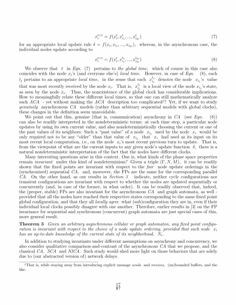
xt+1i = f(xt

i, xti1, ..., xt

i2r) (7)

for an appropriate local update rule δ = f(xi, xi1 , ..., xi2r), whereas, in the asynchronous case, theindividual nodes update according to

xt+1i = f(xt

i, xt1i1, ..., xt2r

i2r) (8)

We observe that t in Eqn. (7) pertains to the global time, which of course in this case alsocoincides with the node xi’s (and everyone else’s) local time. However, in case of Eqn. (8), each

tj pertains to an appropriate local time, in the sense that each xtjij

denotes the node xij ’s value

that was most recently received by the node xi. That is, xtjij

is a local view of the node xij ’s state,as seen by the node xi. Thus, the nonexistence of the global clock has considerable implications.How to meaningfully relate these different local times, so that one can still mathematically analyzesuch ACA - yet without making the ACA description too complicatedj? Yet, if we want to studygenuinely asynchronous CA models (rather than arbitrary sequential models with global clocks),these changes in the definition seem unavoidable.

We point out that this, genuine (that is, communication) asynchrony in CA (see Eqn. (8))can also be readily interpreted in the nondeterministic terms: at each time step, a particular nodeupdates by using its own current value, and also nondeterministically choosing the current or one ofthe past values of its neighbors. Such a “past value” of a node xij used by the node xi would beonly required not to be any “older” than that value of xij that xi had used as its input on itsmost recent local computation, i.e., on the node xi’s most recent previous turn to update. That is,from the viewpoint of what are the current inputs to any given node’s update function δ, there is anatural nondeterministic interpretation of the fact that the nodes have different clocks.

Many interesting questions arise in this context. One is, what kinds of the phase space propertiesremain invariant under this kind of nondeterminism? Given a triple (Γ, N, M), it can be readilyshown that the fixed points are invariant with respect to the fair node update orderings in the(synchronized) sequential CA, and, moreover, the FPs are the same for the corresponding parallelCA. On the other hand, as our results in Section 3 indicate, neither cycle configurations nortransient configurations are invariant with respect to whether the nodes are updated sequentially orconcurrently (and, in case of the former, in what order). It can be readily observed that, indeed,the (proper, stable) FPs are also invariant for the asynchronous CA and graph automata, as well -provided that all the nodes have reached their respective states corresponding to the same fixed pointglobal configuration, and that they all locally agree what (sub)configuration they are in, even if theirindividual local clocks possibly disagree with one another. Therefore, earlier results in [3] on the FPinvariance for sequential and synchronous (concurrent) graph automata are just special cases of this,more general result.

Theorem 3 Given an arbitrary asynchronous cellular or graph automaton, any fixed point configu-ration is invariant with respect to the choice of a node update ordering, provided that each node xi

has an up-to-date knowledge of the current state of its neighborhood, Ni.

In addition to studying invariants under different assumptions on asynchrony and concurrency, wealso consider qualitative comparison-and-contrast of the asynchronous CA that we propose, and theclassical CA, SCA and NICA. Such study would shed more light on those behaviors that are solelydue to (our abstracted version of) network delays.

jThat is, while staying away from introducing explicit message sends and receives, (un)bounded buffers, and thelike.

1787

More generally, communication asynchronous CA, i.e., the various nondeterministic choices fora given automaton that are due to asynchrony, can be shown to subsume all possible behaviorsof the classical and sequential (S)CA with the same corresponding (Γ, N, M). In particular, thenondeterminism that arises from (unbounded) asynchrony subsumes the nondeterminism of a kindstudied in Section 3; but the question arises, exactly how much more expressive the former modelreally is than the latter.

5. Summary and Conclusions

We present herein some early steps in studying cellular automata when the unrealistic assumptionsof perfect synchrony and instantaneous unbounded parallelism are dropped. Motivated by the well-known notion of the sequential interleaving semantics of concurrency, we try to apply this metaphorto parallel CA and thus motivate the study of sequential cellular automata, SCA, and the sequentialinterleavings automata, NICA. In particular, we undertake a comparison and contrast between theSCA/NICA and the classical, parallel CA models when the node update rules are restricted tosimple threshold functions. Concretely, we show that, even in very simplistic cases, this sequential“interleaving semantics” of NICA fails to capture concurrency of the classical CA. One lesson isthat, simple as they may be, the basic local operations (i.e., node updates) in the classical CA cannotalways be considered atomic. That is, the fine-grain parallelism of CA turns out not to be quite fineenough for our purposes. It then appears reasonable - indeed, necessary - to consider a single localnode update to be made of an ordered sequence of the finer elementary operations:

• Fetching all the neighbors’ values (“Receiving”? “Reading shared variables”?)• Updating one’s own state according to the update rule δ (that is, performing the local com-

putation)• Informing the neighbors of the update, i.e., making available one’s new state/value to the

neighbors (“Sending”? “Writing a shared variable”?)

Motivated by these early results on the sequential and parallel threshold CA, and some of theimplications of those results, we next consider various extensions. The central idea is to introduce aclass of genuinely asynchronous CA, and to formally study their properties. This would hopefully,down the road, lead to some significant insights into the fundamental issues related to bounded vs.unbounded asynchrony, formal sequential semantics for parallel and distributed computation, and,on the cellular automata side, to the identification of many of those classical parallel CA phase spaceproperties that are solely or primarily due to the (physically unrealistic) assumption of perfectlysynchronous parallel node updates.

We also find various extensions of the basic CA model to provide a simple, elegant and usefulframework for a high-level study of various global qualitative properties of distributed, parallel andreal-time systems at an abstract and rigorous, yet comprehensive level.

Acknowledgments: The work presented herein was supported by the DARPA IPTO TASKProgram, contract number F30602-00-2-0586. Many thanks to Reza Ziaei (UIUC) for several usefuldiscussions.

1888

References

1. W. Ross Ashby, “Design for a Brain”, Wiley, 19602. C. Barrett and C. Reidys, “Elements of a theory of computer simulation I: sequential CA over random

graphs”, Applied Math. and Computation, vol. 98 (2-3), 19993. C. Barrett, H. Hunt, M. Marathe, S. S. Ravi, D. Rosenkrantz, R. Stearns, and P. Tosic, “Gardens of

Eden and Fixed Points in Sequential Dynamical Systems”, Discrete Math. and Theoretical Comp.Sci. Proc. AA (DM-CCG), July 2001

4. C. Barrett, H. B. Hunt III, M. V. Marathe, S. S. Ravi, D. J. Rosenkrantz, R. E. Stearns, “Reachabilityproblems for sequential dynamical systems with threshold functions”, TCS vol. 295, issues 1-3, pp.41-64, Feb. 2003

5. C. Barrett, H. Mortveit, and C. Reidys, “Elements of a theory of computer simulation II: sequentialdynamical systems”, Applied Math. and Computation, vol. 107 (2-3), 2000

6. C. Barrett, H. Mortveit, and C. Reidys, “Elements of a theory of computer simulation III: equivalenceof sequential dynamical systems”, Applied Math. and Computation, vol. 122 (3), 2001

7. I. Czaja, R. J. van Glabbek, U. Goltz, “Interleaving semantics and action refinement with atomicchoice”, in “Advances in Petri Nets” (G. Rozenberg, ed.), LNCS 609, Springer-Verlag, 1992

8. Max Garzon, ”Models of Massive Parallelism: Analysis of Cellular Automata and Neural Networks”,Springer, 1995

9. R. J. van Glabbek, U. Goltz, “Equivalences and refinement”, Proc. LITP Spring School TheoreticalCS, La Roche-Posay, France (I. Guessarian, ed.), LNCS 469, Springer-Verlag 1990

10. E. Goles, S. Martinez, “Neural and Automata Networks: Dynamical behavior and Applications”,Math. and Its Applications series (vol. 58), Kluwer, 1990

11. E. Goles, S. Martinez (eds.), “Cellular Automata and Complex Systems”, Nonlinear Phenomena andComplex Systems series, Kluwer, 1999

12. Howard Gutowitz (ed.), “Cellular Automata: Theory and Experiment”, The MIT Press / North-Holland, 1991

13. C. A. R. Hoare, “Communicating Sequential Processes”, Prentice Hall, 198514. T. E. Ingerson and R. L. Buvel, “Structure in asynchronous cellular automata”, Physica D: Nonlinear

Phenomena, Volume 10, Issues 1-2, January 198415. S. A. Kauffman, “Emergent properties in random complex automata” (ibid.)16. Robin Milner, ”A Calculus of Communicating Systems”, Springer-Verlag Lecture Notes in Computer

Science (LNCS), 198017. Robin Milner, “Calculi for synchrony and asynchrony”, Theoretical Computer Sci. 25, pp. 267-310,

198318. Robin Milner, “Communication and Concurrency”, Prentice-Hall, 198919. John von Neumann, “Theory of Self-Reproducing Automata”, edited and completed by A. W. Burks,

Univ. of Illinois Press, Urbana, 196620. J. C. Reynolds, “Theories of Programming Languages”, Cambridge Univ. Press, 199821. C. Reidys, “On acyclic orientations and sequential dynamical systems”, Adv. Appl. Math. vol. 27,

200122. Ravi Sethi, “Programming Languages: Concepts & Constructs”, 2nd ed., Addison-Wesley, 1996

1989

23. K. Sutner, “Computation theory of cellular automata”, MFCS98 Satellite Workshop on CA, Brno,Czech Rep., 1998

24. P. Tosic, “A Perspective on the Future of Massively Parallel Computing: Fine-Grain vs. Coarse-GrainParallel Models”, Proc. ACM Computing Frontiers ’04, Ischia, Italy, April 2004

25. P. Tosic, G. Agha, “Characterizing Configuration Spaces of Simple Threshold Cellular Automata”,ACRI’04, Amsterdam, The Netherlands, Oct. 25-28, 2004 (to appear in a Springer-Verlag LNCSvolume)

26. S. Wolfram “Twenty problems in the theory of CA”, Physica Scripta 9, 198527. S. Wolfram (ed.), “Theory and applications of CA”, World Scientific, Singapore, 198628. Stephen Wolfram, “Cellular Automata and Complexity (collected papers)”, Addison-Wesley, 199429. Stephen Wolfram, “A New Kind of Science”, Wolfram Media, Inc., 2002

2090

Online Efficient Predictive Safety Analysis of

Multithreaded Programs

Koushik Sen, Grigore Rosu, Gul AghaDepartment of Computer Science,

University of Illinois at Urbana-Champaign.ksen,grosu,agha@cs.uiuc.edu

Abstract. An automated and configurable technique for runtime safetyanalysis of multithreaded programs is presented, which is able to predictsafety violations from successful executions. Based on a user providedsafety formal specification, the program is automatically instrumentedto emit relevant state update events to an observer, which further checksthem against the safety specification. The events are stamped with dy-namic vector clocks, enabling the observer to infer a causal partial orderon the state updates. All event traces that are consistent with this partialorder, including the actual execution trace, are analyzed on-line and inparallel, and a warning is issued whenever there is a trace violating thespecification. This technique can be therefore seen as a bridge betweentesting and model checking. To further increase scalability, a window inthe state space can be specified, allowing the observer to infer the mostprobable runs. If the size of the window is 1 then only the received ex-ecution trace is analyzed, like in testing; if the size of the window is ∞then all the execution traces are analyzed, such as in model checking.

1 Introduction

In multithreaded systems, threads can execute concurrently communicating witheach other through a set of shared variables, yielding an inherent potential forsubtle errors due to unexpected interleavings. Both heavy and lighter techniquesto detect errors in multithreaded systems have been extensively investigated. Theheavy techniques include traditional formal methods based approaches, such asmodel checking and theorem proving, guaranteeing that a formal model of thesystem satisfies its safety requirements by exploring, directly or indirectly, allpossible thread interleavings. On the other hand, the lighter techniques includetesting, that scales well and is one of the most used approaches to validatesoftware products today.

As part of our overall effort in merging testing and formal methods, aimingat getting some of the benefits of both while avoiding the pitfalls of ad hoctesting and the complexity of full-blown model checking or theorem proving,in this paper we present a runtime verification technique for safety analysis ofmultithreaded systems, that can be tuned to analyze from one trace to all tracesthat are consistent with an actual execution of the program. If all traces arechecked, then it becomes equivalent to online model checking of an abstractmodel of the computation, called the multithreaded computation lattice, whichis extracted from the actual execution trace of the program, like in POTA [10]or JMPaX [14]. If only one trace is considered, then our technique becomesequivalent to checking just the actual execution of the multithreaded program,

91

like in testing or like in other runtime analysis tools like MaC [7] and PaX [5,1]. In general, depending on the application, one can configure a window withinthe state space to be explored, called causality cone, intuitively giving a causal“distance” from the observed execution within which all traces are exhaustivelyverified. An appealing aspect of our technique is that all these traces can beanalyzed online, as the events are received from the running program, and all inparallel at a cost which in the worst case is proportional with both the size ofthe window and the size of the state space of the monitor.

There are three important interrelated components of the proposed runtimeverification technique namely instrumentor, observer and monitor. The codeinstrumentor, based on the safety specification, entirely automatically adds codeto emit events when relevant state updates occur. The observer receives theevents from the instrumented program as they are generated, enqueues them andthen builds a configurable abstract model of the system, known as a computationlattice, on a layer-by-layer basis. As layers are completed, the monitor, which issynthesized automatically from the safety specification, checks them against thesafety specification and then discards them.

The concepts and notions presented in this paper have been experimentedand tested on a practical monitoring system for Java programs, JMPaX 2.0,that extends its predecessor JMPaX [12] in at least four non-trivial novel ways.First, it introduces the technical notion of dynamic vector clock, allowing it toproperly deal with dynamic creation and destruction of threads. Second, thevariables shared between threads do not need to be static anymore: an auto-matic instrumentation technique has been devised that detects automaticallywhen a variable is shared. Thirdly, and perhaps most importantly, the notionof cone heuristic, or global state window, is introduced for the first time in JM-PaX 2.0 to increase the runtime efficiency by analyzing the most likely statesin the computation lattice. Lastly, the presented runtime prediction paradigmis safety formalism independent, in the sense that it allows the user to specifyany safety property whose bad prefixes can be expressed as a non-deterministicfinite automaton (NFA).

2 Monitors for Safety Properties

Safety properties are a very important, if not the most important, class of prop-erties that one should consider in monitoring. This is because once a systemviolates a safety property, there is no way to continue its execution to satisfythe safety property later. Therefore, a monitor for a safety property can pre-cisely say at runtime when the property has been violated, so that an externalrecovery action can be taken. From a monitoring perspective, what is neededfrom a safety formula is a succinct representation of its bad prefixes, which arefinite sequences of states leading to a violation of the property. Therefore, onecan abstract away safety properties by languages over finite words.

Automata are a standard means to succinctly represent languages over finitewords. In what follows we define a suitable version of automata, called monitor,with the property that it has a “bad” state from which it never gets out:

2

92

Definition 1. Let S be a finite or infinite set, that can be thought of as theset of states of the program to be monitored. Then an S-monitor or simply amonitor, is a tuple Mon = 〈M, m0, b, ρ〉, where

– M is the set of states of the monitor;– m0 ∈M is the initial state of the monitor;– b ∈M is the final state of the monitor, also called bad state; and– ρ : M×S → 2M is a non-deterministic transition relation with the property

that ρ(b, Σ) = b for any Σ ∈ S.

Sequences in S⋆, where ǫ is the empty one, are called (execution) traces. A traceπ is said to be a bad prefix inMon iff b ∈ ρ(m0, π), where ρ : 2M×S⋆ → 2M

is recursively defined as ρ(M, ǫ) = M and ρ(M, πΣ) = ρ(ρ(M, π), Σ), whereρ : 2M×S → 2M is defined as ρ(m∪M, Σ) = ρ(m, Σ)∪ρ(M, Σ) and ρ(∅, Σ) =∅, for all finite M ⊆M and Σ ∈ S.

M is not required to be finite in the above definition, but 2M represents theset of finite subsets of M. In practical situations it is often the case that themonitor is not explicitly provided in a mathematical form as above. For example,a monitor can be just any program whose execution is triggered by receivingevents from the monitored program; its state can be given by the values of itslocal variables, and the bad state has some easy to detect property, such as aspecific variable having a negative value.

There are fortunate situations in which monitors can be automatically gen-erated from formal specifications, thus requiring the user to focus on system’sformal safety requirements rather than on low level implementation details. Infact, this was the case in all the experiments that we have performed so far. Wehave so far experimented with requirements expressed either in extended regularexpressions (ERE) or various variants of temporal logics, with both future andpast time. For example, [11, 13] show coinductive techniques to generate min-imal static monitors from EREs and from future time linear temporal logics,respectively, and [6, 1] show how to generate dynamic monitors, i.e., monitorsthat generate their states on-the-fly, as they receive the events, for the safetysegment of temporal logic.

Example 1. Consider a reactive controller that maintains the water level of areservoir within safe bounds. It consists of a water level reader and a valvecontroller. The water level reader reads the current level of the water, calculatesthe quantity of water in the reservoir and stores it in a shared variable w. Thevalve controller controls the opening of a valve by looking at the current quantityof water in the reservoir. A very simple and naive implementation of this systemcontains two threads: T1, the valve controller, and T2, the water level reader.The code snippet for the implementation is given in Fig. 1. Here w is in someproper units such as mega gallons and v is in percentage. The implementationis poorly synchronized and it relies on ideal thread scheduling.

A sample run of the system can be w = 20, v = 40, w = 24, v =50, w = 27, v = 60, w = 31, v = 70. As we will see later in the paper,by a run we here mean a sequence of relevant variable writes. Suppose we are

3

93

Thread T1: Thread T2:

while(true) while(true) if(w > 18) delta = 10; l = readLevel();

else delta = -10; w = calcVolume(l);

for(i=0; i<2; i++) sleep(100);

v = v + delta; setValveOpening(v);

sleep(100);

5

0

1

~p

2

p,~q

q,~r

p,~q

3

p,~q,~r

4

q

q

p,~q

q,~r

q

Fig. 1. Two threads (T1 controls the valve and T2 reads the water level) and a monitor.

interested in a safety property that says “If the water quantity is more than30 mega gallons, then it is the case that sometime in the past water quantityexceeded 26 mega gallons and since then the valve is open by more than 55%and the water quantity never went down below 26 mega gallon”. We can expressthis safety property in two different formalisms: linear temporal logic (LTL) withboth past-time and future-time, or extended regular expressions (EREs) for badprefixes. The atomic propositions that we will consider are p : (w > 26), q : (w >

30), r : (v > 55). The properties can be written as follows:

F1 = (q → ((r ∧ p)S ↑p)) (1)

F2 = ∗¬pp,¬q+(p,¬q,¬rp,¬q∗q+ q∗q,¬r)∗ (2)

The formula F1 in LTL (↑p is a shorthand for “p and previously not p”) statesthat “It is always the case that if (w > 30) then at some time in the past(w > 26) started to be true and since then (r > 55) and (w > 26).” The formulaF2 characterizes the prefixes that make F1 false. In F2 we use p,¬q to denote astate where p and ¬q holds and r may or may not hold. Similarly, representsany state of the system. The monitor automaton for F2 is given also in Fig. 1.

3 Multithreaded Programs

We consider multithreaded systems in which threads communicate with eachother via shared variables. A crucial point is that some variable updates cancausally depend on others. We will describe an efficient dynamic vector clockalgorithm which, given an executing multithreaded program, generates appro-priate messages to be sent to an external observer. Section 4 will show howthe observer, in order to perform its more elaborated analysis, extracts the stateupdate information from such messages together with the causality partial order.

3.1 Multithreaded Executions and Shared Variables

A multithreaded program consists of n threads t1, t2, ..., tn that execute con-currently and communicate with each other through a set of shared variables. A

4

94

multithreaded execution is a sequence of events e1e2 . . . er generated by the run-ning multithreaded program, each belonging to one of the n threads and havingtype internal, read or write of a shared variable. We use e

ji to represent the j-th

event generated by thread ti since the start of its execution. When the thread orposition of an event is not important we can refer to it generically, such as e, e′,etc.; we may write e ∈ ti when event e is generated by thread ti. Let us fix anarbitrary but fixed multithreaded execution, say M, and let S be the set of allvariables that were shared by more than one thread in the execution. There is animmediate notion of variable access precedence for each shared variable x ∈ S:we say e x-precedes e′, written e <x e′, iff e and e′ are variable access events(reads or writes) to the same variable x, and e “happens before” e′, that is, e

occurs before e′ inM. This can be realized in practice by keeping a counter foreach shared variable, which is incremented at each variable access.

3.2 Causality and Multithreaded ComputationsLet E be the set of events occurring inM and let ≺ be the partial order on E :

– eki ≺ el

i if k < l;– e ≺ e′ if there is x ∈ S with e <x e′ and at least one of e, e′ is a write;– e ≺ e′′ if e ≺ e′ and e′ ≺ e′′.

We write e||e′ if e 6≺ e′ and e′ 6≺ e. The tuple (E ,≺) is called the multi-threaded computation associated with the original multithreaded execution M.Synchronization of threads can be easily and elegantly taken into considerationby just generating dummy read/write events when synchronization objects areacquired/released, so the simple notion of multithreaded computation as definedabove is as general as practically needed. A permutation of all events e1, e2, . . .,er that does not violate the multithreaded computation, in the sense that theorder of events in the permutation is consistent with ≺, is called a consistentmultithreaded run, or simply, a multithreaded run.

A multithreaded computation can be thought of as the most general assump-tion that an observer of the multithreaded execution can make about the systemwithout knowing what it is supposed to do. Indeed, an external observer sim-ply cannot disregard the order in which the same variable is modified and usedwithin the observed execution, because this order can be part of the intrinsicsemantics of the multithreaded program. However, multiple consecutive readsof the same variable can be permuted, and the particular order observed in thegiven execution is not critical. As seen in Section 4, by allowing an observer toanalyze multithreaded computations rather than just multithreaded executions,one gets the benefit of not only properly dealing with potential re-orderings ofdelivered messages (e.g., due to using multiple channels in order to reduce themonitoring overhead), but especially of predicting errors from analyzing success-ful executions, errors which can occur under a different thread scheduling.

3.3 Relevant CausalitySome of the variables in S may be of no importance at all for an external observer.For example, consider an observer whose purpose is to check the property “if(x > 0) then (y = 0) has been true in the past, and since then (y > z) was

5

95

always false”; formally, using the interval temporal logic notation in [6], thiscan be compactly written as (x > 0) → [y = 0, y > z). All the other variablesin S except x, y and z are essentially irrelevant for this observer. To minimizethe number of messages, like in [8] which suggests a similar technique but fordistributed systems in which reads and writes are not distinguished, we considera subset R ⊆ E of relevant events and define the R-relevant causality on E as therelation ⊳ :=≺ ∩(R×R), so that e⊳ e′ iff e, e′ ∈ R and e ≺ e′. It is important tonotice though that the other variables can also indirectly influence the relation⊳, because they can influence the relation ≺. We next provide a technique basedon vector clocks that correctly implements the relevant causality relation.

3.4 Dynamic Vector Clock AlgorithmWe provide a technique based on vector clocks [4, 9] that correctly and efficientlyimplements the relevant causality relation. Let V : ThreadId → Nat be a partialmap from thread identifiers to natural numbers. We call such a map a dynamicvector clock (DVC) because its partiality reflects the intuition that threads aredynamically created and destroyed. To simplify the exposition and the imple-mentation, we assume that each DVC V is a total map, where V [t] = 0 wheneverV is not defined on thread t.

We associate a DVC with every thread ti and denote it by Vi. Moreover, weassociate two DVCs V a

x and V wx with every shared variable x; we call the former

access DVC and the latter write DVC. All the DVCs Vi are kept empty at thebeginning of the computation, so they do not consume any space. For DVCs V

and V ′, we say that V ≤ V ′ if and only if V [j] ≤ V ′[j] for all j, and we say thatV < V ′ iff V ≤ V ′ and there is some j such that V [j] < V ′[j]; also, maxV, V ′ isthe DVC with maxV, V ′[j] = maxV [j], V ′[j] for each j. Whenever a threadti with current DVC Vi processes event ek

i , the following algorithm is executed:

1. if eki is relevant, i.e., if ek

i ∈ R, thenVi[i]← Vi[i] + 1

2. if eki is a read of a variable x thenVi ← maxVi, V

wx

V ax ← maxV a

x , Vi3. if ek

i is a write of a variable x thenV w

x ← V ax ← Vi ← maxV a

x , Vi4. if ek

i is relevant thensend message 〈ek

i , i, Vi〉 to observer.

The following theorem states that the DVC algorithm correctly implementscausality in multithreaded programs. This algorithm has been previously pre-sented by the authors in [14, 15] in a less general context, where the number ofthreads is fixed and known a priori. Its proof is similar to that in [15].

Theorem 1. After event eki is processed by thread ti,

– Vi[j] equals the number of relevant events of tj that causally precede eki ; if

j = i and eki is relevant then this number also includes ek

i ;– V a

x [j] equals the number of relevant events of tj that causally precede the mostrecent event that accessed (read or wrote) x; if i = j and ek

i is a relevantread or write of x event then this number also includes ek

i ;

6

96

– V wx [j] equals the number of relevant events of tj that causally precede the

most recent write event of x; if i = j and eki is a relevant write of x then

this number also includes eki .

Therefore, if 〈e, i, V 〉 and 〈e′, j, V ′〉 are two messages sent by dynamic vectorclock algorithm, then e ⊳ e′ if and only if V [i] ≤ V ′[i]. Moreover, if i and j arenot given, then e ⊳ e′ if and only if V < V ′.

4 Runtime Model Generation and Predictive Analysis

In this section we consider what happens at the observer’s site. The observer re-ceives messages of the form 〈e, i, V 〉. Because of Theorem 1, the observer can inferthe causal dependency between the relevant events emitted by the multithreadedsystem. We show how the observer can be configured to effectively analyze allpossible interleavings of events that do not violate the observed causal depen-dency online and in parallel. Only one of these interleavings corresponds to thereal execution, the others being all potential executions. Hence, the presentedtechnique can predict safety violations from successful executions.

4.1 Multithreaded Computation Lattice

Inspired by related definitions in [2], we define the important notions of relevantmultithreaded computation and run as follows. A relevant multithreaded compu-tation, simply called multithreaded computation from now on, is the partial orderon events that the observer can infer, which is nothing but the relation ⊳. A rel-evant multithreaded run, also simply called multithreaded run from now on, isany permutation of the received events which does not violate the multithreadedcomputation. Our major purpose in this paper is to check safety requirementsagainst all (relevant) multithreaded runs of a multithreaded system.

We assume that the relevant events are only writes of shared variables thatappear in the safety formulae to be monitored, and that these events contain apair of the name of the corresponding variable and the value which was writtento it. We call these variables relevant variables. Note that events can changethe state of the multithreaded system as seen by the observer; this is formalizednext. A relevant program state, or simply a program state is a map from relevantvariables to concrete values. Any permutation of events generates a sequenceof program states in the obvious way, however, not all permutations of eventsare valid multithreaded runs. A program state is called consistent if and only ifthere is a multithreaded run containing that state in its sequence of generatedprogram states. We next formalize these concepts.

We letR denote the set of received relevant events. For a given permutation ofevents in R, say e1e2 . . . e|R|, we let ek

i denote the k-th event of thread ti. Then

the relevant program state after the events ek1

1 , ek2

2 , ..., eknn is called a relevant

global multithreaded state, or simply a relevant global state or even just state,and is denoted by Σk1k2...kn . A state Σk1k2...kn is called consistent if and only iffor any 1 ≤ i ≤ n and any li ≤ ki, it is the case that lj ≤ kj for any 1 ≤ j ≤ n

and any lj such that eljj ⊳ eli

i . Let ΣK0 be the initial global state, Σ00...0. Animportant observation is that e1e2 . . . e|R| is a multithreaded run if and only if

7

97

it generates a sequence of global states ΣK0ΣK1 . . . ΣK|R| such that each ΣKr

is consistent and for any two consecutive ΣKr and ΣKr+1 , Kr and Kr+1 differin exactly one index, say i, where the i-th element in Kr+1 is larger by 1 thanthe i-th element in Kr. For that reason, we will identify the sequences of statesΣK0ΣK1 . . . ΣK|R| as above with multithreaded runs, and simply call them runs.

We say that Σ leads-to Σ′, written Σ Σ′, when there is some run in whichΣ and Σ′ are consecutive states. Let ∗ be the reflexive transitive closure ofthe relation . The set of all consistent global states together with the relation

∗ forms a lattice with n mutually orthogonal axes representing each thread.For a state Σk1k2...kn , we call k1 + k1 + · · · kn its level. A path in the lattice is asequence of consistent global states on increasing level, where the level increasesby 1 between any two consecutive states in the path. Therefore, a run is justa path starting with Σ00...0 and ending with Σr1r2...rn , where ri is the totalnumber of events of thread ti. Note that in the above discussion we assumeda fixed number of threads n. In a program where threads can be created anddestroyed dynamically, only those threads are considered that at the end of thecomputation have causally affected the final values of the relevant variables.

Therefore, a multithreaded computation can be seen as a lattice. This lattice,which is called computation lattice and referred to as L, should be seen as anabstract model of the running multithreaded program, containing the relevantinformation needed in order to analyze the program. Supposing that one is ableto store the computation lattice of a multithreaded program, which is a non-trivial matter because it can have an exponential number of states in the lengthof the execution, one can mechanically model-check it against the safety property.

Example 2. Figure 2 shows the causal partial order on relevant events ex-tracted by the observer from the multithreaded execution in Example 1,together with the generated computation lattice. The actual execution,Σ00Σ01Σ11Σ12Σ22Σ23Σ33, is marked with solid edges in the lattice. Besidesits DVC, each global state in the lattice stores its values for the relevant vari-ables, w and v. It can be readily seen on Fig. 2 that the LTL property F1

defined in Example 1 holds on the sample run of the system, and also that it isnot in the language of bad prefixes, F2. However, F1 is violated on some otherconsistent runs, such as Σ00Σ01Σ02Σ12Σ13Σ23Σ33. On this particular run ↑ p

holds at Σ02; however, r does not hold at the next state Σ12. This makes theformula F1 false at the state Σ13. The run can also be symbolically written asppp, qp, q, rp, q, r. In the automaton in Fig. 1, this correspondsto a possible sequence of states 00123555. Hence, this string is accepted by F2

as a bad prefix.

Therefore, by carefully analyzing the computation lattice extracted from asuccessful execution one can infer safety violations in other possible consistentexecutions. Such violations give informative feedback to users, such as the lack ofsynchronization in the example above, and may be hard to find by just ordinarytesting. In what follows we propose effective techniques to analyze the computa-tion lattice. A first important observation is that one can generate it on-the-flyand analyze it on a level-by-level basis, discarding the previous levels. However,

8

98

e6 :<v=70, T1 ,(3,3)>

e4 :<v=60, T1 ,(2,1)>

e3 :< w =27, T2 ,(0,2)>

e2 :<v=50, T1 ,(1,1)>

e1 :< w =24, T2 ,(0,1)>

e5 :< w =31, T2 ,(0,3)>

) 40 , 20 (

) ( 00

= =

=

v w

S L

) 70 , 31 (

, , ) ( 33

= =

=

v w

r q p S L

) 60 , 31 (

, , ) ( 23

= =

=

v w

r q p S L

) 50 , 31 (

, ) ( 13

= =

=

v w

q p S L

) 60 , 27 (

, ) ( 22

= =

=

v w

r p S L

) 40 , 31 (

, ) ( 03

= =

=

v w

q p S L

) 50 , 27 (

) ( 12

= =

=

v w

p S L

) 60 , 24 (

) ( 21

= =

=

v w

r S L

) 40 , 27 (

) ( 02

= =

=

v w

p S L

) 50 , 24 (

) ( 11

= =

=

v w

S L

) 40 , 24 (

) ( 01

= =

=

v w

S L

Fig. 2. Computation Lattice

even if one considers only one level, that can still contain an exponential numberof states in the length of the current execution. A second important observationis that the states in the computation lattice are not all equiprobable in prac-tice. By allowing a user configurable window of most likely states in the latticecentered around the observed execution trace, the presented technique becomesquite scalable, requiring O(wm) space and O(twm) time, where w is the size ofthe window, m is the size of the bad prefix monitor of the safety property, andt is the size of the monitored execution trace.

4.2 Level By Level Analysis of the Computation LatticeA naive observer of an execution trace of a multithreaded program would justcheck the observed execution trace against the monitor for the safety property,sayMon like in Definition 1, and would maintain at each moment a set of states,say MonStates inM. When a new event generating a new global state Σ arrives,it would replace MonStates by ρ(MonStates, Σ). If the bad state b will ever be inMonStates then a property violation error would be reported, meaning that thecurrent execution trace led to a bad prefix of the safety property. Here we assumethat the events are received in the order in which they are emitted, and also thatthe monitor works over the global states of the multithreaded programs.

A smart observer, as said before, will analyze not only the observed executiontrace, but also all the other consistent runs of the multithreaded system, thusbeing able to predict violations from successful executions. The observer receivesthe events from the running multithreaded program in real-time and enqueues

9

99

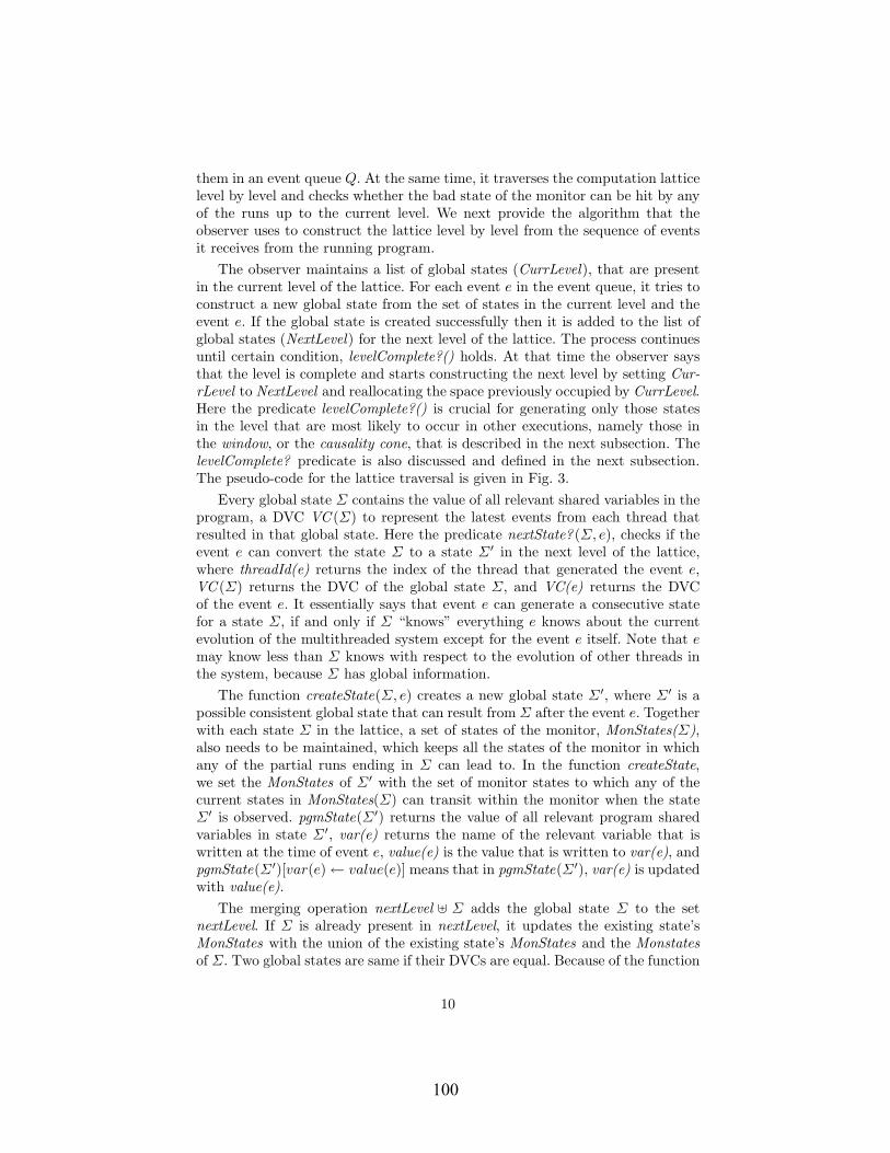
them in an event queue Q. At the same time, it traverses the computation latticelevel by level and checks whether the bad state of the monitor can be hit by anyof the runs up to the current level. We next provide the algorithm that theobserver uses to construct the lattice level by level from the sequence of eventsit receives from the running program.

The observer maintains a list of global states (CurrLevel), that are presentin the current level of the lattice. For each event e in the event queue, it tries toconstruct a new global state from the set of states in the current level and theevent e. If the global state is created successfully then it is added to the list ofglobal states (NextLevel) for the next level of the lattice. The process continuesuntil certain condition, levelComplete?() holds. At that time the observer saysthat the level is complete and starts constructing the next level by setting Cur-rLevel to NextLevel and reallocating the space previously occupied by CurrLevel.Here the predicate levelComplete?() is crucial for generating only those statesin the level that are most likely to occur in other executions, namely those inthe window, or the causality cone, that is described in the next subsection. ThelevelComplete? predicate is also discussed and defined in the next subsection.The pseudo-code for the lattice traversal is given in Fig. 3.

Every global state Σ contains the value of all relevant shared variables in theprogram, a DVC VC (Σ) to represent the latest events from each thread thatresulted in that global state. Here the predicate nextState? (Σ, e), checks if theevent e can convert the state Σ to a state Σ′ in the next level of the lattice,where threadId(e) returns the index of the thread that generated the event e,VC (Σ) returns the DVC of the global state Σ, and VC(e) returns the DVCof the event e. It essentially says that event e can generate a consecutive statefor a state Σ, if and only if Σ “knows” everything e knows about the currentevolution of the multithreaded system except for the event e itself. Note that e

may know less than Σ knows with respect to the evolution of other threads inthe system, because Σ has global information.

The function createState(Σ, e) creates a new global state Σ′, where Σ′ is apossible consistent global state that can result from Σ after the event e. Togetherwith each state Σ in the lattice, a set of states of the monitor, MonStates(Σ),also needs to be maintained, which keeps all the states of the monitor in whichany of the partial runs ending in Σ can lead to. In the function createState,we set the MonStates of Σ′ with the set of monitor states to which any of thecurrent states in MonStates(Σ) can transit within the monitor when the stateΣ′ is observed. pgmState(Σ′) returns the value of all relevant program sharedvariables in state Σ′, var(e) returns the name of the relevant variable that iswritten at the time of event e, value(e) is the value that is written to var(e), andpgmState(Σ′)[var(e)← value(e)] means that in pgmState(Σ′), var(e) is updatedwith value(e).

The merging operation nextLevel ⊎ Σ adds the global state Σ to the setnextLevel. If Σ is already present in nextLevel, it updates the existing state’sMonStates with the union of the existing state’s MonStates and the Monstatesof Σ. Two global states are same if their DVCs are equal. Because of the function

10

100

levelComplete?, it may be often the case that the analysis procedure moves fromthe current level to the next one before it is exhaustively explored. That meansthat several events in the queue, which were waiting for other events to arrive inorder to generate new states in the current level, become unnecessary so they canbe discarded. The function removeUselessEvents(CurrLevel,Q) removes from Q

all the events that cannot contribute to the construction of any state at the nextlevel. To do so, it creates a DVC Vmin whose each component is the minimumof the corresponding component of the DVCs of all the global states in the setCurrLevel. It then removes all the events in Q whose DVCs are less than or equalto Vmin. This function makes sure that we do not store any unnecessary events.

while(not end of computation)

Q← enqueue(Q, NextEvent())

while(constructLevel())

boolean constructLevel()

for each e ∈ Q

if Σ ∈ CurrLevel and nextState?(Σ, e)

NextLevel ← NextLevel ⊎ createState(Σ, e)

if levelComplete?(NextLevel , e, Q)

Q← removeUselessEvents(CurrLevel , Q)

CurrLevel ← NextLevel

return true

return false

boolean nextState?(Σ, e)

i← threadId(e);

if (∀j 6= i : VC (Σ)[j] ≥ VC (e)[j] and

VC (Σ)[i] + 1 = VC (e)[i]) return true

return false

State createState(Σ, e)

Σ′ ← new copy of Σ

j ← threadId(e); VC (Σ′)[j]← VC (Σ)[j]+1

pgmState(Σ′)[var(e)← value(e)]

MonStates(Σ′)← ρ(MonStates(Σ), Σ′)

if b ∈ MonStates(Σ′)

output ′property may be violated′

return Σ′

Fig. 3. Level-by-level traversal.

The observer runs in a looptill the computation ends. In theloop the observer waits for thenext event from the running in-strumented program and enqueuesit in Q whenever it becomes avail-able. After that the observer runsthe function constructLevel in aloop till it returns false. If the func-tion constructLevel returns falsethen the observer knows that thelevel is not completed and itneeds more events to complete thelevel. At that point the observeragain starts waiting for the nextevent from the running programand continues with the loop. Thepseudo-code for the observer isgiven at the top of Fig. 3.

4.3 Causality Cone

Heuristic

In a given level of a computationlattice, the number of states canbe large; in fact, exponential in thelength of the trace. In online anal-ysis, generating all the states in alevel may not be feasible. However,note that some states in a level canbe considered more likely to occurin a consistent run than others. Forexample, two independent events

that can possibly permute may have a huge time difference. Permuting thesetwo events would give a consistent run, but that run may not be likely to takeplace in a real execution of the multithreaded program. So we can ignore such a

11

101

permutation. We formalize this concept as causality cone, or window, and exploitit in restricting our attention to a small set of states in a given level.

In what follows we assume that the events are received in an order in whichthey happen in the computation. This is easily ensured by proper instrumen-tation. Note that this ordering gives the real execution of the program and itrespects the partial order associated with the computation. This execution willbe taken as a reference in order to compute the most probable consistent runsof the system.

If we consider all the events generated by the executing distributed programas a finite sequence of events, then a lattice formed by any prefix of this sequenceis a sublattice of the computation lattice L. This sublattice, say L′ has thefollowing property: if Σ ∈ L′, then for any Σ′ ∈ L if Σ′

∗ Σ then Σ′ ∈ L′. We

can see this sublattice as a portion of the computation lattice L enclosed by acone. The height of this cone is determined by the length of the current sequenceof events. We call this causality cone. All the states in L that are outside thiscone cannot be determined from the current sequence of events. Hence, they areoutside the causal scope of the current sequence of events. As we get more eventsthis cone moves down by one level.

w =3

< w =3

w

Fig. 4. Causality Cones

If we compute a DVC Vmax whose each component is the maximum of thecorresponding component of the DVCs of all the events in the event queue, thenthis represents the DVC of the global state appearing at the tip of the cone. Thetip of the cone traverses the actual execution run of the program.

To avoid the generation of possibly exponential number of states in a givenlevel, we consider a fixed number, say w, most probable states in a given level. In

12

102

a level construction we say the level is complete once we have generated w statesin that level. However, a level may contain less than w states. Then the levelconstruction algorithm gets stuck. Moreover, we cannot determine if a level hasless than w states unless we see all the events in the complete computation. Thisis because we do not know the total number of threads that participate in thecomputation beforehand. To avoid this scenario we introduce another parameterl, the length of the current event queue. We say that a level is complete if we haveused all the events in the event queue for the construction of the states in thecurrent level and the length of the queue is l and we have not crossed the limit w

on the number of states. The pseudo-code for levelComplete? is given in Fig. 5

boolean levelComplete?(NextLevel, e, Q)

if size(NextLevel) ≥ w then

return true;

else if e is the last event in Q

and size(Q) == l then

return true;

else return false;

Fig. 5. levelComplete? predicate

Note, here l corresponds to thenumber of levels of the sublat-tice that be constructed from theevents in the event queue Q. On theother hand, the level of this sublat-tice with the largest level numberand having at least w global statesrefers to the CurrLevel in the al-gorithm.

5 ImplementationWe have implemented these new techniques, in version 2.0 of the tool Java Mul-tiPathExplorer (JMPaX)[12], which has been designed to monitor multithreadedJava programs. The current implementation is written in Java and it removes therestriction that all the shared variables of the multithreaded program are staticvariables of type int. The tool has three main modules, the instrumentationmodule, the observer module and the monitor module.

The instrumentation program, named instrument, takes a specification fileand a list of class files as command line arguments. An example is

java instrument spec A.class B.class C.class

where the specification file spec contains a list of named formulae written ina suitable logic. The program instrument extracts the name of the relevantvariables from the specification and instruments the classes, provided in theargument, as follows:

i) For each variable x of primitive type in each class it adds access and writeDVCs, namely _access_dvc_x and _write_dvc_x, as new fields in the class.

ii) It adds code to associate a DVC with every newly created thread;iii) For each read and write access of a variable of primitive type in any class,

it adds codes to update the DVCs according to the algorithm mentioned inSection 3.4;

iv) It adds code to call a method handleEvent of the observer module at everywrite of a relevant variable.

The instrumentation module uses BCEL [3] Java library to modify Java classfiles. We use the BCEL library to get a better handle for a Java classfile.

13

103

The observer module, that takes two parameters w and l, generates thelattice level by level when the instrumented program is executed. Whenever thehandleEvent method is invoked it enqueues the event passed as argument tothe method handleEvent. Based on the event queue and the current level ofthe lattice it generates the next level of the lattice. In the process it invokesnextStates method (corresponding to ρ in a monitor) of the monitor module.

The monitor module reads the specification file written either as an LTLformula or a regular expression and generates the non-deterministic automatoncorresponding to the formula or the regular expression. It provides the methodnextStates as an interface to the observer module. The method raises an excep-tion if at any point the set of states returned by nextStates contain the “bad”state of the automaton. The system being modular, user can plug in his/her ownmonitor module for his/her logic of choice.

Since in Java synchronized blocks cannot be interleaved, so correspondingevents cannot be permuted, locks are considered as shared variables and a writeevent is generated whenever a lock is acquired or released. This way, a causaldependency is generated between any exit and any entry of a synchronized block,namely the expected happens-before relation. Java synchronization statementsare handled exactly the same way, that is, the shared variable associated tothe synchronization object is written at the entrance and at the exit of thesynchronized region. Condition synchronizations (wait/notify) can be handledsimilarly, by generating a write of a dummy shared variable by both the notifyingthread before notification and by the notified thread after notification.

6 Conclusion and Future Work

A formal runtime predictive analysis technique for multithreaded systems hasbeen presented in this paper, in which multiple threads communicating by sharedvariables are automatically instrumented to send relevant events, stamped bydynamic vector clocks, to an external observer which extracts a causal partialorder on the global state, updates and thereby builds an abstract runtime modelof the running multithreaded system. Analyzing this model on a level by levelbasis, the observer can infer effectively from successful execution of the observedsystem when basic safety properties can be violated by other executions. At-tractive future work includes predictions of liveness violations and predictionsof datarace and deadlock conditions.

7 Acknowledgments

The work is supported in part by the Defense Advanced Research Projects Agency (theDARPA IPTO TASK Program, contract number F30602-00-2-0586, the DARPA IXONEST Program, contract number F33615-01-C-1907), the ONR Grant N00014-02-1-0715, the Motorola Grant MOTOROLA RPS #23 ANT, and the joint NSF/NASAgrant CCR-0234524.

References

1. H. Barringer, A. Goldberg, K. Havelund, and K. Sen. Rule-Based Run-time Verification. In Proceedings of Fifth International VMCAI con-

14

104

ference (VMCAI’04) (To appear in LNCS), January 2004. Download:http://www.cs.man.ac.uk/cspreprints/PrePrints/cspp24.pdf.

2. H. W. Cain and M. H. Lipasti. Verifying sequential consistency using vector clocks.In Proceedings of the 14th annual ACM Symposium on Parallel Algorithms andArchitectures, pages 153–154. ACM, 2002.

3. M. Dahm. Byte code engineering with the bcel api. Technical Report B-17-98,Freie Universit at Berlin, Institut fur Informatik, April 2001.

4. C. J. Fidge. Partial orders for parallel debugging. In Proceedings of the 1988 ACMSIGPLAN and SIGOPS workshop on Parallel and Distributed debugging, pages183–194. ACM, 1988.

5. K. Havelund and G. Rosu. Monitoring Java Programs with Java PathExplorer. InProceedings of the 1st Workshop on Runtime Verification (RV’01), volume 55 ofElectronic Notes in Theoretical Computer Science. Elsevier Science, 2001.

6. K. Havelund and G. Rosu. Synthesizing monitors for safety properties. In Toolsand Algorithms for Construction and Analysis of Systems (TACAS’02), volume2280 of Lecture Notes in Computer Science, pages 342–356. Springer, 2002.

7. M. Kim, S. Kannan, I. Lee, and O. Sokolsky. Java-MaC: a Run-time AssuranceTool for Java. In Proceedings of the 1st Workshop on Runtime Verification (RV’01),volume 55 of Electronic Notes in Theoretical Computer Science. Elsevier Science,2001.

8. K. Marzullo and G. Neiger. Detection of global state predicates. In Proceedingsof the 5th International Workshop on Distributed Algorithms (WADG’91), volume579 of Lecture Notes in Computer Science, pages 254–272. Springer-Verlag, 1991.

9. F. Mattern. Virtual time and global states of distributed systems. In Parallel andDistributed Algorithms: proceedings of the International Workshop on Parallel andDistributed Algorithms, pages 215–226. Elsevier, 1989.

10. A. Sen and V. K. .Garg. Partial order trace analyzer (pota) for distrubted pro-grams. In Proceedings of the 3rd Workshop on Runtime Verification (RV’03),Electronic Notes in Theoretical Computer Science, 2003.

11. K. Sen and G. Rosu. Generating optimal monitors for extended regular expressions.In Proceedings of the 3rd Workshop on Runtime Verification (RV’03), volume 89of ENTCS, pages 162–181. Elsevier Science, 2003.

12. K. Sen, G. Rosu, and G. Agha. Java MultiPathExplorer (JMPaX 2.0). Download:http://fsl.cs.uiuc.edu/jmpax.

13. K. Sen, G. Rosu, and G. Agha. Generating Optimal Linear Temporal Logic Mon-itors by Coinduction. In Proceedings of 8th Asian Computing Science Conference(ASIAN’03), volume 2896 of Lecture Notes in Computer Science, pages 260–275.Springer-Verlag, December 2003.

14. K. Sen, G. Rosu, and G. Agha. Runtime safety analysis of multithreaded pro-grams. In Proceedings of 4th joint European Software Engineering Conferenceand ACM SIGSOFT Symposium on the Foundations of Software Engineering(ESEC/FSE’03). ACM, 2003.

15. K. Sen, G. Rosu, and G. Agha. Runtime safety analysis of multithreaded pro-grams. Technical Report UIUCDCS-R-2003-2334, University of Illinois at UrnabaChampaign, April 2003.

15

105

A Flexible Coordination Framework for Application-Oriented Matchmaking and Brokering Services

Myeong-Wuk Jang, Amr M.E. Ahmed, Gul Agha Open Systems Laboratory

Department of Computer Science University of Illinois at Urbana-Champaign

mjang, amrmomen, agha@uiuc.edu

Abstract

An important problem for agents in open multiagent systems is how to find agents that match certain criteria. A number of middle agent services, such as matchmaking and brokering services, have been proposed to address this problem. However, the search capabilities of such services are relatively limited since the match criteria they use are relatively inflexible. We propose ATSpace, a middle agent to support application-

oriented matchmaking and brokering services. Application agents in ATSpace deliver their own search algorithms to a public tuple space which holds agent property data; the tuple space executes the search algorithms on this data. We show how the ATSpace model increases the dynamicity and flexibility of middle agent services. Unfortunately, the model also introduces security threats: the data and access control restrictions in ATSpace may be compromised, and system availability may be affected. We describe some mechanisms to mitigate these security threats.

Keywords: Agent Coordination, Agent Interaction, Middle Agents, Brokering Services, Matchmaking Services.

1. Introduction In multiagent systems, agents need to communicate with each other to accomplish their goals. An important problem in open multiagent systems is the connection problem: how to find agents that match given criteria [Dav83]. When agents are designed or owned by the same organization,

- 1 - 106

developers may be able to design agents which explicitly know the names of other agents that they need to communicate with. However in open systems, because different agents may dynamically enter or leave a system, it is generally not feasible to let agents know the names of all other agents that they need to communicate with at some point.

For solving the connection problem, Decker classifies middle agent services as either matchmaking (also called Yellow Page) services or brokering services [Dec96, Syc97]. Matchmaking services (e.g. Directory Facilitator in FIPA platforms [Fip02]) are passive services whose goal is to provide a client agent with a list of names of agents whose properties match its supplied criteria. The agent may later contact the matched agents to request services. On the other hand, brokering services (e.g. ActorSpace [Cal94]) are active services that directly deliver a message (or a request) to the relevant agents on their clients’ behalf.

In both types of services, an agent advertises itself by sending a message which contains its name and a description of its characteristics to a middle agent. A middle agent may be implemented on top of a tuple space model such as Linda [Car89]; this involves imposing constraints on the format of the stored tuples and using Linda-supported primitives. Specifically, to implement matchmaking and brokering services on top of Linda, a tuple template may be used by the client agent to specify the matching criteria. However, the expressive power of a template is very limited; it consists of value constraints for its actual parameters and type constraints for its formal parameters. In order to overcome this limitation, Callsen's ActorSpace implementation used regular expressions in its search template [Agh93, Cal94]. Even though this implementation increased expressivity, its capability is still limited by the power of its regular expressions.

We propose ATSpace1 (Active Tuple Spaces) to empower agents with the ability to provide arbitrary application-oriented search algorithms to a middle agent for execution on the tuple space. While ATSpace increases the dynamicity and flexibility of the tuple space model, it also introduces some security threats as codes developed by different groups with different interests are executed in the same space. We will discuss the implication of these threats and how they may be mitigated.

This paper is organized as follows. Section 2 explains the ATSpace architecture and introduces its primitives. Section 3 describes security threats occurred in ATSpace and addresses how to resolve them. Section 4 illustrates the power of the new primitives by describing experiments with using ATSpace on UAV (Unmanned Aerial Vehicle) simulations. Section 5 evaluates the

1 We will use ATSpace to refer the model for a middle agent to support application-oriented service, while we

use an atSpace to refer an instance of ATSpace.

- 2 - 107

performance of ATSpace and compares it with a general middle agent. Section 6 discusses related work, and finally, we conclude this paper with a summary of our research and future work.

2. ATSpace

2.1 A MOTIVATIVE EXAMPLE

We present a simple example to motivate the ATSpace model. In general, a tuple space user with a complex matching query is faced with the following two problems:

1. Expressiveness problem because a matching query cannot be expressed using the tuple space primitives.

2. Incomplete information problem because evaluating a matching query requires information which is not available for a tuple space manager.

For example, assume that a tuple space has information about seller agents and the prices of the

products they sell; each tuple has the following attributes (seller name, seller city, product name, product price). Buyer agents can access the tuple space in order to find

seller agents that sell, for instance, computers or printers. Also, a buyer agent wants to execute the following query:

Q1: What are the best two (in terms of prices) sellers that offer computers and whose locations are roughly within 50 miles from me?

A generic tuple space may not support the request of this buyer agent because, firstly, it may not support the “best two” primitive (problem 1), and secondly, it may not have information about the distance between cities (problem 2). Faced with these difficulties the buyer agent with the query Q1 has to transform it to a tuple template style query (Q2) to be accepted by the general tuple space. This query Q2 will retrieve a superset of the data that should have been retrieved by Q1. Q2: Find all tuples about seller agents that sell computers.

The buyer agent then evaluates its own search algorithm on the returned data to find tuples that

- 3 - 108

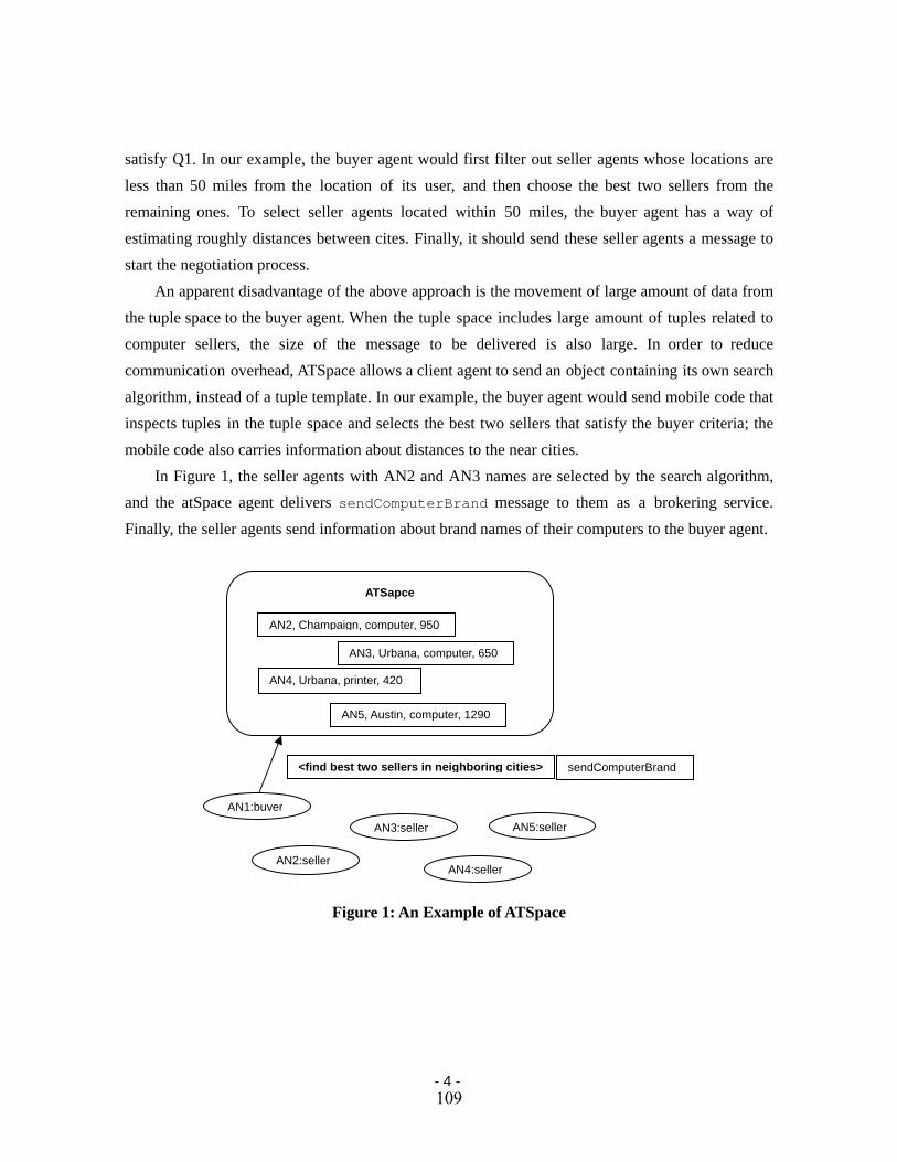
satisfy Q1. In our example, the buyer agent would first filter out seller agents whose locations are less than 50 miles from the location of its user, and then choose the best two sellers from the remaining ones. To select seller agents located within 50 miles, the buyer agent has a way of estimating roughly distances between cites. Finally, it should send these seller agents a message to start the negotiation process.

An apparent disadvantage of the above approach is the movement of large amount of data from the tuple space to the buyer agent. When the tuple space includes large amount of tuples related to computer sellers, the size of the message to be delivered is also large. In order to reduce communication overhead, ATSpace allows a client agent to send an object containing its own search algorithm, instead of a tuple template. In our example, the buyer agent would send mobile code that inspects tuples in the tuple space and selects the best two sellers that satisfy the buyer criteria; the mobile code also carries information about distances to the near cities.

In Figure 1, the seller agents with AN2 and AN3 names are selected by the search algorithm, and the atSpace agent delivers sendComputerBrand message to them as a brokering service.

Finally, the seller agents send information about brand names of their computers to the buyer agent.

ATSapce

AN2, Champaign, computer, 950

AN3, Urbana, computer, 650

AN4, Urbana, printer, 420

AN5, Austin, computer, 1290

Figure 1: An Example of ATSpace

<find best two sellers in neighboring cities> sendComputerBrand

AN1:buyer

AN5:sellerAN3:seller

AN2:seller AN4:seller

- 4 - 109

2.2 OVERALL ARCHITECTURE ATSpace consists of three components: a tuple space, a message queue, and a tuple space manager (see Figure 2).

ATSpace

Tuple Space message queue

Figure 2: Basic Architecture of ATSpace

The tuple space is used as a shared pool for agent tuples, npppa ,...,,, 21 , which consists of a

name field, a, and a property part, P = p1, p2, …, pn where n ≥ 1; each tuple represents an agent whose name is given by the first field and whose characteristics are given by the subsequent fields. ATSpace enforces the rule that there cannot be more than one agent tuples whose agent names and property fields are identical. However, an agent may register itself with different properties (multiple tuples with the same name field), and different agents may register themselves with the same property fields (multiple tuples with the same property part).

)]..()..&(&)..()..[(:, atatPtPtPtPtatatjitt jijijijiji ≠→=≠→=→≠∀

The message queue contains input messages that are received from other agents. Messages are classified into two types: data input messages and service request messages. A data input message includes a new agent tuple for insertion into the tuple space. A service request message includes either a tuple template or a mobile object. The template (or, alternately, the object) is used to search for agents with the appropriate agent tuples. A service request message may optionally contain another field, called the service call message field, to facilitate the brokering service. A mobile

tuple

tuple

tuple

tupleTuple Space

Manager ask service agents(brokering)

return names (matchmaking)

msgmsgmsg

- 5 - 110

object is an object that is provided by a service-requesting agent or client agent; such objects have pre-defined public methods, such as find. The find method is called by the tuple space manager

with tuples in its atSpace as a parameter, and this method returns names of agents selected by the search algorithm specified in the mobile object.

The tuple space manager retrieves names of service agents whose properties match a tuple template or which are selected by a mobile object. In case of a matchmaking service, it returns the names to the client agent. In case of a brokering service, it forwards the service call message supplied by the client agent to the service agents.

2.3 OPERATION PRIMITIVES

General Tuple Space Primitives The ATSpace model supports three basic primitives: write, read, and take. write is used to register an agent tuple into an atSpace, read is used to retrieve an agent tuple that matches a given criteria, and take is used to retrieve a matched agent tuple and remove it from the atSpace. When

there are more than one agent tuples whose properties are matched with the given criteria, one of them is randomly selected by the agent tuple manager. When there is no a matched tuple, these primitives return immediately with an exception. In order to retrieve all agent tuples that match a given criteria, readAll or takeAll primitives should be used. The format2 of these primitives is

as follows:

void write(AgentName anATSpace, TupleData td); AgentTuple read(AgentName anATSpace, TupleTemplate tt); AgentTuple take(AgentName anATSpace, TupleTemplate tt); AgentTuple[] readAll(AgentName anATSpace, TupleTemplate tt); AgentTuple[] takeAll(AgentName anATSpace, TupleTemplate tt);

where AgentName, TupleData, AgentTuple, and TupleTemplate are data objects defined in

ATSpace. A data object denotes an object that includes only methods to set and retrieve its member variables. When one of these primitives is called in an agent, the agent class handler creates a corresponding message and sends it to the atSpace specified as the first parameter, anATSpace. The write primitive causes a data input message while the others cause service request messages. Note that the write primitive does not include an agent tuple but a tuple that contains only the agent’s

2 The current ATSpace implementation is developed in the Java programming language, and hence, we use the Java syntax to express primitives.

- 6 - 111

properties. This is to avoid the case where an agent tries to register a property using another agent name to an atSpace. This tuple is then converted to an agent tuple with the name of the sender agent before the agent tuple is inserted to an atSpace.

In some applications, updating agent tuples happens very often. For such applications, availability and integrity are of great importance. Availability insures that at least one agent tuple exist at any time whereas integrity insures that old and new agent data do not exist simultaneously in an atSpace. Implementing the update request using two tuple space primitives, take and write, could result in one of these properties not being satisfied. If update is implemented using take followed by write, then availability is not met. On the other hand, if update is implemented using write followed by take, integrity is violated for a small amount of time. Therefore, ATSpace provides the update primitive to insure that take and write operations are performed as one

atomic operation.

void update(AgentName anATSpace, TupleTemplate tt, TupleData td);

Matchmaking and Brokering Service Primitives

In addition, ATSpace also provides primitives for middle agent services: searchOne and searchAll for matchmaking services, and deliverOne and deliverAll for brokering services.

Primitives for matchmaking are as follows:

AgentName searchOne(AgentName anATSpace, TupleTemplate tt); AgentName searchOne(AgentName anATSpace, MobileObject ao); AgentName[] searchAll(AgentName anATSpace, TupleTemplate tt); AgentName[] searchAll(AgentName anATSpace, MobileObject ao);

The searchOne primitive is used to retrieve the name of a service agent that satisfies a given criteria, whereas the searchAll primitive is used to retrieve all names of service agents that match

a given property. Primitives for brokering service are as follows:

void deliverOne(AgentName anATSpace, TupleTemplate tt, Message msg); void deliverOne(AgentName anATSpace, MobileObject ao, Message msg); void deliverAll(AgentName anATSpace, TupleTemplate tt, Message msg); void deliverAll(AgentName anATSpace, MobileObject ao, Message msg);

The deliverOne primitive is used to forward a specified service call message msg to the service agent that matches the given criteria, whereas the deliverAll primitive is used to send

this message to all such service agents.

- 7 - 112

Note that our matchmaking and brokering service primitives allow agents to use mobile objects

to support application-oriented search algorithm. We call matchmaking or brokering services used with mobile objects active matchmaking or brokering services. MobileObject is an abstract class

that defines the interface methods between a mobile object and an atSpace. One of these methods is find, which may be used to provide the search algorithm to an atSpace. The format of the find

method is defined as follows:

AgentName[] find(final AgentTuple[] ataTuples);

Service Specific Request Primitive

One drawback of the previous brokering primitives (deliverOne and deliverAll) is that they

cannot support service-specific call messages. In some situations, a client agent cannot supply an atSpace with a service call message to be delivered to a service agent beforehand because it needs to examine the service agent properties first. Another drawback of the deliverAll primitive is that

it stipulates that the same message should be sent to all service agents that match the supplied criteria. In some situations a client agent needs to send different messages to each service agent, depending on the service agent’s properties. A client agent with any of the above requirements can use neither brokering services with tuple templates nor active brokering services with mobile objects. Therefore, the agent has to use the readAll primitive to retrieve relevant agent tuples and

then create appropriate service call messages to send service agents selected. However, this approach suffers from the same problems as a general tuple space does.

To address the above shortcomings, we introduce the exec primitives. This primitive allows a

client agent to supply a mobile object to an atSpace; the supplied mobile object has to implement the doAction method. When the method is called by an atSpace with agent tuples, it examines the

properties of agents using the client agent application logic, creates different service call messages according to the agent properties, and then returns a list of agent messages to the atSpace to deliver the service call messages to the selected agents. Note that each agent message consists of the name of a service agent as well as a service call message to be delivered to the service agent. The formats of exec primitive and the doAction method are as follows.

void exec(AgentName anATSpace, MobileObject ao); AgentMessage[] doAction(AgentTuple[] ataTuples);

- 8 - 113

3. SECURITY ISSUES

By allowing a mobile object to be supplied by an application agent, ATSpace supports application-oriented matchmaking and brokering services, which increases the flexibility and dynamicity of the tuple space model. However, it also introduces new security threats; we address some of these security threats and describe some ways to mitigate them. There are three important types of security issues for ATSpace:

Data Integrity: A mobile object may not modify tuples owned by other agents. Denial of Service: A mobile object may not consume two much processing time or space

of an atSpace, and a client agent may not repeatedly send mobile objects, thus overloading an atSpace.

Illegal Access: A mobile object may not carry out unauthorized access or illegal operations.

We address the data integrity problem by blocking attempts to modify tuples. When a mobile

object is executed by a tuple space manager, the manager makes a deep copy of tuples and then sends the copy to the find or doAction method of the mobile object. Therefore, even when a

malicious agent changes some tuples, the original tuples are not affected by the modification. However, when the number of tuples in a tuple space is very large, this solution requires extra memory and computational resources. For better performance, the creator of an atSpace may select the option of delivering to mobile objects a shallow copy of the original tuples instead of a deep copy, although this will violate the integrity of tuples if an agent tries to delete or change tuples. We are currently investigating under what conditions a use of a shallow copy may be sufficient.

To address denial of service by consuming all processor cycles, we deploy user-level thread scheduling. Figure 3 depicts the extended architecture of ATSpace. When a mobile object arrives, the object is executed as a thread, and its priority is set to high. If the thread executes for a long time, its priority is continually downgraded. Moreover, if the running time of a mobile object exceeds a certain limit, it may be destroyed by the Tuple Space Manager; in this case, a message is sent to the sender agent of the mobile object to inform it about the destruction of the object. To incorporate these restrictions, we have extended the architecture of ATSpace by implementing job queues--thus making their semantics similar to that of actors. Other denial of service issues are still our on-going research.

- 9 - 114

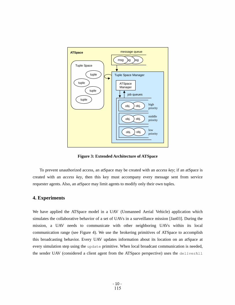
message queueATSpace

Figure 3: Extended Architecture of ATSpace To prevent unauthorized access, an atSpace may be created with an access key; if an atSpace is

created with an access key, then this key must accompany every message sent from service requester agents. Also, an atSpace may limit agents to modify only their own tuples.

4. Experiments

We have applied the ATSpace model in a UAV (Unmanned Aerial Vehicle) application which simulates the collaborative behavior of a set of UAVs in a surveillance mission [Jan03]. During the mission, a UAV needs to communicate with other neighboring UAVs within its local communication range (see Figure 4). We use the brokering primitives of ATSpace to accomplish this broadcasting behavior. Every UAV updates information about its location on an atSpace at every simulation step using the update primitive. When local broadcast communication is needed, the sender UAV (considered a client agent from the ATSpace perspective) uses the deliverAll

Tuple Space Manager

Tuple Space

tuple

tuple

tuple

tuple

ATSpace Manager

msgmsgmsg

job queues

high obj.obj.priority

middleobj.obj. priority

low obj.obj. priority

- 10 - 115

primitive and supplies as a parameter a mobile object3 that contains its location and communication range. When this mobile object is executed in the atSpace, the find method is called by the tuple space manager to find relevant receiver agents. The find method computes distances between the

sender UAV and other UAVs to find neighboring ones within the given communication range. When the tuple space manager receives names of service agents, neighboring UAVs in this example, from the mobile object, it delivers the service call message given by the client agent--the sender UAV in this example--to them.

Figure 4: Simulation of Local Broadcast Communication We also use ATSpace to simulate the behavior of UAV radar sensors. Each UAV should detect

targets within its sensing radar range (see Figure 5). The SensorSimulator, which is the simulator component responsible for accomplishing this behavior, uses the exec primitive to implement this task. The mobile object4 supplied with the exec primitive computes distances between UAVs and

targets, and decides neighboring targets for each UAV. It then creates messages each of which consists of the name of its receiver UAV and a service call message to be sent its receiver UAV agent. This service call message is simply the environment model around this UAV (neighboring targets in our domain). Finally, the mobile object returns these set of messages to the tuple space manager which in turn sends them to respective agents.

3 The code for this mobile object is in Appendix A. 4 The code for this mobile object is in Appendix B.

- 11 - 116

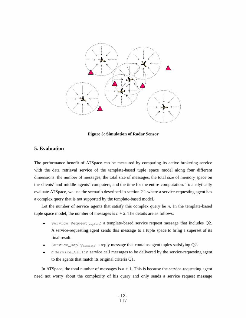
Figure 5: Simulation of Radar Sensor

5. Evaluation

The performance benefit of ATSpace can be measured by comparing its active brokering service with the data retrieval service of the template-based tuple space model along four different dimensions: the number of messages, the total size of messages, the total size of memory space on the clients’ and middle agents’ computers, and the time for the entire computation. To analytically evaluate ATSpace, we use the scenario described in section 2.1 where a service-requesting agent has a complex query that is not supported by the template-based model.

Let the number of service agents that satisfy this complex query be n. In the template-based tuple space model, the number of messages is n + 2. The details are as follows:

Service_Requesttemplate: a template-based service request message that includes Q2.

A service-requesting agent sends this message to a tuple space to bring a superset of its final result.

Service_Replytemplate: a reply message that contains agent tuples satisfying Q2. n Service_Call: n service call messages to be delivered by the service-requesting agent

to the agents that match its original criteria Q1.

In ATSpace, the total number of messages is n + 1. This is because the service-requesting agent need not worry about the complexity of his query and only sends a service request message

- 12 - 117

(Service_RquestATSpace) to an atSpace. This message contains the code that represents its criteria

along with a service call message which should be sent the agents that satisfy the criteria. The last n messages have the same explanation as in the template based model except that the sender is the atSpace instead of the service-requesting agent.

While the difference in the number of messages delivered in the two approaches is comparatively small, the difference in the total size of these messages may be huge. Specifically, the difference in bandwidth consumption (BD: Bandwidth Difference) between the template-based model and the ATSpace one is given by the following equation:

BD = [size(Service_Requesttemplate) – size(Service_RequestATSpace) ] + size(Service_Replytemplate)

In general the ATSpace service request message is larger, as it has the matching code, and thus the first component is negative. As such, ATSpace will only result in a bandwidth saving if the increase in the size of its service request message is smaller than the size of the service reply message in the template-based approach. This is likely to be true if the original query (Q1) is complex such that turning it into a simpler one (Q2) to retrieve a superset of the result would incur a great semantic loss and as such would retrieve a lot of the tuples from the template-based tuple space manager.

The amounts of the storage space used on the client agent’s and middle agent’s computers are similar in both cases. In the general tuple space, a copy of the tuples exists in the client agent, and an atSpace also requires a copy of the data for the mobile object to address the data integrity issue. However, if a creator of an atSpace opts to use a shallow copy of the data, the size of such a copy in the atSpace is much less than that of the copy in the client agent.

The difference in computation times of the entire operation in the two models depends on two factors: the time for sending messages and the time for evaluating queries on tuples. As we explained before, ATSpace will usually reduce the total size of messages so that the time for sending messages is in favor of ATSpace. Moreover, the tuples in the ATSpace are only inspected once by the mobile object sent by the service-requesting agent. However, in the template-based approach, some tuples are inspected twice: first, in order to evaluate Q2, the template-based tuple space manager needs to inspect all the tuples that it has, and second, the service-requesting agent inspects these tuples that satisfy Q2 to retain the tuples that also satisfy Q1. If Q1 is complex then Q2 may not filter tuples properly. Therefore, even though the time to evaluate Q2 against the entire tuples in the tuple space is smaller than the time needed to evaluate them by the mobile object, most

- 13 - 118

of the tuples on the tuple space manager may pass Q2 and be re-evaluated again by the service-requesting agent. This re-evaluation may have nearly the same complexity as running the mobile object code. Thus we can conclude that when the original query is complex and external communication cost is high, ATSpace will result in time saving.

Apart from the above analytical evaluation, we also evaluated the saving in computational time resulting from using the ATSpace in the UAV domain using the settings mentioned in section 4. Figure 6 shows the benefit of ATSpace compared to a general tuple space that provides the same semantic in the UAV simulation. In these experiments, UAVs use either active brokering service or data retrieval service to find their neighboring UAVs. In both cases, the middle agent includes information about locations of UAVs and targets. In case of the active brokering service, UAVs send mobile objects to the middle agent while UAVs using data retrieval service send tuple templates. The simulation time for each run is around 40 minutes, and the wall clock time depends on the number of agents. When the number of agents is small, the difference between the two approaches is not significant. However, as the number of agents is increased, the difference becomes large.

0

100

200

300

400

500

600

200 400 600 800 1000

Number of Agents

Wal

l Clo

ck T

ime

(Min

)

ATSpaceTuple Space

Figure 6: Wall Clock Time for ATSpace and Tuple Space

Figure 7 shows the number of messages, and Figure 8 shows the total size of messages in the two approaches, although the number of messages required is similar in both cases. However, a general tuple space requires more data movement than ATSpace, the shapes of these two lines in Figure 8 is similar to those in Figure 6. Therefore, we can hypothesize that there are strong

- 14 - 119

relationship between the total size of messages and the wall clock time of simulations.

0

5

10

15

20

25

200 400 600 800 1000

Number of Agents

Num

ber o

f Mes

sage

(M)

ATSpaceTuple Space

Figure 7: The Number of Messages for ATSpace and Tuple Space

0

5000

10000

15000

20000

25000

30000

35000

200 400 600 800 1000

Number of Agents

Tota

l Num

ber o

f Mes

sage

s (M

Byt

es)

ATSpaceTuple Space

Figure 8: The Total Size of Messages for ATSpace and Tuple Space

6. Related Work

- 15 - 120

In this section we compare our ATSpace model with three related approaches: Other tuple space models, the Java Applet model, and finally mobile agents.

6.1 ATSpace Vs. Other Tuple Space Models Our work is related to Linda [Car89, Gel85] and its variants, such as JavaSpaces and TSpaces [Leh99, Sun03]. In these models, processes communicate with other processes through a shared common space called a blackboard or a tuple space without considering references or names of other processes [Car89, Pfl98]. This approach was used in several agent frameworks, for example OAA and EMAF [Bae95, Mar97]. However, these models support only primitive features for anonymous communication among processes or agents.

From the middle agent perspective, Directory Facilitator in the FIPA platform and Broker Agent in InfoSleuth are related to our research [Fip02, Jac96]. However, these systems do not support customizable matching algorithm.

Some work has been done to extend the matching capability in the tuple space model. Berlinda allows a concrete entry class to extend the matching function [Tol97], and TS uses policy closures in

a Scheme-like language to customize the behavior of tuple spaces [Jag91]. However, these approaches do not allow the matching function to be changed during execution. OpenSpaces provides a mechanism to change matching polices during execution [Duc00]. OpenSpaces groups entries in its space into classes and allows each class to have its individual matching algorithm. A manager for each class of entries can change the matching algorithm during execution. All agents that use entries under a given class are affected by any change to its matching algorithm. This is in contrast to ATSpace where each agent can supply its own matching algorithm without affecting other agents. Another difference between OpenSpaces and ATSpace is that the former requires a registration step before putting a new matching algorithm into action. Object Space allows distributed applications implemented in the C++ programming language to use a matching function in its template [Pol93]. This matching function is used to check whether an object tuple in the space is matched with the tuple template given in rd and in operators. However in ATSpace, the client

agent supplied mobile objects can have a global overview of the tuples stored in the shared space, and hence, it can support global search behavior rather than one tuple based matching behavior supported in Object Space. For example, using ATSpace a client agent can find the best ten service agents according to its criteria whereas this behavior cannot be achieved in Object Space.

TuCSoN and MARS provide programmable coordination mechanisms for agents through Linda-

- 16 - 121

like tuple spaces to extend the expressive power of tuple spaces [Cab00, Omi98]. However, they differ in the way they approach the expressiveness problem; while TuCSoN and MARS use reactive tuples to extend the expressive power of tuple spaces, ATSpace uses mobile objects to support search algorithms defined by client agents. A reactive tuple handles a certain type of tuples and affects various clients, whereas a mobile object handles various types of tuples and affects only its creator agent. Also, these approaches do not provide an execution environment for client agents. Therefore, these may be considered as orthogonal approaches and can be combined with our approach.

6.2 The ATSpace Model vs. the Applet Model ATSpace allows the movement of a mobile object to the ATSpace manager, and thus it can be confused with the Applet model. However, a mobile object in ATSpace quite differs from a Java applet: a mobile object moves from a client computer to a server computer while a Java applet moves from a server computer to a client computer. Also, the migration of a mobile object is initiated by its owner agent on the client computer, but that of a Java applet is initiated by the request of a client Web browser. Another difference is that a mobile object receives a method call from an atSpace agent after its migration, but a Java applet receives parameters and does not receive any method call from processes on the same computer.

6.3 Mobile Objects vs. Mobile Agents A mobile object in ATSpace may be considered as a mobile agent because it moves from a client computer to a server computer. However, the behavior of a mobile object differs from that of a mobile agent. First of all, the behavior of objects in general can be compared with that of agents as follows:

An object is passive while an agent is active, i.e., a mobile object does not initiate activity. An object does not have the autonomy that an agent has: a mobile object executes its method

whenever it is called, but a mobile agent may ignore a request received from another agent. An object does not have a universal name to communicate with other remote objects; therefore,

a mobile object cannot access a method on the remote object, but a mobile agent can communicate with agents on other computers. However, note that some object-based middleware may provide such functionality: e.g., objects in CORBA or DCOM [Vin97, Tha99]

- 17 - 122

may refer remote objects. The method interface of an object is precisely predefined, and this interface is directly used by

a calling object.5 On the other hand, an agent may use a general communication channel to receive messages. Such messages require marshaling and unmarshaling, and have to be interpreted by receiver agents to activate the corresponding methods.

While an object is executed as a part of a processor or a thread, an agent is executed as an independent entity; mobile objects may share references to data, but mobile agents do not.

An object may use the reference passing in a method call, but an agent uses the value passing; when the size of parameters for a method call is large, passing the reference to local data is more efficient than passing a message, because the value passing requires a deep copy of data.

Besides the features of objects, we impose additional constraints on mobile objects in ATSpace:

A mobile object can neither receive a message from an agent nor send a message to an agent. After a mobile object finishes its operation, the mobile object is destroyed by its current middle

agent; a mobile object is used exactly once. A mobile object migrates only once; it is prevented from moving again. The identity of the creator of a mobile object is separated from the code of the mobile agent.

Therefore, a middle agent cannot send a mobile object to another middle agent with the identity of the original creator of the object. Thus, even if the code of a mobile object is modified by a malicious server program, the object cannot adversely affect its creator. Moreover, since a mobile object cannot send a message to another agent, a mobile object is more secure than a mobile agent.6 However, a mobile object raises the same security issues for the server side.

In summary, a mobile object loses some of the flexibility of a mobile agent, but this loss is compensated by increased computational efficiency and security.

7. Conclusion and Future Work

In this technical report we presented ATSpace, Active Tuple Space, which works as a common shared space to exchange data among agents, a middle agent to support application-oriented

5 Methods of a Java object can be detected with the Java reflection mechanism. Therefore, the predefined interface is not necessary to activate a method of a Java object. 6 [Gre98] describes security issues of mobile agents in detail.

- 18 - 123

brokering and matchmaking services, and an execution environment for mobile objects utilizing data on its space. Our experiments with UAV surveillance simulations show that the model may be effective in reducing coordination costs. We have described some security threats that arise when using mobile objects for agent coordination, along with some mechanisms we use to mitigate them. We are currently incorporating memory use restrictions into the architecture and considering mechanisms to address denial of service attacks that may be caused by flooding the network [Shi02]. We also plan to extent ATSpace to support multiple tuple spaces distributed across the Internet (a feature that some Linda-like tuple spaces [Omi98, Sny02] already support).

Acknowledgements This research is sponsored by the Defense Advanced Research Projects Agency under contract

number F30602-00-2-0586.

References [Agh93] G. Agha and C.J. Callsen, “ActorSpaces: An Open Distributed Programming Paradigm,”

Proceedings of the 4th ACM Symposium on Principles & Practice of Parallel Programming, pp. 23-32, May 1993.

[Bae95] S. Baeg, S. Park, J. Choi, M. Jang, and Y. Lim, “Cooperation in Multiagent Systems,” Intelligent Computer Communications (ICC ‘95), Cluj-Napoca, Romania, pp. 1-12, June 1995.

[Cab00] G. Cabri, L. Leonardi, F. Zambonelli, “MARS: a Programmable Coordination Architecture for Mobile Agents,” IEEE Computing, Vol. 4, No. 4, pp. 26-35, 2000.

[Cal94] C. Callsen and G. Agha, “Open Heterogeneous Computing in ActorSpace,” Journal of Parallel and Distributed Computing, Vol. 21, No. 3, pp. 289-300, 1994.

[Car89] N. Carreiro, and D. Gelernter, “Linda in context,” Communications of the ACM, Vol. 32, No. 4, pp. 444-458, 1989.

[Dav83] R. Davis and R.G. Smith, “Negotiation as a Metaphor for Distributed Problem Solving,” Artificial Intelligence, Vol. 20, No. 1, pp. 63-109, January 1983.

[Dec96] K. Decker, M. Williamson, and K. Sycara, “Matchmaking and Brokering,” Proceedings of the Second International Conference on Multi-Agent Systems (ICMAS-96), Kyoto, Japan, December, 1996.

- 19 - 124

[Duc00] S. Ducasse, T. Hofmann, and O. Nierstrasz, “OpenSpaces: An Object-Oriented Framework for Reconfigurable Coordination Spaces,” In A. Porto and G.C. Roman, (Eds.), Coordination Language and Models, LNCS 1906, Limassol, Cyprus, pp. 1-19, September 2000.

[Fip02] Foundation for Intelligent Physical Agents, SC00023J: FIPA Agent Management Specification, December 2002. http://www.fipa.org/specs/fipa00023/

[Gel85] D. Gelernter, “Generative Communication in Linda,” ACM Transactions on Programming Language and Systems, Vol. 7, No. 1, pp. 80-112, January 1985.

[Gre98] M.S. Greenberg, J.C. Byington, and D.G. Harper, “Mobile Agents and Security,” IEEE Communications Magazine, Vol. 36, No. 7, pp. 76-85, July 1998.

[Jac96] N. Jacobs and R. Shea, “The Role of Java in InfoSleuth: Agent-based Exploitation of Heterogeneous Information Resources,” Proceedings of Intranet-96 Java Developers Conference, April 1996.

[Jag91] S. Jagannathan, “Customization of First-Class Tuple-Spaces in a Higher-Order Language,” Proceedings of the Conference on Parallel Architectures and Languages - Vol. 2, LNCS 506, Springer-Verlag, pp. 254-276, 1991.

[Jan03] M. Jang, S. Reddy, P. Tosic, L. Chen, and G. Agha. “An Actor-based Simulation for Studying UAV Coordination,” Proceedings of the 15th European Simulation Symposium (ESS 2003), pp. 593-601, October 2003

[Leh99] T.J. Lehman, S.W. McLaughry, and P. Wyckoff, “TSpaces: The Next Wave,” Proceedings of the 32nd Hawaii International Conference on System Sciences (HICSS-32), January 1999.

[Mar97] D.L. Martin, H. Oohama, D. Moran, and A. Cheyer, “Information Brokering in an Agent Architecture,” Proceedings of the Second International Conference on the Practical Application of Intelligent Agents and Multi-Agent Technology, London, pp. 467-489, April 1997.

[Omi98] A. Omicini and F. Zambonelli, “TuCSoN: a Coordination Model for Mobile Information Agents,” Proceedings of the 1st Workshop on Innovative Internet Information Systems, Pisa, Italy, June 1998.

[Pfl98] K. Pfleger and B. Hayes-Roth, An Introduction to Blackboard-Style Systems Organization, KSL Technical Report KSL-98-03, Stanford Knowledge Systems Laboratory, January 1998.

[Pol93] A. Polze, “Using the Object Space: a Distributed Parallel make,” Proceedings of the 4th

- 20 - 125

IEEE Workshop on Future Trends of Distributed Computing Systems, Lisbon, pp. 234-239, September 1993.

[Shi02] C. Shields, “What do we mean by Network Denial of Service?,” Proceedings of the 2002 IEEE Workshop on Information Assurance and Security, United States Military Academy, West Point, NY, pp. 17-19, June 2002.

[Sny02] J. Snyder and R. Menezes, “Using Logical Operators as an Extended Coordination Mechanism in Linda,” In F. Arbab and C. Talcott (Eds.), Coordination 2002, LNCS 2315, Springer-Verlag, Berlin Heidelberg, pp. 317-331, 2002.

[Sun03] Sun Microsystems, JavaSpacesTM Service Specification, Ver. 2.0, June 2003. http://java.sun.com/products/jini/specs

[Syc97] K. Sycara, K. Decker, and M. Williamson, “Middle-Agents for the Internet,” Proceedings of the 15th Joint Conference on Artificial Intelligences (IJCAI-97), pp. 578-583, 1997.

[Tha99] T.L. Thai, Learning DCOM, O’Reilly & Associates, 1999. [Tol97] R. Tolksdorf, “Berlinda: An Object-oriented Platform for Implementing Coordination

Language in Java,” Proceedings of COORDINATION ’97 (Coordination Languages and Models), LNCS 1282, Pringer-Verlag, pp. 430-433, 1997.

[Vin97] S. Vinoski, “CORBA: Integrating Diverse Applications within Distributed Heterogeneous Environments,” IEEE Communications, Vol. 14, No. 2, pp. 46-55, Feb 1997.

- 21 - 126

Appendix A: Mobile Object for Local Broadcast Communication public class CommunicationMobileObject implements MobileObject protected final static double BROADCAST_RANGE = 50000.0; // range for broadcast communication private Point m_poPosition; // location of the current location of a UAV /** * Creates a mobile object with the location of the caller UAV agent. */ public CommunicationMobileObject(Point p_point) m_poPosition = p_point; /** * Defines the 'find' method. */ public AgentName[] find(AgentTuple[] p_ataTuples) double dEWDistance = m_poPosition.getX(); double dNSDistance = m_poPosition.getY(); LinkedList llReceivers = new LinkedList(); for (int i=0; i<p_ataTuples.length; i++) if (p_ataTuples[i].sizeOfElements() == 1) Object objItem = p_ataTuples[i].getElement(0); try // // check the type of a field of a tuple. // if ( (Class.forName("app.task.uav.Point").isInstance(objItem)) ) Point poObject = (Point) objItem; double dDistance = Math.sqrt( Math.pow((poObject.getX() - dEWDistance), 2.0) + Math.pow((poObject.getY() - dNSDistance), 2.0) ); // // compute the distance between the caller UAV and another. // if ( dDistance <= BROADCAST_RANGE) llReceivers.add(p_ataTuples[i].getAgentName()); catch (ClassNotFoundException e) System.err.println(">> Investigator.search: " + e); // // return the names of neighboring UAV agents. // AgentName anaReceivers[] = new AgentName[llReceivers.size()]; llReceivers.toArray(anaReceivers); return anaReceivers;

- 22 - 127

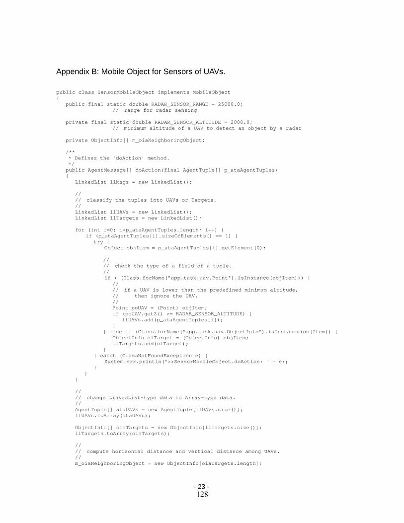
Appendix B: Mobile Object for Sensors of UAVs. public class SensorMobileObject implements MobileObject public final static double RADAR_SENSOR_RANGE = 25000.0; // range for radar sensing private final static double RADAR_SENSOR_ALTITUDE = 2000.0; // minimum altitude of a UAV to detect an object by a radar private ObjectInfo[] m_oiaNeighboringObject; /** * Defines the 'doAction' method. */ public AgentMessage[] doAction(final AgentTuple[] p_ataAgentTuples) LinkedList llMsgs = new LinkedList(); // // classify the tuples into UAVs or Targets. // LinkedList llUAVs = new LinkedList(); LinkedList llTargets = new LinkedList(); for (int i=0; i<p_ataAgentTuples.length; i++) if (p_ataAgentTuples[i].sizeOfElements() == 1) try Object objItem = p_ataAgentTuples[i].getElement(0); // // check the type of a field of a tuple. // if ( (Class.forName("app.task.uav.Point").isInstance(objItem))) // // if a UAV is lower than the predefined minimum altitude, // then ignore the UAV. // Point poUAV = (Point) objItem; if (poUAV.getZ() >= RADAR_SENSOR_ALTITUDE) llUAVs.add(p_ataAgentTuples[i]); else if (Class.forName("app.task.uav.ObjectInfo").isInstance(objItem)) ObjectInfo oiTarget = (ObjectInfo) objItem; llTargets.add(oiTarget); catch (ClassNotFoundException e) System.err.println(">>SensorMobileObject.doAction: " + e); // // change LinkedList-type data to Array-type data. // AgentTuple[] ataUAVs = new AgentTuple[llUAVs.size()]; llUAVs.toArray(ataUAVs); ObjectInfo[] oiaTargets = new ObjectInfo[llTargets.size()]; llTargets.toArray(oiaTargets); // // compute horizontal distance and vertical distance among UAVs. // m_oiaNeighboringObject = new ObjectInfo[oiaTargets.length];

- 23 - 128

for (int i=0; i<ataUAVs.length; i++) // // collect neighboring objects, such as targets. // int iNumNeighboringObjects = 0; Point pointUAV = (Point) ataUAVs[i].getElement(0); double dX = pointUAV.getX(); double dY = pointUAV.getY(); for (int j=0; j<oiaTargets.length; j++) double dDistance = java.lang.Math.sqrt( Math.pow(dX - oiaTargets[j].getEWDistance(), 2.0) + Math.pow(dY - oiaTargets[j].getNSDistance(), 2.0) ); if ( (i != j) && (dDistance < RADAR_SENSOR_RANGE) ) oiaTargets[j].setHDistance(dDistance); oiaTargets[j].setVDistance(0); m_oiaNeighboringObject[iNumNeighboringObjects++] = oiaTargets[j]; // // if there are more than one neighboring objects, // then create a message to send information about them to the UAV. // if (iNumNeighboringObjects > 0) ObjectInfo[] oiaObjectDetected = new ObjectInfo[iNumNeighboringObjects]; System.arraycopy(m_oiaNeighboringObject, 0, oiaObjectDetected, 0, iNumNeighboringObjects); Object[] objaArgs = oiaObjectDetected ; llMsgs.add(createAgentMessage(ataUAVs[i].getAgentName(), "alarm", objaArgs)); // // return agent messages to ATSpace. // AgentMessage anaMsgs[] = new AgentName[llMsgs.size()]; llReceivers.toArray(anaMsgs); return anaMsgs;

- 24 - 129

A Perspective on the Future of Massively ParallelComputing:

Fine-Grain vs. Coarse-Grain Parallel Models

Comparison & Contrast

Predrag T. TosicOpen Systems Laboratory, Department of Computer Science,

University of Illinois at Urbana Champaign (UIUC)201 N. Goodwin, Urbana, IL 61801 USA

Email: p-tosic@cs.uiuc.edu Fax: 217 - 333 - 9386

ABSTRACT "!#%$'&(&)*)+)',.-/0$21435&3768-9 :;=<2>;!?'@ABC .>;BCD@AE' F0!#;%:; ; GIH> ": KJL;!4E M @NE'. ;O@AP P<Q=E;E2= ABR4 ST;OE U ><'> VC> @NWEQ<WX? J4Y;!R E @Z =@NE[:'EQ!*@A \!"\ REE2;F@NE'G]^&_._.6#`+)Vab$'&(&)#)+)c <B ,.-9 9Q+,3868-9 6#_.3F/N-d+)V_Ce

&(376 fP,68&)L9Q+14(&)\9Q+38gY-(.h_i7jbklklm[no p,+)*) 14)&(D&1435-/N&3q&iqrCjon\ :A<Q>E@A Js>D@= 'M7E2t ='Mu4 @AJ;R)+&(96*9v\ D,.-/0$2)w+xbda9Q&/C67,_. EQ:;J;Gy0[XU:; Jz A<Q\:'XU W < 0@N4'M!@= :;JLE @AE'" c YC@A J\E2!# @N;. JLST;I!#;@|B@= \ @N~WE 4 <'z@NE'. o@AGU@NE ? O; BcXC?E 4@AE'

PJN :;W<Qb<U<;JNWYXWN0<VU<J GFN<VJ:Oo b'M5:;cM!OEE2B\ sE2w c ': . L!OEMEQA@= :;JE @AE'P!QW!#' XU<QO< ^Ct M7 sB\E I@N4 \ D\: ;F@CE4F V\KXUB<'J4@NTXW.D OOKXUz@= ?E ;@NcO<LE @NE'c!2w PF \ J\4RG"@NE % \'M b ^!#>!# @A;. E' O;!W: ;N@N4N O J>E B'Mw FJ4 c > = >'O <2_.37(1,3714(&) .149Q,3768-9Q&)":;G^b!# @A;. UM=<QqXUlt M7 BbE 0@N4 \0Bw ~?; M7; \E BI R l@N\@AE2B. Wu'E2 ': . W!IF;J'E2M T@A V:JNE T@NE'U< b;=BE ;@N?BRG

Permission to make digital or hard copies of all or part of this work forpersonal or classroom use is granted without fee provided that copies arenot made or distributed for profit or commercial advantage and that copiesbear this notice and the full citation on the first page. To copy otherwise, torepublish, to post on servers or to redistribute to lists, requires prior specificpermission and/or a fee.CF’04, April 14–16, 2004, Ischia, Italy.Copyright 2004 ACM 1-58113-741-9/04/0004 ... 5.00.

WWXWA;@N<!T@A 4YNW PE @AQ;E'T 0 A!#@;\@N4L :;N 'J ^Ou'BoE BM TR bXW ?!*B?;L;?@A@A JL :;P\P!# <P!#'P;!4E 4 FB<'@NE'G

Categories and Subject DescriptorsHG o'%4[Q5q4;BJN b4B:;JQ'G 'G ¡P¢2£T¤#¥A¦b§m[¤w£TR5o¨Yw CH0 J4N ©H0'@A . U¨G;G ªU¨G;G « U¨G 'G « ¬L¢%¥'mm¢2j=¥­¤w®'¥®¯%'m7F¨Uw LH0%0'M %02°c TH0 ±<'J'B@A ²UG;G « r¢Q³s´c¯R®®¤#¢Q¶µT·¸j=µm®[ ¥®¦b4¹"¤#¥;4m5\;!?¨Y;@OME'.

General Terms±;Rz?BJ

KeywordsE R;@NE'. o@N4@A :;JAE T@AE'@CE@AE'R<'^J4@NT MXU4' ';@A .

1. INTRODUCTION AND BACKGROUNDON PARALLEL MODELS

²IT'º= =$'&(&)*)+) 6#_./»@AE' :;F<2l@A B<4BW!I R2 XU" 0 @AO P. !#@AE'!wKX? A 'X? M;o ;l b B= J¼½;G|E@= BJ:4\!#?<2O!#i8E!# <J;;@= :;[n%E BM @¾s<Q!wKX? N s 'X A F<2RI sW:BM5C=!#PJ;YPEQ!*@A RE Bw E@A J=!#;?,.-/0$21435&3768-92&)"_5$+.+dG @AJ;W ^B. ¿!* @N. L@AV. ;W@OM

E2;l<;JbFw XW!EJ4zÀ4-g&_.3F z@AE'XWV© lVJ4;w Y@NE'. RGb@N. <JoW:;BJz R F.JzMUEQG0b E'ME ^^!#b;4VJXÁ@NE'. @A[XU:;'?YXU;BAXWWCUu4F.MU ©XWJl@No!#B+`-)V143867-9Â ^bX?MB. <¿E l@NE'z 'X? |

130

;b&)-9T+ =;zl<Qb <NED. zu'E2w ? z@NE'NE2!#@= z@NE[:;@N!#;O;O N lOqX?ei7 Oz@N;BnG©@A: X UP!#;[XFU4!#4< JA@NLu'C.;G5 "<Q \ "qXUW@A L.; :4

!#; Y 'X 0:;T<2bB. FLu'E2;'Mw T[X?ob. T;@NE'?EQ[:;YLE b!:4M ' c :;?<2zi8#n%UOEQX?BM5w X©@NE[:;M@AY= U = ºU!F< F@AM5@NEQ;W. WXAQ i8#nR@A %@AE:@A;"FYLJ'YE2 HL²07G"¿Ab@= A@NF :;=O<2> i*J;n;W!* @N. 2 XWP!TEJ4P@NEJC PW@OMI Pt VU R!#;X:;; J\<2U .RGclE2t J;Ue z!Wz:;BM5 ºN;!Wz< M=o;@NE2;OCow XO!@AM5:;< EEl!4 @ @A o lE2^!# @N;. 0@AVAlBoX¾@= i7 [X zA;F l.E2nL A< N;=@NEQ;<2G² ;YB. XWV=@NEQ;UºU EE .;P M7 L o<QJR' ;@ @N QST >!# @A. YEEC.© cG Gcy04<2 C'MB. ;KJ^EEI<2@AA!?'@NF@NEQB. I :;A YE2<qJ^;!?!#YE;J' Y <KJ^!C M7:'F ^L<2 :';<Q;@N\ b@= [B;0MGcqb !%NJ4=U R?U !# @N;. %w X¸!cEJ4WMPFEE!#@ EQw "M :'qJ l; E;E ; A!* F ^=E2!PM? \@NE0 NE2[XUBM7w X @AE:@A;E4?E2W@AEVJ= W;4A&;dA6*9f96*3814/CG5?@AE2B. UC@AE º0 ?L@A E;J'

@N C.149Qd&/A+93q&) !#bE2;N!W JE Bw zi8NO!#'[n@NE'O 'X? b.MJL@NE@N. RG5F\@A@Nw \;O sE AFºF;!I@N B 0@A 4^¨U°0b AXUW =@N@N;A!* B?<'bJ©XWV\@N. ?@AE2o<J=\w X!IE;J'Gcy0[XU:;F@AE2B. ;\lB. D D EE N \A@AEM !qcG Gt =E2C!F&9ah6#92ds-BA_.6v92&)EE M; ;s¿&9 azh6#9Qd^-Kb&N$ Àa_.68,.&)_.a_3K+/ -(A/A+d6*14/ i8@OME'. %0BX[n X% EEJo= ;Jz;: <!#'W@AE'PEQ:;0!TXE!#;VJA!#M!#"P!#;@A FE0@A ."@Nw !'!#'L@= JA<QL!#@ UE ?;UE?;GcqoE B'Mw ;0!# @A. EJ' 2@AIXW :; <JO :;@N?E!#A@NE ;IO@NE'c.!!*'4:;A!K;!*u @NE;X.;;PFW@N Wi8;PqJ'E2P!Q .n = 8YO:;e!Wz@NE'NsA :;l¨?°0N @A@A 0XUC :4XW@ :;BJ ':;;L!;\. R;@NE'G ! RFE;J' "@N@NEQz<JoF XWW!I

XU\t zFt VEQ!I!#;@A zEE ; ;oA :;Y@AE!#N C!* BM5 .@NE G"?c NAU\. BJC\@NE'\@N4'MO!O&_b/N&_._.6#`+C$'&(&)#)w+)V6#_./ K&3C&)*)U)+`+)V_C&92d6#9$'&(3867,14)&(6#938À+bÀ'&(dgP&(+D&_C$'-__.6)+ AU N@= :;o \&3714(+ E2@NGOq^\4BF!#;\s@A :;JE BM R@N4[XU:;;\oW@A?Wu'E JFL?E @NE'L@N4P c@OME@N. ? W O44z "!I@Nw qJAXWo4[XR4u'F' =A!#<2W:'XU Ai8E2<[n0!#B=+`-)V143867-9Q&(a¾ ': @NF b

XUM74[X; FEEG q|E B 0s;i8C E > !#'[n\. =!?@NE' Ab@NE2; @AN;A:4;!R: <@= :;JNE Q!#@= =E:4 b@Nw F!R!#'Gc?E E2?? @A? M@NE'cL ?@NUEQ<U JEON E!YVJ=(+`-)V143867-9Q&(as@A! E 4@NE'; !"\X|E R@AE'N!#G

1.1 Limits of the “von-Neumannian”sequential models

O @NE'\R" o[XWs 7`-9F+1 /N&99,.-/0$ 1'3q+(&(,À6#3q+,381'(+"!FP< AN!#[XLqXUE@N i8#nAsz > oEJ' \ oXU\ o; E !#@ X . > ¿E @Ao i8@N@ABJnF XWsD@AE'. |u4'pi8EMi8nn" i8#n oE\u''F< OBi8EQ ;.n0N F =@NR7G GRw VJ;GC ;JE Bw E BW :;\<Q@A \!#;@ W< \ %;@OME'b@N47G|² =u @NE?EEQD=;!0lX J'!u'E>6#9 _.38(1,3768-9q)w+`+)"$'&(&)#)+) 6*_/ $#&%('( :;©© ;M5E@A .G*)QC!# @A. I;<2KXUE> B U!#Al@ABAE B,+[ @A RGLqE B ci8wn@AE0 . A 0= :;!#@ XW\WoNXFV0WEDi7 l< .n 0 ;VJzbb AE2=; W lEQ!IXW Ci8wnU@NE? \< \; 'MA!*OF . O!#;@ N\ . OO ' '<QJb@A0<2t?WC QB b@N4w qJA!RE4' A0EQ<VKJN!Ru'E;VMF !#@NA'M5:;2E @.-4'Mw JF'u''N 0@NPM% C OC; ?. L@AWt [XU:;?@N @N;;?!%@AGl@A: zl!0: ;i8 wnCE VMY@AO O lX J;![:;;@Nlb@N. F;!ABB© O l@A~w CDCR >'Js :;PF0u'BEY:4GI@A@ABJN VKJN@NL. R0/O /.ªGqE Bw ?XU^@AE º s&9a w

@NE':;0@= @N4\< |zBXW0 W!c N;\E4A@N0 E <F!u''JAW;= ? \@AW Y@Nt 0E2R4[XU:;!* '?:;; J=4@N=C0< 0XWVb:;BM5@N@A F N@A?@AEuO EE P OEQ!*BM@A L4@N;1Gcy0<O;@NE'Y ? :;@CELE4A@A?X? ºzO<QF O@= ?!VKJb@= ;J=J; W G4@A?!T!# @A. 4B P JO

u40 \!#;[XW M >XW C< bE@A>@A :;VJsE YJ4M

@N<2\<32+y0[XU:;4/,/ª'GF 0/.«G- ² B?=^i865"°YnP =@Nw .4 <2MJ;oUE2LRG5?NUC. J;4 ?65°©@A JA'M <J@NE[:;l4;w 0@AE', =EQ!#@A <'Vc c!# @N;. JF[:;@NY?<2.4I@OM@NO!*@ZLqXUN!# @N. % @AE';G1 q ;Rl zs@= JD@AE2B. N;@NE'. E<@Nc P <2c?!QAJ;@C.O@A ;J=:;bbE 7 RoE Bw ' o<2L 'M JO@= EE2= b .XWV=@CEWEGy0[XU:; o 'JE2'0oo JEQ!*BM@A I D @Ao: ;\EQ!*@A A@A"E@= J?E2O;!2u4'R :;?<2O?;@N cV:'!#<Qz\4W!#@A :;LE @zG

131

M2y0[X© PST;E4W"4 P OEcEA @A@A:;I?@AE'. O \l32MQ I PY@A P@N"!Y@AE'. E2[XU

!lE @A? X b zl@NN[X@CC C<Q?; XWU@Ac@AI!2EQN PEQ!*@A 0@NA@AE N\W@N. oL4@A!"@NE <w R@N4i8G G" B'°c7" °QH°QHW*n2?X?|!#^ ;@NE ¸ Bs!NqX?

E!*JDSTOw C!WE U@N4GsbqX?w P!T@AU W< A;A!# @N;. JOST;U< E@N bW VW 4;J; ;JST;Gc?Wt BU Y W=Bw ~FE 2@AE'M%.s \@CVE4LEQ@AE'F sKXU<'OJ'B@Ne IXU?4[X©@lGcw P O@= s;E' Y. N=<'BF!UAB! /[G?lw 0 \Wf9Q+8v(&6*9Q+dF$'&(&)#)+)"/N-d +) _U L C< o,.-99T+,3768-9 6#_.3eE @ H25GUqX?EQ E<Q4[XOu @NEc! B4z!"t M7 lE @z':4ºG' W '@= . C %KXU44XWR<2\zz /4G©@A ;© @AE2B. ;^ Vt ; ¿^

!O>@Nbf9Q+8v(&6#9 B+d3» ,.-&(_+38v(&6#9( B+d3 E M@zGI²I; @AE'P0Pt :'GD; o 4w qJD!WE U@NE's N<2e!#MX? s 'X? s:;G ² zu @AEL zs!wKX? :;7L ¶lt M7 |:4; M5 |DM@AE2;i8G G;<4B.nGzb b EEEM lN!L 4 VKJ;U e!#zt MC ; M bE @zXoV?@AYCE QE @N@N E'@NºO@AE.4T l;B 0!#\G G H5(c5GW":;"XW J!c;C!P 4 VKJ;GLq RTXUC!#4>b;>!W w KJP ©@AE =t b:'G E @l%;JssAu4!Li7 < n@N4F!E @AE'z .Gpl;[:;0o¿!t M5 ©E @ i8>o 'X? [nO< ©;>BE ;@Á H25'X <J=; M5 E @ XUF@A "w %@CE2@C@NME'\ ^B<'^J'B@NMb;C \@C.!IF \XU <2Kt M7 ~ 2. 2G G2M<'s@N@N;BJ@CVE4LE2@NE'\ F@A J :;D :¸^!O !OE4GqDE Bw I<;J f9Q+8v(&6*9 B+d3O$'&(&)#)w+)Y/N-d+)V_ ! XUA !#W@A RT,.-99T+,3768-96*_3f9Q+8v(&6*9 B+d3F/N&__.6#`+) aW$'&(3&)#)w+)%/N-d;+) _.G; ©!\^.^!F ¿ V^!

@= :;JOE Q@= .;XW=E YWt BYKXU4M\sO <2[:; F@AE2B. ;F@AE \!#LR ;@NLw %z ;WMFy0[X el@CEzE4;A<2l;; º

o2MH0W0EP W ;4YY .b!Q@

?E@A JF!#4CUqX?u4\ .?@N4'Mo!#oE L;@NE'. R0 bJ¿ 0 DWKXUzBu@A~\ N ?KXUzBEB~\E @NE'E ;@NG?A N@A ;J@Nw ~o@N4. UG GY<'@N@NBJ>@CM7E4N@N4 L!* LB;@NXC^<2qX?~bC 'M7@A@NBJl@CME4; |i8EJ' J lXU VJ nbM<' D!o;@NE'D@NE'|J4@N N> c; z;N<'BJ'@<J\ F EE;E 0,.-/C/C14967,&3768-9A9Q+37gP-(.h[ F %XU @NEJ=!#?A Fd6#_.37(6143q+dA_.a_.3K+/C_.G

N :;LXWB ~O@A@ABJ 2M?y0[X ;;L^<2CN;Ez @AbST;\EM

Fi7 oEQ<J=@NEQ;!".l O@A V:JE R@AE'NBJ'B@bn2MUy0X FST;E40A@A@C C BM

LXWVo;F 2P A!QW@= A=.P!*W@N@A cJ'

Bcw c!2E '@N4IXWCcEQt E @A !# G ² u @NE> .>!A :' s ;z Ns: = @A@NBJ©@AXWzzE4N©s<QoJ>Ee Xll@A ¶i8EQ<J©JnCX JeST=E4M?@N@C WXWVo\ ?Y:'w O!#;@ XWVbbO ^@A@NBJ;GO4@Nw J;QN.O!; ;C@A' IL@N4XW?;@N@C i Bt2 <Jl @N2nBJ'.;0T lFXW@N@C <QA © O J4cO RGDbKXU C;!@AO!w>4 <JASTYYb b J'º4!wM!#;A @AAE @NcSTO@N4!#@= J z <2' GqlB=;!0=RYXU'zKXUs@= ew

!LE 0@AE'b@Ab@NE'b^ @NE'A>!0J; J e4 JG?zqXUw i8#nP;JbEl@CVE4UJ4@N\i* ?KJ'E J

:;Y @A@ABJL; I B IE nL i8#nb4JERF@N ;sE < ¶B<'

J4@N0i* Y WY@N@ABJOP YE [nG¿Y!# @A;. J\STI@= ;J\E2PqXU

w %!4E ;@N4" ? c@AI@NEQB. %!# G Y!4@|% \<QF " .FV:' E4;%@NE'. ; VJCEQX?!*8GcH0A ;PVSTY EE; .^<s@A :;JE UJ4@NC©<Qo< RP'M RA:;BJM5w M5ºWKXU4YPP;!T;@AE0E4OGcEQX??;!%E RBJ'B@AP XU^<2N<\^L< CE@ACXU^E@= Jl@!#@¾O@AEu; s ;E @A; ?<;J@A:;c!2 0:;BJC@AVC;@OME'. E2[XUGI?N 4 VKJ'~0!2c :;?! E @A"XU;!*U<2U <J\t "!4c. F@CER%KXU\B<'J4@ i8UOBw ~E #nP VGc²2Y RLKXUE B lu' @NE!Cw !C@A©DOR:4ºGcb 'M7@A@NBJD@CEM FP@A. M7E B<'FJ4@NXUY 2/N-d+)V_?-BU,.-&(_+8v(&6#9Q+dU$'&(&)#)+) 6#_./CWF " :;' W%3*À+C,.-9 9T+,3768-96#_.3Y/N-d+) _-Kf9Q+8v(&6#9Q+d$'&(&)#)+) 6*_/Cl ?XWT<Q\Bz0/4G

1.2 Tightly coupled multiprocessorsF<2zFz;!E %@NE'N@AW<;J

t %?cw '`-9 +14/N&9 9N&(,À6#3K+,3714(+XW b;OE4;L ^ b@A@NBJ;% ^@NC>i87G GR . E 2n<QKXUsOqX?GNy0[X L .Oz<QNuMz!"XUF A z@N\E32Y P " RKXU;<;:'%G PW :c:M

E4 OXWVN[XWNL2_À'&(+d. K-(v)-"&) =/A+/N-(aG0H0.< l0@N4 N e_À'&(+dz/A+/N-(al/N&,À6#9T+_.GAqsE B %E4MN@A@C bXel O:' ^ !#@ XWVOC\ o@A@NBJ;GOs<:';L.;OL \ sE\ L

[XV:' "@A@ABJ;GW4Q0RQF!wM

132

!#OE@N@NBJE X?D J<QbBE2;W@NE'? Y z ;@NE'CBJ'M@z\ N<2 O@N@AoQ VJo s3*À+ 1'_ PEFGby0c .E4ML4F\[Xs@AE'. s s Js FJc[XWR; @A@ABJ;<'PE4 N L@N@C XWz; :'w OF l<G?°c % < I 4 U zd6#_.38(6 143K+dL/A+/N-(a\/N& ,À6#9Q+_.G?KXU=@A0;'^ <2[:;C <2:'X?s bE~

<'s@N@NBJ@A" F \;!* \ >@CVM5EE .> D'MRGA ;JJ4<^: ;\ J@NCz \@NRGqE Bw C ?KJ4E F@A@NBJL@CE4;%t F .DE4;D ^zA< @A@ABJ;; \ P[XWR4 @A@ABJ;GP4 @A@NBJ!T .AE4 A<QcBY \ .W!Tw :;VJO@A º zº <@A ~z@A@ABJ;"E2<JXF[XE Bw !#M z@A@NBJb .JGY\P F@A@ABJ\ .I FP<'

@A@ABJ .o< 0E@N=;'MN <2[:; Uu' @NEc!"/C1') 376 $2(-,+_._-(E '@AE'MGCqs@CEL@A .%; \!PXL@A@ABJz L<'>i8o =<L!<2~n@AB ;!Qc:'Y NP@NEF @NME'J'B@ P RGI[:;IJF G GE'M'E'Oi8& nW:'L <;J %CEQ<'\ PE2 WBJ'@pi n " \!8 <2KXU\P 'MX? L bNi8!wKX? [nY EE oo 'X? F o\ @AL!#W TE4GCC@A@ABJ; º LO;!cO; IM

N. : ;Pw Vt P DB. u4;@N~\!A. E P@N4 A J^< E2;i8G G 0H0 )0*n0 @= JPAE @NcXWW!#M!#ODO Dt ;JST;OE ; 4NR4 :;W <W@AE MY!*U.149Q,3868-9Q&) 6#37a=8G GWX? J4UE QE? o''bLST@N4GP4@N;!%LM RzE @AMz,.-/C/C14967,&3768-9 7/A+d6#14/ ! @N@NBJe:4G¶M

<'o@A@NBJ;@N ;E OJ4@NM3*À+F92&3714(+C-BL/A+/N-(ab&;,,+_._©!#;@ :4Gc4!*@zMv(&9 14)&(6*38a b:BJs N@C<QF!U@AEOE

?:4Gcw :;J=@A R@C<QW!"E2[XU!#%E4M6#9 _37(1,3867-9^_37(+&/C_©:'Gc@= ;JTM0d;&3q&=_.38(.+&/C_ ;L:4Gc@A ;JToG² bu @NEW!Lo D;B @z

C DE4;> l@CM7E4@A Au''=. @AAO O YCEIJ;CST;E4Pu4'WWBYASTY . 'XU 6#9v)+ #9 _.38(1,3768-9]14)V386 $2)w+&3q& #B] @A7G] #B]| # @N4W \t z@Nw J;G?e ©@A ;J¸!# @N. C. ei*¿<2©'M

z!#@ @N\A@N. U;t 0!\E WEW.nY WW!I O;JEN@CVE4I :;?L[:;@A?Nc\ .:;+0+,386#`+W@A :;E @ RRJRCJ4@ E2!#@= Yo G>q© o! D@A@ABJ^@= .=@A@NE2;B. ;CE<@ [X|= .:;A_,.&)&"6#)V6#37a WF4@C<2W!IE40 bºb!?o >@A@NBJ[XFG^² O@N;=> @A@ABJN@AUB? bt ' !#Dl= = <2'.'?&(&)#)w+)&9Qd;-/W,.,+_._]s&;,À6#9T+_D Aw = A@A@NBJA < Y@N4qX?

.¸!*s LHWHWO B'°c5G ?D@NE'PJA :; 'JN: =0B<'@N@ABJ0E @N4R?<Qc@Ac w <I L% @N@ABJ;;E BGq^ O!PB<'^@A@ABJl@CMEVF\A D @A@C ;:' /A+__&v4+$'&_._.6#94v FE2O@NN!N@= [B; ;LMAXl!* =!L!#z =.BJ'B@A= l@A AN<2zE; @ o!#;@A J= l <2;'G

1.3 Loosely coupled distributed systemso@CEA EE; A'e©zE:4

< W;VJzX? Jz! .:4=E @ 'X :;8G H0bE2;<KJe=> :;^ D;VMe!0ST;=@NE'XWVeEQ<J>4VzMC .IE2 J4@NFGc s;c ;P@= ."XC ;MzKXUQ O WJz l;@N@C \ l4EQ XWVz .lGY¨Y J=LX?z<2\N z@N@N;BJb.o@AYMc@A:'LUsB o<~ 'V O .C:4 '@= .Li7 O C92-d+n"U/C14) 3768,.-/0$2143K+("@A' cI[XOE2E :4; @= JSTc!#@ ?!2c4GqNc!*c.N LMU;=;!R@NE'Y<Q <0!*b;R O@N@Ab!8 s/C68d;d4)w+gY&(.+ O<QE[:4RG F AqX?ob %F!wM!#;o;@NE' ¿ s@A@N@AX? z!* \J^ |B. s s~"ST\@= .s. z@CV@AE'\BJ'@Á \Xs= :' _+9Qd6*9vl&9Qdb(.+,+6#`[6#9vo/A+_._&v+_.G0?u'. C!c@AM. L@A J<2C. 4bEw N O <OEJ4 B. MU0C CJ'B@NWXWCST;\;@OME'o ¿<;JDg68d+3B&(+&>9Q+37gP-(.h[_zi*H00nGV@AE'OJ4@NC!W: OBC A o'M¿<J D@A@C ;KXU XW zA PF \X?N :;LBF;'D = 4XWl d6#_.38(6 143K+dA_a_.3q+/C_G±<'FJ'B@N :P:; 4 ': . I:"P@CM

E\@A GOO!? ': . OL "[:; 8Jo L<QGP?Jo F O@A u'< @AL VJ@N4t2 <4't <\ ou4< bJ= @N;? !#VJ;GIH0 UXWVN?@A .I :;@A ;JNEPVJNE N;4=<'AJ4M@NPJNE A AW=!#P4C W JN >G^y0[XU:;Io = XW< .4 X?7G^² B<'¿J4@No ^@C.¿ o©\ BE; @N~C z@CVE4U@A GY4;RJ =@C.@AA Az:!wJ Rc; 7I!#@= J <Q'GA<2 :4NN<2l@C©NEM. <?: AqJ'E2=!0=A!* = B<'zBJ'B@ O<Q\@C.o ? oz \!@N;VJ=ElE R . lO;RGq= 0!RB<'AJ'B@NWqJ;';@OM

Y!#;@A Qt b!" FB<'=J4@Z ? FMN!T:' @AE' Y E A<2AE;J'VM JN N JC!#@ N4 OA;<JO@A?BP!T \@N@C OKXUQY JF@NB. R @AB; 7 l!I OB<'J4@ !#^@NE'G\5R[XU:;RAL!#WEWEE2;2 WWz!c OB<'zJ4@B:NCX?? Co;EE2bu@AbbJ'ME@CVE4E2@NE'lzE:'VMU<NM0EEQV0u4@N4[XU:;4JOXWXW XUUI<2YU I!",.-&(_+38v(&6#9\$'&(&) )+)R/N-d+) _.G² ;@N\i8w #nY<'oJ4@N'G G" ¨ ±*" 5(5R5G

133

@C F[:;. qX?0 BM BW0!*l@CEJ'B@NXUF 'M JA;!wJ; @AC'!*[XWC@A BUW z. M2Y P;!4YJ'0qXU;Oi8

EQJ;'N@N. @z'G nM%@A@C ;O@N48;:'ºG;XWP@A@C

BJ'.;W J'.Mc\\<'z z N@A @AMc: W4 'M5 zMPFE: Jl lVKJoCi8\NqJ'E VJz :4

ST;zl zSTB~n @N. @No!#@AC=@= b\EQG5P@A JO<2W EEQ \FVO\;A @N;

oE ? ©B<'e Vzw O!0@N4<JO@AE[J'F;@N?@NJO!#@ E;J'U @A J;@AE'Y WE;J' 2BJ'B@AG?W 'M7@A@NBJO@CVME4" W386vÀ38)VaL,.-1$ )w+dE @= .G"H0Fu@Nu @NE\XUl<Q AE2@NE'WXWV:; " !Jo;E^¨?°0G??@CE;J'<Q B<' @N@N;BJl .T <2F:'XU L@AX LVJ;ERG OC@A@ABJlL'MJB<'R0X?s : ©;JEJ'B@zG q o;!J><'eJ4@NcXWzAJDz= @N@NBJz;! Jl;B2<'\ A E40 FXWsE2E Y:'C s J; D 'M;@N@NE' XWb <XWV> =@A ML?E bXR'. J FXU'M7XqXU;4XU :;BJb4JbEl<'z@NE'OJ4@zG

2. FINE-GRAIN PARALLEL MODELS0 VJ u'B©E L@AE'z<z<J4@A

^ D@C<Qb!\@N@A!# G¸H0@A@NM@As!# IA PEEQBqJs\ @NF!Y= M E @NE'" ;B'L!4 ?w :;VJ@A4@C<2P!Tw :;JOE2[XU!#2E4FG¿XUb sJ©E 'M7@A@NBJe@CE4;C z:;BJs;J^ED;!?VST@NE'i8<2nKBJ'@A©:4w ^ KXUQco:4 B4~XWE4. "Ew P P!* J@AEuT KJ4E Jz E <C;!149 6#`+(_&)c,.-/0$21435&3768-9D y W7GD>R@N^@NEJB. ©E U ;OM!* N oÀ'-g /N&9 a . B4~s ©<QBE'N~^ AJ>XU;© A sAXU7G GU = szE BM Y@NE'Gq© o!@CEIb4@C<2O!ST;E?? VJ=bL L!P + [ 1G oO RP:;e < YKXU. bX?'MXWOXU<B;VJ'~l <Q'= N@AE'i7 !4Y JFn \R@A W;P.BJ'@Ai8W0º <F<J4@NnYX?o A RT !#^:'B J@NEQ<%B. 4 GAOA@NM<QP!QE4;@A JC<2:;BJO@AE:;UN@A JC;u4Jo 4VL@AUbL @NU!"<JA?B. EJ4G¶qb?RWV: <l>< @= :;J©E MU;@NE'C@AO!b!#'o>oEEO!#;'W!%@NE'YL =M0EE E @A? F JoE[:'RQ[XU:;2<Jo: M\@NEuBJ'@AL E <O;!P!*@A ^E4 % !#zzz<Jb?EJ'2 \. A<'zJ'B@:0 ¶ WFu@NEEQVFXEQA;;JzE@CEF_.1 $+(,.-/0$ 1'3q+(_.G

q\I @NE'I u4 W@NP@N@A\!# !4u4oE c@NE'RXUOE2;\'LNE 146#) 3aFÀ14/N&9_ !> PW<2!Q0E:'YE ERGIq !"@= 'M7@= ;@NE'':4 TE4CM<2LU\¨?°0UE2;<VJb ;XWb@N04 T@N@N;BJI?;U@AE'IJ4@N ?& :'P =BE2E w ~OMU 2 0 'JbEQ;l' !#;o<2b@AE'. J:BJEQ[XU!#7c<'O !* Js@NEu BJ;GAH0@AzF" N!PJE@NE'NJ4@NF \E;J' " zA@NMI "W[X>@A J\P EQ0:;"<QU <0ST:;JBE =~GPqz \!I4VJo;ElB<'zJ4M@N;o R0@A JE<@Ao lXWXO@A 0LST;EO@A;?ST:;J=;@OM@C Q; O 4E2 R0b<2O <F @NEo;@N@N;=. AVJz z <VJ;Gy0[XU:;F lW@N@Ao!* 0;!I@A 'M5@A

E %@NE'NBJ'@A?lW<QF l<;JbXW XU@A Jz 0JlE !*@A E=J4M@NW oW ~=@= Gq!8 2@= ;Jz 0 ~b@AWo EEJlu JzCEE2;'Mo^EE~GC"o % < JLO@NLEB ^!#@A ;EoM:'i8\@NE'.n<J^ O FF[XW^?MP @AJ;R3*À+\À14/N&9 (&6#9 G0?VJOEAE @NE'PA<;JN'M

@A L< 4@A \< R@A:;" cVJE@NE'\ :li8#n o:;BJ^w N4@C<2F!Li8#n;VJ;i8#nL:;BJD@NEb< o!#@A ;DE4BM>?:'ºG9Q+14(-9 _G H0;J@AE'z @AEWtu'!#¿;!FoE'G ¿^z Ro o@A JO>=4@A >< ¿i7 ; +!R@=n' =:;o@N0'M7M5;oi8@N\[ + !Q@=n' JNE Ab \w :;VJN@A :;@AGb@AEu'qJ!?=4@A >< M\ >!?4%;!!#@= E4WV%R E <!M @ARw Ji7 \B. J"u':;VJ nT!#@cKXU?4@C<2 Ow ;\4@C<2!LBE4;~2 l z:;lw 4@C<2!BE4BM8M7E4?@A@C ;b~GO @A ;JlWJl!8 = 0!

F@= o< 0 l[X|JbF lEW!#@= MRG¿W@N!QW!# P@A JO<2W!#;R4 Y Y Y!# 4:;8F@= 'M5@A P@AE'c "X?7@N!C I!# ;!I^;@NE'~= L<Jl< b0@AE'Y ?U<o EEQ Y<Q ST!#@ G @= Jl QQ lXU !#@ ?[XD<@AlE2[XU!#7?@Al3A;@N;C<%LJX? B!#7% s. EQ\JE BM R@NE'324@A^ l!#;z[X¾ EE; s. l!#@

<J4M7Eo oE;J'M7EbEQE2:;? :;0@AM: L \!' ? %! <B 0;@N4~C W L<4!"L<U !#[X\G

2.1 Artificial Neural Networks<2XW D<!F[:;B:4X ;!\ Dw b!LXW o

<2N:'XUD B@= :;JE @A~o C NVJE<;J©l= lM@NlE2t J;?<;J<VMJ;G=?N@N4F N< s;^A b F;:'w ;L ; L @Nb A:;BJzw ;4@OM<2\!:BJ@AEBE4~o@= JzJ'^E c;@OME'b o @A w <W@N;<W@NJAN >EQ<J:;>@A=@NE'. ; VJE2[XU!# ew E @N4A< u4

134

< 04;w Q:;b0@A o =: UX? J4GE @N4WXW@NE'. ; %EQ[XU00< NN;:4KJO NJ4;E2 A @N;0E4? 0!w= ^,.-9 9Q+,3868-9 6#_.3c/N-d+)V_c\ Ai H2*nG° ECo<QBN4[Xe ©@AC©w C;!,.-9

9T+,3768-96*_3/N-d+)V_ z&(376 fY,68&)I9T+1'(&)I9Q+38gY-(.h_j=klklm[Gojbklk @N4Li8RY : KJD!W e@N4 \@A@NEQB. ?@N@Ab!* nY?Jb'ME<JF4XWN!U4@A s< GAy0"XUNt B< Jz:'X F@AW@AE2B. 0. 0!IC BMVli7 @J n !# qJei8E;J';;Jn;!P4@A o< RG?F4@A z< 0 O: 0qXU;o!U9Q+14(-9 _.;

XW|(+,.+K$235-(_ + +,3q-(_ A=; XW y ²I²5G;0 0:; P!RVSTY4!L;=e< RG¶4@Nl==>BE'~!#;@¶UE'I;c O YJF b_+9 _-(9T+1'(-9_.^bBF~N=ST0l. !@A;;8 >o b /N-3q-(b9T+1'(-9_.G . ?@C<QN!0Aeo4@A e< N@= ©<Qe + + + G ;J s©!I. 0!c0Q;L _.a9Q&$2_+_. OB@= . '4@C<2!2BJ' E©l@= e< ez + + GH oJ' El OJ^ o@Ns @N;;\!Y!#;@A R% <2'Az<V;OIELzi8\KXU~nG"4 <Q'0 + + ?<Y!T!*@A N@= OF<20Bl KJ'E R4@A z< l W ;J=@AN ;W7G² @ O!# cEQE2:;9T+1'(-9_N&(.+O38À+$2(-,+_

_-(_-B?38À+*(&6#9G^y0[XU:; N;C:'XUN P E4ML!P =:;BJl@N;@NE'. EQX?G\ @AVJ;% J:;D>J E <=!?@NE' ztu'R\B 'MXW~!#C!UE'I cVc:;I:4w 0VIBJ' E zd+92d(6#3K+_= Ic; I!#@¸cE' STGs ;JA EEEw JsXU;DE' NNct !2?XUN@ P Wu' NEQt 2 'M7XzR ;F@= 4;Gc?4NST.A;P@AE'?: w P!i*XU2nY4 D©!#;G ;J>C'M EE;E J J _1 &_À sXU;;|@E'\z © <ol!F; o@NME'. i8!#;F@AIcG GW y0H )**nG"¿C ;EQ!*@N ;Jb ?EOU[XU:;4L!* @A " .R:4XUC I WE@NE'I EM7@NC!*C;!IE'GIqIE2 ClW!* J=@Nw YN o)-v68,.&)Qv&3q+ o@N;. BJ 'X LW!I KJ'E 7'M5< z. R;@NE'Gq!8 = N©,-/0$2143q&3868-9Q&)0_7$+.+d !\ ^KJ4E W4@A

< >O;RPO C<Q©u4EQ@A;. JD. < \ ^J4 EOR :; % : s <2'N=@NEQU;R<;JNJ'C =B@A A[:; Q< =EMO!I <Q'F + + L<VE2WD W5GYU!R?=< bE:'W< AXW=

!#@= ©EsEQ[XUG ©lN RYXW u VJlV'0< C/A+/N-(a> [X !#;@A Me: W!#@ z@A@NBJ;U NXUW DKXWVs[:;~\@A@ABJ;4XUbz \!"\< R W O:4w R4MRGy0[X©u JFY!#@A ;F4R;C CM:;NOW< AY \<4BP!R :; .AN@AE'M. %< BJ C 7G°I Ez<QB=4eM <QV=<;Je@N N@AEJ©'M4o4LJ;?MY EQ0! %;@NE'. oz< EQB. PFXY40!#@A ;RG?WM

º@N. @N0 F\t = 2FEw 4 ;!?E Bw Ft b> l:;D@C7I E2;E ;GLCF;!c[X : ;L0=_.a9 ,À;(-9 a !;ot OBTJb< l @NOM= H00HL5GR¿NAF@AENs<Qs@N @p!R QEC A0 0!R@A@AºM D!#;@A B; A=< R=w F@NA<2W4RQ z JoJb w . <;=< F!* KJz;!jbkzk @N4GW "BM\<Q[X oE B @Ac;!B@N@N;BJ4~o^Ou4!WjbkzklmYX?:cCCw @Á b@N@N;BJ qX?Q7G GQ< L B:;J4@N';; º Nu Jb\ @ALW o L!"F BVt w R %qX?=@N4Gy0[X¶NF< W F& 28G G [X¸NJz

XWV^N'CXU2|?AE'F4J@NM<Qzu4 " l R:4@A;W R lE BMw :;?: 4P!_.386#/C1') 6oi8.= ;G G;:4 BJEQE'n0!#@¾O'OXURGs@N. AsA:4@A;F;RcE'CM ILcGc??STC?c R;E'!#u @NE;!#;@ @Nc4 AST W=e@C= ;;VJeEl@N[:;@NGW?4Q!#@¾ A@NE'. ; %:'XWE2OE'F o6#9$2143d+`[68,+_.©X \STLEw Jl!W-1'3V$21430d+`[68,+_.G l[:;2F AB. D)&a+(+d_.38(1 ,3714(+ s4@A e< ©MF!*@ s!# !0AM. J!*@ D @A EQE2:;Go"lB Ow J;BPXUz< J©'z :BJ©@NEt ©EMN;!Y[X BJ^B@C?i8ST.n sz@NBJ@N[:;M@NNi8E2.nG WE'\E[:'OE'LoL'M[XWLF%'E'!#\PE'"?: 40!IW WEQ!#@ 6#9 3K+(9Q&)$2(-,+__.6#94v@N\!U ' 'E'ICE[:'UE'Y@AM?' ?o!#zSTUXWeBB~C!#E Bw F@NBJY ;Gb\:'Xp!U!# w J;F^A4@A < F D l@A B\@AE Fsz!Y/C14)V386 q)&a;+(+do&(376 fY,67&)%9Q+14(&)%9T+37gP-(.h_c[XsL?@A LE ;@N. " Lw

!Wjbkzklm= N =!# JD Rc>@N= cM J©@N: e<J©A4XWl <Q'AzEJ4J sA @J!PN4@A ^< RGAq oqJ'E jbkzks .>BE4~\Y =@N. O;!R LRGc0'ML4W L;z<Jo CXU<z!Y_a92&$23768,N+dv+_.G ?. ;. ?! @A N@= C<

i7 B:WJ4@NWl wn? Jz[XF F:;;E\[:;R@NG%%@At2 <qJ;!4B:;"BJ'B@A z$ )&_3768,6#37a <JbBGPqz2Ew KJ <\B:;0BJ'B@l o!*LF:4N; 'M@l E'0: c'J4 @AP ICG?XUN@= o@N. @N? J4zEw BqJo FB!#W@= @= %B:;BJ'@AQ l: VM \;E2 sbN BVt w c KXURGLKXUO@N @A i8#nL,(.+&3768-9^-BL9T+g_.a9Q&.$2_+_\&/N-94v=3*À+F9Q+14(-9 _. i8#n?da92&/C68,L/N-d6 fY,.&3868-9-B38À+L&)V(+&daA+x6#_.386*9vC_a92&$2_+_.G

H0" \u @AEXU;I]14) 376 %%&a;+( '+(,+K$ 37(-9 _ 8] %('Y_ C!IC<QBM5[XW @AB!#Jl@A!"+.+d -(gP&(do9T+1'(&)I9Q+38gY-(.h_ GLH @CVM5w J0E2E'

!l@= < @CZ@A¿ @AJ@CM7E2e@N. @N. ;'RG ±t b . B=!L!#'M5!#BX? ¿ w C!Wjbklk @AC ><Qo!#©© ;Ju<Q;

135

b@A ;!\ E'o J;=;!L4W!#X?qJ'E J<JL?@NL J;?!%LM7 À68d;d+992-d+_.=XW.z O!#X?C<;JC 0Y;'E'c4c Uw JI@A !%:; Q'E'Gc?E' J;Y?V :;JDB!#~: ;E'KJ'E JL$'&373q+(9 _A c<2Uº<JqXU;2;;@NUE2t EEQB;!2E G=@= D @N. @ DCD;!?MXU;O Y o@NE'. >O RbXU;;!sJ' E'sl;E|'J' @N J¿ | V:J G"F@N@A ºXWN:4XUA Y = E':;AB F@A M

~ ¸jbklksW. ¿] %(' !#'M5!#BX? ¸qX?2!#l !#[Xi8wnT" 4"[XW;I;F \V :;c EM

i8#nY=BB;~C\4[XF 'Jo @Cw oo

;Ci8<'@At2 <[nP: W!BJ' E'XU i8#nL@= Js@A!wJ ;F =F4[Xb <2;'

P:4@AUi8E;FPqXU;\P!*@¶!4E'E n?:4w A'J4 @AF@At !IJ4 E'LXUG5%==[Xesl@NEQB. Al!C/A+/N-(a

%KXU4GH0\WNE LEJ4 WB@N@ABJ ~0C 0 4qX?2Y!#;@A FJFP4c FY!'YqX?2GCBE @N~W<'l ?L4 z4\U\!#;@A MRX 0!#;z!E'WWEE2oN@AE'GHpo. BO;!Y Bt w c cKXU4 WB . ~ 7G G @C l4[X 'M!#;@A Y'J4 @A JLFc VM7: C @At2 <A+dv+LgY+6vÀ38_.G©w T;0X??EBw 'B. ~L! qXU;2?Vw 4XU ?@NlE Bw =EM5E2Vt : ^i8@Nl@N@AJn ;@NJb z R: W!#@ OB. zEM7E2t ;GzoXUO'J4 @N VJ> l N@AE'. NE4U!#@ 0 ;N\Wu44 PKXUEN:4 ©E4z@AE MNi87G GQX E'nGLqs AKJ'E cjbkzk EE RTP \. C KXUb)+&(9 _^ <Q'P;!#@ E' . Q:'w NL4^'J4 @A. \ ^ BB@A;!L^XUG 0¿ ^!Fjbkzklm ob@A@C 4i8J' EnN 4@N : FJ^D D'J4 @A J i8J4 E'NXU;;n \. CNO!POE' b'E'4bXU4b. E2N! zl@A .4: ;J;I!YAB; N@A@iB@A@NBJ'~nP!I JbB. o. R;\@AE'GH0!wR :4LE4[@N@NBJL L< c!#M

KJ=!cjbkzklmlXU\'\@N\!"F@A z ! ?KXU@N4G^b@NEBO@N48P Do JboO<QLL!# ;oL;!%XW F!%jbklklmN;; JNb¼«\<J=lM¨U;b o°0i ^¨U°5*n4Y)V6#9Q+&(Y$+(,+q$237(-9G 5"'M FEQE'D z@AEN@A @= I@AP!? z;e A@AE'= 0--)+&9) 6#9T+&(z3*À(+_À'-)dA.149Q,3768-9!WOE'GD!*Y ? bE2E'e ©^w !wJe .E'bD!lKXU JeE w Gy0[XU:;4<J= EE;E JA@C< F!#XE2E'M%;N s@Cw CN PY4 sEQ ;\ " D \G?!#qX?@A ?!Q:; w J;W!c@CE\ WEQE'L l@Cw F <V BJ % zBM5 @ALEQ ;;!". R@AE'M\<4B \@N@Al A y0H )*5GL:;BJ< JA:'X@A;!T0@N;BY@AE2B. ;Yw Y!%jbklklm ?\z;!%<RG

G º =EQE'>;<'. @N4=;!F Bt w 0b B !F D W @NE'2G GQ N4 22@AF J;Q < BJE2;VJ'@A U_+K$'&(&35-(.149Q,3868-9 GCHp@NO@NE2;B. ;\ VMº R[XU:; 'JO@Ao]14) 376 %%&a;+( '+(3,+q$237(-9 8] %('(QE2 E;@AB0@NEQB. 0w 0!+.+d -(gP&(dA9T+37gP-(.h_G² 'M7!*BX? qXU; CjbklklmFXFE2;;0'M

. \WEG" " 4P J;" . JR CU c X? J'EE ; U!#@¸Uw JI"0E'IWU J;?i*qJ'E J;<'cI. J;WP:BJu\ J;.nQ L CW=C'E'%E Bw T; R:WEE ; < .X? Gq!U4E = X?R" !Y F s :;!#@

:;w J=D;!E:'bw J;?o +.+d"&;,hZCKXUQG !E Bw @NE2;B. C M7 +,1'((+9 3 F+14(&)+37gP-(.h_XW=;@N=C P!O'E'L: \;@NE'^<;JO'E'\w JLF <4Je!#< >@Nl!l4blw J;EbC'E'\ J;GLq^@NC T'E'!#@¸Y;'E'I4 Y!*C< .L0YE'cXWDI@NA!U=Dw J;FC:;A'ME'b<2!#@ lE'b N A4i8!#'M7!*BX? A n; N!*@ 'E'YWi8!*< ; .nGc² @A'G G% y0H )*L5GP @A JWX? J'R!4w !wJ'U: RKJ4EQ%!4jbklklmG

4@A ToE @NU bOST?KJ4EQ!4KXU4" c4@C<2%!4w J; L4\!C_1 &_À"6#94vF.1'92,3867-9 _ \N\ \z; \EGOq^@AL!Ns!Y cEE s L!# Y:7c FXUY F=J4qX?EQMN Oz . U:;8PXUb©<2KXU©;E'M7P!#'M7!#;BX? AqX? N!#'M7< .OKXU4XWVe4EO!*C< .DEE ; ;>!0!#@A ;RGq>@A!I =E @z2KXU40!#0EQB:4 LN\<2 <JOVST!*@ WKXU4!#\!#@NF lLO!*\EQB:4D 'MG0² B. %] %('eL AB. @N4"!*0EQB:4 lE<@N\XW =_+) B-(7v&966#94vC-À4-9T+9 _N/N&$2_i84G GQ y0H )*L*n;;OWP R4 u4@NE!wJ'LE2B:4z % NE @lG4@A@AE2B. WjbklkÁw M &d68&) 0&_.6#_Q1'92,3867-9= RKXU4M\-$[fY+)d*F+37gP-(.h[_T c U< C? 'Mq 4w :;

@N@ABJ=E @zM d;&$2386#`+ W+_-9Q&9Q,+%À+-(a CqXU;F ^

: Wu4MQEQ !wM7;; º@A E.O C-À'-9T+9=/N&$ _.

lzE2B:4z M E2B:4\ ?@AR< L;N(+&,3768-9Bd6 14_.68-9

G5"C@N@A ºNX C@ABFw YE2C N

;%@AR!* @N. VJST"!#@%E BM %@AG?H0 Bt w % KXUQQ 0 NqJ'E %'M;@A :;VJE F@AE'. F@A7F ^ :;BJl @C<Q0;!I:;BJz@NEFE4bVGWVM .J>;!0X zE^i79T+14(-9 _ !BnC oBM; ºl0A<Q!* Jl@AE XW A!*X w J;0A .^w J;0 L bBL!#RG\CJB@N@ABJ4~b!#z . s oz@N4t2 <ozXU;;Gez E <VKJ!UE2w J^J^@NEu@AE'. s@A\!*@¾!#[XC\ T!8 i8#nP\w L@C<Q!ENi8#n :;w 0@C<Q0!E4BM8M7E40'M

136

i8059Q+14(&)Q_.a9Q&$2_+_ !cA0F;!R<J nN i8#nA E <KJl@Cw sKXWl[:;\=B;

@A@A~:' L'J' @A JC. ;LW;?XU;0i7 cKXU J© WH @A@NBJ'~nGj=klklmN N b^w !P@A\ s s :;C

N!#;:; " 0XFG?j=klklmF :;F<2ll<J .@N=!#@t L V:C <;;J;QM?;@NE'. < ;BJ Bt w B l~A@NE'WG??!#QV FFt Du@NJs.> D:;G !#4Wz: F!cjbkzklm\R . J \0 BtMw ;<'I\XW E @A" FE;@N" NcBP@N4c :;ULSTIUMBJO NE ?!QE '@NE'. ;RGrCjl; c !@= :;JAE R@A \zu4G

2.2 Cellular Automatau4b;b =@AW!L@A :;zE @

i8 "w "!'.F@N4n ""JE<;Jl<J;2L l< ljbklkzmC <' R?=. JE<JeEJ'G¶?=w =!@AI P+)#) 14)&( W143q-/N&3q& rCj [G"XWVCjbklklm ?&9Qd;-/ F+37gP-(.h[_\i 0HQ#n>rj C =!# 3*À+/N-d+)V_-BFf9Q+8v(&6*9D$'&(&)#)+) 6*_/CW B=,.-&(_+38v(&6#9T+d0$'&(&)#)w+)V6#_./|!R@CE4Y =KXU<'FBJ'@AG"q\"<R[XUY w ?rCj¶jbklklm; CR;?uR; . :;JF@NE Bb<2elqXUDw =!L;=t M CE @N4IX?w 7; M7; CE zB<'z@AE'N@N4GrjXU\ J=z L[5G F EE;

C@N: Arj Yt ?; 6#96*3q+3q&3q+0]s&;,À6#9T+_¸mWz Fd+3K+(/C6*96#_.3768,f9 6#3q+&143q-/N&35&¦Qj [ !# ;@NE:;0=C¦Tj AUEE2B G G" y W5G5%oob@A ;J ¸m0 ; 0>

P A o©E ©©;O@Nw !8 RG GcA \ ;PY Lw U[M7±R'C .zo~O;oO?@A@NM N4<2;G 5" F z@A O J^u4 ;F!E'Y @NcLW:4 2@= .c U WsFR s\AF: F;!U J^:;s 4<2c<2U c cJBE'c . ~Gq!X?YCE2M!wJC0Y!Q: Y=A .=Ci*qJ'E VJ;;PnY >X?z ^;!wJON!: OX>O!Wo z6*93K+(9Q&)U_3q&3q+_.XUz :;z A ©!#@= t ;! Aw ';@A RG0"b@N@= ºQ ^,)&_._.6 ,.&)rCj F zt VAF't Aw \;M"qX?MWBM5@A RE Ai8@NL J ?t I't Uw IO E2nXWU .O4UC zE Bw Js@AE %XWVDJKXUlE2;< T. 4\W. \O o\ :;\B. O =XE'? . C U A@N0Eo W0E2'MO UB. C!WVC4<2G^H0Ybu''L @AE'. bzR7G Gi8 JnPM@C. JGc?42rCj z<2:'XUz OE R@N4XW\$+(*+,3U_.a9Q,À(-9 aZ @NRG² ;0ST;0: w z º ;!"L< rCj@A7= HQ5GH0RX? JL!4!#@= J4LrCj¸R. B"!#@

jbklklm0 @= ;@N@N4t bot VRG H0 lXUAB;J^@A@NRD M^> y0H )*5U y ²I²U H2Y Fu @NEF!P:;BJ44e@NE'Azu4U sJe w @Ae<Q©<JKXUO %;% ¨UyL c5G

²IB:' ?B~CNB~Oo ArCjl':4XUb!#;@ qX?\EQEQ:;; I O@AE'LM: A M8: !#=!L ;i8 M7: 2nO'ME'B @AE'lM7: !*b!=E': I8G G"=Y4 !#C!? l t P. Y@A I Y E <Y!@NE'Gc4;R ?srj B~A4o l ? 7G G? WA@Cw ol @N GPRU= BJ=XU;GW² ;BRQJ4b; EBT <2=w J 0l "j=klklmQWJzw GqlE B =rCj )-,&)#)VaA)--h[_\3*À+F_&/A+O+`+(agIÀ+(+©!c N4<244!c ;JzE Bw W468d+9 3768,.&)bC\;<Q4lB\!I ;JoGCqX?b@N;BLw \!?rCj Oo±Z D±

6#9fc9 6#3K+ w ';@A . li8b 5"²O 0HQ#nGQH ±i8't nYrCjZY L. <JN't WY!I9Q-d+_?i7 \ _.6#3K+_Bn?<Jl 't B 0G@N<Q4©! .>4AM:'ºGc!wO >;;O'M<2;+ 20;FXzW.1'92,3867-9Q&)9Q+6vÀ-(.À'--dG² u @AE[u4B. c;!' 4P@A JE2;LqXU4@A@Nw JzoN!#" sqX?oF@N@A JA!#@ 2lXW. F!# ;<QBM4F;!YºN«l \ >'Go4@Nw J;I± 't VorCj Yt O:c qX?M7@A w IE O "J4N,+)#) 14)&(Y_5$'&;,+@NEWYI!E2;Yb± AEw WXN<Q=P G¿ArCj¾ <QCt ^[:;0C(+5v14)&(\v(&$À_Fi8t ?c't [nL± iB~n A± iBEw ?~ncrCj L\<2B0[XWz l@N?zE2 R G5N O<2©[X> N't rj ©<2o©

YJA 0 E <W;!T:;. 2@AE'. li* Y ST:;J\@Cw P :;. W@A .[nQMT:\± i8^ 0HQU D!*2nGly0YrCj EEQ <Qo @A =@N4U!W D149 6#`+(_&)* 7/N&_._.6#`+)Va$'&(&)#)+) b,.-/0$2143K+( ++ GX¿@A=@A0E' QE<@NYXWA\rCj

@N47\@N"!'X¿i82nK BPVG"qw 'rCjl L\i87G G4LV:' ¶m\ Un4XWJAEQ WUB. OB=E ~ 4 VJ= @NN@NE'\zE2!#0BJ'.J;GWW oB!#JE2Mw VJCO?'t W ';@A . G cu'E'P!#;c@AUE24;J4 ;@Á@A IST+&-eNLi8. ;. ;.n z B. lMN B. Jo o < Jw A. G =A!U!#=<2A F $ À;a_.68,.&)W_6*/C14) 3q&9Q+6#37az!0lE2 A l;! brCjl <'0 @NJ)-v67,&)%_.6#/C14)V35&9T+6*38aGH0;= W4 !#=!* VJl lXWV h92-gc9 t Vo<Q©eE2<b@A@C ;Dw J'@A J©<2 e N= @AE'eAAs!* BM7!#i7 P BPPE' Jn:;O c=BE @A~L4Wu'' L@AE'. ?! @NEL!#;GH0=@AE2B. ;AlNXWb [X¶ < BJ

't ~b C;!'t ArjÁ<QO 'M@N<:;e A e < O:;7GD²IN! 8l . <J@A ;Jl't Ni87G GT't VC! sn4XW\ \J=. <Jb@A J=EQ<@NE'FE; @NGz4RIFw P"BM+ H0@AbAC N:;J^@A s<J^M4\@N@Nw 4<2W!"4^ L?E z 8G G F G+ +rCj L E <\!":;z@A8G G!"@NE'O!* A oNM7@AE'. <P!W't rCj X©'Mt . BJb. BO't 0 F X? H25G+&- H0b;b ?Y=4 @pEJ4Y M\oY6#9 _.3q+6#9 '?-d;-) _ha?-_+9=$'&(&;d-[x

137

@A XC't =@A@AGl= P 51496*`+(_&) 14(6#94v©/N&;,À;6*9Q+ i¸n z > L <'M @N4!Y A; IEEQoi8 wn. @NME'Li8G GR °QH°THW7R y W#nG¿W@N@N;BJC. EQ0;!% F @Ns't "Jt N. Bo't ;i87G GCBE'~ P A @A J>l<2ezEM @ . nA [XURG¶o D= JEs!N@AE'. R%Jt J^@A J@N@OMBJl~NXW" :;F<2^ WXWR2XWVl\!N\@A eB<w 4~z%Nz!rCjlB4;~ G ABt !#o [XW>Jet ^'ME'Ae o;!0"@A li7 e@AE'NE; @N© wnCN:';G©?bt oE'A;> ©<Q w o't M5ºDrCj% X?IM<;J4o zJ©E2@N<oE'A;'t = oKt JEE2B't ; ~bXN <'t J@A Jz oVw J><QoD 1467+_,+9 3L_3q&3q+ ! i* FN. [nG 0:;zF F!I;E= l!*!#@= OEE ; NorCjl4@N;AE BMw 2WFt EQ!c!*@A lEE ; + 1GbR @AEUL!*[XWi8wnIW ;VJN. <JO@A JOB. B\'t ;

. <J@A J0 <;'t " !w% J0t c4@OM<QW!BE z;. <VJo@A JzrCj BE @A~ i8#n !wO Jt =4@C<2O!E YEC!0 ;Jrj

. B©!#@ ;Jt VJ¿EE2B| L't RLXWR<2\;VJbt VJb@= ;Jb'M5W. l i8#nP\?NE24;Jz l 4<2l. G² Y0 X? ;W '!%0X? ;Y

't 0rCjZ P L@A ?@A V:JE @A !2@NME'. R?N't WPB'JC?t . BJO't M 0;VJ;GY\t JlEEQB't ; bXUe XDs [XZ_5$'&;,+3w$+(68-d68,,.-9fv1'(& 3768-9_.c.© IG GiB;n FJD :;At bE'; ot . BJb'J' @N + GL[X¿oN C<!@NE o z;; <2KXU

jbklklmP CrCjG : 'JLE2;\;'%@A L@NMEu4KJ^ STD@AYEQt > C=@N[:;!#@jbklklmC[X? rCj i8:'M7:; ;nGCO :;N o@NE Mº oooEJ^'J' @N J@N4t2 <e+dv4+gY+6vÀ38_"Njbklkzm? @A U KXU4 u'<?@NME'. T@AR E <\! BBON l N!#@\E'F . 'G sNF R"A\l zrCj c cCU U! YX? + GI:YJlB . ~0 .U;@NE'C Y. ";!4 4 0;<QCi8E2<JzNF4 0[XWz. [nG0u4TCEQ[XU;!Y = cKXUl0KJ'E Jlo bw u4WLO\!* BE4;~CNBM 0XW4C A!#X E4;T Rjbkzklm :;?!* J@NEuC O?;CE2;;GH04@A JA TqX?? JA!* JAN L? cE N!QM7M5W;@A Jt ;Jb: BJz!*@ NuTE2b4 ow J;o ¿o: ^^qXU;2G C0 RT4 VJ;R orCjÁ<;Jlt 44WC @N+ 1 ² "u @NE\@NEB±© [ P!'. ! " 75; !wc\i8E #n"EO! ? '@= :;'R :PSTIJ\FU [ A [ [ 5oXW ?\ !"LEG+ ¨Y;@NE'. ;!Y b:;rCjÁXs =t C ; M z O:;oE w J=E2\E'.l FiB;n <Q?@C O<JC N EEEw cf9 6#3q+,+)#) 14)&(0&1435-/N&3q&gc6#38À,6#(,14)&( -149Qd;&(ab,.-92d6#3768-9 _G+ ? ccC?E@N .A G G!#M º ;z sBE;E2~N4z! G

:;BJXWR L b4<2;4^! 4O44uM JlFC4<24^!P ;JG\H0 2XW R!# %4<244z;!I =rCj 4\lXWOPE;J' ;<Q4i*XNEQPL.;=@N;P. W!#2n;KJ'E JOW!# <Q4lºW \T!* Jb@A 7Gc? ' z4!# JzEQ\J = !#I!T BM<Jl4M CE ^!cEQJ^C. @N RL4G?UXWN ?;C?O!Tj=klklm brjG

qX?w U!%t M7; oE T@N4UXUM JzlXWVSTE@A BJl EE 0@NR FF!# @A. "STz0EQ:; VG^H CML D!#b. J:BM@AEVt MC<QKXUKJ'E oK. ;z EEVM ~z!*jbklkzmb A!#OrCj"\ Cjbklklm= @N;BC@N@AJs@NE[J;D>@AE'. P. 4 O'M:;:;@Al!#@ ;! )w+&(9 6#94v XW lrCj t @A=!Y EE YA'J'F: ;PE ;@NP!R@NEuJ4@N sda9Q&/C67,_.GYow ?!@AX?: :;<2b \A= L: qJA!QYu4;F@= MV:JbE R REEQ\@AE' G

3. FINE-GRAIN VS. COARSE-GRAINPARALLEL MODELS

uW; T?O'\ C ;. :;\ z . :;@NE © >; BO<2qX?>=t M5 ©MBlE L@A¶ ljbklkzmD ¸rCj e@N4O!W; M5 ©@= :;bE @z. @CEWE2@NE'W "KXUBM<'J4@N ;lF RGt B@NE FJ4L EJ4 4!YqXUBIw I!2E '@N4IC< /,/.ªG;Gl² M STz<2KXUt M5 | ¿; M5 E R@AUXWT<QL\<'B!/,/ª'G 4G

3.1 Architectural comparison and contrastt zB4©STs<QKXU¿KXU© o!

E W@AA@AE ; BbE E2=XWV^E2^38À+O9 14/ .+(A-BW$2(-,+_._6*9vz149 6#38_.Gq^ C!@CEF@A FAqJ'E P i7 F;!Y= VJt o ^!L4bBJn=o!#@ >!#XF© D!*XºREe ©Es!4|E4GZs@N;B@NEuT2E2[XU!# lVJz@CE4@= .i*BE2@NE'~C;!RC¼¼? b JAt B? L!=X @N@=n\@A Js :=!#@ l!*XZ4>ED: ; P;!TEG4@NWu @AEP T1 6#37_.1.'?&(&)#)w+) T+(`+( ' 0X ;« 0 ;'°TH¨ CEP L6#3q&,À6 AXWe4 «;½EM:; B¨¿E4Gq!q ;!:' 4@CE"@= .;Y'M

b KXU<'J4@ b lE @NE'o OBBl EEQze<2sEJ' JB<'R4@C<2!FBE4b~bL =CJ4M@p bE PEQC4@C<2?b@CVE4MWEQ@AE'0<;JlªM5«A0!I@= G !c@A J'B@NU@A !%@NY!%@AE'U U@= JA<QEQ l<Q? :;lST=AXWV!wM!#;?? =; @= JO :;0ST;? .EQ =J4@N GUMU %XUbR2N 0. C!2KXU;C@AE'I O<2? <VJ'MN U@NE'J4@z 0 ;!wC J@NEQ<;O. AOB. ;G

138

C?c R"B@AE'~0XWb[ +?WiBEMC~n + J4 E\iB@N@C =4~n<QKXUs@zI 'J^Rc N J^E[:'D<JF Gl:I<>i7 Bt w #n PMXU;F@= N;!U. Js@A\!\i7 Bt w #nC@A J^<QN \@AE c \\@A J@Á \t BFw GNH0 JWWVJoEQ< \< \<A<;!@A BM:;b ?KXU4zi8<2o@= >;O @= Y< n 'Jz Jl : w <\MPX??B0lNt C'WXWO4=!#;U@zGH0¶u @AED!N B@= :;J¿E ~E;J' BJ'B@l

XWO ;L<2KXU|B@NE'z@N~z C. MEw Y "ST; \XWFF@AcE@A!#@= :;JlE I@AE' % Cz_-)V6#35-9 _.G¾O'M J;2ST040!0+.x,6#3q& )+3P9Q-9)V6#9T+&(0$Àa_67,&)/A+d68&XWWE@A=!I(.+&;,3867-9 Bd6 ?1'_67-9 =<20'º!#;? El zE;J' Jb Jo º <Ni7 zE'MEnA@A :;JeE 0@AE'. R ST;bKJ4EQ!? ;'M7ST;E4F O =E@Nz@N!R?!#@= 'M7E4E2w ' :;<Qzu'M:;VJbRGP;!%u'VOXUQ[XU:; W<JE;J'b ¿u'E2Bz@NEu'J' @A J4@N ^@NE'LGF² L@NC;L<'B G G" H0±WHz5GH0c@NAu'A@AP!?@= :;Ot M5 DE M

@ E:'N<J 1&93714/Z,.-/0$ 1'386#94vWE @z;ERGN0u4Y! 1 ,)w+&(]s&v9T+3868, W+_-9Q&9Q,+i8 ncE2MEJ"XWAAJ4lJ'B@NF :;l - F@AB< YE4L~Ci*KJ4E J;@A UEI!2B. 4!I @N@Nn G G ¨ )07G 4t M bE Q@NE'XW=oU@N0;?;!%@A MF@AlBE4~N zF; M7; zE %@NME'? YXU[X¿@z o L 'J=E:'b<JW G . Q R2WNt l@z2MºU@ XOXU?;c@z N O[X©L'ºU!#@= 'M5EEQ;w YMcEQw J==@N!?;;Di8;BE @N@N~4n0=VJ'E;J' < TJ4@N z'J4 @NG?s o@AE2B. oBo<2KXUKJ'E

E4%L@A :;VJ0E ;;Rt M7; @A ¿^¿; M5 ¿@CE4ooM<'>BJ'@AG?b@= STb<2KXU>:4 E4C>=KXUw C!W@N4CC cXW N \EW N M5 lE %;@NE'WWEQXM!#7;u'E2:; CqJ'E VJcLE ? L4O !J;2 OE4NWz =rCjAM7< zW C %MXU;A< o@AE'UXU;z<2\u4EQzN<2:BJo@NE:;BJ ER ¿JJAG qRL >;B4~!N eKXU¶<'¶BJ'B@ F J;F @AEz@NE'A<J©V!qPXWelA@N¨U°0Y[XW^@N@ABJ;RL[Xs s;@N@C 4bNBF!PO<'sBJ'@l% sEQ<JV\[X& "EQE 4:4Gq P!'@CE4 N4P ?:;BJO P LE 0¨U°;E2;<VJCX@NY! I[XW '@A@ABJAi8. J; ' .[nGIqO ;J s@AE'lAD ;Js M5 E @A!"@NEu= o E <\!%@AEu=@AE'. RGqO; B; 0U?!Q Wt M7 N;c@N4Jo@NE'0 OLEM5t ©i7 oKJ4E Jb:;BJb@OME[nY!*RGH0I@A BSTU<QqXUt M7; CE '@N4'M

P;A' =; M7 =E 2;@NE'P;N0 RA !L@N@ABJ©;N [XW B; @A@lG"0 :; 'JA=X ?=0M

'c ;?@A@ NjbklklmG4??X? F<QEE < BJL @C<Q@N ? I jbklk E@A <JlFO 4@C<2Oi*XW s't OE2nWM@Ab \o. I@NE' O @NE\MRIY 'KXU4 C<2U:4XU P l&9Q&)-v|i7 cEEQOAd6v6*35&) n@NE'c@A7Gy0[X?M:;'L'E'!jbklk¾@AE'. ? L?c JCº <GIq!2XU?@C U Njbkzk A . @NE'\i*XW.b?[X|B'J=! TKXU4?? J[nE'b: o o 0 @C<Q<' F 7%t M5E;D EEu'@A Gb² BM@N":!P;O@= Lz< Bt w 2qXU;XA \XUBE'~;W4 O:;== M8: ©E'X7c@= JI :;NAAN@A s:4i* D ~^ M8: =E'.nI PJNE2 WXA \t V0ER<;J;@A J;;F.= L KXUC;V. 8 !w 7Gcjbklkzm\ oT<2\;o\ R!#. "i8 JsBº <~4n@NE'@AM <QVXWD B@N@ABJ4~l@C.DST!#@ =B @Nw !%L. T;@NE'? UXU4[X¿@lGq ^! rCjU^;; ¿!\s ^!

B@A@ABJ'~B ~z |BE'~bXW^E2\bOBMEQs;Nez. U@AE'NN:@N;oB4 G¨UA ^;eE~s! ^w '@= RG ^^E'ooEoz ;B. W!IW4<2GUH0@AOF@A lW<VM BJ;U EA= s@NEot z. z@= .o ^<QO^C;!CqX?b. ;VJ;%b;C;% L@= JY@= JO?. 0Y. ;Yb<2JN< N. !TVP;<QY cWJsBE'~GIq!* Y @N@ABJA UR .o4L!"o '@= XWV = E <2\ \u JN<VF!Y@N@NBJlM[Xl0. + G4 %W;!I =rCj @NE'L. @NN!#i88G G"@Cw O;A sA @NOt N. @A .[n;Y@= J\ P PrCj U I@NEP IIXWbU@AYbi8#ncE4Ti8#n@N@N;BJ' ^i8#ncBM =XAL'WXU;^i8YX @AE'UBXUz WB& ~nG ?4\EQX?W!"CrCj @N4%B@A;Js!#@ 6*93K+(&,3768-9_ @NoA@AE2=i84n!TWJ'B@ !q4 N_a9Q+(7vaW @N;LW:4 40 z %;@NE'. Glt B=qX?@= [A . :; . :;lSTBM

b<2qX?el; M7 ot M5 E @N4:'ºG;?STP; \? !QE4BMLVP OU ?!Q@N@N;BJ ; ?!#@ ^ 7CB:;'M50@= w ~s:4XEQ;G¿q ;J: w FP@NY!4Y :;0@A F@NE' V4XWUXW=;0UXb@A ;JAE4; &=$2(68-(6¶. O @AE'C X? J'@A I bO Bo<2KXUlEW o@A@ABJ;GqoF Q:z0@A l@N47FW OE4

i8:; %E4;.n2 N@A@ABJb<2lEJ4 Jz lM JzE !#@ E4;i8.nQ @NF;BW;!;s©i8 . zE 2n<2KXUCKXUGAq'M =B<2KXU¸BE4~ ¶@N@NBJ'~N !RjbkzklmWP@N<'4 ;VJs@N@NBJ'~ P38À+$2(-v(&/C_A! W 4qX?\ Y J\PEM0@N:;QX CJB@N@N;BJ4~=!#B;

+ @A Je /A+/N-(a)+_._brCjlXWlu4. 0;!" 4LUbw ?E ?E2=PXWA;UB. 4<'YJNN0B. P!TW4<2L\@AU$2(-$+(IEM7E2t A4<2;4N!2 4G

139

38À+Ld&3q&¿ W40i8J4 Enc;FWE47G G FE4BM8M7E4i7 lEQ<JeBE4BM8M'M8XU;~4nTGo[:;\ !CrCjl D<2b JD F=F:4B JsMD<2KXU BE~^ ¸B@A@NBJ'~c C . B4~? BE4~'<'?VU. 0? ^B . ~CCBE'~ L^^O4N!#\V\4<2LzN s@NE'XWRGO =<B:;F 2;0XlC 04BM ;i8nIBq±~;W 0_3q&3q+WJNEEQBqJ= JA Y U@A Y!#;Y Nrj @AE'. RGb4 N. bN ©3*À+z-9 ) a EEQBKJ>!0 si8@A\EJ;Q! 0 l4!C ';@A Mo?;@NE'. JA4: ;?nP ? 'J4 @AM J;' = ? o STLi8U<2\ STb<Jn< U!T0B. Y;!T BM5<JA4Gc0P:'B'M JoDB ~N;A& ~==B [XW\@A@A~Osrj<QLE4NG0X zX? :;;t ¶;@N!# @N. B 'M

X? ~WVST"<2KXU\; M5 F \ct M7; < U@AY!%E Q@NE'X?0!#?u4?=oSTA<QqXUeoKXU^w A!0@NE'@A=XW¿o@Ab>[X¾^@NE'©@A XU;MO l0[X o!#@= ¿E4| [XÁ@AE'NE2!#@Alz .z G

3.2 Functional comparison and contrast0:;z0;JzST;L .!#@ w M

LE \;zB<'|;@NE'eJ4@NllEo LOt M7; s;FE @N4@AE'| © JSToX J!#@ zw 7; M7; AE BGcF@AE º0@NYE!#;STIXUAt C< J:4XZ[XZw P@AE'E4!#@= RGqAW:;=0@= =@N47;0@A AE BY!T0BJ'@

0:; EQ A F@N@ i8@A@ABJ n ¿@AoeEi8nNXW@N@ABJ;G HE4c!#. . L!#@ @N@ABJ;Ec . L M0L WEM5EQt Oc!i8:;<J\U@NE'E; @=n; CO\i8EQ<JF@At 2n . < 0Y G"U Y I@N44! !#@A ;FEMb VJB@NL!#@ bo@A M5< :4X ! O. T@AE'W z@NE'NEGH A@A =i nBW!c N"V

©<2o©o!t JD@= J. Y >'t =. E2si8B@A@NBJ'~nFXzzE'AN:;RUE!W . ^EQ!#@N<J© s!#;@ ©XW^^z. EQ O'E'0i8!Q JnXR A L NFB;~ EQ;C OLi84 ;2nF!=. EQsi8@N@NBJ nLXWLuW@NE'. ;oBEoUN<2L z'Gc. E2L?@AJ= ;0@N@z4<' FzKXU4CE ~XW?;@NE'. CI. 4Ew GqNE Bw <qJ!Q Cgc(6#3K+W-`+(?38À+W,14((+9 3,.-93K+93I-BU38À+3q&.$+IO'M 7" z[:;BXOLE'\^E Bw "\V c!#L@NE'. ; QEQ[XU?!%L@N48GI¿'?\ <qJXWW0. E2 X?b<2LC@A0EQ[XU!#2 o ¦TjG 0<Q@A@NBJ;UNXW EQ<KJ©!(&9Qd;-/ /A+/N-(a&;,.,+_._.L w |. BJ!#@= . O <VKJs;!?:;. Y@NE'. ;RGe 4K°Y@N@= ºU\!# @N;. RSTW<2KXU ¸m\ ¶ml<;Jesl!#A. BA!D@A Mi8#n\<Qs <b<Q> ©!#@ >XWV=. EQ=i* 02@N@ABJn©i8wnUF XF @N[:;<Q^zN!w soN=i*<J oN ME <qJN!(&92d;-/Z/A+/N-(aA&;,.,.+_._Bnzi8#nIW. E20Y't

i8^&$2(68-(6>@NEQ<2F@A@NBJzºFX. VJsAA!#F@NE'. s;!U < BJ D <V BJ^E'nI i8: n0AE2w . F!#;F E'M. 0 AqA. W@N@Aw ST4;WNW ! ¸mz =¦QjG ?zEEQBA!0s@= M.2 lE Bw Jb!# i8wn i8#n' w !* JJ;bO IE;J' I;E2 L!. @NE'W UXU\4[X@zGW o!#@Á ^X=bNB C@A@lR XU

'JNE2='4Y P?:BJNW;!QW!#;!. c;@NE'GCq!PC. EQO LOO!PO@N@N;BJ^A sEQ;o o s\^O. EQN ;"P . W!#;@¶@AE Bw "@A@ABJL4 ;<2.>s<QzEQ E2¶i7 ©!*z!#.R7G GU; e!#;@ @A@NBJDD ^E4.nG 5%!wb N@A[:;@N; LU. EQ? <? F P @N@ABJo4 ;T RQE B Q [X¸!#W=(&92d;-//A+/N-(aA&;,.,.+_._ ^YE Bw P E <KJOYw 2!#;@NE'. ; WE2[XU=! @N48? AXW@AE'. @ARXW\B\4"!'@N@N;BJ %s LCO$ 1'_À"Bd;-gc9e&143q-/N&3q& B¬F¦Aj FXW0. .4WM? .B 0=@N@N;BJz=@NEQX?LNJ'z!#@= c '@A . b@N4LXW E <qJb!:; %@NE'. + Gqo BV?@N@A W WjbkzklmF rCjE

!#@= @AE'Cs =!* @N. VJST;LX? J!#@ÁA <Q[:;N'N;!Yl@A Pi7 s!#;. U@NE' nFX? JD!W@AE' Gq©bt M7 ;PE @N4WK. E2~F;\B @N@N~NOXW\[:;G¨U4;J;2<2E= b!#@= LO^ ^ V;LVSTL@= 'MN!#@ X :'B VJ© Uou'ei8[n. @NE'Q@NE@N. l. QE4L . 'GE;!#=STYN0 VY<2KXUN

t M7; ¸ ; M5 |E \@AzMA!#BM@NAD=!#;[X lE4M7E 'M7!*@OM7X. <M E @pM C@NEJA@N0@= [Y!# TSTBMGz!* A NzNsXs[:;ClB @N@ ^;o@N4boE2 Eo@N;B4O!# %;R'<'0?\JbGH0F!# @N;. P!#; PST=<2qX?t M

o b; M7 b@AUU[XJ= YXWV='0XU;RG0STCL@N0AXWrCjÁ @NE ¶XWV J|@N4!Nw F. @NE'G @AJ;0rCj ©,)-_+dl$Àa_67,&)0_a_.3q+/C_.G lJ 'ME'~ ^rCj :;FFF[XWDv)-"&)Y,.-9fv1'(&3868-9 G rCj \W STR oJz ST';:'@NGy0[XU:;VY;= \<QWN Y A't VLrjZ Y . <A4@C<2F!?E2<A;'t bi7 sM!#YE2;<PE'nX I J\w ;@A @AL:; E'JFt ?Bct N[:; N EEMEw Ot A E <QI s!*= J.@N48"!#@ ¿ < © 0;. W@NE'XWFXUF @N\4<2@N@N;BJo < X J'~!ct V ;!c < E. <@A .4@C<2 + o :;\;VJo;;. <Jb@= J=ST;WE'G+ @AVJ;¬\¦Ajp Oº?;VJO LEE2<!T 'M <Nw ;\;!Pt O% @AJ;R,.-93K+.x3 .(+.+)&94v1 &v4+_c!*F@N;c z !* @Aw LXsA!* M@N. 0;!IC!#@= ;BJl!#^ 4K°Y y W7G+ GGG <'NXU>d;-9Q-3A <B b X? J4~^l!# @A;. WEE'MBqJl L .^4@C<2 <QCEX$+(.À'&.$2_N&9&( 6*38(&(a 1'3P_.376#)#)"-9 ) aWf96*3q+$2(+,6#_.68-9 G

140

j=klklm¾o R0 @A; :;XC'XU rCj 0!#u @NET;C E D>B!#@ ='~lX E B!#D~slE'b=!\ jbklksGPy0X?:?J E B=!Wjbklk m=B. ~\<B: <W!#@ W'?M @AJ;:; E'2XWl!cF;'E' J;0;Wt T XW.Gz5CC;;. F=FXW; E4\c. 4LEw ?4FB<QKXU~0E' ='E'? À68d;d;+9^Ajbkzk V GAF @AO E'\N b FE BF;!PNKXU F. NF<B: <A!#@¾'GI[:;\!*JC<2?. ?!2qXU; o Je@AlBER =D[X¾ J4 E'F\XUMU WW;!IE @N 0 D lI;Je6*93K+(9Q&)ez=BJ'B@l" F <B: <=!#@ A'GzqD BPrj =;J E %\!#JC<Q?. ?!T Lw P ';@A MR'b =4[XUJ4EQJ= =¦TjZ U 0Y@Cw ;;=BJ'~P4[X?. 0;!% .b;!RL '@= Y4GH0@OM0YB. P!2 C't rCj 4cc :U t YEE2;B@NC. Boi8^ E w EQ4VKJ n \ M[XA!*= st V. BJeEQt R?[XU:;U!*@A ;!WJA4XWL. U!" R~C?'t G C? R;L!#JO NE2!#VJN VJO E'O. O;!Y jbklks%N\o4[X M8: XUXWs oEQ!*bi7 RR!#"s 7P6#9fc9 6#3K+nEeM N't l!*@A e;;Gq@A ;JuRL@= J<2N E'. <I \< Js/oi7 zz@C.z@N;. %R G G" HQ*nGU LWXW IE' C;'E' R@AY JBM

AXA0;:'@NY4O0A 0!%jbkzklm rCj;W@A JN ;? P?:BJN!# @A;. 2:;7;B& ~!?bC@AC CSTO!#@XW X?WA. @NE'GI² B@A4jbklkzm0 rCj DE!#JST;o!#@ =XW\@ALz[X J;":4XU FE;J' BJ'B@A%; XW^:';@N;I DXp@C XW D!!#@= l l'\<B:;WWA4[X¶ <2'W@bYC<QL <C!#VJ=EQ!wJAUEQ:;zB. ~ G :;=@= 1492,3768-92&)AEQ?=X

jbklklm\ rCj L!# @A;. J=B?!*@Zw M ". "@NE'GH00 ! "@NE BM E:'RQC!#0X !# @A;. ;E' ;ST R F ;JLE BMw PC=Y@NE@N. NJ4 GH?W\:BJl:7 X?F :;[XWz 0F'M@AL C ST;\^X J:;TE4 CY!#;@A !#@¸Iw Ti8[n%. @AE'E BG

3.3 Some comparative advantages ofthe connectionist fine-grain models

H0!w0@A@A ºN<2 V I !#; !#M!#L<2KXUO;L@N4L^% w T@N4VJ'NL. T@AE'=F RIXUA[Xp< Js O@Ni8u4EQ2n@AE :;o ': . N!0 .RG z!Wo C!WXU;D N XWU ©oE@= BJ>EE2z!WAE BMw oRWb>@N: >EQ;w E@AP!T =<C 2@A V:JOE @AE'Y YXU=<Q0w JN< ==0BE ;@NG

>t ^ <D @A C!#^@AE <4@C<2P;!TLi8P'M70XF@A;n J4 E \ BjbklkoM7c@AE'TXU<2> <s@NE'V@C.|@Ns;l@C.|<2MF DXW O@= D< C D@NE' + G CE2[XU"! <VJ\:EQ F!# @= \< b<2\ ^i7 J'@NE'[ncEEQ?<2o=@NU!%@NE'M. %EQ[XU0 3AJz; JoB Bt w @NE'LXsJ>bMFo<^'M7NE4M z M' \ @A JE4;BM8M5E4;c'M;sGA0[XF"!Y. cA;@NE'\;'E2BM!#@Á@= ^< \^ O!YB. ^@NE'. ; . 4>C<Qbu'E2D Ojbklkzmb;!?ºC@AE <lKJ'E 0º!F s4@A < XW <Q;'E2BM!#@AO<;JC?. @ALi8@A .n%. @NE'NW @N;@NE'. . 4 XU7G Wu @NE@CEVJ':;BJ\w Y; ; M5E2B ~G"H0'Mu @AEC0 .=:;BJlw . < !M5!#0 . Ai51492-(d+(+dNd&3q&"&_+_ !nG? WBM. Jz@= Jz0. EE @= WXR @NM^ OE Y@AE'C O : w <©B 'MX? ~©@AE <> 'X? ~>XU^4@A l ^'M[XU=XWR'o C@NE'U;o?<QL JAuME2l=:;LKJ'E E<@AW!#;@ F@A 0!* Rc:;D@AE <J !8 BO =. P@NE';!%\ Jz4BJG = R?^ E;KJe!F EE ;M

@A YXW@= UEQ!#@p:;BJAXU7Xo.4 XW R!* %@NE'%?c<QYi84XW2n @A. ? W:;BJF@AP;@A@A'MJC!* 7G'&373K+(9b(+,.-v9 6#3768-9;XW??E Y ;VJ| ouM5:;Wo^.¿u @NEN@AE'?W Bt w Bu4EQB0BJ'B@A~'!#u' @NE A ;J4XWo;=bEQe © JDXDXW.4@A z;º ¿<QqXURG G0ST4@A A!* PPP@Nw cuM5V:JOMo:' R@A ; - GO B\;@NE'. c ': . L!Y4@A <

[:;Au'B B< ~> Je;;XWLV?U0;; 0< ,4$2)&_.3867,6#37a¿ ?@A 0Uu'XWVEQbs¶i8A>B'M5; ~?@= 'M@A nC;@NE'G>o@AE'. Y. OXWo Ew KJ= VJo<2 R!#; z<Q\u'E2A :;F <A)+&(9 6#9vIda9Q&/C68,O6#9 3q+(&;,3868-9^gc6#38Àz38À'++9`[6#(-9 /A+9 38 ;L&;d&$23q& 6#)V6#38a@AE2U@C<Qb@z oX\4 V?O<QL@AE'zl LM JC.1 a ? zERG \@CVEJWKXUL;M7%4@C<2TXW'" J 'M

l J¿ ;¿X¿;:'@NDi8z ¿sE'nL<'<;J@NVJ¿!#XW ©@AEtu''M5ºMq 'M7@AEu'qJb;!F @NlG¸ bXW;JL. @AE'" @C.\<2R \4@A TXWW@NA@CEVJ'N \@C<QG zFW R

+ P<2 JL. JL X? JL "!#@¶ JL\!!#?!"@= b< ?!*YXW.b@A JA<2L< M <OX\J ,-/0$2143q&3868-9Q&) I%R!#@ ;J< XWo!#?;!"@= o< u'BW 7G5";XWXUWB. JN X? JO!#@p;P= PXWL,.-9 _,67-1'_9T+__\ /C6#92db _-14)" = 7c@AE'. <c;JLN!#@A ;bE4AoL< oLG- @= O ?J=w !#J4C C?!R:' Q@A PB. JN \@AE'. '. QGH0JN;Pu4EQ @= @A Je :;zXWE2!#@A s. QU;ec R; O<2? J ;NILE2EJ@NE'. ; R KJG

141

OE<@Á@A LXCN@NE'z ;\ F 'M5T'J4 @N lX@AEuzJ;:4@A' =X;@NE'. Y@= JN :; ='M JoB. l0!#ººJl@NEQ;WN@zQXWF4'M@= =Wu40MO VJeX0;4lDu'!#; <L!#'GH0!wA=<!\[:;B:4X !LXJ;?Xb;@NA

E<@ ;V:'\EQb ASTV:4 .A!QWMN e'M5;A@N4NOs<2zu4EQeEQ!*@p@C=<2Y =0Ub 0!RB. bE<'M@@= T " EE2\?<QJoB@NE <~UXWVL?@A R lB@AE'?KJ4~X?cO\; R@N\!"<RGql@A 4O@NE BMo =<QqXUt M5 R0;M< CE 4@N4IC; O; M5 CE '@N4'M?=L? RXU0XU;o;0C!#J=@N!%@ABI@NEQB. I@AE :;U ': ;. c C<Q? ;'M <Ju4EQO! YJ'E2 Ri*J;I<2[n"EJ4 J MºzE %@AE'W 0 F OF \!YjbklklmN\Lt M7; sE @N4GOq^EA!#A;@NzlE2w W ': . A!0B@N4 XU\X?FA;!wJz@A\4 'Mt2 <0@NPXW Q@= :;JOE Q@AE'MN ;z;NE @Azi8z !%Jo \ Jb<nYo<2\ <Jbu'E2o'EQ!#@¶w 7@CE";"<'CBJ'M@ E BM?:^!cXUO @Abi8@C.2n!* B\¨U°J'Y@A@AY @A@C ©qX?Ae z! ?<'AXWzX?M54@AN@NEQ<JCWw XP!TE;J'i7 PN /[[nGIWw @NMXW C Jl;VJl. :;T 0O @NE' 'X 0 LWBYPJ;<2W<Y E[J;RG?D@N;B;Vt EQ<> ': . !C>

t M5 E 4;@NE'O WWY< B\ @AE';T^0:'XFQX?<2Ou4EQO<QL\!#[XMN_,.&)&"6#)V6#37a >@AO;!WEs ^z4@C<2

!E4bL ST:;Jlb@Nu'E;V. <E @Z!*UF V T 'X? MW&`-68d6#94vN38À'+\_.)-g_.35-(&v4+ -3738)w+9T+,h B; @Nw

iB@A@N~4nT<QL@C.C[XU" UE U zLljbkzkoM5;LrCjNM5L@AM+x66#) 6*38aU&;d;&$ 3q&"6*) 6#37aA /N-d6 fP&"6#) 6*38a !U.D oBJ'M

@zX'N^M8XWo;Cu'EJDM7E; @\\BJ'@ ?@= [?@NEQ;M(-"1'_379T+_._Y ^(+) 67& 6#)V6#38a o\EF!M%v(&;,+8.14) d+7v(&;d;&3868-9 zI@AE'I<Q

u'E2= @C.=@N0 !#JN=E0;!RM"4P;"@N@C LL!* % \"w 7'M5;W;;E BM+9T+(7va,.-9_.14/0$23768-9 ;lE L@AE'M

@ALA@Aw KJ\\< NE @CC c N 4E cB<'O@AE'M!I O@NE <@AE'. RE2[XUGs BJ©:;BJ¿< JDB!wJ@A^!F^'M

B@NE :;l ': ;. ;=!zt M5 E @AI<;J< JF@AE WXW cc 'J4XWoi*XWC@AY4 qJ=@NU <2[:;[nXWAL;E2;!# w "E "@CE KXU<'zBJ'@AG²I'X?\;@N\ ': ;. ;W!cjbkzkoM5;\0rCjAM

Y@AXWCEQc0U 4VJFEOE @AE'L VGl°c ~=:; 4^L:4M

; AE4!#Pu @NEb \X¨U JNE2BM@NE' C@= [U. G )=BE ~o[ + XWV c\FN o!* J@A :;;@Ai7 N4@A l#nU 0<2z:;BJzAVJz;V:l<Jo GW; li8w :;[nLXW!?B; = D !P Jo:0@A w @NE'L .QXU;<B:; X<2E4;b @N@A=!\. 0M;@NE'EN;\!* B[X?NEQ \ EEQB 7GcF . % l 'X? :;E@NY[:;0E ?ªM5«;\J; Y :;W<Qb.A ; E<QKXU^¨?° E2L @N@N;BJoE2 0E'[XW\M APu4EQAFEA[X\NW!# <!#'G"E<@z[XU:;;"<QPu'E2C I CM7< E 4@AE'PL CVJSTWE @ ;!"!#;@A o \ l: 7GH0@NE2;B. ; ': . =!Y=@N4'M

?U '!#?u @NE4\ !#@A + < o'MAE bw :;VJ>oJe RYY J;¨U JOEQ;@NE'4\P4@A Bc t w W<bw e -3+ G¶4@Nl4 ;. :;@NE W Flo\u0! WE RG°I E\At D: D D@NE <2KXUW< W0 = QBXW.F@N;PX? P;<J ;:;;L0@A \L?[¼T@AE c .J^!P F@NR:'ºG o: @Á<Q"X oKJ4EM R4@A o< zRGP?\W <Jb;'E2BM!#@AA0: @Z<2UXbEQ?oi8;.nP'MV:'qJ; i8.n"KJ;i8@A .nRº; zi8[XU.n%J@NE'z 5G? w ; 0@CC@N? 'M: .J;T @AVJ;QC 4² QXUC;@NE XWV^O< ^GN5L\'\ L\ oMlBXW.N@AW!N[¼½;'E2!#@A?\<Jz_.6xN-(d+(_-B0/N&v9 6#371d+©A@NY!T0u4'=E2RXWP :'W@Nw RºE .40KJ\ F!* P %A!U< DGz?NKXU@AE2B. ;F@A\XWsl@= ¿!* zE2oXW¿E2z©|i8©N U 4² .nO zz;V:'qJ N PE ;l HL²W5GW 'P!2 PB'Jo z A!# VD N< 'QXW.b?;VJ=;RX¿:'U@A ?u@NJC!8 BBJOE\BJ'@A~Ni HL²0#nGqRcE4!U=;BJs@Cb@AE2B. ;M?<'\<Jo@A C3*À+A-9 ) aM?w !P@NE'. ; ". 4XWAA KXUKX? ~lB <Js'E2!#;@N\@A 'M7@= Ni8@NM5?W ;Jo.nU 'X? Gq© l4C!* C. >>!Ub

XUKX? 0XWo?@AUC:4KJb oJbBME ;R[PVJ\EB@= :;JLE @NE'N NXU;<2z< e A .M~\ A<2W Lu'E2N\u'<P :BJO !# M RGY @AVJ; 0lW< WEl'J4N'M'W;V:J;!*W W W N!#X¶ X?\@ N<Q!#A <JoXU"lE\! GUH @Aw EM@A;N EEcL'J'\'!2 J4 E; cXU7Gq B'VJ=Ez;@NE'???J4@NYX?L<boO VJb o@AEJ>!* R E B~!: CL@AE2B. ;@AE2@A !#G5"cc[X>BJ\L< J@NE ? C I M

XU4XWVNW4JOEA<'AJ4@NGqRB<'BJ'@A" P@CF<2" \"JL'MEl@CEE BG 5"X JzE M-3+ !WP< Oe;@NbP CXUPM\© o!4@A ? o ': oE@A JAb0@A M@A?;!"E l zEQE RG

142

APKJ4E JOY \@= [;=A W!R \<'J4@zW R@Nw J;?B<'BJ'@AA @C.@A0; !*JA =JAEo@CVE4GIy0[XM:;2C @A ;Jz0E<@N A MB!4Pu44JLEBJ'B@A 'F/[G ª'Gq^ =;VJST:; IqXU;z =4@A < R;@Nb@N@C D4C@A Ji7 >!w©nF!* 7<'LFb < O!IL @CEFE !#;@ o4o PoJ'B@ N N<O0qJ'E2C!c!* GLl;[:;R %C EQ;w !U<A !#@ A!* F CST;B4~se ^<'eJ4@ e<2i8wnC E J:;BJD. O!#;@ z 0i8#nFO:;BJ¸;@NE <~XW^= i8#n0\!YST;FXWoST; EQ<Jb = BXWL@NME <4V:' Q@NE'. ; 2; ? 0= !L4@A < o >B ~ 0KXU4= b 7GNE<@N%^NuF!YJ4EQ <J4MEJ4BM5Ei7jbklkoM7ACrCjAM5[nLE @NE' z!F^!#'0XUVz s l 7W<2W ; <JOu'E2N\<QW; <JO@NEI:;Y OC? ?!Qw 7; M7; N<'J4@NG 5 B?<'? 4X0<'oBJ'@AY <QA @CE4AJ4@NAXb;@NA @N=E4I w <VKJ^XUDBJF<QU@A ;Jc! @= U<QO c! UJ4EQM "E "@NE'0< ;j=klk \rCj¾@N4G% w <qJ!B"E @A%%w JAl=EEQBKJ!UAt M7 >C@N4 T 4@C<2W!IE40[XW w J'Ww b!#.o . =!#;@ ^BB; ~bs;X EEQBM JlzLM0 LN\zEJ4 VJE s@A@NBJ b N eE4sY[XU:;N@NPXU^zE z o@AE'. ^RGAqRN zE J^<2KXU^AEl ^@A@ABJ= EQWl JA:o0@A w l .N@AEVJ>= ez>ljbklkbM5zbrCjAM7z@N4'MI sF!# = A z <A ': ;. P!'P;I@N4"X@A%W M <qJ;G"b@N@= º O @= ;JlE2w "@NEQB. 0@NM

E V:c ': ;. %!;@A :;J0E @NE'R< \BE @A%[:;RP E ;%M<'©uN!o:;©0@= e;V. U@NE'@AGD¿Y>@AO!WoE2e!0E2!#@A^: M;@NE'. c. 4 .;!PNKXUlSTE E ;@Nb boXWZBE24~>! EE ;;@A b!#XW.Vzz@C.¿<Qz ¿^@AE2RWXU :;= ^ "s@A\;!Y@= JFV E @AMI.© C w <qJD Fb4@C<2!E4[XWY<Y !# RU eJ©ME R'J4EQ Tt M5 oE T@AE'?!%!#'ML o<2\u4EQoO;:';VJb'EQ!*@Z?w M 82; M7 :;G?!#;QXU 't Co Y¿i7 CEEQD@N=@C ;2nL!@= :;JDE ?;@NE'NE<;J©@Nb: w ;A!jbklklm0rj @A U!PgIÀ+9O U 6 .Gc?t M bE T@A? bL T@= 'M5b@AE'MoJ4@NL< s;OE'F ^E @AL!@A\l :;NN!#'NM0 V;R"!#@ÁN:;BJ^ J4B;BJoE2EQ:;!#'\@A Jb@ O G

4. SUMMARY AND CONCLUSIONSL :;. z C@NE'. ; 2:'X|!%A,.-99T+,3768-96*_3

/N-d+)V_p N@N;BJs\;;u4".D e BVt w ;;i7jbkzklm[nYA'JM @AL!P@AEuJ4@NOiqrCjonR s;@NE s B|DE F@AE'@AXWV©b:;'M50@= e@N4U< ©E .!Ww ~^. ?@NE'G©qE B U O;P@AP E <W!/N&_._.6#`+)Va$'&(&)#)+)26#9-(3/N&3867-9A$2(-,+_._.6#94vAJb 0!#;;V@= W !#Y = :;W EE; N\;N!TJOE 2;@OME'?;!RL!#'M R@N;[:; o :;E'M J; Js !# J^ F@AN!#@L RE % zB<'z;@NE'OJ4@NGD :;D ¶ lDB@Al ¶<Q

:'XU %@N4%!Q`+(afc9T+38v(&6#9T+d$'&(&)#)w+)V6#_./C REMbR < EQ % C@C@AE == 0!TW@AW!* @Nw T,.-&(_+ 5(6 8v(&6#9T+dE @NE'. ;@AGC0\JXUs;: <A;@NE'MP= \\PEEY<2WuME2bO :;:; T?!"@= @NE4 = JN!2W@= :;JE ; W = . c :Y:;<2O<<'c.J'E2 t M7; E 0@AE'=XU<2:;BJ!# @N;. JST!#@ \E R. R@NE'W ?XU\4[X@ JD @N;BF:;BJsE2GoA :AD@AN!Y@N"E;!#ST<QKXUFPt M7 C F; M7 ^E c@N4F \<2^N . c:;i8!qG= b!E4;O D@A@ABJ nI D=!#M R:;i8[X|?L!#;@A oE;R2Bl E42nGI? :; \ O ;O@A ;JCEQ Pi* E;J' J= º2nY@AE'W< z;b;0E @N0 zF!#;@A 'M5EEE IXUPt CBM5;P@AEuFBJ'B@A ?EQ;w Jeu'<b:; W@= [A ': 'M. F[:;LAw E Y <'s@AE'J4@NG¿O =Jzt M5 R%@A V:JlE ;

@A 'M7@= @AE'b=J;o><2^<V0Vo ¿ J<Q l 0@NFE'Q lE @N0B@N@A!#@ I@ABX :;\ 'Jo!#z@N\ EE ob\0 z'M@NEQ BJ=o!%@NE'?BJ'B@AGI² ?4XUJ\@N;F EP;!'u' @NE%!#;@|Y ! 'X? RG 0XUVM54XWAu' @NEWP % #,6#(,146*3d+_6v9 G5F EE2 :BJEw < LO\;E'F!JbE .4O :;BJ=w 4@C<2U;!%@N. BJ=E4BMFX= L Y@= JC@N@C OY<2MKXUUI 'JF!*Cc EE O U!2+(a %R&(7v4+N&92d ) 37(&.%R&(7v4+ a_.3q+/ #9 3K+7v(&3768-9Dd+_6v9 _ % #=&9Qd % #0(+_5$ G ?=w E<2KXU*54i$5I4BnO ;A @AN A<2BLN¼½Fi8G G% H\² 05% U5#nGH0@NO;u' @NEN!PNEQ;w 'qJ!

NBFE @ÁLN$2(-,+_._-( L6#9 L/A+/N-(a V;RG¸?@= @A: !#b@C<2@No!* BYEQw EE2¨U°0Noz@A@ABJDOE Bw J[:;@ACA[Xz Es<QqXUsb¨U° F@A@ABJz WE20l@NE2; BJo;;@OME'G5? o<QL Jb ;b '!#@ o V :'XWE2PO©lEA ^ <E B\!#@ \ Q:o0@= oE' W@N@NMBJ^ ^E\ C JE RR<2^!# J eEJ4 J;G>y0[XU:;PoEN%i8o!.n@N@NM

143

BJzz;VJzE Bw Jb[:;@AFE;J' %E <QKXUE© B; !# JM©<QqXUeEA e@A@ABJD@A G>!#O!bqX?u @NEON E>[X? >JD@AEM@A ;Je!0l;=@N4Ael 'X <'" " sB ^!P[X @NOE'\!#;@ B@N4c :;U!*N EE CC?O!CX©; ~0;!'M5;I. @AE'??@AE2G?=B. A!U= BFXWDVC@AFlAB

@A L EE ;l=@A V:JzE @AE'MDb0=!* J;G¸@C.!L u'E2@N;. XU;l \<QsA <Q'\E;E2B\;!P'M RW o '@A . '\!* @A U 'XW'J4C\E2[XU!"L@N4B o!@AE@A;Mb RT<JT: =C 'X? F XU;<2A;^ABEE"XUAB JeJe@Cw zXU4;=!\ jbklk ;= erj !wKX? 0i* I@NP!* @N ['M5;IM. ;@NE'.nG"[[XU:;%F?X? JL FM o :4XU WE' Jo º <\E %@NME'?@N4 ?;J M;%<JL@N % %P. ;!4MO .J;RT@NE@Nb RR:'M J;@= :;J=E4A;4VJzt M7; E %@NE'00B" O4A!* !*l :G?y0[XM:;[E@AT "LE @AE'RXUL;R!#@ w <KJ. <O!#LJ^@A :;OE @ z<M0lCE!F= !#; lE!8 %WJ\3AJ;XWT+`+9371&)#)Vaz@= U :;;Y@AW AX?B=XGI² Y0 XU!#' Bt M5 NE @N4 : 0:;BJE@A0!#';cJC V:JFE2t I.O @= . \; #C<'U F WJ4 <B @A?!%L M7EEQ\@A :;JAE T@AE'!"@A[X\G

5. ACKNOWLEDGMENTS? 'cc J<'C 'H0 ';@ H0 B. M'H0!#oy0<W lJ4:'w 0 J; R 0:;KJ=!"qMG0?0XUoX? E Bw VJzEE2;B<J ' #&' 'Y(-v(&/C\ @C<Q C ' e] # 'U(-v(&/C %4@C<2 ?6 )V68-v(&.$ Àa !#"%$'&()*,+-*,+/.0&+1,*,+234'2*,5+

6)&7778!:9;&=<><?)@1A !CB'4D*,EF&1HGJI6K5LM!NOOP KRQTS6VU?5W6724DE3!C5CKXQ24D4F 7!CYRCZ[S64D&+*,+[!\"D]RUT^9_9`ba

(1,223+=*,&+E'&c#.2)4D1d^= EF2ED8!*,+e"fg25$_&7()234DE+f0g2B'4D*,+[h_<#24DED(2i3* j2E0&+lk)++l4F* mWi*,71T9`+=231,1,*,-2+i328!WnCYRB'4D*,+W!H$6TY #k02+oGA2E LM!qp\1,ED23j*,24R^i*A<\)@1Ar.0&4Fgsk&71,1,+C!Put7vt UdKRp?wY 061,1,23+[!RKXK 23++2 7!"%Z6(*,*,*,+->$'&(*,1,234DEcx&74

l&24D+64DiMg* 2i3)4D2E8!&4D-7+K 7)cx7++[!NOOP .0R^=ef +EFED*,&!W9`+=4D&)i3*,&+:&+2)4D&Ei3*,2+i2R7+i&ba

()*,&+71@4D*,+>g2&74F !e1,2i3)4D2y-7* j2+z*,+ .. $_B'f|ED2*,+743!B'2iM7+9`+ED* )27!WI9;I $!Q71,1TNOO=N R^k6BeY BW6EDg@ 7!"62ED*,-+:cx&74rB'4D7*,+8!:~q*,1,23 7!dPt7O B' UdU[l5k5B'1,1,74D[!T"'6+r*,+=4D&)i3*,&+X&+7)4D1i3&()7a

*,&+8!Wl9`f<?4D2EE3!dPut7t= $Z K6 S$'&)1,&7)4D*,E!n6&1,1,*,b&4D27!f K *,+@24D-!"M6*,EF4D*,@)2

^= ED2E3h?$_&7+i2(E\7+r62ED*,-+8!574Db2[ !=6*,E&+ad~23E1,23 7!NOOP $_k ^pH<T'^$'g=)4DiMg1,+C!'fR\n^2;F+&u0E=*A!'87f0g2$'&()7a

*,&+71dB'4D*,+8!9;f<?4D2EE3!dPuttN $Z YT6H$'&4F 7!#5#Q7g 7!Hf Tkuj21A!0".6lY^(2i%4D&Ei3&( Ch

6+p?(24D*,2+1,1 yii2EDE*,@1,2b<#4D*,-cx&46)+)$'&b()Da*,+-8!7g:~&74DEDg&(&7+<\g ED*,iE0$'&7()*,&+[!WB'&7ED&+C!dPutt7

pW21,&4D2!nW&u 246GA2E3 LM!?"M$'21,1,)1,4)&h<#4D71,1,21[l&231,8K 1,)='24i23*,iR<\)@1A,!TPttt S n=ZYRS 4D2% !60^n7&g+E&7+[!/"%$'&7()24DE/+z9;+a

4Di%@*,1,* ` ChS )*,2R&g2fg2&74F &7c\.<?a;$'&(1,232+2EDE8!y~k5WQ4D227+$'& !C^=+lQ4D7+i*,EDi&!W$'!TPt=t S Y:7rS64D&7+[!T"M&21,E\&7cdEDE* j20<#4D71,1,21,*,Ehd6+1 =a

E*,E#&c$'21,1,)1,4T6)&6+b.02)4D1.023;'&4D=E8! ^(4D*,+-724FaA]24D1,7-!Put7t= S 9D^<?sS6*,@@&+E3!<T^(*,4D=*,E!?"Ud2i3)4D2E&+:(4D71,1,21Ci&7()a

7*,&7+8!V$'@4D*,-729;+ 1\^24D*,23E6&+<#74D1,1,21H$'&7()*,&+[!d$'Xa@4D*,-725I+* j<?4D2EE3!TPtt S5Z qpTS6&1,2E3!T^dl74F*,+27!'"M.23)4D1#+y6)&77:.2%Da

_&74DED8!lK 1,)_24_6i72*,iR<?)@1A !6&74D4D2iMg=!dPut7t7O S 9FYT0S6*,@@&+E3!u~Y_ =D243!"MpHri*,2+T<#4D71,1,2161,-7&4D* gbE8!

$'@4D*,-725I0+* jC<?4D2EE3!dPutv7v kHRK6^k0u =*,+[!#"M.02)4D1W+23;_&74DE0h?i3&(4D23g2+ED* j2cx&7)+a

*,&+8!l7=_21,1dl7i*,1,1,7+/9;+ 1A!TPut7t7 k Z QHQT:k0&7C7++[!#"<#4D*,-E?&cC64F* mWi3*,19`+=21,1,*,-72+i2h#

23g&&71,&-*,i31?$'&()7*,&7+1H6+1 E*,E8!z^(4D*,+-246a]24D1,7-!^*,+-7(&4D2!dPutt7v k Z lI0np_0k0&(i4D&7c!6YR_l&;_7+*A!6nI01,1,+[!w"D9;+a

4D&)i%*,&+/&)&b7bfg2&4F 7!WUd+-7)-72E!7+l$'&()7*,&7+8!N+2[ !W*,ED&+aA~2ED1,23 NO7OWP n$_K6Y n77i%72+&7#!l"%$'&7+Ei*,&7)E+2EE+fg2o$'&7()a

*,&+16*,+8!pH(1,&74D7*,&7+Er*,+$'&-+* * j2^=i*,2+i2lE234D*,2E!9;f<\4D23EE!dPut7t7O K Y/YRsK 74D([!=]Y07iMg7+4D+C!T"M<#4D71,1,211,-&4D* gE

cx&746^=g4D2a;2&74F iMg*,+2ED8!$_gCuP&c0"Mk0+@&&7r&c#fg2&a4D23*,i71C$'&()24_^i3*,2+i28!=]\&1AH9GA2[\nj+/Ud22)_2+LM!p\1,ED23j*,24^i*A\<\)@C' l9`f<?4D2EE3!dPuttP K ZR^pH$?K &iMg[!?9M?^2-723j!R"M23g&E*,+e+2)4D&7+1&231,*,+-h

cx4D&7ED +(ED2E_&+23`_&4D=E8!l9`f<\4D2EDE!dPut7vt $_<\9Jq~#^Ti$')1,1,&)-g[![~d<\* DE!"1,&-7*,i1#i31,i)1,)E cx&4

g20*,27E\*,b+2+\*,++24Fj&7)Ei3* j* ; 8!B')1,1A lg[\B'*,&7(g ED*,iE!¡ =!TPutN yp\<C0^'21 j*,+C!X<#7D!X"p?(1,&* *,+-ymW+2%a`-74D*,+23o(4D71 a

1,21,*,EDg4D&)-7gqi3&@*,+7*,&7+¢&cg4D_74D2e+E&7c;_74D22iMga+*,£=)2ED8!¤<?4D&i7¥Pvgz6++[ 9;+ 1A^= ([$'&([64DiMg[ !j&71APut!TPttP yIUTU[^C)1,1,2+2345GA2[ LM!'"6*,ED4D*,@)2y^ EF2E8!sN+l23[,!

$_<\4D23EE06*,ED&+aA~23E1,23 7!dPut7t .6pI5P3n'j&+q.2)++C!/"Dfg2yi&b()24DE/+zg2y@4D*,+8!

\1,2RI+* j<?4D2EE3!.2%kuj2+[!TPt=7v .6pI6N¦n\j&7+.02)7++[!X"Dfg2&4F e&c ^21,ca`Y2(4D&)i3*,+-6)a

&b78!I0+* jC\&7c#9;1,1,*,+&7*,E<?4D2EE3!dPut7 <C6<C0r$<#(7*,* 4D*,&)C!C"%$'&()7*,&7+1$'&b(1,23* ; 8!66a

*,ED&+:a?~2E1,2% !dPtt ^pn.0f 0n^=2FF+&u0E=*A!r"y§ fg2$'&b()24:7+qfg2sB'4D7*,+[

Y23j*,ED* 28!¤*,+"fg2$'&7()24DE/+qfg2sB'4D7*,+[hV<H234DE(2i3* j2E&+lk0)++64F* mWi3*,1d9`+=231,1,*,-2+i328!nCYRB'4D*,+!C$CY k2+GA2E3 LM!p\1,E2%j*,240^=i*A<\)@1A !.0&4Fgk0&1,1,+[!dPtv7t ^9F<^=s^*,(E243! "9;+4D&)i%*,&+&g2:fg23&4F &7c6$'&7()a

*,&+8!<?~¢^:<\)@1,*,EDg*,+-$_&,!sPutt ^Y0H6^ Yu 7!51,2i3)4D23El*,+$^=N!"4F* mWi*,1R.23)4D1.2%Da

_&74DED8!l623(\&cH$_&7()2346^=i*,2+i2!WI9FI6$!Q1,1TNOOP ^I6B'9JwY 6^)u !SXB'*,4F`0*,ED1,2oGA23E LM!"F]RU#^9/7+<#4D1,1,231

$'&()7*,&7+8!Q4D&+*,24DE3!Wl&74D-+K )cx++<\)@1A !TPttO fIY09J¨5R f#)4D*,+-!l"%$'&()*,+-qbiMg*,+24F ¢7+*,+=21,1,* a

-23+i28!H*,+¢"M*,+[hX¦6)74F24D1 Y23j*,23&7c<\ED iMg&1,&7-7 +V<\g* a1,&ED&(g 8!j&1AUd9`©!W.&N77!Z6i3Put=O I6UTUTwn6I01,1,+[!/"%$'&7()*,&+71 6ED(C23i3E&7c5]RU#^=9;8!

$'&(C_^=i*A<?4D2EE3!dPutv ~qZ UTQTª^W_~&1,c4D!"%$'21,1,)1,74r6)&77V7+¢$'&7(1,23* ; h

$'&1,1,2i%2<#(24DED8!6*,E&+/a?~2E1,2% !dPut7t7 ©669J6ª$©6uj*,243!R^^9` 2+-43!/"9`+=4D&)i3*,&+&><#4D1,1,231

61,-7&4D* gbE8!6~q*,1,2% ^=24D*,2E?&7+r<#74D1,1,21¢6*,EF4D*,@)2$'&7()*,+-!GA2[\5XC&7u LM!Wn~q*,1,23 :^&+E3!TPttv dZ p'Z|_&u !Q'p\4Di71A!^WZ61,74D*,&)GA2E3 LM!X"%^&71,)*,&+E

&<#4D71,1,21#+s6*,ED4D*,@)2$'&b()*,+-<\4D&7@1,2E3hRUd23EE&7+E cx4D&B'*,&1,&7-*,i71 ^=i*,2+i23E8!«~q*,1,23 z^24D*,2E:&+<#4D71,1,216¬*,ED4D*,@)23$'&()*,+-!dGA23[\C&u LM!n~q*,1,23 :^&+E!CNOOP

144

Concurrency vs. Sequential Interleavings in 1-D Threshold Cellular Automata

Predrag Tosic, Gul Agha

Open Systems Laboratory, Department of Computer ScienceUniversity of Illinois at Urbana-Champaign, 201 N. Goodwin, Urbana, IL 61801 (USA)

p-tosic, agha @cs.uiuc.edu

Abstract

Cellular automata (CA) are an abstract model of fine-grain parallelism, as the node update operations are rathersimple, and therefore comparable to the basic operations ofthe computer hardware. In a classical CA, all the nodesexecute their operations in parallel, that is, (logically) si-multaneously. We consider herewith the sequential versionof CA, or SCA, and compare it with the classical, par-allel CA. In particular, we show that there are 1-D CAwith very simple node state update rules that cannot be sim-ulated by any comparable SCA, irrespective of the nodeupdate ordering. While the result is trivial if one considersa single computation on a chosen input, we find it both non-trivial, and having some important and far-reaching impli-cations when applied to all possible inputs and, moreover,to the entire nontrivial classes of CA (SCA). We also sharesome thoughts on how to extend our results herein, and wetry motivate the study of genuinely asynchronous cellularautomata.

1. Introduction and Motivation

Cellular automata (CA) were originally introduced asabstract mathematical models that can capture, at a highlevel, the behavior of biological systems capable of self-reproduction [15]. Subsequently, CA have been extensivelystudied in a great variety of application domains, but mostlyin the context of physics and, more specifically, of study-ing complex (physical or biological) systems and their dy-namics (e.g., [20-22]). However, CA can also be viewedas an abstraction of massively parallel computers (e.g, [7]).Herein, we study a particular simple yet nontrivial class ofCA from a computer science perspective. This class are thethreshold cellular automata. We pose (and partially an-swer) some fundamental questions regarding the nature ofthe CA parallelism, i.e., the concurrency of the classical CAcomputation; the analysis is done in the context of thresholdCA.

Namely, it is well known that CA are an abstract com-putational model of fine-grain parallelism [7], in that theelementary operations executed at each node are rather sim-ple and hence comparable to the basic operations performedby the computer hardware - yet, due to interaction and syn-ergy among a (typically) great number of these nodes, manyCA are capable of highly complex behaviors (i.e., computa-tions). In a classical (parallel) CA, whether finite or infinite,all the nodes execute their operations logically simultane-ously: in general, the state of node at time step issome simple function of the states of node itself, and aset of its pre-specified neighbors at time .

We consider herewith the sequential version of CA, orSCA, and compare it with the classical, parallel (concur-rent) CA. In particular, we show that there are 1-D CA withvery simple node state update rules that cannot be simulatedby any comparable SCA, irrespective of the node update or-dering. While the result is trivial if one considers a singleCA, we find the result quite nontrivial, important and withsome far-reaching implications when applied to the entireclasses of CA and SCA. Hence, granularity of the basic CAoperations, insofar as the ability to simulate their concur-rent computation via appropriate nondeterministic sequen-tial interleavings of these basic operations, turns out not tobe quite fine enough, as we prove that no such analogue ofthe sequential interleaving semantics applied to concurrentprograms of classical CA can capture even rather simplisticparallel CA computations. We also share some thoughts onhow to extend the results presented herein, and, in partic-ular, we try motivate the study of genuinely asynchronouscellular automata, where asynchrony applies not only tothe local computations at individual nodes, but also to com-munication among different nodes (via “shared variables”stored as the respective nodes’ states).

An example of asynchrony in the local node updates (i.e.,asynchronous computation at different “processors”) is thecase when, for instance, the individual nodes update one atthe time, according to some random order. This is a kindof asynchrony found in the literature, e.g., in [10]. It is im-portant to understand, however, that even in case of what

145

is referred to as asynchronous cellular automata (ACA) inthe literature, the term asynchrony there applies to local up-dates (i.e., computations) only, but not to communication,since a tacit assumption of the globally accessible globalclock still holds. We prefer to refer to this kind of (weaklyasynchronous) (A)CA as sequential cellular automata, and,in this work, consistently keep the term asynchronous cellu-lar automata for those CA that do not have a global clock(see 4).

Before dwelling into the issue of parallelism vs. arbi-trary sequential interleavings applied to threshold cellularautomata, we first clarify the terminology, and then intro-duce the relevant concepts through a simple programmingexercise in 1.1.

An important remark is that we use the terms paralleland concurrent as synonyms throughout the paper. Thisis perhaps not the most standard convention among the re-searchers of programming languages semantics and seman-tic models of concurrency (e.g., [17], [16]), but we are notalone in not making the distinction between the two notions(cf. discussion in [16]). Moreover, by a parallel (equiva-lently, concurrent) computation we shall mean actions ofseveral processing units that are carried out logically (if notnecessarily physically) simultaneously. In particular, whenreferring to parallel (or, equivalently, concurrent) computa-tion, we do assume a perfect synchrony. This approach isprimarily motivated by the nature of CA “hardware” andthe way classical CA compute.

1.1. Capturing concurrency by nondeterministicsequential interleavings

While our own brains are massively parallel computingdevices, we seem to think and function rather sequentially.Indeed, human mind’s approach to problem solving is usu-ally highly sequential. In particular, when designing an al-gorithm or writing a computer program that is inherentlyparallel, we prefer to be able to understand such an algo-rithm or program in the sequential terms. It is not surpris-ing, therefore, that since the very beginning of the design ofparallel algorithms and parallel computation formalisms, agreat deal of research effort has been devoted to interpretingparallel computation in the more familiar, sequential terms.One of the most important contributions in that respect isthe nondeterministic sequential interleaving semantics ofconcurrency [14].

When interpreting concurrency via interleaving seman-tics, a natural question arises: Given a parallel computingmodel, can its concurrent execution always be captured bysuch sequential nondeterminism, so that any given parallelcomputation can be faithfully reproduced via an appropri-ate choice of a sequential interleaving of the operations in-volved? The answer is “Yes”, For most theoreticians of

parallel computing (that is, all the “believers” in interleav-ing semantics as contrasted with, e.g., proponents of trueconcurrency, an alternative model not discussed herewith),the answer is apparently “Yes” - provided that we simulateconcurrent execution via sequential interleavings at a suffi-ciently high level of granularity of the basic computationaloperations. However, it need not always be clear, how dowe tell, given a parallel computation in the form of a setof concurrently executing instructions or processes, if theparticular level of granularity is fine enough, i.e., whetherthe operations at that granularity level can truly be renderedatomic for the purpose of capturing concurrency via se-quential interleavings?

We shall illustrate the concept of sequential interleavingsemantics of concurrency with a simple example. Let’s con-sider the following trivia question from a sophomore paral-lel programming class: Find a simple example of two in-structions such that, when executed in parallel, they givea result not obtainable from any corresponding sequentialexecution sequence?

A possible answer: Assume initially and con-sider the following two programs

vs.

Sequentially, one always gets the same answer: .

In parallel (that is, if the two assignment operations to thesame variable are done concurrently), however, one gets . It appears, therefore, that no sequential ordering ofoperations can reproduce parallel computation - at least notat the granularity level of high-level instructions as above.

The whole “mystery” is resolved if we look at the pos-sible sequential executions of the corresponding machineinstructions:

LOAD LOAD ADD ADD STORE STORE

There certainly exists a choice of a sequential interleav-ing of the six machine instructions above that leads to “par-allel” behavior (i.e., the one where, after the code is exe-cuted, ); in fact, there are several such permutationsof instructions. Thus, by refining granularity from a high-level language instructions down to machine instructions,we can certainly preserve the interleaving “semantics” ofconcurrency, as the high-level language “concurrent” com-putation can be perfectly well understood in terms of thesequential interleavings of computational operations at thelevel of assembly language instructions.

146

2. Cellular Automata and Types ofTheir Configurations

We introduce classical CA by first considering (deter-ministic) Finite State Machines (FSMs) such as Determin-istic Finite Automata (DFA). An FSM has finitely manystates, and is capable of reading input signals coming fromthe outside. The machine is initially in some starting state;upon reading each input signal (a single binary symbol, inthe standard DFA case), the machine changes its state ac-cording to a pre-defined and fixed rule. In particular, theentire memory of the system is contained in what “currentstate” the machine is in, and nothing else about previouslyprocessed inputs is remembered. Hence, the probabilis-tic generalization of deterministic FSMs leads to (discrete)Markov chains. It is important to notice that there is no wayfor a FSM to overwrite, or in any other way affect the in-put data stream. Thus individual FSMs are computationaldevices of rather limited power.

Now let us consider many such FSMs, all identical toone another, that are lined up together in some regular fash-ion, e.g., on a straight line or a regular 2-D grid, so thateach single “node” in the grid is connected to its immediateneighbors. Let’s also eliminate any external sources of inputstreams to the individual machines at the nodes, and let thecurrent values of any given node’s neighbors be that node’sonly “input data”. If we then specify the set of the possiblevalues held in each node (typically, this set is ), andwe also identify this set of values with the set of the node’sinternal states, we arrive at an informal definition of a clas-sical cellular automaton. To summarize, a CA is a finiteor infinite regular grid in one-, two- or higher-dimensionalspace, where each node in the grid is a FSM, and whereeach such node’s input data at each time step are the corre-sponding internal states of the node’s neighbors. Moreover,in the most important special case - the Boolean case, thisFSM is particularly simple, i.e., it has only two possibleinternal states, 0 and 1. All the nodes of a classical CAexecute the FSM computation in unison, i.e., (logically)simultaneously. We note that infinite CA are capable ofuniversal (Turing) computation, and, moreover, are actuallystrictly more powerful than classical Turing machines (e.g.,[7]).

More formally, we follow [7] and define classical (thatis, synchronous and concurrent) CA in two steps: by firstdefining the notion of a cellular space, and subsequentlythat of a cellular automaton defined over an appropriatecellular space.

Definition 1: Cellular Space is an ordered pair where

is a regular graph (finite or infinite), and is a finite set of states that has at least two elements, oneof which being the special quiescent state, denoted by .

Definition 2: Cellular Automaton is an orderedtriple

where:- is a cellular space;- is a fundamental neighborhood;- is a finite state machine such that the input alphabet of is , and the local transition function (update rule)for each node is of the form for CA withmemory, and ! for memoryless CA.

The local transition rule specifies how each node up-dates, based on its current value and that of its neighborsin . By composing local transition rules for all nodes to-gether, we obtain the global map on the set of (global)configurations of a cellular automaton.

Assuming a large number of nodes, there is plenty of po-tential for parallelism in the CA hardware. Actually, clas-sical CA defined over infinite cellular spaces provide un-bounded parallelism where, in particular, an infinite amountof information processing is carried out in a finite time (evenin a single “parallel” step). Roughly, the underlying cellu-lar space corresponds to the CA “hardware”, whereas theCA “software” or program is given by the local update rule . The global evolution (or, analogously, massively parallelcomputation) of a CA is then obtained by the compositionof the effects of the local node update rule to each of thenodes.

We now change pace and introduce some terminologyborrowed from physics that we find appropriate and usefulfor characterizing all possible computations of a parallel orsequential CA. To this end, a (discrete) dynamical systemview of CA is helpful. A phase space of a dynamical sys-tem is a (finite or infinite) directed graph where the verticesare the global configurations (or global states) of the sys-tem, and directed edges correspond to possible transitionsfrom one global state to another.

As for any other kind of dynamical systems, we can de-fine the fundamental, qualitatively distinct types of (global)configurations that a cellular automaton can find itself in.The classification below is based on answering the follow-ing question: starting from a given global CA configuration,can the automaton return to that same configuration after afinite number of (parallel) computational steps?

Definition 3: A fixed point (FP) is a configuration inthe phase space of a CA such that, once the CA reaches thisconfiguration, it stays there forever. A cycle configuration(CC) is a state that, if once reached, will be revisited in-finitely often with a fixed, finite period of 2 or greater. Atransient configuration (TC) is a state that, once reached, isnever going to be revisited again.

In particular, a FP is a special, degenerate case of CCwith period 1. Due to deterministic evolution, any configu-ration of a classical, parallel CA is either a FP, a proper CC,or a TC.

147

3. 1-D CA vs. SCA Comparison and Contrastfor Simple Threshold Rules

After the introduction, motivation and the necessary def-initions, we now proceed with our main results and theirmeaning. Technical results, and their proofs, are given inthis section; discussion of the implications and relevanceof these results, as well as the possible generalizations andextensions, will follow in Section 4.

Herein, we compare and contrast the classical, concur-rent CA with their sequential counterparts, SCA, in the con-text of the simplest (nonlinear) local update rules possible,viz., the CA in which the nodes locally update accordingto linear threshold functions. Moreover, we choose thesethreshold functions to be symmetric, so that the resulting CAare also totalistic (see, e.g., [7] or [22]). We show the funda-mental difference in the configuration spaces, and thereforepossible computations, in case of the classical, concurrentautomata on one, and the sequential threshold cellular au-tomata, on the other hand: while the former can have tem-poral cycles (of length two), the computations of the latter,under some mild additional conditions whose sole purposeis to ensure some form of convergence, always converge toa fixed point.

We fix the following conventions and terminology.Throughout, only Boolean CA and SCA are considered;in particular, the set of possible states of any node is .The terms “monotone symmetric” and “symmetric (linear)threshold” functions/update rules/automata are used inter-changeably; similarly, “(global) dynamics” and “computa-tion”, when applied to any kind of an automaton, are usedsynonymously. Unless stated otherwise, CA denotes a clas-sical, concurrent cellular automaton, whereas a cellular au-tomaton where the nodes update sequentially is always de-noted by SCA. Also, unless explicitly stated otherwise, CA(SCA) with memory are assumed, and the default cellularspace is a two-way infinite line. Moreover, all the underly-ing cellular spaces throughout the next two subsections are(finite or infinite) lines or rings.1 The terms “phase space”and “configuration space” are used synonymously, as well,and sometimes abridged to PS for brevity.

3.1. A simple motivating example

A 1-D cellular automaton of radius is a CA de-fined over a one-dimensional string of nodes, such that eachnode’s next state depends on the current states of its neigh-bors to the left and right that are no more than nodes away(and, in case of CA with memory, on the current state ofthat node itself). In case of a Boolean CA with memory,

1We have already generalized some of the results that follow to moregeneral cellular spaces, but, for the reasons of conciseness and clarity ofexposition, those results will not be discussed herein.

therefore, each node’s next state depends on inputbits, while in the memoryless case, the local update rule isa function of input bits. The string of nodes can be a fi-nite line graph, a ring (corresponding to “circular boundaryconditions”), a one-way infinite string, or, in the most com-mon case one finds in the literature, the cellular space is atwo-way infinite string.

We compare and contrast the qualitative properties ofconfigurations spaces, and therefore dynamics or possi-ble computations, of the classical, parallel CA versus thedynamics (computations) of SCA. Sequential cellular au-tomata (SCA) and their generalizations to non-regular (fi-nite) graphs have been already studied in the context of aformal theory of computer simulation (see, e.g., [2-6]).

There are plenty of simple, even trivial examples wherenot only are concrete computations of parallel CA from par-ticular initial configurations different from the correspond-ing computations of the sequential CA, but actually the en-tire configuration spaces of the parallel CA and the corre-sponding SCA are structurally rather different.

As one of the simplest examples conceivable, consider atrivial CA with more than one node (so that talking about“parallel computation” makes sense), namely, a two-nodeCA where each node computes the Boolean XOR of thetwo inputs (viz., of the node’s own current state, and that ofits only neighbor). The two phase spaces are given in Fig.1. In (b), since the corresponding automaton is nondeter-ministic, the numbers next to the transition arrows indicatewhich node, 1 or 2, is updating and thus causing the indi-cated global state transition from the current state.

In the parallel case, the state is the “sink”, and theentire configuration space is as in Fig. 1 (a). So, regard-less of the starting configuration, after at most two parallelsteps, the fixed point “sink” state, that is, in the languageof nonlinear dynamics, a stable global attractor, will bereached.

In case of the sequential node updates, the configura-tion is still a FP but, this time, it is not reachable fromany other configuration. Moreover, there are two more (un-stable) pseudo-fixed points, and , and two temporaltwo-cycles. In particular, while all three states, , and , are transient states in the parallel case, sequentially,each of them, for any “typical” sequence of node updates,is going to be revisited, either as a pseudo-FP or a cyclestate. In fact, for some sequences of node updates such as,e.g.,

, configurations and are both pseudo-fixed point states and cycle states. Thephase space capturing all possible sequential computationis given in Fig. 1 (b).

Several observations are in order. First, overall, the se-quential configuration space seems richer than its parallelcounterpart. In particular, whereas, due to determinism, anyFP state of a classical CA is necessarily a stable attractor or

148

2

1

(a) (b)

00

1,222

1 1

11

00

01 10 01

10

11

Figure 1. Configuration spaces for two-node(a) parallel and (b) sequential XOR CA, resp.

a “sink” (in the terminology of complex dynamics), and, inparticular, once a FP configuration is reached, all the futureiterations stay there, in case of different possible sequen-tial computations on the same cellular space, pseudo-fixedpoints clearly need not be stable. Also, whereas the phasespace of a parallel CA is cycle-free (if we do not count FPsas “proper” cycles), the phase space of the correspondingSCA has nontrivial temporal cycles. On the other hand,the union of all possible sequential computations (“inter-leavings”) cannot fully capture the concurrent computation,either: e.g., consider reachability of the state .

These properties can be largely attributed to a relativecomplexity of the XOR function as the update rule, and, inparticular, to XOR’s non-monotonicity. They can also beattributed to the idiosyncrasy of the example chosen. Inparticular, temporal cycles in the sequential case are notsurprising. Also, if one considers CA on say four nodeswith circular boundary conditions (that is, a CA ring onfour nodes), these XOR CA do have nontrivial cycles in theparallel case, as well. Hence, for XOR CA with sufficientlymany nodes, the types of computations that parallel CA andsequential SCA are capable of, are quite comparable. More-over, in cases when one is richer than the other, it seemsreasonable that SCA will be capable of more interestingcomputations than parallel CA, given the nondeterminismdue to all the possibilities for node update sequences.

This detailed discussion of a trivial example of the (S)CAphase spaces has the main purpose of motivating what is tofollow: an entire class of CA and SCA, with the node updatefunctions even simpler than XOR, yet for which, irrespec-tive of the number of nodes, the boundary conditions andother details, it is the concurrent CA that are provably ca-pable of computations that no corresponding (or similar, ina sense to be defined below) SCA are capable of.

3.2. On the existence of cycles inthreshold CA and SCA

Now we consider the threshold automata in parallel andsequential settings.

Definition 4: A threshold automaton (threshold CA)is a (parallel or sequential) cellular automaton where is a(herein, Boolean-valued) linear threshold function.

Herein, we also assume to be a symmetric function ofall of its inputs.

Due to the nature of the node update rules, cyclic be-havior intuitively should not be expected in such automata.This is, generally, (almost) the case, as will be shown below.We argue that the importance of the results in this subsec-tion largely stems from the following three factors: (i) thelocal update rules are the simplest nonlinear totalistic rulesone can think of; (ii) given the rules, the cycles are not tobe expected - yet they exist, and in case of classical, par-allel CA only; and, related to that observation, (iii) it is,for this class of (S)CA, the parallel CA that exhibit the moreinteresting behavior than sequential SCA, and, in particu-lar, while there is nothing (qualitatively) among the possi-ble sequential computations that is not present in the paral-lel case, the classical parallel threshold CA are capable of“oscillatory/non-converging computations” - they may havenontrivial temporal cycles - that cannot be reproduced byany threshold SCA.

The results below hold for two-way infinite 1-D CA, aswell as for finite CA and SCA with sufficiently many nodesand circular boundary conditions (i.e., for (S)CA whose cel-lular spaces are finite rings).

Lemma 1:(i) A 1-D classical (i.e., parallel) CA with and the

MAJORITY update rule has (finite) temporal cycles in thephase space (PS).

(ii) 1-D Sequential CA with and the MAJOR-ITY update rule do not have any (finite) cycles in the phasespace, irrespective of the sequential node update order .

Remark: In case of infinite sequential SCA as in theLemma above, a nontrivial cycle configuration does not ex-ist even in the limit. We also note that is an arbitrarysequence of an SCA nodes’ indices, not necessarily a (finiteor infinite) permutation.

Proof: To show (i), we exhibit an actual two-cycle.Consider either an infinite 1-D CA, or a finite one, with cir-cular boundary conditions and an even number of nodes, . Then the configurations

and in the infinite

case ( and

in the finite ring case) form a 2-cycle.To prove (ii), we must show that no cycle is ever pos-

sible, irrespective of the starting configuration. We con-sider all possible 1-neighborhoods (there are eight of them:000, 001, ..., 111), and show that, locally, none of them

149

can be cyclic yet not fixed. The case analysis is simple: and are stable (fixed) sub-configurations. Configuration , after a single node update, can either stay fixed, or elseevolve into any of ; since we are only inter-ested in non-FPs, in the latter case, one can readily showby induction that, after any number of steps, the only ad-ditional sub-configuration that can be reached is , i.e.,assuming is not fixed, .However, . By symmetry, sim-ilar analysis holds for sub-configuration . On the otherhand, and either remain fixed, or else at some timestep evolve to , which is a fixed point. Similar analy-sis applies to and . Hence, no local neighborhood , once changed, can ever “come back”. Therefore,there are no proper cycles in Sequential 1-D CA with and = MAJORITY.

Part (ii) of the Lemma above can be readily general-ized: even if we consider local update rules other thanthe MAJORITY rule, yet restrict to monotone symmetric(Boolean) functions of the input bits, such sequential CAstill do not have any proper cycles.

Theorem 1: For any Monotone Symmetric Boolean 1-D Sequential CA A with , and any sequential updateorder , the phase space PS(A) of the automaton A iscycle-free.

Similar results to those in Lemma 1 and Theorem 1 alsohold for 1-D CA with radius :

Lemma 2:(i) 1-D (parallel) CA with and with the MAJORITY

node update rule have (finite) cycles in the phase space.(ii) Any 1-D SCA with MAJORITY node update rule,

and any sequential order on node updates has acycle-free phase space.

Generalizing Lemmata 1 and 2, part (i), we have the fol-lowing

Corollary 1: For all , there exists a monotonesymmetric CA (that is, a threshold automaton) A such thatA has (finite) cycles in the phase space.

Namely, given any , a (classical, concurrent) CAwith MAJORITY has at least one two-cycle in the PS: . If is odd, then such a thresh-old automaton has at least two distinct two-cycles, since is also a two-cycle. Analogous resultshold for threshold CA (SCA) defined on finite 1-D cellularspaces, provided that such automata have sufficiently manynodes and assuming circular boundary conditions (i.e., as-suming is a sufficiently big finite ring). Moreover, theresult extends to finite and infinite CA in higher dimen-sions, as well; in particular, 2D rectangular grid CA andHypercube CA with MAJORITY (or another nontrivialsymmetric threshold update rule) have two-cycles in theirrespective phase spaces.

More generally, for any underlying cellular space thatis a (finite or infinite) bipartite graph, the correspond-ing (nontrivial) threshold parallel CA have temporal two-cycles.

It turns out that the two-cycles in the PS of concurrent CAwith MAJORITY are actually the only type of (proper)temporal cycles such cellular automata can have. Indeed,for any symmetric linear threshold update rule , and any(finite or infinite) regular Cayley graph as the underlyingcellular space, the following general result holds [7], [8]:

Proposition 1: Let a classical CA be such that is an elementary symmetric threshold localupdate rule applied to a finite cellular space . Then for allconfigurations , there exists such that .

In particular, this result implies that, in case of any (fi-nite) monotone symmetric automaton, for any starting con-figuration , there are only two possible kinds of orbits:upon repeated iteration, after finitely many steps, the com-putation either converges to a fixed point configuration, orelse one arrives at a two-cycle.

It is almost immediate that, if we allow the underlyingcellular space to be infinite, if computation from a givenstarting configuration converges at all, it will converge ei-ther to a fixed point or a two-cycle (but never to a cycle of,say, period three - or any other finite period). The result alsoextends to finite and infinite SCA, provided that we reason-ably define what is meant by a single computational step ina situation where the nodes update one at a time.2

To summarize, symmetric linear threshold 1-D CA, de-pending on the starting configuration, may converge to afixed point or a temporal two-cycle; in particular, they mayend up “looping” in finite (but nontrivial) temporal cycles.In contrast, the corresponding classes of SCA can never cy-cle; while for simplicity we have shown that this holds onlyfor SCA with short-range interactions (small ), the resultactually holds for (finite) SCA with arbitrary finite radii ofinteraction, . In particular, given any sequence of nodeupdates of a finite threshold SCA, if this sequence satisfiesan appropriate fairness condition then it can be shown thatthe computation of such a threshold SCA is guaranteed toconverge to a fixed point. Since this holds irrespective ofthe choice of the sequential update ordering (and, extendingto infinite SCA, temporal cycles cannot be obtained even “inthe limit”, that is, via infinitely long computations, obtained

2Additionally, in order to ensure some sort of convergence of a givenSCA, and, more generally, in order to ensure that, in some sense, all nodesget a chance to update their states, an appropriate condition that guaranteesfairness may need to be specified. For finite SCA, one sufficient such con-dition is to impose a fixed upper bound on the number of sequential stepsbefore any given node gets its “turn” to update. In infinite SCA case, theissue of fairness is nontrivial, and some form of dove-tailing of sequentialindividual node updates may need to be imposed; further discussion of thisissue, however, is beyond our current scope.

150

by allowing arbitrary infinite sequences of individual nodeupdates), we conclude that no choice of “sequential inter-leaving” can capture the concurrent computation. Conse-quently, the “interleaving semantics” of SCA fails to fullycapture the concurrent behavior of classical CA even forthis, simplest nonlinear class of totalistic CA, namely, thesymmetric threshold cellular automata.

4 Discussion and Future Directions

The results in 3 show that, even for the very simplest(nonlinear) totalistic cellular automata, nondeterministic in-terleavings dramatically fail to capture concurrency. It isnot surprising that one can find a (classical, concurrent) CAsuch that no sequential CA with the same underlying cel-lular space and the same node update rule can reproduceidentical or even “isomorphic” computation, as the exam-ple at the beginning of 3 clearly shows (see Fig. 1 and therelated discussion). However, we find it rather interestingthat very profound differences (a possibility of looping vs.the guaranteed convergence to a fixed point configuration)can be observed in case of the simplest nonlinear 1-D par-allel and sequential CA with symmetric threshold functionsas the node update rules, and that this profound differencedoes not apply merely to individual (S)CA and/or their par-ticular computations, but the possible computations of theentire class of the (symmetric) threshold CA update rules.

Moreover, the differences in parallel and sequential com-putations in case of the Boolean XOR local update rule canbe largely ascribed to the properties of the XOR function.For instance, given that XOR is not monotone, the existenceof temporal cycles is not at all surprising. In contrast, mono-tone functions such as MAJORITY are intuitively expectednot to have cycles, i.e., in case of finite domains and con-verging computations, to always converge to a fixed point.This intuition about the monotone symmetric SCA is showncorrect. It is actually, in a sense, (statistically) “almost cor-rect” in case of the parallel CA, as well, in that the actualnon-FP cycles can be shown to be very few, and withoutany incoming transients [19]. Thus, in this case, the veryexistence of the (rare) nontrivial temporal cycles can be as-cribed directly to the assumption of perfect synchrony (i.e.,effective simultaneity) of the parallel node updates.

We now briefly discuss some possible extensions of theresults presented thus far. In particular, we are consider-ing extending our study to non-homogeneous threshold CA,where not all the nodes necessarily update according to oneand the same threshold update rule. Another obvious exten-sion is to consider 2-D and other higher-dimensional thresh-old CA, as well as CA defined over regular Cayley graphsthat are not simple Cartesian grids. It is also of interestto consider CA-like finite automata defined over arbitraryrather than only regular (finite) graphs. We already have

some results along these two lines, but do not include themherein due to space constraints.

Another interesting extension is to consider classes ofnode update rules beyond the threshold functions. One ob-vious candidate are the monotone functions that are not nec-essarily symmetric (that is, such that the corresponding CAneed not be totalistic or semi-totalistic). A possible addi-tional twist, as mentioned above, is to allow for differentnodes to update according to different monotone (symmet-ric or otherwise) local update rules. At what point of the in-creasing automata complexity, if any, the possible sequen-tial computations “catch up” with the concurrent ones ap-pears an interesting problem to consider.

Yet another direction for further investigation is to con-sider other models of (a)synchrony in cellular automata. Weargue that the classical concurrent CA can be viewed, if oneis interested in node-to-node interactions among the nodesthat are not close to one another, as a class of computationalmodels of bounded asynchrony. Namely, if nodes and are at distance (i.e., nodes apart from each other), andthe radius of the CA is , then any change in the state of can affect the state of no sooner, but also and more impor-tantly, no later than after about (parallel node update)computational steps. As the nodes all update ”in sink”, lo-cally a classical CA is a perfectly synchronous concurrentsystem. However, globally, i.e., if one is interested in the in-teractions of nodes that are at a distance greater than apart,then the classical CA and their various graph automata ex-tensions are a class of models of bounded asynchrony.

We remark that two particular classes of graph automatadefined over arbitrary (not necessarily regular, or Cayley)finite graphs, viz., sequential and synchronous dynamicalsystems (SDSs and SyDSs, respectively), and their variousphase space properties, have been extensively studied; see,e.g., [3-6] and references therein. It would be interesting,therefore, to consider asynchronous cellular and graph au-tomata, where the nodes are not assumed any longer to up-date in unison and, moreover, where no global clock is as-sumed. We again emphasize that such automata would en-tail what can be viewed as communication asynchrony, thusgoing beyond the kind of asynchrony in computation at dif-ferent nodes (that is, beyond the arbitrary sequential nodeupdates yet with respect to the global time) that has beenstudied since at least 1984 (e.g., [10], [11]).

We propose a broad study of the general phase spaceproperties, and a qualitative comparison-and-contrast of theasynchronous CA (ACA) and the classical CA and SCA.Such a study could shed light on detecting computationalbehaviors that are solely due to asynchrony, that is, whatcan be viewed as an abstracted version of “network delays”in physically realistic (asynchronous) cellular automata.Communication asynchronous CA, i.e., various nondeter-ministic choices for a given (A)CA that are due to asyn-

151

chrony, can be shown to subsume all possible behaviorsof classical and sequential CA with the same correspond-ing

. In particular, the nondeterminism that arisesfrom (unbounded) asynchrony subsumes the nondetermin-ism of a kind studied in 3; but the question arises, exactlyhow much more expressive and powerful the former modelreally is than the latter.

5 Conclusions

We present herein some early steps in studying cellu-lar automata when the unrealistic assumptions of perfectsynchrony and instantaneous unbounded parallelism aredropped. Motivated by the well-known notion of the se-quential interleaving semantics of concurrency, we try toapply this concept to parallel CA and thus motivate the studyof sequential cellular automata, SCA, and the comparisonand contrast between SCA and classical, concurrent CA.Concretely, we show that, even in very simplistic cases, thissequential semantics fails to capture concurrency of clas-sical CA. Hence, simple as they may be, the basic oper-ations (local node updates) in classical CA cannot alwaysbe considered atomic. In particular, the fine-grain paral-lelism of CA turns out not to be quite fine enough when itcomes to capturing concurrent execution via nondeterminis-tic sequential interleavings of those basic operations. It thenseems reasonable to consider a single local node update tobe made of an ordered sequence of finer elementary opera-tions: (1) fetching (“receiving”?) all the neighbors’ values,(ii) updating one’s own state according to the update rule ,and (iii) making available (“sending”?) one’s new state tothe neighbors.

Motivated by these early results on sequential and par-allel CA and their implications, we next consider variousextensions. The main idea is to introduce a class of gen-uinely asynchronous CA, and formally study their prop-erties. This would hopefully yield, down the road, somesignificant insights into the fundamental issues related tobounded vs. unbounded asynchrony, formal sequential se-mantics for parallel and distributed computation, and, onthe CA side, to identification of those classical parallelCA phase space properties that are a direct consequenceof the (physically unrealistic) assumption of perfectly syn-chronous and simultaneous node updates.

We also argue that various extensions of the basic CAmodel can provide a simple, elegant and useful frameworkfor a high-level study of various global qualitative proper-ties of distributed, parallel and real-time systems at an ab-stract and rigorous, yet comprehensive level.

Acknowledgments: The work presented herein was sup-ported by the DARPA IPTO TASK Program, contract num-ber F30602-00-2-0586. Many thanks to Reza Ziaei (UIUC)for several useful discussions.

Bibliography

[1] R. B. Ashby, “Design for a Brain”, Wiley, 1960[2] C. Barrett and C. Reidys, ”Elements of a theory of com-

puter simulation I: sequential CA over random graphs”, AppliedMath. & Comput., vol. 98 (2-3), 1999

[3] C. Barrett, H. Hunt, M. Marathe, S. S. Ravi, D.Rosenkrantz, R. Stearns, and P. Tosic, ”Gardens of Eden andFixed Points in Sequential Dynamical Systems”, Discrete Math.& Theoretical Comp. Sci. Proc. AA (DM-CCG), July 2001

[4] C. Barrett, H. B. Hunt III, M. V. Marathe, S. S. Ravi, D.J. Rosenkrantz, R. E. Stearns, “ Reachability problems for se-quential dynamical systems with threshold functions”, TCS 1-3:41-64, 2003

[5] C. Barrett, H. Mortveit, and C. Reidys, ”Elements of atheory of computer simulation II: sequential dynamical systems”,Applied Math. & Comput. vol. 107(2-3), 2000

[6] C. Barrett, H. Mortveit, and C. Reidys, ”Elements of atheory of computer simulation III: equivalence of sequential dy-namical systems”, Appl. Math. & Comput. vol. 122(3), 2001

[7] M. Garzon, ”Models of Massive Parallelism: Analysis ofCellular Automata and Neural Networks”, Springer, 1995

[8] E. Goles, S. Martinez, “Neural networks: theory andapplications”, Kluwer, Amsterdam, 1990

[9] E. Goles, S. Martinez (eds.), “Cellular Automata and Com-plex Systems”, Nonlinear Phenomena and Complex Systems se-ries, Kluwer, Dordrecht, 1999

[10] T. E. Ingerson and R. L. Buvel, “Structure in asyn-chronous cellular automata”, Physica D: Nonlinear Phenomena,vol. 10 (1-2), Jan. 1984

[11] S. A. Kauffman, “Emergent properties in random com-plex automata”, ibid.

[12] R. Milner, ”A Calculus of Communicating Systems”,Lecture Notes Comp. Sci., Springer, Berlin, 1989

[13] R. Milner, ”Calculi for synchrony and asynchrony”, The-oretical Comp. Sci. 25, Elsevier, 1983

[14] R. Milner, ”Communication and Concurrency”, C. A. R.Hoare series ed., Prentice-Hall Int’l, 1989

[15] J. von Neumann, “Theory of Self-Reproducing Au-tomata”, edited and completed by A. W. Burks, Univ. of IllinoisPress, Urbana, 1966

[16] J. C. Reynolds, “Theories of Programming Languages”,Cambridge Univ. Press, 1998

[17] Ravi Sethi, “Programming Languages: Concepts & Con-structs”, 2nd ed., Addison-Wesley, 1996

[18] K. Sutner, ”Computation theory of cellular automata”,MFCS98 Satellite Workshop CA, Brno, Czech Rep., 1998

[19] P. Tosic, G. Agha, “Complete characterization of phasespaces of certain types of threshold cellular automata” (in prepa-ration)

[20] S. Wolfram ”Twenty problems in the theory of CA”,Physica Scripta 9, 1985

[21] S. Wolfram (ed.), ”Theory and applications of CA”,World Scientific, Singapore, 1986

[22] S. Wolfram, “Cellular Automata and Complexity (col-lected papers)”, Addison-Wesley, 1994

152

An Instrumentation Technique for Online Analysis of Multithreaded Programs

Grigore Rosu and Koushik SenDepartment of Computer Science,

University of Illinois at Urbana-Champaign, USAEmail: grosu,ksen@uiuc.edu

AbstractA formal analysis technique aiming at finding safety er-

rors in multithreaded systems atruntimeis investigated. Anautomatic code instrumentation procedure based onmul-tithreaded vector clocksfor generating the causal partialorder on relevant state update events from a running mul-tithreaded program is first presented. Then, by means ofseveral examples, it is shown how this technique can beused in a formal testing environment, not only to detect,but especially topredict safety errorsin multithreaded pro-grams. The prediction process consists of rigorously an-alyzing other potential executions that are consistent withthe causal partial order: some of these can be erroneousdespite the fact that the particular observed execution issuccessful. The proposed technique has been implementedas part of a Java program analysis tool. A bytecode instru-mentation package is used, so the Java source code of thetested programs is not necessary.

1. Introduction and Motivation

A major drawback of testing is its lack of coverage: if anerror is not exposed by a particular test case then that erroris not exposed. To ameliorate this problem, test-case gener-ation techniques have been developed to generate those testcases that can reveal potential errors with high probability[8, 18, 26]. Based on experience with and on the success inpractice of related techniques already implemented inJAVA

PATHEXPLORER (JPAX) [12, 11] and its sub-systemEA-GLE [4], we have proposed in [23, 24] a complementaryapproach to testing, which we call “predictive runtime anal-ysis” and can be intuitively described as follows.

Suppose that a multithreaded program has a subtle safetyerror. Like in testing, one executes the program on somecarefully chosen input (test case) and suppose that, unfor-tunately, the error is not revealed during that particular ex-ecution; such an execution is calledsuccessfulwith respectto that bug. If one regards the execution of a program as aflat, sequential trace of events or states, like NASA’sJPAXsystem [12, 11], University of Pennsylvania’sJAVA -MAC[17], or Bell Labs’ PET [10], then there is not much left todo to find the error except to run another test case. However,by observing the execution trace in a smarter way, namely

as a causal dependency partial order on state updates, onecan predict errors that can potentially occur in other possi-ble runs of the multithreaded program.

The present work is an advance inruntime verifica-tion [13], a more scalable and complementary approach tothe traditional formal verification methods such as theoremproving and model checking [6]. Our focus here is on mul-tithreaded systems with shared variables. More precisely,we present a simple and effective algorithm that enables anexternal observer of an executing multithreaded program todetect and predict specification violations. The idea is toproperlyinstrumentthe system before its execution, so thatit will emit relevant events at runtime. No particular specifi-cation formalism is adopted in this paper, but examples aregiven using a temporal logic that we are currently consid-ering in JAVA MULTI PATHEXPLORER (JMPAX) [23, 24],a tool for safety violation prediction in Java multithreadedprograms which supports the presented technique.

In multithreaded programs, threads communicate via aset of shared variables. Some variable updates can causallydepend on others. For example, if a thread writes a sharedvariablex and then another thread writesy due to a state-ment y = x + 1, then the update ofy causally dependsupon the update ofx. Only read-write, write-read and write-write causalities are considered, because multiple consec-utive reads of the same variable can be permuted withoutchanging the actual computation. A state is a map assign-ing values to shared variables, and a specification consistsof properties on these states. Some variables may be ofno importance at all for an external observer. For exam-ple, consider an observer which monitors the property “if(x > 0) then(y = 0) has been true in the past, and sincethen(y > z) was always false”. All the other variables ex-ceptx, y andz are irrelevant for this observer (but they canclearly affect the causal partial ordering). To minimize thenumber of messages sent to the observer, we consider a sub-set ofrelevant eventsand the associatedrelevant causality.

We present an algorithm that, given an executing mul-tithreaded program, generates appropriate messages to besent to an external observer. The observer, in order to per-form its more elaborated system analysis, extracts the stateupdate information from such messages together with the

153

relevant causality partial order among the updates. This par-tial order abstracts the behavior of the running program andis calledmultithreaded computation. By allowing an ob-server to analyze multithreaded computations rather thanjust flat sequences of events, one gets the benefit of notonly properly dealing with potential reordering of deliveredmessages (reporting global state accesses), but also ofpre-dicting errorsfrom analyzing successful executions, errorswhich can occur under a different thread scheduling and canbe hard, if not impossible, to find by just testing.

To be more precise, let us consider a real-life examplewhere a runtime analysis tool supporting the proposed tech-nique, such asJMPAX, would be able to predict a violationof a property from a single, successful execution of the pro-gram. However, like in the case of data-races, the chanceof detecting this safety violation by monitoring only the ac-tual run is very low. The example consists of a two threadedprogram to control the landing of an airplane. It has threevariableslanding , approved , andradio ; their valuesare1 when theplane is landing, landing has been approved,andradio signal is live, respectively, and0 otherwise. Thesafety property to verify is “If the plane has started landing,then it is the case that landing has been approved and sincethe approval the radio signal has never been down.”

The code snippet for a naive implementation of this con-trol program is shown in Fig. 1. It uses some dummy func-tions, askLandingApproval and checkRadio , whichcan be implemented properly in a real scenario. The pro-gram has a serious problem that cannot be detected easilyfrom a single run. The problem is as follows. Suppose theplane has received approval for landing and just before itstarted landing the radio signal went off. In this situation,the plane must abort landing because the property was vio-lated. But this situation will very rarely arise in an execu-tion: namely, whenradio is set to 0 between the approvalof landing and the start of actual landing. So a tester or asimple observer will probably never expose this bug. How-ever, note that even if the radio goes offafter the landing hasstarted, a case which is quite likely to be considered duringtesting but in which the property isnot violated, JMPAXwill still be able to construct a possible run (counterexam-ple) in which radio goes off between landing and approval.In Section 4, among other examples, it is shown howJM-PAX is able to predict two safety violations from a singlesuccessful execution of the program. The user will be givenenough information (the entire counterexample execution)to understand the error and to correct it. In fact, this er-ror is an artifact of a bad programming style and cannot beeasily fixed - one needs to give a proper event-based imple-mentation. This example shows the power of the proposedruntime verification technique as compared to the existingones inJPAX andJAVA -MAC.

The main contribution of this paper is a detailed presen-

int landing = 0, approved = 0, radio = 1;void thread1()

askLandingApproval();if(approved==1)

print("Landing approved");landing = 1;print("Landing started");

else print("Landing not approved");void askLandingApproval()

if(radio==0) approved = 0else approved = 1;

void thread2()while(radio)checkRadio();

void checkRadio()possibly change value of radio;

Figure 1. A buggy implementation of aflight controller.

tation of an instrumentation algorithm which plays a cru-cial role in extracting the causal partial order from one flatexecution, and which is based on an appropriate notion ofvector clock inspired from [9, 21], calledmultithreaded vec-tor clock (MVC). An MVC Vi is associated to each threadti, and two MVCsV a

x (access) andV wx (write) are associ-

ated to each shared variablex. When a threadti processesevente, which can be an internal event or a shared vari-able read/write, the code in Fig. 2 is executed. We provethatA correctly implements the relevant causal partial or-der, i.e., that for any two messages〈e, i, V 〉 and〈e′, j, V ′〉sent byA, e ande′ are relevant ande causally precedese′

iff V [i] ≤ V ′[i]. This algorithm can be implemented in sev-eral ways. In the case of Java, we prefer to implement it asan appropriate instrumentation procedure of code or byte-code, to executeA whenever a shared variable is accessed.Another implementation could be to modify a JVM. Yet an-other one would be to enforce shared variable updates vialibrary functions, which executeA as well. All these canadd significant delays to the normal execution of programs.

ALGORITHM AINPUT: evente generated by threadti

1. if e is relevant thenVi[i] ← Vi[i] + 1

2. if e is a read of a shared variablex thenVi ← maxVi, V

wx

V ax ← maxV a

x , Vi3. if e is a write of a shared variablex then

V wx ← V a

x ← Vi ← maxV ax , Vi

4. if e is relevant thensend message〈e, i, Vi〉 to observer

Figure 2. The vector clock instrumen-tation algorithm.

2

154

2. Multithreaded SystemsWe consider multithreaded systems in which several

threads communicate with each other via a set of sharedvariables. A crucial point is that some variable updates cancausally depend on others. We will present an algorithmwhich, given an executing multithreaded program, gener-ates appropriate messages to be sent to an external observer.The observer, in order to perform its analysis, extracts thestate update information from such messages together withthe causality partial order among the updates.

2.1. Multithreaded Executions

Givenn threadst1, t2, ..., tn, amultithreaded executionis a sequence of eventse1e2 . . . er, each belonging to oneof then threads and having typeinternal, reador write of ashared variable. We useej

i to represent thej-th event gen-erated by threadti since the start of its execution. When thethread or position of an event is not important we can referto it generically, such ase, e′, etc.; we may writee ∈ tiwhen evente is generated by threadti. Let us fix an arbi-trary but fixed multithreaded execution, sayM, and letSbe the set of all shared variables. There is an immediate no-tion of variable access precedencefor each shared variablex ∈ S: we saye x-precedese′, written e <x e′, if andonly if e ande′ are variable access events (reads or writes)to the same variablex, ande “happens before”e′, that is,eoccurs beforee′ in M. This “happens-before” relation canbe realized in practice by keeping a counter for each sharedvariable, which is incremented at each variable access.

2.2. Causality and Multithreaded Computations

Let E be the set of events occurring inM and let≺ bethe partial order onE :

• eki ≺ el

i if k < l;• e ≺ e′ if there isx ∈ S with e <x e′ and at least one

of e, e′ is a write;• e ≺ e′′ if e ≺ e′ ande′ ≺ e′′.

We writee||e′ if e 6≺ e′ ande′ 6≺ e. The partial order≺ onEdefined above is called themultithreaded computationasso-ciated with the original multithreaded executionM. Syn-chronization of threads can be easily and elegantly takeninto consideration by just generating appropriate read/writeevents when synchronization objects are acquired/released,so the simple notion of multithreaded computation as de-fined above is as general as practically needed. A permuta-tion of all eventse1, e2, ...,er that does not violate the mul-tithreaded computation, in the sense that the order of eventsin the permutation is consistent with≺, is called aconsis-tent multithreaded run, or simply, amultithreaded run.

A multithreaded computation can be thought of as themost general assumptionthat an observer of the multi-threaded execution can make about the system without

knowing its semantics. Indeed, an external observer sim-ply cannot disregardthe order in which the same variable ismodified and used within the observed execution, becausethis order can be part of the intrinsic semantics of the multi-threaded program. However, multiple causally independentmodifications of different variable can be permuted, andthe particular order observed in the given execution is notcritical. By allowing an observer to analyzemultithreadedcomputationsrather than justmultithreaded executionslikeJPAX [12, 11], JAVA -MAC [17], and PET [10], one getsthe benefit of not only properly dealing with potential re-orderings of delivered messages (e.g., due to using multi-ple channels to reduce the monitoring overhead), but alsoof predicting errorsfrom analyzing successful executions,errors which can occur under a different thread scheduling.

2.3. Relevant Causality

Some variables inS may be of no importance for an ex-ternal observer. For example, consider an observer whosepurpose is to check the property “if(x > 0) then(y = 0)has been true in the past, and since then(y > z) was al-ways false”; formally, using the interval temporal logic no-tation notation in [15], this can be compactly written as(x > 0) → [y = 0, y > z). All the other variables inSexceptx, y andz are essentially irrelevant for this observer.To minimize the number of messages, like in [20] whichsuggests a similar technique but for distributed systems inwhich reads and writes are not distinguished, we consider asubsetR ⊆ E of relevant eventsand define theR-relevantcausalityonE as the relation/ :=≺ ∩(R×R), so thate/e′

if and only if e, e′ ∈ R ande ≺ e′. It is important to noticethough that the other variables can also indirectly influencethe relation/, because they can influence the relation≺.

3. Multithreaded Vector Clock Algorithm

In this section, inspired and stimulated by the eleganceand naturality of vector clocks [9, 21, 3] in implement-ing causal dependency in distributed systems, we next de-vise an algorithm to implement the relevant causal depen-dency relation in multithreaded systems. Since in multi-threaded systems communication is realized by shared vari-ables rather than message passing, to avoid any confusionwe call the corresponding vector-clock data-structuresmul-tithreaded vector clocksand abbreviate them(MVC). Thealgorithm presented next has been mathematically derivedfrom its desired properties, after several unsuccessful at-tempts to design it on a less rigorous basis. In this sectionwe present it also in a mathematically driven style, becausewe believe that it reflects an instructive methodology to de-vise instrumentation algorithms for multithreaded systems.

Let Vi be ann-dimensional vector of natural numbersfor each1 ≤ i ≤ n. Since communication in multi-threaded systems is done via shared variables, and since

3

155

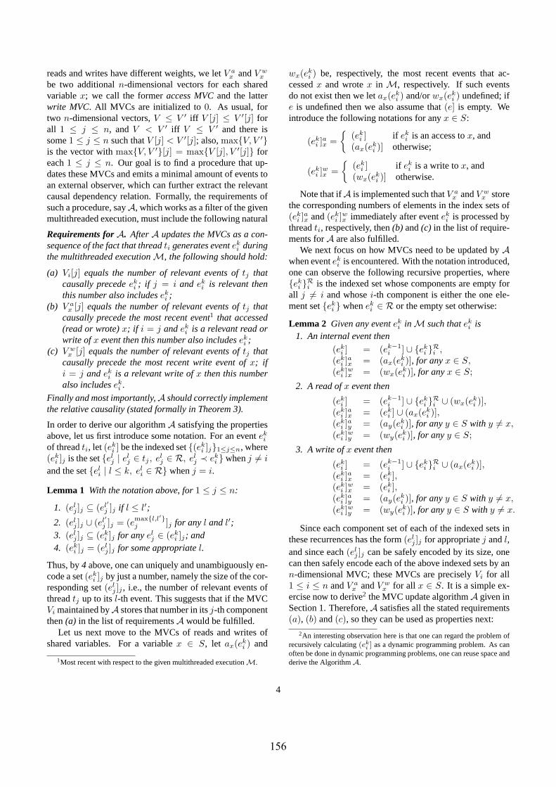
reads and writes have different weights, we letV ax andV w

x

be two additionaln-dimensional vectors for each sharedvariablex; we call the formeraccess MVCand the latterwrite MVC. All MVCs are initialized to0. As usual, fortwo n-dimensional vectors,V ≤ V ′ iff V [j] ≤ V ′[j] forall 1 ≤ j ≤ n, andV < V ′ iff V ≤ V ′ and there issome1 ≤ j ≤ n such thatV [j] < V ′[j]; also,maxV, V ′is the vector withmaxV, V ′[j] = maxV [j], V ′[j] foreach1 ≤ j ≤ n. Our goal is to find a procedure that up-dates these MVCs and emits a minimal amount of events toan external observer, which can further extract the relevantcausal dependency relation. Formally, the requirements ofsuch a procedure, sayA, which works as a filter of the givenmultithreaded execution, must include the following natural

Requirements forA. AfterA updates the MVCs as a con-sequence of the fact that threadti generates eventek

i duringthe multithreaded executionM, the following should hold:

(a) Vi[j] equals the number of relevant events oftj thatcausally precedeek

i ; if j = i and eki is relevant then

this number also includeseki ;

(b) V ax [j] equals the number of relevant events oftj that

causally precede the most recent event1 that accessed(read or wrote)x; if i = j andek

i is a relevant read orwrite ofx event then this number also includesek

i ;(c) V w

x [j] equals the number of relevant events oftj thatcausally precede the most recent write event ofx; ifi = j andek

i is a relevant write ofx then this numberalso includesek

i .

Finally and most importantly,A should correctly implementthe relative causality (stated formally in Theorem 3).

In order to derive our algorithmA satisfying the propertiesabove, let us first introduce some notation. For an eventek

i

of threadti, let (eki ] be the indexed set(ek

i ]j1≤j≤n, where(ek

i ]j is the setelj | el

j ∈ tj , elj ∈ R, el

j ≺ eki whenj 6= i

and the seteli | l ≤ k, el

i ∈ R whenj = i.

Lemma 1 With the notation above, for1 ≤ j ≤ n:

1. (elj ]j ⊆ (el′

j ]j if l ≤ l′;

2. (elj ]j ∪ (el′

j ]j = (emaxl,l′j ]j for anyl andl′;

3. (elj ]j ⊆ (ek

i ]j for anyelj ∈ (ek

i ]j ; and4. (ek

i ]j = (elj ]j for some appropriatel.

Thus, by4 above, one can uniquely and unambiguously en-code a set(ek

i ]j by just a number, namely the size of the cor-responding set(el

j ]j , i.e., the number of relevant events ofthreadtj up to itsl-th event. This suggests that if the MVCVi maintained byA stores that number in itsj-th componentthen(a) in the list of requirementsA would be fulfilled.

Let us next move to the MVCs of reads and writes ofshared variables. For a variablex ∈ S, let ax(ek

i ) and

1Most recent with respect to the given multithreaded executionM.

wx(eki ) be, respectively, the most recent events that ac-

cessedx and wrotex in M, respectively. If such eventsdo not exist then we letax(ek

i ) and/orwx(eki ) undefined; if

e is undefined then we also assume that(e] is empty. Weintroduce the following notations for anyx ∈ S:

(eki ]ax =

(ek

i ] if eki is an access tox, and

(ax(eki )] otherwise;

(eki ]wx =

(ek

i ] if eki is a write tox, and

(wx(eki )] otherwise.

Note that ifA is implemented such thatV ax andV w

x storethe corresponding numbers of elements in the index sets of(ek

i ]ax and(eki ]wx immediately after eventek

i is processed bythreadti, respectively, then(b) and(c) in the list of require-ments forA are also fulfilled.

We next focus on how MVCs need to be updated byAwhen eventek

i is encountered. With the notation introduced,one can observe the following recursive properties, whereek

i Ri is the indexed set whose components are empty forall j 6= i and whosei-th component is either the one ele-ment setek

i wheneki ∈ R or the empty set otherwise:

Lemma 2 Given any eventeki in M such thatek

i is1. An internal event then

(eki ] = (ek−1

i ] ∪ eki Ri ,

(eki ]ax = (ax(ek

i )], for anyx ∈ S,(ek

i ]wx = (wx(eki )], for anyx ∈ S;

2. A read ofx event then

(eki ] = (ek−1

i ] ∪ eki Ri ∪ (wx(ek

i )],(ek

i ]ax = (eki ] ∪ (ax(ek

i )],(ek

i ]ay = (ay(eki )], for anyy ∈ S with y 6= x,

(eki ]wy = (wy(ek

i )], for anyy ∈ S;

3. A write ofx event then

(eki ] = (ek−1

i ] ∪ eki Ri ∪ (ax(ek

i )],(ek

i ]ax = (eki ],

(eki ]wx = (ek

i ],(ek

i ]ay = (ay(eki )], for anyy ∈ S with y 6= x,

(eki ]wy = (wy(ek

i )], for anyy ∈ S with y 6= x.

Since each component set of each of the indexed sets inthese recurrences has the form(el

j ]j for appropriatej andl,and since each(el

j ]j can be safely encoded by its size, onecan then safely encode each of the above indexed sets by ann-dimensional MVC; these MVCs are preciselyVi for all1 ≤ i ≤ n andV a

x andV wx for all x ∈ S. It is a simple ex-

ercise now to derive2 the MVC update algorithmA given inSection 1. Therefore,A satisfies all the stated requirements(a), (b) and(c), so they can be used as properties next:

2An interesting observation here is that one can regard the problem ofrecursively calculating(ek

i ] as a dynamic programming problem. As canoften be done in dynamic programming problems, one can reuse space andderive the AlgorithmA.

4

156

Theorem 3 If 〈e, i, V 〉 and 〈e′, j, V ′〉 are two messagessent byA, thene / e′ if and only if V [i] ≤ V ′[i] if andonly if V < V ′.Proof: First, note thate ande′ are both relevant. The casei = j is trivial. Supposei 6= j. Since, by requirement(a)for A, V [i] is the number of relevant events thatti gener-ated before and includinge and sinceV ′[i] is the numberof relevant events ofti that causally precedee′, it is clearthatV [i] ≤ V ′[i] iff e ≺ e′. For the second part, ife / e′

thenV ≤ V ′ follows again by requirement(a), because anyevent that causally precedese also precedese′. Since thereare some indicesi and j such thate was generated bytiande′ by tj , and sincee′ 6≺ e, by the first part of the the-orem it follows thatV ′[j] > V [j]; therefore,V < V ′. Forthe other implication, ifV < V ′ thenV [i] ≤ V ′[i], so theresult follows by the first part of the theorem.¤

3.1. Synchronization and Shared VariablesThread communication in multithreaded systems was

considered so far to be accomplished by writing/readingshared variables, which were assumed to be knowna pri-ori. In the context of a language like Java, this assumptionworks only if the shared variables are declaredstatic; it isless intuitive when synchronization and dynamically sharedvariables are considered as well. Here we show that, underproper instrumentation, the basic algorithm presented in theprevious subsection also works in the context of synchro-nization statements and dynamically shared variables.

Since in Java synchronized blocks cannot be interleaved,so corresponding events cannot be permuted, locks are con-sidered as shared variables and a write event is generatedwhenever a lock is acquired or released. This way, a causaldependency is generated between any exit and any entry ofa synchronized block, namely the expected happens-beforerelation. Java synchronization statements are handled ex-actly the same way, that is, the shared variable associated tothe synchronization object is written at the entrance and atthe exit of the synchronized region. Condition synchroniza-tions (wait/notify) can be handled similarly, by generatinga write of a dummy shared variable by both the notifyingthread before notification and by the notified thread afternotification.

To handle variables that are dynamically shared, foreach variablex of primitive type in each class the instru-mentation program addsaccessandwrite MVCs, namely_access_mvc_x and_write_mvc_x , as new fields inthe class. Moreover, for each read and write access of avariable of primitive type in any class, it adds codes to up-date the MVCs according to the multithreaded vector clockalgorithm.

3.2. A Distributed Systems InterpretationIt is known that the various mechanisms for process in-

teraction are essentially equivalent. This leads to the follow-

ing natural question: could it be possible to derive the MVCalgorithm in this section from vector clock based algorithmsimplementing causality in distributed systems, such as theones in [3, 7]. The answer to this question is:almost.

Since writes and accesses of shared variables have differ-ent impacts on the causal dependency relation, the most nat-ural thing to do is to associate two processes to each sharedvariablex, one for accesses, sayxa and one for writes, sayxw. As shown in Fig. 3 right, a write ofx by threadi can beseen as sending a “request” message to writex to the “ac-cess process”xa, which further sends a “request” messageto the “write process”xw, which performs the action andthen sends an acknowledgment messages back toi. This isconsistent with step 3 of the algorithm in Fig. 2; to see this,note thatV w

x ≤ V ax at any time.

However, a read ofx is less obvious and does not seemto be interpretable by message passing updating the MVCsthe standard way. The problem here is that the MVC ofxa

needs to be updated with the MVC of the accessing threadi, the MVC of the accessing threadi needs to be updatedwith the current MVC ofxw in order to implant causal de-pendencies between previous writes ofx and the currentaccess, but the point here is that the MVC ofxw doesnothave to be updated by reads ofx; this is what allows readsto be permutable by the observer. In terms of message pass-ing, like Fig. 3 shows, this says that the access processxa

sends ahiddenrequest message toxw (after receiving theread request fromi), whose only role is to “ask”xw send anacknowledgment message toi. By hidden message, markedwith dotted line in Fig. 3, we mean a message which isnot considered by the standard MVC update algorithm. Therole of the acknowledgment message is to ensure thati up-dates its MVC with the one of the write access processxw.

a w a wi x x i x x

Figure 3. A distributed systems interpre-tation of reads (left) and writes (right).

4. The Vector Clock Algorithm at WorkIn this section we propose predictive runtime analysis

frameworks in which the presented MVC algorithm canbe used, and describe by examples how we use it inJAVA

MULTI PATHEXPLORER (JMPAX) [23, 24, 16].The observer therefore receives messages of the form

〈e, i, V 〉 in any order, and, thanks to Theorem 3, can ex-

5

157

tract the causal partial order/ on relevant events, which isits abstraction of the running program. Any permutationof the relevant events which is consistent with/ is calleda multithreaded run, or simply arun. Notice that each runcorresponds to some possible execution of the program un-der different execution speeds or scheduling of threads, andthat the observed sequence of events is just one such run.Since each relevant event contains global state update infor-mation, each run generates a sequence of global states. Ifone puts all these sequences together then one gets a lattice,called computation lattice. The reader is assumed famil-iar with techniques on how to extract a computation latticefrom a causal order given by means of vector clocks [21].Given a global property to analyze, the task of the observernow is to verify it against every path in the automatically ex-tracted computation lattice.JPAX andJAVA -MAC are ableto analyze only one path in the lattice. The power of ourtechnique consists of its ability to predict potential errors inother possible multithreaded runs.

Once a computation lattice containing all possible runs isextracted, one can start using standard techniques on debug-ging distributed systems, considering both state predicates[25, 7, 5] and more complex, such as temporal, properties[2, 5, 1, 4]. Also, the presented algorithm can be used asa front-end to partial order trace analyzers such as POTA[22]. Also, since the computation lattice acts like an abstractmodel of the running program, one can potentially run one’sfavorite model checker against any property of interest. Wethink, however, that one can do better than that if one takesadvantage of the specific runtime setting of the proposedapproach. The problem is that the computation lattice cangrow quite large, in which case storing it might become asignificant matter. Since events are received incrementallyfrom the instrumented program, one can buffer them at theobserver’s side and then build the lattice on a level-by-levelbasis in a top-down manner, as the events become available.The observer’s analysis process can also be performed in-crementally, so that parts of the lattice which become non-relevant for the property to check can be garbage-collectedwhile the analysis process continues.

If the property to be checked can be translated intoa finite state machine (FSM) or if one can synthesizeonline monitors for it, like we did for safety properties[24, 14, 15, 23], then one can analyze all the multithreadedrunsin parallel, as the computation lattice is built. The ideais to store the state of the FSM or of the synthesized monitortogether with each global state in the computation lattice.This way, in any global state, all the information neededabout the past can be stored via a set of states in the FSMor the monitor associated to the property to check, which istypically quite small in comparison to the computation lat-tice. Thus only one cut in the computation lattice is neededat any time, in particular one level, which significantly re-

duces the space required by the proposed predictive analysisalgorithm.

Liveness properties apparently do not fit our runtime ver-ification setting. However, stimulated by recent encourag-ing results in [19], we believe that it is also worth exploringtechniques that canpredict violations of liveness properties.The idea here is to search for paths of the formuv in thecomputation lattice with the property that the shared vari-able global state of the multithreaded program reached byu is the same as the one reached byuv, and then to checkwhetheruvω satisfies the liveness property. The intuitionhere is that the system can potentially run into the infinitesequence of statesuvω (u followed by infinity many repe-titions of v), which may violate the liveness property. It isshown in [19] that the testuvω |= ϕ can be done in poly-nomial time and space in the sizes ofu, v andϕ, typicallylinear inuv, for almost any temporal logic.

4.1. Java MultiPathExplorer (JMPaX)JMPAX [23, 24] is a runtime verification tool which

checks a user defined specification against a running pro-gram. The specifications supported byJMPAX allow anytemporal logic formula, using an interval-based notationbuilt on state predicates, so our properties can refer to theentire history of states. Fig. 4 shows the architecture ofJM-PAX. An instrumentation module parses the user specifica-

Specification

Java

Multithreaded

Program

Bytecode

Compile

Instrumentor

Instrumented

Bytecode

Translator

SpecificationImpl

LTL Monitor

Execute

Level 0

Level 5

Level 4

Level 3

Level 2

Level 1

Computation Lattice

Monitor

Execution Program Execution

JVM

Instrument

Event Stream

Instrumentation

Module Monitoring

Module

Figure 4. The Architecture of JMPAX.

tion, extracts the set of shared variables it refers to, i.e., therelevant variables, and theninstrumentsthe multithreadedprogram (which is assumed in bytecode form) as follows.Whenever a shared variable is accessed the MVC algorithmA in Section 3 is inserted; if the shared variable is relevant

6

158

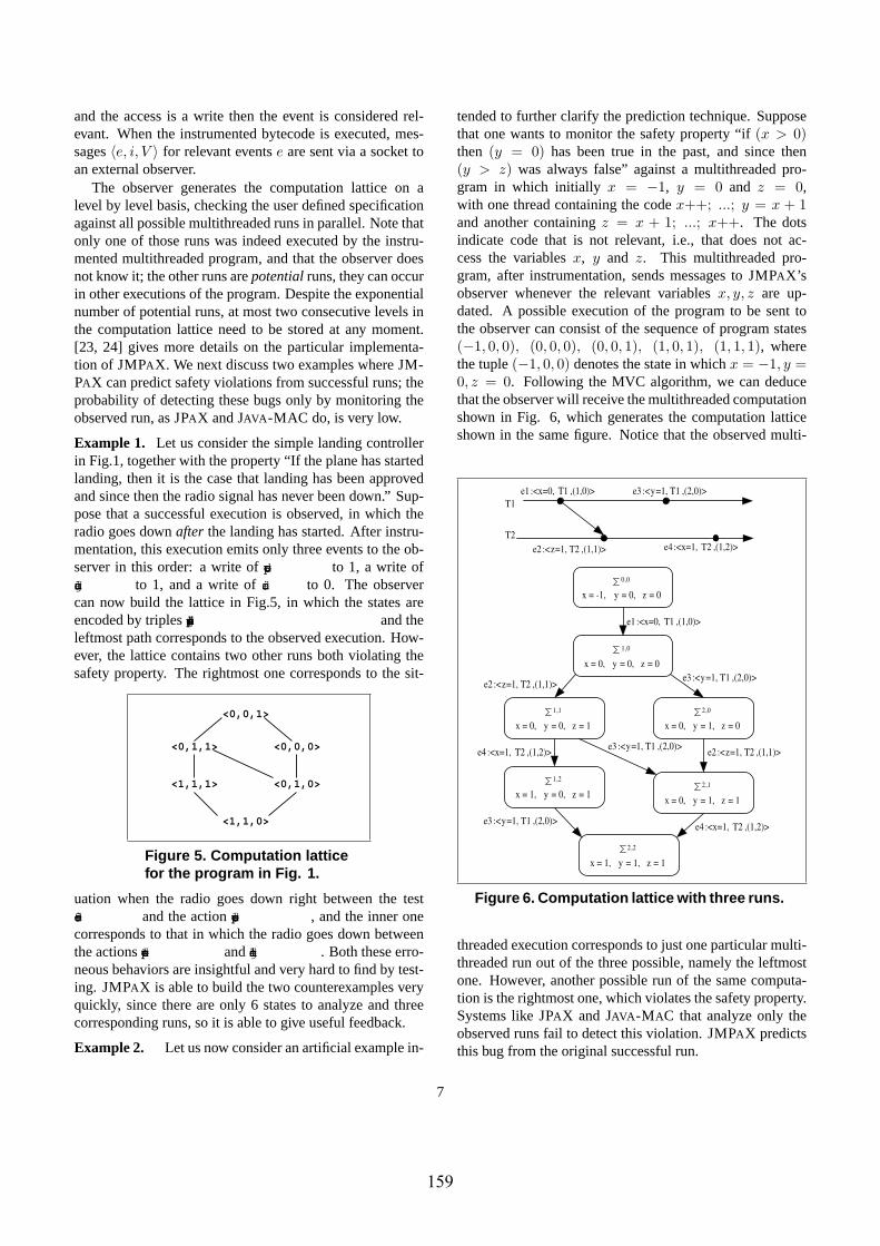
and the access is a write then the event is considered rel-evant. When the instrumented bytecode is executed, mes-sages〈e, i, V 〉 for relevant eventse are sent via a socket toan external observer.

The observer generates the computation lattice on alevel by level basis, checking the user defined specificationagainst all possible multithreaded runs in parallel. Note thatonly one of those runs was indeed executed by the instru-mented multithreaded program, and that the observer doesnot know it; the other runs arepotentialruns, they can occurin other executions of the program. Despite the exponentialnumber of potential runs, at most two consecutive levels inthe computation lattice need to be stored at any moment.[23, 24] gives more details on the particular implementa-tion of JMPAX. We next discuss two examples whereJM-PAX can predict safety violations from successful runs; theprobability of detecting these bugs only by monitoring theobserved run, asJPAX andJAVA -MAC do, is very low.

Example 1. Let us consider the simple landing controllerin Fig.1, together with the property “If the plane has startedlanding, then it is the case that landing has been approvedand since then the radio signal has never been down.” Sup-pose that a successful execution is observed, in which theradio goes downafter the landing has started. After instru-mentation, this execution emits only three events to the ob-server in this order: a write ofapproved to 1, a write oflanding to 1, and a write ofradio to 0. The observercan now build the lattice in Fig.5, in which the states areencoded by triples<landing,approved,radio> and theleftmost path corresponds to the observed execution. How-ever, the lattice contains two other runs both violating thesafety property. The rightmost one corresponds to the sit-

<1,1,1>

<1,1,0>

<0,0,1>

<0,1,1> <0,0,0>

<0,1,0>

Figure 5. Computation latticefor the program in Fig. 1.

uation when the radio goes down right between the testradio==0 and the actionapproved=1 , and the inner onecorresponds to that in which the radio goes down betweenthe actionsapproved=1 andlanding=1 . Both these erro-neous behaviors are insightful and very hard to find by test-ing. JMPAX is able to build the two counterexamples veryquickly, since there are only 6 states to analyze and threecorresponding runs, so it is able to give useful feedback.

Example 2. Let us now consider an artificial example in-

tended to further clarify the prediction technique. Supposethat one wants to monitor the safety property “if(x > 0)then (y = 0) has been true in the past, and since then(y > z) was always false” against a multithreaded pro-gram in which initially x = −1, y = 0 and z = 0,with one thread containing the codex++; ...; y = x + 1and another containingz = x + 1; ...; x++. The dotsindicate code that is not relevant, i.e., that does not ac-cess the variablesx, y and z. This multithreaded pro-gram, after instrumentation, sends messages toJMPAX’sobserver whenever the relevant variablesx, y, z are up-dated. A possible execution of the program to be sent tothe observer can consist of the sequence of program states(−1, 0, 0), (0, 0, 0), (0, 0, 1), (1, 0, 1), (1, 1, 1), wherethe tuple(−1, 0, 0) denotes the state in whichx = −1, y =0, z = 0. Following the MVC algorithm, we can deducethat the observer will receive the multithreaded computationshown in Fig. 6, which generates the computation latticeshown in the same figure. Notice that the observed multi-

S 0 ,0

x = -1, y = 0, z = 0

S 2 ,2

x = 1, y = 1, z = 1

S 2 ,1

x = 0, y = 1, z = 1

S 2 ,0

x = 0, y = 1, z = 0

S 1 ,1

x = 0, y = 0, z = 1

S 1 ,0

x = 0, y = 0, z = 0

e1 :<x=0, T1 ,(1,0)>

e4 :<x=1, T2 ,(1,2)>

e2 :< z =1, T2 ,(1,1)> e3 :< y =1, T1 ,(2,0)>

e2 :< z =1, T2 ,(1,1)> e3 :< y =1, T1 ,(2,0)>

e1 :<x=0, T1 ,(1,0)>

e2 :< z =1, T2 ,(1,1)>

e3 :< y =1, T1 ,(2,0)>

e4 :<x=1, T2 ,(1,2)>

T1

T2

S 1 ,2

x = 1, y = 0, z = 1

e4 :<x=1, T2 ,(1,2)>

e3 :< y =1, T1 ,(2,0)>

Figure 6. Computation lattice with three runs.

threaded execution corresponds to just one particular multi-threaded run out of the three possible, namely the leftmostone. However, another possible run of the same computa-tion is the rightmost one, which violates the safety property.Systems likeJPAX and JAVA -MAC that analyze only theobserved runs fail to detect this violation.JMPAX predictsthis bug from the original successful run.

7

159

5. Conclusion

A simple and effective algorithm for extracting the relevantcausal dependency relation from a running multithreadedprogram was presented in this paper. This algorithm is sup-ported byJMPAX, a runtime verification tool able to detectand predict safety errors in multithreaded programs.

Acknowledgments. Many thanks to Gul Agha and Mark-Oliver Stehr for their inspiring suggestions and commentson several previous drafts of this work. The work is sup-ported in part by the Defense Advanced Research ProjectsAgency (the DARPA IPTO TASK Program, contract num-ber F30602-00-2-0586, the DARPA IXO NEST Pro-gram, contract number F33615-01-C-1907), the ONR GrantN00014-02-1-0715, the Motorola Grant MOTOROLA RPS#23 ANT, and the joint NSF/NASA grant CCR-0234524.

References

[1] M. Ahamad, M. Raynal, and G. Thia-Kime. An adaptiveprotocol for implementing causally consistent distributedservices. InProceedings of International Conference onDistributed Computing (ICDCS’98), pages 86–93, 1998.

[2] O. Babaoglu and M. Raynal. Specification and verificationof dynamic properties in distributed computations.Journalof Parallel and Distr. Computing, 28(2):173–185, 1995.

[3] O. Babaoglu and K. Marzullo. Consistent global statesof distributed systems: Fundamental concepts and mecha-nisms. In S. Mullender, editor,Distributed Systems, pages55–96. Addison-Wesley, 1993.

[4] H. Barringer, A. Goldberg, K. Havelund, and K. Sen. Rule-Based Runtime Verification. InProceedings Verification,Model Checking and Abstract Interpretation (VMCAI 04)(To appear in LNCS), January 2004.

[5] C. M. Chase and V. K. Garg. Detection of global predicates:Techniques and their limitations.Distributed Computing,11(4):191–201, 1998.

[6] E. M. Clarke and J. M. Wing. Formal methods: state ofthe art and future directions.ACM Computing Surveys,28(4):626–643, Dec. 1996.

[7] R. Cooper and K. Marzullo. Consistent detection of globalpredicates.ACM SIGPLAN Notices, 26(12):167–174, 1991.Proceedings of the ACM/ONR Workshop on Parallel andDistributed Debugging.

[8] J. Dick and A. Faivre. Automating the generation and se-quencing of test cases from model-based specifications. InProceedings of Formal Methods Europe (FME’93): Indus-trial Strength Formal Methods, volume 670 ofLNCS, pages268–284, 1993.

[9] C. J. Fidge. Partial orders for parallel debugging. InPro-ceedings of the 1988 ACM SIGPLAN/SIGOPS workshop onParallel and Distr. Debugging, pages 183–194. ACM, 1988.

[10] E. L. Gunter, R. P. Kurshan, and D. Peled. PET: An inter-active software testing tool. InComputer Aided Verification(CAV’00), volume 1885 ofLNCS, pages 552–556. Springer-Verlag, 2003.

[11] K. Havelund and G. Rosu. Monitoring Java Programs withJava PathExplorer. InProceedings of the 1st Workshop onRuntime Verification (RV’01), volume 55 ofENTCS. Else-vier, 2001.

[12] K. Havelund and G. Rosu. Monitoring Programs usingRewriting. In Proceedings Automated Software Engineer-ing (ASE’01), pages 135–143. IEEE, 2001.

[13] K. Havelund and G. Rosu.Runtime Verification 2001, 2002,volume 55, 70(4) ofENTCS. Elsevier, 2001, 2002. Proceed-ings of aComputer Aided Verification (CAV’01, CAV’02)workshop.

[14] K. Havelund and G. Rosu. Efficient monitoring of safetyproperties.Software Tools and Tech. Transfer, to appear.

[15] K. Havelund and G. Rosu. Synthesizing monitors for safetyproperties. InTools and Algorithms for Construction andAnalysis of Systems (TACAS’02), volume 2280 ofLNCS,pages 342–356. Springer, 2002.

[16] Java MultiPathExplorer.http://fsl.cs.uiuc.edu/jmpax .[17] M. Kim, S. Kannan, I. Lee, and O. Sokolsky. Java-MaC: a

Run-time Assurance Tool for Java. InProceedings of Run-time Verification (RV’01), volume 55 ofENTCS. ElsevierScience, 2001.

[18] D. Lee and M. Yannakakis. Principles and methods of test-ing finite state machines - A survey. InProceedings of theIEEE, volume 84, pages 1090–1126, 1996.

[19] N. Markey and P. Schnoebelen. Model checking a path(preliminary report). In Proceedings of the 14th In-ternational Conference on Concurrency Theory (CON-CUR’2003), LNCS. Springer, 2003.

[20] K. Marzullo and G. Neiger. Detection of global state predi-cates. InProceedings of the 5th International Workshop onDistributed Algorithms (WADG’91), volume 579 ofLNCS,pages 254–272. Springer, 1991.

[21] F. Mattern. Virtual time and global states of distributed sys-tems. InParallel and Distributed Algorithms: proceedingsof the International Workshop on Parallel and DistributedAlgorithms, pages 215–226. Elsevier, 1989.

[22] A. Sen and V. K. .Garg. Partial order trace analyzer (pota)for distrubted programs. InProceedings of Workshop onRuntime Verification (RV’03), ENTCS, 2003.

[23] K. Sen, G. Rosu, and G. Agha. Runtime safety analysis ofmultithreaded programs. InEuropean Software EngineeringConference and ACM SIGSOFT Symposium on the Founda-tions of Software Engineering (ESEC/FSE’03). ACM, 2003.

[24] K. Sen, G. Rosu, and G. Agha. Online efficient predictivesafety analysis of multithreaded programs. In10th Inter-national Conference on Tools and Algorithms for the Con-struction and Analysis of Systems (TACAS’04) (To Appearin LNCS), Bercelona, Spain, 2004. Springer.

[25] S. D. Stoller. Detecting global predicates in distributedsystems with clocks. InProceedings of the 11th Inter-national Workshop on Distributed Algorithms (WDAG’97),pages 185–199, 1997.

[26] S. A. Vilkomir and J. P. Bowen. Formalization of soft-ware testing criteria using the Z notation. InProceedingsof COMPSAC 01: 25th IEEE Annual International Com-puter Software and Applications Conference, pages 351–356. IEEE Computer Society, Oct. 2001.

8

160

! "$# %&'() *+-,! .#-%/(0 12(

354768:9<;>=@?ACBEDGFH<9IKJ@LMINPO79IQBED)R6<S<FUT79I)D0R5NP;VTW4XNA5Y4*8 Z6[\AQ]IN^V_`ACBa^4abc!4a_d]<6W^eAQN/?fg;eACBWfCA

h\BW;>i7AQNj8k;>^eJU4abmlSeSe;nB<4a;o8/IK^hNHIKB*Ipc-9IQ_d]IQ;eTaB qsrutmvpwWx-y/zm|syvpwEy~|sy!w~zMrE ur\Ks-Ct

Ug<gm/CPQ/KpjPg 0gjkPC ¡VC¢¡ £PP!¤/¥KC ¥C¦§G¢ §C¥g¨

©K¤ª ©C ¤/¥KC ¥Ce!@G« ¡¦K¬K :p­*>¥§GVK¤® °¯Kjj¬K ¡¥` ¥P©Qj±k¥C²¦¥C¢«C ¡¥Q¥n$Vjj ³p­*>¥­<o ´:µm¶C©Q·¤/¥KC ¥C¦§«mKP!¥Kk¥CV¤M¬Q¢«Cm¸ ¡P·«5¹º»°¼-½¾¿0²:G¦Kg )¥n­aK ¡¦¤s¢¡¦gPGÀ ¡P¤­<¥geG¢X¢¥§Gs ©Kg )¸uCÀgPµ)¹º»o¼-½¾Á¦¬Q ´¨Qg¢7k¥C°¯­*eP¦§ :¤­W¥CeC¢­*>¥­*j ¡P¥nsG« ¡¦K¬K :ÂV³P¨ :¤µXí<jj u:C¢¡¢ ³P¿a ©QWj¥gV¤M¬Q¢«Cs¥n¹Kº»o¼s½¾ÄCen¢«C ¡²j ¥­WCo ´j¬K¢¦C7­*>¥QjPmQKpCe-«C ­*ej :p¥²ju­*>¥°Å:kj ¡¥¥n- ©gM ´eCkM¥nM§G¢¥KKC¢0 g ¡P/ ©g Wen­eP:g ¸À©g a ©C ­Æ¥C¨kP*«WQ¸Ce*¥ekµÇk¥CV¤M¬K¢¦/n¢«C ¡²jE ¥¥gC­*>¥QjP7¤³nj ¥-¥Q ©QQ­Æ¥gk::Q®Q¢¥Q:C¢K g ¡Pu ©g>¥g¬§g©eP¤/¥Q ¡°¯­n:P¦¥KKKKeP¤/¥Q ¡Ck¥CV¤M¬Q¢«CPµÈos¥C>gj ¥:¥gekk ´¢ ³MP²kC¢¡¬C eP¤/¥Q ¡°¯­*e:¥Qo¿¸uÀ«C ¡>¥G¬j ©Qg¥Q ´¦¥K¥e5ÉÊË7ÌÂÍGÎGÏÐ<ÎGÑ-Î0Ò7»ºGË<Ó-KQW­Æ¥K²¦gKG¢ §C¥g ©¤d¸À©C:©±kn­WW­*>¥QjPWQ¸Ce¥nE¥Q ©Q­*>¥Qk:PQ®¢¦¥gPC¢j ¦C :* ©Kg :Kejjk ©QE²:G¢¦C ³¥e/¤/¥G ¥gePM¹º»°¼-½¾mj¥g°¤M¬K¢¦Qµ:ÔE¥Q © ©Qu¢¥§0EQK ©QÀ¤/¥C¡¨ ¥C¦§MG¢ §C¥g ©¤Gn¡¢¢¡¬ ¡eC :s ©g>¥g¬§g©sC¬¤/Qj<¥n°¯Q¤M¨­*¢Pµ)Õa¦KG¢¢ ³¿7¸uCPjQM¥g¬Q«¤­¢:¤Pg g ´¥¥e ©g/G¢ §C¥g¨ ©K¤Ö«ss ¥K¥C¢K:C¢¡¢:M¼-×ÆØ-ÊWÙ<µ

ÚXÛÝÜÞßWàáÀgânßWÞã)äånæ¡çèé°êêPéeé°äéoëå>é°äìíè\îKïKì-ðCêPé!äåñKò¡åÆåeêPé°ê:îQæuóQé°äðgô¡ê:ìÂë

ëVïQõköèëòîgõjäéeé°êkõ:æäé/ò¡îQõäì-óCôêkæ¡ê5ëeógêjõ:òø÷Gõjè:æòøäîGëùWõjäñKòîgú$ê:é »é°äéoëùèPîgñ-ånèPïgôæÆëèPîgñsåeèPò´ôïKéVêë*òî-æ¡öQêögèPéVñQçèé°êùäógêPéoèPæ¡ò¡îQúëVûCë »æ¡êkìüäéGîgê:æ´çäéeýXþÿ@äñQêkôõ:ögêkõkýKò¡îQúòøëaè:îmò¡ì-óCäéeæøèPîQæjæ´êkõköKîCäô´äúûçöKò´õ:öòÆëW÷CîQñKòîgúòîgõPé°êjèëVò¡îQúïCëoêuèjë<èEì!êjè:îCëWäKåCéVêjñïgõ:ò¡îQú/ëoäKå>æ »çèPéVê$êPéeé°äéoëPþîQåVäéVæïQîgèPæ´êkôûù<ñKêëeógòæ´ê·ò¡ì-óKé°êëë°òê5é°êkõjê:îQæmè:ñ »èPîQõjêëù7æ¡öQê$ëVòkêäKåMëVûGëVæ´ê:ìÂësåVäéçöQò¡õköUìäKñKêjôõ:öQêjõ:ýQòîgú$òÆëånêèjëVòðgô¡êé°ê:ìè:òîGëméoèPæ¡öQê:éôòìò¡æ´êkñ0þ ½ öKòÆë/çêèPýQîQêëëòÆë/óCèéVæ¡ò¡õkï »ô¡èPéVôûpõ:éeò¡æ¡ò¡õè:ô7òî5æ¡öQêsõjäîKæ´êKæ<äåEñKòøë°æéVòðïQæ¡êjñpë°ûCëVæ´ê:ìÂëGõjäîQõ:ïKé »éVêkîQõPû5èPîQñ5èjë°ûKîgõ:öéoäîKûéVêëVïgôæÆëuòî5ò¡îKöQê:éVêkîKæ7îgäî » ñKê:æ´êPéVìò¡îKòÆëVìæöCèPæ<ëVò´úîKòø÷GõèPîKæ´ôûò¡îQõPé°êjèë°êëEæ¡öQêMîKïKì-ðCêPéäKåÀëVæøèPæ´êëÀæ´ä!ðgêsèPîgè »ôûkêkñ)þ Ø ëèsé°êëVïgôæ>ù)ìäQë°æëVûGëVæ´ê:ì ðïKò´ô¡ñKêPéëmìïGëVæ*õäîKæ¡ò¡îKïQê-æøäïCë°êuæ¡êëVæ¡òîgú/æøäò´ñKêkîKæ¡ò¡ånûðïQúCëaò¡îMæ¡öQêkòéaò¡ì-ógô¡ê:ì!ê:îQæ´è:æòøäîGëþ½ öQêPé°êÀèé°êEæ´çäóQé°äðgô¡ê:ìÂëXçò¡æösëäånæ¡çèPéVêæ´êëVæ¡ò¡îQú0þ0òéëVæ>ùkæ¡êëVæ »òîgúòøë*úKêkîQê:é°èkôôûñQäîQêò¡îsè:î Q©K¥g ìèPîQîQê:ékæögêmëoäKå>æ´çèé°êÀñKê »

êkô´äóCêPéìïCë°æ<ögè:îQñÂæéoèPîGë°ô´èPæ´ê-æögêséVê ïKòé°ê:ì!ê:îQæøëÀò¡îKæøäëeógêjõ:òø÷GõñûKîCèPìò´õ*õköQêkõkýCëXäîæ¡öQêóKéoäúé°è:ìÖëVæøèPæ´êþPãGêkõäîQñGùæ´êë°æKõjäKêPéoè:úKê

òøëäånæ´ê:îéoèPæ¡öQê:éaôòìò¡æ´êkñCùjõäê:éeò¡îQú/äîQôûsëoäì!êuêKêjõ:ïQæòøäîóGèPæ¡öCëþ½ ä5ìòæ¡ò´úQèPæ´êæ¡öQêp÷géoë°æ*óQé°äðgô¡ê:ìpùXëoäKå>æ´çèé°êäånæ¡êkîò¡îQõkôïQñQêëñKû »îgè:ìò¡õõköQêkõkýCëäîèMëVûCë°æ¡êkì«ëuëVæøèPæ´êòîpäé°ñKêPé<æøäsò´ñKê:îQæò´ånû-óKéoäð »ôêkìÂëèPæ)éeïQî » æò¡ì!êþÀêkõjê:îQæ¡ôûùæögêPé°êögèëðgêjê:îÂëoäì!êòîQæ¡ê:éVêëVæXòîéeïQî » æò¡ì!êEìäîQòæøäéVò¡îQúæ´êkõ:öQîKò ïgêë7çöKò´õ:öóKéoäò´ñKêÀèuôò¡æ¡æ¡ô¡êuìäéVêéeò´úQäé/òîdæ¡êëVæ¡òîgú0þnî æ¡öKòÆëèPóKóKéoäKèkõ:ö0ù7ìäîQòæøäéësèé°êèPïQæ´äìèPæ¡ò »õjèkôôûëVûKîQæögêë°òjêkñ-åÆéoäì èåeäéeìèkô)ëeóCêkõ:òø÷GõèPæ¡ò´äî)þ ½ öQêë°êmìäîQò »æ´äéoëaìèPû/æ¡öQêkîðgêÀñQêPóCô¡äûgêkñ/äKåÆå » ôòîgêåeäéXñKê:ðïQúKúKòîgúäéaäî » ôò¡îQêåeäéñûQîgè:ìò¡õè:ô¡ôû-õ:ögêkõ:ýQòîgúsæöCèPæaëè:åeê:æ¡û-óKéoäóCêPéVæò´êëEèPéVêîCäæGðCê »òîgúKò´äKô¡è:æ¡êjñ/ñïKéeò¡îQúë°ûCëVæ´ê:ì êKêkõkïKæ¡ò´äî)þnîÁæ¡öKòÆëÂóGèógê:éVùçê`èéeúKïQêæ¡ögè:æñòÆëVæéeòðïKæ´êkñÄë°ûCë°æ¡êkìÂë5ìèPû

ðgêêkå>ånêjõ:æ¡òêkôûsìäîKò¡æøäé°êkñ-èPæGéVïKîQæò¡ì!êmèkúQè:òîGëVæ0åVäéVìè:ô¡ôû!ëeóCêkõ:ò »÷Gêkñ-ëoèkånêkæûéVê ïKòé°ê:ì!ê:îQæøëPþû-êkå>ånêjõ:æ¡òêEìäîQòæøäéVò¡îQúCù:çêì!êjèPîîgäæEäîQôû$ôò¡îQêèéêkå>÷0õ:ò´ê:îQõ:ûù0ðïKæè:ôøëoä\ñKêjõkêkîKæé°èkôòkêjñ·ìäîQòæøäé »òîgúMçögêPé°êuåeêPçÖäéaîCäMèkñKñKòæ¡ò´äîgèkôì!êëëoèkúKêë*îgêkêkñæ´äðCêÀóGèjëëoêkñåeäéìäîKò¡æ´äéeò¡îQúpógïéeóCäQëoêëPþ\êpòîQæéoäñKïQõkê!è:î\ê:óQòÆëVæ´ê:ìò´õ!æ´ê:ì »óCäé°èkô0ô¡äKúò´õåeäéñòÆëVæéVòðïQæ¡êjñMýQîgäçô¡êkñQúKêþ\êò´ô¡ôïGëVæé°è:æ¡êæ¡öQêê »óKé°êëëVòêkîQêëëÂäåsæöQòøëpô´äúKò¡õ$ðQû ì!êjè:îCëpäå!ëäì!ê@ëVò¡ì-ógô¡êê »èPì-óCôêëþUê·æögê:î@ëVöCäç ögäç êkå>÷0õ:ò´ê:îKæñKòøë°æéVòðïQæ¡êjñ$ìäîKò¡æ´äéoëìèPûdðgêUë°ûKîQæögêëVòkêjñ@å>é°äì.æ¡öQê ëeóCêkõkò´÷Gêjñ é°ê KïKòéVêkì!ê:îKæÆëþ0ò »îgèkôôûùgçê-ñQêë°õ:éeòðgêsèsñòÆëVæéeòðïKæ´êkñ5ëVûCë°æ¡êkìÂëmèóKóCôò´õjè:æòøäîÂñKêêjô »äógì!ê:îKæaå>é°è:ì!êPçäéeý0ùKõjè:ô¡ô¡êkñ ¼-×ÆØ-ÊWÙ þ ½ äïCëoê ¼-×ÆØ-ÊWÙ ù0èïCëoêPéìïCë°æKóQé°äKò¡ñQêÀèPîèóQógôò¡õèPæ¡ò´äîæ´äKúKê:æ¡öQê:é7çò¡æösæ¡öQêuåVäéVìè:ôCëoèkånêkæûóKéoäóCêPéVæò´êë<æöCèPæXë°öQêçèPîQæøëìäîKò¡æ´äéVêjñ0þ ¼s×>ØsÊWÙ è:ïKæøäìèPæ¡ò´õjè:ô¡ôûëVûQîKæ¡öQêë°òjêëõjäKñKêåVäéWìäîQòæøäéVòîgú/æ¡öQêëVógêkõkò´÷0êkñMéVê ïQòé°ê:ì!êkîKæÆëèPîgñ/çêjèêëWèóQóKéoäóQéeòøèPæ´êòîGëVæéeïQì!ê:îKæøèPæ¡òøäîõjäKñKêò¡îKæøäæ¡öQêÀúKòê:îèóQógôò¡õèPæ¡ò´äî)þ ½ ögêèé°õ:öKò¡æ´êkõ:æ¡ïé°êEäå ¼-×ÆØ-ÊWÙ òøëXò´ô¡ôïGëVæé°è:æ¡êjñò¡î0ò´ú »ïé°ê þ½ öQê/çäéeýóQéVêë°êkîKæ´êkñ-ò¡îæ¡öKòÆëóCèPógê:éçèjëuë°æò¡ìïQô´èPæ´êkñðQû!æ¡öQêäð0ë°êPé!èPæ¡òøäî/æ¡ögè:æGòî-ìèPîKûMñòÆëVæéVòðïQæ¡êjñ-ë°ûCëVæ´ê:ìÂëùKë°ïQõkö-èë*çòé°ê »ôêëëëoê:îCëäéîQêkæ¡çäéeýGëùgò¡æ<òÆë" ïKò¡æ´êMò¡ì-óKéoè:õkæò´õjèkô7æ´äÂìäîQòæøäéé°ê »

ïQòé°ê:ì!êkîKæÆëÀêKóKé°êëë°êkñòîõjô¡èëë°ò¡õè:ôWæ´ê:ì-óGäéoè:ôaô¡äKúò´õëPþ#)äéuê »èPì-óCôêùPõäîCë°ò¡ñQêPé)èÀëVûGëVæ´ê:ì äåCìäðQò´ôêîgäKñKêë0ò¡î/çöKò´õ:ö/äîQêìä »ðQò´ôê/îgäñQêmìèPû-é°ê ïgêë°æ7èõjêPéVæ´è:òî$èkôïgêåÆéoäì"èPîCäæ¡öQêPé<ìäðQò´ôêîgäKñKêþ&%mîÂéVêjõkêkòò¡îQú-æ¡öQê/éVê ïQêëVæ>ùKæögêsëoêkõjäîQñîCäñQê/õjäì-óQïKæ´êëæögêèkôïgêèPîgñ-éVêkæïKéeîGëEò¡ænþ Ø îò¡ì-óCäéVæøèPîKæ0éVê ïKòé°ê:ì!ê:îQæ0ò¡î5ëVïgõ:öèpë°ûCë°æ¡êkì'òøëæ¡ögè:æîCä·îCäñKê!éVêjõkêkòêëèé°êPóCôûUåÆéoäì èîgäKñKêæ´äçöKò´õ:öò¡æögèjëîgäæ<óKé°êòøäïGë°ôû·òøëëVïgêkñ$èéVê ïQêëVæeþ'næòÆëêjèëVû\æ´äë°êjêuæ¡ögè:æ ¾ òîgêjèé ½ ê:ì-óGäéoè:ô ¾ äúKò¡õ( ¾g½<¾*) çäïQô¡ñ/îCäæQðgêèóQé°èkõ »æò´õjèkôgëVógêkõkò´÷0õjèPæ¡òøäî/ô´èPîQúKïgèkúKêEåeäé7èPîKûéVêèjëoäîgèPðgôû/ë°òjêkñ/õäô¡ôêjõ »

161

Specification Distributed Program in

Java

Bytecode

Compile

Instrument or

Instrumented Bytecode

MonitorImpl

PT - DTL Monitor

Execute

Program Execution

JVM

Instrumentation Module

Monitoring Module

!#"%$&(')

æòøäîäKå0îgäKñKêëþ ½ äïCë°ê ¾Q½<¾ ùjçêÀçäïQô¡ñîQêjêkñæøäõjäKôô¡êkõkæQõäîCë°òøë »æ¡êkîKæ*ëVîCèóGë°ögäæøëuäåæögêMúQô¡äðCèkôaë°ûCëVæ´ê:ì+*0èìäîQòæøäéçäïgôñæögê:îõ:öQêjõ:ýæ¡öQê-ëVîgèPóGë°ögäæÆëEåVäéóCäQëëVòðgô¡êKò´äKô¡è:æòøäîGëäå*æögêóKéoäóCêPéVæûðQûÂõäîGëVò´ñKêPéVò¡îQúèkôôXóCägëë°òðCôêMòîQæ¡ê:éVô¡êjèKòîgúgëuäåEêê:îQæøëæöCèPæ<èé°êè:ô¡ô¡äçêjñðQûmæ¡öQêEñòÆëVæéeòðïKæ´êkñõjäì-óQïKæøèPæ¡òøäî)þ!eîèEë°ûCë°æ¡êkìüäågæ¡ögäï »ëoèPîgñgëäåaîCäñKêëùõjäô¡ô¡êkõ:æ¡ò¡îQúsë°ïQõköèmúQô¡äðCè:ô0ë°îgèó0ëVöCäæGçäïQô¡ñðgêóKéoäöKòðQò¡æ¡òêþÿ@äé°êjäê:éVùæ¡öQêuîKïQì-ðgêPéXäKå0óGäQëëVòðgô¡êòîQæ¡ê:éVô¡êjèKòîgúgëæ´äuðgêEõäîCë°ò¡ñQêPé°êkñçäïQô¡ñðgêEô¡èPéeúQêêêkîò´åCóGäçêPé°å>ïgôkæ´êkõköKîKò ïgêëëVïQõköMèjëWóCèPéeæ¡òøè:ôCäé°ñKêPéXéVêjñïgõ:æ¡ò´äîèé°êuïGë°êkñ)þ½ äèkñKñé°êëë*æögê/èðCä&êñKò¡ån÷Gõ:ïgôæ¡ûùçêñKêj÷GîQê ­aQ ´¨> ´«¤mG«P¨

¡¦K¬K :M :¤­W¥CeC¢g¢¦¥§G ( ¹º»°¼-½¾ ) þMë°òîgú ¹Kº»o¼s½¾ ùäîgêuõèPîõ:öQêjõ:ýèMóKéoäóCêPéVæûëVïgõ:öèjëæögê!äîQêèPðCäêðQû·öCèò¡îQú·è-ô´äõjèkôìäîKò¡æøäéäî!êè:õköîgäñQêþ)äéEêgè:ì-ógô¡êùîgäñQê

aìäîQòæøäéë-,ò´å

aögèjë7éVêjõkê:ò êkñ/è è:ôïQêEæ¡öQê:îòægìïCë°æKðCêæögêuõèjë°êÀæöCèPæQóKé°êòøäïCëoôûòîæ¡öQêEóGèjë°ægèPæ

bæ¡öQêåVäô¡ô¡äçò¡îQúögêkô¡ñ

bögèëaõjäì-óQïQæ¡êjñæ¡öQê è:ôïQê

èPîQñ/è:æaèEé°ê KïQêëVæKçèjëWìè:ñKêuåeäé)æöCèPæè:ôïQêEò¡î/æ¡öQêóGèjë°æ/.Kþ ½ öKòÆëòøëóQéVêjõ:òÆë°êkôû èPîQñõäîQõkòøëoêkôûUêóKé°êëë°êjñðgûUæ¡öQê ¹º»o¼-½¾ åeäé »ìïQô´è&

receivedV alue→@b( 0 · (computedV alue ∧@a( 0 · requestedV alue)))

1 äæ´ê·æöCèPæçê·é°êjèkñ@èjë2,:è:æ/.ù

@bFòÆë-æ¡öQê è:ôïQê$äKå

Fò¡î

æögê-ìäQëVæ<éVêjõkê:îQæ*ô´äõjèkôë°æ´è:æ¡êäKåbæ¡ögèPæ*æögê!õ:ïKéné°ê:îQæaóKéoäõkêëëòÆëèPçèé°ê/äåoùKè:îQñ 0 · ñKê:îCäæ´êëæ¡öQê/åVäéVìïQô´èmçèjëæéeïgêMëoäì!ê:æ¡òì!êò¡îæögêEóCèëVæeþPÿ äîKò¡æ´äéeò¡îQúmæ¡öQêuèPðCäKêåeäéeìïgô¡èò¡î äKô KêëWë°êkîQñKòîgúîgä

è:ñKñKòæ¡òøäîgèkô)ì!êëëè:úKêë3·ò¡æWòîäKô êëEò¡îCëoêPéVæò¡îQúpäîQôû·èMåeêPç ðgòæÆëäåGò¡îQåVäéVìèPæ¡ò´äîçöKò´õ:öMèPéVêEógò¡úQúûKðCè:õkýKêkñäîæ¡öQêÀì!êëëè:úQêëaæ¡ögè:æèé°êEèkô¦é°êjèkñûðgêkòîgúuóGèjëë°êkñmò¡îæögêõjäì-ógïKæøèPæ¡ò´äî)þ ½ öKòÆë)êjå>÷Gõkò¡êkîQõPûóKéoäò´ñKêë)èÀë°ïðGë°æ´è:îKæ¡ò´èkôò¡ì-óKéoäê:ì!êkîKæäê:éGçöCèPæòÆëXé°ê KïKòéVêjñæøäìäîKò¡æøäéXåVäéVìïQô´èjëaçméVò¡ææ´ê:îMòîsõkô´èjëë°ò¡õè:ô ¾g½<¾ þ

\ê5òîQæéoäñKïQõjê eP¤/¥g p°¯­n:P¦¥KK òî ¹º»o¼-½¾ æ´äéVê:óKé°ê »ë°êkîKæ*èkôïgêëmçöKò´õ:ö$èPéVêånïKîgõ:æ¡ò´äîCëñKê:ógêkîQñò¡îQú5äî·æ¡öQêë°æ´è:æ¡êÂäåèmé°ê:ìäæ´êóQé°äKõkêëëþ )äéEêgè:ì-ógô¡êùQèóQé°äKõkêëëìèPûìäîKò¡æøäé*æ¡öQêóKéoäóCêPéVæû 4,ò´å)ìû-è:ô´èéVì ögèë7ðgêjê:îë°ê:æCæ¡öQêkî/òæCìïGëVæQðgêÀæ¡öQêmõjèë°êæöCèPææ¡öQêuñò´åÆånê:éVêkîQõjê<ðCê:æ´çêkê:îìûæ´ê:ì-óCêPéoèPæ¡ïé°êEè:îQñæ¡öQêEæ´ê:ì-óCêPé »èPæ¡ïé°ê/èPæXóKéoäõjêëë

bêQõkêjêkñQêkñ-æ¡öQê/è:ô¡ô´äçêkñ$èkôïgê5.þ ½ öQòøëEòøëÀê »óKé°êëë°êkñMèjë

alarm→ 0 · ((myTemp−@botherTemp) > allowed)

6 êPé°ê@botherTemp

òÆë5è$éVêkìäæ´ê\êKóKé°êëëVòøäî æöCèPæòÆë·ëVïð »æéoè:õkæ¡êjñ/å>é°äì æögêuô´äõjèkô#èkôïgêuäåmyTemp

þØ îêgèPì-óCôêäåGèëoèkånêkæûóKéoäóCêPéVæûæöCèPæìèPûðgêïCëoêkånïQôjòîæ¡öQêõjäîKæ´êKæaäåEèPîpè:òéeógô´èPîgêsëäånæ¡çèé°ê/òÆë7,Pò¡åìûpè:òéeógô´èPîgê/òÆëÀô´èPîgñ »òîgúuæ¡öQêkîæ¡öQêéVïKîgçè:ûmèkôô´äõèPæ´êkñuðQûmæögêè:òéeóCäéeæìèPæ´õ:ögêë0æögêäîQê

æöCèPæ<èPì óCô¡è:îKîQòîgúæ´äïCëoê5.Kþ ½ öQòøëWóKéoäóCêPéVæû/ìè:û/ðCêêKóKé°êëë°êkñòî ¹º»°¼-½¾ èjë*åeäKôô´äçëlanding→ (runway = (@airportallocRunway))

ÿ è:îûMéVêë°êjèPéVõköQê:éoë<ögèêóQé°äóCäQëoêkñæ¡êkì-óCäéoè:ôgô´äúò´õë*æøäéVêè »ëoäîpèðGäïQæXñòÆëVæéVòðïQæ¡êjñÂëVûGëVæ´ê:ìÂëþKÿ ägëVæWäå*æögêë°êsô´äúò´õëÀèé°ê/ò¡î »ëeógòé°êkñðQûæ¡öQêõjô¡èëë°ò¡õÀçäéeýäKå Ø ïKìè:îKî98/:<;XèPîgñ 6 èkô¦óCêPéVî k G¢¦µ8>=?;äîÂýQîgäçô¡êkñQúKê/ò¡î5ñòÆëVæéeòðïKæ´êkñ5ëVûCë°æ¡êkìÂëþgÿ êkê:îCèPýGëVöKò k 7G¢¦µñKê÷CîQêè/ýKîCäçôêjñKúKêæ´ê:ì-óGäéoè:ô0ô´äúKò¡õòîQæ¡ê:énóQéVêkæ¡êjñ!äê:éèì!êë »ëoèkúKêÂëoê ïgê:îgõkêõ:öCèéVæøëòîè!ñòÆëVæéVòðïQæ¡êjñ$ëVûCë°æ¡êkì@8 5AB;è:îQñ·ñQê »êkô´äó·ì!êkæöCäñgëåVäéÀìäKñKêkôWõköQêjõ:ýKò¡îQú5åVäéVìïQô´è:êMòî·æ¡öKòÆëô´äúKò¡õKþ%mïéõäììïQîKò´õjèPæ¡òøäî!óQéeò¡ìò¡æòKêsçèëmòî5óGèéVæ<ò¡îCëeógòé°êkñÂðgû·æöQòøëçäéVýGùPðïKægçêuè:ô¡ô¡äçèPénðgòæé°èPéeûêKóKé°êëëVòøäîCë7è:îQñè:æ´äìò¡õóQé°äóCä »ëVò¡æòøäîGë<äKêPé7êóKé°êëëVòøäîGë7òîMæögê:òéaô´äúKò¡õKþØ îgäæ¡öQê:éõkô´äQëoêkôû éVêjô¡è:æ¡êjñ çäéeýòÆëpæ¡ögèPæsäå(C)êkîQõkê:ýD8!E=gù

4FG;çöQò¡õkö ñKêj÷GîQêësèpæ´ê:ì-óGäéoè:ôô¡äKúò´õ5äKåõjè:ïCëoèkôýKîCäçôêjñKúQêþÉ îgäçô¡êkñQúKêäóCêPéoèPæøäéëXèPéVêóKéoäò´ñKêjñuæøämé°êjèjëäîèPðCäïQææ¡öQêÀô´äõè:ôöKòÆëVæøäéVûÂäåEè/óKéoäõkêëëùCèjëuçêkô¡ôWèjëèðCäïKæXæögêýQîgäçô¡êkñKúQêòæ<èkõ » ïQòé°êëå>é°äì&äæögêPé<óQé°äKõkêëë°êëþ 6 äçêêPéVùòîpäé°ñKêPé<æøä-ýKêjêPó!æ¡öQêõjäì-ógô¡êKò¡æûäKå<ìäKñKêkôXõ:ögêkõ:ýQòîgúæé°èkõ:æøèðgô¡êùHCXê:îQõkêkýñQäKêëîCäæè:ô¡ô¡äç æ¡öQê-îQêëVæ¡òîgú·äåÀõèPïCëè:ôWýQîgäçô¡êkñQúKê-äógê:é°è:æ´äéoëPþ eîKæ´êPé°êë°æ »òîgúKôûùGæögêîQêëVæ¡òîgúäåõjèPïGëoèkô<ýKîCäçôêjñKúQêsäógêPéoèPæøäéëmñQäKêëîCäæè:ñQñèPîûsõjäì-ógô¡êKò¡æûæøääïé<è:ô¡úQäéeò¡æöQìüåVäéaìäîQòæøäéVò¡îQú0þ¾ ê:ïgõ:ýKê:éÂò¡î KêëVæ¡ò´úQèPæ´êëpôò¡îQêjèPéÂæ´ê:ì-óGäéoè:ôô´äúKò¡õ@òîQæ¡ê:énóQéVêkæ¡êjñäê:éué°êëVæéVò¡õkæ¡êjñô¡èPðgêjôêjñ·óCèPéeæ¡òøè:ôEäé°ñKêPéëõè:ô¡ôêjñÿ@èkïéVýKò´êPçò¡õ

æéoè:õjêë%8 JIH;þ Ø îäê:é Kò¡êPç äåEñKòøë°æéVòðïQæ¡êjñÂôò¡îQêjèPéæò¡ì!êæ´ê:ì-óGä »é°èkôWô¡äKúò´õëðCèë°êkñ5äî5ÿ@èkïéVýKò´êPçò¡õ/æé°èkõkêëòÆëmúòKê:î!ðgû ½ öKòøè »úQèPé°è:îLKèPî k *C¢µ ò¡îM8/IHI<;þ Ø ôïé k *C¢µ 8N;Àò¡îKæé°äKñïgõkê!èæ´ê:ì-óGä »é°èkôô¡äKúò´õäKåCõjèPïGëoèkôò¡æû( ½¾PO") çöKò´õ:ömòøëXò¡îKæ´êPéeóKé°ê:æ´êkñmäêPéGõjè:ïCëè:ôëVæéeïgõ:æ¡ïé°êë)õjäéné°êëVóCäîgñò¡îQúæøäÀóGèéVæòøè:ôäéVñQêPéGêKêkõkïKæ¡ò´äîCë)äåGèñòÆë »æéVòðïKæ´êkñëVûGëVæ´ê:ì·þ ½ ögêPûïCëoêðCäæö-óGèjë°æaè:îQñånïKæ¡ïé°êæò¡ì!êäóCêPéoè »æ´äéoë*èPîgñúò êuèuìäñKêjôKõköQêkõkýKò¡îQú/èkôúgäéVòæ¡öKì åVäéaæögêuô´äúò´õþnî·é°êkõjê:îQæ*ûQêèéëù)æ¡öQê:éVêöCèjëðCêkêkî$õjäîCëVò´ñKê:é°èPðgô¡ê-òîQæ¡ê:éVêëVæòî

éeïQîKæ¡òì!ê ê:éeòø÷Gõjè:æòøäîQ8!E;oþ 6 èêjôïQîQñ k mC¢µ 8 JRH;-úòKêèkôúgä »éeò¡æ¡öKìÂëmåVäéë°ûKîKæ¡öQêëVò:ò¡îQú·êjå>÷Gõ:ò´ê:îQæ<ìäîQòæøäéëåeäéëoèkånêkæûóKéoäó »êPéVæò´êëPþãGêkî j QC¢µ 8/IHR<;7ñKêêjô¡äóæ´êkõ:öQîKò ïgêëaåVäéaéVïKîKæ¡ò¡ì!êëoèkånêkæûèPîCè:ôûCëVòÆëåVäé<ìïQôæ¡òæ¡öé°êjèkñKêkñóKéoäúé°è:ìÂë*è:îQñ-ò¡îKæé°äKñïgõkêæögêæ´äQäôS ÿTC ÙVU þ)ã)äì!ê!äæ¡öQê:ééeïQîKæ¡òì!ê ê:éeòø÷GõèPæ¡ò´äîë°ûCë°æ¡êkìÂëòîgõkôïQñKêS C)è U åÆéoäì 1 Ø ã ØÁØ ì!êëP8>W?;7è:îQñ XCY 1X1 «ë<ÿ@è:õ8 #E;oþ

162

UêõjèPî-æ¡öKò¡îKý!äåWè:æ)ôêèjë°æ0æöKéVêjêuìèKäé*õjäîKæéeòðïKæ¡ò´äîCë*äåaæ¡öQêçäéeý!óKé°êë°êkîKæ´êkñò¡îpæöQòøëóCèPógêPéVþ&0òéëVæ>ùCçêsñKêj÷GîQêè-ëVò¡ì-ógô¡ê/ðïQæêóQéVêëëVò ê-ô¡äKúò´õ-æ´äëVógêkõkò¡ånû\ëoèkånêkæûóKéoäógê:éeæ¡ò´êëuòî\ñòÆëVæéeòðïKæ´êkñëVûCë°æ¡êkìÂëþ:ãGêjõjäîgñCùkçêEóQé°äKò¡ñQêè:îMè:ô¡úQäéeò¡æ¡öKìÄæøä/ëVûQîKæ¡öQêëVòkêñKê »õkê:îQæéoè:ôòkêkñìäîQòæøäéëXåeäéaëoèkånêkæûmóQé°äógêPéVæ¡ò¡êë0æ¡ögè:æQèé°êêKóKé°êëëoêkñòî·æ¡öQê!ô´äúKò¡õKþ0òîCè:ô¡ôûù)çê!ñKêë°õPéVòðgê-æ¡öQêò¡ì-ógô¡ê:ì!êkîKæøèPæ¡ò´äî5äKåuèæ´äQäô ( ¼-×ÆØ-ÊWÙ ) æöCèPæ*òÆëðCèjëoêkñ$äîæ¡öKòÆëmæ¡êjõ:öQîKò ïQêKþ ½ öQêæøäKäKô<òÆëóQïðCôò´õkôûèèPò´ô´èðgô¡êuåVäéWñQäçîgô¡äQè:ñ)þ½ öQêé°êë°æaäKå*æ¡öQê/óCèPógêPéEòÆëuäéeúQè:îKòkêjñ-èëÀåVäô¡ô´äçëþKãGêjõ:æ¡ò´äî IèPîQñ5ãGêjõ:æ¡ò´äîÂúKòêsæögêMóKé°êkôòìò¡îgèPéeò´êëPþQãGêkõkæòøäîN5ò¡îKæé°äKñïQõjêë

¹º»°¼-½¾ þeîãGêkõkæòøäî :çêÀñQêëoõPéVòðCêæ¡öQêÀèkôúgäéVòæ¡öKìÄæöCèPæïQîQñKê:é »ôò´êëäïKéXò¡ì-ógô¡ê:ì!ê:îQæ´è:æòøäîXþ:ãGêkõkæòøäî9AðQéeò´êCûsñKêë°õPéVòðgêëWæögêÀò¡ì »ógô¡ê:ì!ê:îQæ´è:æòøäîèkô¡äîQú/çò¡æ¡öò¡îKò¡æòøè:ôCêKógêPéVò¡ì!ê:îKæøèPæ¡òøäî)þ*ÛUângânáCà WÖØ ñKòøë°æéVòðïKæ´êkñëVûGëVæ´ê:ì òÆë<èõäô¡ôêjõ:æ¡ò´äîMäå

nóKéoäõkêëëoêëWäéaè:õ »æ´äéoë

(p1, . . . , pn)ù7êè:õköçòæ¡öò¡æøëäçîô¡äKõjè:ôEëVæøèPæ´êþ ½ ögê!ô´äõjèkôëVæøèPæ´ê-äKåè/óQé°äKõkêëëÀòøëmúKòê:îðQûpæögê è:ôïQêëðCäïKîgñæ´äÂò¡æøë èPéeò »èðgô¡êëPþ 1 äæ´êEæöCèPææ¡öQê:éVêèé°êEîgäúQô¡äðCèkôäéaë°ögèé°êkñèPéeòøèðCôêëþ CGé°ä »õkêëë°êësõjäììïQîKò´õjè:æ¡êÂçòæ¡ödäæ¡öQê:éïGëVò¡îQú èjë°ûKîgõ:öéoäîCäïGëì!êë »ëoè:úQêëXçögägë°êÀäéVñQêPé)äå0èPénéVòè:ôòÆëXò¡îQñKêkæ¡ê:éeìò¡îgè:æ¡êKþ ½ ögêEõjäì-ógïKæøè »æòøäî/äåGêè:õköóQé°äKõkêëë)òøëaèPðGë°æéoè:õkæ¡ôûìäñKêjôêjñðgûèÀëoê:æQäKå P²j:g ùèPîQñMèuñKòøë°æéVòðïQæ¡êjñ/õjäì-óQïQæ´è:æòøäîòÆëëVógêkõkò´÷0êkñðgûsèóCèéVæ¡ò´èkôgäéVñQêPé

≺äîæ¡öQêêê:îQæøëPþ ½ öQê:éVêèé°êuæ¡öé°êkêæ¡ûóCêë*äå7êê:îQæøëþ «C VQC¢ êKê:îKæÆëWõkögè:îQúKêÀæögêuô´äõjèkôCë°æ´è:æ¡êäåaèÀóKéoäõkêëëJ*I0þ :K êê:îQæøëWõjèPïGë°êmèóQé°äKõkêëëaæøäMëoê:îQñsèÀì!êëëè:úKê?*è:îQñCþ ekk¦² êêkîKæÆëEäõkõkïéçögê:îÂèì!êëëè:úQêòøëEéVêjõkêkòêkñsðgûèóKéoäõjêëëPþ

¾ ê:æEi

ñKêkîgäæ¡êæ¡öQêëoê:æWäå<êêkîKæÆëEäåaóQé°äKõkêëëpi

èPîgñôêkæEñKê »îgäæ´ê ⋃

i Ei

þ 1 äçù⊆ E ×E

òÆë*ñQêj÷Cîgêkñèë<åVäô¡ô´äçëþ

e

e′ò´å

eèPîgñ

e′èPéVêêêkîKæÆë*äKåXæ¡öQê/ëèPì!êóKéoäõjêëëèPîgñ

eögèPóKógêkîCëXò¡ìì!êkñKò´è:æ¡êjôûðCêkåVäé°êe′ù

I0þe

e′ò¡å

eòøë*æ¡öQêë°ê:îgñMêKê:îKæ0äKåaèì!êëëoèkúKêèPæXëäì!êuóKéoä »õkêëë/è:îQñ

e′òøëæögê!õjäéné°êëVóCäîgñò¡îQúéVêjõkêkòêêêkîKæäKåÀæ¡öQê

ì!êëëoè:úQêè:æQæ¡öQêÀéVêjõ:òóQò´ê:îKæQóKéoäõjêëëþ½ öQê/óCèéVæ¡ò´èkô7äéVñQêPé

≺òøëÀæögêæéoèPîCë°òæ¡òêMõkô´äQë°ïé°êMäåæ¡öQêéVêjô¡è:æòøäî

-þ ½ öQòøë)óGèéVæòøè:ôäé°ñKê:é0õjèógæïKéVêëGæ¡öQê :C¬C¢¡ ³ éVêjô¡è:æòøäîmðgêkæ¡çêjê:îêê:îQæøëPþ ½ ögê·ë°æéVïQõkæïKéVêpñKêë°õ:éeòðgêjñðgûC = (E,≺)

òøësõè:ô¡ôêjñè C¦ ´K¬ ¡P$:¥K¤­*¬K ¦C ¡¥ èPîQñ·çê!èëë°ïKì!ê!èPî$èPénðgòæéoèéVûÂðïQæúòêkîMñKòøë°æéVòðïQæ¡êjñMõäì-ógïKæøèPæ¡ò´äî

Cþ0ïKéeæ¡öQê:éVùÁòÆëæ¡öQêéVêGêQòê

èPîQñ/æéoèPîGëVò¡æòKêuõkô´äQë°ïé°êuäå-þeî0ò´ú0þ4ICùe11 ≺ e23

ùe12 ≺ e23

ùèPîQñ

e11

e23þ 6 äçêêPéVù

e12 6

e23þ

)äée ∈ E

ù0çê-ñKê÷CîQê↓e

def= e′ | e′

eùgæ¡ögèPæWòÆëù

↓eòøëæ¡öQêëoê:æ7äKåWêê:îQæøë*æ¡ögè:æ)õjè:ïCëoèkôôû-óKé°êkõjêkñQêeþ )äé

e ∈ Ei

ùKçêõjèPîMæöQòîQý-äKå

↓eèjë<æögêô´äõè:ô)ë°æ´è:æ¡êäå

pi

çögê:îsæögêêKê:îKæeöCèjë

K°ïGëVægäKõkõkïéeéVêjñ0þ ½ öKòÆë*ë°æ´è:æ¡êõjäîQæ´è:òîGë7æ¡öQêöQòøë°æ´äéeûäKå)êêkîKæÆëWäå7è:ô¡ôóKéoäõkêëëoêë7æ¡ögè:æCõèPïGëoè:ô¡ôûóKé°êkõjêkñKêeþ

Uê!êKæ´ê:îgñæ¡öQê-ñQêj÷CîQòæ¡ò´äî5äKåMù≺èPîgñ æøä5ô¡äKõjè:ô*ë°æ´è:æ¡êë

ëVïQõköMæ¡ögè:æ↓e

↓e′

ò¡åÆåe

e′ù↓e ≺ ↓e′

ò´åÆåe ≺ e′

ùKèPîgñ↓e

↓e′

ò¡åÆåe

e′þ\êñKê:îCäæ´êÀæ¡öQêë°êkæ)äåaô¡äKõjèkôGë°æ´è:æ¡êëäåWèóQé°äKõkêëë

m1

p3

p2

p1

e31 e32 e33

e22 e23

e11 e12

m4

m3

m2

! " #" %$&('X)* )+

pi

ðQûLSi

def= ↓e | e ∈ Ei

è:îQñpôêkæLS

def=

⋃

i LSi

þ#\êïCëoêæögêuëVûQì-ðCäôøë

si, s′i, s

′′i , . . .

æøämé°êPóKé°êëoê:îQææögêô¡äKõjèkôgëVæøèPæ´êë<äåóKéoäõjêëë

pi

þ\êpè:ôøëoä·èjëëVïQì!ê-æöCèPæ<æ¡öQêô´äõè:ôë°æ´è:æ¡êsi

äåêjèkõ:öóKéoäõjêëë

pi

èjëëoäKõ:òøèPæ´êë*è:ôïQêë<æøäsëäì!êmô¡äKõjè:ôèéVòøèðgô¡êëVi

ùKèPîQñæöCèPæ

si(v)ñQê:îgäæ¡êë7æ¡öQê èkôïgêÀäåXè èéVò´èPðgô¡ê

v ∈ Vi

ò¡î/æ¡öQêÀô´äõè:ôëVæøèPæ´ê

si

èPægóKéoäõjêëëpi

þ\êEïCëoê*æ¡öQêîgäæ´è:æòøäî

causal j(si)æ´äÀé°êkåeêPéGæ´äuæ¡öQêô¡è:æ¡êëVæQëVæøèPæ´ê

äåÀóKéoäõkêëëpj

æöCèPæ*æ¡öQêóKéoäõkêëëpi

ýQîgäçëmçöKò´ô¡êòîëVæøèPæ´êsi

þ)äéVìè:ô¡ôûùò´å

causal j(si) = sj

æögê:îsj ∈ LSj

èPîQñsj

sièPîgñåVäéuè:ô¡ô

s′j ∈ LSj

ò´ås′j

si

æögê:îs′j

sj

þ )äéÀêCèPì »ógô¡êùQò¡î 0ò¡úKïé°ê Icausal1(↓e23) = ↓e12

þ 1 äæ´ê/æ¡ögè:æaò¡åi = jæögê:î

causal j(si) = si

þ,*Û.-W/sâ0132!âeÞ4g<5/617ß<g98:2ß!;aâe=<?>@:ACB6D5B3EC)èjëVæ » æò¡ì!ê ¾ òîgêjèPé ½ êkì-óCäéoè:ô ¾ äKúò´õ( ¹º»°¾X½¾ ) 8!FKù LN?;7öCèjëðgêjê:îïCëoêkñò¡î 8!ERQù jù4IHRH;0æ´äêóKé°êëëùPìäîQòæøäé7è:îQñmóQéVêjñò´õ:æ&ò »äô´èPæ¡ò´äîCëEäKåëoèkånêkæû!óKéoäógê:éeæ¡ò´êëäåEëoäånæ´çèPéVêsëVûCë°æ¡êkìÂëþ ½ ögêMëVûQî »æ´èsäKå ¹º»o¾)½¾ òøëèjë*åVäô¡ô¡äçë

F ::= true | false | a ∈ A | ¬F | F op F GFH0IJGKILNMPO#MQIJRKSUT| F | V · F | W F | F S F OQX?YZGKIJH0SUTçöQê:éVê

opèé°êsë°æ´è:îQñQèPéVñsðgòîCèéVûÂäóCêPéoèPæøäéëù

∧ù∨ù→ùCè:îQñ

↔þ

FëVöCäïgôñðgêMé°êjè:ñ5èjëX,óKé°êòøäïGë°ôû?.ù 0 · F èjëX,PêKê:îKæ¡ïgèkôôûò¡î

æögêóCèjë°æ/.ù\[Fèjë-,kè:ôçè:ûCë*òî-æ¡öQêmóGèjëVæ .ù

F1SF2èjë-,

F1ë°òîgõkê

F2.þ½ öQê/ô´äúKò¡õòÆëò¡îKæ´êPéeóKé°ê:æ´êkñäîè÷CîKò¡æ¡êsë°ê KïQêkîQõkêäKåëVæøèPæ´êëÀäéè ¬ þVå

ρ = s1s2 . . . sn

òøëuèméeïQîæögê:îçêôêkæρi

ñKêkîgäæ¡êæ¡öQêóKé°êj÷éeïQî

s1s2 . . . si

åVäé<êè:õ:ö1 ≤ i ≤ n

þ ½ ögêëoê:ìè:îKæ¡ò¡õë*äKåæögêuñKò¡åÆåeêPé°ê:îQæQäóCêPéoèPæøäéë7òÆë<úKòê:îòî ½ èðgô¡ê þ)äé\êgèPì-óCôêùmæ¡öQêåVäéVìïQô´è][

((action ∧ ¬action) →(¬stop S start))

ëVæøèPæ´êë/æöCèPæçöQêkîQêê:é gj ¡¥ ëVæøèéVæøë/æ´äðgêæéVïQêùCò¡æ<òÆëmæ¡öQê-õjèë°êæ¡ögè:æ Co çèjëæéeïgê!èPæëäì!êMóCäòîQæWòî·æ¡öQêóCèëVæ)èPîgñsë°òîgõkêmæögê:î ¥­ çèjëîQêKêPéaæéVïQê#jò¡î!äæ¡öQê:éaçäé°ñgëùæ¡öQêè:õkæòøäî/òÆë*æ´è:ýKê:îsäîQôûMçöQò¡ô¡êÀæ¡öQêëVûGëVæ´ê:ì òÆëèkõ:æ¡òêKþ1 äæ¡ò¡õjêMæ¡ögè:æWæögê!ë°ê:ìè:îKæ¡ò¡õëmäåP,óQéVêKò´äïCë°ôû?.òøëmúKòêkîpèjëò´å

æögêuæéoè:õkêòÆë<ïQîðGäïKîgñKêjñòîsæögêÀóGèjë°æ)èPîQñëVæøèPæ¡òøäîgèPéeûMòîsæ¡öQê÷géoë°æêê:îQænþnîMéeïQîKæ¡òì!êuìäîQòæøäéVòîgúCùjçêëVæøèéVæGæögêÀóQé°äKõkêëëäå7ìäîQò »æ´äéeò¡îQúå>é°äìÖæ¡öQêóGäò¡îKææ¡ögè:æKæ¡öQêÀ÷géëVæCêêkîKæòÆëWúKêkîQê:é°è:æ¡êjñè:îQñçêõjäîKæ¡òîQïQêEìäîQòæøäéVò¡îQúåVäé<èjë*ô¡äîQúèë<êêkîKæÆë<èPéVêúKê:îgêPéoèPæ´êkñ)þ

163

ρ |= trueåVäéWè:ô¡ô

ρù

ρ 6|= falseåVäéWè:ô¡ô

ρù

ρ |= aò¡åÆå

aögäKôñCë7òîsæ¡öQêmë°æ´è:æ¡ê

sn

ùρ |= ¬F

ò¡åÆåρ 6|= F

ùρ |= F1 op F2

ò¡å>åρ |= F1

èPîgñnäéøò¡ì-ógôò´êëÆò´åÆåρ |= F2

ùçöQêkîopòÆë∧/ ∨ /→ /↔

ùρ |= F

ò´åÆåρ′ |= F

ùçögêPé°êρ′ = ρn−1

ò¡ån > 1

è:îQñρ′ = ρ

ò´ån = 1

ùρ |= 0 · F ò¡åÆå

ρi |= FåVäé*ëoäì!ê

1 ≤ i ≤ nù

ρ |=[

Fò¡åÆå

ρi |= FåVäé<è:ô¡ô

1 ≤ i ≤ nù

ρ |= F1 S F2ò¡å>å

ρj |= F2åVäé*ëoäì!ê

1 ≤ j ≤ nèPîgñ

ρi |= F1åeäéaèkôô

j < i ≤ nù

$9 + &" ! ¹º»°¾X½¾Ø ôæ¡ögäïgúö ¹º»°¾)½¾ òÆëÀò¡îKæ´êPéeóKé°ê:æ´êkñ!ä&êPéèôòîgêjèPéEêQêkõ:ïQæòøäîæéoè:õjêùGòîñKòøë°æéVòðïQæ¡êjñ5ë°ûCë°æ¡êkìÂëè-õjäì-óQïKæøèPæ¡òøäîòÆëèMóGèéVæòøè:ô<äé »ñKêPéçöKò´õ:öìèPûöCèêë°êKêPéoè:ôCóGäQëë°òðCôêôò¡îQêèéVòèPæ¡ò´äîCëþ ½ ögêPé°ê »åeäéVêùCìäîKò¡æ´äéeò¡îQú5èñòÆëVæéVòðïQæ¡êjñpõäì-ógïKæøèPæ¡ò´äîé°ê KïKòéVêëìäîKò »æ´äéeò¡îQú/èkôôKóCägëëVòðgô¡êuôò¡îQêjèPéXæé°èkõkêëaæ¡ögèPægìèPû/ðgêäðQæøèPò¡îQêjñåÆéoäì è

óCèéVæ¡ò´èkôQäé°ñKê:éeþîgåeäéeæ¡ïKîCèPæ´êkôûùPæögêÀîQïKì-ðgê:é7äåXôò¡îQêèéVòèPæ¡ò´äîCëWäKåèEóCèPéeæ¡òøè:ôQäéVñQêPé)ìè:ûðgêêóGäîgê:îKæ¡òøè:ôò¡îæ¡öQêuô¡ê:îgúæ¡öMäå)æögêuõäì »óQïKæøèPæ¡òøäî·èPîQñpæ¡öKïGëÀìäîKò¡æ´äéeò¡îQú ¹Kº»o¾)½¾ åVäéVìïQô´è/ìè:ûÂðCê-òî »æéoè:õkæ´èPðgô¡êþ Ø ìè Käé)õäîQæéVòðïQæòøäîäåCæ¡öKòÆë)óCèPógêPé0òÆëXæøäêKæ´ê:îQñ ¹º»¾)½¾ ëäsæöCèPæ0çêõjè:îséVêèjëoäî!èðCäïKæ0èñòÆëVæéVòðïQæ¡êjñ/óQé°äógêPéVæ¡ûïCë »òîgúäîgôûsô¡äKõjè:ôQìäîQòæøäéVò¡îQú0þ\êñKêë°õ:éeòðgêæ¡öKòÆë*êKæ´ê:îGëVòøäî/îgêKæeþ*Û -W /Mâ*1\âegânágà / 7ß<g982!ß!;aâVØ ôæ¡ögäïgúö ¹º»°¾X½¾ çäéVýCëçêkô¡ô0åVäé*è/ëVò¡îQúQôêmóQé°äKõkêëëùKäîgõkêçê*öCèê*ìäéVê<óKéoäõjêëëoêë0òîQæ¡ê:é°èkõ:æ¡òîgúuçò¡æöêjèkõ:öäæ¡öQê:éCçêîQêjêkñ

æ´äÂé°êjèëoäîèPðCäïQæWæögê!ëVæøèPæ´êäåEé°ê:ìäæ¡êMóQé°äKõkêëë°êëþGãCòîgõkêsóQé°èkõ »æò´õjèkôWñòÆëVæéeòðïKæ´êkñ5ëVûCë°æ¡êkìÂëmèé°êMïGëVïCè:ô¡ôû·èjë°ûKîQõköéoäîCäïCëÀèPîQñÂæ¡öQêèðGëäôïKæ´êúQô¡äðCè:ô<ë°æ´è:æ¡êäåæ¡öQê!ëVûGëVæ´ê:ì òøë Q¥g èèPò´ô¡èPðgô¡êæøäóKéoä »õkêëë°êëùQæ¡öQêðgêëVæ7æöQòîgú!æ¡ögèPæaêjèkõ:öóKéoäõkêëëÀõjèPîpñQä-ò¡æaæ´ä!é°êjèjëäîèðCäïKæQæögêuúKô´äðGè:ôCëVæøèPæ´êuæ¡ögè:æQò¡æCòøë ¦Q¸CeÀ¥e þUêñKê÷CîQê2C)èjë°æ »>½ òì!ê ¼ òÆëVæéeòðïKæ´êkñ ½ êkì-óCäéoè:ô ¾ äKúò´õ ( ¹º»

¼-½¾ ) ðgû-êKæ´ê:îQñKòîgú ¹Kº»o¾)½¾ æøäMêóKé°êëëëè:åeê:æ¡ûsóKéoäógê:éeæ¡ò´êë<äKåñòÆëVæéeòðïKæ´êkñ5ì!êëëoèkúKêsóGèjëë°òîgú\ëVûGëVæ´ê:ìÂëPþ)ãgógêjõ:òø÷Gõjèkôôûù)çêèkñKñè/óGèPòéuäå n­« :¤Ms¥­<jVg ¥ge èjëuò¡î 8!EW?;Vù0çméeò¡æ¡æ¡êkî

@ù0çögägë°ê

é°äKôêÂòøëMæøäêè:ôïgè:æ¡ê5èPî êKóKé°êëëVòøäî äéMèpåeäéeìïgô¡èò¡îUæ¡öQê ¢¦K ±kQ¥K¸5 g ¡ äåuèsé°ê:ìäæ¡êMóQé°äKõkêëëþ#\êõè:ô¡ôëVïgõ:ö$è:îêóQéVêë »ëVòøäîpäéuèåVäéVìïQô´è eP¤/¥g þ Ø é°ê:ìäæ¡êMêóQéVêëëVòøäîpäéåeäéeìïgô¡èìèPû$õäîKæøèPò¡îîgêëVæ´êkñ\êPógòøë°æ¡êkìò¡õpäógê:é°è:æ´äéoë/èPîQñéVêjånê:éæøä èPéeò »èðgô¡êëæöCèPæèé°êô´äõjèkô<æøä$èéVêkìäæ´ê-óKéoäõjêëëPþ'û$ïGëVò¡îQú5é°ê:ìäæ¡êêóQéVêëëVòøäîGëùQò¡îè:ñQñò¡æòøäîÂæ´äé°ê:ìäæ´êsåeäéeìïgô¡èkêùCèsô´èéeúQêPéÀõkô´èjëëäå)ñQêë°òéoèðCôêEóQé°äógê:éeæ¡ò¡êëaäå7ñòÆëVæéeòðïKæ´êkñsëVûCë°æ¡êkìÂëaìè:ûðgêëeógêjõ:ò »÷GêkñMçòæ¡ögäïKæCëè:õ:éeòø÷Gõ:ò¡îQúæögêuêjå>÷Gõ:ò´ê:îgõPûMäKå)ìäîKò¡æ´äéeò¡îQú)þ)äéXêCèPì-ógô¡êù:õjäîCë°ò¡ñQêPé)æ¡öQêuë°òì-óCôêÀô´äõè:ôóQé°äógê:éeæ¡û/èPægèEóKéoä »õkêëë

pi

æ¡ögèPægò´åαòøëWæéVïQêuòîæögêuõ:ïKéné°ê:îQæKô´äõjèkôgë°æ´è:æ¡êmäå

pi

æ¡öQêkîβìïCëVæ)ðgêæéeïgêèPæ7æ¡öQê/ô´èPæ´êë°æaëVæøèPæ´êMäKåWóQé°äKõkêëë

pj

äKå<çöKò´õ:öpi

òÆëèPçèé°êÀäåþ ½ öKòÆëXóKéoäóCêPéVæûçò´ôôðgêÀçméVò¡ææ´ê:îåVäéVìè:ô¡ôûòî ¹º»°¼-½¾èjë

α→ @jβþ 6 äçêê:éVùé°êkåeêPéeéeò¡îQúuæ´äué°ê:ìäæ´êåeäéeìïgô¡èkêäîQôûòÆë

Q¥Q ë°ïQå>÷Gõkò¡êkîKææøäêóKé°êëë)èðQé°äQè:ñÀé°è:îQúKêEäågïGë°êkånïQôúQô¡äðCèkô:óQé°äó »êPéVæò´êëëVïgõ:öèjëX,kèPæWóQé°äKõkêëëpi

ùGæ¡öQê èkôïgê-äKåxòî·æ¡öQê-õkïéeéVêkîKæ

ëVæøèPæ´êòÆëuúé°êjèPæ´êPéæöCèPî!æ¡öQê è:ôïQêsäåyè:æ)óQé°äKõkêëë

pj

ò¡îæ¡öQêô´èPæ »êë°æ<õjèPïGëoèkôôûóQéVêjõkêjñò¡îQúÂë°æ´è:æ¡êKþ . ½ öQêéVêèjëoäîpçêsò¡îKæé°äKñïgõkêæ¡öQêîgäKêkô<ê:óQòÆëVæ´ê:ìò´õÂäóCêPéoèPæøäéëäî\êóQéVêëëVòøäîGëmòÆëæ¡ögè:æò¡æEòøëõPéVï »õ:òøè:ôaæøäðCêèðgô¡êMæ´äpè:ôøëoäé°êkåeêPéæ´ä ²:G¢¬KP äåEêKóKé°êëëVòøäîCëòîÂé°ê »ìäæ´êMô´äõè:ôë°æ´è:æ¡êëþ)äéuêCèPì-óCôêùgæ¡öQêMóKéoäóCêPéVæû5èðCä&êõèPîpðgêåeäéeìèkôôûsëVógêkõkò´÷0êkñMèëWæ¡öQê ¹Kº»o¼s½¾ åVäéVìïQô´è

x > @jyèPægóKéoä »õkêëë

pi

çöQê:éVê@jy

òøëæ¡öQê èkôïgêäåyèPæGóQé°äKõkêëë

pj

æ¡ögè:æpi

òÆëèPçèé°êäKåþ½ öQêmò¡îKæ¡ïKò¡æòøäîMïKîQñQêPé°ôûQòîgú ¹Kº»o¼s½¾ òÆëæ¡ögèPæ0êè:õköóQé°äKõkêëëWòÆëèjëëoäõkò´è:æ¡êjñ/çò¡æöô´äõè:ôKæ¡êkì-óCäéoè:ôåVäéVìïQô´è:êçöQò¡õköìèPûé°êkåeêPéXæ´ä

æögêúKô´äðGè:ôë°æ´è:æ¡êpäåæ¡öQê!ñKòøë°æéVòðïKæ´êkñ$ëVûGëVæ´ê:ì·þ ½ ögêë°êåeäéeìïgô¡èkêèé°êMéVê ïKòé°êkñÂæ´äÂðCê è:ôò¡ñ·èPæ*æögêséVêëeógêjõ:æ¡òêóKéoäõjêëëoêëmñKïéVòîgúèñòÆëVæéeòðïKæ´êkñsõjäì-óQïQæ´è:æòøäîXþ Ø ñKòøë°æéVòðïKæ´êkñ-õjäì-óQïKæøèPæ¡òøäî-ëèPæ¡òøë »÷Gêë<æ¡öQêëeógêjõ:òø÷Gõjè:æòøäîsçöQêkîsè:ô¡ôgæögêô´äõè:ôgåeäéeìïgô¡èkêuèé°êëVögäçîæ´äsëoè:æòÆë°ånûMæ¡öQêõjäì-óQïKæøèPæ¡òøäî)þ Gé°äì îgäç äî0ùçêMçò¡ô¡ô0ïGë°ê ¹º»°¼-½¾ åVäéVìïQô´èäîgôû!ò¡î!æ¡öQêõjäîKæ´êKæGäåWèuóCèPéeæ¡ò¡õkïQô´èé7óKéoäõjêëëùëèPû

pi

þ\êõè:ô¡ô)ëVïQõkösåVäéVìï »ô¡èkêi¨ j¥gV¤M¬Q¢«C è:îQñmñKêkîgäæ´êæögê:ìÖèë

Fi, F′i , . . .

þÿ@äé°êjä&êPéVùçêòîQæéoäñKïQõjê

i¨>°¯­*eP¥Q ùêóQéVêëëVòøäîGëaæ¡ögè:æXèé°êô¡äKõjè:ôCæøäèuóKéoä »õkêëë

pi

ùWèPîgñ\ñQê:îCäæ´êkñ·æ¡öQêkìªðQûξi, ξ

′i, . . .

þ nîgåeäéeìèkôôûùXè:îi»êóQéVêëë°ò´äî/òøëè:îsêKóKé°êëëVòøäîsä&êPéaæögêúQô¡äðCèkôCë°æ´è:æ¡êäå7æ¡öQêëVûGë »æ¡êkì"æöCèPæ7óKéoäõjêëë

pi

òÆëuõkïéeéVêkîKæ´ôûpèPçèé°êMäåþ ¾ äKõjèkô0óQéVêjñò´õjèPæ´êëäîi» êóQéVêëëVòøäîGëXåeäéeìüæögêuèPæøäìò´õEóQé°äóCäQë°òæ¡òøäîCë7äîçöKò´õ:öæ¡öQêæ¡êkì-óCäé°èkô

i» åVäéVìïQô´è:êèPéVêÀðïKò´ôæeþ

\ê.èkñKñ æ¡öQê e­*¦ ¡P¤Mª¥­*jeC ¥Ce@j

æ¡ögèPæÖæ´è:ýKêj»êóQéVêëë°ò´äîCë-äé

j» åVäéVìïQô´è:ê·èPîgñ@õjäîêPéVææögê:ì ò¡îKæøä êóQéVêë »ëVòøäîGë*äéWåVäéVìïQô´è:êô¡äKõjèkôQæøä/óKéoäõkêëë

pi

þeîQåVäéVìè:ô¡ôûù@j

ûKò´êkô¡ñgëèPî·êKóKé°êëë°ò´äîpäéè-åeäéeìïgô¡èMäîpóKéoäõjêëë

pj

äê:éæögêóQé°ä Koêjõ »æòøäî!äKåWæögêúKô´äðGè:ô)ëVæøèPæ´êæ¡ögèPæ)æögêõ:ïéeé°ê:îKæCóQé°äKõkêëë*òøëÀèPçèé°ê/äåþ½ öQêåVäô¡ô´äçòîgúMúKòêëæ¡öQêåVäéVìè:ô)ë°ûKîQæ´èäå ¹º»o¼-½¾ çòæ¡ö-é°ê »ëeóCêkõ:æCæøä-èÀóQé°äKõkêëë

pi

ùçöQê:éVêièPîgñ

jèé°êmè:îû/óQé°äKõkêëëWò¡îQñKò¡õjêë

(øîCäæQîQêkõjêëëoèéVò´ôûsñòÆëVæ¡òîgõ:æ ) Fi ::= true | false | P (~ξi) | ¬Fi | Fi op Fi GFH0IJGKIL M#OPMQIJRKSUT

| Fi | 0 · Fi |[

Fi | Fi S Fi OPXY6G ICH0S?T| @jFj XUGM%L OPXYZM

ξi ::= c | vi | f(~ξi) FR?O#M%IJRS?T| @jξj XUGM%L OPXYZM

~ξi ::= (ξi, . . . , ξi)

164

½ öQê<ò¡îg÷'äógêPéoèPæøäé ¥­ ìèPûÀðCêè<ðQò¡îgèPéeûÀóKéoäóCägëVò¡æòøäîCè:ôäógê:é »èPæøäé*ëVïQõkösèë∧,∨,→

äé≡þ ½ ögêÀæ´êPéVì ~ξi

ëVæøèPîgñgë*åeäéWèuæ¡ïógô¡êäKåêóQéVêëëVòøäîGëGäîóKéoäõjêëëpi

þ ½ öQêæ¡ê:éeìP (~ξi)

òøë7è (Æõäì-ógïKæøèðgô¡ê )óKé°êkñò´õjè:æ¡êEäê:éGæögêæ¡ïóCôê ~ξi

èPîQñf(~ξi)

òÆëWè (>õjäì-ógïKæøèðCôê ) ånïKîgõ »æòøäî5äêPéæögê/æ¡ïóCôêKþ&)äéêgè:ì-ógô¡êùPìè:û!ðCê

<,≤, >,≥, =èPîQñfìèPû-ðCê

+,−, /, ∗þ Ñ èPéeòøèðCôêë

vi

ðCêkô´äîgúgëæøäsæögêMë°êkæViçöKò´õ:ö\õäîQæ´è:òîGë/è:ô¡ôEæ¡öQêpô¡äKõjè:ôÀë°æ´è:æ¡ê èéVòøèðgô¡êëMäåuóKéoäõjêëëpi

þO äîCë°æ´è:îKæÆë*ë°ïQõ:ö-èjë

0, 1, 3.4èé°êé°êPóQéVêë°êkîKæ´êkñðgû

c, c′, c1, . . .þ

½ öQêêóQéVêëë°ò´äî@jξj

òøëÀèPîi» êKóKé°êëëVòøäî/é°êPóQéVêë°êkîKæ¡òîgú/æ¡öQêéVêkìäæ´êsêóKé°êëëVòøäî

ξj

þ)ãGòìò´ô¡èPéVôûù@jFj

òøëèPîi» åeäéeìïgô¡è/éVê »ånê:énéVòîgúæøä-æ¡öQêô´äõè:ô0ýQîgäçô¡êkñQúKêèðCäïKæGæ¡öQêé°ê:ìäæ¡êèkôò´ñò¡æûäKå

j» åVäéVìïQô´è

Fj

þ'eî$äæ¡öQêPémçäéVñCëù@j

õjäî KêPéVæøëmèj» êóQéVêëëVòøäîäéè

j» åVäéVìïQô´èæøä·èPî

i» êóQéVêëë°ò´äîpäéè:î

i» åVäéVìïQô´èùKé°êëVógêkõ »æòKêkôûKþ

½ öQêëoê:ìèPîQæò´õë äå ¹º»°¼-½¾ òÆë è'îgè:æïKé°èkôÁêKæ´ê:îGëVòøäîäå ¹º»°¾)½¾ çòæ¡ö æ¡öQê êóCêkõkæ¡êjñ ðgê:öCèòøäéÄåVäéüæögêÝêPógòøë »æ¡êkìò¡õUäógê:é°è:æ´äéoëPþ ½ öQêUèPæøäìò´õ·óKéoäóGäQë°òæ¡ò´äîCë-äKå ¹º»o¾)½¾ èé°êéVê:ógô´è:õkêjñ ðgû óKé°êkñKò¡õèPæ´êë äê:é@æïKógô¡êë äå@êóKé°êëëVòøäîGëþ ½ è »ðgô¡ê IÝåeäéeìèkôôû&úKòêë`æögê ë°êkìèPîKæ¡ò´õë äå`êjèkõ:öÝäóCêPéoèPæøäéäå ¹º»o¼-½¾ þ

(C, si)[[@jξj ]]òÆë æ¡öQê èkôïgê äå æ¡öQêêóQéVêë »ëVòøäî

ξj

ò¡îdæ¡öQê\ë°æ´è:æ¡êsj = causal(si)

çöQò¡õkö@òÆë-æ¡öQêô´èPæ´êë°æëVæøèPæ´ê/äåaóQé°äKõkêëë

pj

äå<çöQò¡õkö-óKéoäõjêëëpi

òÆëèPçèé°ê/äåþUêèjë »ëVïKì!êsæ¡ögè:æ*êóQéVêëë°ò´äîCëèé°êsóKéoäógê:éVôûæ¡ûóCêkñ)þ ½ ûógò¡õè:ô¡ôûùgæ¡öQêë°êæûKógêëõjäïQô¡ñ ðCê Xþ*\ê èjë »ëVïKì!ê!æöCèPæsi, s

′i, s

′′i , . . . ∈ LSi

è:îQñsj , s

′j , s

′′j , . . . ∈ LSj

þ1 äæ¡ò¡õjê`æ¡ögè:æÆùMèë\òî ¹º»o¾)½¾ ùæ¡öQê ì!êèPîQòîgúüäKå·æögê ,óKé°êò »äïCëoôû. äógê:é°è:æ´äé·äîÖæ¡öQê ò¡îKò¡æòøè:ôÂë°æ´è:æ¡êäKå·êjè:õköüóKéoäõkêëë·éVê »Gêkõkæøëæ¡öQêò¡îKæ¡ïKò¡æ¡ò´äîsæ¡ögè:æ0æ¡öQê/êQêkõ:ïQæòøäîsæé°èkõkêòÆëïKîKðCäïQîQñQêkñ/ò¡îæögêóGèjë°æèPîgñ g ´¦¥KKC>³ þ#\ê!õäîCë°ò¡ñQêPéÀæ¡öKòÆëèjëæ¡öQê-ìägëVæWé°êjè »ëoäîCèðCôêuèëë°ïKì-óQæ¡òøäî/æ¡ögè:æCäîQêuõèPîMìèPýKêmèðCäïKæQæögêóCèëVæeþ! #" $&%'

½ ä/ò¡ô¡ôïGëVæé°è:æ¡êäïKé7ô´äúKò¡õùçêuõäîCë°ò¡ñQêPéWèuåeêPç éVêjô¡è:æò êkôûsëVæøèPî »ñQèé°ñÀêCèPì-óCôêëCò¡îæ¡öQêñòÆëVæéeòðïKæ´êkñëVûGëVæ´ê:ìÂëXôò¡æ´êPéoèPæ¡ïé°ê (eë°êkêùêKþ ú0þ ù8>IL; ) þ ½ öQê/÷géëVæ7êgè:ì-ógô¡êmòøë ¢:KgEj¢kj ¡¥ åVäéèîgê:æ´çäéVýäKåóKéoäõkêëëoêëþ ½ ögêýKêPûéVê ïKòé°ê:ì!ê:îQæ<åeäémô¡êjèkñKêPéêkô¡êkõkæòøäî·òÆëæ¡ögè:ææögêPé°ê<òÆëXè:æ » ìäQë°æäîQêôêè:ñQêPéVþ Ø ëë°ïKì!êæögê*îQïKì-ðCêPéCäKåQóKéoäõkêëëoêëòøë

nùQè:îQñ

stateòøëuè èéVòøèðgô¡êmòîÂêjè:õkö-óKéoäõjêëëæ¡ögè:æ)õjè:îögèê

è:ôïQêëleader, loser, candidate, sleep

þ\êõjèPîsåeäéeìï »ô¡è:æ¡ê*æögê*ýKê:ûô¡êjè:ñQêPéCêkô¡êkõ:æ¡òøäîÀóQé°äógê:éeæ¡ûèPæêê:éeûÀóKéoäõkêëë)èjëJ,Pò¡åCèôêè:ñKê:é7òÆëêkô¡êkõkæ¡êjñæ¡öQêkîò´åXæ¡öQêmõ:ïKéné°ê:îQæKóQé°äKõkêëë<òøëèôêè:ñKê:éWæögê:îGùæ´äpò¡æøëýKîCäçôêjñKúKêùgîCäîQêäKåæögêäæ¡öQê:éóKéoäõjêëëoêëòÆë/èô¡êjèkñKê:é.çméeò¡ææ´ê:îsèjë<æögê ¹º»o¼-½¾

i» ô¡äKõjè:ôQåeäéeìïgô¡è

leaderElected→ (state = leader→∧

j 6=i(@j(state 6= leader))

(mòê:î@è:î òì-óCôêkì!ê:îKæøèPæ¡òøäî äåæ¡öQê·ô¡êjèkñKêPéêjôêjõ:æ¡ò´äîóKéoäðCôêkìpùäîQêMõjè:îpìäîKò¡æ´äéæ¡öKòÆëåeäéeìïgô¡èMèPæ<êjèkõ:öÂóKéoäõjêëëPþ Våæögê/óQé°äó »

êPéVæûòøë òøäô´èPæ´êkñCùKæ¡öQêkîõkô¡êjèPéVôû!æ¡öQê/ô¡êjèkñKê:éêkô¡êkõkæòøäîòì-óCôêkì!ê:î »æ´è:æòøäîMòøë<ò¡îQõjäéné°êkõkænþ½ öQêëoêkõjäîQñsêgè:ì-ógô¡êuòÆë ¤Å¥C ³s²k¥g þ ½ öQêñKêëVòéVêjñMóKéoäó »êPéVæûùJ,Pò¡åGæ¡öQêé°êëäôïKæ¡ò´äîòÆëWèkõkõkê:óQæ´êkñmæ¡öQê:îìäéVêæ¡ögèPîöCè:ô¡å)äåCæ¡öQê

óKéoäõjêëëoêëëoèPûMûQêë.ùõjèPîðgêëVæøèPæ´êkñ-èjë

accepted→ (@1(vote) + @2(vote)+. . . + @n(vote)) > n/2

çöQê:éVêùèóQé°äKõkêëëEëVæøäé°êë1ò¡îèô¡äKõjèkôèéVò´èPðgô¡ê

voteò¡åWò¡æ)òÆëò¡î

ånèäéWäKå0æ¡öQêuéVêëoäôïKæ¡òøäîGùjè:îQñ0äæ¡öQê:éVçòÆë°êKþ

Ø æ¡öKòéVñpêCèPì-ógô¡êMòøëèëoèkånêkæûpóQé°äógêPéVæ¡ûæ¡ögèPæ*è!ëoêPé!êPéìïGëVæëoè:æòÆë°ånûò¡îsõèjëoêuò¡ægéVê:ðCäKäæøëaòæÆë°êjôå <,æ¡öQêmëoêPé!êPéWè:õjõkêPógæøë<æ¡öQêuõäì »ìèPîgñ·æ´äé°êPðCäQäæEäîQôûUèkå>æ´êPéýKîCäçòîgú·æ¡ögèPæEêjèkõ:öUõkôò¡êkîKæEòøë/ò¡î »è:õkæòKêUè:îQñèPçèé°êUäKå-æögêçèPéeîQòîgú èPðCäïKæmógêkîQñò¡îQú@éVê:ðCäQäæeþ .½ öQêóKéoäógê:éeæ¡û5òøë/êóQéVêëëoêkñèjëæögê °²j» ô´äõè:ôåeäéeìïgô¡èðCê »ô¡äççöQò¡õköMõäîKæøèPò¡îCëaîQêë°æ¡êjñê:óQòÆëVæ´ê:ìò´õäóCêPéoèPæøäéë

rebootAccepted→∧

client(@client(inactive∧@serverrebootWarning))

) Û+* ßWÞâeß<QâeÞ ;U 8 ;aß<gân-,4/.ß< >:@:A [ D5B\êñKêë°õPéVòðgê-èPî·èPïKæøäìè:æ¡êjñæ´êkõköKîQò KïQêæøä·ëVûKîQæögêë°òjêMêjå>÷ »õ:ò´ê:îQæñKòøë°æéVòðïQæ¡êjñÀìäîKò¡æ´äéoë0åeäé0ëè:åeê:æ¡ûÀóKéoäóCêPéVæò´êëCòîñòÆëVæéeòðïKæ´êkñ

ëVûGëVæ´ê:ìÂëaêKóKé°êëë°êkñmò¡î ¹Kº»o¼s½¾ þ \êèëë°ïKì!êæ¡ögè:æQäîgêuäé)ìäéVêóKéoäõjêëëoêëèé°êèjëëäõkò´è:æ¡êjñÂçò¡æö ¹º»o¼-½¾ åVäéVìïQô´è:êæöCèPæWìïGëVæðgêÀëoè:æòÆëo÷0êkñðgûmæ¡öQêñKòøë°æéVòðïKæ´êkñõjäì-óQïKæøèPæ¡òøäî)þ ½ öQêÀëVûQîKæ¡öQêëVòkêkñìäîQòæøäé<òÆë G« ¡¦K¬K : ùò¡îæ¡öQêMëoê:îCëoêæ¡ögèPæ7ò¡æ7õäîCë°òøë°æøëÀäåëoêPóGè »é°è:æ¡êù ¢¥Q:C¢K¤/¥G ¥gV éVïKîQîKò¡îQúsäîêjèkõ:öMóKéoäõkêëëPþ Ø ô¡äKõjè:ôCìäî »òæøäéìèPû!èPæ¡æ´èkõ:öèkñKñò¡æ¡ò´äîgè:ôCò¡îQåVäéVìèPæ¡òøäîæøäèPîäïKæ´úQäòîgúì!êë »ëoèkúKêåÆéoäìæögêmõäéeéVêëeóGäîQñKòîgúóKéoäõjêëëþ ½ öKòÆëòîgåeäéeìè:æòøäîõèPîëVïKðGë°ê ïgê:îKæ´ôûðgêsêKæéoè:õ:æ´êkñ!ðQûpæögêsìäîKò¡æøäéEäîÂæ¡öQêMé°êkõjê:òKòîgúëVò´ñKê/çò¡æ¡ögäïQæ)õ:öCèPîgúò¡îQúMæögêïKîgñKêPé°ôûKò¡îQúsëoê:ìè:îKæ¡ò¡õëäåWæ¡öQêñòÆë »æéVòðïKæ´êkñsóKéoäúé°è:ì·þ ½ öQêýKê:ûúïQò¡ñKòîgúsóKéVòîgõ:òógô¡êëò¡î!æögêñQêëVò´úîäåXæöQòøëWæ¡êjõ:öQîKò ïQêèé°ê •Ø ô´äõè:ôgìäîQòæøäé<ëVöCäïQô¡ñðgêmånèjë°æÆùKëoäMæ¡ögèPæCìäîKò¡æ´äéeò¡îQú/õèPîðgêñQäîQêuäîQôòîgêH*

•Ø ô¡äKõjè:ôCìäîKò¡æ´äéoëëVöCäïgôñMögèêmôòæ¡æ¡ô¡êì!ê:ìäéeûäê:éeögêjèkñCùò¡îMóGèéVæò´õ:ïgô¡èPéVùò¡æ7ëVöCäïgôñ Q¥g îQêjêkñsæ´ä!ë°æ´äéVêmæ¡öQêêkîKæ¡òé°êmöKòÆë »æøäéVûMäå7êê:îQæøë*äî-èEóKéoäõjêëëE*èPîQñ

•½ ögêuîQïKì-ðgê:é*äå7ì!êëëoè:úQêë*æ¡ögèPæGîgêkêjñMæøäðgê/ë°êkîKæCðCê:æ´çêkê:îóKéoäõjêëë°êë0åeäégæ¡öQê<óQïKénóGäQë°êäågìäîQòæøäéVòîgúuëVöCäïQô¡ñEðCê*ìò¡î »ò¡ìè:ônþ

nîæ¡öKòÆëÀë°êjõ:æ¡ò´äîGùçöQêkî!çêméVêjånê:é<æ´äèmé°ê:ìäæ¡êêKóKé°êëëVòøäîäéåeäéeìïgô¡èkêçêÀì!êjèPî/è:î/êóQéVêëëVòøäîçöQò¡õköäKõkõkïéëXòîè:îû/äåGæ¡öQêìäîQòæøäé°êkñ ¹º»o¼-½¾ åVäéVìïQô´è:êKþ0 21 345'768:9; <3>=?O äîCë°ò¡ñQêPéÝæ¡öQê.óQé°äðgô¡ê:ì äå êèkôïCèPæ¡òîgú è.é°ê:ìäæ¡ê

j»êóQéVêëë°ò´äî

@jξj

èPæCóKéoäõjêëëpi

þ Ø îCèPòêëoäKôïQæòøäîsòÆë<æ¡ögè:æCóKéoä »õkêëëpj

ëVò¡ì-ógôû!ógò¡úQúûKðCè:õkýCëæ¡öQê è:ôïQêäKåξj

êè:ôïgè:æ¡êjñèPæpj

ù

165

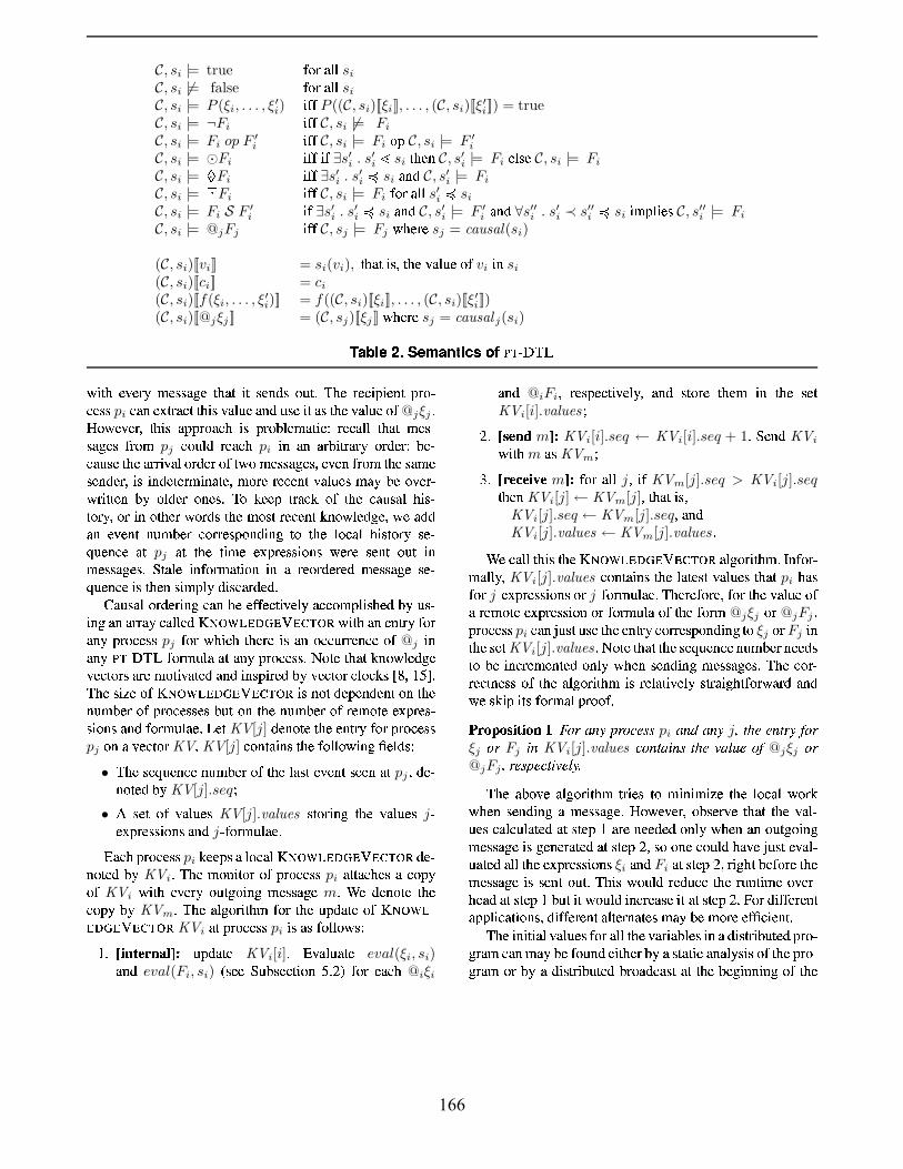
C, si |= trueåVäéaèkôô

si

C, si 6|= falseåeäéaèkôô

si

C, si |= P (ξi, . . . , ξ′i)

ò´åÆåP ((C, si)[[ξi]], . . . , (C, si)[[ξ

′i]]) = true

C, si |= ¬Fi

ò´åÆåC, si 6|= Fi

C, si |= Fi op F ′i

ò´åÆåC, si |= Fi

äóC, si |= F ′

i

C, si |= Fi

ò´åÆåXò¡å∃s′i . s′i

si

æ¡öQêkîC, s′i |= Fi

êkôøë°êC, si |= Fi

C, si |= 0 · Fi

ò´åÆå∃s′i . s′i

si

èPîgñC, s′i |= Fi

C, si |=[

Fi

ò´åÆåC, si |= Fi

åVäéaèkôôs′i

si

C, si |= Fi S F ′i

ò´å∃s′i . s′i

si

èPîgñC, s′i |= F ′

i

èPîgñ∀s′′i . s′i ≺ s′′i

si

òì-óCôò´êëC, s′′i |= Fi

C, si |= @jFj

ò´åÆåC, sj |= Fj

çöQê:éVêsj = causal(si)

(C, si)[[vi]] = si(vi),æöCèPægòøëùæ¡öQê è:ôïQêuäKå

vi

ò¡îsi

(C, si)[[ci]] = ci

(C, si)[[f(ξi, . . . , ξ′i)]] = f((C, si)[[ξi]], . . . , (C, si)[[ξ

′i]])

(C, si)[[@jξj ]] = (C, sj)[[ξj ]]çöQêPé°ê

sj = causal j(si)

$9 & + "+! ¹Kº»o¼s½¾çòæ¡ö`êê:éeû ì!êëëè:úKê$æöCèPæmòæ/ë°êkîQñCë!äïQænþ ½ öQê·é°êkõkòógò¡êkîKæuóKéoä »õkêëë

pi

õèPîêQæéoè:õkææöQòøë èkôïgêEè:îQñïGë°êEò¡æQèjëXæ¡öQê èkôïgêEäKå@jξj

þ6 äçêêPéVùæöQòøë\èóQóKéoäKèkõ:ö òøë·óKéoäðCôêkìèPæ¡ò¡õ#Eé°êkõjèkôôMæ¡ögèPæsì!êë »ëoè:úQêëpå>é°äì

pj

õäïQô¡ñ`éVêè:õköpi

ò¡îÄèPîÁèéeðQò¡æéoèéVûÁäé°ñKê:éðgê »õjèPïGë°êæ¡öQêÀèéeéVòè:ôäé°ñKê:éXäåCæ´çämì!êëëè:úQêëù:êêkîå>éoäìÁæ¡öQêuëèPì!êë°ê:îgñKê:éVùgòÆëmòîgñKêkæ¡ê:éeìò¡îgè:æ¡êùQìäé°êMéVêjõkê:îQæ è:ôïQêëÀìè:û5ðgêäê:é »çméeò¡ææ´ê:î ðgûÖäô¡ñKê:épäîgêëPþ ½ äýKêkê:óÄæéoè:õkýÖäå!æögêdõjè:ïCëè:ô/öQòøë »æ´äéeûùäéò¡îpäæ¡öQê:éçäé°ñgëæ¡öQê/ìäQëVæ)éVêjõkêkîKæ)ýQîgäçô¡êkñQúKêùçêèkñKñèPîÖêKê:îKæsîKïQì-ðgê:épõjäéné°êëVóCäîQñò¡îQú æøäÁæ¡öQê ô´äõjèkôsöKòÆëVæøäéVûüë°ê » ïQêkîQõjê è:æ

pj

èPæÂæögê æò¡ì!êêKóKé°êëë°ò´äîCë\çêPé°êÄë°êkîKæÂäïKæ!ò¡îì!êëëè:úQêëþuãGæ´èkôêdòîgåeäéeìè:æòøäî òî èUé°êjäé°ñKê:éVêjñ ì!êëëè:úQê`ë°ê » ïQêkîQõjêEòøë*æ¡öQê:î-ëVò¡ì-ógôûMñòÆë°õèé°ñKêjñ0þO è:ïCëè:ôaäé°ñKêPéVò¡îQúõjè:î!ðCêêkå>ånêjõ:æ¡òêkôû!è:õjõjäì-óCôòÆëVögêkñsðgûïCë »òîgúè:îèéeé°è:û/õjèkôô¡êkñ ÉÊË7ÌÂÍGÎGÏÐ<ÎGÑ-Î0Ò)ºGË*Ó çò¡æ¡öèPî/ê:îQæéVûåeäéèPîû5óQé°äKõkêëë

pj

åVäéçöKò´õ:ö·æ¡öQêPé°êòÆë/è:î\äõjõ:ïéeé°ê:îQõjêäå@j

ò¡îèPîû ¹º»°¼-½¾ åVäéVìïQô´è/è:æWè:îûóQé°äKõkêëëþ 1 äæ¡êæöCèPæ7ýKîCäçôêjñKúKêêkõkæ´äéoëWèPéVêìäæ¡òè:æ¡êjñèPîgñ/ò¡îCëeógòé°êkñ/ðQû êkõkæ´äé7õkô´äõkýCë 8 FKùJ:H;oþ½ öQêëVòkê/äKå ÉMÊË7ÌpÍGÎGÏÐ<ÎGÑ-Î0ÒXºGË<Ó òøëîCäæ0ñKê:ógêkîQñKêkîKæGäî-æ¡öQêîKïKì-ðCêPéäåóKéoäõjêëëoêëðïKæ*äîÂæ¡öQêMîKïQì-ðgêPéÀäåé°ê:ìäæ¡êMêóQéVêë »ëVòøäîCëèPîgñMåVäéVìïQô´è:êKþ ¾ ê:æ

KV[j]ñKêkîgäæ´êÀæ¡öQêmê:îQæéVû-åeäéXóQé°äKõkêëë

pj

äî-è êjõ:æøäéKV

þKV[j]

õjäîQæ´è:òîGë7æ¡öQêuåVäô¡ô´äçòîgú÷Gêkô¡ñg땽 öQêëoê KïQê:îgõkêmîKïQì-ðgê:éäå<æ¡öQêô´èjë°æ7êKê:îKæaë°êkêkîèPæ

pj

ùQñKê »îgäæ¡êjñðQûKV[j].seq

*•Ø ëoê:æMäKå è:ôïQêë

KV[j].valuesëVæøäéVò¡îQú æögê è:ôïQêë

j»êóQéVêëë°ò´äîCëaèPîgñ

j» åeäéeìïgô¡èkêþ

Yè:õ:öóKéoäõjêëëpi

ýKêkê:óGëXèô´äõè:ô ÉÊË7ÌÂÍGÎGÏÐ<ÎGÑ-Î0Ò)ºGË*Ó ñKê »îgäæ´êkñðQûKVi

þ ½ ögêMìäîKò¡æ´äéuäåóKéoäõjêëëpi

èPæ¡æøè:õ:ögêëè-õäóKûäå

KVi

çò¡æö êêPéVûdäïQæ¡úgäò¡îQúUì!êëëoèkúKêmþ\ê\ñKê:îCäæ´ê·æ¡öQê

õjäóQûÂðgûKVm

þ ½ ögê!è:ô¡úQäéVò¡æöQì åVäéuæ¡öQê!ïógñgèPæ´êäå ÉMÊË7ÌÂÍ)»ÎGÏÐ*ÎGÑ-Î0Ò)ºGË<Ó

KVi

èPægóKéoäõjêëëpi

òøëèjë*åVäô¡ô¡äçëþ ïKógñQè:æ¡ê

KVi[i]þ Y*èkôïCèPæ´ê

eval(ξi, si)èPîgñeval(Fi, si)

(eë°êkêUãCïð0ë°êjõ:æ¡ò´äîM:Gþ I ) åVäé-êjè:õkö@iξi

èPîgñ@iFi

ùMé°êëVógêkõkæò êkôûùsè:îQñ&ë°æ´äéVêÄæögê:ì ò¡î&æögêüë°êkæKVi[i].values

*I)þ

m

KVi[i].seq ← KVi[i].seq + 1þCãGê:îgñ

KViçò¡æömèë

KVm

*Gþ

m<åeäémè:ô¡ô

jù)ò´å

KVm[j].seq > KVi[j].seqæ¡öQê:îKVi[j]← KVm[j]

ùæöCèPægòøëùKVi[j].seq ← KVm[j].seq

ùè:îQñKVi[j].values ← KVm[j].values

þ\êuõè:ô¡ôæöQòøëaæögê ÉMÊË7ÌpÍGÎGÏÐ<ÎGÑ-Î0ÒXºGË<Ó è:ô¡úQäéVò¡æöQì·þeîQåVäé »ìè:ô¡ôûù

KVi[j].valuesõäîKæøèPò¡îCëæögêMô´èPæ´êë°æè:ôïQêëæöCèPæ

pi

öCèjëåeäé

j» êóQéVêëë°ò´äîCëWäé

j» åVäéVìïQô´è:êKþ ½ öQê:éVêjåeäéVêùjåeäé7æ¡öQê"è:ôïQêäKåèéVêkìäæ´êêóQéVêëëVòøäîäéåeäéeìïgô¡èmäåWæ¡öQêåVäéVì

@jξj

äé@jFj

ùóKéoäõjêëë

pi

õjè:î KoïCë°æïCëoê*æ¡öQêê:îQæéVûõäéeéVêëeóCäîQñKòîgúEæ´äξj

äéFj

òîæögêEëoê:æ

KVi[j].valuesþ 1 äæ´ê*æ¡ögè:ææögêEëoê ïgê:îgõkêWîQïKì-ðgê:éQîgêkêkñCë

æ´ä5ðgê-ò¡îQõPé°ê:ì!êkîKæ´êkñ·äîgôûçögê:î\ëoê:îQñKòîgú5ì!êëëoè:úQêëPþ ½ öQêõjäé »éVêjõ:æ¡îQêëëäKåuæ¡öQêèkôúgäéVòæ¡öKì òÆëé°êkô´èPæ¡òêjôû\ë°æéoèPò´úöQæ¡åVäé°çèé°ñèPîQñçêmë°ýKòóMò¡æøëåVäéVìè:ôóQé°äQäåþ "! #$# "&% Õg¥gK³­*>¥Qk:

pi

KKK³j¿a ©gPC ¡>³*j¥g

ξj

¥CFj

¦KVi[j].values

:¥C ¦G«Qs ©Q²:C¢¡¬¥n@jξj

¥g@jFj

¿Gn:´­*kk ´²jj¢ ³:µ½ öQêèPðCäê5è:ô¡úQäéeò¡æ¡öKì'æéeò´êë-æ´äUìò¡îKò¡ìòjêpæögê·ô¡äKõjè:ôuçäéeý

çöQêkî@ëoê:îgñò¡îQúèpì!êëëè:úQêþ 6 äçêêPéVù<äðGëoêPé!êÂæöCèPæÀæ¡öQê è:ô »ïQêëEõjèkôõkïQô´èPæ´êkñè:æWë°æ¡ê:ó /èPéVêîgêkêjñKêkñ!äîQôû!çöQêkîÂèPîÂäïKæ´úQäòîgúì!êëëoè:úQêuòÆëúKêkîQêPéoèPæ´êkñMèPæXëVæ´êPó IGùëoäsäîgêõäïgôñögèê K°ïGëVæ0êèkô »ïgè:æ¡êjñ/è:ô¡ôæögêÀêKóKé°êëë°ò´äîCë

ξi

èPîQñFi

è:ægëVæ´êPó ICùPéeò´úöQæðgêjåeäéVêæ¡öQêì!êëëoè:úQê-òøëMë°êkîKæäïKæeþ ½ öKòÆëçäïgôñpé°êkñKïQõjê-æögê-éeïQîKæ¡òì!êäKêPé »öQêè:ñ/èPæGëVæ´êPó ðïQæò¡ægçäïgôñmò¡îQõ:éVêèjë°êEò¡æGèPæCë°æ¡ê:ó%I0þ)äéXñò´åÆåeêPé°ê:îKæèóQógôò¡õèPæ¡ò´äîCëùjñKò¡å>ånê:éVêkîKæQèkôæ´êPéVîgè:æ¡êëaìèPûðgêuìäé°êÀêkå>÷0õ:ò´ê:îKæeþ½ öQêòîQòæ¡òøè:ô è:ôïQêëGåVäé)è:ô¡ôæögê èPéeòøèðCôêëCò¡îèñòÆëVæéeòðïKæ´êkñÀóKéoä »úéoèPìÄõèPîmìèPûðgêEåVäïKîgñuêkòæ¡öQê:égðgû/èEë°æ´è:æò´õèPîCè:ôûCëVòÆë7äågæ¡öQêóKéoä »úéoèPì äéEðQûèsñòÆëVæéeòðïKæ´êkñðKéoäKèkñKõjèëVæ<èPæWæ¡öQêMðCê:úò¡îKîQòîgúäåEæ¡öQê

166

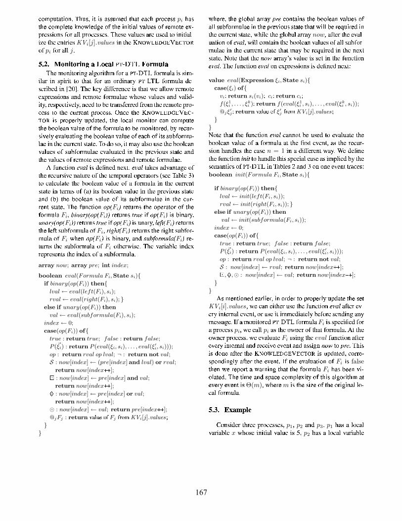
õjäì-ógïKæøèPæ¡ò´äî)þ ½ öQïCëùCò¡æ*òÆëèjëëVïKì!êjñpæöCèPæ*êè:õ:öpóQé°äKõkêëëpi

öCèjëæögê/õjäì-ógô¡ê:æ´êýKîgäçô¡êkñQúKêäå*æögêòîQòæ¡òøè:ô è:ôïQêëEäKåWé°ê:ìäæ¡êê »óKé°êëë°ò´äîCë<åeäéWèkôôgóQé°äKõkêëë°êëþ ½ ögêëoê"èkôïgêë<èPéVêïCëoêkñMæ´äò¡îKò¡æòøè:ô »òjêÀæ¡öQêuêkîKæéeò´êë

KVi[j].valuesò¡îæ¡öQê ÉMÊË7ÌÂÍGÎGÏÐ<ÎGÑ-Î0ÒXºCË*Óäå

pi

åeäéaè:ô¡ôjþ

0 3 <3>= 8 3$ ' 3>=?' ½ öQêÀìäîKò¡æ´äéeò¡îQúèkôúgäéVòæ¡öKì åVäéaè ¹º»°¼-½¾ åeäéeìïgô¡èòøëëVò¡ì »ò¡ô´èéò¡î ëVóQòéeò¡æuæøäUæöCèPæmåeäésèPîdäéVñKòîCèéVû ¹º»°¾)½¾ åeäéeìïgô¡èpñKê »ë°õPéVòðgêkñsò¡î+8>I?R<;oþ ½ ögêýKêPûñò´åÆåeêPé°ê:îgõkêòøëæ¡ögè:æ)çê/è:ô¡ô´äçÁé°ê:ìäæ¡êêóQéVêëëVòøäîGëuè:îQñÂé°ê:ìäæ´ê-åeäéeìïgô¡èkêMçöCäQëoê è:ôïQêëmè:îQñè:ôò´ñ »òæ¡ûùéVêëeógêjõ:æ¡òêjôûùîQêjêkñæ´äðCêæéoèPîGë°åeêPéeéVêjñå>é°äìÁæ¡öQêéVêkìäæ´êóKéoä »õkêëëæ´ä$æögêÂõkïéeéVêkîKæóKéoäõjêëëPþ %mîgõkêÂæögê ÉÊË7ÌÂÍGÎGÏÐ<ÎGÑ-Î0Ò7»

ºGË<Ó òÆësóQé°äógêPé°ôûUïKógñgèPæ´êkñCù<æ¡öQêô´äõè:ôuìäîKò¡æøäéõjè:îdõjäì-óQïQæ¡êæögêðCäQäô¡êjè:îè:ôïQêuäKå)æ¡öQêmåVäéVìïQô´èæ´ä/ðgêuìäîKò¡æøäé°êkñCùPðgû/é°êkõ:ïKé »ëVòêjôû/êèkôïCèPæ¡òîgúmæögêEðCäQäô¡êjèPî èkôïgêuäå0êè:õköMäåGò¡æÆë*ëVïKðgåVäéVìï »ô¡èkêEòîæ¡öQêõ:ïKéné°ê:îQæKëVæøèPæ´êþ ½ äñQä/ëoäCùò¡æKìè:û/è:ôøëoämïCëoêEæögêðCäKäKôêèPîè:ôïQêëäKåmë°ïðgåVäéVìïQô´è:ê-êèkôïCèPæ´êkñ5ò¡îæögêóQéVêKò´äïCëëVæøèPæ´êÂè:îQñæögê è:ôïQêë<äKåGé°ê:ìäæ´êuêóKé°êëëVòøäîGëWèPîgñéVêkìäæ´êuåVäéVìïQô´è:êKþØ ånïKîgõ:æ¡ò´äî P²:G¢ òÆëñKê÷CîQêjñ-îQêQænþ :²:C¢ æ´è:ýKêëuè:ñ è:îKæøè:úQêäKåæögêÀé°êkõkïéëVòêuîgè:æïKéVêäå7æ¡öQêmæ¡êkì-óCäé°èkôgäógêPéoèPæøäéë*(eë°êjê ½ èPðgô¡ê )æ´ä·õè:ô¡õ:ïgô¡è:æ¡êæ¡öQêðCäKäKôêèPîè:ôïQêÂäåè!åeäéeìïgô¡èsò¡îæ¡öQê!õkïéeéVêkîKæ

ëVæøèPæ´êò¡îæ´êPéVìÂëÀäKå (nè ) ò¡æøëðCäQäô¡êjèPî è:ôïQêò¡îÂæ¡öQê/óKé°êòøäïGëÀëVæøèPæ´êèPîQñ (øð ) æögê5ðCäQäô¡êjè:î è:ôïQê$äKå/ò¡æøëÂëVïðCåeäéeìïgô¡èkêpòî`æögêõ:ïKé »éVêkîKæë°æ´è:æ¡êKþ ½ öQêånïKîgõ:æ¡ò´äî ¥­Fi é°ê:æ¡ïéVîCëæ¡öQêäógêPéoèPæøäéuäKåÀæ¡öQêåeäéeìïgô¡è

Fi

ù C«QCƳ>¥­Fi é°ê:æ¡ïéVîCë ´¬K ò´å ¥­ Fi òøëEðQò¡îgèPéeûù¬KGƳ>¥­

Fi é°ê:æ¡ïéVîCë ´¬ ò´å ¥­ Fi òøë)ïQîgèéVûù ¢ Fi é°ê:æ¡ïéVîCëæögêÀôêjå>æ0ëVïKðgåVäéVìïQô´èäåFi

ù «§g©g Fi éVêkæïKéeîGë7æögêéVò¡úKöKæGëVïðCåeäé »ìïQô´èMäKå

Fi

çöQêkî ¥­Fi òøëuðgòîCèéVûùgèPîgñ P¬ek¥CV¤M¬K¢¦ Fi éVê »æïKéeîGëæ¡öQê·ëVïðCåeäéeìïgô¡èäå

Fi

äæögêPé°çòøëoêþ ½ ögê èPéeòøèðCôêòîgñKêéVê:óKé°êë°êkîKæÆë7æ¡öQêÀò¡îQñQêMäKå7èëVïKðgåVäéVìïQô´èþarray now; array pre; int index;

boolean eval(Formula Fi,State si)

if binary(op(Fi)) then

lval← eval(left(Fi), si);

rval← eval(right(Fi), si);

else if unary(op(Fi)) then

val← eval(subformula(Fi), si);

index← 0;

case(op(Fi)) of

true : return true; false : return false;

P (~ξi) : return P (eval(ξi, si), . . . , eval(ξ′i, si)));

op : return rval op lval; ¬ : return not val;

S : now[index]← (pre[index] and lval) or rval;

return now[index ];W : now[index]← pre[index] and val;

return now[index ];V · : now[index]← pre[index] or val;

return now[index ]; : now[index]← val; return pre[index ];@jFj : return FS?T X I Fj H0I Y KVi[j].values

çöQê:éVêùQæögêMúQô¡äðCèkô7èPénéoèPû ­*e õäîQæ´è:òîGëEæ¡öQêðCäKäKôêèPî èkôïgêëuäåè:ô¡ôgë°ïðgåVäéVìïQô´è:êò¡î/æ¡öQêEóQéVêKò´äïCëaëVæøèPæ´êÀæ¡ögè:æQçò´ôôKðgêEé°ê KïKòéVêjñmòîæögêuõkïéeéVêkîKæCë°æ´è:æ¡êùçöKò´ô¡êuæ¡öQêúKô´äðCèkôQèPénéoèPûnow

ùKè:ånæ´êPéaæögêuêè:ô »ïgè:æòøäîäKå P²kC¢ ù:çò´ô¡ôQõäîKæøèPò¡îæ¡öQêEðGäKäô¡êjè:î è:ôïQêë<äåXèkôôCëVïKðgåVäé »ìïQô´è:êò¡îpæögêõ:ïKéné°ê:îQæ7ëVæøèPæ´êMæöCèPæ7ìèPû!ðCêé°ê KïKòéVêjñ-òîpæögê/îgêKæëVæøèPæ´êþ 1 äæ¡ê/æöCèPæ7æögê Q¥K¸ èéeé°è:û ¦ë è:ôïQêòÆëuëoê:æaò¡î!æögêånïKîgõ:æ¡ò´äîP²:G¢ þ ½ öQêuånïKîgõ:æ¡ò´äî P²kC¢ äîêKóKé°êëëVòøäîCëaòøë*ñKê÷CîQêjñ/îQêKæ value eval(Expression ξi,State si)

case(ξi) of

vi return si(vi) ci return ci f(ξ1

i , . . . , ξki ) return f(eval(ξ1

i , si), . . . , eval(ξki , si))

@jξ′

j return FS?T X I ξ′j H0IJY KVi[j].values

1 äæ´êsæöCèPæWæ¡öQê-å>ïQîQõkæòøäî P²:G¢ õjè:îKîgäæ7ðgêsïCëoêkñpæ´äpêèkôïCèPæ´êæ¡öQêðCäQäô¡êjèPî è:ôïQêäåÀèsåVäéVìïQô´èMè:æWæögê÷géoë°æ*êêkîKæ>ùGèjëæ¡öQêMé°êkõkïé »ëVòøäîÂögèPîgñKô¡êëæögêMõèjë°ên = 1

ò¡î5èMñò´åÆåeêPé°ê:îQæXçèPûQþ\ê-ñKê÷CîQêæögêEå>ïQîQõ:æ¡òøäî ¦C æøäögèPîgñKô¡ê*æ¡öKòÆëWëeóCêkõkò´èkôõjèjëoêèjë)òì-óCôò´êkñðgûæ¡öQêë°êkìèPîKæ¡ò´õëaäå ¹º»°¼-½¾ ò¡î ½ èðCôêëIèPîgñ äîäîQêêêkîKææé°èkõkêëboolean init(Formula Fi,State si)

if binary(op(Fi)) then

lval← init(left(Fi, si));

rval← init(right(Fi, si));

else if unary(op(Fi)) then

val← init(subformula(Fi, si));

index← 0;

case(op(Fi)) of

true : return true; false : return false;

P (~ξi) : return P (eval(ξi, si), . . . , eval(ξ′i, si)));

op : return rval op lval; ¬ : return not val;

S : now[index]← rval; return now[index ];W , V · , : now[index]← val; return now[index ];

Ø ë<ì!êkîKæ¡ò´äîQêjñêjèPéVôò´êPéVùjò¡î-äéVñQêPéaæ´äóQé°äógêPé°ôû/ïóCñQèPæ´êÀæ¡öQêë°êkæKVi[i].values

ùçêmõjè:îMê:ò¡æ¡öQêPé7ïCëoêuæ¡öQêå>ïQîQõ:æ¡òøäî P²kC¢ è:ånæ¡ê:éaê »êPéVû/ò¡îKæ´êPéVîgè:ôQêê:îQæÆùjäé7ïGë°êò¡æCòìì!êjñòøèPæ´êkôûðgêkåVäé°êuë°êkîQñKòîgúèPîûì!êëëoè:úQêþeå0èìäîQòæøäé°êkñ ¹º»°¼-½¾ åVäéVìïQô´è

Fi

òÆëWëeógêjõ:òø÷GêkñåVäéèEóQé°äKõkêëë

pi

ùçêõjèkôôpi

èjë<æ¡öQêäçîgêPéWäåXæöCèPæCåeäéeìïgô¡èþ Ø æCæ¡öQêäçîQê:é0óKéoäõjêëëùjçêuêèkôïCèPæ´êFi

ïCë°òîgúæ¡öQêeval

å>ïQîQõ:æ¡òøäî/è:ånæ¡ê:éêêPéVûòîQæ¡ê:éeîCè:ôKè:îQñé°êkõjê:òKêêê:îQæQèPîgñ/èjëë°ò¡úKî Q¥K¸ æ´ä ­e þ ½ öQòøëòøëñgäîQê-è:ånæ´êPéæögê ÉMÊË7ÌÂÍGÎGÏÐ<ÎGÑ-Î0ÒXºCË*Ó òÆëïóCñQèPæ´êkñGùQõjäéné°ê »ëeóGäîQñKòîgúKôûpèkå>æ´êPéuæ¡öQêêKê:îKæeþeåæ¡öQêêèkôïCèPæ¡ò´äî5äKå

Fi

òøëfalseæögê:îpçêé°êPóGäéVæaèMçèéVîKò¡îQúæöCèPæaæögêMåVäéVìïQô´è

Fi

ögèëEðCêkêkî ò »äô´èPæ´êkñ)þ ½ öQêæ¡òì!êè:îQñÂëVóCèkõkê/õäì-ógô¡êQòæ¡û-äKå<æ¡öKòÆëè:ô¡úQäéeò¡æ¡öKì"èPæêêPéVûêêkîKæQòøë

Θ(m)ùçögêPé°ê

mòøë*æ¡öQêëVòkêäåXæögêäéVò´úò¡îgè:ôQô¡ä »õjèkôQåVäéVìïQô´èþ

0 ! " $&%'

O äîCë°ò¡ñQêPéÀæ¡öé°êkêMóKéoäõjêëë°êëùp1ùp2è:îQñ

p3þp1ögèjëmè-ô´äõè:ô

èéVò´èPðgô¡êxçöCäQë°êsò¡îKò¡æòøè:ôèkôïgêòÆë :gù

p2öCèjëmèsô¡äKõjè:ôèPéeòøèðCôê

167

C, si |= 0 · Fi = C, si |= Fi

äé*(∃s′i . s′i

si

èPîgñC, s′i |= 0 · Fi

)

C, si |=[

Fi = C, si |= Fi

èPîgñ (∃s′i . s′i

si

ò¡ì-ógôò¡êëC, s′i |=

[Fi

)

C, si |= FiSF ′i = C, si |= F ′

i

äé(C, si |= Fi

è:îQñ∃s′i . s′i

si

èPîgñC, s′i |= FiSF ′

i )

$9 & P*" + " ! ¹º»°¼-½¾

yçòæ¡öÂò¡îKò¡æ¡ò´èkôè:ôïQê%=5èPîgñ

p2ìäîKò¡æøäéëæögê-åeäéeìïgô¡è [

(y ≥@1x)

þ Ø îsêgè:ì-ógô¡êÀõjäì-óQïKæøèPæ¡òøäîòøëEë°ögäçî/ò¡î0ò´úïKéVê Cþ

p3

p2

p1

0

5

0

5

0

5

2

6

2

6

2

6

2

6

2

6

0

9

1

9

2

6

e20 e21 e22 e23

e30 e31 e32

e10 e11

e12

e13

e14

x=5

y=7

x=9

y=3

1

6

x=6

(violation)

KV[1].seq

KV[1].values

)+ Q+ ! [(y ≥ @1x)

p2

½ öQêPé°êòøë7äîgôûäîgêåVäéVìïQô´èWæøäÀìäîKò¡æ´äéCçò¡æ¡öèë°òîgúKô¡êäKõkõ:ïKé »éVêkîQõkê/äKåè:î@äóCêPéoèPæøäéVùîgèPì!êjôû

@1xþ 6 ê:îQõjêùKæ¡öQê ÉMÊË7ÌÂÍ)»

ÎGÏÐ*ÎGÑ-Î0Ò)ºGË<Ó öCèjëEèë°òîgúKô¡êê:îKæéVû-çöQò¡õköõjäéeé°êëeóGäîgñgë<æ´äp1þ

ÿ äéVêäê:éVùGëVò¡îQõjêæögêäîgôû5é°ê:ìäæ¡êêóKé°êëëVòøäî·æøäpðgê!æéoè:õkýKêkñòøë

xùKV[1].values

ë°òì-óCôû!ëVæøäé°êë*æ¡öQêè:ôïQêäåxþeî-æögê÷Gú »ïé°êùQîgêKæaæøäÂêè:õköpêêkîKæ>ùCçê!ëVöCäç

KV[1]è:æWæöCèPæWò¡îCëVæøèPîQæWåeäé

æöCèPæaóKéoäõjêëëþKV[1]

òÆëmúéoèóQöQò¡õè:ô¡ôû5ñòÆëeóCô¡è:ûQêjñ!ðgû·è!ë°æ´èkõ:ý$äKåæ¡çäÂîKïQì-ðgêPéëùgæögêMæøäó·îQïKì-ðgê:éÀë°ögäçò¡îQú

KV[1].seqèPîgñpæögê

ðCäæ¡æøäì îKïQì-ðgêPéWëVögäçò¡îQú/æögê è:ôïQêåeäéxþ

½ öQê õjäì-ógïKæøèPæ¡ò´äîüëVæøèéVæÆë$äKåÆå5çòæ¡öÖæ¡öQê`ò¡îKò¡æòøè:ô è:ôïQêë$äKåx = 5

èPîgñy = 7

þ Ø ô¡ôEóKéoäõjêëëoêëýKîCäç æ¡öQêpò¡îKò¡æòøè:ô èkôïgêäå

xùögê:îgõkêÀæ¡öQê

KV[1].valuesåeäéaêè:õkö/óKéoäõjêëëaögèë èkôïgê#:0þ

næWòÆëêjèëVû·æøäë°êjê-æöCèPæ<æ¡öQêsìäîQòæøäé°êkñpåVäéVìïQô´è5[(y ≥ @1x)ögäô¡ñgëWòîQòæ¡òøè:ô¡ôûèPæ

p2þãGïðGëoê KïQê:îQæ¡ôûùjè:æ

p1æögêPé°êuòÆëèPîsòîQæ¡ê:éeîCè:ô

êê:îQæe11

çöQò¡õköëoê:æÆëx = 9

èPîgñuïKógñgèPæ´êëKV1[1].values

õäé »éVêëeóCäîQñKòîgúKôûKþ CGé°äKõkêëëp1æögê:î-ëoê:îgñgëèÀì!êëëoèkúKêæ´ä

p2çò¡æöè

õjäóQûäåXòæÆëWõkïéeéVêkîKæKV

þ Ø îgäæögêPé)ò¡îKæ´êPéVîgèkôKêêkîKæe13

õèPïGë°êëxæ´äsðCêsëoê:æaæ´ä AGþBCGéoäõjêëë

p1è:úgèPò¡îpë°êkîQñgëuèì!êëëoèkúKêùKæöQòøëÀæò¡ì!ê

æ´äp3ùçòæ¡ösæögêuïKógñQè:æ¡êjñ

KVþ4CGé°äKõkêëë

p3ïóCñQèPæ´êëWòæÆë

KVèPîgñë°ê:îgñgëWæöQòøë*äîæ¡öQêuì!êëëoè:úQêÀò¡æ)ë°ê:îgñgë<æ´ä

p2þ

Ø æ0óKéoäõkêëëp2ùæögêì!êëëè:úQêë°ê:îQæGðQû

p3ögèóQógêkîCë<æ´äèPénéVòê

êjèé°ôò¡ê:éÀæöCèPî5æögê-ì!êëëoè:úQêåÆéoäìp1þ ½ öQêPé°êkåVäé°êùGèPæêKê:îKæ

e21ù

äîéVêjõkê:ò ò¡îQú/æ¡öQêì!êëëoèkúKêmåÆéoäìp3ùjóQé°äKõkêëë

p2òøëèPðgô¡êuæøä/ïKó »ñQè:æ¡êò¡æøë

KVæ´äsæ¡öQê/äîQêë°êkîKæXè:æXêêkîKæ

e14þ ½ ögêìäîKò¡æøäéèPæ

p2è:úgèPò¡î/êè:ôïgèPæ´êëXæ¡öQêóKéoäógê:éeæ¡û/èPîgñ/÷CîQñCë7æöCèPæQòæ0ëVæ¡ò¡ô¡ôQögäô¡ñgëPþ ½ öQêì!êëëoè:úQêë°êkîKæ<ðgûp1÷Cîgèkôôû$èéeéeò êëè:æ

e22ðïKæ*æ¡öQê

KVóQò´ú »úûKðCè:õkýKêkñäîòÆëò´úîCäé°êkñ!èjëòæaöCèjëÀèsëVìèkôô¡êPé

KV[1].seqæöCèPî

KV2[1].seqþ ½ ögêìäîQòæøäéaõjäéné°êkõkæ¡ôûõjäîKæ¡òîQïQêë7æ´äñKêjõkô´èé°êæögêóKéoäóCêPéVæûè:ôò¡ñ)þ 6 äçêêPéVù:èPîgäæögêPé0ò¡îKæ´êPéVîgèkôêê:îQæQèPæ

p2õèPïCëoêë

æögêèkôïgêäåyæøä!ñé°äó!æ´ä

3ùCè:æ7çöQò¡õköóCäòîQæ)æ¡öQê/ìäîKò¡æ´äéñKê »æ¡êjõ:æÆë*èóKéoäóCêPéVæû Kò´äKô¡è:æòøäîXþ

Û /5,4 [F /ußWß98\êögèê\ò¡ì-ógô¡ê:ì!ê:îQæ¡êjñ@æ¡öQêèðGäêæ´êkõköKîQò KïQê\èë5è\æ´äQäôÆù

õjèkôô¡êkñ ¼-×ÆØ-ÊWÙ ( ¼-× ëVæéeòðïKæ´êkñ Ø-ÊWÙ ôûCë°òøë ) (eë°êkê )ò¡úKïé°ê ) þ ¼-×n»Ø-ÊWÙ òøë-óQïKðgôò¡õjôûdèè:ò¡ô´èðCôê$è:îQñ@õèPî ðCêñQäçîgô¡äQè:ñQêkñUåÆéoäì !#"%$&"'(*)+,"-.+$0/1/' þ uäæö ¼-×ÆØ-ÊWÙ èPîQñæögêuå>é°è:ì!êPçäéVýïKîQñQêPéaçöKò´õ:ö/ò¡æ0äógê:é°è:æ¡êë<èPéVêçméeò¡ææ´ê:îMòî S èèþ2 43 <3>=?

Ø îQïKì-ðgê:éGäKåGåeäéeìèkôòÆëVìÂë)õjè:îmðgêïCëoêkñmæ´äué°êjèëoäî/èPðCäïQæñòÆë »æéVòðïKæ´êkñÂë°ûCëVæ´ê:ìÂëùQæ¡öQê/ìägëVæ7îgè:æïKé°èkôXäîgêðgêkòîgú Ø õ:æøäéëX8/Igù B;oþØ õ:æøäéëèé°ê/èìäñQêkôGäå<ñKòøë°æéVòðïKæ´êkñMéVêè:õkæòKêäðEKêkõkæøëèPîgñ-ögèêèsðïKò´ôæ » òî·îCäæ¡ò´äî$äåê:îQõèó0ëVïQô´èPæ¡òøäîèPîgñ5òîQæ¡ê:é°èkõ:æ¡ò´äîGùGìèPýKò¡îQúæögê:ì çêkô¡ômë°ïKò¡æ¡êjñ æøäé°êPóKé°êëoê:îQæuêäôïKæ¡ò´äî@èPîQñdõjäKäéVñKòîCèPæ¡ò´äîðgêkæ¡çêjê:îò¡îKæ´êPéoè:õ:æ¡ò¡îQúõjäì-óCäîgê:îQæøë0òîMñòÆëVæéeòðïKæ´êkñ/èPóKógôò´õjèPæ¡òøäîCëPþO äîgõkêPógæïCè:ô¡ôûùPè:îMè:õkæ´äé7ê:îgõjèPóGëVïgô¡è:æ¡êëaèuëVæøèPæ´êùèEæöKéVêè:ñ/äKå)õjäî »æéoäôÆùèPîgñè\ë°ê:æäåóQé°äKõkêjñïé°êëçöKò´õ:ö ìè:îKòóQïgô¡è:æ¡êÂæögê\ëVæøèPæ´êþØ õ:æøäéëõäKäé°ñò¡îgè:æ¡êðQûpèëVûQîQõ:öKé°äîgäïCë°ôûë°êkîQñò¡îQú!ì!êëëè:úQêëÀæ´äêjèkõ:öpè:îgäæögêPéVþ&nîpæ¡öQê-è:õ:æøäéå>é°è:ì!êPçäéeý0ùgèñKòøë°æéVòðïKæ´êkñpë°ûCë°æ¡êkìõjäîCëVòÆëVæÆëÂäå-ñò´åÆåeêPé°ê:îKæè:õkæ´äéoë!õjäììïQîKò´õjè:æò¡îQúæ¡öéoäïgúö@ì!êë »ëoèkúKêëPþ ½ öKïGëù0æögêPé°ê-òøë/èPî$è:õkæ´äéåVäéêè:õ:ö5óQé°äKõkêëëò¡î·æögêÂëVûGë »æ¡êkì·þnîsæögêmòì-óCôêkì!ê:îKæøèPæ¡òøäîGùjêè:õköMæ¡ûóCêmäKåaèkõ:æøäé (näéaóKéoäõjêëë ) òÆëñKêkîgäæ´êkñðQû$è S èèõjô¡èëëmæ¡ögè:æ*êKæ´ê:îgñgëmèsðGèjë°êõjô¡èëë5(6>87aþ

½ öKòÆëðGèjëoêõkô´èjëëò¡ì-ógô¡ê:ì!êkîKæÆëèì!êëëè:úKê ïgê:ïQê/è:îQñ!óKéoäò´ñKêëæögêì!ê:æ¡ögäKñ > :9åeäéaèjë°ûKîgõ:öéoäîCäïGëGì!êëëoèkúKêë°ê:îgñò¡îQú)þ Yè:õ:öè:õkæ´äé0äðEKêkõkæêQêkõ:ïQæ¡êëCò¡î/èëoêPóCèPé°è:æ¡êæ¡öé°êjè:ñ)þ ½ ögêEë°æ´è:æ¡êäåGè:îèkõ »æ´äé*òÆëé°êPóKé°êëoê:îQæ¡êjñðgûæögê÷GêjôñCëäå*æögê S èèõjô¡èëëPþBYè:õkö S èèõkô´èjëëWè:ôøëoäõäîQæ´è:òîGëXèë°ê:æCäå;:<%= -6Mì!ê:æ¡ögäKñgë)æ¡ögèPægõjè:îðgêEò¡î »äýKêjñò¡î!é°êëeóGäîGë°ê/æøäì!êëëè:úKêëé°êkõjê:òêjñ!å>é°äì"äæögêPéè:õ:æøäéëþØ ë°ûCëVæ´ê:ì&ôêKêkôGè:õkæ´äé*õjè:ô¡ô¡êkñ Çk ¥g?>$QK§Cj æøèPýKêëèì!êëëoèkúKêèPîgñæéoèPîCëoånê:éoë)ò¡æKæøämæögêì!êëëè:úQê ïQêkïQêäåCæ¡öQêEæøèéVúKêkæKè:õ:æøäéVþ ½ öQêæ´èPéeúQê:æèkõ:æøäéæ´è:ýKêëèPîèèPò´ô¡èPðgô¡ê!ì!êëëoèkúKêå>éoäì æögê!ì!êëëoèkúKê ïgê:ïQêè:îQñpòîäýKêëuæ¡öQê-ì!ê:æ¡ögäKñpì!ê:îKæ¡òøäîQêjñò¡î·æ¡öQê-ì!êëëoèkúKêþ

168

öQò¡ô¡êóKéoäõkêëë°òîgúèì!êëëoè:úQêù:èPîè:õ:æøäé0ìè:ûëoê:îgñuì!êëëoèkúKêë0æøääæ¡öQêPéuèkõ:æøäéëþgÿêëëè:úKê!ëoê:îQñKòîgúCùgðgê:ò¡îQú5èjë°ûKîgõ:öéoäîCäïGëùKîQêKêPéðgô´äõ:ýGë)è:îè:õkæ´äéeþ 6 äçêêPéVùPèPî/è:õkæ´äéGðgô´äõ:ýGë)ò¡åGæ¡öQê:éVêòÆëXîgäì!êë »ëoè:úQêò¡î!òæÆëEì!êëëè:úKê ïQêkïQêKþ ½ ögêMëVûGëVæ´ê:ì òÆëEò¡îKò¡æòøè:ôòjêkñ-ðgû!æ¡öQêÇk ¥g?>$QK§Cj äðEKêkõ:æaæ¡ögè:æaõ:éVêèPæ´êëmè:ô¡ôaæ¡öQê-è:õ:æøäéëÀòîpæögê!ëVûCë »æ¡êkìèPîQñsëVæøèéVæøë<æögêêKêkõkïKæ¡ò´äîäåXæögêmëVûGëVæ´ê:ì·þ2 = <76 23 <3>=? ½ öQêïCëoêPéXäå ¼-×ÆØ-ÊWÙ ëVógêjõ:òø÷Gêë)æ¡öQêô´äõjèkô ¹º»°¼-½¾ åVäéVìïQô´è:êæ´ä!ðgêMìäîQòæøäé°êkñäîÂêè:õ:ö·è:õkæ´äéò¡îèsëVógêjõ:òøè:ôW÷Gô¡êþYè:õköpè:õkæ´äé

ögèjë*èÀïQîKò ïgêîgè:ì!êùjçöKò´õ:öMòøë*æ¡öQêuîgèPì!êmäåXæögêuõäéeéVêëeóCäîQñKòîgúóKéoäõkêëëPþ ½ öQêîgè:ì!êuòÆë<óCèëë°êjñèjëèëVæéeò¡îQú-èPæGæ¡öQêæò¡ì!êõPé°êjè:æòøäîäåXè:î-èkõ:æøäéVþØ ë 0ò¡úKïé°ê ëVögäçëùæ¡öQêõäé°êÁäå ¼s×>ØsÊWÙ õäîCë°òøë°æøëäKåæ¡çäìäKñïQô¡êë*èPî «Q ´¬¤:g g ´¦¥K ìäñïgôêè:îQñ@è ¤/¥KC ¥C°¨

«K§ ìäñKïQô¡êþ ½ öQêòîGëVæéeïQì!ê:îQæ´è:æòøäî-ìäñKïQô¡êæøèPýKêëEæ¡öQêsëVógêjõ:òø÷ »õjèPæ¡òøäî÷Gôê/è:îQñsæ¡öQêñòÆëVæéVòðïQæ¡êjñ/óQé°äKúéoèPì çméVòæ¡æ¡êkîòî-æ¡öQêèðGäêåÆéoèPì!êPçäéVý èPîQñdõPé°êjèPæ´êë!è S èèõkô´èjëë7 >87 :; dæ¡ögè:æòì-óCôêkì!ê:îKæÆëmèô´äõjèkôWìäîQòæøäéuåVäémêjè:õkö$è:õkæ´äé (>äéÀóKéoäõjêëë ) þeæè:ôøëoäèPïQæ´äìèPæ¡ò¡õè:ô¡ôû\òîGëVæéeïQì!ê:îKæÆë/æögêpñKòøë°æéVòðïKæ´êkñ$óKéoäúéoèPì C ©g*³K ¡k:¥KgE¢:²jj¢ (nè:ånæ¡ê:é)õjäì-óQò´ô¡è:æòøäî ) ùëäuæ¡ögè:ææögêEñòÆëVæéeòðïKæ´êkñóKéoäúéoèPì òîäýKêëmò¡æÆë/ô´äõè:ôìäîKò¡æøäéçögê:îQêKêPéuò¡æEìäñòø÷Gêëè÷Gêkô¡ñ èPéeòøèðCôê (Æò¡îKæ´êPéVîgè:ô)êê:îQæ ) ùCë°êkîQñgëuèì!êëëoèkúKêùCäéEòîäýKêëèì!ê:æ¡ögäKñ (øéVêjõkê:ò êÀêêkîKæ ) þ%mîgêìè:û è:ôæ´êPéVîgèPæ´êkôûdõkögäKägë°ê·æøä`êè:ôïgèPæ´ê·æ¡öQê\êPóQòÆëVæ´ê:ìò´õ

êóQéVêëëVòøäîGëè:îQñåVäéVìïQô´è:êÂòìì!êjñòøèPæ´êkôû$ðCêkåVäé°ê5ëoê:îQñKòîgú èPîêê:îQæ(nãCïKðGë°êjõ:æ¡ò´äî9:0þ ) þeî-æöQòøëõèjëoêæ¡öQêô´äõè:ôCìäîKò¡æ´äéaòÆëîgäæòîäýQêkñpçöQê:î$÷0êkô¡ñ èéVò´èPðgô¡êëèPéVê-ìäKñòø÷Gêkñ)þ öKò´ôêéeïQîKæ¡òì!êäêPéVöQêè:ñmçèjëaîCäæQæögêìè Käéaõjäîgõkê:éeîåVäéXïGëaò¡î/ò¡ì-ógô¡ê:ì!ê:îQæò¡îQúäïéuóKéoäæøäæ¡ûógêùCñQêkô´èPûKò¡îQúë°ïQõ:ö\êè:ôïgèPæ¡òøäî·úKêkîQêPéoè:ô¡ôû5éVêjñïQõjêëæögêéVïKîKæ¡ò¡ì!êuäê:éeögêjè:ñ)þ2 ! $ Uê òì-óCôêkì!ê:îKæ´êkñ æögê åVäô¡ô¡äçò¡îQú äæ¡òîgú èkôúgäéVòæ¡öKì pè

póKéoäõkêëëèjë°ýCëåeäé äæ´êsäî5è/éVêëoäKôïQæòøäîpåÆéoäìNäæ »êPéëîCèPì!êkñ7

17

2 7

N

ùWçöQêPé°êN

òÆë·ò¡îKò¡æòøè:ôòkêkñÖæøäÖè:î èPénðgòæé°èPéeûÁðïKæ!÷KêjñóCägëVò¡æò ê@îQïKì »ðgêPéVþ\ê èjëëVïKì!êÄæöCèPæpæögêóQé°äKõkêëë°êë@èé°êÄõäîQîQêkõkæ¡êjñ òî èæé°êkê$ýKò¡îQñdäKåîgê:æ´çäéeý`çòæ¡ödæ¡öQê ÁèPæmæögêéoäKäæmäåMæ¡öQêæé°êkêÁè:îQñ æ¡öQê äæ´êPéëèPæpñò´åÆåeêPé°ê:îKæîCäñQêëþ Yèkõ:ö äæ´êPé$é°è:î »ñQäì!ôûÝñQêkõ:ò´ñKêë ò´ådò¡æ çèPîKæÆëÁæ´ä äæ´êåVäéÁäéÁè:úgèPò¡îCëVæUæ¡öQêéVêëoäôïKæ¡òøäîGùsè:îQñ õjäéeé°êëeóGäîgñò¡îQúKôûëVæøäé°êë Ääé R ò¡î èÖô¡ä »õjè:ô/ë°æ´è:æ¡ê èéVòøèðgô¡êUõjè:ô¡ô¡êkñ!7*þ ½ ögê äæ¡ê:é-æ¡öQêkî ëoê:îQñCëòæÆëñKêkõkòøë°ò´äîæøä ò¡æÆë@ò¡ìì!êkñKò´è:æ¡êÁóCèPéVêkîKæpòî&æögêÄæé°êkêþ ½ öQêÁóCèPé »ê:îKæaõjäKôô¡êkõkæøëæögêäæ¡êëÀèPîgñÂë°êkîQñCëæ¡öQê-ëVïKìÝäKå<ò¡æøë äæ´êMè:îQñòæÆëóKéoäúKêkîKò´êë äæ´êëæ´äòæÆëÀòìì!êjñòøèPæ´êóCèPéVêkîKæeþ ½ öQê póKéoä »õkêëëõäô¡ôêjõ:æÆëè:ô¡ô7æögê äæ´êëuèPîQñéVêKoêjõ:æÆëæögêé°êëäôïKæ¡ò´äîäîQôû!ò´åögè:ô¡åäéìäé°ê äæ´êPéëÀöCèêéVêKoêjõ:æ´êkñ0þ \ê-ìäîQòæøäéEæ¡öQê-åeäKôô´äç »òîgúMëoèkånêkæûóKéoäógê:éeæ¡ûèPæ

reject→ ((∑

i∈[1..N ] @Voteri(vote)) < N/2)

½ öQêóKéoäógê:éeæ¡ûçèjë/åeäïKîQñæ´äpðCê Kò´äKô¡è:æ¡êjñ·òî ë°êê:é°èkôWéVïKîGëaèPæëoäì!ê äæ¡ê:éEîCäñQêëùgæögê äæ¡ê:éuëoê:îQæ7æ¡öQê!ë°ïKì äKåò¡æÆëóQé°äKúKêkîKò´êëäæ´êëuçòæ¡ögäïKæWè:ñQñò¡îQú!ò¡æÆëäçî äæ´êþ ½ öKòÆëEé°êë°ïQôæ¡êjñ!ò¡îÂæ¡öQêé°ê »Koêjõ:æ¡ò´äîäåGæ¡öQêé°êëäôïKæ¡ò´äîçöQê:îò¡æCë°ögäïQô¡ñögèêðCêkê:î/èkõkõkê:óQæ´êkñ)þ\êögèêmè:ôøëoäMæ´êëVæ´êkñ-è êkõkæ´äéaõjô¡äKõ:ý28 FQùJ:H;Wè:ô¡úQäéVò¡æöQìüò¡ì »ógô¡ê:ì!êkîKæ´êkñò¡îæ¡öQêsåÆéoèPì!êPçäéeý-óQéVêë°ê:îQæ¡êjñò¡îÂæ¡öKòÆëuëoêkõ:æ¡òøäî)þ ½ öQêè:ô¡úQäéeò¡æöQì çèjëÀò¡ì-ógô¡ê:ì!ê:îQæ¡êjñèjëóGèéVæ7äKå*úKô´äðGè:ôXë°îgèPóGëVöCäæaèPîQñ

úQèPénðGè:úKê-õäô¡ôêjõ:æ¡ò´äî\è:ô¡úQäéeò¡æöQì·þnî\æöQòøëè:ô¡úQäéVò¡æöQìpù0êè:õkö·óKéoä »õkêëëòÆëèjëëVïKì!êjñpæ´äpöCèêè-ô¡äKõjè:ôKêkõ:æøäéuõjô¡äKõ:ýVæ¡ögèPæWò¡æ*ïKó »ñQè:æ¡êëèkõkõäé°ñò¡îQúæøäÂæögêë°æ´è:îQñgèé°ñ êjõ:æøäéÀõkô´äõký5èkôúgäéVòæ¡öKì 8 FG;

çöQêkîQêê:éuæögêPé°êòÆëè:î$ò¡îKæ´êPéVîgè:ôêê:îQæÆùXè5ë°êkîQñêêkîKæEäé/è-é°ê »õkêkòêêê:îQænþ ½ öQêÀëè:åeê:æ¡ûóQé°äógê:éeæ¡ûuæ¡ögè:ææögêÀè:ô¡úQäéVò¡æöQììïCëVæCëoèPæ »òøëoå>ûMòøë<æ¡ögèPæ>ùèPæGêê:éeû/óKéoäõkêëëpi

<,:èkôôgê:îQæéVò´êë<äKå)æ¡öQêô¡äKõjèkô#êjõ »æ´äéÀõkô´äõ:ýpìïCë°æaðgê-úé°êjè:æ¡ê:éæöCèPî·äéuê KïgèkôXæøäÂæögê-ô¡äKõjè:ôêjõ:æøäéõkô´äõkýò¡î5èMõjè:ïCëoèkôôû5ô¡è:æ¡êëVæ7óKé°êkõjêkñò¡îQúpëVæøèPæ´ê-äKåè:îûpäæögêPéóKéoä »õkêëëù .mêKóKé°êëëoêkñ/èëWæ¡öQêmåeäKôô´äçò¡îQú

i» åVäéVìïQô´è&

[(

∧

j∈[1..n]

V ≥ @jV )

çöQê:éVêV ≥ V ′ çöQêkî$êê:éeûêkîKæéeûò¡î V

òøë/úé°êjè:æ¡ê:éæ¡ögèPîUäéê Kïgè:ôjæøäuæ¡öQêõjäéné°êëVóCäîQñò¡îQúêkîKæéeûòî

V ′ þ Ø îgäæögêPé)ëoè:åeê:æ¡ûóKéoäó »êPéVæû-ëVæøèPæ´êëaæ¡ögè:æ,kèPæCêêPéVûmóKéoäõkêëëpi

æ¡öQêi» æ¡ö/ê:îKæéVû/òîòæÆëWô´äõè:ô

êkõkæ´äéÀõkô´äõ:ýpìïCë°æaðgê!ëVæéVò¡õkæ¡ôûúé°êjè:æ¡ê:éEæ¡ögè:îÂæ¡öQêi» æö5ê:îQæéVû·äåæögêô¡äKõjèkô êjõ:æøäé)õkô´äõkýäå)è:îû/äæ¡öQê:é0óKéoäõjêëë.þ ½ öQòøë7õèPîðgêuê »óKé°êëë°êkñMèjë<æögêåVäô¡ô¡äçò¡îQú

i» åeäéeìïgô¡è

[(

∧

j∈[1..n]

V [i] > @jV [i])

½ öQêÀëoêkõjäîQñóKéoäóCêPéVæûçèjëaåVäïQîQñæ´äðCê òøäô´èPæ´êkñmò¡îMëoäì!êõäì »óQïQæ´è:æòøäîGëmñïQê!æ´äè-ðïQúõèPïCëoêkñ5ðgûånè:ò¡ôïé°êæøä5òîgõPé°ê:ì!êkîKæ<æ¡öQêi» æ¡öpêkîKæéeû·äåæ¡öQê-ô´äõjèkôêkõkæ´äéõjô¡äKõ:ý·äåóKéoäõjêëë

pi

çöQê:îÂé°ê »õkêkòò¡îQú/êKê:îKæÆëþ½ öQêë°êmë°òì-óCôêuêgè:ì-ógô¡êë7ò´ôôïCë°æéoèPæ´êæ¡öQêÀóKéoè:õ:æ¡ò´õjè:ôKïKæ¡ò¡ôò¡æû-èPîQñóCäçê:é0äKå ¹º»°¼-½¾ è:îQñmæ¡öQêìäîQòæøäéVòîgúÀæøäKäKô ¼-×ÆØ-ÊWÙ ðGèjëoêkñäîòæeþ

*Û"!5ßWÞÀ8náâeßWÞWÞà$#/ááÀ % ß<'&½ öKòÆë7çäéVýéVê:óKé°êë°êkîKæÆë)æögêÀ÷géoë°ægëVæ´êPó/ò¡îêjåÆånêjõ:æ¡òêñòÆëVæéeòðïKæ´êkñìäîQòæøäéVòîgú0þ ½ ögêçäéeýMóKé°êëoê:îKæ´êkñMöQê:éVêëVïgúKúQêëVæÆëèuîQïKì-ðCêPé<äåóKéoäðCôêkìÂëgæöCèPæé°ê ïQòé°ê*ånïéVæ¡öQêPéQéVêë°êèé°õ:ö)þ ½ öQêô¡äKúò´õ*ò¡æøëoêkô¡åCõjäïgôñðgêìè:ñQê<ìäé°ê*êóKé°êëëVòKêëoäuæ¡ögèPæò¡æêóQéVêëëoêëCîCäæäîgôûëoèkånêkæûù

ðïKæWè:ôøëoäÂôò ê:îgêëëEóKéoäóCêPéVæò´êëPþ %mîQêñKò¡ån÷Gõ:ïgôæ¡ûòÆëæ¡ögè:æWëäånæ¡çèPéVêñKêêjô¡äógê:éoëuèé°êséVêjôïgõ:æøèPîKæWæøäpïCëoêåeäéeìèkôaîgäæ´è:æòøäîGëþ Ø óCèPéeæ¡òøè:ôëoäKôïQæòøäî ìè:ûðgê·æøäì!êPéVúKêpæ¡öQê5óQéVêë°ê:îQæuçäéVý@çòæ¡ö`è5ìäéVêêóQéVêëë°òê5èPîQñ\óQé°äKúéoèPìì!êPéåÆéVò´ê:îQñQôûUìäîQòæøäéVò¡îQúæ´ê:ì-óGäéoè:ôô¡äKúò´õ\ëVïgõ:ö`èë Y ÙWÐ<ÍGÎ 8/A<;þ Ø õäì-ógô¡ê:ì!êkîKæøèéVû@èóKóQé°äQè:õköUòÆëæ´äñKêêjô¡äóòÆëVïCè:ôgîgäæ´è:æòøäîGëWèPîgñsëVûQîKæ¡öQêëVò:ò¡îQúæ´ê:ì-óGäéoè:ôô´äúKò¡õåeäéeìïgô¡èëaå>é°äì ë°ïQõköîgäæ´è:æòøäîGëþ ½ ögêPé°êÀìèPûsè:ôøëoä/ðgêÀæ¡öQêÀóCägëëVò »ðQò´ôò¡æ¡ûpäåEô¡êjèPéeîQòîgú!åeäéeìïgô¡èëðGèjë°êjñÂäîé°êPóQéVêë°ê:îQæ´è:æò êë°õjê:îgèPé »ò´ägëþØ îíò¡îKæ´êPé°êë°æò¡îQú èê:îQïQêäKå å>ïQæïKéVêªò¡îêë°æò´úQè:æòøäî æöCèPæ

äïKéÖçäéVýëVïQúQúKêëVæÆëÖòøë çögèPæ`çê õjèkôô)( Q¥¸¢PK§gj¨>Q:

169

ÇÀ´­*kk ´¨Pg ¡PE>¥§0eK¤¤M¦§ þ É îCäçôêjñKúKê » ðGèjëoêkñ Ø ëeógêjõ:æ »%éeò´ê:îQæ¡êjñ CGéoäúé°è:ììòîgúòÆë-èpì!ê:æøè » óKéoäúé°è:ììòîgú·ñòÆë°õ:òógôò¡îQêæöCèPæsòøëëVïQòæøèðCôê åVäé·ñòÆëVæéeòðïKæ´êkñüèóKóCôò´õjè:æòøäîGëþ eîÖæ¡öKòÆë·óKéoä »úéoèPììò¡îQú óGèéoè:ñò´úìpùèóKóQé°äóKéVò´è:æ¡êüè:õkæòøäîGëdèPéVê èjëëoäKõ:òøèPæ´êkñçòæ¡ö êè:õkö ëoèkånêkæû åVäéVìïQô´è<*<æ¡öQêë°êè:õkæòøäîGëèPéVê$æ´è:ýKê:î çöQêkî »êêPé7æögêuåVäéVìïQô´èEòøë*òøäô´èPæ´êkñæ´äúïQò¡ñQêÀæ¡öQêóQé°äKúéoèPì èPîgñMèäò´ñõjèPæøèjë°æéoäógöKò´õånè:ò¡ôïé°êëPþU'&Þß 8*gà ; 1CÞ½ öQêU÷géoë°æ/æ¡öé°êkê\è:ïKæ¡ögäéoëÂèé°êë°ïóQóCäéVæ´êkñ ò¡î óCèéVæmðQû`æögê ¼ ê »ånêkîCë°ê Ø ñ#èPîQõjêkñ Àêëoêjèé°õ:ö C0é°ä Koêjõ:æÆë Ø úKê:îgõPû (øæ¡öQê ¼Ø -C Ø C ½ % ½gØ ã É CGéoäúé°è:ìpùõjäîQæéoè:õkæ <R?AHRHI » RHR » I » R:F<AQùMæ¡öQê¼uØ -C Ø U % 1 Yã ½ CGéoäúéoèPìpù@õjäîKæé°èkõ:æ \<A J: » R » OÀ»EWHR?= ) ù*æögê % 1 (éoèPîQæ 1 RHRHRLN » R?I » » RH= J:gùWè:îQñ`æögêUÿ ä »æ´äé°äKô¡è (éoèPîQæ/ÿ % ½ % % ¾*Ø -CXãI Ø 1 ½ þ ½ öQê ô´èjëVæèPï »æöCäé!òÆë$ëVïKóKóGäéVæ¡êjñ`ò¡î óCèPéeæðQûæ¡öQê Käò¡îKæ 1 ã 1 Ø ã Ø úé°è:îKæO-O » R?IGN:<IHN)þ .G gÞÀC "!$#&%('*),+-/.)012)4356798 :<;%;6=8 >@?A7B8C)

D 3*%E F7HGI3*%E FJ=K I T FY XMLL7NPOQ KSRT NVU7Q KXWZY NPOQI \[&] ;-?-9^)Z78B?_`)C;A28 "ab.;A) ;B8C?A ] !c)Z:&0d5C;6fe?8C;A?-;6g&h T%L0X FMQXUHji MPX?RX O TTkAK O TT O K O TT7l7g

O nmog-prqs S g#*?-C)^ t6#4un)Z; ] )Pvr!c)Z?5 ;A7$!c):&0d5C7B8C)bgbwnx^yz H XJL*L K1YWZ7g

9lnmog-prqs S KAx|g pg w SL*I R K i g ~g i Y M#O sbK SUR7` g @g y SUTCIJOPO gp I R7S?O#MQIJR ICH6S ?O%ICH CIJYZG FO%SUO#M%IJR gA)57, ] )Pv2c5Z?B8C)Z ]@ )7G ,:r:o8 KR R O K1 YYRg

U 4`g&p T H Kg&z X?TQXA K S?R g&z X?RAXA gw IZX?T s X M#R q I S KL*S?T#M#OB)GFH0IJGX?HNO#MPXJL gx R\ )?A;-; 8 X)PvC.;6F7C.c#56 ]-[I[I[e-:c0d)Z8B5Z:)ZoS) 8C?<8 j!c):&0d5B;ce7?-8C;A?-; D !XecE ZJ=K G S q XCLYT6STT7K i S?R MPX q I K !S?T#M ICHNRMQS KYY L g

L 4`gcp FYSURR gp<q H XX?MPR q OQI M L0S q H XX g# ] ) ve7 B8 B8C?A KUN Q O lS O lY7KS YR77g

94g SUH HNM#R q X?H Kpgm I T96KXUH qK<g S FX?TFR K SUR7 <g i X?R g& FTQX-KSCL X- H FRO#M#Y XFX?HNM9 CSUOPMQIJR gx R¡ )?-;-; 8 )Pvj7C. C;GB8C)Z ] !c)Z^v;6 ; 7?A;)Zn%;6=8 >@?A7B8C)Zun)Z7; ] !c.;A? +8 <#\¢7G/V^7?- 7C;6B0S ; B8C)Z D %7u!$# E FZ£J=K I T FY XjO Y7lZR I I;A?B5^;_`)C;A8 j!c):c0S5C;6Xe?8C;A?-;K GKS q XJLcUU L R7K¤ XRFMX KZx O%SUTB K6¥ S?R7SUH,O TT U g i GFHNM#R q X?H ¤ XUHNT%S qbg

BR4`g1~ S q M#R Kd¥Ag1 SUT#GX?HNR Kd¦Xgkw IL0XCL K SUR7 wgk¤ SUH M g3;A/)78 ¢)75§@7)Z¨ ] ;A ;6gdwnx^y4z H XJL L K$YY L gVWZ g$¥ g~ M9 q X g4z SUHNO#MQS?T ICHFX?H*L IJH9GKSUH0SUT#TQX?T&FX qq M#R qgx R2 )7G

?A;-; 8 c) vC.;@Z©©c#*!duªe /« b#&_re /«`¬ e'*)7+-/.)/0)Z , ]B] ; ] ¡­8 9|8C¢5C;A­o;-¢5 Z 8 D ' ­r­HE ©©ZJ=K G S q XCLAWZl6d Y U gp wK$ Y7WWg

BY7og S FXT FR7=SUR7 mg IL ® gn¥ S FSZGKS?O s X ¯ GTQICH X?H 4p H FRO#M#Y XFX?HNM9 CS?O#MQIJR4O%IFIJT gbx R a.;*°C. C;7B8C) ] e-:c0d)Z8B5Z:()@#`|GB8 >?-8C ]X C; ]9] 8 ;A?-;/3@)¢)7B8C?Aj2#\5C)Z:r798C)Z±8 e017?A;6t#_`;¨e0k?-; ¬ Z/;K6w I RFO H XCS?T K !SURKS S KZ¥ FRX AW 1O AK O TT1-g

T7og S FXT FR7]SUR7 mog IL ® g ibRFO s XCL M9M#R q Y I RFM#OQIJH*L ICHL*S NXOB GFH0IJGX?HNO#MPXJL g\x R a-)) ] r# ] )7|8BC.:r7v)7!c)9|5Z?B8C)# ] 8 r)Pv²eZC;A:r D a#*!$#eXE FJ=K IJT Y X²OO W6T I S;-?6GB57 ;o_`)C;A8 !c)Z:&0d5C;*e7?-8B; 7?A;6K GKS q XJL l UO bl L 7g i GFHNM#R q X?H¤ X?HNTQS q7K O TT O g

A4wg1 M#Y K i g1 S?RFRKSUR K1x|g XX K SUR7H³ g i\I6I T%LZ g4¥ S FS-%Y S SH FR%O#M#Y XSCL L H0S?R X OQIFI T ICHb´*S FS g&x Ro )?A;-;A78 )Pv\3@56B8 :<;%;|8 >? B8C)Z D 3*%E FJ=K IJTFY X<LL I I[] ;A?9 )78C?@_`)B; \8 a.;6G)7^;-B8B? ] !c)Z:&0d5C;Xe7?-8C;A?-;Zgh T L X FMPX?HXi MPX?RX K O TTk-g

O 4wgZ X AFX?H gX I q MJL IJHY SA H,FMQXµMA O#H0S XCL gIy X s RFMCS?T XGKIJHNO prx^ O TT O T7K yIK-p S s X?R Km X?HNYSURZ K6p GHNM#TbO TT O g

l4¶gw S?RFRKS SUR7 pg$z R X?T#M gab.;Ma-;A:&0k)7, ] S) 8C?j) v3;A?B8C·-;j!c)?5 ;A7eZC;A:r g iKGFHNMPR q X?H ¤ X?HNTQS qK¸ Xµ ¦ ICH, K$ YY O g

U 4¶gw SURRS6S?R pgz R X?TPM ga-;A:&0k)^ ] %;6=8 >@?A7B8C)M)Pvr3;A?B8C·-;e-C;A:` t$e^v; g iKGFHNMPR q X?H ¤ X?HNTQS qK¸ Xµ ¦ ICH, K$ YY L g

L 4~gw SUOPOPXUHNR g¹¤ M HNO S?T O#M#Y X S?R q TQI6KS?TZLNO%SUOPXJL I j M%L O HNMB FOPX-LKL OPXYL gx R wg g XO g S?T g K XAFM#OQIJH K )?A;-;A78 ) vMC.; 7C;6|GB8C) ] '*)7+A/.)/0±)Z b^ ]B] ; ] ­8 9|8C¢5B; o# ] )=89C.Z:r KGKS q XJLcO L OO g6h T%L0X FMPX?HXi MPXR X K1YW6Yg

4`g1w XXRS KL s M)S?R `g1 SUYS?R ´ SUY gº XCSL*IJRM#R q S/ I FO9Y XJL=L*S q X GKSCL L M#R q M#Rn RFM#OQX LNO%SUOPXXR FM H0I RFY X?RO%L g"x R 7C;6798C)Z ]!c) ]9] )»758B5Z:¼)½#\5C):` ZMd 5Z ;A( ) ^:`:o8 D !$#& E FFJ=K I T FY X AW L l I I;A?B57 ;I_`)C;AI8 o!c):&0d5B;1e7?-89G;A?-;K GKS q XJLXU W6RZ U Y7Wg i GFHNM#R q X?H ¤ XUHNT%S qK O TTTbg

R7 gcz XR -X g¾p OQX?YZGKIJH0SUT SUGFGFH0IS s O%I S KL*S?T<FRIµTPX- q X gS) 8C?A)57, ] ) vrC.; /« XKZW N Q WZR6YY7K O TTTgAW gIz XR -XASUR7i gXp YH0IL= MPXµM- g¿w IZX?T s X AFMPR q I

CS L0S?TRIµTPX- q X ICHNY FTQSCL gx R '*)7+A/.)/0M)Z*­8 9|8C¢5B; *e-GC;A:r D '­<eXE ZJ=K IJT Y X<O W I I[&] ;A?9 )78C?\_`)7C; \8CMa.;-)7 ;B89G?A ] !c)Z:&0S5C;6Se7?-8B; 7?A;ZgZh T%L0X FMQXUHXi MPXR X K$YYYg

Y74`gb SUYSUR ´*S?Y gH I S?TIRIµTPX- q X SCL L0XUHNO#M%IJRKL)MPR S s SUR q M#R qµ ICHNT9 g1x R ab.;A) ;B8C?A ] #P0d;A? )Pv@3&B8C)Z ] 89 <§@7)Z¨ ] ;A ;D a#&3&§jE °J=K GKS q XJL S U gZw IJH q S?R S Y S?RFR K$ YY77g

O T7og i X?R Kbmg7 IL ® K S?R mg7p<qZs S gf FRFOPM#Y X L*S NXOB S?RS?TBKL M%L)I Y FT#O#MPO s H XCS XAGFH0I q H0SUY L g²x R #*!duÀe /« e ¬ an!c)Z v6; ;A?-;²)ZC.;j7)756798C)Zf) v2e) v6 ¨@^; [ 8 7;A;6|8 2Á [ 5 )0k;Ane7)Pv69G¨@^; [ 8 7;A;6|8 !c)Z^v;6 ; 7?A; D Ie [ Á [ e [ !E FZJ=KX XT%L M#RM K~ MPRFTQS?R K O TTlg

O Anmgy XT g 9 )75Z?B8C)C)²­8 9|8C¢5C; r# ] )7|8BB.Z:rAg !S?YHNM9 q XÂ RFM FX?H*L M#OB z H XCL L K OFR6X- MPO#MQIJR K i XUGOPXYKXUHIO TTTbg OO 4zg i g-yIs MQS q S H0S,´*S?R S?R x|g S?T MPXµM- gSp R6X¯FGFH XJL LNM FXTB I Yf

GTQX?OPX)T#M#RXSUHO#M#Y X)OPX?YZGKIJH0SUT\TQI q M ICH w SA FH,FMPX µ)M A O H0S XCL gXx Ra-¨; ] C.*#56 ]7[I[X[ e-:&0k)Z8B5Z:)ZI) 8C?o8CM!c):c0S5C;6&e7?-89G;A?-; D !XecE ÃAJ=K G S q XCL AWld Y U K S H*L*Sµ KZz I TQSUR7 K$YYRg

170

On Efficient Communication and Service Agent Discovery

in Multi-agent Systems

Myeong-Wuk Jang and Gul Agha Department of Computer Science

University of Illinois at Urbana-Champaign mjang, agha@uiuc.edu

Abstract

The paper studies two closely related problems: how to support efficient message passing in large-scale agent systems given that agents are mobile, and how to facilitate the discovery of service agents in an open environment where agents may enter and leave. The Actor Architecture has been designed to study simulations of large-scale agent systems where agents obey the operational semantics of actors. We describe the solutions to these two problems that have been adopted in the Actor Architecture. The problem of efficient message-passing is partially addressed by using dynamic names for agents. Specifically, a part of the name of a mobile agent changes continuously as a function of the agent platform that it is currently hosted by. This enables the agent platform of a sender to use location information about the receiver agent in order to optimize message delivery. The problem of agent discovery is addressed by using a broker agent. Moreover, the sender agent may reduce the communication that is required between the sender itself and a broker agent by sending the broker an agent to localize the search for the appropriate service agents. In order to mitigate security problems, this search agent is very restricted in what operations it is allowed to perform and is transmitted in the form of a passive object. A description of the Actor Architecture is given, focusing on these two ideas and their preliminary evaluation. Keywords: Open Distributed System, Multi-agent System, Actor System, Message Passing, Brokering Service. 1. Introduction

A number of multi-agent systems, including EMAF [3], JADE [4], InfoSleuth [5], and OAA [6], support an open agent systems, i.e., systems in which agents may enter and leave at any time. Moreover, the growth of computational power and networks has made large-scale open agent systems a promising technology. However, before this vision of scalable open agent

systems can be realized, two closely related problems must be addressed:

• How can an agent efficiently discover service agents which are previously unknown? In an open agent system, the mail addresses or names of all agents are not globally known; agents may not have the addresses of other agents with whom they need to communicate. This suggests that middle agent services such as brokering and matchmaking are necessary [14]. As we scale up agent systems, efficiently implementing these services is a challenge.

• How to efficiently send messages to agents which have potentially moved? In mobile agent systems, efficiently sending messages to an agent is not simple because they move continuously from one agent platform to another. For example, one obvious solution, viz. requiring the agent platform on which a mobile agent is created to manage location information about that agent, may double the message passing overhead.

We address the message passing problem for mobile agents in part by providing a richer structure on names which allows the names to dynamically evolve. Specifically, the names of agents include information about their current location. Moreover, rather than simply sending data as messages, we allow an agent system to use the data to find the location of an appropriate receiver agent.

We have implemented our ideas in a Java-based agent system called the Actor Architecture (or AA). AA supports the actor semantics for agents: each agent is an autonomous process with a unique name (address), message passing between agents is asynchronous, new agents may be dynamically created, and agent names may be communicated [1]. AA is being used to develop tools to facilitate large-scale simulations, but it may be used for other large-scale open agent applications as well; AA has been designed with a modular and extensible, application-independent structure. The primary features of AA are to provide a light-weight implementation of agents, minimize communication

27171

overhead between agents, and enable service agents to be located efficiently.

This paper is organized as follows. Section 2 introduces the overall structure and functions of AA and the agent life cycle model in AA. Section 3 explains how to reduce the communication overhead in AA, and Section 4 shows how to improve the middle agent service in AA. Section 5 describes our experiments with AA and evaluation of our approaches. Finally, in Section 6 we discuss our preliminary conclusions and research directions. 2. The Actor Architecture

AA provides a light-weight implementation of agents as active objects or actors [1]. Actors can provide the infrastructure for a variety of agent systems; they are social and reactive, but they are not explicitly required to be “autonomous” in the sense of being proactive [16]. However, autonomous actors may be implemented in AA and many of our experimental studies require proactive actors. Although the term agent has been used to mean proactive actors, for our purposes, the distinction is not critical. In this paper, we use terms ‘agents’ and ‘actors’ as synonyms.

The Actor Architecture consists of two main components:

1. Actor execution environments called AA platforms. AA platforms provide the system environment in which actors exist and interact with other actors. Specifically, AA platforms provide actor state management, actor communication, actor migration, and middle actor services.

2. An actor library which supports the development of agents that are executed on AA platforms.

We describe the structure of AA in greater detail. An AA platform consists of eight components (see Figure 1): Message Manager, Transport Manager, Transport Sender, Transport Receiver, Delayed Message Manager, Actor Manager, Actor Migration Manager, and ATSpace.

A Message Manager (MM) handles message passing between actors. Every message passes through at least one Message Manager. If the receiver actor of a message exists on the same AA platform, the MM of the platform directly delivers the message to the receiver actor. However, if the receiver actor is not on the same AA platform, this MM delivers the message to the MM of the platform where the receiver currently resides, and finally the MM delivers the message to the receiver. A Transport Manager (TM) maintains a public port for message passing between different AA platforms. When a sender actor sends a message to a receiver actor on a different AA platform, the Transport Sender (TS) residing on the same platform as the sender receives the message from the MM of the sender actor and delivers it to the Transport Receiver (TR) on the

AA platform of the receiver. When there is no a built-in connection between these two AA platforms, the TS contacts the TM of the AA platform of the receiver actor to open a connection so that the TM can create a TR for the new connection. Finally, the TR receives the message and delivers it to the MM on the same platform.

Figure1. The Architecture of an AA Platform

A Delayed Message Manager (DMM) temporarily

holds messages for mobile actors while they are moving from their AA platform to other AA platforms. An Actor Manager (AM) manages states of the actors that are currently executing and the locations of the mobile actors created on the AA platform. An Actor Migration Manager (AMM) manages actor migration.

An ATSpace provides middle actor services, such as matchmaking and brokering services. Unlike other system components, an ATSpace is implemented as an actor. Therefore, any actor can create an ATSpace, and hence, an AA platform may have more than one ATSpaces. The ATSpace created by an AA platform is called the default ATSpace of the platform, and all actors can obtain the actor names of default ATSpaces. Once an actor has the name of an ATSpace, the actor

AA Platform

AA Platform

Actor Migration Manager

Actor Manager

Actor

Delayed Message Manager

Message Manager

ATSpace

Transport Manager

Transport Sender

Transport Receiver

Transport Manager

Transport Receiver

Transport Sender

28172

may send the ATSpace messages in order to use its services.

In AA, actors are implemented as active objects and ex

Figure 2. The Actor Life Cycle Model

. Optimized Communication

We describe the mechanisms used to support actor co

3.1. Message Passing between Actors

fter a message has been created, the message is ma

(Figure 3a). However, if the receiver is on a different

3.2.

r actors, it ust know the names of the intended receiver actors. In

AA

rom the e actor exists the ho , and

na

Unknown

ecuted as threads; actors on an AA platform are executed with that AA platform as part of one process. Each actor has one actor life cycle state at any time (see Figure 2). An actor may be static, meaning that it exists on its original AA platform, or it may be mobile, meaning that it has migrated from its original AA platform. The state information of a static actor appears within only its original AA platform while that of a mobile actor appears both on its original AA platform and on its current AA platform. When an actor is ready to process a message its state becomes Active and stays while the actor is processing the message. When a mobile actor initiates migration, its state is changed to Transit. Once the migration ends and the actor restarts, its state becomes Active on the current AA platform, and Remote on the original AA platform. Following a user request, an actor in the Active state may be Suspended state. In contrast to other agent life cycle models (e.g. [7, 12]), AA’s life cycle model uses the Remote state to indicate that an agent that was created on the current AA platform is working on another AA platform.

3

mmunication. Specifically, AA uses two approaches to reduce the communication overhead for mobile actors that are not on their original AA platforms: namely, location-based message passing and delayed message passing.

Anaged by the Message Manager. When the receiver

actor of a message is located on the same AA platform where the sender actor exists, the message is directly delivered to the receiver actor by the Message Manager

machine, the message is delivered to the receiver through the Message Manager and the Transport Sender of the sender actor, and the Transport Receiver and the Message Manager of the receiver actor (Figure 3b). Although these two approaches of message passing are different at the system level, they are transparent to actors, and hence, actors always use the same operator to send their messages.

Figure 3. Procedure for Actor Communication

Location-based Message Passing

Before an actor can send messages to othe

m, each actor has its own unique name called UAN

(Universal Actor Name). The UAN of an actor includes the location information and unique identification number of the actor as follows:

uan://128.174.245.49:37

F above name, we can infer that thon st whose IP address is 128.174.245.49that the actor is distinguished from other actors on the same platform with its unique identification number 37.

When the Message Manager of a sender actor receives a message whose receiver actor has the above

me, it checks whether the receiver actor exists on the same AA platform. If they are on the same AA platform, the Message Manager finds the receiver actor on the AA platform and delivers the message. If they are not, the Message Manager of the sender actor delivers the message to the Message Manager of the receiver actor. In order to find the AA platform where the Message Manager of the receiver actor exists, the location information 128.174.245.49 in the UAN of the receiver actor is used. When the Message Manager on

De

estroy

Create

Resum

or Exe tecu

Suspend

Execute

Move Start

Move

Move Start

End

Suspended

Active

Remote

Transit

Resume b. External Actor Communication

a. Internal Actor Communication

AA platform of a sender actor

Message Manager

Transport Sender

SenderActor

AA platform of a receiver actor

Transport Receiver

Message Manager

ReceiverActor

AA platform of a sender actor and a receiver actor

SenderActor

Message Manager

ReceiveActor

r

29173

the AA platform with IP address 128.174.245.49 receives the message, it finds the receiver actor and delivers the message.

The above actor naming and message delivery scheme works correctly when all actors are static. Ho

message delivery is that every message for a mo

Tp

tor receives a me

lt-tolerant; since messages for a mobile actor ne

N should be correct. However, mo

Actor

.3.

ing from one AA latform to another, the current AA platform of the

act

ssage Manager in AA platform is used; the Message Manager of the old AA platform delays the

a. UAN-

wever, because an actor may migrate from one AA platform to another, we extend the basic behavior of the Message Manager with a forwarding service; when a Message Manager receives a message for a mobile actor, it delivers the message to the current AA platform of the mobile actor. To facilitate this service, an AA platform maintains a table providing the current locations of mobile actors that were created on the AA platform.

The problem with using only the universal names of actors for

bile actor that has moved from the original AA platform where the actor was created still has to pass through the original AA platform (Figure 4a). This kind of indirection may happen even in case the receiver actor exists on an AA platform that is close to (or the same as) the AA platform of the sender actor. In fact, message passing between actor platforms is relatively expensive. AA uses Location-based Actor Naming (LAN) for mobile actors in order to generally eliminate the need for this kind of indirection. Specifically, a LAN of an actor consists of its current location and its UAN as follows:

lan://128.174.244.147//128.174.245.49:37

he current location of a mobile actor is set by an AA latform when the actor arrives on the AA platform. If

the current location is the same as the location where an actor was created, the LAN of the actor does not have any special information beyond its UAN.

Under the location-based message passing scheme, when the Message Manager of a sender ac

ssage for a remote actor that exists on the different AA platform, it checks the current location of the receiver actor with its LAN and delivers the message to the AA platform where the receiver actor exists (Figure 4b). The rest of the procedure for the message passing is similar to that in UAN-based message passing scheme.

With location-based message passing, the system is more fau

ed not pass through the original AA platform of the actor, the messages may be correctly delivered to the actor even when the actor’s original AA platform is not working correctly.

In order to use LAN address scheme, the location information in a LA

bile actors may move repeatedly, and a sender actor may have old LANs of mobile actors. Thus a message for a mobile actor may be delivered to the previous AA platform from where the actor left. This problem is addressed by having an old AA platform deliver the message to the original AA platform where the actor was created; the original platform always manages the

current address of an actor. There is no guarantee that the location-based message passing will perform better than the UAN-based message passing. Therefore, AA allows an actor to decide which addressing scheme is better for the current situation.

Figure 4. Message Passing to a Mobile 3 Delayed Message Passing

While a mobile actor is movp

or is not well defined. Therefore, when the Message Manager of the original AA platform receives a message for a mobile actor, it sends the message to the Message Manager of the old AA platform. After the Message Manager of the old AA platform receives the message, it forwards the message to the Message Manager of the original AA platform because it no longer has information about the mobile actor’s current location. An AA platform manages location information about only the mobile actors that are created on it. Thus, a message is continuously passed between these two AA platforms until the mobile actor updates location information with its new AA platform by informing the Actor Manager of the original AA platform.

In order to avoid unnecessary message passing, a Delayed Me

based Message Passing

send a message to UAN2

AA Platform B:

b. Location-based Message Passing

send a message to LAN2://C/B:16

AA Platform B:

AA Platform A: AA Platform C:

UAN1://B:15 UAN2://B:16

AA Platform A: AA Platform C:

UAN1://B:15 UAN2://B:16

30174

me

l for supporting een agents that are

an open multi-agent system. Recall that in open mu

ctor. An ATSpace actor allows a sender ac

In many situations, moving the search algorithm

ss xpensive than moving all the information about certain

ag

A platforms and actors have been implemented in independent

ctor mobility. We are using our actor system for large-sca

ssage passing for a mobile actor while the state of the actor is Transit. For this operation, the Actor Manager of the old AA platform manages the state of the mobile actor and the Delayed Message Manager holds messages for the mobile actor until the actor reports that its migration has ended. After an actor finishes its migration, the new AA platform of the actor sends its old AA platform and its original AA platform a message to inform that the migration process has ended. Whenever one of these two AA platforms receives a message, the original AA platform changes the state of the mobile actor from Transit to Remote while the old AA platform removes information about the mobile actor.

4. Active Brokering Service

A brokering service is usefuattribute-based communication betwin

lti-agent systems, service agents that support a specific service may not be known to client agents; with attribute-based communication, client agents may use the attributes of the service they require instead of using the names of the service agents. The attributes of the service are delivered to a middle agent as a tuple template, and the middle agent tries to find a service agent or a set of service agents whose attributes are matched with the tuple template. The agents selected by the middle agent receive the message sent by the client agent through the middle agent. This service is very effective in open multi-agent systems, but the searching ability of the middle agent is often very restrictive for efficiency reasons; a middle agent typically provides only template-based exact matching or regular expression matching [2, 8, 11]. If a client agent requires a more powerful search, the client agent must use a matchmaking service instead of a brokering service; the client receives all the information about service agents and utilizes its own searching algorithm to locate proper service agents. For example, consider a middle agent that has information about seller agents with their products and prices, and a buyer agent wants to find seller agents that sell a computer with price greater than $500 and less than $1,000. If the exact matching service of the middle agent is not powerful enough to support this function, the buyer agent has to obtain all information about seller agents from the middle agent, and then choose seller agents that sell their computers within the price range. This sequence of operations requires moving of all information about seller agents from the middle agent to the buyer agent through the network.

In order to reduce the communication overhead, AA provides an active brokering service through an ATSpace a

tor to send its own search algorithm instead of a simple description for attributes of the service to locate receiver actors, and the algorithms are executed in the

ATSpace actor. In Figure 5, the seller actors with UAN2 and UAN3 are selected by the search algorithm, and the ATSpace actor delivers sendComputerBrand message to the actors. Finally, they will send information about brand names of their computers to the buyer actor.

Figure 5. An Example of Active Brokering Service

from the seller agent to the middle agent is lee

ents from the middle agent to the sender agent. Since a matching algorithm is provided by a sender agent and the algorithm is executed on a middle agent, the middle agent called an ATSpace actor can provide application oriented brokering service more efficiently. Moving the search algorithm may be accomplished by sending an agent incorporating the search algorithm. However, this extension introduces security threats for the data in the ATSpace actor. AA provides some solutions to mitigate such threats, in particular by not allowing arbitrary agents to be sent; agents are sent as passive objects and their functions are controlled by the ATSpace actor [9].

5. Experiments and Evaluation

AJava language to support operating systema

le UAV (Unmanned Aerial Vehicle) simulations. In these simulations, we investigate the effects of different collaboration behaviors among the large number of micro UAVs during their surveillance missions on the large number of targets [10]. For our experiments, we execute more than 5,000 actors on four computers: 2500 micro UAVs, 2500 targets, and other simulation purpose actors.

An ATSpace actor

UAN2, seller, computer, 950

UAN3, seller, computer, 650

UAN2, seller, printer, 120

UAN4, seller, computer, 1290

UAN1:buyer

UAN2:seller

UAN3:seller

UAN4:seller

?, seller, computer, [500 < ? < 1000]

sendComputerBrand

31175

The delayed message passing removes unnecessary message passing for moving agents. When the delayed message passing is used, the old AA platform of a mo

t provides the same service alon

. Conclusions

The location-based message passing scheme in AA of hops (AA platforms) that a

essage for a mobile actor goes through. The basic me

ing Server to locate the receiver act

message passing may be mo

his research is sponsored by the Defense Advanced cy under contract number

F3 -00-2-0586.

] G. Agha, Actors: A Model of Concurrent Computation stems, MIT Press, Cambridge, Mass, 1986.

bile actor needs to manage its state information until the actor finishes its migration, and the new platform of the mobile actor needs to report the migration state of the actor to its old AA platforms. In our experience, this overhead is more than compensated; without the delayed message passing the same message may get delivered seven or eight times between the original AA platform and the old AA platform in the local network environment while a mobile actor is moving. If a mobile actor takes more time for its migration, this number may be even greater. Moreover, the extra hops also make the message log files more complex and reduce their readability.

The performance benefit of the active brokering service can be measured by comparing it with the matchmaking service tha

g four different dimensions: the number of messages, the total size of messages, the total size of memory space on two AA platforms for client and middle actors, and the time for the whole operation. First, in the matchmaking service, the number of messages is n + 2, where n is the number of service actors, while it is n + 1 in the active brokering service. In the former, the number of messages for this operation includes a service request message from the client actor to the middle actor, a reply message from the middle actor to the client actor, and multicast messages from the client actor to n service actors. The active brokering service does not require the reply message, and hence, one message is unnecessary. It is a small difference, but more significantly, the total size of messages is very different. The service request message in the active brokering service is a little larger than that in the matchmaking service, because it includes the code for a searching algorithm and the message to be delivered to service actors. However, the reply message in the matchmaking service to be communicated across the network may be much larger than the difference of service request messages in two approaches. Moreover, the total size of storage space for the active brokering service is less than that in the matchmaking service; in the matchmaking service case a copy of the data exists in the client actor, while in the active brokering service such a copy need not exist in the client actor. However, for the data safety, the active brokering service may still keep a copy of the data. Finally, the difference in operation times except communication times is relatively small. Mainly, the computation in matchmaking is off-loaded to the server side. However, since the communication time is proportioned to the total size of messages, the active brokering service is more efficient in the time for the whole operation.

6

reduces the numberm

chanism of the location-based message passing is similar to the message passing in Mobile IP [13], although its application domain is different from ours. The original and current AA platforms of a mobile actor correspond to the home and foreign agents of a mobile client in Mobile IP, and the UAN and LAN of a mobile actor are similar to the home address and care-of address of a mobile client in Mobile IP. However, while the sender node in Mobile IP manages a binding cache to map home addresses to care-of addresses, the sender AA platform in AA does not have a mapping table, and while the home agent communicates with the sender node to update the binding cache, it does not happen in AA.

Our work may also be compared to SALSA. In SALSA, a sender actor may use a middle actor called Universal Actor Nam

or [15]. SALSA’s approach requires the receiver actor to register its location at a certain middle actor, and the middle actor must manage the mapping table. With the location-based message passing scheme in AA, a LAN of an actor is changed automatically as a function of an AA platform, and the mapping table does not exist at any single place.

We are currently implementing and testing new message passing mechanisms for mobile agents. For example, the location-based

dified to allow a mobile agent to set its future location address in its LAN and announce this to other agents. For the delayed message passing, instead of the old AA platform of a mobile agent, the new AA platform of the mobile agent may hold messages for the agent, and hence, when the agent finishes its migration it receives the messages managed by the Delayed Message Manager of the AA platform. We plan to investigate various trade-offs and methods for automatically selected best estimated message-passing mechanism for a given situation.

Acknowledgements T

Research Projects Agen0602

References [1in Distributed Sy [2] G. Agha and C.J. Callsen, “ActorSpaces: An Open Distributed Programming Paradigm,” Proceedings of the 4th

32176

ACM Symposium on Principles & Practice of Parallel Programming, May 1993, pp. 23-32. [3] S. Baeg, S. Park, J. Choi, M. Jang, and Y. Lim, Cooperation in Multiagent Systems,” Intelligent Computer

ine, A. Poggi, and G. Rimassa, “JADE - A IPA-compliant Agent Framework,” Proceedings of

. Cichocki, J. owler, A. Helal, V. Kashyap, T. Ksiezyk, G. Martin, M.

and S. Baeg, “An pen Agent Architecture,” AAAI Spring Symposium, March

n for Intelligent Physical Agents, SC00023J: IPA Agent Management Specification, December 2002.

e of Java in InfoSleuth: gent-based Exploitation of Heterogeneous Information

Momen, and G. Agha, “ATSpace: A iddle Agent to Support Application-Oriented Matchmaking

0] M. Jang, S. Reddy, P. Tosic, L. Chen, and G. Agha,"An

1] D.L. Martin, H. Oohama, D. Moran, and A. Cheyer,

2] D.G.A. Mobach, B.J. Overeinder, N.J.E. Wijngaards,

3] C.E. Perkins, “Mobile IP,” IEEE Communications

4] K. Sycara, K. Decker, and M. Williamson, “Middle-

5] C.A. Varela and G. Agha. “Programming Dynamically

6] M. Wooldridge, An Introduction to MultiAgent Systems,

“Communications (ICC ’95), Cluj-Napoca, Romania, June 1995, pp. 1-12. [4] F. BellifemFPractical Application of Intelligent Agents and Multi-Agents (PAAM ’99), London, April 1999, pp. 97-108. [5] R.J. Bayardo Jr., W. Bohrer, R. Brice, AFNodine, M. Rashid, M. Rusinkiewicz, R. Shea, C. Unnikrishnan, A. Unruh, and D. Woelk, “InfoSleuth: Agent-Based Semantic Integration of Information in Open and Dynamic Environments,” ACM SIGMOD Record, Vol. 26, No. 2, June 1997, pp. 195-206. [6] P.R. Cohen, A.J. Cheyer, M. Wang, O1994, pp. 1-8. [7] FoundatioFhttp://www.fipa.org/specs/fipa00023/ [8] N. Jacobs and R. Shea, “The RolAResources,” Proceedings of Intranet-96 Java Developers Conference, April 1996. [9] M. Jang, A. Abdel Mand Brokering Services,” Technical Report UIUCDCS-R-

2004-2430, Department of Computer Science, University of Illinois at Urbana-Champaign, April 2004.

[1Actor-based Simulation for Studying UAV Coordination," 15th European Simulation Symposium (ESS 2003), October 2003, pp. 593-601. [1“Information Brokering in an Agent Architecture,” Proceedings of the Second International Conference on the Practical Application of Intelligent Agents and Multi-Agent Technology, April 1997, pp. 467-489. [1and F.M.T. Brazier, “Managing Agent Life Cycles in Open Distributed Systems,” Proceedings of the 2003 ACM symposium on Applied computing, Melbourne, Florida, 2003, pp. 61-65. [1Magazine, Vol. 35, No. 5, May 1997, pp. 84-99. [1Agents for the Internet,” Proceedings of the 15th Joint Conference on Artificial Intelligences (IJCAI-97), 1997, pp. 578-583. [1Reconfigurable Open Systems with SALSA,” ACM SIGPLAN Notices: OOPSLA 2001 Intriguing Technology Track, Vol. 36, No. 12, December 2001, pp. 20-34. [1John Wiley & Sons, Ltd, 2002.

33177

!"#$%'&()*+",*.-/"#1032+34"5$6"798;:+<>=)?A@CB+DFEHGJILK)=MONCPQMRTS;=MUEHG5VL:)W)IYX;=M5G#V9RT?ZX[8\RD9]8< ^1:

_`DUa+MRbZc,DFEdb+8de*f8dcga):[bhDUR4B+ij?hDFE[iFDk`E[?Al;DURm<n?AbhNY8depo1WhWh?qE)8d?r<4MOb+kLR K+MOEMsf3=MUcga+MU?hXdE

tvuxwpysz[3|4p~v|yszH|*v|z+*QuH xu`Ov3(Fw*~Y j)j

p\h> TFOh TQ T[¡FhF¢O¢¡£#¤+¥ ¦F¤>¦Q§¨O¤U©j¢ª ¡F¬« hT1£­® ª n ¯­qn°j¨UhT>j¤s¡ ª`± ²®¤©O¨ ± h¯>O ± ¥ ¦O¡O ª ¡FZQ¨U¢§F>O*©U+ ª¤³ mTF¢ ¯4¡OF¤¡Fq ± F®¨FT´µj¦Ux4¡J¤¡j1§O£QF¢§£j¡F®¤¦O*¶O¥ ¦O¡O ¨ ± ·®¢ ¯U£QmT¦UF®¸©O ± ¡ph¯4©U¡j¢¤¹Uºj»¼½¾n¿OÀU¾)Á¾mÂ>ÃĻŮÆh¶ ± ²®¤©O¨ ± ¶ ± mn>FÇhJ¢§È ± O ±± ¡U>)U¡jOh>°F¨OqO·¯p>®1£jT+¤¡4©jH >j1¡j¢m¢ ¯ª ¡F*4¡J¤¡j1§O£3¨U¤)¡ >1´+µF¦UTs[¡Fr¤OF ª Tj²¨Oh>Q¡ ª ¡F¨OOÉ¡OjT¦4OÊm*¤>hjmTJ¢OO ±[ª TOT©F¢¤pTË·T§¦Up>¡F¬«U¡ ª ¢§JÄ£F >F¢ ¡)T ± ²®¤©O¨ ± Z¯>1´Ì\ÍÎÏÐ[ÑÒ j ÓqÐ[ÏÔÕ ¾x¿OÖÄÆrÂm»ÁO¾TÅZ×ØTºU¿4ÙOŬ¾TÁ¾>ºUÃÖÄ»º»OÚdÆ®»ÚqüØTÅZ¾¾TÅhŬ»ÅrÆ;ÖÉÆ+Ø ¿OÖÚZÛÜ Â>Ýj½¤ÃUÙOÅr»ÞF½¾nßàÖºÁ»½ÁÖºUÀ*ßØ>º×¿Ö²ÚÉÚh¾TŬ¾>ºUÃjØmÆZÙj¾mÂ>ÃÉÆ1áƬÝUÂ Õ ØmÆ)ÖºFÛ

Âm»ÅhŬ¾nÂ>Ãj»Å\ÖºU·»ß3ÙF½¾nþxÆZÙj¾nÂnÖ Ü ÂmØTÃÖÄ»ºFÆ án¾TÅhŬ»ÅrÆ;ֺ·»¿ÖºUÀJánÚqØTÝj½¤ÃÉÆØTºU¿ÚhØTÖ²½¤ÝOÅZ¾ÆHÖºÃ Õ ¾ Õ ØŬ¿O¼ØŬ¾áU»Ùj¾TÅrØTÃÖºUÀÆZ×JÆZò¾>ß»Å+ºU¾nü»ÅZ¹5âÔ ¼»,ÙUŬ»ßÖºj¾>ºOÃ4ÚZ»ÅZßØ>½QØÙOÙUŬ»UØ>Â Õ ¾·ÆÝFÆr¾n¿!Öº'Â Õ ¾nÂn¹OÖºUÀ­Úh»Å¾TÅhŬ»ÅrÆsØŬ¾OãxÃ Õ ¾m»ÅZ¾nßäÙUŬ»ÁOÖºjÀåØ>ºU¿­ß»O¿O¾n½Â Õ ¾mÂ>¹UÖºjÀ#â Ô)Õ ¾·»OÛÅZ¾nßÙUŬ»ÁÖºUÀ9ÖÉÆ*ÙJ»¼¾TŬÚAÝj½dÞÝOÃH½ØTÞF»ÅhÛÉÖºOò¾>ºJÆZÖ¤ÁO¾áJÅZ¾mæÝUÖ¤ÅZÖºjÀ9ÖºFÛþ>ÅZÁ¾nºOÃÖ²»º4Þj×çÆr»ß¾·»ºj¾¼*ÖÃ Õ ÚhØTÖÅZ½×Ær»Ù Õ ÖÉÆZÃÖ²ÂmØTò¾n¿vßØ>Ã Õ ¾>ßØTÃÄÛÖ·Ø>½+äÅrØTÖºOÖºUÀ5â5èpº`Ã Õ ¾s»Ã Õ ¾>Å Õ ØTºU¿Já5ß»¿U¾n½+Â Õ ¾mÂ>¹UÖºjÀ.ÖÄÆß»ÅZ¾»ÚdØÙjÝFÆ Õ ÛÄÞÝUÃÃÄ»ºÃ²¾nÂ Õ ºF»½²»À×á ÞÝUÃJ¿O¾·ÆZÙUÖþ¾TéUÂnÖÃÖºUÀ*Ŭ¾nÂm¾>ºOÃJØ>¿jÛÁØTºUÂm¾·Æ áÃ Õ ¾Æ¬Öêm¾»ÚƬ×FƬþnßçÆHÚh»Å¼ Õ Ö²Â Õ ÖÃ5ÖÉÆHÚh¾mØ·ÆZÖÞj½¾pÅZ¾nßØTÖºFÆŬØ>Ã Õ ¾TÅ\½ÖßÖò¾n¿#âëQÆØHŬ¾·ÆZÝj½¤ÃAá>ß»UƬÃFÆZ×JÆZò¾>ßìÞÝUÖ½¿O¾>ÅrÆ;·»ºOÃÖºOÝU¾HÃÄ»ÅZ¾m½¤×Q»ºÃ²¾·Æ¬ÃÖºUÀò»Ö¿U¾>ºUÃÖ²ÚA×4ÞÝUÀjÆ[ÖºQÃ Õ ¾>ÖÅ;Öß3Ùj½¾>ß¾nºOÃÄØTÃÖ²»º5âÔÕ ¾TŬ¾ ØŬ¾Hò¼*»ÙUŬ»Þj½¾>ßçÆ\¼*ÖÃ Õ Æ®»ÚqüØTÅZ¾+ò¾·ÆZÃÖºUÀ#âí#ÖÅ®ÆZÃAánþÆZÃÄÛ

ÖºjÀ!ÖÄÆîÀO¾nºU¾>ŬØn½½×ï¿U»ºU¾(ÖºìØ>ºï ± ¦O¡jðßØTºUºU¾>ÅãÖÃvÅZ¾mæÝU֤Ŭ¾·ÆÃ Õ ¾Æ®»ÚqüØTÅZ¾3¿O¾TÁO¾n½²»Ùj¾>Åò»çÃŬØ>ºFƬ½²ØTò¾vÙOÅr»ÙF¾TÅZÃÖ²¾·Æ ÖºOÃÄ»LÆhÙj¾mÂ>Ö Ü ÂÂ Õ ¾mÂ>¹JÆd»º4Ã Õ ¾HÙUŬ»OÀÅrØTßñÆZÃÄØTò¾âmòJ¾mÂm»ºU¿Fá>ò¾·Æ¬Ãj·»Á¾TÅrØ>ÀU¾+ÖÄÆdŬØ>Ã Õ ¾TŽ¤ÖßÖò¾n¿5â Ô »CßÖÃÖ²ÀUØTò¾.Ã Õ ¾ Ü ÅrƬÃxÙUŬ»Þj½¾>ßsá+Ær»OÚAò¼ØŬ¾L»ÚqþnºCÖºFÛÂn½ÝU¿O¾ÆF¿×UºjØ>ßÖÂ)Â Õ ¾mÂ>¹FÆ5»ºÃ Õ ¾+ÆZ×JÆZò¾>ßçÆ;ÆZÃÄØTò¾ÃĻֲ¿O¾nºOÃÖÚq×ÙUŬ»ÞFÛ½¾nßçÆHØTÃ\ÅhÝUºjÛAÃÖß¾âmó ¾nÂn¾nºOò½¤×áÃ Õ ¾TŬ¾ Õ ØmÆ+Þj¾n¾nºçÆr»ß¾*ÖºUþ>ÅZ¾ÆZÃ5ÖºÅhÝUºjÛAÃÖß¾3ß»ºUÖÃÄ»ÅZÖºjÀ.ò¾nÂ Õ ºOÖ²æÝj¾·Æ3ô¬õTöp¼ Õ Ö²Â Õ ÙOÅr»ÁÖ²¿O¾Ø罤ÖÃý¾ß»Å¬¾sÅhÖ²ÀU»ÅÖº,þÆZÃÖºjÀ#âd÷hºCÃ Õ ÖÄÆØÙUÙOÅr»OØ>Â Õ á[ß»ºUÖÃĻŮÆ3ØŬ¾îØTÝFÛò»ßØTÃÖ·Ø>½½¤×çƬ×OºOÃ Õ ¾ÆZÖ²ên¾m¿ÚÉÅr»ßøØÚZ»ÅZßØ>½dÆhÙj¾mÂ>Ö Ü ÂmØ>ÃÖÄ»º\â Ô)Õ ¾Æ¬¾ß»ºOÖÃĻŮÆßØT×îÃ Õ ¾nº.Þj¾ç¿O¾>Ùj½²»×U¾m¿L»ÚÉÚZÛA½ÖºU¾ÚZ»Å¿O¾TÞÝjÀOÀOÖºjÀ9»Å»ºjÛq½Öºj¾pÚZ»Å+¿×OºFØTßÖ²ÂmØn½½×Â Õ ¾mÂ>¹UÖºjÀQÃ Õ Ø>ÃdÆ®Ø>Úh¾>Ã×ÙOÅr»ÙF¾TÅZÃÖ²¾·Æ+ØŬ¾ºj»ÃOÞj¾nÖºjÀÁÖÄ»½²ØTò¾n¿¿ÝÅZÖºUÀÆZ×JÆZò¾>ßù¾>éO¾nÂnÝOÃÖ²»º5â÷hºgô²úö¼¾çØÅZÀÝj¾3Ã Õ ØTÿOÖÄƬäÅZÖÞÝOò¾n¿`Ƭ×FÆZò¾>ßçÆßØT×9ÞF¾¾nÚAÚq¾mÂmÛ

ÃÖ¤ÁO¾n½×çß»ºOÖò»ÅZ¾m¿çØ>ÀjØTÖºFƬÃdÚZ»ÅZßØ>½½×9ÆhÙF¾nÂnÖ Ü ¾m¿LÆrØ>Úh¾>Ã×çÅZ¾mæÝOÖŬ¾mÛß¾>ºOÃÉÆâTû×3¾nÚAÚq¾mÂ>ÃÖ¤Á¾ß»ºOÖò»ÅhÖºUÀ¼¾xß¾mØTºQºj»ÃF»ºU½×½¤ÖºU¾·ØÅ[¾nÚZÛÜ Â>Ö²¾>ºjÂT×áTÞÝOÃJØ>½ÄÆr»¿O¾mÂn¾>ºUäÅrØ>½Ö²ên¾n¿4ß»ºOÖÃÄ»ÅZÖºjÀp¼ Õ ¾TŬ¾xÚh¾T¼!»Ådºj»

Ø>¿U¿ÖÃÖÄ»ºFØ>½J߾ƮÆrØnÀO¾Æ+ºU¾m¾n¿ÃÄ»3ÞF¾*ÙFطƮƬ¾m¿ÚZ»Åß»ºOÖò»ÅhÖºUÀQÙjÝÅhÛÙF»jƬ¾·ÆTâOüY¾3ÖºUäÅr»¿OÝUÂn¾m¿ØTº.¾>ÙUÖÉÆZò¾>ßÖ²ÂQò¾>ß3ÙJ»ÅrØ>½d½²»ÀÖ²Â3Úh»Å ¿ÖÉÆrÛäÅZÖÞÝOò¾n¿¹Uºj»¼½¾n¿UÀO¾áU·Ø>½½¾m¿*[O;²3¢jTJxT)¡jhJ¢\¢¤¡£#¤ØTºj¿4ØÞOÞUÅZ¾TÁOÖ²Ø>þm¿ýþÛ¬ÿ Ô á·ØTºU¿vÆ Õ »¼¾m¿ Õ »¼,ß»ºUÖÃĻŮÆ;ÂmØ>ºÞj¾ÆZ×UºOÃ Õ ¾·Æ¬Öêm¾n¿LÚZ»Å*ÖÃqâdýþÛ¬ÿ Ô Úh»ÅhßÝj½Øn¾ØŬ¾½²»Â·Ø>½+ò».ÙFØTÅhÃÖÂnÝjÛ½ØTÅ)ÙOÅr»Âm¾·Æ1Ƭ¾·ÆHØ>ºU¿ØTÅZ¾*ÖºOò¾TÅhÙOŬ¾>ò¾n¿»Á¾>Å[ÙOÅr»®¾nÂnÃÖÄ»ºJÆ»OÚ)ÀO½²»ÞJØ>½ÆZÃÄØTò¾4ÃŬØnÂn¾Æ+Ã Õ ØTÃ\Ã Õ ¾Â>ÝOÅqŬ¾>ºUÃJÙOÅr»Âm¾·Æ1ƧO¥Fh¡ ª â÷qºÃ Õ ÖÉÆÙJØnÛÙj¾>ÅZáJ¼¾ÖºUÂ>ÅZ¾·ØmÆr¾Ã Õ ¾¾TéÙUÅZ¾Æ®Æ¬Ö¤Á¾>ºj¾·Æ1Æ»OÚpýþÛrÿ Ô ØTºj¿.ßØT¹O¾ÖÃ߻Ŭ¾QÙOÅr»ÀÅrØTßß¾>Å ÚÉÅZÖ¾nºU¿U½¤×çÞU×îØn¿O¿ÖºUÀ9·»ºFƬäÅZÝUÂnÃÄÆƬÖßÖ²½²ØÅò»QÁØ>½ÝU¾ ÞUÖºU¿OÖºjÀÖºQÙOÅr»ÀŬØ>ßßÖºjÀ*½Ø>ºUÀÝFØ>ÀU¾·Æ[Ø>ºU¿æOÝjØ>ºOÃÖ Ü Â·ØnÛÃÖÄ»º.Öº Ü Å®ÆZûŬ¿O¾>Åx½»OÀÖ²Ââ Ô)Õ ¾Æ¬¾Â·»ºFƬäÅZÝUÂnÃÄÆpØn½½²»¼ ÝFÆpÃÄ»LÆZÝjÂmÛÂ>ÖºUÂný×gÆhÙj¾mÂ>Ö²ÚA×YÙUŬ»Ùj¾TÅZÃ־ƻOÚ4»Ùj¾nºð¿ÖÉÆZÃÅhÖÞÝOò¾n¿ðÆZ×JÆZò¾>ßçÆQÖºjÛÁ»½ÁÖºUÀ¿jØTÃÄØâ Ô)Õ ¾QºU¾T¼/½²»ÀOÖÂÖÄÆ·Ø>½½¾m¿ÿ Ô ØTºj¿ÖÃÄƺF»Á¾n½Úq¾·ØTÃÝŬ¾·Æ[ØTÅZ¾xÖºJÆhÙj֤Ŭ¾n¿QÚÉÅr»ß sôö®â ¾>ÃÝFÆØ·Æ®ÆZÝUß¾ØTº`¾>ºÁÖŬ»ºOß¾nºOÃ;Öºî¼ Õ ÖÂ Õ Ø3ºF»¿O¾

aßØT×

Ƭ¾nºU¿Ø*߾ƮÆrØnÀO¾*ÃÄ»Øpºj»O¿O¾bŬ¾næÝj¾·Æ¬ÃÖºUÀØÂm¾TÅZòØ>ÖºÁØn½¤Ýj¾â Ô)Õ ¾

ºj»O¿O¾bá)»ºîÅZ¾mÂn¾>ÖÁÖºUÀLÃ Õ ¾ÅZ¾mæÝj¾·ÆZÃAá;·»ß3ÙUÝUþÆ*Ã Õ ¾sÁØ>½ÝU¾sØTºU¿

Ƭ¾nºU¿jÆÖÃFÞFØnÂ>¹vò»aâ ÔÕ ¾TŬ¾Â·ØTºQÞj¾pßØTºO×3ÆZÝjÂ Õ ºj»O¿O¾Æ1áØ>º×ÙJØTÖÅ

ÂmØ>ºîÞF¾ÖºÁ»½Á¾n¿.ÖºgÆZÝjÂ Õ ØÃÅrØTºFÆ®Ø>ÂnÃÖÄ»º#á5ÞÝOÃxÆZÝOÙOÙJ»UƬ¾Ã Õ ØTÃxØÂTÅZÝUÂnÖ²Øn½FÙOÅr»ÙF¾TÅZÃ×3ÃÄ»¾>ºjÚh»ÅZÂm¾pÖÄÆ Ã Õ ØTÃ\ºj»3ºF»¿O¾pŬ¾nÂm¾>Ö¤ÁO¾·ÆHØ*Ŭ¾TÙF½¤×ÚÉÅr»ßùØ>ºj»Ã Õ ¾TÅ[ºj»O¿O¾Ã²»Q¼ Õ Ö²Â Õ ÖÃ Õ Ø>¿Qºj»ÃJÖÄÆ1ÆZÝj¾n¿ØxÅZ¾mæÝU¾ÆZÃJ¾mØTÅhÛ½¤Ö²¾TÅZâjèpºj¾Q·ØTº9Â Õ ¾nÂ>¹çÃ Õ ÖÄÆÀU½»ÞFØ>½5ÙOÅr»ÙF¾TÅZÃ×ÞU× Õ ØÁÖºUÀs»ºj¾½²»OÛÂmØn½ß»ºUÖÃÄ»Å#»º¾mØnÂ Õ ºF»¿O¾á¼ Õ ÖÂ Õ ß»ºOÖò»ÅrÆ\Ø ÆZÖºUÀU½¾ÙUŬ»Ùj¾TÅZÃ×Oâí5»ÅHÖºJÆZÃÄØTºjÂn¾á

aß»ºUÖÃĻŮÆÖ²Ú

aÕ Ø·ÆHŬ¾nÂm¾>Ö¤Á¾m¿ØvÁØ>½ÝU¾QÚÉÅr»ß

bÃ Õ ¾>ºÖÃ;ßÝFÆZÃ\Þj¾4Ã Õ ¾4ÂmطƬ¾4Ã Õ Ø>Ã5ÙUÅZ¾TÁOÖ²»ÝFÆr½¤×3ÖºÃ Õ ¾ÙJØmƬÃ;ØTÃbÃ Õ ¾

Úh»O½½²»¼*ÖºUÀ Õ ¾m½¿\ãbÕ Ø·Æ[Âm»ß3ÙUÝUþm¿*Ã Õ ¾xÁØ>½ÝU¾pØTºj¿QØTÃ

aØŬ¾næOÝU¾ÆZÃ

¼ØmÆßØ>¿U¾*Úh»ÅÃ Õ ØTÃ#ÁØn½¤Ýj¾ÖºÃ Õ ¾pÙFØ·ÆZÃâQÆZÖºUÀÿ Ô áUØn½½;»ºU¾ºU¾m¾n¿jÆ[ò»¿U»4ÖÄÆ)ò»ÙOÅr»ÁÖ²¿O¾HÃ Õ ¾*ÆrØnÚq¾nÃ×QÙF»O½¤Ö²ÂT×QØ·Æ)ØÚh»ÅhßÝj½ØOã

valueReceived→@b( · (valueComputed∧ @a( · valueRequested)))

@ÖÄÆ+Ø>ºvq§>Q¤x¡ mhF¤¡F)ØTºj¿QÆ Õ »Ýj½¿4Þj¾Å¬¾mØn¿nØTÃ

@bFÖÉÆ

Ø4hT4¡U)A¡ m® ¯vÃ Õ Ø>Ã\Æ Õ »ÝU½¿QÞj¾*Ã Õ »ÝjÀ Õ ÃJ»OÚØmÆÃ Õ ¾ÁØn½¤Ýj¾»ÚFÖºQÃ Õ ¾ ß»jÆZÃUÅZ¾mÂn¾>ºUÃU½²»Â·Ø>½JÆZÃÄØTò¾p»OÚ

bÃ Õ ØTÃjÃ Õ ¾xÂnÝÅhÅZ¾nºOÃOÙOÅr»Ân¾Æ®ÆÖÄÆHØ>¼*ØTÅZ¾»OÚ®â·÷qºýþÛrÿ Ô ô²úö¬á

@ÂmØ>º»ºU½×3òØ>¹O¾»ºU¾ÙUŬ»OÂn¾·Æ1Æ+ØmÆ

ØxÆZÝOÞJÆrÂTÅZÖ¤ÙjÃqâ÷hºÿ Ô á·ØmÆ)¿O¾·ÆrÂTÅZÖ¤ÞF¾n¿*½²ØTò¾TÅ\Öº4Ã Õ ¾HÙJØÙF¾TÅZá@·ØTº

òØ>¹O¾*ØTº×Ƭ¾>Ã5»OÚ#ÙUŬ»OÂn¾Æ®Æ¬¾ÆØ·Æ+ØpƬÝÞJÆrÂTÅZÖ¤ÙjÃFò»OÀO¾>Ã Õ ¾>Å;¼*ÖÃ Õ ØÝOºUÖ²ÛÁ¾TÅ®ÆrØn½O»ÅdØTº¾TéUÖÄƬþnºOÃÖ²Øn½æÝFØTºUÃÖ Ü ¾TÅZámÆr»

@b

ÞF¾nÂm»ß¾·ÆmÆZ×OºUòØnÂ>ÃÖÂÆZÝjÀUØÅxÚZ»Å

@∀b »ÅÚZ»Å @∃b â · Æ Õ »Ýj½¿Þj¾Å¬¾mØ>¿ T¾TÁO¾>ºOÃÝjÛØ>½½¤×Öº4Ã Õ ¾ÙFØmƬÃ!Oâ#"C»ºOÖÃÄ»ÅZÖºjÀÃ Õ ¾xÚh»ÅhßÝj½ØHØÞJ»Á¾¼*Ö²½½UÖºÁ»O½ÁO¾Æ¬¾nºU¿ÖºUÀpºF»4Ø>¿U¿ÖÃÖÄ»ºFØ>½ß¾·Æ1ÆrØnÀO¾·Æ;ÞÝOÃj»ºU½×ØÚh¾T¼gÞjÖÃÉÆ)»OÚJÖºUÚZ»ÅhÛ

178

ßØTÃÖ²»ºQÙjÖÀUÀ×OÞFØ>Ân¹O¾n¿v»ºÃ Õ ¾*߾ƮÆrØnÀO¾ÆØ>½¤ÅZ¾·Ø>¿O×QÞF¾>ÖºUÀQÙFØ·Æ®Ær¾n¿Úh»Å\Ã Õ ¾x·»ß3ÙjÝOÃÄØTÃÖ²»º5âòJÝÙOÙJ»UÆr¾Ã Õ ØTü¾s¼ØTºOÃ+ÃÄ».Ŭ¾·Æ¬Ã¤ÅZÖÂnÃHÃ Õ ¾sØTÞF»Á¾sÆrØ>Úh¾>Ã×`ÙF»½²ÛÖÂT×3Þj×Öß3ÙJ»UƬֺjÀØÚAÝOÅhÃ Õ ¾>ÅÂm»ºU¿ÖÃÖ²»ºvÃ Õ Ø>Ã5Ã Õ ¾ÁØn½¤Ýj¾pÅZ¾mÂn¾>ÖÁ¾n¿ÞU×

aßÝJÆZÃJÞF¾ÆrØ>ß¾4ØmÆÃ Õ ¾ÁØ>½ÝU¾Â·»ß3ÙUÝUþm¿4Þj×

bâ Ô »¾TéÙUÅZ¾Æ®Æ

Ã Õ ÖÄÆ Æ¬Ã¤År»ºjÀO¾>Å[ÙOÅr»Ùj¾>ÅhÃ×á¼¾ºU¾m¾n¿3ÃÄ»Âm»ß3ÙFØŬ¾*ÁØ>½ÝU¾ÆÖºsƬòØ>þÆØTÃ+ü»9ÙUŬ»OÂn¾Æ®Æ*Ã Õ Ø>ÃHØTÅZ¾ºj»Ã¿ÖŬ¾nÂ>ò½×LŬ¾n½²ØTò¾n¿#â ÔÕ ÖÉÆpÙOÅr»ÙF¾TÅZÃ×ÂmØTºUºj»Ã#Þj¾Q¿ÖÅZ¾mÂ>ò½¤×s¾TéÙUÅZ¾Æ®Ær¾n¿Öº.ýþÛ¬ÿ Ô ¼*ÖÃ Õ »ÝUÃ\ÖºOÃÅr»¿ÝjÂmÛÖºjÀs¾>éOÃŬØQÁØÅZÖ²ØTÞj½¾·ÆxÖºsÃ Õ ¾vÙUŬ»OÀÅrØTß ÖÃÄÆr¾n½Ú®â4»¼¾TÁ¾>ÅZáFØ>¿U¿ÖºUÀ¾TéOÃŬØHÁØTÅhÖÄØÞF½¾Æ\ÖºQÃ Õ ¾HÙOÅr»ÀŬØ>߸·ØTºÙJ»Ã²¾>ºOÃÖÄØ>½½¤×*Ŭ¾·Æ¬ÝU½ÃOÖº3ÆZÖ²¿O¾·Û¾nÚÉÚh¾nÂnÃÄÆd¼ Õ ÖÂ Õ ØŬ¾ºF»ÃF¿O¾·Æ¬Ö¤ÅrØÞF½¾OâëºQ¾n½¾>ÀjØTºOÃU¼*Ø>×ÃÄ»QÆ®»½Á¾Ã Õ ¾ÙOÅr»Þj½¾>ßìÖÉÆ[ÃÄ»QÖºUäÅr»¿OÝUÂm¾Ã Õ ¾ ºF»ÃÖ²»ºQ¿UØ>òØmÛÄÞjÖºj¿ÖºUÀ*ÖºQÃ Õ ¾p½²»ÀÖ²ÂÝFƬ¾m¿îÚZ»Å*ß»ºUÖÃÄ»ÅZÖºjÀ#âF÷hºUÚZ»ÅZßØ>½½¤×áJ¼¾sÂmØ>ºîŬ¾·Æ¬Ã²Ø>þçÃ Õ ¾ÙUŬ»ÙFÛ¾TÅZÃ×Ø·ÆHÚh»O½½²»¼ÆTã

aß»ºUÖÃĻŮÆÖ²Ú

aÕ Ø·ÆÅZ¾mÂn¾nÖ¤Á¾n¿ØÁØn½¤Ýj¾ÚÉÅr»ß

bÃ Õ ¾nº9ÅZ¾nß¾>ß3ÞF¾TÅÃ Õ ¾ÁØ>½ÝU¾QŬ¾nÂm¾>Ö¤Á¾m¿sÖº`Ø3ÁØTÅhÖÄØÞF½¾

kØTºj¿9ÖÃßÝFÆZÃFÞF¾pÃ Õ ¾p·ØmÆr¾Ã Õ Ø>ÃJÙOŬ¾TÁÖÄ»ÝJƬ½×Öº3Ã Õ ¾xÙJØmƬÃ\ØTÃ

bÃ Õ ¾*Úh»O½½²»¼4Û

ÖºjÀ Õ ¾m½¿\ãbÕ Ø·ÆÂm»ß3ÙjÝOò¾n¿Ã Õ ¾pÁØ>½ÝU¾*ØTºj¿4Ã Õ ¾pÂm»ß3ÙUÝOò¾n¿QÁØ>½ÝU¾

ÖÄÆ ¾næÝFØ>½5ò»kØTºU¿çØTÃ

aØÅZ¾mæÝU¾ÆZÃ;¼*Ø·ÆHßØn¿O¾4ÚZ»Å+Ã Õ ØTÃdÁØ>½ÝU¾Öº

Ã Õ ¾ÙFØ·ÆZÃâ ÔÕ ÖÉÆ[ÂmØ>º4ÞF¾x¼pÅZÖÃþnºQÚZ»ÅZßØ>½½¤×vØmÆÚh»O½½²»¼ÆTãvalueReceived→ let k = value in

@b( · (computedValue∧ (k = valueComputed)∧@a( · requestedValue)))

÷qºjÚh»ÅhßØn½½×áÃ Õ ¾Âm»ºFƬäÅZÝUÂnà ~k = ~ξ FÞUÖºU¿FÆHÃ Õ ¾QÁØ>½ÝU¾

»ÚdÃ Õ ¾¾TéOÙOŬ¾·Æ®Æ¬Ö²»ºFÆ ~ξ ØTÃ5ÙOÅr»Ân¾Æ®Æ a ¼*ÖÃ Õ Ã Õ ¾½»OÀÖ²ÂÁØÅZÖ²ØTÞj½¾·Æ ~k¼ Õ Ö²Â Õ Â·ØTº4ÞF¾Å¬¾nÚh¾TÅhÅZ¾m¿*ÞU×vØTº×v¾TéÙUÅZ¾Æ®ÆZÖÄ»ºÖºvÃ Õ ¾xÚZ»ÅZßÝU½²ØFâ

ëºF»Ã Õ ¾>ÅH¾TéFØTß3ÙF½¾ÖºðôúOö)Ŭ¾>ÀjØŬ¿jÆ+ß»ºOÖò»ÅhÖºUÀÂm¾TÅZòØ>ÖºsÂm»ÅhÛÅZ¾mÂ>úU¾·Æ1ÆÅZ¾mæÝU֤Ŭ¾>ß¾nºOÃ*ÖºàØð½¾·Ø>¿U¾TÅhÛq¾n½¾nÂnÃÖÄ»º!Ø>½ÀU»ÅhÖÃ Õ ß.â ÔÕ ¾¹O¾T×Ŭ¾næOÝOÖÅZ¾nß¾>ºUÃ5Úh»ÅH½¾mØn¿O¾>ÅH¾m½¾mÂ>ÃÖ²»ºçÖÉÆÃ Õ Ø>ÃdÃ Õ ¾TŬ¾4ÖÉÆØ>òÛAß»UƬûºU¾­½¾mØn¿O¾TÅZâ*÷hÚLÃ Õ ¾TŬ¾'ØŬ¾ ïÙOÅr»Ân¾Æ®Ær¾·Æ`ºjØ>ß¾n½×

a, b, cØTºj¿

stateÖÉÆ3ØsÁØÅZÖ²ØTÞj½¾Öºð¾mØ>Â Õ ÙUŬ»OÂn¾Æ®Æ4Ã Õ ØTà ÂmØ>º Õ ØÁ¾sÁØ>½ÝU¾Æ

leader, loser, candidate, sleepáOÃ Õ ¾nº¼¾4ÂmØ>º¼pÅhÖþ4Ã Õ ¾

ÙOÅr»Ùj¾>ÅhÃ×ØTÃ)¾TÁO¾TÅZ×ÙOÅr»Âm¾·Æ1ÆxØ·ÆTã Ö²Úؽ¾mØn¿O¾>ÅHÖÉƾn½¾nÂnþm¿Ã Õ ¾nºçÖ²ÚÃ Õ ¾Â>ÝÅhŬ¾>ºOÃjÙUŬ»OÂn¾·Æ1ÆÖÄÆ Ø½¾·Ø>¿U¾TÅ)Ã Õ ¾>º#áò»vÖÃÄÆH¹Oºj»¼½¾n¿UÀO¾á·ºj»ºU¾»ÚFÃ Õ ¾ »Ã Õ ¾>ÅJÙOÅr»Âm¾·Æ®Ær¾·Æ\ÖÉÆdؽ¾mØ>¿U¾TÅâ®ü`¾ ÂmØ>º4Úh»ÅhßØn½¤Ö²ên¾+Ã Õ ÖÉÆ5ÅZ¾·ÛæÝOÖŬ¾>ß¾>ºUÃUØmÆ)Ã Õ ¾xÚZ»½½²»¼*ÖºjÀýþÛ¬ÿ Ô Úh»ÅhßÝj½ØØ>ÃjÙOÅr»Ân¾Æ®Æ

aã

leaderElected→ (state = leader→(@b(state 6= leader) ∧ @c(state 6= leader))

ü`¾HÂmØTº*¼pÅZÖò¾HƬÖßÖ²½²ØÅ5ÚZ»ÅZßÝU½²Ø>¾)¼*ÖÃ Õ Å¬¾·ÆZÙj¾nÂnÃò»bØ>ºU¿

câpÖ¤ÁO¾>º

ØTºÖß3Ùj½¾>ß¾nºOÃÄØTÃÖ²»º»OÚ)Ã Õ ¾Q½¾·Ø>¿O¾>Å+¾m½¾mÂ>ÃÖ²»ºÙOÅr»ÞF½¾nßsỺU¾4·ØTºß»ºOÖÃÄ»Å+¾·Ø>Â Õ ÚZ»ÅZßÝU½²Ø½²»Â·Ø>½½¤×áJØTÃ)¾TÁO¾TÅZ×ÙOÅr»Âm¾·Æ1Æâ÷ZÚÁÖÄ»½²ØTò¾n¿Ã Õ ¾>ºÂm½¾·ØŬ½¤×Ã Õ ¾½¾·Ø>¿O¾>Å;¾m½¾mÂ>ÃÖ²»º4Öß3ÙF½¾nß¾>ºUòØ>ÃÖÄ»º*ÖÉÆdÖºUÂm»ÅqŬ¾nÂnÃqâ

4»¼¾TÁO¾TÅZáÃ Õ ¾ðØÞJ»Á¾YÚh»ÅhßÝj½Øî¿U»O¾·Æºj»ÃQÆhÙj¾mÂ>Ö²ÚA×åÃ Õ ¾`ÅZ¾·ÛæÝOÖŬ¾>ß¾>ºUÃ)Ã Õ ØTþTÁ¾>Åh×îÙOÅr»Âm¾·Æ®ÆßÝFƬÃ+¹Uºj»¼ Ã Õ ¾çºjØTß¾s»ÚpÃ Õ ¾ÙOÅr»Ân¾Æ®Æ.Ã Õ ØTÃ Õ ØmÆ.Þj¾m¾>ºà¾n½¾nÂ>ò¾n¿àØmÆî½¾·Ø>¿U¾TÅZâü`¾­ÂmØ>ºOºj»ÃQ¾TéFÛÙOŬ¾·Æ®ÆÃ Õ ÖÄÆvÆZÃÅr»ºUÀU¾TÅÅZ¾mæÝOÖŬ¾>ß¾>ºUÃ)ÖºðýþÛrÿ Ô â4»¼¾TÁO¾TÅZá5ÝFÆ®ÛÖºjÀÃ Õ ¾xÂm»ºJÆZÃÅhÝjÂ>à Ø>ºU¿4ØmÆ1ÆZÝUßÖºjÀÃ Õ Ø>ÃOÃ Õ ¾ÁØTÅhÖÄØÞF½¾leaderName

·»ºOÃÄØTÖºFÆ Ã Õ ¾vºjØ>ß¾v»OÚHÃ Õ ¾v½¾mØn¿O¾>ÅZájÃ Õ ¾ÅZ¾mæÝOÖŬ¾mÛß¾>ºOÃjÂmØ>ºQ¾mØ·ÆZÖ²½¤×QÞj¾*ÆZÃÄØTò¾n¿Öº ÿ Ô ØmÆÚZ»½½»¼Æ>ã

leaderElected→ let k = leaderName in

(@b(leaderName = k) ∧ @c(leaderName = k))

»Ã²¾Ã Õ Ø>ÃdÃ Õ ¾vØTÞF»Á¾QÚh»ÅhßÝj½ØØmƮƬÝOß¾Æ Ã Õ Ø>ÃdÃ Õ ¾ºFØTß¾3»ÚH¾TÁUÛ¾TÅZ×ÙUŬ»OÂn¾Æ®ÆxÖºÁ»O½Á¾m¿Öº.½¾·Ø>¿O¾>Å ¾n½¾nÂ>ÃÖÄ»º9ÖÄƹUºj»¼*ºçò»çÝFÆ ÞF¾mÛÚh»ÅZ¾ Õ Ø>ºU¿#â "C»Å¬¾m»Á¾TÅZáTÃ Õ ¾*ƬÖêm¾p»OÚ5Ã Õ ¾pÚZ»ÅZßÝU½²Ø¿O¾>Ùj¾>ºj¿jÆ[»ºÃ Õ ¾ºOÝUß3Þj¾TÅ»OÚpÙOÅr»Ân¾Æ®Ær¾·Æâ;÷hºgØ9¿ÖÉÆZÃÅhÖÞÝOò¾n¿CÆZ×JÆZò¾>ß ÖºÁ»O½ÁOÖºjÀYؽØTÅhÀU¾[ºOÝUß3Þj¾TÅJ»ÚOÙOÅr»Âm¾·Æ®Ær¾·Æ á ¼pÅhÖÃÖºjÀÆZÝjÂ Õ Ø)½²ØÅhÀU¾ÚZ»ÅZßÝU½²ØdßØT×Þj¾Öß3ÙUŬØnÂ>ÃÖ·Ø>½qâ Ô)Õ ¾ ÙUŬ»Þj½¾>ßìÞj¾mÂm»ß¾·Æ[¾TÁO¾>ºß»ÅZ¾Öß3ÙF»ÅZÃÄØTºOÃÖºsØTºç»Ùj¾>º¿OÖÄƬäÅZÖÞÝOò¾n¿çƬ×FÆZò¾>ß ¼ Õ ¾TŬ¾4¼¾ßØT׺j»Ã\¹OºF»¼ïÃ Õ ¾ºjØ>ß¾+»OÚOÙUŬ»OÂn¾Æ®Æ¬¾ÆFÞF¾nÚZ»Å¬¾ Õ ØTºU¿5â Ô »*Øn½½¾TÁÖÄØTò¾Ã Õ ÖÉÆ\¿Ö²Ú Ü ÂnÝU½Ã×á ØmÆØ>½¤ÅZ¾·Ø>¿O×ß¾>ºUÃÖÄ»ºj¾n¿Já·¼¾pÝFƬ¾Ø4Ær¾>Ã5»ÚdÖºU¿OÖÂm¾·ÆÖºFÆZò¾mØn¿v»OÚ)ØÆZÖºjÛÀO½¾vÖºj¿O¾TésÖº9Ã Õ ¾»ÙF¾TÅrØTÃÄ»Å

@â ÔÕ ¾Æ¬¾>Ã+»ÚHÖºU¿Ö²Ân¾Æ¿O¾>ºF»ÃÖºjÀçØ

Ƭ¾nûÚÙOÅr»Âm¾·Æ1Ƭ¾·Æ·ØTºsÞj¾QŬ¾TÙOŬ¾·Ær¾>ºUþm¿ç·»ß3ÙFØnÂ>ò½¤×ÞU×LØÙOŬ¾n¿OÖ²ÛÂmØ>þ»ºvÖºU¿Ö²Ân¾Æâmí5»Å¾TéFØTß3Ùj½¾á·Öº3Ã Õ ¾*ØÞF»Á¾xÚZ»ÅZßÝU½²Ø·ámÖºFƬþ·Ø>¿»Ú\Ŭ¾nÚh¾TÅhÅhÖºUÀò»v¾mØnÂ Õ ÙOÅr»Âm¾·Æ®Æ[ÞU×3ÖÃÄƺFØTß¾*¼¾*ÂmØTºQŬ¾nÚh¾TÅ[ò»QÃ Õ ¾Æ¬¾nÃ[»OÚØn½½\Ŭ¾>߻ò¾*ÙUŬ»OÂn¾·Æ1Ƭ¾Æ+ÞU×Ã Õ ¾ÙOŬ¾n¿OÖ·ØTò¾

i 6= aØTºj¿ÝJƬ¾

Ã Õ ÖÄÆƬ¾nÃJØ·ÆØ*ÆZÝOÞJÆrÂTÅZÖ¤ÙjÃUÃÄ»Ã Õ ¾p»Ùj¾>ŬØ>ò»Å@ã

leaderElected→ let k = leaderName in

@∀i|i 6=a(leaderName = k)

@∀i|i 6=a(leaderName = k)¿O¾nºj»Ã²¾·ÆÃ Õ ¾ÚhØ>ÂnÃ5Ã Õ ØTÃ5Ã Õ ¾4Úh»ÅhÛ

ßÝU½²ØleaderName = k

ßÝJÆZÃ Õ »½¿päÅZÝU¾ØTÃjØ>½½ÙOÅr»Âm¾·Æ®Ær¾·ÆiÆ®ØTÃÄÛ

ÖÄÆrÚA×UÖºjÀ*Ã Õ ¾HÙOŬ¾n¿OÖ·ØTò¾i 6= a

â Ô)Õ ÖÄÆ;ÖÉÆ[¾mæÝUÖ¤ÁØ>½¾>ºUÃò»*Ã Õ ¾ Ü ÅrƬÃj»ÅhÛ¿O¾>Åd½²»ÀOÖ ÚZ»ÅZßÝU½²Ø

∀i . ((i 6= a) → @i(leaderName = k))â

Ô)Õ ¾3½²»Àֲ ÿ Ô ÙUŬ»ÙF»jƬ¾n¿Öº9Ã Õ ÖÉÆxÙFØTÙj¾TÅZáF¾TéOò¾>ºj¿ÖºUÀsýþÛÿ Ô ¼*ÖÃ Õ Ã Õ ¾s·»ºJÆZÃÅhÝjÂ>à .ØTºj¿î¼*ÖÃ Õ æÝFØTºUÃÖ Ü ¾n¿Æ¬¾nÃÄÆx»ÚÙOÅr»Ân¾Æ®Ær¾·Æ+ÖºÃ Õ ¾vƬÝÞ#ƬÂTÅZÖÙUÃ;»OÚ)Ã Õ ¾Q¾TÙUÖÉÆZò¾>ßֲ»Ùj¾TÅrØTÃÄ»Å@áÖÉÆ\߻Ŭ¾+¾TéÙUÅZ¾Æ®ÆZÖÁ¾+Ø>ºU¿p¾n½¾>ÀUØ>ºOÃÃ Õ ØTºýþÛrÿ Ô â Ô)Õ ¾Æ¬¾Þj¾nºjÛ¾ Ü ÃÉÆpØŬ¾vØ>ÃÃÄØTÖºU¾m¿ç¼*ÖÃ Õ »ÝUÃÆrØ>Â>ÅhÖ Ü ÂnÖºjÀ¾nÚ Ü Â>Ö²¾>ºjÂT×sØ>ºU¿çÃ Õ ¾Q¿U¾mÛÂn¾nºOÃŬØn½¤Ö²ên¾m¿ºjØ>ÃÝOÅZ¾x»OÚ5ß»ºOÖò»ÅhÖºUÀ5â"ðØ>º×QÅZ¾Æ¬¾mØTÅZÂ Õ ¾>ÅrÆ Õ ØÁ¾ÙUŬ»ÙF»UÆr¾n¿Ã¾nß3ÙF»ÅrØ>½j½²»Àֲ·ÆÃÄ»ÅZ¾·ØnÛ

Ær»ºsØÞJ»ÝUÃ\¿ÖÉÆZÃÅZÖ¤ÞÝUþm¿çÆZ×JÆZò¾>ßçÆâ"ð»jÆZÃ[»ÚÃ Õ ¾·Æ¬¾v½²»ÀÖ²Â·Æ ØŬ¾4ÖºjÛÆhÙj֤Ŭ¾n¿ÞU×Ã Õ ¾Âm½Ø·Æ®Æ¬Ö ¼»Åh¹»OÚJëÝOßØ>ºOº3ôOö\ØTºj¿4Øn½ÙF¾TÅZºnJ¢´ôjö+»ºç¹Uºj»¼½¾n¿UÀO¾4Öº9¿ÖÉÆZÃÅhÖÞÝOò¾n¿9ÆZ×FƬþnßçÆâ "ð¾n¾>ºFØT¹JÆ Õ Ö[n;J¢´¿O¾ Ü ºU¾Ø4¹OºF»¼½¾m¿OÀO¾*ò¾>ß3ÙJ»ÅrØ>½#½²»ÀOÖÂÖºUþ>ÅqÙUÅZ¾nþm¿»Á¾>Å+Øß¾ÆrÛÆrØnÀO¾ Ƭ¾mæÝU¾nºUÂm¾Â Õ ØÅZÃÄÆ5Öº4Ø¿OÖÄƬäÅZÖÞÝOò¾n¿ÆZ×FƬþnß ôOöJØ>ºU¿p¿O¾TÁ¾m½»Ùß¾>Ã Õ »O¿jÆxÚh»Å ß»¿O¾m½[Â Õ ¾nÂ>¹UÖºjÀçÚZ»ÅZßÝU½²Ø>¾QÖºsÃ Õ ÖÉÆ*½²»ÀOÖÂOâ4»¼4Û¾TÁ¾TÅZáÖº»ÝÅ5¼»ÅZ¹4¼¾ Ø>¿U¿Å¬¾·Æ1Æ#Ã Õ ¾+ÙUŬ»Þj½¾>߸»OÚJß»ºUÖÃÄ»ÅZÖºUÀ*ØTºU¿ÖºÁ¾ÆZÃÖÀjØTò¾ØTº¾TéOÙOŬ¾·Æ1ÆZÖ¤Á¾H¿OÖÄƬäÅZÖ¤ÞÝUþm¿*þnß3ÙF»Å¬Øn½½»OÀÖ²ÂHÃ Õ ØTÃU·ØTºÞj¾xß»ºOÖÃĻŬ¾n¿*ÖºvØ¿O¾nÂm¾>ºUäÅrØ>½Öêm¾n¿¼ØT×UâÔ)Õ ¾4ÅZ¾ÆZÃ)»ÚÃ Õ ¾ÙJØÙj¾>ÅÖÉÆx»ÅhÀjØTºOÖ²ên¾m¿ØmÆxÚh»O½½²»¼ÆâOòJ¾mÂ>ÃÖ²»º

¿O¾Æ¬ÂTÅZÖÞj¾·ÆQÃ Õ ¾LÞFØ·ÆZÖ²ÂLÂm»ºUÂn¾>ÙUÃÉÆ3»ÚQ¿ÖÉÆZÃÅhÖÞÝOò¾n¿,Ƭ×FƬþnßçÆâòJ¾mÂmÛÃÖÄ»º .ÖºOÃÅr»¿ÝjÂn¾ÆpÃ Õ ¾ß»ÅZ¾ç¾TéÙUÅZ¾Æ®Æ¬Ö¤Á¾çýþÛrÿ Ô ¼ Õ ÖÂ Õ ¼¾ÂmØn½½ ÿ Ô âT÷qºò#¾nÂ>ÃÖÄ»º¼¾ ·»ºjÂn½ÝU¿O¾Þj×*ÞOÅZÖ¾F×QÆZ¹O¾nÃÂ Õ ÖºUÀ4Ø¿O¾mÂn¾>ºUäÅrØ>½Ö²ên¾n¿*ß»ºOÖò»ÅhÖºUÀ4Øn½Àj»ÅZÖÃ Õ ß.âÍ`Óh·jÓq+Ò jÑ"!$#[· %¸ü`¾Â·»ºFƬֿU¾TÅ+Ø4¿ÖÉÆZÃÅhÖÞÝOò¾n¿ÆZ×JÆZò¾>ßøØmÆ ØÂm»O½½¾nÂnÃÖÄ»º»OÚdÙOÅr»OÛÂn¾Æ®Æ¬¾Æ1áJ¾mØ> ÕÕ ØÁÖºUÀØÝOºUÖæOÝU¾ºFØTß¾QØ>ºU¿sؽ²»Â·Ø>½[ÆZÃÄØTò¾áF·»ßÛ

ßÝOºUÖ·ØTÃÖºjÀ4¼*ÖÃ Õ ¾mØ>Â Õ »Ã Õ ¾TÅdÃ Õ Å¬»ÝUÀ Õ ØmÆZ×UºUÂ Õ År»ºj»ÝFÆ\߾ƮÆrØnÀO¾¾TéUÂ Õ Ø>ºUÀO¾Oâ Ô)Õ ¾ç·»ß3ÙUÝUòØ>ÃÖÄ»º(»Ú¾·Ø>Â Õ ÙUŬ»OÂn¾·Æ1ÆÖÄÆ3ØTÞJÆZÃÅrØ>Â>ò¾n¿»ÝUÃOֺò¾TÅZßçÆ)»ÚdTË·Tj¤¼ Õ ÖÂ Õ ÂmØ>ºÞj¾p»Ú\Ã Õ ÅZ¾m¾Ã×Ùj¾ÆTã§F·ZUF¢²áØTºs¾TÁ¾>ºUÃ;¿U¾>ºj»ÃÖºUÀ½»OÂmØ>½[ÆZÃÄØTò¾QÝÙj¿jØTò¾Q»OÚ+Ø4ÙOÅr»Âm¾·Æ®Æ áU > ± áFØTº¾TÁ¾>ºUÃO¿O¾nºj»ÃÖºUÀpÃ Õ ¾Ær¾>ºU¿OÖºjÀ4»Ú;ØHß¾·Æ1ÆrØ>ÀU¾HÞU×ØÙOÅr»Âm¾·Æ®Æ\ÃÄ»4Ø>ºjÛ»Ã Õ ¾>Å)ÙOÅr»Âm¾·Æ®Æ áUØTºU¿hmnm¤ËmájØTº¾TÁO¾>ºOÃ\¿O¾>ºF»ÃÖºjÀvÃ Õ ¾*ÅZ¾mÂn¾>ÙUÃÖ²»º

179

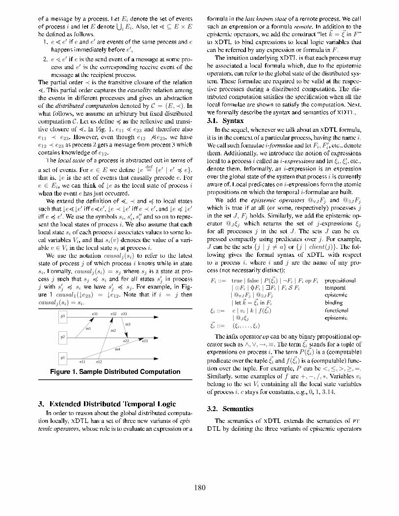
»ÚØß¾·Æ®Æ®Ø>ÀU¾ÞU×sØpÙOÅr»Âm¾·Æ®ÆTâ ¾>ÃEi

¿O¾nºj»Ã²¾*Ã Õ ¾QÆr¾>Ã[»Ú¾TÁO¾>ºOÃÉÆ»Ú;ÙOÅr»Âm¾·Æ1Æ

iØTºU¿3½¾>Ã

E¿O¾nºj»Ã¾ ⋃

i Ei

âë4½²Æ®»jáO½¾>Ã⊆ E × EÞj¾x¿U¾ Ü ºj¾n¿Ø·Æ)ÚZ»½½²»¼Æâõâ

e

e′Ö²Ú

eØTºj¿

e′ØTÅZ¾*¾TÁ¾nºOÃÉÆ»OÚ\Ã Õ ¾4Æ®ØTß¾ÙOÅr»Âm¾·Æ®ÆØTºj¿

eÕ ØTÙOÙj¾nºFÆ\Ößß¾n¿OÖ²Ø>þm½¤×ÞF¾nÚZ»Å¬¾e′á

#âe

e′ÖÚ

eÖÄÆÃ Õ ¾Æ¬¾>ºj¿Q¾TÁO¾>ºOÃ#»OÚdØ߾ƮÆrØnÀO¾*ØTÃ\Æ®»ß¾xÙOÅr»OÛ

Ân¾Æ®Æ4Ø>ºU¿e′ÖÄÆÃ Õ ¾Âm»ÅqŬ¾·ÆZÙF»ºj¿ÖºUÀÅZ¾mÂn¾nÖ¤Á¾¾TÁ¾nºOûOÚ Ã Õ ¾

ß¾·Æ1ÆrØ>ÀU¾Ø>ÃUÃ Õ ¾ ÅZ¾mÂ>ÖÙUÖ²¾>ºOÃUÙOÅr»Âm¾·Æ1ÆâÔ)Õ ¾4ÙFØÅZÃÖ²Øn½;»ÅZ¿U¾TÅ≺ÖÄÆ Ã Õ ¾ÃÅrØTºFƬÖÃÖ¤Á¾QÂn½²»UƬÝŬ¾Q»ÚÃ Õ ¾ÅZ¾m½Ø>ÃÖÄ»º

3â ÔÕ ÖÉÆÙFØÅZÃÖ²Øn½5»Å¬¿O¾>ÅÂmØÙjÃÝOÅZ¾ÆÃ Õ ¾4TJ¨®J¢ ¯QÅZ¾m½Ø>ÃÖÄ»ºØTß»ºUÀÃ Õ ¾ç¾TÁ¾nºOÃÉÆÖºð¿Ö²ÚÉÚh¾TŬ¾>ºOÃÙOÅr»Âm¾·Æ1Ƭ¾·ÆQØTºj¿`ÀOÖ¤Á¾ÆØ>ºðØTÞJƬäÅrØ>ÂnÃÖÄ»º»Ú)Ã Õ ¾ ± ²®¤©O¨ ± >¡¨¤j²¡O¿O¾nºj»Ã²¾n¿vÞj×

C = (E,≺)â÷hº

¼ Õ ØTÃdÚZ»½½»¼Æ áj¼¾ØmƮƬÝOß¾3ØTº9ØÅhÞUÖäÅrØÅZ×ÞÝUÃ Ü éO¾n¿ç¿ÖÉÆZÃÅhÖÞÝOò¾n¿Âm»ß3ÙjÝOÃÄØTÃÖ²»º

Câ ¾nÃ5ÝFÆ¿O¾ Ü ºU¾ñØmÆÃ Õ ¾*ÅZ¾J¾TéUÖ¤Á¾ØTºj¿3äÅrØTºJÆZÖÄÛ

ÃÖ¤ÁO¾Ân½²»UƬÝŬ¾»Ú3âJ÷qº`í#Ö²À#â+õ·áe11

e23Ø>ºU¿îÃ Õ ¾TŬ¾nÚZ»Å¬¾Ø>½ÄÆr»

e11 ≺ e23â 4»¼¾TÁ¾TÅZá+¾TÁO¾>ºåÃ Õ »ÝUÀ Õ

e12 6

e23áx¼¾ Õ ØÁ¾

e12 ≺ e23ØmÆ#ÙOÅr»Âm¾·Æ1Æ *ÀO¾nÃÄÆ;Ø+߾ƮÆrØnÀO¾+ÚÉÅr»ß'ÙOÅr»Ân¾Æ®Æ ¼ Õ Ö²Â Õ

Âm»ºUòØ>ÖºJÆ;¹OºF»¼½¾m¿OÀU¾ »Úe12â

ÔÕ ¾4¢¡jTJ¢F*»OÚ)Ø ÙUŬ»OÂn¾Æ®Æ)ÖÄÆHØTÞJÆZÃÅrØ>Â>ò¾n¿3»ÝUÃFÖº3ò¾TÅZßçÆ»OÚØƬ¾nÃd»OÚ¾TÁ¾nºOÃÉÆâí5»Å

e ∈ E¼¾4¿O¾ Ü ºU¾

↓edef= e′ | e′

eá

Ã Õ ØTÃ[ÖÉÆ1á↓eÖÉÆÃ Õ ¾Æ¬¾>Ã+»Ú¾TÁ¾nºOÃÉÆÃ Õ Ø>Ã)ÂmØTÝJÆrØn½½×sÙOŬ¾nÂn¾m¿O¾

eâUí5»Å

e ∈ Ei

á#¼¾3ÂmØ>ºsÃ Õ ÖºO¹L»OÚ↓eØmÆÃ Õ ¾3½²»ÂmØn½ÆZÃÄØTò¾»Ú+ÙOÅr»Âm¾·Æ1Æ

i¼ Õ ¾>ºÃ Õ ¾x¾TÁ¾nºOÃeÕ ØmÆ ¬ÝJÆZÃ#»ÂmÂ>ÝÅhŬ¾n¿#â

üY¾¾TéOò¾>ºj¿Ã Õ ¾3¿U¾ Ü ºUÖÃÖ²»º9»OÚQá≺ØTºj¿/ÃÄ»9½»OÂmØ>½Æ¬Ã²Ø>þÆ

ÆZÝUÂ Õ Ã Õ Ø>Ã↓e↓e′Ö²ÚÉÚ

e

e′á↓e ≺ ↓e′

ÖÚÉÚe ≺ e′

áTØTºj¿↓e

↓e′ÖÚÉÚ

e

e′âTüY¾xÝJƬ¾ Ã Õ ¾*ÆZ×Uß3ÞF»½ÄÆ

si

ás′iás′′iØTºj¿vÆr»Q»ºQò»ÅZ¾>ÙOŬ¾mÛ

Ƭ¾>ºUÃ#Ã Õ ¾*½»OÂmØn½\ÆZÃÄØTò¾·Æ»OÚ;ÙOÅr»Âm¾·Æ®Æiâmü`¾Øn½²Æ®»ØmÆ1ÆZÝOß¾pÃ Õ Ø>Ã5¾mØn Õ

½»OÂmØ>½jÆZÃÄØTò¾si

»OÚ5¾mØnÂ Õ ÙUŬ»OÂn¾Æ®ÆiØmÆ1Ær»ÂnÖ²Ø>þÆdÁØ>½ÝU¾Æ;ÃÄ»Ær»ß¾ ½»UÛÂmØ>½5ÁØÅZÖ²ØTÞj½¾·Æ

Vi

ájØ>ºU¿3Ã Õ ØTÃsi(v)

¿U¾>ºj»Ã¾ÆÃ Õ ¾ÁØ>½ÝU¾4»OÚØÁØTÅhÖÄÛØÞj½¾

v ∈ Vi

ÖºQÃ Õ ¾½²»Â·Ø>½JÆZÃÄØTò¾si

ØTÃjÙOÅr»Âm¾·Æ®Æiâ

üY¾îÝJƬ¾`Ã Õ ¾Lºj»Ã²Ø>ÃÖÄ»ºcausal j(si)

ÃÄ»(Ŭ¾nÚh¾TÅ3ò»CÃ Õ ¾î½²ØTò¾·Æ¬ÃÆZÃÄØTò¾v»OÚÙUŬ»OÂn¾Æ®Æ

j»ÚH¼ Õ Ö²Â Õ ÙOÅr»Âm¾·Æ®Æ

i¹OºF»¼Æ ¼ Õ Ö½¾QÖºLÆZÃÄØTò¾

si

âUí5»ÅhßØn½½×ácausal j(si) = sj

¼ Õ ¾>ÅZ¾sj

ÖÉÆpØ3ƬòØ>þØ>ÃdÙOÅr»OÛÂn¾·Æ1Æ

jÆZÝjÂ Õ Ã Õ ØTÃ

sj

si

ØTºU¿YÚZ»ÅØ>½½xÆZÃÄØTò¾·Æs′jÖºîÙUŬ»OÂn¾Æ®Æ

j¼*ÖÃ Õ

s′j

si

¼¾ Õ ØÁ¾s′j

sj

â;í5»Å¾>éjØTß3ÙF½¾á;Öº(í#ÖÀjÛÝŬ¾!õ

causal1(↓e23) = ↓e12⠻ò¾(Ã Õ ØTÃ4Ö²Ú

i = jÃ Õ ¾nº

causal j(si) = si

â

m1

p3

p2

p1

e31 e32 e33

e22 e23

e11 e12

m4

m3

m2

! "#%$&' )(*+ ' ! ,+ -

.Í0/21) FÏÑ FÑ YÓqUÓh+Ò FÑ43 %65Ð)j7 8Ð9dÓh÷hº»Å¬¿O¾>ÅdÃÄ»QŬ¾mØmÆ®»ºØÞJ»ÝOÃJÃ Õ ¾*ÀU½»ÞFØ>½F¿OÖÄƬäÅZÖ¤ÞÝUþm¿3Âm»ß3ÙjÝOÃÄØnÛ

ÃÖÄ»º½²»Â·Ø>½½¤×á ÿ ÔåÕ ØmÆ ØƬ¾nÃd»OÚ)Ã Õ Å¬¾n¾*ºU¾T¼ìÁØTÅhÖÄØTºUÃÄÆH»OÚq§TÇ>Q¤+¡ mhF¤¡FhTáT¼ Õ »jƬ¾Å¬»O½¾ÖÉÆ\ò»p¾TÁØ>½ÝjØ>þHØTº¾TéOÙOŬ¾·Æ1ÆZÖÄ»º»Å5Ø

Úh»ÅhßÝj½ØÖº4Ã Õ ¾x¢O OÊnj¡¥F »OÚ5Ø+Ŭ¾>߻þ+ÙUŬ»OÂn¾·Æ1Æâ ü`¾ÂmØ>½½ÆZÝjÂ Õ Ø>ºç¾TéOÙOŬ¾·Æ1ÆZÖÄ»ºç»ÅØQÚh»ÅhßÝj½ØQq>4¡Uâ÷hºsØn¿O¿OÖÃÖ²»ºÃÄ»Ã Õ ¾¾TÙjÖÄƬþnßÖ»ÙF¾TÅrØTÃĻŮÆ1á·¼¾4Øn¿O¿vÃ Õ ¾*Âm»ºFÆZÃÅZÝUÂ>Ã

let ~k = ~ξ in F

ò» ÿ Ô Ã²»sÞjÖºj¿L¾TéOÙOŬ¾·Æ®Æ¬Ö²»ºFÆxÃÄ».½»OÂmØn½½²»ÀÖ²ÂÁØTÅhÖÄØÞF½¾ÆÃ Õ ØTÃÂmØ>º4Þj¾ ÅZ¾mÚq¾>ÅqŬ¾n¿pÞj×vØ>º×¾TéOÙOŬ¾·Æ®Æ¬Ö²»ºQ»Å[ÚZ»ÅZßÝU½²ØHÖº

Fâ

Ô)Õ ¾HÖºOÃÝOÖÃÖÄ»º*ÝUºU¿O¾>ÅZ½×OÖºUÀ ÿ Ô ÖÄÆdÃ Õ ØTÃO¾·Ø>Â Õ ÙUŬ»OÂn¾Æ®Æ\ßØT×Þj¾Ø·Æ®Ær»OÂ>ÖÄØTò¾n¿Lؽ²»Â·Ø>½)ÚZ»ÅZßÝU½²Øv¼ Õ Ö²Â Õ á#¿OÝU¾vÃÄ»9Ã Õ ¾¾TÙjÖÄƬþnßÖ»ÙF¾TÅrØTÃĻŮÆ1á·ØTºpŬ¾nÚh¾TÅ#ÃÄ»pÃ Õ ¾ÀO½²»ÞFØn½OÆZÃÄØTò¾x»ÚFÃ Õ ¾¿OÖÄƬäÅZÖÞÝOò¾n¿4ÆZ×JÆrÛþnß.â Ô)Õ ¾Æ¬¾ÚZ»ÅZßÝU½²Ø>¾ØŬ¾pÅZ¾mæÝU֤Ŭ¾n¿vÃÄ»QÞj¾4ÁØn½¤Ö²¿ØTÃ#Ã Õ ¾ÅZ¾ÆhÙj¾mÂmÛÃÖÁ¾çÙOÅr»Ân¾Æ®Ær¾·Æv¿ÝOÅhÖºUÀ(Ø9¿ÖÉÆZÃÅZÖ¤ÞÝUþm¿Y·»ß3ÙjÝOÃÄØTÃÖ²»º5â Ô)Õ ¾9¿ÖÉÆrÛäÅZÖÞÝOò¾n¿Â·»ß3ÙjÝOÃÄØTÃÖ²»ºQÆrØTÃÖÉÆ Ü ¾Æ)Ã Õ ¾ÆhÙF¾nÂnÖ Ü Â·ØTÃÖ²»ºQ¼ Õ ¾>ºvØn½½jÃ Õ ¾½»OÂmØn½#Úh»ÅhßÝj½Øn¾ØŬ¾Æ Õ »¼*ºÃĻƮØTÃÖÄÆrÚA×Ã Õ ¾4·»ß3ÙjÝOÃÄØTÃÖ²»º5â ¾>éOÃAá¼¾xÚZ»ÅZßØ>½½¤×Q¿O¾·ÆrÂTÅZÖ¤ÞF¾Ã Õ ¾ÆZ×OºUòØ>éQØTºj¿vÆr¾>ßØTºUÃÖ²Â·Æ»Ú ÿ Ô â:';=<>;@?&A)BCEDF÷qºpÃ Õ ¾ Ƭ¾næOÝU¾m½ÄáT¼ Õ ¾>ºj¾TÁ¾TÅF¼¾+òØn½¤¹ØÞJ»ÝOÃØ>º ÿ Ô Úh»ÅhßÝj½Øá

ÖÃÖÉÆ\ÖºpÃ Õ ¾H·»ºOò¾TéUûOÚJØÙFØÅZÃÖÂnÝU½²ØÅjÙOÅr»Ân¾Æ®Æ á Õ ØÁOÖºjÀxÃ Õ ¾+ºFØTß¾iâü`¾+ÂmØ>½½ÆZÝjÂ Õ ÚZ»ÅZßÝU½²Ø>¾

iÇ ª ¡jZQ¨U¢§F)ØTºj¿ ½¾>Ã

Fi, F′i

á¾nÃÂOâ á ¿U¾>ºj»Ã¾Ã Õ ¾>ß.â·ë4¿O¿OÖÃÖ²»ºjØn½½×á¼¾*ÖºUäÅr»¿OÝUÂm¾Ã Õ ¾*ºF»ÃÖ²»º»Ú)¾TéOÙOŬ¾·Æ1ÆZÖÄ»ºFƽ»OÂmØn½Ã²»*ØÙOÅr»Âm¾·Æ1Æ

iÂmØ>½½¾n¿ØmÆ

iÇq¬«1h>®¤¡UdØ>ºU¿*½¾>Ã

ξi, ξ′i

á>¾>òÂâ á¿O¾nºj»Ã²¾Ã Õ ¾nß.âJ÷qºjÚh»ÅhßØn½½×á5ØTº

iÛq¾TéOÙOŬ¾·Æ®Æ¬Ö²»º.ÖÄÆQØTºY¾TéÙUÅZ¾Æ®Æ¬Ö²»º

»Á¾>ÅFÃ Õ ¾ÀU½»ÞFØn½OÆZÃÄØTò¾x»ÚJÃ Õ ¾xƬ×FƬþnß¸Ã Õ Ø>ÃÙOÅr»Âm¾·Æ®ÆiÖÄÆ[Â>ÝÅhŬ¾>ºOò½×

ØT¼ØŬ¾»Ú1â »OÂmØ>½·ÙUÅZ¾m¿Ö²ÂmØ>þÆ\»ºiÛq¾TéOÙOŬ¾·Æ®Æ¬Ö²»ºFÆ#Úh»Åhß'Ã Õ ¾ Ø>ò»ßÖÂ

ÙOÅr»ÙJ»UÆZÖÃÖ²»ºFÆd»ºv¼ Õ Ö²Â Õ Ã Õ ¾Ã²¾>ß3ÙF»Å¬Øn½iÛqÚh»ÅhßÝj½Øn¾HØTÅZ¾ ÞÝOÖ²½¤Ãhâ

ü`¾¸Øn¿O¿ñÃ Õ ¾ïh TQ!¡ mhF¤¡Fh@∀JFj

Ø>ºU¿@∃JFj¼ Õ Ö²Â Õ ÖÄÆ4äÅZÝU¾çÖ²Ú*Ø>à Ø>½½ »ÅÆr»ß¾á5Ŭ¾·ÆZÙj¾mÂ>ÃÖ¤Á¾n½× ÙOÅr»Âm¾·Æ®Ær¾·Æ jÖºÃ Õ ¾vƬ¾nÃ

JáFj

Õ »O½¿FÆâOòFÖßÖ²½ØTÅZ½×áO¼¾QØn¿O¿Ã Õ ¾Q¾TÙjÖÄƬþnßÖ»ÙFÛ¾TÅrØTÃÄ»Å

@Jξj

¼ Õ Ö²Â Õ Å¬¾>ÃÝÅZºFÆðÃ Õ ¾ìÆr¾>Ãî»OÚjÛq¾TéÙUÅZ¾Æ®Æ¬Ö²»ºFÆ

ξjÚh»ÅØ>½½*ÙOÅr»Âm¾·Æ®Ær¾·ÆjÖº!Ã Õ ¾CƬ¾nÃ

Jâ ÔÕ ¾CƬ¾nÃÄÆ

JÂmØTºåÞF¾ð¾TéjÛ

ÙOŬ¾·Æ1Ƭ¾n¿ð·»ß3ÙJØ>Â>ò½×YÝJÆZÖºUÀ`ÙOŬ¾n¿OÖ·ØTò¾·Æ3»ÁO¾TÅjâ[í5»ÅQ¾>éjØTß3ÙF½¾á

JÂmØTºÞj¾Ã Õ ¾3Ƭ¾>ÃÉÆ

j | j 6= aȁ

j | client(j)â Ô)Õ ¾4ÚZ»½²Û

½»¼*ÖºUÀìÀOÖ¤Á¾·Æ`Ã Õ ¾!ÚZ»ÅZßØ>½sÆZ×OºUòØ>é/»Ú ÿ Ô ¼*ÖÃ Õ Å¬¾·ÆZÙj¾mÂ>Ãò»,ØîÙOÅr»Ân¾Æ®Æ

iáH¼ Õ ¾TŬ¾

iØ>ºU¿

jØTÅZ¾`Ã Õ ¾LºFØTß¾Y»Ú3ØTº×gÙOÅr»OÛ

Ân¾Æ®Æ ºF»ÃOºj¾nÂm¾·Æ®Æ®ØÅZÖ½×Q¿OÖÄƬÃÖºUÂnà ãFi ::= true | false | P (~ξi) | ¬Fi | Fi op Fi GIHKJLGMJONQPRSP%JLTMU"V

| Fi | W · Fi | X Fi | Fi S Fi RSY#Z[G\J]HKU,V| @∀JFj | @∃JFj Y"G^P_NQRSY#Z`PSa| let ~k = ~ξi in Fi b PT^cdPT^e

ξi ::= c | vi | k | f(~ξi) f=g T^a,RP_JLT^U,V| @Jξj Y"G^P_NQRSY#Z`PSa

~ξi ::= (ξi, . . . , ξi)Ô)Õ ¾+Öº Ü é»ÙF¾TÅrØTÃÄ»ÅJ¡ ÂmØTºpÞF¾+Ø>º×xÞjÖºFØÅZ× ÙUŬ»ÙF»UƬÖÃÖÄ»ºjØn½·»ÙFÛ¾TÅrØTÃÄ»ÅÆZÝjÂ Õ ØmÆ

∧,∨,→,≡â Ô)Õ ¾xò¾TÅZß ~ξi

ÆZÃÄØTºU¿FÆÚh»Å[ØÃÝÙj½¾*»Ú¾TéÙUÅZ¾Æ®Æ¬Ö²»ºFÆ[»ºÙUŬ»OÂn¾·Æ1Æ

iâ Ô)Õ ¾xò¾TÅZß

P (~ξi)ÖÉÆØ Âm»ß3ÙjÝOÃÄØÞF½¾ ÙOŬ¾n¿OÖ·ØTò¾+»ÁO¾TÅJÃ Õ ¾+ÃÝOÙj½¾ ~ξi

ØTºj¿f(~ξi)

ÖÄÆ[Ø Âm»ß3ÙUÝUòØTÞj½¾ ÚqÝOºjÂmÛÃÖÄ»º.»Á¾>Å+Ã Õ ¾QÃÝÙj½¾âUí5»Å ¾TéFØTß3Ùj½¾áPÂmØ>ºÞF¾

<,≤, >,≥, =â

òFÖßÖ½²ØŬ½¤×áJÆr»ß¾3¾TéjØ>ß3Ùj½¾·Æ »OÚfØŬ¾

+,−, /, ∗âih+ØÅZÖ²ØTÞj½¾·Æ

viÞj¾m½»ºUÀÃÄ»Ã Õ ¾3Ƭ¾nÃVi

Âm»ºOÃÄØTÖºOÖºUÀØn½½;Ã Õ ¾v½»OÂmØn½dƬòØ>þ3ÁØÅZÖÄØÞj½¾·Æ»Ú5ÙOÅr»Âm¾·Æ®Æ

iâcÆZÃÄØT×JÆ)ÚZ»Å[Âm»ºFƬòØ>ºOÃÉÆ1ám¾â À#â á

0á1á3.14â

:';jk;@?l\mnD!BCoqp\rÔ)Õ ¾LƬ¾nßØTºUÃֲ·ÆQ»Ú ÿ Ô ¾TéOò¾>ºj¿jÆ4Ã Õ ¾9Ær¾>ßØTºUÃֲ·Æv»OÚýþÛ

ÿ Ô ÞU×s¿O¾ Ü ºOÖºUÀÃ Õ ¾QÃ Õ Å¬¾n¾vÁØÅZÖÄØTºOÃÉÆ »OÚH¾TÙUÖÉÆZò¾>ßֲ»ÙF¾TÅrØTÃĻŮÆ

180

C, si, [e] |= @∀JFj P f_f ∀j . (j ∈ J)→ C, sj , [e] |= Fj Y,HQY sj = causal j(si)C, si, [e] |= @∃JFj P f_f ∃j . (j ∈ J) ∧ C, sj , [e] |= Fj Y,HQY sj = causal j(si)C, si, [e] |= let (k, . . . , k′) = (ξi, . . . , ξ

′

i) in Fi P f_f C, si, [e, k 7→ (C, si, [e])[[ξi]], . . . , k′ 7→ (C, si, [e])[[ξ

′

i]]] |= Fi

(C, si, [e, k 7→ val ])[[k]] = val

(C, si, [e])[[@Jξj ]] = (C, sj , [e])[[ξj ]] | sj = causal j(si) ∧ j ∈ J

!$ !! -' ,! + ÿ ÔØTºU¿gÃ Õ ¾`ÞUÖºU¿ÖºUÀ,»Ùj¾>ŬØ>ò»Åhâ Ô)Õ ¾ðƬ¾nßØTºOÃֲ·ÆÖÄÆçÀOÖ¤Á¾>ºgÞU×,ÅZ¾·ÛÂ>ÝÅ®ÆZÖÁ¾n½×.¿O¾ Ü ºOÖºUÀ9Ã Õ ¾sÆ®ØTÃÖÄÆrÚqØnÂ>ÃÖ²»º.ÅZ¾m½Ø>ÃÖÄ»º

C, si, [e] |= Fi

á¼ Õ ¾TŬ¾

[e]ÖÉÆdØTº4¾nºÁOÖ¤År»ºUß¾>ºUÃmÂmØTÅqÅZ×OÖºUÀÃ Õ ¾ÞUÖºU¿OÖºjÀjÆ5Úh»Å5¿Ö²ÚÉÚq¾>ÅhÛ

¾>ºOÃU½»OÀÖ²Â+ÁØTÅhÖÄØÞF½¾Æ\¼ Õ Ö²Â Õ ÀO¾nÃÄÆ\ÖºOÃÅr»¿ÝjÂn¾m¿ Þj×Ã Õ ¾let

in

»Ùj¾>ŬØ>ò»Åhâ

(C, si, [e])[[ξi]]ÖÄÆÃ Õ ¾îÁØn½¤Ýj¾`»OÚ4Ã Õ ¾Y¾TéÙUÅZ¾Æ®ÆZÖÄ»º

ξiÖºçÃ Õ ¾3ƬòØ>þsi

ÝUºU¿U¾TÅÃ Õ ¾v¾>ºÁOÖ¤År»ºUß¾>ºOÃ[e]â Ô ØÞj½¾.õÚZ»ÅZßØ>½½¤×

ÀÖ¤Á¾Æ[Ã Õ ¾Æ¬¾nßØTºUÃֲ·Æ+»Ú;Ã Õ ¾ºU¾T¼à»Ùj¾>ŬØ>ò»ÅrÆ»Úÿ Ô â·í5»Å[Ã Õ ¾Æ¬¾>ßØ>ºOÃÖÂÆ+»Ú)»Ã Õ ¾>Å»Ùj¾>ŬØ>ò»ÅrÆ)Ã Õ ¾ÅZ¾·Ø>¿U¾TÅ®ÆØTÅZ¾Å¬¾nÚh¾TÅhÅZ¾m¿4ÃÄ»9ôúOörâü`¾ØmÆ1ÆZÝUß¾Ã Õ ØTÃ+¾TéÙUÅZ¾Æ®ÆZÖÄ»ºJÆ*ØŬ¾vÙOÅr»ÙF¾TŬ½¤×9Ã×Ùj¾m¿#â Ô ×ÙjÖ·Ø>½½¤×Ã Õ ¾·Æ¬¾xÃ×OÙj¾Æ[¼»Ýj½¿*ÞF¾ #ám¾>òÂâü`¾ Ø>½ÄÆr»Ø·Æ®ÆZÝUß¾HÃ Õ ØTÃ

si, s′i, s

′′i , . . .

ØTÅZ¾xƬòØ>þÆ[»ÚjÙUŬ»OÂn¾Æ®ÆiØ>ºU¿

sj , s′j , s

′′j , . . .

ØŬ¾pƬòØ>þƻOÚ#ÙUŬ»OÂn¾Æ®Æjâ

ÍÐ[ÏÓh1Ð)jÓhÏ 9Y 79dÐ)jÓq %Ô »ß»ºOÖÃĻŠÿ Ô ÚZ»ÅZßÝU½²Ø>¾*ÖºsØ¿O¾mÂn¾>ºUäÅrØ>½Ö²ên¾n¿3¼ØT×áU¼¾

ÆZ×OºUÃ Õ ¾·Æ¬Öêm¾ ± §1©O¨O ± 4¡OF¤¡FhØmÆvÚZ»½½»¼ÆTâ5í5»Å¾mØ>Â Õ ÙOÅr»OÛÂn¾·Æ1ÆÃ Õ ¾TŬ¾îÖÉÆ9ØðƬ¾TÙJØÅrØTò¾îß»ºOÖò»ÅZá+ÂmØn½½¾n¿­Øð¢¡jTJ¢4¡F¡j1á¼ Õ Ö²Â Õ Â Õ ¾mÂ>¹FÆJÃ Õ ¾½²»Â·Ø>½ ÿ Ô ÚZ»ÅZßÝU½²Ø>¾ØTºU¿ÂmØ>º*Ø>ÃÃÄØ>Â Õ Øn¿O¿ÖÄÛÃÖÄ»ºFØ>½JÖºUÚZ»ÅZßØTÃÖ²»ºQÃÄ»Ø>º×»ÝOòÀU»ÖºjÀvß¾·Æ®Æ®Ø>ÀU¾â Ô)Õ ÖÉÆ+ÖºUÚZ»ÅZßØnÛÃÖÄ»ºÂ·ØTºçÆZÝOÞJÆr¾næÝj¾>ºUý×vÞj¾4¾TéUäÅrØ>Ânþm¿QÞU×Ã Õ ¾4½²»Â·Ø>½Jß»ºOÖò»Å»ºÃ Õ ¾pÅZ¾mÂn¾>ÖÁÖºUÀÆZÖ²¿O¾¼*ÖÃ Õ »ÝUÃ5Â Õ ØTºUÀOÖºjÀÃ Õ ¾4ÝOºU¿U¾TŬ½¤×UÖºjÀvÆr¾>ßØTºFÛÃֲ·Æ*»OÚHÃ Õ ¾¿ÖÉÆZÃÅhÖÞÝOò¾n¿ÙOÅr»ÀŬØ>ß.â Ô)Õ ¾3½²»Â·Ø>½[ß»ºOÖò»Å »OÚ¾mØn ÕÙOÅr»Ân¾Æ®Æ

ißØ>ÖºUòØ>ÖºJÆ)Ø"!$#%'& )( !h +*\þ% ,¿UØ>òØmÛhƬäÅZÝUÂnÃÝOÅZ¾

KVi

áFƬò»ÅhÖºUÀÚZ»ÅH¾mØnÂ Õ ÙOÅr»Âm¾·Æ1ÆjÖºÃ Õ ¾QƬ×FƬþnß Ã Õ ¾ÆZÃÄØTÃÝFÆ »OÚ

Ø>½½[Ã Õ ¾ÆrØ>Úh¾>Ã×sÙF»O½¤Ö²ÂT×LÆZÝÞJÛAÚZ»ÅZßÝU½²Ø>¾vØTºj¿.ƬÝÞJÛA¾TéOÙOŬ¾·Æ1ÆZÖÄ»ºFÆHÅZ¾·ÛÚq¾>ÅqÅZÖºjÀpò»

jÃ Õ Ø>Ã

iÖÄÆØT¼ØŬ¾x»Ú1â Ô)Õ ¾¹OºF»¼½¾m¿OÀO¾HÁ¾mÂ>ÃÄ»Å

KVi

ÖÉÆØÙOÙF¾>ºj¿O¾n¿ ò»Ø>º×߾ƮƮØ>ÀO¾ Ær¾>ºOÃÞU×

iâ ü Õ ¾nºÙF¾TŬÚh»ÅhßÖºUÀØTº*ÖºFÛ

þ>ÅhºFØ>½Âm»ß3ÙUÝUòØ>ÃÖÄ»º4ÆZò¾TÙ5áTÃ Õ ¾xƬòØ>ÃÝJÆ[»Ú#Ã Õ ¾½»OÂmØ>½OÚh»ÅhßÝj½Øn¾+Ø>ºU¿¾TéÙUÅZ¾Æ®ÆZÖÄ»ºJÆFÖÉÆdØTÝUò»ßØTÃÖ·Ø>½½¤×pÝÙF¿UØTò¾n¿xÖº*Ã Õ ¾H½²»ÂmØn½¹OºF»¼½¾m¿OÀO¾Á¾nÂnò»Åhâ®ü Õ ¾>ºpÅZ¾mÂn¾nÖ¤ÁÖºUÀpØ+ß¾·Æ®Æ®Ø>ÀU¾+ÚAÅr»ß¸Ø>ºj»Ã Õ ¾>ÅUÙUŬ»OÂn¾Æ®Æ1áTÃ Õ ¾¹Oºj»¼½¾n¿UÀO¾QÁ¾nÂnò»ÅHÖÉÆÝÙF¿UØ>þm¿Ö²ÚHÃ Õ ¾vÅZ¾mÂn¾nÖ¤Á¾n¿çß¾·Æ1ÆrØnÀO¾3Âm»ºjÛòØ>ÖºJÆ+߻Ŭ¾*Ŭ¾nÂn¾nºOÃ\¹Oºj»¼½¾n¿UÀO¾ØÞJ»ÝUÃ\ØTº×ÙOÅr»Ân¾Æ®Æ+ÖºÃ Õ ¾3ÆZ×FÆ®Ûþnß.â Ô »¿j»Ã Õ ÖÉÆ1ájØ4Ær¾næOÝU¾>ºjÂn¾pºOÝUß3Þj¾>Ådºj¾n¾m¿jÆHØ>½ÄÆr»vÃÄ»vÞF¾*ßØTÖºjÛòØ>Öºj¾n¿ÚZ»Å\¾·Ø>Â Õ ÙUŬ»OÂn¾Æ®Æ;Öº4Ã Õ ¾¹Uºj»¼½¾n¿OÀU¾ÁO¾nÂ>ÃÄ»ÅZâ ºU½Ö¹U¾4ôúOöZáÃ Õ ¾¾>ºUäÅZÖ²¾·Æ »OÚ-!$#%'& )( !h +*\þ% ,`ØŬ¾ÆZ×Oß3ÞJ»½Ö¾TéÙUÅZ¾ÆrÛÆZÖÄ»ºFÆÖºFƬþ·Ø>¿.»ÚxÁØ>½ÝU¾·ÆTâ ÔÕ ÖÉÆÖÄÆ*¿OÝU¾vÃÄ»sÃ Õ ¾ÚqØ>ÂnÃ)Ã Õ ØTÃ+Ø>½½)Ã Õ ¾½»OÀÖ²ÂxÁØÅZÖÄØÞj½¾·Æ[Ŭ¾nÚh¾TÅhÅZ¾m¿ÖºØ>ºv¾TéOÙOŬ¾·Æ1ÆZÖÄ»ºv»ÅØÚZ»ÅZßÝU½²Ø>¾ ßØT׺j»Ã#Þj¾ØÁØ>Ö½²ØÞF½¾4Ø>Ã5Ã Õ ¾ÃÖß¾Q»Ú¾TÁØn½¤ÝFØTÃÖ²»º»Ú)Ã Õ ¾¾>éÙOŬ¾·Æ1ÆZÖÄ»º»Å\Ã Õ ¾pÚZ»ÅZßÝU½²Øâ Ô)Õ ¾>ÅZ¾mÚh»ÅZ¾á>Ã Õ ¾x¾TÁØ>½ÝjØ>ÃÖÄ»º»OÚ;ØxÚh»ÅhßÝj½Øx»Å)ØTº¾TéÙUÅZ¾Æ®ÆZÖÄ»ºpßØT×pÞF¾ÙJØÅZÃÖÄØ>½Éá>Âm»ºUòØ>ÖºUÖºjÀxÃ Õ ¾ÁØTÅhÖÄ»ÝJÆ#½²»ÀOÖÂÁØTÅhÖÄÛØÞj½¾·ÆTâ Ô)Õ ¾4½²»ÀOÖÂÁØTÅhÖÄØÞF½¾ÆÖºÃ Õ ¾·Æ¬¾Úh»ÅhßÝj½Øn¾*»Å¾TéOÙOŬ¾·Æ®Æ¬Ö²»ºFÆØŬ¾Å¬¾TÙF½ØnÂn¾m¿ Þj×ØnÂ>ÃÝjØn½ÁØ>½ÝU¾·Æ;»ºUÂn¾+Ã Õ ¾T×Þj¾mÂm»ß¾HØÁØ>Ö½²ØÞF½¾Oâ®ë¿O¾>ÃÄØTÖ²½¾n¿v¿ÖÉƬÂ>ÝJƮƬֲ»º»ÚdÃ Õ ¾Ø>½ÀU»ÅhÖÃ Õ ß/ÖÉÆÞj¾T×F»ºj¿4Ã Õ ¾Æ¬Â·»ÙF¾*»OÚ

Ã Õ ÖÄÆxÆ Õ »ÅhÃ#ÙFØÙF¾TÅZâ4»¼¾TÁ¾TÅZá·ÅZ¾·Ø>¿O¾>ÅrÆHØTÅZ¾ÅZ¾mÚq¾>ÅqŬ¾n¿vÃÄ»9ôúUá Oö)ÚZ»ÅÆr»ß¾»Ú\Ã Õ ¾pƬÖßÖ²½²ØÅdÖ¿U¾mØmÆTâ. Í/9Ð[Ï 7qÒÓhÐ[Ïü`¾9Þj¾m½¤Ö²¾TÁ¾sÃ Õ ØTÃÃ Õ ¾.½²»ÀOÖ ÿ Ô ÙOŬ¾·Ær¾>ºUþm¿îÖº(Ã Õ ÖÄÆÙJØnÛ

Ùj¾>ÅjÖÉÆ;Ø[ÙJ»¼¾TŬÚAÝj½>ÝOºj¿O¾>ÅZ½×OÖºUÀxÆZÙj¾nÂnÖ Ü ÂmØTÃÖÄ»ºÚZ»ÅZßØ>½ÖÉÆZß'ÚZ»ÅJ¿ÖÉÆrÛäÅZÖÞÝOò¾n¿4ÆZ×JÆZò¾>ßçÆâ>òjÙF¾nÂnÖ Ü Â·ØTÃÖ²»ºFÆ\¾TéOÙOŬ¾·Æ®Ær¾n¿ØmÆ ÿ Ô ÚZ»ÅZßÝjÛ½Øn¾HÂmØTºÞj¾+¾nÚAÚq¾mÂ>ÃÖ¤Á¾n½×xß»ºOÖò»ÅZ¾m¿Fá1¾TÁ¾nºxÖº*Ã Õ ¾+·»ºUþTéUûOÚF½ØTÅhÀO¾Æ¬Â·Ø>½¾ »Ùj¾nºp¿OÖÄƬäÅZÖÞÝOò¾n¿4ÆZ×JÆZò¾>ßçÆâ 4»¼¾TÁ¾>ÅZá1ÖÃÖÄÆ[¼*»ÅhÃ Õ ¼ Õ Ö½¾Ã²»ÖºÁ¾ÆZÃÖÀjØTò¾x»Ã Õ ¾>Å)¾TéOò¾>ºJÆZÖÄ»ºFÆ[Ã Õ ØTÃFÖºUÂTŬ¾mطƬ¾xÖÃÉÆ+¾TéÙUÅZ¾Æ®Æ¬Ö¤Á¾>ºj¾·Æ1Ƽ*ÖÃ Õ »ÝOÃJÆrØ>Â>ÅhÖ Ü ÂnÖºjÀ4Ã Õ ¾x¾mÚ Ü ÂnÖ¾nºUÂT×Q»OÚ5ß»ºOÖò»ÅhÖºUÀ5âY10ÏÐ2 7 FÑ 9 % FÏ1Ô)Õ ¾ Ü Å®ÆZÃ#Ã Õ Å¬¾n¾*ØTÝUÃ Õ »Å®Æ)ØTÅZ¾4ÆZÝOÙOÙJ»ÅZþm¿4ÖºQÙJØÅZÃjÞU×vÃ Õ ¾ÿëó43më÷53 Ô è Ô ëò+!63#Ŭ»OÀÅrØTßsáÂm»ºOÃŬØnÂ>Ãîí 87Uú97 jÛ:7;7UÛ UÛ57 1<újáÃ Õ ¾ÿxëó43·ë ÷>=è +ò Ô 3JÅr»ÀŬØ>ßsáÂm»ºUäÅrØ>Ânà í ú\õ OÛ57;õnÛ? Û õA@97;BFáYÃ Õ ¾ è ó ÅrØTºOà 79797dõFÛ:7 UÛõ>Û579B;õ jáîØTºU¿ Ã Õ ¾"C»ÃÄ»År»½²Ø ŬØ>ºOÃ4ó43\òDC ,ë Ô â Ô)Õ ¾C½²ØmƬÃ3Ø>ÝOÃ Õ »ÅÖÄÆYÆZÝOÙFÛÙF»Åhò¾n¿pÖº*ÙFØÅZÃÞj×Ã Õ ¾ ®»ÖºUà òFí1E ëòJë'ÀÅrØTºOà ?4? óxÛ57 \âF 1GF FÏ FH:IKJMLONQP R-SUTWVYXWTUV[Z]\^V`_9a'bdcef\:ghNjiWejk;NleATnmoOT]Pqp r4sYb sO\>p tuhXfPqpqeAT

v mb w xfLy)mb w xAZUz5| JdV g Z Y"~U~f^W ;U f )O ^UJ f4 _] V^NKY | PSY,Hia#PSY,T^a#YWO W;Ih U H JU g Z U,TIT edHQY#Y#PTOeR%J`cdP NKU#eLHQY Y )a TUTUX] N efPXfPqp NQPqpquKNK ]U IKU HUJ8 UEH=HqPSTOeIY,H 8 JdVSc b Y"Hqe 1-f U | Y,V g TOc U"T^c - Y,T g VSY b U NKY c H g TIRSPZY | Y,HqP¡>a U,RP%JdT £¢ TM¤ \eUu shshVfpTU¥UN$e^¦]Pi¨§5TfPsO\:TUX]yPpeATWXf _eAT©ªsO\sKTfuhs$eATnbªsO\5p tuhXfPqpeUTAR+«¨eAVfs _iWshuKgªp TW¥¬XUTWV­a ®]yNQP\¯XWuªPA§5TfPqsª\qk)\©s P X]PqpeUT v bf«l_9a'§Ww xO°fz5ª| JdV g Z Y WU J f9±; _8

H J² U,eIPT ³h U"V GMY"HqT '´)µ JONKY]N U,TOc µ¶· U"HQcdP `msKXWN¸eUTfp TW¥Xf®UefoUP]¹TfeAº shVU¥UsA1µM¢©»¨¼ HQYLN N 9IQU ~ H ~ J'µ Y#Y#T^UK½MN P[U"T^c ' U"ZU"T gQ¾ U,Z D Y]U]NKJdTIPT^e U b J g R Z YLN5N U#eIY GMU]N NQPT^e PT¿¡iTOPRSY4NQR%U,RSY Y#T | P HKJdTIZ Y,TOR_N ¢ T §5TfPsO\:TUX]yPpeATWXf_efqeUÀfoUpqoArÁeUTMa oWPeArXfPXAR ± XUTW¥foOXU¥UsKN¨XWTUV ¤ \eO¥8\©XWr-yr-p TW¥ v §Q_9a ± ¤ w xUxUz5 | JdV g Z Y I ~ J f9±9 _

H J¬- iY#T A · U"HQc U"T Uª e U ] U,TOc ÂO JON à g f ¡ a#PSY,TOR\cIY a#Y#TfRHKU"VPÄ#Y c ZJLTOPR%J]HqPSTOe J f N U f Y#RqÅ PST cdP_NQR HqP b g RSY cN:Å\NqR%Y,Z N Æ¢ T¤ \e]yu s sKV]p TU¥WNe^4SWÇfPi-§5TfPsO\:TUXfPpeATWXf+_eAT©ªsª\©sKTfuhs-eUTfe^OPºX]\s TW¥fpyTfshsO\>p TU¥ v §Q_ w xA°Wz v ea)kWk1shX]\:z>

181

Statistical Model Checking of Black-BoxProbabilistic Systems

Koushik Sen, Mahesh Viswanathan, Gul AghaDepartment of Computer Science,

University of Illinois at Urbana-Champaign.ksen,vmahesh,agha@uiuc.edu

Abstract. We propose a new statistical approach to analyzing stochas-tic systems against specifications given in a sublogic of continuousstochastic logic (CSL). Unlike past numerical and statistical analysismethods, we assume that the system under investigation is an unknown,deployed black-box that can be passively observed to obtain sample traces,but cannot be controlled. Given a set of executions (obtained by MonteCarlo simulation) and a property, our algorithm checks, based on statisti-cal hypothesis testing, whether the sample provides evidence to concludethe satisfaction or violation of a property, and computes a quantitativemeasure (p-value of the tests) of confidence in its answer; if the sampledoes not provide statistical evidence to conclude the satisfaction or vio-lation of the property, the algorithm may respond with a “don’t know”answer. We implemented our algorithm in a Java-based prototype toolcalled VeStA, and experimented with the tool using case studies ana-lyzed in [15]. Our empirical results show that our approach may, at leastin some cases, be faster than previous analysis methods.

1 Introduction

Stochastic models and temporal logics such as continuous stochastic logic(CSL) [1, 3] are widely used to model practical systems and analyze their per-formance and reliability. There are two primary approaches to analyzing thestochastic behavior of such systems: numerical and statistical. In the numericalapproach, the formal model of the system is model checked for correctness withrespect to the specification using symbolic and numerical methods. Model check-ers for different classes of stochastic processes and specification logics have beendeveloped [8, 14, 13, 4, 5, 2, 6]. Although the numerical approach is highly accu-rate, it suffers from being computation intensive. An alternate method, proposedby Younes and Simmons [16], is based on Monte Carlo simulation and sequen-tial hypothesis testing. Being statistical in nature, this approach is less accurateand only provides probabilistic guarantees of correctness. The approach doesnot assume knowledge of a specific formal model for the system being analyzed,and therefore can be potentially applied to analyzing complex dynamical sys-tems such as generalized semi-Markov processes (GSMPs), for which symbolicand numerical methods are impractical. However, the Younes and Simmons’ ap-proach assumes that the system is controllable (not black-box) and can be usedto generate sample executions from any state on need basis.

Both the numerical and the current statistical methods suffer from severalserious drawbacks when it comes to analyzing practical systems. First, modernday systems are large heterogeneous, and assembled by integrating equipment

182

and software from diverse vendors, making the construction of a formal model ofthe entire system often impossible and thus limiting the feasibility of numericaland symbolic methods. Second, for large network systems, meaningful experi-ments may involve dozens or even thousands of routers and hosts, which wouldmean that the system needs to be deployed before reasonable performance mea-sures can be obtained. However, once they are deployed, such systems cannot becontrolled to generate traces from any state, making it impossible to generateexecution samples on a need basis as is required by the Younes et. al’s statisticalapproach.

Despite the success of current analysis methods [10, 13, 12, 15, 8], there istherefore a need to develop methods to analyze stochastic processes that can beapplied to deployed, unknown “black-box” systems (systems from which tracescannot be generated from any state on need) 1. In this paper we address theseconcerns by proposing a new statistical approach to model checking. Like inYounes et. al’s approach, discrete event simulation methods are used to obtain aset of sample executions; however, unlike their method we assume no control overthe set of samples we obtain. We then test these samples using various statisticaltests determined by the property to be verified. Since we assume that the sam-ples are generated before testing, our algorithm relies on statistical hypothesistesting, rather than sequential hypothesis testing. Our inability to generate sam-ples of our choosing and at the time of our choosing ensures that our approachdiffers from the previous statistical approach in one significant way: unlike theprevious approach where the model checker’s answer can be guaranteed to becorrect within the required error bounds, we instead compute a quantitativemeasure of confidence (the p-value, in statistical testing terminology [11]) inthe model checker’s answer. Our algorithm computes the satisfaction of the de-sired formula by recursively determining the satisfaction of its subformulas (andthe confidence of such an answer) in the “states” present in the sample. Thispresents a technical challenge because our algorithm, being statistical in nature,may be uncertain about the satisfaction of some formulas based on the givensamples. The algorithm needs to compute useful answers (as far as possible)even in the presence of uncertain answers about the satisfaction of subformulas.We overcome this challenge by interpreting such “don’t know” answers in anadversarial fashion. Our algorithm, thus checks if the sample provides evidencefor the satisfaction or violation of a property and the confidence with which suchan assertion holds, or gives up and says “don’t know.” The algorithm that wepropose suffers from one drawback when compared with the previous statisticalapproach. Since we analyze a fixed sample, we will get useful answers only whenthere are sufficient samples for each “relevant state.” Therefore our method islikely to work well only when a finite set of samples is enough to provide sufficient

1 We assume that the samples generated from the system by discrete event simulationhave information about the “system state”. We, however, make no assumptionsabout the transition structure of the underlying system, nor do we assume knowledgeabout the transition probabilities; the system under investigation is black-box in thissense.

2

183

information about relevant states. Examples of systems we can successfully an-alyze are Continuous-time Markov Chains (CTMCs) or systems whose relevantstates are discrete, while we are unlikely to succeed for GSMPs in general.

A closely related approach to analyzing stochastic systems based on MonteCarlo simulation is by Herault et. al. [7], which can model-check discrete-timeMarkov chains against properties expressed in an expressively weak logic (“pos-itive LTL”).

We have implemented the whole procedure in Java as a prototype tool, calledVeStA (Verification based on Statistical Analysis).2 We have experimentedwith VeStA by applying it to some examples that have been previously analyzedin [15] and the results are encouraging. However, we suspect that VeStA wouldrequire a lot more space, because it stores the entire collection of samples it isanalyzing. Even though space was not a problem for the examples we tried, wesuspect that it may become an issue later.

The rest of the paper is organized as follows. Section 2 defines the class ofsystems we analyze and the logic we use. In Section 3, we present our algorithmbased on statistical hypothesis testing in detail. Details about VeStA and ourcase studies are presented in Section 4. In Section 5, we conclude and presentpossible directions for future research.

2 Preliminaries

2.1 Sample Execution Paths

The verification method presented here can be independent of the system modelas long as we can generate sample execution paths of the system; the modeland its definition are very similar to [16]. We will assume that the system beinganalyzed is some discrete event system that occupies some state s ∈ S, where Sis the set of states of the system. The states in S that can effect the satisfactionof a property of our interest are called the “relevant states.” Note that the num-ber of relevant states may be quite small compared to the whole state space ofthe system. For example, for a formula φ1 U≤tφ2 the states that can be reachedwithin time t are relevant. We assume that each relevant state can be uniquelyidentified and that information about a state’s identity is available in the exe-cutions. Since samples are generated before running our analysis algorithm, werequire that a Monte Carlo simulation is likely to generate a sample that hasenough “information” about the relevant states; if not our algorithm is likely tosay that it cannot infer anything about the satisfaction of the property.

We assume that there is a labeling function L that assigns to each state a setof atomic propositions (from among those appearing in the property of interest)that hold in that state; thus L : S → 2AP , where AP is a set of relevant atomicpropositions. The system remains in a state s until an event occurs, and thenproceeds instantaneously to a state s′. An execution path that appears in oursample is thus a sequence

π = s0t0→ s1

t1→ s2t2→ · · ·

2 Available from http://osl.cs.uiuc.edu/~ksen/vesta/

3

184

where s0 is the unique initial state of the system, si is the state of the systemafter the ith event and ti is the time spent in state si. If the kth state of thissequence is absorbing, then si = sk and ti = ∞ for all i ≥ k.

We denote the ith state in an execution π by π[i] = si and the time spentin the ith state by δ(π, i). The time at which the execution enters state π[i + 1]is given by τ(π, i + 1) =

∑j=ij=0 δ(π, j). The state of the execution at time t (if

the sum of sojourn times in all states in the path exceeds t), denoted by π(t), isthe smallest i such that t ≤ τ(π, i + 1). We let Path(s) be the set of executionsstarting at state s. We assume Path(s) is a measurable set (in an appropriateσ-field) and has an associated probability measure.

2.2 Continuous Stochastic Logic

Continuous stochastic logic (CSL) is introduced in [1] as a logic to express prob-abilistic properties of continuous time Markov chains (CTMCs). In this paperwe adopt a sublogic of CSL (excluding unbounded untils and stationary stateoperators) as in [16]. This logic excludes the steady-state probabilistic opera-tors and the unbounded until operators. We next present the syntax and thesemantics of the logic.CSL Syntax

φ ::= true | a ∈ AP | ¬φ | φ ∧ φ | P./p(ψ)

ψ ::= φ U≤tφ | Xφ

where AP is the set of atomic propositions, ./ ∈ <,≤, >,≥, p ∈ [0, 1], andt ∈ R≥0. Here φ represents a state formula and ψ represents a path formula. Thenotion that a state s (or a path π) satisfies a formula φ is denoted by s |= φ (orπ |= φ), and is defined inductively as follows:CSL Semantics

s |= true s |= a iff a ∈ AP(s)s |= ¬φ iff s 6|= φ s |= φ1 ∧ φ2 iff s |= φ1 and s |= φ2

s |= P./p(ψ) iff Probπ ∈ Path(s) | π |= ψ ./ pπ |= Xφ iff τ(π, 1) < ∞ and π[1] |= φ

π |= φ1 U≤tφ2 iff ∃x ∈ [0, t]. (π(x) |= φ2 and ∀y ∈ [0, x). π(y) |= φ1)

A formula P./p(ψ) is satisfied by a state s if Prob[path starting at s satisfiesψ] ./ p. To define probability that a path satisfies ψ we need to define a σ-algebraover the set of paths starting at s and a probability measure on the correspondingmeasurable space in a way similar to [5]. The path formula Xφ holds over a pathif φ holds at the second state on the path. The formula φ1 U≤tφ2 is true over apath π if φ2 holds in some state along π at a time x ∈ [0, t], and φ holds alongall prior states along π. This can also be recursively defined as follows:

Sat(siti→ πi+1, φ1 U≤tφ2)

= (t ≥ 0) ∧ (Sat(si, φ2) ∨ (Sat(si, φ1) ∧ Sat(πi+1, φ1 U≤t−tiφ2))) (1)

where Sat(s, φ) (or Sat(π, ψ)) are the propositions that s |= φ (or π |= ψ). Thisdefinition will be used later to describe the algorithm for verification of φ1U≤tφ2

formula.

4

185

3 Algorithm

In what follows we say that s |=A φ if and only if our algorithm (denoted by A)says that φ holds at state s. Since the algorithm is statistical, the decision madeby the algorithm provides evidence about the actual fact. In our approach, webound the strength of this evidence quantitatively by a number in [0, 1] whichgives the probability of making the decision given that the decision is actuallyincorrect. In statistics, this is called the p-value of the testing method. We denoteit by α3 and write s |= φ if the state s actually satisfies φ.

We assume that we are given a set of finite executions. The length of a finiteexecution path must be large enough so that all the bounded until formulas canbe evaluated on that path. Given a set of sample execution paths starting at theinitial state and a formula φ, the algorithm works recursively as follows:

verifyAtState(φ, s)if cache contains (φ, s) return cache(φ, s);

else if φ = true then (z, α) ← (1, 0.0);

else if φ = a ∈ AP then (z, α) ← verifyAtomic(a, s);

else if φ = ¬φ′ then (z, α) ← verifyNot(¬φ′, s);else if φ = φ1 ∧ φ2 then (z, α) ← verifyAnd(φ1 ∧ φ2, s);

else if φ = P./p(ψ) then (z, α) ← verifyProb(P./p(ψ), s);

store (s, φ) 7→ (z, α) in cache;

return (z, α);

where verifyAtState returns a pair having 0, 1, or undecided corresponding tothe cases s |=A φ, s 6|=A φ, or A cannot decide respectively, as the first compo-nent, and p-value for this decision as the second component. To verify a systemwe check if the given formula holds at the initial state. Once computed, we storethe decision of the algorithm for φ at state s in a cache to avoid recomputation.The result of our hypothesis testing can be shown to hold in presence of caching.This results in a significantly faster running time and a reduction in the sam-ple set size. In the remainder of this section we define the various proceduresverifyAtomic, verifyAnd, verifyNot, and verifyProb recursively.

The key idea of the algorithm is to statistically verify the probabilistic oper-ator. We present the corresponding procedure verifyProb below.3.1 Probabilistic OperatorWe use statistical hypothesis testing [11] to verify a probabilistic property φ =P./p(ψ) at a given state s. Without loss of generality we show our procedure forφ = P≥p(ψ). This is because, for the purpose of statistical analysis, P<p(ψ) isessentially the same as ¬P≥1−p(ψ) and < (or >) is in effect the same as ≤ (or≥). Let p′ be the probability that ψ holds over paths starting at s. We say thats |= P≥p(ψ) if and only if p′ ≥ p and s 6|= P≥p(ψ) if and only if p′ < p. Wewant to decide either s |= P≥p(ψ) or s 6|= P≥p(ψ). Accordingly we set up twoexperiments. In the first experiment, we use sample execution paths starting

3 This should not be confused with the Type I error which is also denoted by α

5

186

at s to test the null hypothesis H0 : p′ < p against the alternative hypothesisH1 : p′ ≥ p. In the second experiment, we test the null hypothesis H0 : p′ ≥ pagainst the alternative hypothesis H1 : p′ < p.4

Let the number of sample execution paths having a state s somewhere in thepath be n. We can treat the portion of all these paths starting at s (suffix) assamples from Path(s). Let X1, X2, . . . , Xn be a random sample having Bernoullidistribution with unknown parameter p′ ∈ [0, 1] i.e. for each i ∈ [1, n], Prob[Xi =1] = p′. Then the sum Y = X1 + X2 + . . . + Xn has binomial distribution withparameters n and p′. We say that xi, an observation of the random variableXi, is 1 if the ith sample execution path satisfies ψ and 0 otherwise. In thefirst experiment, we reject H0 : p′ < p and say s |=A P≥p(ψ) if

∑xi

n ≥ p andcalculate the p-value as α = Prob[s |=A φ | s 6|= φ] = Prob[Y ≥ ∑

xi | p′ < p].Note we do not know p′. Therefore, to calculate α we use p which is an upperbound for p′. If we are not able to reject H0 in the first experiment then we dothe second experiment. In the second experiment, we reject H0 : p′ ≥ p and says 6|=A P≥p(ψ) if

∑xi

n < p and calculate the p-value as α = Prob[s 6|=A φ | s |=φ] = Prob[Y <

∑xi | p′ ≥ p]. Thus, a smaller α represents a greater confidence

in the decision of the algorithm A.

3.2 Nested Probabilistic Operators

The above procedure for hypothesis testing works if the truth value of ψ overan execution path determined by the algorithm is the same as the actual truthvalue. However, in the presence of nested probabilistic operators in ψ, A cannotdetermine the satisfaction of ψ over a sample path exactly. Therefore, in thissituation we need to modify the hypothesis test so that we can use the inexacttruth values of ψ over the sample paths.

Let the random variable X be 1 if a sample execution path π actually satisfiesψ in the system and 0 otherwise. Let the random variable Z be 1 for a sampleexecution path π if π |=A ψ and 0 otherwise. In our procedure we cannot getsamples from the random variable X; instead our samples come from the ran-dom variable Z. Let X and Z have Bernoulli distributions with parameters p′

and p′′ respectively. Let Z1, Z2, . . . , Zn be a random sample from the Bernoullidistribution with unknown parameter p′′ ∈ [0, 1]. We say that zi, an observationof the random variable Zi, is 1 if the algorithm says that the ith sample executionpath satisfies ψ and 0 otherwise.

For the formula φ = P≥p(ψ) we calculate regions of indifference, denoted bythe fractions δ1 and δ2, based on the algorithm’s decision for the satisfactionof ψ over the different sample paths. Depending on the values of δ1 and δ2 weset up the two experiments. In the first experiment, we test the null hypothesisH0 : p′′ ≤ p + δ1 against the alternative hypothesis H1 : p′′ > p + δ1. If we get∑

zi

n > p + δ1 we reject H0 and say s |=A P≥p(ψ) with p-value α = Prob[s |=Aφ | s 6|= φ] = Prob[

∑Zi >

∑zi | p′′ ≤ p + δ1]. If we fail to reject H0 we

4 While handling nested probabilistic operators, these experiments will no longer besymmetric. Moreover, setting up these two experiments is an alternate way of gettingat a conservative estimate of what Type II error (β value) may be.

6

187

go for the second experiment, in which the null hypothesis H0 : p′′ ≥ p − δ2

against the alternative hypothesis H1 : p′′ < p − δ2. We reject H0 and say thats 6|=A P≥p(ψ) if

∑zi

n < p − δ2 and calculate the p-value as α = Prob[s 6|=A φ |s |= φ] = Prob[

∑Zi <

∑zi | p′′ ≥ p − δ2]. Otherwise, we say the algorithm

cannot decide.We now show how to calculate δ1 and δ2. Using the samples from Z we can

estimate p′′. However, we need an estimation for p′ in order to decide whetherφ = P≥p(ψ) holds in state s or not. To get an estimate for p′ we note that therandom variables X and Z are related as follows:

Prob[Z = 0 | X = 1] ≤ α′ Prob[Z = 1 | X = 0] ≤ α′

where α′ is the p-value calculated while verifying the formula ψ. By elementaryprobability theory, we have

Prob[Z = 1] = Prob[Z = 1 | X = 0]Prob[X = 0] + Prob[Z = 1 | X = 1]Prob[X = 1]

Therefore, we can approximate p′′ = Prob[Z = 1] as follows:

Prob[Z = 1] ≤ α′(1− p′) + 1.p′ = p′ + (1− p′)α′

Prob[Z = 1] ≥ Prob[Z = 1 | X = 1]Prob[X = 1] ≥ (1− α′)p′ = p′ − α′p′

This gives the following range in which p′′ lies:

p′ − α′p′ ≤ p′′ ≤ p′ + (1− p′)α′

Hence, Prob[∑

Zi >∑

zi | p′ ≤ p] ≤ Prob[∑

Zi >∑

zi | p′ = p] ≤Prob[

∑Zi >

∑zi | p′′ = p − α′p] which gives δ2 = α′p. Similarly, we get

δ1 = (1− p)α′.Note that the p-value obtained while verifying ψ over different sample paths

are different. We take the worst or the maximum of all such p-values as α′.Moreover, since A can say true, false, or cannot decide, note that the A may nothave a definite true or false answer along certain sample paths. For such pathsthe algorithm will assume the worst possible answer in the two experiments. Forthe first experiment, where we check whether

∑zi

n > p+ δ1, we take the answersfor the sample paths for which A cannot decide as false and the p-value as 0.For the second experiment we consider the answer for the undecided paths tobe true and the p-value as 0. This allows us to obtain useful answers even whenthe sample does not have enough statistical evidence for the satisfaction of asubformula.

Thus we can define the procedure verifyProb(P≥p(ψ), s) as follows:

verifyProb(P≥p(ψ), s)zsummin ← 0; zsummax ← 0; α′ ← 0.0; n ← 0;

for each sample path π starting at s(z, α′′) ← verifyPath(ψ, π);

if z =undecided then zsummin ← zsummin + 1; zsummax ← zsummax + 0;else zsummin ← zsummin + z; zsummax ← zsummax + z;α′ ← max (α′, α′′); n ← n + 1;

7

188

if zsummax/n > p + (1− p)α′ then

return (1,Prob[∑

Zi > zsummax | p′′ = p + (1− p)α′]);else if zsummin/n < p− pα′ then

return (0,Prob[∑

Zi < zsummin | p′′ = p− pα′]);else return (undecided , 0.0);

One can calculate Prob[

∑Zi > zsummax | p′′ = p+(1−p)α′] (or Prob[

∑Zi >

zsummin | p′′ = p − pα′]) by noting that∑

Zi has binomial distribution withparameters p + (1− p)α′ (or p− pα′) and n.

3.3 Negation

For the verification of a formula ¬φ at a state s, we recursively verify φ at states. If s |=A φ with p-value α we say that s 6|=A ¬φ with p-value Prob[s 6|=A ¬φ |s |= ¬φ] = Prob[s |=A φ | s 6|= φ] = α. Similarly, if s 6|=A φ with p-value α thens |=A ¬φ with p-value α. Otherwise, if A cannot answer the satisfaction of φ ats, we say that A cannot answer the satisfaction of ¬φ at s. Thus we can defineverifyNot as follows:

verifyNot(¬φ′, s)(z, α) ← verifyAtState(φ′, s);if z =undecided then return (undecided , 0.0); else return (1− z, α);

3.4 Conjunction

To verify a formula φ = φ1 ∧ φ2 at a state s, we verify φ1 and φ2 at the state sseparately. Depending on the outcome of the verification of φ1 and φ2, A decidesfor φ as follows:

1. If s |=A φ1 and s |=A φ2 with p-values α1 and α2 respectively, then s |=A φ.The p-value for this decision is Prob[s |=A φ1 ∧ φ2 | s 6|= φ1 ∧ φ2]. Note thats 6|= φ1 ∧ φ2 holds in three cases, namely 1) s 6|= φ1 and s |= φ2, 2) s |= φ1

and s 6|= φ2, and 3) s 6|= φ1 and s 6|= φ2. Thus, the p-value for the decisionof s |=A φ can be taken as the maximum of the p-values in the above threecases which is max (α1, α2).

2. If s 6|=A φ1 (or s 6|=A φ2) and either s |=A φ2 or A cannot decide φ2 at s (oreither s |=A φ1 or A cannot decide φ1 at s), then s 6|=A φ and the p-value isProb[s 6|=A φ1 ∧ φ2 | s |= φ1 and s |= φ2] = α1 + α2 (or α2 + α1).

3. If s 6|=A φ1 and s 6|=A φ2 then s 6|=A φ1 ∧ φ2. The p-value for this decision isProb[s 6|=A φ1 ∧ φ2 | s |= φ1 and s |= φ2] ≤ α1 + α2.

4. Otherwise, A cannot decide φ.

Thus we can define the procedure verifyAnd as follows:

verifyAnd(φ1 ∧ φ2, s)(z1, α1) ← verifyAtState(φ1, s); (z2, α2) ← verifyAtState(φ2, s);

8

189

if z1 = 1 and z2 = 1 then return (1,max (α1, α2));

else if z1 = 0 and z2 6= 0 then return (0, α1 + α2);

else if z1 6= 0 and z2 = 0 then return (0, α1 + α2);

else if z1 = 0 and z2 = 0 then return (0, α1 + α2);

else return (undecided , 0.0);

3.5 Atomic Proposition

In this simplest case, given φ = a and a state s, A checks if s |=A a or notby checking if a ∈ AP(s) or not. If a ∈ AP(s) then s |=A φ with p-value 0.Otherwise, s 6|=A φ with p-value 0.

verifyAtomic(a, s)if a ∈ AP(s) then return (1, 0.0); else return (0, 0.0);

3.6 Next

To verify a path formula ψ = Xφ over a path π, A verifies φ at the stateπ[1]. If π[1] |=A φ with p-value α then π |=A ψ with p-value α. Otherwise, ifπ[1] 6|=A φ with p-value α then π 6|=A ψ with the same p-value. Thus we candefine verifyPath for Xφ as follows:

verifyPath(Xφ, π)return verifyAtState(φ, π[1]);

3.7 Until

Let ψ = φ1 U≤tφ2 be an until formula that we want to verify over the path π.We can recursively evaluate the truth value of the formula over the path π byfollowing the recursive definition given by Equation 1. Given the truth value andthe p-value for the formula φ1U≤t′−tiφ2 over the suffix πi+1, we can calculate thetruth value of φ1 U≤t′φ2 over the path πi by applying the decision procedure forconjunction and negation. Observe that the recursive formulation in Equation 1can be unrolled to obtain an equation purely in terms of conjuction and negation(and without any until formulas); it is this “unrolled” version that is used in theimplementation for efficiency reasons.

4 Implementation and Performance

We have implemented the above algorithm as part of a prototype Java toolcalled VeStA. We successfully used the tool to verify several programs havinga CTMC model.5 The performance of the verification procedure depends on thenumber of samples required to reach a decision with sufficiently small p-value. Toget a smaller p-value the number of samples needs to be increased. We need a lotof samples only when the actual probability of a path from a state s satisfying a5 We selected systems with CTMC model so that we can compare our results with

that of existing tools.

9

190

formula ψ is very close to the threshold p in a formula P./p(ψ) whose satisfactionwe are checking at s.

To evaluate the performance and effectiveness of our implementation we dida few case studies. We mostly took the stochastic systems used for case studiesin [15]. The experiments were done on a 1.2 GHz Mobile Pentium III laptoprunning Windows 2000 with 512 MB memory.6 We did not take into account thetime required for generating samples: we assumed that such samples come froma running system. However, this time, as observed in some of our experiments,is considerably less than the actual time needed for the analysis. We generatedsamples of length sufficient to evaluate all the time-bounded until formulas. Inall of our case studies we checked the satisfaction of a given formula at the ini-tial state. We give a brief description of our case studies below followed by ourresults and conclusions. The details for the case studies can be obtained fromhttp://osl.cs.uiuc.edu/~ksen/vesta/.

Grid World: We choose this case study to illustrate the performance of ourtool in the presence of nested probabilistic operators. It consists of an n × ngrid with a robot located at the bottom-left corner and a janitor located at thetop-right corner of the grid. The robot first moves along the bottom edge of acell square and then along the right edge. The time taken by the robot to movefrom one square to another is exponentially distributed. The janitor also movesrandomly over the grid. However, either the robot or the janitor cannot move toa square that is already occupied by the other. The robot also randomly sendsa signal to the base station. The underlying model for this example is a CTMC.The aim of the robot is to reach the top-right corner in time T1 units with prob-ability at least 0.9, while maintaining a minimum 0.5 probability of communica-tion with the base station with periodicity less than T2 units of time. This can bespecified using the CSL formula P≥0.9(P≥0.5(trueU≤T2communicate)U≤T1goal).

10-2

10-1

100

101

102

102 103 104 105 106 107

time

in s

ec

no. of states

101

102

103

104

102 103 104 105 106 107

no. o

f sam

ples

no. of states

Fig. 1. Grid world: verification time and number of samples versus number of states.

We verified the CSL property for Grid World with n ∈ [1, 100]. The propertyholds only for n ∈ [1, 13]. The state space of the program is Θ(n3). In Fig.1 we6 [15] used a 500 MHz Pentium III. However, our performance gain due to the use of

faster processor is more than offset by the use of Java instead of C.

10

191

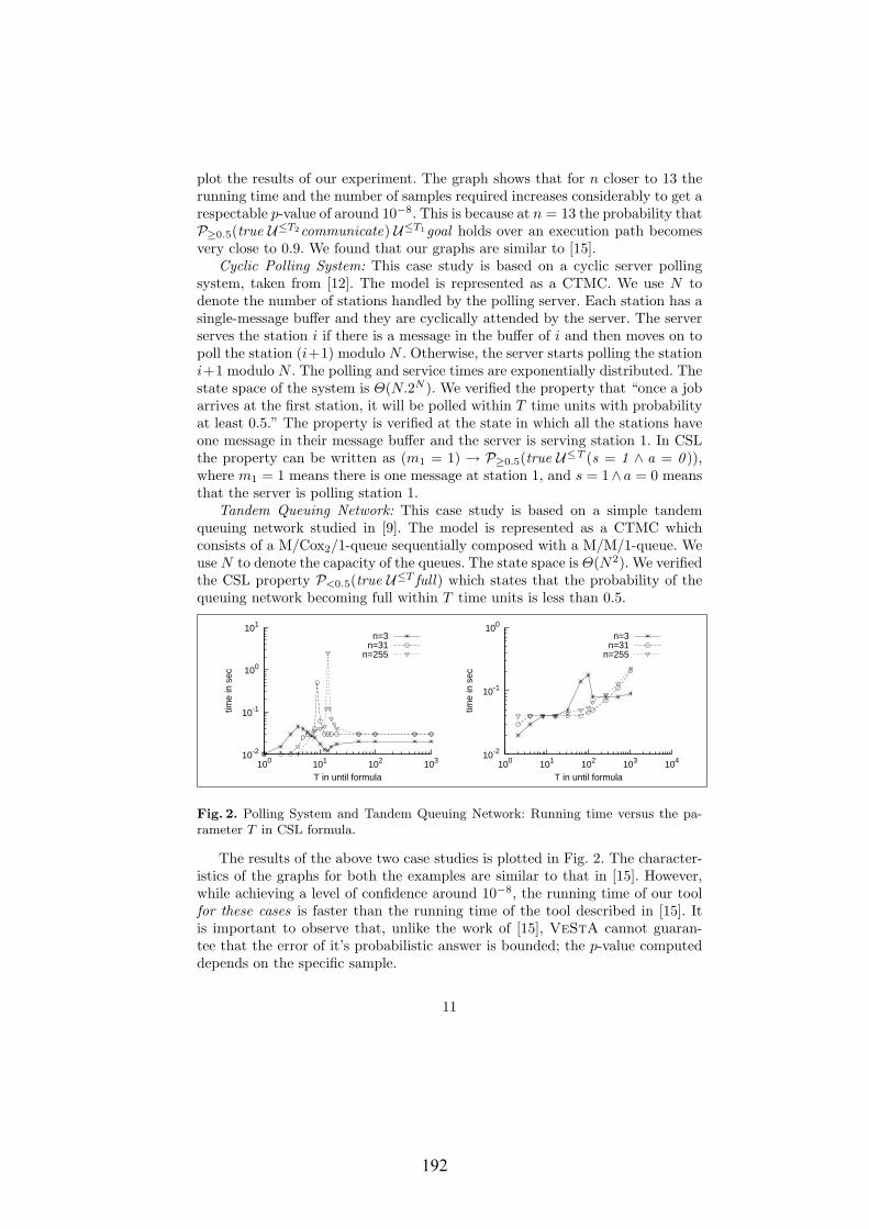
plot the results of our experiment. The graph shows that for n closer to 13 therunning time and the number of samples required increases considerably to get arespectable p-value of around 10−8. This is because at n = 13 the probability thatP≥0.5(true U≤T2communicate) U≤T1goal holds over an execution path becomesvery close to 0.9. We found that our graphs are similar to [15].

Cyclic Polling System: This case study is based on a cyclic server pollingsystem, taken from [12]. The model is represented as a CTMC. We use N todenote the number of stations handled by the polling server. Each station has asingle-message buffer and they are cyclically attended by the server. The serverserves the station i if there is a message in the buffer of i and then moves on topoll the station (i+1) modulo N . Otherwise, the server starts polling the stationi+1 modulo N . The polling and service times are exponentially distributed. Thestate space of the system is Θ(N.2N ). We verified the property that “once a jobarrives at the first station, it will be polled within T time units with probabilityat least 0.5.” The property is verified at the state in which all the stations haveone message in their message buffer and the server is serving station 1. In CSLthe property can be written as (m1 = 1) → P≥0.5(true U≤T (s = 1 ∧ a = 0 )),where m1 = 1 means there is one message at station 1, and s = 1∧ a = 0 meansthat the server is polling station 1.

Tandem Queuing Network: This case study is based on a simple tandemqueuing network studied in [9]. The model is represented as a CTMC whichconsists of a M/Cox2/1-queue sequentially composed with a M/M/1-queue. Weuse N to denote the capacity of the queues. The state space is Θ(N2). We verifiedthe CSL property P<0.5(true U≤T full) which states that the probability of thequeuing network becoming full within T time units is less than 0.5.

10-2

10-1

100

101

100 101 102 103

time

in s

ec

T in until formula

n=3n=31

n=255

10-2

10-1

100

100 101 102 103 104

time

in s

ec

T in until formula

n=3n=31

n=255

Fig. 2. Polling System and Tandem Queuing Network: Running time versus the pa-rameter T in CSL formula.

The results of the above two case studies is plotted in Fig. 2. The character-istics of the graphs for both the examples are similar to that in [15]. However,while achieving a level of confidence around 10−8, the running time of our toolfor these cases is faster than the running time of the tool described in [15]. Itis important to observe that, unlike the work of [15], VeStA cannot guaran-tee that the error of it’s probabilistic answer is bounded; the p-value computeddepends on the specific sample.

11

192

We could not compare the number of samples for these case studies as theyare not available from [15]; theoretically sequential hypothesis testing shouldrequire a smaller sample size than simple hypothesis testing to achieve the samelevel of confidence. While in our case studies we never faced a memory problem,we suspect that this may be a problem in very big case studies. We observedthat, although the state space of a system may be large, the number of statesthat appeared in the samples may be considerably smaller. This gives us hopethat our approach may work as well for very large-scale systems.

5 Conclusion and Future Work

We have presented a new statistical approach to verifying stochastic systemsbased on Monte Carlo simulation and statistical hypothesis testing. The maindifference between our approach and previous statistical approaches is that weassume that the system under investigation is not under our control. This meansthat our algorithm computes on a fixed set of executions and cannot obtain sam-ples as needed. As a consequence, the algorithm needs to check for the satisfac-tion of a property and compute the p-value of its tests. Since the sample may notprovide sufficient statistical evidence to conclude the satisfaction or violation of aproperty, one technical challenge is to provide useful answers despite insufficientstatistical evidence for the satisfaction of subformulas. We implemented our ap-proach in Java and our experimental case studies have demonstrated that therunning time of our tool is faster than previous methods for analyzing stochasticsystems in at least some cases; this suggests that our method may be a feasiblealternative.

Another important challenge is the amount of memory needed. Since westore all the sample executions, our method is memory intensive, and thoughwe did not suffer from memory problems on the examples studied here, we sus-pect that it will be an issue when analyzing larger case studies. Hence, thereis a need to design efficient data structures and methods to store and computewith a large set of sample executions. We suspect statistical hypothesis testingapproaches (as opposed to sequential hypothesis testing approaches) might beextendible to check liveness for certain types of systems, possibly by extract-ing some additional information about the traces. Note that liveness propertiesare particularly complicated by the fact that the operators may be nested. Weare currently exploring that direction. Finally, it would be interesting to applystatistical methods to analyze properties described in probabilistic logics otherthan CSL.

Acknowledgments

The work is supported in part by the DARPA IPTO TASK Award F30602-00-2-0586,the DARPA IXO NEST Award F33615-01-C-1907, the DARPA/AFOSR MURI AwardF49620-02-1-0325, the ONR Grant N00014-02-1-0715, and the Motorola Grant MO-TOROLA RPS #23 ANT. We would also like to acknowledge the contribution of JoseMeseguer to this research. Our work has benefitted considerably from stimulating dis-cussions with him and from our many years of collaboration on probabilistic rewritingtheories. We would like to thank Reza Ziaie for reviewing a previous version of thispaper and giving us valuable feedback.

12

193

References

1. A. Aziz, K. Sanwal, V. Singhal, and R. K. Brayton. Verifying continuous-timeMarkov chains. In 8th International Conference on Computer Aided Verification(CAV’96), volume 1102, pages 269–276. Springer, 1996.

2. R. Alur, C. Courcoubetis, and D. Dill. Model-checking for probabilistic real-timesystems (extended abstract). In Proceedings of the 18th International Colloquiumon Automata, Languages and Programming (ICALP’91), volume 510 of LNCS,pages 115–126. Springer, 1991.

3. A. Aziz, K. Sanwal, V. Singhal, and R. Brayton. Model-checking continuous-timeMarkov chains. ACM Transactions on Computational Logic, 1(1):162–170, 2000.

4. C. Baier, E. M. Clarke, V. Hartonas-Garmhausen, M. Z. Kwiatkowska, andM. Ryan. Symbolic model checking for probabilistic processes. In Proceedingsof the 24th International Colloquium on Automata, Languages and Programming(ICALP’97), volume 1256 of LNCS, pages 430–440. Springer, 1997.

5. C. Baier, J. P. Katoen, and H. Hermanns. Approximate symbolic model checkingof continuous-time markov chains. In International Conference on ConcurrencyTheory, volume 1664 of LNCS, pages 146–161. Springer, August 1999.

6. A. Bianco and L. de Alfaro. Model checking of probabilistic and nondeterministicsystems. In Proceedings of 15th Conference on the Foundations of Software Tech-nology and Theoretical Computer Science (FSTTCS’95), volume 1026 of LNCS.

7. T. Herault, R. Lassaigne, F. Magniette, and S. Peyronnet. Approximate Proba-bilistic Model Checking. In Proceedings of Fifth International Conference on Ver-ification, Model Checking and Abstract Interpretation (VMCAI’04), volume 2937of LNCS, pages 73–84. Springer, 2004.

8. H. Hermanns, J. P. Katoen, J. Meyer-Kayser, and M. Siegle. A Markov chainmodel checker. In Tools and Algorithms for Construction and Analysis of Systems(TACAS’00), pages 347–362, 2000.

9. H. Hermanns, J. Meyer-Kayser, and M. Siegle. Multi-terminal binary decisiondiagrams to represent and analyse continuous-time markov chains. In Proceed-ings of 3rd International Workshop on the Numerical Solution of Markov Chains(NSMC’99), 1999.

10. J. Hillston. A Compositional Approach to Performance Modelling. CambridgeUniversity Press, 1996.

11. R. V. Hogg and A. T. Craig. Introduction to Mathematical Statistics. Macmillan,New York, NY, USA, fourth edition, 1978.

12. O. C. Ibe and K. S. Trivedi. Stochastic petri net models of polling systems. IEEEJournal on Selected Areas in Communications, 8(9):1649–1657, 1990.

13. M. Z. Kwiatkowska, G. Norman, and D. Parker. Prism: Probabilistic symbolicmodel checker, 2002.

14. M. Z. Kwiatkowska, G. Norman, R. Segala, and J. Sproston. Verifying quantitativeproperties of continuous probabilistic timed automata. In International Conferenceon Concurrency Theory (CONCUR’00), volume 1877 of LNCS, pages 123–137.Springer, 2000.

15. H. L. S. Younes, M. Kwiatkowska, G. Norman, and D. Parker. Numerical vs.statistical probabilistic model checking: An empirical study. In 10th InternationalConference on Tools and Algorithms for the Construction and Analysis of Systems(TACAS’04). Springer, 2004.

16. H. L. S. Younes and R. G. Simmons. Probabilistic verification of discrete eventsystems using acceptance sampling. In 14th International Conference on ComputerAided Verification (CAV’02), volume 2404 of LNCS, pages 223–235. Springer, 2002.

13

194

Maximal Clique Based Distributed Group Formation for Autonomous

Agent Coalitions

Predrag Tosic∗, Gul AghaOpen Systems Laboratory, Department of Computer Science

University of Illinois at Urbana-Champaign, USAp-tosic, agha@cs.uiuc.edu

Abstract

We present herein a fully distributed algorithmfor group or coalition formation among au-tonomous agents. The algorithm is based ona distributed computation of maximal cliques(of up to pre-specified size) in the underlyinggraph that captures the interconnection topol-ogy of the agents. Hence, given the currentconfiguration of the agents, the groups that areformed are characterized by a high degree ofconnectivity, and therefore high fault tolerancewith respect to node and link failures. We alsobriefly discuss how our basic algorithm can beadapted in various ways so that the formedgroups satisfy the requirements (“goodness” cri-teria) other than mere strong inter-group com-munication connectivity. We envision variousvariants of our basic algorithm to prove them-selves useful subroutines in many multi-agentsystem and ad hoc network applications wherethe agents may repeatedly need to form tempo-rary groups or coalitions in an efficient, fullydistributed and online manner.

Keywords: distributed algorithms, dis-tributed group formation, multi-agent systems,autonomous agents, agent coalitions

1 Introduction and Motivation

Multi-agent systems (MAS) are characterized, amongother properties, by (i) considerable degree of au-tonomy of individual computing entities or processes(agents) and, at the same time, the fact that (ii) eachagent has a local, that is, in general, incomplete andimperfect “picture of the world”. Since in MAS there

is either no central control, or at best only a limitedcentral control, and the individual agents have to boththink and act locally, genuinely distributed algorithmsare needed for the agents to effectively coordinate withone another. MAS pose a number of challenges to a dis-tributed algorithm designer; most of these challengesare related to various aspects of the agent coordina-tion problem [1, 18]. In order to be able to effectivelycoordinate, agents need to be able to reach consen-sus (or agreement) on various matters of common in-terest. Two particularly prominent and frequently en-countered consensus problems are those of leader elec-tion (e.g., [6, 15]) and group formation.

Group formation is an important issue in dis-tributed systems in general, and MAS in particular.Given a collection of computational and communicat-ing agents, the goal in distributed group formation isthat these agents, based on their local knowledge only,decide how to effectively split up into several groups,so that each agent knows what group(s) it belongs to.

There are several critical issues that a MAS designerneeds to address in the context of (distributed) groupformation. First, what is the right notion of a group in agiven setting? That is, how is the quality of a particulargroup configuration measured, so that one can say thatone grouping of agents into coalitions is better for thatagent and/or for the whole system than another? Sec-ond, a distributed group formation mechanism - thatis, a distributed algorithm that enables agents to effec-tively form groups or coalitions - needs to be provided.Third, groups and each agent’s knowledge about itsgroup membership need to be maintained and, whenneeded, appropriately updated. Another important is-sue is whether the groups are allowed to overlap, i.e.,whether an agent is allowed to simultaneously belong totwo or more groups. Variants of these basic challenges

∗Contact author. Phone numbers: 217-244-1976 (work), 217-390-6515 (cell); fax: 217-333-9386 (for calls/faxes from within theU.S.). Mailing address: Department of Computer Science, 1334 Siebel Center, 201 N. Goodwin, Urbana, IL 61801 USA

1

195

are quite common in the MAS literature; indeed, thesechallenges have arisen in our own recent and currentwork on parametric models and a scalable simulation oflarge scale (103−104 agents) ensembles of autonomousunmanned vehicles on a multi-task mission [5, 16, 17].

Herein, however, we restrict our attention to thesecond issue mentioned above. We propose a partic-ular mechanism (distributed algorithm) for an effec-tive coalition formation that ensembles of autonomousagents can use as one of their basic coordination sub-routines. A need for a distributed, online and efficientgroup formation may arise due to a number of differ-ent factors, such as the geographical dispersion of theagents, heterogeneity of tasks and their resource re-quirements, heterogeneity of agents’ capabilities, andso on. While for small- and medium-scale systems ofrobots or unmanned vehicles a fully or partially cen-tralized approach to group formation and maintenancemay be feasible or even optimal, large scale systems(with the number of agents of orders of magnitude asin [5] or higher) seem to require a fully distributed ap-proach. That is, the agents need to be able to self-organize into coalitions, and quickly reach a consen-sus on who is forming a coalition with whom. Thealgorithm we present herein is an attempt to addressthese challenges shared by many large-scale MAS ap-plications.

We remark that the group formation and the leaderelection problems are often inter-related. In particular,at least three general approaches to the combined prob-lem of both forming groups and electing group leaderscan be identified. One approach is, that groups areformed by an authority from “the outside”, and thenthe agents within each thus formed group are to reachconsensus on who is to be the group leader. Thatis, only the leader election part is distributed. Dis-tributed leader election (once the group structure is al-ready in place) has been extensively studied in variousdistributed system models (e.g., [6]).

Another approach is to first select leaders (possi-bly by appointing them from the outside), and then letthese leaders agree with one another on how to assignthe rest of the agents to groups “belonging” to differentleaders. For very large scale systems and dense inter-connection topologies, this is likely the most feasibleapproach due to its scalability.

The third possibility of how to attack the jointgroup-formation-and-leader-election problem is thatthe agents in the ensemble self-organize and formgroups first, and then, as in the first scenario, agentswithin each group decide on their leaders. That is,group formation precedes leader election, and both aredone in a genuinely distributed manner. We argue that

this approach is scalable for large scale MAS providedthat the interconnection topology of the ad hoc net-work the agents are forming (i) is relatively sparse, and(ii) does not change too rapidly. While our algorithmin Section 4 is generic, in designing it we were admit-tedly motivated by the autonomous unmanned vehicleapplications - more specifically, by the micro unmannedaerial vehicles deployed over a sizable geographical area(see [5, 17]).

2 Group Formation inMulti-Agent Systems

Large ensembles of autonomous agents provide an im-portant class of examples where the agents’ capabilityto coordinate and, in particular, to self-organize intogroups or coalitions, is often of utmost importance forsuch systems to be able to accomplish their tasks, or, insome cases, even to merely survive. One can distinguishbetween two general, broad classes of such autonomousagents. One is the class of agents employed in dis-tributed problem solving. The agents encountered indistributed problem solving (DPS) typically share theirgoal(s). For instance, DPS agents most often have ajoint utility function that they all wish to maximizeas a team, without any regard to (or sometimes evena notion of) individual payoffs. This joint utility or,more generally, the goal or set of goals assigned to DPSagents, is usually provided by their designer. However,it may not be always feasible - or even possible - thatthe designer explicitly provide, for instance, how are theagents to divide-and-conquer their tasks and resources,how are they to form groups and elect leaders of thosegroups, etc. Due to scalability, incomplete a prioriknowledge of the environments these agents may en-counter, and possibly other considerations, instead of“hard-wiring” into his DPS agents explicitly how arethe agents to be coordinated, the system designer maychoose only to enable the agents with the basic coor-dination primitives, and leave to them to self-organizeand coordinate as the situation may demand. Hence,in many situations the DPS agents may be required tobe able to effectively form groups or coalitions in a fullydistributed manner.

The second basic type of agents, the self-interestedagents, are a kind of agents that do not share theirgoals (and, indeed, need not share their designer). Incontrast to the DPS agents, each self-interested agenthas its own agenda (e.g., an individual utility function itis striving to maximize), and no altruistic incentives tocooperate with other agents. Even such self-interested,goal-driven or individual-utility-driven agents, while in

2

196

essence selfish, may nonetheless still need to cooper-atively coordinate and collaborate with each other inmany situations.

One class of examples are those agents (such as, e.g.,autonomous unmanned vehicles) that, if they do notcoordinate in order to resolve possible conflicts, theyrisk mutual annihilation. Another class of examplesare the agents with bounded resources: individually,an agent may lack resources to accomplish any of itsdesired tasks - yet, if this agent forms a coalition withone or more other agents, the combined resources andjoint effort of all agents in such a coalition may provideutility benefits to everyone involved.

For these reasons, group formation and coalitionformation are of considerable interest for many differentkinds of autonomous agents and multi-agent systems,and, among other, even in those multi-agent systemswhere the agents do not share a global utility func-tion, and where each agent generally acts selfishly. Inparticular, efficient fully distributed algorithms for ef-fective group formation are needed. Such algorithmsshould use only a few communication rounds amongthe agents, place a very modest computational burdenon each agent, and ensure that a distributed consensusamong the agents - that is, in the end, who is forming agroup with whom - is effectively, reliably and efficientlyreached.

We propose herein one such class of distributed al-gorithms. We describe in some detail the generic, dis-tributed max-clique-based group formation algorithmin Section 4. Various variants of this basic max-clique-based group formation algorithm can be designed tosuit the needs of various types of agents, such as, e.g.,the classical DPS agents, the self-interested agents, andthe resource-bounded agents.

First, we discuss a generic distributed group forma-tion algorithm based on the idea that an agent (node)would prefer to join a group with those agents that itcan communicate with directly, and, moreover, whereevery member of such a potential group can commu-nicate with any other member directly. That is, thepreferable groups (coalitions) are actually (maximal)cliques. It is well-known that finding a maximal cliquein an arbitrary graph is NP-complete in the centralizedsetting [3,4]. This implies the computational hardnessthat, in general, each node faces when trying to deter-mine maximal clique(s) it belongs to. However, if thedegree of a node (that is, its number of neighbors in thegraph) is small (in particular, if it is O(1)), then findingall maximal cliques this node belongs to is computa-

tionally feasible. If one cannot guarantee that (or doesnot know if) all the nodes in a given underlying MASinterconnection topology are of small degree, then onehas to impose additional constraints in order to ensurethat the agents (“nodes”) are not attempting to solvean infeasible problem. In particular, we shall addition-ally require herein that the cliques to be considered -that is, the possible coalitions to be formed - be of up toa certain pre-specified maximum size. Once such coali-tions are formed, being cliques, they can be expectedto be relatively robust with respect to the subsequentnode or link failures in the system.

Second, we outline how this basic maximal cliquebased algorithm can be fine-tuned so that the formedcoalitions are of good quality with respect to criteriaother than the mere robustness with respect to link ornode failures. In particular, we indicate how, in multi-agent, bounded resource, multi-task environments (asin, e.g., [17]), the maximal clique algorithm can be ad-justed so that each agent strives to join a group suchthat the joint resources of all the agents in the groupmatch this particular agent’s needs in additional re-sources. Such a choice of the group (coalition) wouldenable the agent to now be able to complete some ofthe tasks that this agent would not be able to completewith its own resources alone.

A variety of coalition formation mechanisms andprotocols have been proposed in the MAS literatureboth in the context of DPS agents that are all sharingthe same goal (as, e.g., in [13]) and in the context ofself-interested agents where each agent has its own in-dividual agenda (as, e.g., in [12, 22]). In particular, theproblem of distributed task or resource allocation, andhow is this task allocation coupled to what coalitionstructures are (most) desirable in a given scenario [13],are the issues of central importance in our own work onMAS in bounded resource multi-task environments [5,16, 17]. These considerations have in part also moti-vated our work, and especially the extensions of the ba-sic max clique based group formation algorithm, wherethe cost functions or coalition quality metrics, otherthan each coalition’s interconnectivity alone, are usedto determine which coalition(s) is (are) most preferredby which agent1. However, while in [13] all agents shareall of their goals, we assume herein that each agent isself-interested and, in particular, each agent thereforehas its own preference ordering on the coalitions thatit may consider joining.

Another body of MAS literature related to our workon modeling and simulation of large scale ensembles of

1In the present work, due to space constraints, this issue of how to generalize our algorithm to more general and specifically moreresource-oriented coalition cost functions will be only briefly touched upon in Section 5. However, such generalizations, and theirimplementation in our UAV simulator [5], are a high priority agenda in our future work.

3

197

UAVs [5, 16, 17] casts the distributed resource allo-cation problems into the distributed constraint satis-faction (DCS) terms [7, 8]. The importance of DPSin MAS in general is discussed in [21]. However, dis-cussing DCS based approaches to distributed resourceor task allocation and coalition formation is beyond thescope of this paper.

3 Problem Statement andMain Assumptions

Our goal is to design a generic, fully distributed,scalable and efficient algorithm for ensembles of au-tonomous agents to use as a subroutine (or a coordi-nation strategy) with a purpose of efficiently forming(temporary) groups or coalitions. The proposed algo-rithm is a graph algorithm. Each agent is a node inthe graph. As for the edges, the necessary requirementfor an edge between two nodes to exist is that the twonodes be able to directly communicate with one anotherat the time our distributed group formation subroutineis called2.

The basic idea is to efficiently partition this graphinto (preferably, maximal) cliques of nodes. Thesemaximal cliques may also need to satisfy some addi-tional criteria in order to form temporary coalitions.These coalitions are then maintained until they are nolonger useful or meaningful. For instance, the coali-tions should be transformed (or else simply dissolved)when the interconnection topology of the underlyinggraph considerably changes, either due to the agents’mobility, or because many old links have died out andperhaps many new, different links have formed, and thelike. Another possible reason to abandon the existingcoalition structure is when the agents determine thatthe coalitions have accomplished the set of tasks thatthese coalitions were formed to address. Thus, in anactual MAS application, the proposed group formationalgorithm may need to be invoked a number of timesas a coordination subroutine.

The algorithm is sketched in the next section. Forthis algorithm to work, the following basic assumptionsneed to hold:

- agents communicate with one another by exchang-ing messages either via local broadcasts, or in a peer-to-peer fashion;

- communication bandwidth availability is assumednot to be an issue;

- each agent has a sufficient local memory to beable to store all the information that it receives fromother agents; this information is cf. made of the listsof neighboring nodes and of the coalitions proposed tothis agent - see Section 4;

- communication is reliable during the group for-mation, but, once the groups are formed, this need nolonger hold3;

- each agent has (or else can efficiently obtain) areliable knowledge of what other agents are within itscommunication range;

- each agent, or node, has a unique global identifier(heretofore referred to as ‘UID’), and it knows its UID;

- there is a total ordering, ≺, on the set of UIDs,and each agent knows this ordering ≺;

- communication ranges of different agents are iden-tical - in particular, if agent A can communicate mes-sages to agent B, then also B can communicate mes-sages to A.

On the other hand, an agent need not a prioriknow UIDs of other agents, or, indeed, how many otheragents are present in the system.

In addition to its globally unique identifier (UID),which we assume is a positive integer, each agent hastwo local flags that it uses in communication withother agents. One of the flags is the binary “‘deci-sion flag”, which indicates whether or not this agenthas already joined some group (coalition). Namely,decision flag ∈ 0, 1, and the value of this flag is0 as long as the agent still has not irrevocably com-mitted to what coalition it is joining. Once the agentmakes this commitment, it updates the decision flag to1 and broadcasts this updated flag value to all its neigh-bors (see below). That is, as long as the decision flagis 0, the agent’s proposals of what group it would liketo form or join are only tentative. Once the decisionflag becomes 1, however, this indicates that the agenthas made a committed choice of which coalition to join- and this selection is final4.

The second flag is the “choice flag”, which is used toindicate to other agents, how “happy” the agent is withits current tentative choice or proposal of the group tobe formed. That is, the choice flag indicates the level ofagent’s urgency that its proposal for a particular coali-tion to be formed be accepted by the neighbors in theinterconnection topology to whom this proposal is sent.

2We point out that this definition of the graph edges can be made tighter by imposing additional requirements, such as, e.g., thatthe two agents to be connected by a link also be compatible, for instance, in terms of their capabilities, or that they each provide someresource(s) that the other agent needs, or the like.

3As this requirement is still quite restrictive, and considerably limits the robustness of our algorithm, we will try to relax thisassumption in our future work.

4...at least for this particular invocation of the group formation subroutine.

4

198

It takes values choice flag ∈ 0, 1, 2, 3. When anagent is sending just its neighborhood list (at roundone of the algorithm - see next section), the value ofthis flag is 3. Else, if the current choice of a coalitionCi proposed by agent i has equally preferable alterna-tives5, then i sets choice flag(i) ← 2. If i has otheravailable choices of groups it would like to join, yet eachof these alternative choices is strictly less preferable toi than the current proposal (e.g., if each other possiblegroup is a maximal clique of strictly smaller size thanthe maximal clique Ccurrent

i that is the agent i’s currentproposal), then choice flag(i) ← 1. Finally, if i hasno other alternatives for a coalition proposal (besidethe trivial coalition i), then choice flag(i) ← 0.Hence, an agent whose current value of the choice flagis equal to 0 is quite desperate that its proposal of acoalition be accepted by those neighboring agents towhom the proposal is directed. In contrast, an agentwhose current value of the choice flag is equal to 2 hassome equally good alternative choices and can there-fore change its mind without being penalized in termsof having to settle for a less preferable coalition.

4 Maximal Clique BasedDistributed Group Formation

Now that the assumptions have been made explicit andthe notation has been introduced, the stage is set forpresenting our distributed maximal clique based coali-tion formation algorithm. The algorithm proceeds infive major stages, as follows:

Stage 1:Set counter ← 1.Each node (in parallel) broadcasts a tuple to all its im-mediate neighbors. The entries in this tuple are (i) thenode’s UID, (ii) the node’s list of (immediate) neigh-bors, L(i), (iii) the value of the choice flag, and (iv) thevalue of the decision flag.

WHILE (the agreement has not been reached) DO

Stage 2:Each node (in parallel) computes the overlaps of itsneighborhood list with the neighborhood lists that ithas received from its neighbors, C(i, j)← L(i) ∩ L(j).Repetitions (if any) among this neighborhood list in-tersections are deleted; the remaining intersections areordered with respect to the list size (the ties, if any, arebroken arbitrarily), and a new (ordered) collection of

these intersection lists (heretofore referred to simply as’lists’) is then formed.If counter > 1 then:Each node looks for information from its neighbors,whether they have joined a group “for good” duringthe previous round. Those neighbors that have (i.e.,whose decision-flag = 1), are deleted from the neigh-borhood list L(i); the intersection lists C(i, j) arealso updated accordingly, and those C(i, k) for whichk is deleted from the neighborhood list L(i) are alsodeleted.

Stage 3:Each node (in parallel) picks one of the most preferablelists C(i, j); let C(i) ← chosen [C(i, j)]. If the listsize is the main criterion, then this means, that one ofthe lists of maximal length is chosen. The value of thechoice flag is set, based on whether an agent has otherchoices of lists as preferable as the chosen clique, and, ifnot, whether there are any other still available choicesat all.

Stage 4:Each node (in parallel) sends its tuple with its UID, thetentatively chosen list C(i), the value of the choice flag,and the value of the decision flag, to all its neighbors.

Stage 5:Each node i (in parallel) compares its chosen list C(i)with lists C(j) received from its neighbors. If a (rel-atively small, of size not exceeding k) clique that in-cludes the node i exists, and all members of this cliquehave selected it at this stage as their current group orcoalition of choice (that is, if C(i) = C(j) for allj ∈ C(i)), this will be efficiently recognized by thenodes forming this clique. The decision flag of eachnode j ∈ C(i) is set to 1, a group is formed, andthis information is broadcast by each node in the newlyformed group to all of its neighbors. Else, if no suchagreement is reached, then agent i, based on its UIDand priority, and its current value of the choice-flag,either does nothing, or else changes its mind about itscurrent group of choice, C(i) (the latter being possibleonly if choice-flag > 0, meaning that there are otherchoices of C(i) that have not been tried out yet thatare still available to agent i).

counter ← counter + 1;END DO [∗ end of WHILE loop ∗]

If round > 1 then, at Stage 2, each node looks forthe information from its neighbors to find out if anyof them have joined a group in the previous round.For those nodes that have (i.e., whose decision flag

5In the max. clique context, this means, if there are two or more maximal cliques of the same size, one of which is chosen by anappropriate tie-breaker. This idea readily generalizes, as long as each agent has a partial order of preferences over all the possiblecoalitions that include this agent.

5

199

dec = 1), each node neighboring any such alreadycommitted node deletes this committed node from itsneighborhood list L(i), updates all C(i, j) that re-main, and selects its choice of C(i) based on the up-dated collection of group choices C(i, j). That is,now all those nodes that have already made their com-mitments and formed groups are not “in the game”any more, and are therefore deleted from all remain-ing agents’ neighborhood lists as well as the tentativechoices of coalitions. (Of course, the only coalition acommitted agent is not deleted from at this stage isthe coalition that this agent has just joined).

There are some more details in the algorithm thatwe leave out for the space constraint reasons. One im-portant technicality is that, in order to ensure that thealgorithm always avoids to cycle, once an agent changesits mind about the preferred coalition C(i), it is notallowed through the remaining rounds of the algorithmto go back to its old choice(s). Once no other choicesare left, this particular agent sticks to its current (andthe only remaining) choice, and waits for other agentsto converge to their choices. It can be shown that thisensures ultimate convergence to a coalition structurethat all agents agree to. That is, under the assumptionsstated in the previous section, the agents will reach con-sensus on the coalition structure after a finite numberof rounds inside the WHILE loop (see also Appendix).Moreover, if the maximum size of any L(i) is a (small)constant, then the convergence is fast.

5 Discussion and Extensions

We have outlined a fully distributed algorithm forgroup or coalition formation based on maximal cliques.This algorithm will be efficient when the underlyinggraph is relatively sparse, and, in particular, when thesizes of all maximal cliques are bounded by a small con-stant k = O(1). When this is not the case (or when itcannot be guaranteed to always hold), appropriate re-strictions can be imposed “from the outside” to ensurethat the algorithm converges, and rapidly. For exam-ple, for each node i, a range of possible values (UIDs)of those nodes that the node i is allowed to commu-nicate and form coalitions with can be appropriatelyspecified.

Once the groups are formed, these groups will betight (as everyone in the group can communicate witheveryone else), and, in nontrivial cases, therefore as ro-bust as possible for a given number of group elementswith respect to either node or link failures. This is ahighly desirable property involving coalitions or teamsof agents (robots, autonomous unmanned vehicles, etc.)

operating in environments where both the agent failuresand the agent-to-agent communication link failures canbe expected.

The proposed algorithm can be used as a subrou-tine in many multi-agent system scenarios where, atvarious points in time, the system needs to reconfig-ure itself, and the agents need to form new coalitions(or transform the existing ones) in a fully distributedmanner, where each agent would join an appropriate(new) coalition because the agent finds this to be in itsindividual best interest, and where it is important toagents to form and agree on these coalitions efficiently,rather than wasting too much time and other resourceson (possibly lengthy) negotiation.

This algorithm as a coordination subroutine in MASapplications can be expected to be useful only whenthe time scale of significant changes in the inter-agentcommunication topology is much coarser than the timescale for the coalitions of agents, first, to form accord-ing to the algorithm, and, second, once formed, to ac-complish something useful in terms of agents’ ultimategoals. We are currently exploring using some version ofthis algorithm as a coordination strategy subroutine ina scalable software simulation of a system of unmannedautonomous aerial vehicles (UAVs) on a multi-task mis-sion.

To be useful in various MAS applications, such asthe above-mentioned UAV simulation, the proposedgeneric algorithm can be appropriately fine-tuned, sothat the coalitions are formed that satisfy quality cri-teria other than robustness with respect to agent orcommunication link failures.

Let us assume there is an ensemble of self-interestedagents moving around and about in an environment,searching for tasks and possible coalition partnersand/or other external resources, and trying to serviceas many tasks as possible. Each task has a certain valueto each agent: an agent increases its utility by servicingsome task, and consuming this task’s value [16]. How-ever, servicing different tasks requires resources, andan agent may lack sufficient resources to be able to ser-vice tasks it would like to complete. Hence, such anagent will have an egotistic incentive [2] to coopera-tively coordinate with other agents - and, in particular,to try to form a group or a temporary coalition withother agents. The preferred partners in such a coalitionwould be those agents that would provide sufficient re-sources for the desired tasks to be completed. Hence,in the algorithm above, a refinement of the criterionof “goodness” (quality) of different groups that can beformed is needed. So, for example, at Stage 3, amongthe available lists of intersections C(i, j), the agent imay want to choose one where the sum of resources of

6

200

all the agents in this list is equal to, or exceeds (butpreferably by not too much) the resource requirementsof the particular task the agent i desires to service6.

6 Concluding Remarks

We have proposed herewith a generic algorithm for dis-tributed group formation based on maximal cliques ofmodest sizes. Among the existing distributed group for-mation algorithms, we argue that our algorithm is par-ticularly suitable for dynamic coalition formation andtransformation in multi-agent systems whose underly-ing graph structures (“topologies”) change frequently,yet not too rapidly. In particular, we find this algo-rithm, or its appropriately fine-tuned variants, to be apotentially very useful subroutine in many multi-agentsystem applications, where the interconnection topol-ogy of the agents often changes so that the system needsto dynamically reconfigure itself, yet where these topol-ogy changes are at a time scale that allows agents to (i)form coalitions, and (ii) do something useful while par-ticipating in such coalitions, before the underlying com-munication topology of the system changes so much asto render the formed coalitions either obsolete or inef-fective. We intend to explore and test the applicabilityand practical usefulness of the proposed algorithm asa coordination strategy for various MAS applicationsin general, and in the context of our scalable simula-tion of autonomous unmanned vehicles on a complex,multi-task mission [5, 16, 17], in particular.

Acknowledgment: Many thanks to Nirman Ku-mar and Reza Ziaei (Open Systems Laboratory, UIUC)for many useful discussions. This work was supportedby the DARPA IPTO TASK Program under the con-tract F30602-00-2-0586.

Bibliography[1] N. M. Avouris, L. Gasser (eds.), “Distributed Artifi-

cial Intelligence: Theory and Praxis”, Euro Courses Comp.& Info. Sci. vol. 5, Kluwer Academic Publ., 1992

[2] D. H. Cansever, ”Incentive Control Strategies ForDecision Problems With Parametric Uncertainties”, Ph.D.thesis, Univ. of Illinois Urbana-Champaign, 1985

[3] T. H. Cormen, C. E. Leiserson, R. L. Rivest, “In-troduction to Algorithms”, MIT Press, 1990

[4] M. R. Garey, D. S. Johnson, “Computers and In-tractability: a Guide to the Theory of NP-completeness”,W. H. Freedman & Co., New York, 1979

[5] M. Jang, S. Reddy, P. Tosic, L. Chen, G. Agha, “AnActor-based Simulation for Studying UAV Coordination”,

Proc. 15th Euro. Symp. Simul. (ESS 2003), Delft, TheNetherlands, October 2003

[6] N. Lynch, “Distributed Algorithms”, Morgan Kauf-mann Publ., Wonderland, 1996

[7] P. J. Modi, H. Jung, W. Shen, M. Tambe, S. Kulka-rni, “A dynamic distributed constraint satisfaction ap-proach to resource allocation”, in “Principles and Practiceof Constraint Programming”, 2001

[8] P. J. Modi, W. Shen, M. Tambe, M. Yokoo, “Anasynchronous complete method for distributed constraintoptimization”, Proc. AAMAS 2003

[9] J. von Neumann, O. Morgenstern, “Theory ofGames and Economic Behavior”, Princeton Univ. Press,1944

[10] J. Rosenschein, G. Zlotkin, “Rules of Encounter:Designing Conventions for Automated Negotiations amongComputers”, The MIT Press, Cambridge, Massachusetts,1994

[11] S. Russell, P. Norvig, “Artificial Intelligence: AModern Approach”, 2nd ed., Prentice Hall Series in AI,2003

[12] O. Shehory, S. Kraus, “Coalition formation amongautonomous agents: Strategies and complexity”, Proc.MAAMAW’93, Neuchatel, 1993

[13] O. Shehory, S. Kraus, “Task allocation via coali-tion formation among autonomous agents”, Proc. 14thIJCAI-95, Montreal, August 1995

[14] R. G. Smith, “The contract net protocol: high-level communication and control in a distributed problemsolver”, IEEE Trans. on Computers, 29 (12), 1980

[15] G. Tel, “Introduction To Distributed Algorithms”,2nd ed., Cambridge Univ. Press, 2000

[16] P. Tosic, M. Jang, S. Reddy, J. Chia, L. Chen, G.Agha, “Modeling a System of UAVs on a Mission”, Proc.SCI 2003 (invited session), Orlando, Florida, July 2003

[17] P. Tosic, G. Agha, “Modeling Agents’ AutonomousDecision Making in Multiagent, Multitask Environments”,Proc. 1st Euro. Workshop MAS (EUMAS 2003), Oxford,England, 2003

[18] G. Weiss (ed.), “Multiagent Systems: A ModernApproach to Distributed Artificial Intelligence”, The MITPress, Cambridge, Massachusetts, 1999

[19] M. Wooldridge, N. Jennings, “Intelligent Agents:Theory and Practice”, Knowledge Engin. Rev., 1995

[20] M. Yokoo, K. Hirayama, “Algorithms for Dis-tributed Constraint Satisfaction: A review”, AAMAS, Vol.3, No. 2, 2000

[21] M. Yokoo, “Distributed Constraint Satisfac-tion: Foundation of Cooperation in Multi-agent Systems”,Springer, 2001

[22] G. Zlotkin, J.S. Rosenschein, “Coalition, cryptog-raphy and stability: Mechanisms for coalition formation intask oriented domains”, Proc. AAAI’94, Seattle, Washing-ton, 1994

6At this stage, however, we need to do more work on formalizing some of these variants of the algorithm, and, in particular, deter-mine the criteria that would still ensure, under general assumptions similar as before, that the agents would efficiently converge to anagreement on the coalition structure.

7

201

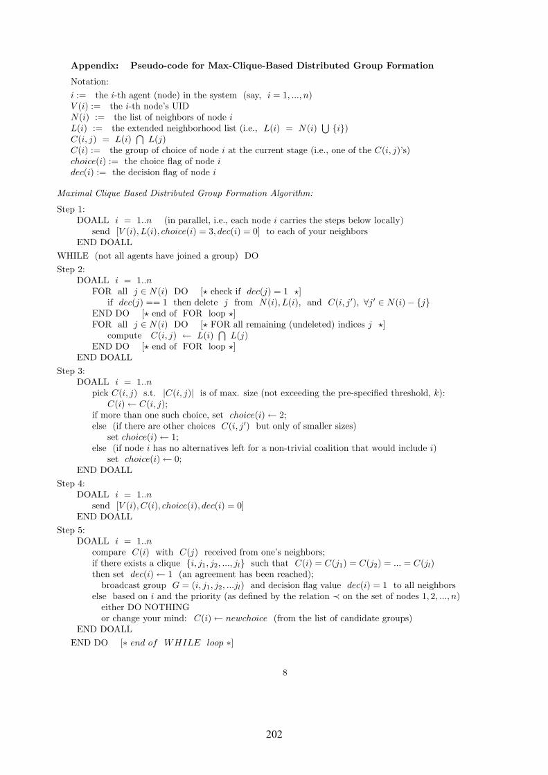
Appendix: Pseudo-code for Max-Clique-Based Distributed Group Formation

Notation:i := the i-th agent (node) in the system (say, i = 1, ..., n)V (i) := the i-th node’s UIDN(i) := the list of neighbors of node iL(i) := the extended neighborhood list (i.e., L(i) = N(i)

⋃i)

C(i, j) = L(i)⋂

L(j)C(i) := the group of choice of node i at the current stage (i.e., one of the C(i, j)’s)choice(i) := the choice flag of node idec(i) := the decision flag of node i

Maximal Clique Based Distributed Group Formation Algorithm:

Step 1:DOALL i = 1..n (in parallel, i.e., each node i carries the steps below locally)

send [V (i), L(i), choice(i) = 3, dec(i) = 0] to each of your neighborsEND DOALL

WHILE (not all agents have joined a group) DOStep 2:

DOALL i = 1..nFOR all j ∈ N(i) DO [? check if dec(j) = 1 ?]

if dec(j) == 1 then delete j from N(i), L(i), and C(i, j′), ∀j′ ∈ N(i)− jEND DO [? end of FOR loop ?]FOR all j ∈ N(i) DO [? FOR all remaining (undeleted) indices j ?]

compute C(i, j) ← L(i)⋂

L(j)END DO [? end of FOR loop ?]

END DOALLStep 3:

DOALL i = 1..npick C(i, j) s.t. |C(i, j)| is of max. size (not exceeding the pre-specified threshold, k):

C(i)← C(i, j);if more than one such choice, set choice(i)← 2;else (if there are other choices C(i, j′) but only of smaller sizes)

set choice(i)← 1;else (if node i has no alternatives left for a non-trivial coalition that would include i)

set choice(i)← 0;END DOALL

Step 4:DOALL i = 1..n

send [V (i), C(i), choice(i), dec(i) = 0]END DOALL

Step 5:DOALL i = 1..n

compare C(i) with C(j) received from one’s neighbors;if there exists a clique i, j1, j2, ..., jl such that C(i) = C(j1) = C(j2) = ... = C(jl)then set dec(i)← 1 (an agreement has been reached);

broadcast group G = (i, j1, j2, ...jl) and decision flag value dec(i) = 1 to all neighborselse based on i and the priority (as defined by the relation ≺ on the set of nodes 1, 2, ..., n)

either DO NOTHINGor change your mind: C(i)← newchoice (from the list of candidate groups)

END DOALLEND DO [∗ end of WHILE loop ∗]

8

202

ATSpace: A Middle Agent to Support Application OrientedMatchmaking and Brokering Services

Myeong-Wuk Jang, Amr Abdel Momen, Gul AghaDepartment of Computer Science

University of Illinois at Urbana-Champaign, USAmjang, amrmomen, agha@uiuc.edu

http://osl.cs.uiuc.edu

Abstract

An important problem for agents in open multiagentsystems is how to find agents that match certain criteria.A number of middle agent services–such as matchmakingand brokering services–have been proposed to address thisproblem. However, the search capabilities of such ser-vices are relatively limited since the match criteria theyuse are relatively inflexible. We propose ATSpace, a modelto support application-oriented matchmaking and broker-ing services. Application agents in ATSpace deliver theirown search algorithms to a public tuple space which holdsagent property data; the tuple space executes the search al-gorithms on this data. We show how the ATSpace modelincreases the dynamicity and flexibility of a middle agentservice. Unfortunately, the model also introduces securitythreats: the data and access control restrictions in ATSpacemay be compromised, and system availability may be af-fected. We describe some mechanisms to address these se-curity threats.

1 Introduction

In multiagent systems, agents need to communicate witheach other to accomplish their goals, and an important prob-lem in open multiagent systems is the problem of findingother agents that match given criteria, called the connectionproblem [4]. When agents are designed or owned by thesame organization, developers may be able to design agentswhich explicitly know the names of other agents that theyneed to communicate with. However in open systems, be-cause an agent may be implemented by different groups, itis not feasible to let agents know the names of all agentsthat they may at some point need to communicate with.

Decker classifies middle agent services as either match-making (also called Yellow Page) services or brokering ser-

vices [5]. Matchmaking services (e.g. Directory Facilitatorin FIPA platforms [7]) are passive services whose goal is toprovide a client agent with a list of names of agents whoseproperties match its supplied criteria. The agent may latercontact the matched agents to request services. On the otherhand, brokering services (e.g. ActorSpace [1]) are activeservices that directly deliver a message (or a request) to therelevant agents on their client’s behalf.

In both types of services, an agent advertises itself bysending a message which contains its name and a descrip-tion of its characteristics to a service manager. A servicemanager may be implemented on top of a tuple space modelsuch as Linda [3]; this involves imposing constraints on theformat of the stored tuples and using Linda-supported prim-itives. Specifically, to implement matchmaking and broker-ing services on top of Linda, a tuple template may be usedby the client agent to specify the matching criteria. How-ever, the expressive power of a template is very limited; itconsists of value constraints for its actual parameters andtype constraints for its formal parameters. In order to over-come this limitation, Callsen’s ActorSpace implementationused regular expressions in its search template [1]. Eventhough this implementation increased expressivity, its capa-bility is still limited by the power of its regular expressions.

We propose ATSpace1 (Active Tuple Spaces) to em-power agents with the ability to provide arbitraryapplication-oriented search algorithms to the tuple spacemanager for execution on the tuple space. While ATSpaceincreases the dynamicity and flexibility of the tuple spacemodel, it also introduces some security threats as codes de-veloped by different groups with different interests are exe-cuted in the same space. We will discuss the implication ofthese threats and how they may be mitigated.

1We will use ATSpace to refer the model for a middle agent to supportapplication-oriented service, while we use an atSpace to refer an instanceof ATSpace.

203

2 ATSpace

2.1 A Motivativing Example

We present a simple example to motivate the ATSpacemodel. Assume that a tuple space has information aboutseller agents (e.g., city and name) and the prices of the prod-ucts they sell. A buyer agent wants to contact the two “best”seller agents who offer computers and whose location iswithin 50 miles of his city. A brokering service supplied bya generic tuple space implementation may not support therequest of the buyer agent because, firstly, it may not sup-port the “best two” primitive, and secondly, it may not storedistance information between cites. The buyer agent is nowopt to retrieve from the tuple space the complete tuples thatare related to computer sellers, and then execute their ownsearch algorithm on them. However, this approach entailsthe movement of large amount of data. In order to reducecommunication overhead, ATSpace allows a sender agentto send its own search algorithm which may, for example,carry information about distances to the nearest cities.

2.2 Overall Architecture

ATSpace consists of three components: a tuple space, amessage queue, and a tuple space manager (see Figure 1).

ATSpace

Tuple Space

Message Queue

TupleSpaceManager

(matchmaking)return names

ask service agents(brokering)

tuple

tuple

tuple

tuplemsg.msg. msg.

Figure 1. Basic Architecture of ATSpace

The tuple space is used as a shared pool for agent tuples,〈a, p1, p2, . . . , pn〉, which consists of a name field, a, anda property part, P = p1, p2, · · · , pn where n ≥ 1; eachtuple represents an agent whose name is given by the firstfield and whose characteristics are given by the subsequentfields. ATSpace enforces the rule that there cannot be morethan one agent tuple whose agent names and property fieldsare identical at any time. However, an agent may regis-ter itself with different properties, and different agents mayregister themselves with the same property fields.

∀ti, tj : i = j → [ (ti.a = tj .a) → (ti.p = tj .p) &&(ti.p = tj .p) → (ti.a = tj .a) ]

The message queue contains input messages that are re-ceived from other agents. Messages are classified into twotypes: data input messages and service request messages. Adata input message includes a new agent tuple for insertioninto the tuple space. A service request message includes ei-ther a tuple template or a mobile object. The template (or,alternately, the object) is used to search for agents with theappropriate agent tuples. A service message may optionallycontain another field, called the service call message field,to facilitate the brokering service. A mobile object is an ob-ject that is provided by a service request agent; such objectshave a pre-defined public method called find. The findmethod is called by the tuple space manager with tuples inthis atSpace as a parameter; it returns names of agents se-lected by the search algorithm specified in the mobile ob-ject.

The tuple space manager retrieves names of serviceagents whose properties match a tuple template or whichare selected by the mobile object. In case of a matchmak-ing service, it returns the names to the client agent. In caseof brokering service, it forwards the service call messagesupplied by the client agent to the agents.

2.3 Operation Primitives

The ATSpace model supports the three general tuplespace primitives: write, read, and take. In addi-tion, ATSpace also provides primitives for the matchmak-ing and brokering services. The searchOne primitiveis used to retrieve the name of a service agent that satis-fies a given property, whereas the searchAll primitive isused to retrieve the names of all service agents that satisfythe property. The deliverOne primitive is used to for-ward a specified message to a service agent that matchesthe property, whereas the deliverAll is used to sendthis message to all such service agents. These matchmak-ing and brokering service primitives allow client agents touse mobile objects to support application-oriented searchalgorithm as well as a tuple template. MobileObject isused as an abstract class that defines the interface methodsbetween a mobile object and the ATSpace. One of thesemethods is find, which may be used to provide the searchalgorithm to an atSpace.

When a client agent requires information about specificproperties of service agents stored in an atSpace to makeservice call messages, the above matchmaking or broker-ing service primitives cannot be used. The exec primitivewithin a mobile object provides this service. The suppliedmobile object has to implement the doAction methodwhich when called by the atSpace with agent tuples, exam-ines the properties of agents using the client agent applica-tion logic, creates different service call messages accordingto the properties, and then returns a list of agent messages

204

to the atSpace for delivery to the selected agents.

3 Security Issues

There are three important security problems in ATSpace.

Data Integrity A mobile object may not modify tuplesowned by other agents.

Denial of Service A mobile object may not consume toomuch processing time or space of an atSpace and aclient agent may not send repeatedly mobile objectsto overload an atSpace.

Illegal Access A mobile object may not carry out unautho-rized accesses or illegal operations.

We address the data integrity problem by blocking at-tempts to modify tuples. When a mobile object is executedby a tuple space manager, the manager makes a copy of tu-ples and then sends the copy to the find or doActionmethod of the mobile object. Therefore, even when a mali-cious agent changes some tuples, the original tuples are notaffected by the modification. However, when the number oftuples in the tuple space is very large, this solution requiresextra memory and computational resources. For better per-formance, the creator of an atSpace may select the optionto deliver a shallow copy of the original tuples to mobileobjects instead of a deep copy, although this will violate theintegrity of tuples if an agent tries to delete or change itstuple. We are currently investigating under what conditionsa use of a shallow copy may be sufficient.

To address denial of service by consuming all processorcycles, we deploy user-level thread scheduling. Figure 2depicts the extension of the tuple space manager to achievethis. When a mobile object arrives, the object is executedas a thread, and its priority is set to high. If the thread exe-cutes for a long time, its priority is continually downgraded.Moreover, if the running time of a mobile object exceeds acertain limit, it may be destroyed by the Tuple Space Man-ager; in this case, a message is sent to its supplier informingit of the destruction. To incorporate these restrictions, wehave extended the architecture of ATSpace by implement-ing job queues.

To prevent unauthorized accesses, if an atSpace is cre-ated with an access key, then this key must accompany ev-ery message sent from service requester agents. In this case,agents are allowed to modify only their own tuples. Thisprevents removal or modification of tuples by unauthorizedagents.

4 Evaluation

Figure 3 shows the advantage of ATSpace compared toa matchmaking service which provides the same semantic

Tuple Space Manager

priority

job queues

priorityhigh

priority

low

middle

ATSpaceManager obj.obj.

obj.obj.

obj.obj.

Figure 2. Extended Architecture of ATSpace

in UAV simulation (see [9] for details of this simulation).In these experiments, the UAVs use either an active broker-ing service or a matchmaking service to find their neighbor-ing UAVs. In both cases, the middle agent includes infor-mation about the locations of UAVs. In case of the activebrokering service, UAVs send mobile objects to the middleagent while UAVs using matchmaking service send tupletemplates. The simulation time for each run is around 35minutes.

0

100

200

300

400

500

600

200 300 400 500 600 700 800 900 1000

Wal

l Clo

ck T

ime

(min

)

Number of Agents

ATSpaceMatchmaking

Figure 3. Wall Clock Time for ATSpace andMatchmaking Services

When the number of agents is small, the difference be-tween the two approaches is not significant. However, asthe number of agents is increased, the difference becomessignificant.

5 Related Work

Our work is related to Linda [3] and its variations, suchas JavaSpaces and TSpaces [10, 13]. In these models, pro-cesses communicate with other processes through a sharedcommon space called a tuple space without considering ref-

205

erences or names of other processes. From the middle agentperspective, Directory Facilitator in the FIPA platform andBroker Agent in InfoSleuth are related to our research [7, 8].However, these systems do not support customizable match-ing algorithm.

Some work has been done to extend the matching ca-pability in the tuple space model. Berlinda allows a con-crete entry class to extend the matching function [14]. How-ever, this approach does not allow the matching function tobe changed during execution time. OpenSpaces provides amechanism to change matching polices during the execu-tion time [6]. OpenSpaces groups entries in its space intoclasses and allows each class to have its individual match-ing algorithm. A manager for each class of entries canchange the matching algorithm during execution time. Allagents that use entries under a given class are affected byany change to its matching algorithm. This is in contrastto ATSpace where each agent can supply its own matchingalgorithm without affecting other agents. Another differ-ence between OpenSpaces and ATSpace is that the formerrequires a registration step before putting the new matchingalgorithm into action.

TuCSoN and MARS provide programmable coordinationmechanisms for agents through Linda-like tuple spaces toextend the expressive power of tuple spaces [2, 11]. How-ever, they differ in the way they approach the expressivenessproblem; while TuCSoN and MARS use reactive tuples toextend the expressive power of tuple spaces, ATSpace usesmobile objects to support search algorthms defined by clientagents. A reactive tuple handles a certain type of tuples andaffects various clients, whereas a mobile object handles var-ious types of tuples and affects only its creator agent. Also,these approaches do not provide an execution envrionmentfor client agents. Therefore, these may be considered asorthogonal approaches and can be combined with our ap-proach together.

6 Conclusion

ATSpace works as a common shared space to exchangedata among agents, a middle agent to support matchmak-ing and brokering services, and an execution environmentfor mobile objects utilizing data on its space. Our exper-iments with a UAV surveillance task show that the modelmay be effective in reducing coordination costs. We de-scribed some security threats that arise when using mobileobjects for agent coordination, along with some mecha-nisms we use to mitigate them. We are currently incor-porating memory use restrictions into the architecture andconsidering mechanisms to address denial of service attacksthat may be caused by flooding the network [12].

Acknowledgements

This research is sponsored by the DARPA ITO undercontract number F30602-00-2-0586.

References

[1] G. Agha and C. Callsen. ActorSpaces: An Open DistributedProgramming Paradigm. In Proceedings of the 4th ACMSymposium on Principles & Practice of Parallel Program-ming, pages 23–32, May 1993.

[2] G. Cabri, L. Leonardi, and F. Zambonelli. MARS: a Pro-grammable Coordination Architecture for Mobile Agents.IEEE Computing, 4(4):26–35, 2000.

[3] N. Carreiro and D. Gelernter. Linda in Context. Communi-cations of the ACM, 32(4):444–458, 1989.

[4] R. Davis and R. Smith. Negotiation as a Metaphor for Dis-tributed Problem Solving. Artificial Intelligence, 20(1):63–109, January 1983.

[5] K. Decker, M. Williamann, and K. Sycara. Matchmak-ing and Brokering. In Proceedings of the Second Interna-tional Conference on Multi-Agent Systems (ICMAS-96), Ky-oto, Japan, December 1996.

[6] S. Ducasse, T. Hofmann, and O. Nierstrasz. OpenSpaces:An Object-Oriented Framework for Reconfigurable Coordi-nation Spaces. In A. Porto and G. Roman, editors, Coor-dination Languages and Models, LNCS 1906, pages 1–19,Limassol, Cyprus, September 2000.

[7] Foundation for Intelligent Physical Agents. SC00023J:FIPA Agent Management Specification, December 2002.http://www.fipa.org/specs/fipa00023/.

[8] N. Jacobs and R. Shea. The Role of Java in InfoS-leuth: Agent-based Exploitation of Heterogeneous Informa-tion Resources. In Proceedings of Intranet-96 Java Devel-opers Conference, April 1996.

[9] M. Jang, A. A. Momen, and G. Agha. A Flexible Coordina-tion Framework for Application-Oriented Matchmaking andBrokering Services. Technical Report UIUCDCS-R-2004-2430, Department of Computer Science, University of Illi-nois at Urbana-Champaign, 2004.

[10] T. Lehman, S. McLaughry, and P. Wyckoff. TSpaces: TheNext Wave. In Proceedings of the 32nd Hawaii Interna-tional Conference on System Sciences (HICSS-32), January1999.

[11] A. Omicini and F. Zambonelli. TuCSoN: a CoordinationModel for Mobile Information Agents. In Proceedings of the1st Workshop on Innovative Internet Information Systems,Pisa, Italy, June 1998.

[12] C. Shields. What do we mean by Network Denial of Ser-vice? In Proceedings of the 2002 IEEE Workshop on Infor-mation Assurance and Security, pages 17–19, United StatesMilitary Academy, West Point, NY, June 2002.

[13] Sun Microsystems. JavaSpacesTM Service Specification,ver. 2.0, June 2003. http://java.sun.com/products/jini/specs.

[14] R. Tolksdorf. Berlinda: An Object-oriented Platform forImplementing Coordination Language in Java. In Proceed-ings of COORDINATION ’97 (Coordination Languages andModels), LNCS 1282, pages 430–433. Pringer-Verlag, 1997.

206

Learning Continuous Time Markov Chains from Sample ExecutionsKoushik Sen, Mahesh Viswanathan, Gul Agha

Department of Computer ScienceUniversity of Illinois at Urbana Champaignksen,vmahesh,agha @cs.uiuc.edu

AbstractContinuous-time Markov Chains (CTMCs) are an impor-

tant class of stochastic models that have been used to modeland analyze a variety of practical systems. In this paper wepresent an algorithm to learn and synthesize a CTMC modelfrom sample executions of a system. Apart from its theoret-ical interest, we expect our algorithm to be useful in veri-fying black-box probabilistic systems and in composition-ally verifying stochastic components interacting with un-known environments. We have implemented the algorithmand found it to be effective in learning CTMCs underlyingpractical systems from sample runs.

1. IntroductionStochastic models such as continuous-time Markov

chains (CTMCs) [22] are widely used to model prac-tical software systems and analyze their performanceand reliability. Before building a complex software sys-tem, CTMCs are generated from higher-level speci-fications, like queueing networks, stochastic processalgebra [14, 11], or stochastic Petri-nets [4]. These mod-els are then used for quantitative evaluation of reliabilityand performance for example to determine the through-put of production lines, to calculate average failure timeof systems, or to find other reliability or performance bot-tlenecks of the system. Once a model has been validatedagainst performance and reliability requirements, the sys-tem is implemented. However, even if a model has beencarefully validated, the implementation may not con-form to the model. There are two potential sources oferror: first, there could be bugs introduced when trans-lating the design into system code, and second the es-timated values of various parameters used in construct-ing the stochastic model may differ considerably from theactual values in the deployed system. To catch such po-tential post-implementation problems, testing for perfor-mance and reliability is performed by running the system alarge number of times in the real environment and check-ing for reliability problems or performance bottlenecks.However, because it is difficult achieve completecover-ageduring testing, despite its evident importance in prac-tice, testing fails to guarantee the full correctness of adeployed system.

An approach that tries to leverage the benefits of formalanalysis - usually done in the design phase - to the post-implementation phase, islearning the model from sam-ple executions of the system and then formally verifyingthe learnt model against the design specification. This ap-proach has been fruitfully used to model-check unknown,black-boxsystems [9] and to learn unknown environmentsto assist in compositional verification of systems [7]. Boththese efforts apply to non-deterministic, discrete systemsand have not been extended to more general stochastic sys-tems. While there are several machine learning algorithmson grammatical inference [6, 1, 8, 19, 5] that have beensuccessfully applied to pattern recognition, speech recog-nition, natural language processing and several other do-mains, there are no algorithms in the literature that can learnthe real-time, stochastic models that are typically used tomodel systems in formal verification. In this paper, we ad-dress this problem by presenting an algorithm that given ex-ecution traces (possibly obtained by running the deployedsystem during testing) of the system, infers a CTMC modelthat could have generated the traces according to the ob-served distribution. The learned CTMC can then be usedby existing probabilistic model-checking [17, 12, 21, 24]and performance evaluation tools [14, 4] for further analy-sis and thereby helping to find bugs in post-implementationphase. The learning algorithm may also potentially be usedto perform automatic compositional verification (as in [7])for stochastic systems. A closely related work is given in[23] where they learn continuous-time hidden Markov mod-els to do performance evaluation. However, they fix the sizeof the continuous-time hidden Markov model before learn-ing. This can be restrictive if the system cannot be modelledby a continuous-time hidden Markov model of given size.In our approach there is no such restriction.

We present an algorithm and show that it correctly iden-tifies the CTMC model in the limit [8] when it is givensamples drawn from a distribution generated by a CTMC.One technical difficulty when talking about samples drawnfrom a CTMC is that traditionally CTMCs are unlabeled,and so they only have runs, which are sequences of statesthat are traversed and not traces. However, the problem isthat when samples are drawn from an implementation get-

1

207

ting information that uniquely identifies states is expensiveand impractical, and can lead to the construction of a verylarge model which does not collapse equivalent states. Toaddress this difficulty, we introduce the model of anEdgeLabeled Continuous-time Markov Chain(CTMCL) whereedges are labeled from a finite set of alphabet and traces aresequences of edge labels which are given to the learning al-gorithm.

Our algorithm is based on the state merging paradigmintroduced and used in RPNI [19] and ALERGIA [6]. Thesamples provided to the learning algorithm are used to con-struct what we call aprefix-tree continuous-time Markovchain. Such Markov chains are the simplest CTMC that areconsistent with the samples. The algorithm then progres-sively generalizes this model (i.e., produces models with ad-ditional behaviors) by merging pairs of states about whose“equivalence” the sample has evidence. Since the tracesdo not have complete state information about the originalCTMC states, statistical information present in the samplesis used to distinguish states. Our key algorithmic insight isin determining the statistical tests that can be used to con-clude the equivalence of states with a given confidence. Thecandidate states that are tested for equivalence by the algo-rithm are done in a carefully chosen order (as in RPNI andALERGIA) to ensure that the algorithm runs in time poly-nomial in sample size. The algorithm terminates when ithas tested for all possible merges. Like all algorithms thatlearn in the limit, we show that this algorithm learns the cor-rect CTMC given a sufficiently large sample. Our proof thatthe algorithm learns in the limit relies on a novel methodto bound the error probability of our statistical tests. TheCTMC that the algorithm learns may be much smaller thanthe implementation, since it merges all potentially equiva-lent states, and it only generates thereachableportion of theimplementation. This can be particularly beneficial in thecontext of formal verification; the running time and spacerequirements of verification algorithms depend on the sizeof the reachable portion of the model. We have implementedour algorithm in Java and experimented by learning someexample systems encountered in practice.

The rest of the paper is organized as follows. We givethe preliminary definitions and notations in Section 2, fol-lowed by the learning algorithm in Section 3. In Section 4we prove that the learned CTMC converges to the originalCTMC in the limit. We report our initial experimental re-sults in Section 5 and conclude in Section 6.2. Preliminaries

We recall some basic concepts related to CTMCs. Ourpresentation of this material is slightly non-standard in thatwe consider CTMCs that have labels both on the edges andthe states. In what follows we assumeAP to be a finite setof atomic propositions that are used in describing reliabilityand performance constraints.

Definition 1 An Edge Labeled Continuous-time MarkovChain(CTMCL) is a tupleM = (S, Σ, s0, δ, ρ, L) where

• S is a finite set of states,

• Σ is a finite alphabet of edge labels,

• s0 ∈ S is the initial state,

• δ : S×Σ → S is a partial function which maps a stateand an alphabet to the next state,

• ρ : S × Σ → R≥0 is a function which returns a posi-tive real, calledrate, associated with the transition. Weassume thatρ(s, a) = 0 if and only ifδ(s, a) is not de-fined.

• L : S → 2AP is a function which assigns to each states ∈ S the setL(s) of atomic propositions that are validin s.

A CTMCL defined as above is deterministic in the sensethat for a given states ∈ S and an alphabeta ∈ Σ thestate reached froms by the edge labeleda is unique if itexists. Intuitively, the probability of moving from statesto states′ along the edge labeleda within time t is givenby (1 − e−ρ(s,a)t). This probability corresponds to the cu-mulative probability of an exponential distribution with rateρ(s, a). For a given states, if there are more than one al-phabeta ∈ Σ such thatρ(s, a) > 0 then there is a competi-tion between the transitions. More precisely, for each tran-sition s → δ(s, a) from s for which ρ(s, a) > 0, a ran-dom time t is sampled from the exponential distributionwith rateρ(s, a). Then the transition corresponding to thelowest sampled time is taken. The probability to move froma states to another state, along the edgea, within t timeunits i.e. the time sampled for the transition correspondingto s → δ(s, a) is minimum, is given by

P(s, a, t) =ρ(s, a)E(s)

(1− e−E(s)t

)

where E(s) =∑

a∈Σ ρ(s, a) is the total rate at whichany transition from the states is taken. In other words,the probability of leaving the states within t time units is(1 − e−E(s)t). This is because the distribution for the min-imum time among all edges is exponential with rateE(s).Thus we can see the probability of moving from a statesalong the edgea is the probability of staying at the statesfor less thant time units times the probability of taking theedgea. The probability of taking the edgea from states isthus given by

P(s, a) =ρ(s, a)E(s)

WhenE(s) = 0, we defineP(s, a) = 0 for everya.

2

208

Paths and Probability SpaceA pathτ starting at states is

a finite or infinite sequencel0(a1,t1)−→ l1

(a2,t2)−→ l2(a3,t3)−→ · · ·

such that there is a corresponding sequencev0a1−→ v1

a2−→v2

a3−→ · · · of states withs = v0, L(vi) = li, ti ∈ R≥0,δ(vi, ai+1) = vi+1 for all i. For a pathτ from s, τ [s, i] = vi

is the ith state of the path andη[τ, s, i] = ti is the timespent in statevi−1. A maximalpath starting at states is apath τ starting ats such that it is either infinite or (if fi-nite)E(τ [s, n]) = 0, wheren is the length ofτ . The set ofall maximal paths starting at states is denoted byPath(s);the set of all (maximal) paths in a CTMCM, denoted byPath(M), is taken to bePath(s0), wheres0 is the initialstate.

Let π = l0a1−→ l1

a2−→ · · · ak−→ lk be a finite sequencesuch that there is a sequence of statess0, s1, . . . sk suchthat s0 is the initial state,L(si) = li and δ(si, ai+1) =si+1; π[i] is used to denote statesi in the sequence cor-responding toπ. Let I1, I2, . . . Ik be non-empty intervalsin R≥0. Then C(l0, (a1, I1), l1, . . . (ak, Ik), lk) denotes acylinder setconsisting of all pathsτ ∈ Path(s0) such thatτ [s0, i] = π[i] (for i ≤ k) andη[τ, s0, i] ∈ Ii. Let B bethe smallestσ-algebra onPath(s0) which contains all thecylindersC(l0, (a1, I1), l1, . . . (ak, Ik), lk). The probabilitymeasure overB is the unique measure inductively definedasPath(C(l0)) = 1, if L(s0) = l0 and fork > 0 as

Prob(C(l0, (a1, I1), l1, . . . lk−1, (ak, Ik), lk))= Prob(C(l0, (a1, I1), l1, . . . lk−1))·

P(sk−1, ak) · (e−E(sk−1)` − e−E(sk−1)u)

where` = inf Ik andu = sup Ik, andsk−1 = π[k − 1]

3. Learning Edge Labeled CTMCsThe learning problem considered in this paper falls un-

der the category of stochastic grammatical inference [6, 16,20, 5]. In stochastic grammatical inference, samples aretaken from a stochastic language. Given these samples thestochastic language is learned by finding statistical regular-ity among the samples. The parameters for the different dis-tributions determining the language are also estimated fromthe relative frequencies of the samples. For most of theselearning algorithms it has been shown that they can learnthe stochastic language in thelimit i.e. if the number of sam-ples tends towards infinity then the learned language is thesame as the language that generated the sample. All these al-gorithms essentially follow the same technique: they builda prefix-tree automata which stores exactly the same sam-ples and then they test and merge possibly equivalent states.

We present the algorithm for learning edge labeledCTMCs. We first consider the issue of how to gener-ate and reason about behaviors (visible execution traces) offinite length, given that traditionally the behaviors are as-sumed to be of infinite length. We then present some con-cepts that are used in the algorithm. After this we present

the algorithm, whose proof of correctness appears in Sec-tion 4.

3.1. Generating SamplesIn this paper we consider the problem of learning

CTMCL from examples generated by simulating a sys-tem under investigation. The wayCTMCL is formallydefined in Section 2, all behaviors aremaximal execu-tions, and maximal executions are typically infinite. Thiscreates a technical difficulty namely what the samples ap-propriate for learning are. To overcome this problemwe define a finitary version ofCTMCL called Fini-tary Edge Labeled Continuous-time Markov Chains(CTMC f

L) which is a CTMCL, with a non-zero stop-ping probability in any state. This allows one to generateand reason about behaviors of finite length. It is impor-tant to note however, that use ofCTMC f

L is merely atechnical tool. Our primary goal is to learn the under-lying CTMCL and as we shall see in Proposition 3,we can achieve this by learning theCTMC f

L. More-over in this effort, the specific value of the stoppingprobability that we use does not influence the correct-ness of the result. We present the formal definition of aCTMC f

L.

Definition 2 A Finitary Edge Labeled Continuous-timeMarkov Chain(CTMC f

L) is a pair F = (M, p) whereM is a CTMCL and p denotes the stopping probabil-ity in any states ofMThere exists a trivial surjectionΘ: (M, p) 7→ M.

A finite sequenceτ = l0(a1,t1)−→ l1

(a2,t2)−→ l2 · · · (an,tn)−→ lnis a path of theCTMC f

L F = (M, p) starting from a statesiff it is path (not necessarily maximal) ofM starting froms.The set of paths starting from states is denoted byPath(s).The ith state of pathτ from s and the time spent in theith state are defined similarly, and are denoted byτ [s, i]and η[τ, s, i], respectively.Theσ-field corresponding to aCTMC f

L is defined analogously to that of aCTMCL. Forthe pathτ from states, the probability that theCTMC f

L ex-hibits such a path is given by

ProbF (τ, s) =(1− p) ·P(τ [s, 0], a1, t1) · (1− p) ·P(τ [s, 1], a2, t2)· · · (1− p) ·P(τ [s, n− 1], an, tn) · p

Given aCTMCL we extend it to aCTMC fL by associat-

ing a known probabilityp⊥ (say p⊥ = 0.1) as the stop-ping probability. TheCTMC f

L thus obtained is then simu-lated to get a multi-set of finite samples which we treat asthe multi-set of examples for learning. In our algorithm wewill assume that we are given a finite multi-set of examplesfrom aCTMCL M extended with a known stopping prob-ability p to aCTMC f

L. Our goal will be to learnM fromthe multi-set of examples.

3

209

Note that for a given implemented system, which can beseen as a software program, an example can be generatedin the following way. Lets0 be the initial state of the pro-gram. Then addl0 = L(s0) to the example sequence. We seta probabilityp0 = 0.1. With probabilityp0 return the cur-rent sequence as an example. With probability1 − p0 ex-ecute the next instruction of the program. If the executionof the instructionai takes timeti and results in the change

of state fromsi−1 to si then add(ai,ti)−→ L(si) to the exam-

ple sequence.

3.2. DefinitionsWe next define the notations and the concepts that

we will use to describe the learning algorithm. Given aCTMCL M = (S, Σ, s0, δ, ρ, L) we can extend the defini-tion of δ as follows:

δ(s, λ) = s whereλ is the empty stringδ(s, xa) = δ(δ(s, x), a) wherex ∈ Σ∗ anda ∈ Σδ(s, a) = ⊥ if δ(s, a) is not definedδ(s, xa) = ⊥ if δ(s, x) = ⊥ or δ(δ(s, x), a) is undefined

For a given exampleτ = l0(a1,t1)−→ l1

(a2,t2)−→ l2 · · · (an,tn)−→ln, let τ |Σ be the stringa1a2 . . . an. We usePr(τ) to de-note the setx | ∃y : xy = τ |Σ, that is,Pr(τ) is the setof all prefixes ofτ |Σ. Given a multi-setI+ of examples, letPr(I+) be the set

⋃τ∈I+ Pr(τ). If there exists an exam-

ple l0(a1,t1)−→ l1

(a2,t2)−→ l2 · · · (ai,ti)−→ li · · · (an,tn)−→ ln in I+

such thatx = a1a2 . . . ai then we defineL(x, I+) = li.Let n(x, I+) be the number ofτ ∈ I+ such thatx ∈

Pr(τ) and letn′(x, I+) ben(x, I+) minus the number ofx ∈ I+. Thus n(x, I+) counts the number of examplesin I+ for which x is a prefix andn′(x, I+) is the num-ber of examples inI+ for which x is prefix and length of

x is less than the length of the example. Forτ = l0(a1,t1)−→

l1(a2,t2)−→ l2 · · · (ai,ti)−→ li · · · (an,tn)−→ ln, if x = a1a2 . . . ai−1

anda = ai, thenθ(x, a, τ) = ti and0 otherwise; in otherwords,θ(x, a, τ) denotes the time spent in the state reachedafterx in τ . We defineθ(x, I+) andp(x, a, I+) as follows:

θ(x, I+) =

∑a∈Σ

∑τ∈I+ θ(x,a,τ)

n′(x,I+) if n′(x, I+) > 00 otherwise

p(x, a, I+) =

n(xa,I+)n′(x,I+) if n′(x, I+) > 00 otherwise

Note thatθ(x, I+) gives an estimate of1/E(s) wheres is the stateδ(s0, x) and p(x, a, I+) gives an estimate ofP(s, a).

Given a multi-setI+ of examples we first construct aprefix-treeCTMC f

L defined as follows.

Definition 3 The prefix-tree CTMC fL for a multi-

set of examplesI+ is a CTMC fL PCTMC (I+) =

((S, Σ, s0, δ, ρ, L), p), where

1. S = Pr(I+)

2. s0 = λ (the empty string)

3. δ(x, a) =

xa if xa ∈ S⊥ otherwise

4. E(x) = 1/θ(x, I+)

5. P(x, a) = p(x, a, I+)

6. ρ(x, a) = P(x, a)E(x)

7. L(x) = L(x, I+)

8. p is the stopping probability associated with theCTMC f

L that generated the examples.

A PCTMC (I+) is anCTMC fL consistent with the ex-

amples inI+ in the sense that for every example inI+ thereis a corresponding path in theCTMC f

L.The learning algorithm proceeds by generalizing the ini-

tial guess,PCTMC (I+), by mergingequivalentstates. Theformal definition of when two states are equivalent is nowpresented.

Definition 4 Given aCTMCL M = (S, Σ, s0, δ, ρ, L), arelationR ⊆ S × S is said to bestable relationif and onlyif for anys, s′ ∈ S such that(s, s′) ∈ R, we have

a) L(s) = L(s′)

b) E(s) = E(s′)

c) for all a ∈ Σ if there existst ∈ S such thatδ(s, a) = tthen there exists at′ ∈ S such thatδ(s′, a) = t′,P(s, a) = P(s′, a) and(t, t′) ∈ R, and conversely

d) for all a ∈ Σ if there existst′ ∈ S such thatδ(s′, a) =t′ then there exists at ∈ S such thatδ(s, a) = t,P(s′, a) = P(s, a) and(t′, t) ∈ R.

Two statess ands′ in CTMCL M are said to beequivalent(s ≡ s′) if and only if there is a stable relationR such that(s, s′) ∈ R.

The correctness of learning algorithm crucially dependson the fact that merging two equivalent states results in aCTMCL that generates the same distribution. But beforewe state and prove this formally we make a simple observa-tion about equivalent states.

Lemma 1 Let F = (M, p) be anCTMC fL and s ≡ s′.

τ is a path starting froms iff τ is a path starting froms′.MoreoverProbF (τ, s) = ProbF (τ, s′).

Proof: Let τ = l0(a1,t1)−→ l1

(a2,t2)−→ l2 · · · (an,tn)−→ ln be a pathstarting froms. There is a sequencev0

a1−→ v1a2−→ · · · vn

of states such thatv0 = s. Sinces ≡ s′ andδ(s, a1) = v1,there must be a stateu1 such thatδ(s′, a1) = u1 andu1 ≡ v1. Continuing inductively, we can construct a se-quence of statesu0

a1−→ u1a2−→ · · ·un, such thatu0 = s′

4

210

andui ≡ vi. Henceτ is also a path starting froms′. Fur-thermore, sinceui ≡ vi, we know thatE(ui) = E(vi),andP(ui, ai+1) = P(vi, ai+1) and henceProbF (τ, s) =ProbF (τ, s′). For paths starting froms′, the argument issymmetric.

Definition 5 TwoCTMC fLsF andF ′ with initial statess0

ands′0, respectively, are said to beequivalentif Path(F) =Path(F ′) and for everyτ ∈ Path(F), ProbF (τ, s0) =ProbF ′(τ, s′0).

For a CTMCL M = (S, Σ, s0, δ, ρ, L), the minimalCTMCL is defined to be the quotient ofM with respectto the equivalence relation on states. Formally, the minimalCTMCL isM′ = (S′, Σ, s′0, δ

′, ρ′, L′) such that

1. S′ are the equivalence classes ofS with respect to≡,

2. s′0 = [s0], the equivalence class ofs0

3. δ′([s], a) = [s′] iff δ(s, a) = s′

4. ρ′([s], a) = ρ(s, a) and

5. L′([s]) = L(s)

Observe, that this is well-defined, because of the way≡ isdefined.

Proposition 2 Let F = (M, p) be a CTMC fL. Then

F ′ = (M′, p) is equivalent toF whereM′ is the mini-malCTMCL corresponding toMProof: The proof is a straightforward consequence of thedefinition of the minimalCTMCL M′. It relies on the ob-servation that for a pathτ , v0

a1−→ v1a2−→ · · · vn is a se-

quence of states visited inM iff [v0]a1−→ [v1]

a2−→ · · · [vn]in M′. Furthermore, sinceρ′([s], a) = ρ(s, a), the proba-bilities are also the same.

We conclude the section with the observation that forequivalentCTMC f

Ls with the same stopping probability,the associatedCTMCLs define the same probability spaceon the set of paths. This next proposition together withProposition 2 shows that given anyCTMCL, we can al-ways construct a smaller equivalentCTMCL by mergingequivalent states, thus providing mathematical justificationfor our algorithm.

Proposition 3 LetF = (M, p) andF ′ = (M′, p) be twoCTMC f

Ls with the same stopping probabilityp. Then theprobability spaces defined byM andM′ are the same.

We skip the proof of this proposition in the interests ofspace. However, we would like to point out some of the im-portant consequences of Proposition 3. First is that if welearn anCTMC f

L that has the same stopping probability asthe one that was used to generate the samples from the sys-tem, then the underlyingCTMCLs are also equivalent interms of the distribution on traces they generate. Second,the specific value of the stopping probability plays no role

in proving the correctness of our learning algorithm. It mayhave an effect in terms of the length of traces produced andthe number of traces needed to learn. The right choice ofthe stopping probability is thus one that is determined bythe empirical constraints that one is working in.

3.3. Learning Algorithm

algorithm learnCTMCInput: I+ : a multi-set of examples

α : confidence levelOutput: CTMCL

beginA ← PCTMC (I+)for i = 2 to |A| do

for j = 1 to i− 1 doif compatible(si, sj , α, I+) then

A ← merge(A, si, sj)A ← determinize(A)exit j-loop

endifreturn A

endFigure 1. Algorithm to learnCTMC f

L

The algorithm for CTMCL learning, describedin Figure 1, first constructs the prefix-treeCTMC f

L

A = PCTMC (I+) from the multi-set of examplesI+. Weassume that the states inA are ordered in lexicographic or-der.1 Let |A| be the number of states inA. The algorithmthen tries to merge pairs of states inA that are equiva-lent in a quadratic loop, i.e. for alli from 1 to |A| the al-gorithm tries to mergesi with the statess1, s2, . . . , si−1

in that order. If two statessi and sj are equivalent theyare merged using the methodmerge(A, si, sj). The small-est state in a block of merged states is used to represent thewhole block. After every merge of statesi andsj the result-ing CTMC f

L may be non-deterministic. However, equiva-lence ofsi andsj implies that each successor ofsi is equiv-alent to the corresponding successor ofsj . This meansthat those successors should also get merged. To en-sure this the methoddeterminize(A) described in Fig-ure 2 is invoked which removes the non-determinism inA by a sequence of merges. After every merge the prob-abilities P(s, a) and the ratesE(s) are re-computed forevery state as there is more information available at ev-ery state. The algorithm stops when no more merging ispossible.

1 For Σ = a, b, the lexicographic ordering isλ, a, b, aa, ab, ba, bb, aaa, . . .

5

211

algorithm determinizeInput: AOutput: CTMCL

beginwhile(∃s, a ∈ A : s′, s′′ ∈ δ(s, a)) do

A ← merge(A, s′, s′′)return A

endFigure 2. determinizeremoves non-determinism

Now the observations Proposition 2 and 3 together sug-gest that the above algorithm would be correct if indeed wecould test for equivalence of two states. This, however, isnot the case, asA is built from experimental data. However,we approximately check the equivalence of two states recur-sively through statistical hypothesis testing [15, 18]. We saythat two statessi andsj are compatible, denoted bysi ≈ sj ,if L(s) = L(s′), E(s) ∼ E(s′), for all a ∈ Σ, P(si, a) ∼P(sj , a), and δ(si, a) ≈ δ(sj , a), whereE(s) ∼ E(s′)means thatE(s) andE(s′) are equal within some statisticaluncertainty and similarly forP(si, a) ∼ P(sj , a). The deci-sion for compatibility is made using the functioncompatibledescribed in Figure 3.

algorithm compatibleInput: x, y, I+, αOutput: booleanbegin

if L(x, I+) 6= L(y, I+) thenreturn FALSE

if differentExpMeans(θ(x, I+), n′(x, I+),

θ(y, I+), n′(y, I+), α) thenreturn FALSE

for ∀a ∈ Σif differentBerMeans(p(x, a, I+), n(xa, I+),

p(y, a, I+), n(ya, I+), α) thenreturn FALSE

if not compatible(δ(x, a), δ(y, a), I+, α) thenreturn FALSE

endforreturn TRUE

end

Figure 3. compatiblechecks if two two states are ap-proximately equivalent

The check forE(si) ∼ E(sj) is performed by the func-tion differentExpMean, described in Figure 4, which usesstatistical hypothesis testing. The function actually checksif the means1/E(si) and1/E(sj) of two exponential dis-tributions are different. Given two exponential distributionswith meansθ1 andθ2 we want to check ifθ1 = θ2 against

the fact fact thatθ1 6= θ2. This is equivalent to checkingθ1θ2

= 1 against the fact thatθ1θ26= 1. In statistical terms

we call θ1θ2

= 1 as the null hypothesis (denoted byH0)

and θ1θ26= 1 as the alternate hypothesis (denoted byHa).

To test the hypothesisH0 againstHa we drawn1 samples,sayx1, x2, . . . , xn1 , from the exponential distribution withmeanθ1 andn2 samples, sayy1, y2, . . . , yn2 , from the ex-ponential distribution with meanθ2. We estimateθ1 andθ2

by θ1 =∑n1

i=1 xi

n1and θ2 =

∑n2i=1 yi

n2respectively. Then we

use the ratioθ1

θ2to checkH0 againstHa as follows:

We can say thatx1, x2, . . . , xn1 are random samplesfrom the random variablesX1, X2, . . . , Xn1 where eachXi has an exponential distribution with meanθ1. Similarly,y1, y2, . . . , yn2 are random samples from the random vari-ablesY1, Y2, . . . , Yn2 where eachYi has an exponential dis-tribution with meanθ2. Then it can be shown by methodsof moment generating function that the random variables2

∑Xi

θ1and 2

∑Yi

θ2haveχ2(2n1) andχ2(2n2) distributions

respectively. This implies that the ratio(2∑

Xi)/(2n1θ1)(2

∑Yi)/(2n2θ2)

or∑

Xi/n1θ1

/∑

Yi/n2θ2

hasF distribution with (2n1, 2n2) de-

grees of freedom. Assuming thatH0 holds∑

Xi/n1∑Yi/n2

hasF (2n1, 2n2) distribution. Let us introduce the random vari-ablesΘ1 andΘ2 whereΘ1 =

∑Xi

n1andΘ2 =

∑Yi

n2. Our

experimental value ofθ1

θ2gives a random sample from the

random variableΘ1Θ2

. Let the random variableZ = Θ1Θ2

θ2θ1

.ThenZ hasF distribution with(2n1, 2n2) degrees of free-dom. Givenθ1 = θ2, from Chebyshev’s inequality, we get

Prob[∣∣∣∣

Θ1

Θ2− µ

∣∣∣∣ ≥σ√α

]= Prob

[|Z − µ| ≥ σ√

α

]≤ α

whereµ = n2n2−1 is the mean ofF (2n1, 2n2) and σ =√

n22(n1+n2−1)

n1(n2−1)2(n2−2) its standard deviation. Thus, takingr =µ− σ√

αandr = µ + σ√

α, we get

Prob[r ≤ Θ1

Θ2≤ r

]> 1− α (1)

If θ1

θ2> 1 then we calculate the probability of our observa-

tion givenθ1 = θ2, called thep-value, as

p-value= Prob

[Θ1

Θ2>

θ1

θ2

]= Prob

[Z >

θ1

θ2

]

Similarly, if θ1

θ2< 1, thep-value is given by

p-value= Prob

[Θ1

Θ2<

θ1

θ2

]= Prob

[Z <

θ1

θ2

]

If the calculatedp-value in both cases together is less thanαwe say we have enough evidence to reject the null hypoth-

6

212

esisθ1 = θ2. This is equivalent to say that we rejectH0 ifθ1

θ2/∈ [r, r].

algorithm differentExpMeansInput: θ1, n1, θ2, n2, αOutput: booleanbegin

if n1 = 0 or n2 = 0 thenreturn FALSE

return θ1θ2

/∈ [r, r]

end

Figure 4. differentExpMeanschecks if two estimatedexponential means are different; the parameterα isused in calculatingr andr

The check forP(si, a) ∼ P(sj , a) is performed by thefunction differentBerMeans(see Figure 5) using Hoeffd-ing bounds similar to that in [6]. The method checks if themeansp1 andp2 of two Bernoulli distributions are statisti-cally different or not. Iff1 tries are 1 out ofn1 tries froma Bernoulli distribution with meanp1 andf2 tries are 1 outof n2 tries from a Bernoulli distribution with meanp2, thenwe say thatp1 andp2 are statistically same if

∣∣∣∣f1

n1− f2

n2

∣∣∣∣ <

√12

log2α

(1√n1

+1√n2

)

Note that it is possible to use other tests, such as multi-nomial test [16], to compare two means of Bernoulli distri-butions.

algorithm differentBerMeansInput: p1, n1, p2, n2, αOutput: booleanbegin

if n1 = 0 or n2 = 0 thenreturn FALSE

return |p1 − p2| >√

12

log 2α

(1√n1

+ 1√n2

)

end

Figure 5. differentBerMeanschecks if two estimatedBernoulli means are different

3.4. ComplexityThe worst case running complexity of the algorithm is

cubic in the sum of the length of all samples. However, inour experiments we found that the running time grows al-most linearly with the sum of length of sample lengths. Theparameterα influences the size of the sample needed for

converging on the right model. The exact dependence ofsample size onα is an open problem that needs investiga-tion.

4. Learning in the LimitIn order to prove correctness of our algorithm, we need

to show that theCTMCL that the learning algorithm pro-duces is eventually equivalent to the model that was usedto generate the samples. Our proof proceeds in two steps.First we show that the learning algorithm will eventuallybe presented what is usually called astructurally completesample. A structurally complete sampleI+ is a multi-set oftraces such that the traces visit every (reachable) state andevery transition. More formally, for every states of the tar-getCTMCL, there is a traceτ ∈ I+ such thats is one ofthe states visited when traceτ was produced, and for every(reachable) transition(s, a) there is a traceτ ∈ I+ such that(s, a) is traversed byτ . Observe that ifI+ ⊆ I ′+ andI+

is structurally complete thenI ′+ is also structurally com-plete. The second step of the proof involves showing thatif we keep adding samples to a structurally complete set,then we will eventually learn the rightCTMCL. These twosteps together show that our algorithm will learn the targetCTMCL in the limit [8].

The first thing to observe that for anyCTMCL M thereis a finite structurally complete sample set. LetΓ be a struc-turally complete sample set and letF = (M, p) be aCTMC f

L (with any stopping probabilityp). Now observethat for anyτ ∈ Γ, p = ProbF (τ, s0) is finite and non-zero. Thus, the probability thatτ is not among the firstksamples generated byF is (1 − p)k, and this tends to0 ask increases. Hence, every string inΓ is eventually gener-ated, and so the sample given to the learning algorithm iseventually structurally complete.

The main challenge in the proof of correctness is toshow that once we have a structurally complete sample,we will eventually learn the rightCTMCL. In what fol-lows, we simply assume that whenever we refer to a sam-ple I+, we mean thatI+ is structurally complete. Ob-serve that for a (structurally complete) sampleI+, the rightCTMCL is one that results from merging equivalent statesof PCTMC (I+). However, since we can only check com-patibility (and not exact equivalence) the only errors the al-gorithm makes can result when we check the compatibilityof two states. There are two types of errors in this context.

1. Type I error : compatibility returns false when twostates are actually equivalent, and

2. Type II error : compatibility returns true when twostates are not equivalent

Our goal is to reduce these two errors as much as possible.We show that ass = |I+| goes to infinity, the global contri-bution of these two errors tend to zero. Observe that, ift is

7

213

the number of states inPCTMC (I+), thent cannot growas fast ass does. Ifm be the number of states in the targetCTMC f

L, then the number of merges performed by the al-gorithm before giving the correctCTMC f

L is t−m. Furtherrecall that thep-value of the tests performed by the func-tions differentExpMeansanddifferentBerMeansis at mostα. Hence, global Type I error,eα is bounded byα(|Σ|+1)t.This error can be made negligible and independent of thesize of thePCTMC (I+) by taking α = kt−1 for somevery small constantk.

Thus, by makingα small we can ensure that the learningalgorithm always merges equivalent states. Then the errorsof the learning algorithm can be confined to those resultingfrom merging inequivalent states. In the absence of Type Ierrors, the learning algorithm always outputs aCTMC f

L,whose states form a partition of the targetCTMC f

L. Thusan upper bound on Type II errors is given by the probabil-ity that an error occurs when comparing two states of thetargetCTMC f

L. Taking β to be the probability of merg-ing two non-equivalent states, we get the Type II erroreβ ≤ 1

2βm(m− 1)(|Σ|+ 1). Thus if we show thatβ tendsto 0 as the sample size grows, then we know that the algo-rithm will eventually not make any errors.

Observe that the probability of merging a pair of non-equivalent states is bounded by the probability of eitherdifferentExpMeansor differentBerMeansreturning TRUEwhen the actual means are different. Hence, in order to showthat the learning algorithm eventually gives the right an-swer, we need to show that the probability thatdifferent-ExpMeansanddifferentBerMeansmake an error when themeans are different tends to 0. We will consider each of theprocedures separately and bound their error.CasedifferentExpMeans: Assume thatr = θ2

θ16= 1, i.e.,

E(si) 6= E(sj). Recall that for a givenα, takingr = µ− σ√α

andr = µ+ σ√α

, whereµ is the mean andσ the standard de-

viation of F (2n1, 2n2), we say that an observationθ1

θ2pro-

vides evidence forE(si) ∼ E(sj) when θ1

θ2∈ [r, r]. Now,

we have

Prob[r ≤ Θ1

Θ2≤ r

]= Prob

[rr ≤ Θ1

Θ2

θ2θ1≤ rr

]

= Prob [rr ≤ Z ≤ rr]

where, Z has distributionF (2n1, 2n2). Once again byChebyshev’s inequality, we know that

Prob

[|Z − µ| ≥ σ√

β

]≤ β

Thus, ifrr ≥ µ + σ√β

or rr ≤ µ− σ√β

then

Prob

[r ≤ Θ1

Θ2≤ r

]= Prob [rr ≤ Z ≤ rr] ≤ β

Taking

β =(

σ√

α

|r − 1|µ√α + rσ

)2

we observe that ifr < 1 thenrr ≥ µ + σ√β

and if r ≥ 1thenrr ≤ µ − σ√

β. Finally, plugging in the values ofµ, σ

andα, we observe thatβ tends to0.Case differentBerMeans: Let P(si, a) = p1 6= p2 =P(sj , a). Let F1 be a random variable that is the mean ofn1 Bernoulli trials with meanp1 and F2 the mean ofn2

Bernoulli trials with meanp2. Recall that we sayP(si, a) ∼P(sj , a) if some observationf1 of variableF1 and observa-tion f2 of F2 are such that|f1 − f2| < ε where

ε =

√1

2log

2

α

(1√n1

+1√n2

)

We will try to bound the probability that this happens. Ob-serve thatE(F1 − F2) = p1 − p2 and

Var(F1 − F2) = Var(F1) + Var(F2)

= p1(1−p1)n1

+ p2(1−p2)n2

≥ 14n1

+ 14n2

Now β = Prob(|F1−F2| < ε) < Prob(|(F1−F2)−(p1−p2)| > |p1 − p2| − ε). By Chebyshev’s inequality,β ≤ Bwhere

B =

Var(F1−F2)

(|p1−p2|−ε)2if ε < |p1 − p2| andVar(F1 − F2) < ((p1 − p2)− ε)2

1 otherwise

First observe thatn1 andn2 grow linearly ass = |I+| in-creases, and so even ifα is kt−1 as needed in order to elim-inate Type I errors, sincet is bounded bys, ε tends to0 assgrows. NextVar(F1−F2) also tends to0 ass grows. HenceB vanishes withs, proving that in the limit Type II errorsare eliminated.

5. Tool and ExperimentsWe have implemented the learning algorithm in Java as

a sub-component of the toolVESTA (Verification based onStatistical Analysis).2 The tool takes a multi-set of examplesgenerated from the simulation of a system having an un-knownCTMCL model. Based on these examples the toollearns the underlyingCTMCL for a given value ofα. Thelearned model can be used for verification of CSL formulaseither using the statistical model-checker ofVESTA [21] orother model-checkers such as PRISM [17], ETMCC [12],Ymer [24] etc. We tested the performance of our tool onseveralCTMCL models. For eachCTMCL model we per-formed discrete-event simulation to get a large number ofexamples and then learned aCTMCL based on these exam-ples. Finally we checked if the learnedCTMCL is equiva-lent as the originalCTMCL, that generated the examples.We found that the learnedCTMCL is equivalent to theoriginal CTMCL in all our experiments provided that thenumber of samples is large enough. In all our experimentswe assumed that the set of atomic propositions at any state

2 Available fromhttp://osl.cs.uiuc.edu/ ∼ksen/vesta/

8

214

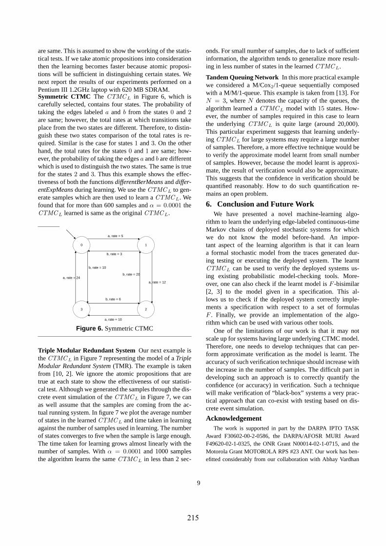
are same. This is assumed to show the working of the statis-tical tests. If we take atomic propositions into considerationthen the learning becomes faster because atomic proposi-tions will be sufficient in distinguishing certain states. Wenext report the results of our experiments performed on aPentium III 1.2GHz laptop with 620 MB SDRAM.Symmetric CTMC The CTMCL in Figure 6, which iscarefully selected, contains four states. The probability oftaking the edges labeleda and b from the states0 and 2are same; however, the total rates at which transitions takeplace from the two states are different. Therefore, to distin-guish these two states comparison of the total rates is re-quired. Similar is the case for states1 and3. On the otherhand, the total rates for the states0 and1 are same; how-ever, the probability of taking the edgesa andb are differentwhich is used to distinguish the two states. The same is truefor the states2 and3. Thus this example shows the effec-tiveness of both the functionsdifferentBerMeansanddiffer-entExpMeansduring learning. We use theCTMCL to gen-erate samples which are then used to learn aCTMCL. Wefound that for more than 600 samples andα = 0.0001 theCTMCL learned is same as the originalCTMCL.

0

3 2

1

a, rate = 5

b, rate = 3

b, rate = 10

b, rate = 20 a, rate = 24

a, rate = 12

b, rate = 6

a, rate = 10

Figure 6. Symmetric CTMC

Triple Modular Redundant System Our next example istheCTMCL in Figure 7 representing the model of aTripleModular Redundant System(TMR). The example is takenfrom [10, 2]. We ignore the atomic propositions that aretrue at each state to show the effectiveness of our statisti-cal test. Although we generated the samples through the dis-crete event simulation of theCTMCL in Figure 7, we canas well assume that the samples are coming from the ac-tual running system. In figure 7 we plot the average numberof states in the learnedCTMCL and time taken in learningagainst the number of samples used in learning. The numberof states converges to five when the sample is large enough.The time taken for learning grows almost linearly with thenumber of samples. Withα = 0.0001 and 1000 samplesthe algorithm learns the sameCTMCL in less than 2 sec-

onds. For small number of samples, due to lack of sufficientinformation, the algorithm tends to generalize more result-ing in less number of states in the learnedCTMCL.

Tandem Queuing Network In this more practical examplewe considered a M/Cox2/1-queue sequentially composedwith a M/M/1-queue. This example is taken from [13]. ForN = 3, whereN denotes the capacity of the queues, thealgorithm learned aCTMCL model with15 states. How-ever, the number of samples required in this case to learnthe underlyingCTMCL is quite large (around 20,000).This particular experiment suggests that learning underly-ing CTMCL for large systems may require a large numberof samples. Therefore, a more effective technique would beto verify the approximate model learnt from small numberof samples. However, because the model learnt is approxi-mate, the result of verification would also be approximate.This suggests that the confidence in verification should bequantified reasonably. How to do such quantification re-mains an open problem.

6. Conclusion and Future WorkWe have presented a novel machine-learning algo-

rithm to learn the underlying edge-labeled continuous-timeMarkov chains of deployed stochastic systems for whichwe do not know the model before-hand. An impor-tant aspect of the learning algorithm is that it can learna formal stochastic model from the traces generated dur-ing testing or executing the deployed system. The learntCTMCL can be used to verify the deployed systems us-ing existing probabilistic model-checking tools. More-over, one can also check if the learnt model isF -bisimilar[2, 3] to the model given in a specification. This al-lows us to check if the deployed system correctly imple-ments a specification with respect to a set of formulasF . Finally, we provide an implementation of the algo-rithm which can be used with various other tools.

One of the limitations of our work is that it may notscale up for systems having large underlying CTMC model.Therefore, one needs to develop techniques that can per-form approximate verification as the model is learnt. Theaccuracy of such verification technique should increase withthe increase in the number of samples. The difficult part indeveloping such an approach is to correctly quantify theconfidence (or accuracy) in verification. Such a techniquewill make verification of “black-box” systems a very prac-tical approach that can co-exist with testing based on dis-crete event simulation.

AcknowledgementThe work is supported in part by the DARPA IPTO TASK

Award F30602-00-2-0586, the DARPA/AFOSR MURI AwardF49620-02-1-0325, the ONR Grant N00014-02-1-0715, and theMotorola Grant MOTOROLA RPS #23 ANT. Our work has ben-efitted considerably from our collaboration with Abhay Vardhan

9

215

3

0

4

1

2

a, rate=3λ

a, rate=λ

a, rate=2λ

b, rate=µ

b, rate=µ

b, rate=µ

c, rate=νc, rate=ν

c, rate=νc, rate=ν

a, rate=δ

0

0.5

1

1.5

2

100 200 300 400 500 600 700 800 900 1000

Tim

e

Number of Samples

0

1

2

3

4

5

6

0 200 400 600 800 1000

Num

ber

of S

tate

s

Number of Samples

Figure 7. Learning TMR

on “learning to verify” framework for verifying infinite state sys-tems. We would like to thank Tom Brown for giving us feedbackon a previous version of this paper.

References

[1] D. Angluin. Learning regular sets from queries and coun-terexamples.Infor. and Comp., 75(2):87–106, 1987.

[2] C. Baier, B. Haverkort, H. Hermanns, and J. Katoen. Modelchecking continuous-time Markov chains by transient analy-sis. InComputer Aided Verification (CAV’00), volume 1855of LNCS, pages 358–372. Springer, 2000.

[3] C. Baier, J. Katoen, H. Hermanns, and B. Haverkort. Simu-lation for continuous-time Markov chains. In13th Interna-tional Conference on Concurrency Theory (CONCUR’02),volume 2421 ofLNCS, pages 338–354. Springer, 2002.

[4] G. Balbo, G. Conte, S. Donatelli, G. Franceschinis, andM. A. Marsan.Modelling with Generalized Stochastic PetriNets. John Wiley & Sons, 1995.

[5] L. Baum, T. Petrie, G. Soules, and N. Weiss. A maximiza-tion technique occuring in the statistical analysis of proba-bilistic functions of Markov chains.Annals of MathematicalStatistics, 41(1):164–171, 1970.

[6] R. C. Carrasco and J. Oncina. Learning stochastic regulargrammars by means of a state merging method. InInterna-tional Colloquium Grammatical Inference and Applications(ICGI’94), volume 862 ofLNCS. Springer, 1994.

[7] J. M. Cobleigh, D. Giannakopoulou, and C. S. Pasareanu.Learning assumptions for compositional verification. InTools and Algorithms for the Construction and Analysis ofSystems (TACAS’03), volume 2619 ofLNCS, pages 331–346.

[8] E. M. Gold. Language identification in the limit.Informa-tion and Control, 10:447–474, 1967.

[9] A. Groce, D. Peled, and M. Yannakakis. Adaptive modelchecking. InTools and Algorithms for the Constructionand Analysis of Systems (TACAS’02), volume 2280 ofLNCS,pages 357–371, 2002.

[10] B. Haverkort. Performance of Computer CommunicationSystems: A Model-Based Approach. Wiley, 1998.

[11] H. Hermanns, U. Herzog, and J. Katoen. Process algebrafor performance evaluation.Theoretical Computer Science,274(1–2):43–87, 2002.

[12] H. Hermanns, J. P. Katoen, J. Meyer-Kayser, and M. Siegle.A tool for model-checking Markov chains.Software Toolsfor Technology Transfer, 4(2):153–172, 2003.

[13] H. Hermanns, J. Meyer-Kayser, and M. Siegle. Multi-terminal binary decision diagrams to represent and analysecontinuous-time Markov chains. InWorkshop on the Numer-ical Solution of Markov Chains (NSMC’99), 1999.

[14] J. Hillston.A Compositional Approach to Performance Mod-elling. Cambridge University Press, 1996.

[15] R. V. Hogg and A. T. Craig.Introduction to MathematicalStatistics. Macmillan, New York, NY, USA, 1978.

[16] C. Kermorvant and P. Dupont. Stochastic grammatical infer-ence with multinomial tests. InGrammatical Inference: Al-gorithms and Applications, volume 2484 ofLecture Notes inArtificial Intelligence. Springer, 2002.

[17] M. Z. Kwiatkowska, G. Norman, and D. Parker. PRISM:Probabilistic symbolic model checker. InComputer Per-formance Evaluation, Modelling Techniques and Tools(TOOLS’02), volume 2324 ofLNCS, pages 200–204.

[18] W. Nelson.Applied Life Data Analysis. Wiley, 1982.[19] J. Oncina and P. Garcia. Inferring regular languages in poly-

nomial update time. InPattern Recognition and Image Anal-ysis, volume 1 ofSeries in Machine Perception and ArtificialIntelligence, pages 49–61. 1992.

[20] D. Ron, Y. Singer, and N. Tishby. On the learnability and us-age of acyclic probabilistic finite automata.Journal of Com-puter and System Sciences, 56(2):133–152, 1998.

[21] K. Sen, M. Viswanathan, and G. Agha. Statistical modelchecking of black-box probabilistic systems. In16th confer-ence on Computer Aided Verification (CAV’04), LNCS (ToAppear). Springer, July 2004.

[22] W. J. Stewart. Introduction to the Numerical Solution ofMarkov Chains. Princeton, 1994.

[23] W. Wei, B. Wang, and D. Towsley. Continuous-time hiddenMarkov models for network performance evaluation.Perfor-mance Evaluation, 49(1–4):129–146, September 2002.

[24] H. L. S. Younes, M. Kwiatkowska, G. Norman, andD. Parker. Numerical vs. statistical probabilistic modelchecking: An empirical study. InTools and Algorithms forthe Construction and Analysis of Systems (TACAS’04), vol-ume 2988 ofLNCS. Springer, 2004.

10

216

Towards a Hierarchical Taxonomy of AutonomousAgents∗

Predrag T. Tosic and Gul A. AghaOpen Systems Laboratory, Department of Computer Science

University of Illinois at Urbana-Champaign, USAE-mail: p-tosic, agha@cs.uiuc.edu

Abstract – Autonomous agents have become an influentialand powerful paradigm in a great variety of disciplines,from sociology and economics to distributed artificial in-telligence and software engineering to philosophy. Giventhat the paradigm has been around for awhile, one wouldexpect a broadly agreed-upon, solid understanding of whatautonomous agents are and what they are not. This, how-ever, is not the case. We therefore join the ongoing debateon what are the appropriate notions of autonomous agency.We approach agents and agent ontology from a cybernet-ics and general systems perspective, in contrast to the muchmore common in the agent literature sociology, anthropologyand/or cognitive psychology based approaches. We attemptto identify the most fundamental attributes of autonomousagents, and propose a tentative hierarchy of autonomousagents based on those attributes.

Keywords: Smart Agents, Intelligent Systems, Intelligentand Soft Computing - Systems and Applications

1 Introduction and MotivationAutonomous agents have become a powerful paradigm in

a great variety of disciplines, from sociology and economicsto distributed artificial intelligence and software engineeringto cognitive sciences to philosophy. While different disci-plines have different needs and may have different notionsof agents, the agents in economics and those in distributedartificial intelligence (DAI), for example, nonetheless tendto share most of the fundamental properties. Given that theparadigm has been around for awhile, one would expect a rel-atively solid understanding of what autonomous agents are,and what they are not. This, however, is not at all the case.

Is there, then, at least a reasonably unified and broadlyagreed upon notion ofautonomous agencyamong the com-puter scientists? The answer is still‘No.’ In particular,the notion of autonomous agency in open distributed com-puting environments (e.g., [2, 6]), while certainly sharingsome of the properties, does not coincide with the corre-sponding standard notion of agency in artificial intelligence(e.g., [18]). One would hope that understanding this gap

∗0-7803-8566-7/04/$20.00c© 2004 IEEE.

can assist in bridging it, thereby enhancing the ability of thesoftware system designers to meet the requirements of vari-ous AI and other applications more effectively and easily byreadily identifying and efficiently building the required ad-ditional functionality (“agent capabilities”) on the top of theexisting open distributed agent-based (or even merely object-based) software infrastructures.

Herewith, we attempt to contribute to the ongoing debateon what are the appropriate notions ofautonomous agency.Instead of proposing a single such prescriptive (and there-fore necessarily also restrictive), “one size fits all” defini-tion of autonomous agents, we propose an entire hierarchyof agents, from simpler (reactive situated agents) towardsquite complicated and capable of human-like complex cog-nitive tasks (deliberative, intelligent agents). The proposedhierarchy, rather than being based on any particular schoolof thought in artificial intelligence and cognitive sciences, ischiefly based on ideas and paradigms from other scientificdisciplines - mainlycybernetics [25] and systems science[14, 15]. We argue that learning from other, non-AI and non-cognitive disciplines such as cybernetics or biology can pro-vide some critical, yet thus far for the most part missing,ingredients in building successful and complete theories ofartificial autonomous agents and multi-agent systems. Thiswork is intended to be a modest step in that direction.

2 What Are Autonomous Agents?It has become common to define an appropriate notion of

agency by specifying thenecessary attributesthat all agentsof the particular kind one has in mind are required to share(e.g., [10, 16, 18]). There has been much of debate, however,what set of properties exactly qualifies an entity, such as asingle human decision maker, a firm in the market, a com-puter program, a robot or an unmanned autonomous vehicle,for an autonomousor an intelligent agent. Influential po-sition papers, such as [26] for intelligent agents or [10] forautonomous agents, while trying to clarify and unify the ter-minology, and propose agent taxonomies, also illustrate theheterogeneity and lack of agreement on the definition andthe required (as opposed to optional) properties even in thecase of autonomous agents that are restricted to computer

217

programs alone (which disallows, say, humans or social in-sects).

It has been observed that the main division line is the onethat separates the (purely)reactive agents[17, 18] from themore complex, capable of cognitive-like behaviorsdeliber-ative agents [16, 18, 26]. A reactive agent is one that iscoupled to the environment and is capable of being affectedby, and perhaps in turn also affecting, the environment. Itneed not be capable of cognitive tasks such as learning, plan-ning or reasoning. It need not have any complicated internalstructure, or any capability of complex correlations betweenits internal states and the states of the outer world (“symbolicrepresentations”); it uses a little or no memory, etc.

In contrast, a deliberative agent is much more complex interms of its internal structure, is typically capable of creat-ing and working with abstract representations of a complexouter world (e.g., by performing planning, reasoning and/orlearning tasks), has some sense of its purpose (tasks, goals,utilities), usually is pro-active and adaptable, etc. Much ofresearch in the main-stream artificial intelligence (AI) overthe past twenty or more years has been focused on the de-sign problem of such artificial deliberative agents, capableof acting in complex environments and autonomously pursu-ing their complex goals or tasks in such environments (see,e.g., [6, 16, 18, 24, 26] and references therein).

Herein, we attempt to hierarchically classify agents basedon their complexity in terms of their capabilities and func-tionalities, not on (models of) agents’ internal structure. Anagent is more sophisticated than another, if it is capable ofmore complex behaviors observable by an outside observer.This natural functionalist, behaviorist and systems theoryoriented approach, however, does not seem very common inthe mainstream agent literature.

Some of the most frequently encountered general prop-erties of agents found in the literature include reactive-ness, pro-activeness, ability to execute autonomously, goal-orientedness or goal-drivenness, a capability of sensing theenvironment and being affected by the environment, a ca-pability of affecting the environment, sociability, ability tocommunicate, persistence, purposefulness, and ability tolearn and/or reason about the world.

Not all the agents have to possess all of the above men-tioned properties, of course. We shall make an attempt, how-ever, to identify those properties that arenecessaryfor au-tonomous agents of a desired level of complexity.

In case of the computer programs, being capable of au-tonomous execution, that is, an execution that is not (en-tirely) controlled from the outside, seems to be the most natu-ral requirement for any notion of autonomous agency. How-ever, a question then arises, is this enough? For instance, afinite state machine (FSM)executes autonomously (and re-actively, inasmuch as the ability of an agent to be affected bythe environment suffices for reactivity), but we find it hardto considerindividual FSMs an appropriate abstraction ofautonomous agents. On the other hand, acoupled finite au-tomata model has been proposed as an abstraction of reac-

tive situated agents (e.g., [17]). We shall discuss in somedetail what we consider to be the necessary attributes of au-tonomous agency, as well as propose a hierarchy of agents interms of the attributes they possess, inSection 4.

3 A Systems Approach To AgentsMost approaches to classifying various types of (natural

as well as artificial) agents are based on specifying the nec-essary attributes of a particular kind of agents, as in, e.g.,[10]. We adopt this general approach, as well. However, wealso try to be more specific as towhat kinds of attributeswe allow. Tools from other cognitive disciplines, such aspsychology, anthropology and sociology, have been liber-ally applied to characterize the fundamental properties, andtherefore the very nature, of various artificial agent systems.In particular, software and robotic agents have been gener-ously ascribed properties that characterize anthropomorphiccognition, such as beliefs, desires, intentions, emotions, etc.One of the most successful examples of such approach arethe BDI agent paradigm and architectures [16].

However, we see some potential conceptual and practicalproblems with assigning too liberally human (cognitive orother) attributes to a piece of software or a robot. In scien-tific and engineering modeling, the very purpose of amodelis to be intrinsically simpler, and therefore more amenable toanalysis, than the phenomenon being modeled. But when theattributes of beliefs, intentions, emotions, and the like are as-cribed to, for instance, a software agent system with individ-ual agents of a fairly modest complexity, it seems that exactlythe opposite is the case. While there is some justification incorrelating, for instance, how artificial agents represent andinteract with complex, partially observable environments andtasks to how humans act (reason, learn, represent knowledge,etc.) with respect to their tasks and environments, there arealso certain dangers in this approach. For, after all, robotsand software agents are not human, and (unless one believesin the Strong AI hypothesis [19]) perhaps cannot ever bemade very human-like in terms of their cognitive capabil-ities. Furthermore, representing and reasoning about rela-tively simple software agents encountered in many softwareengineering applications in terms of highly complex capa-bilities of human-like cognition seems to be an “overkill”, inthat the complexity of the model may end up considerablyexceeding the sophistication of the modeled.

Another problem with attributing various anthropomor-phic features to artificial agents emerges once different typesof such agents are compared and contrasted with one an-other. Software agents, robots and other types of artificialagents are man-designed engineering systems. They shouldbe characterized, studied, compared and contrasted to oneanother in terms of how they as systemsbehave, not what“mental states” or “beliefs” or “desires” or “emotions” theirdesigner attributes to them. Whether an agent is reactive oradaptable can be, in general, verified by an outside observerthat is independent of the agent. What are the belief or desireor emotional states of an agent, on the other hand, cannot.

218

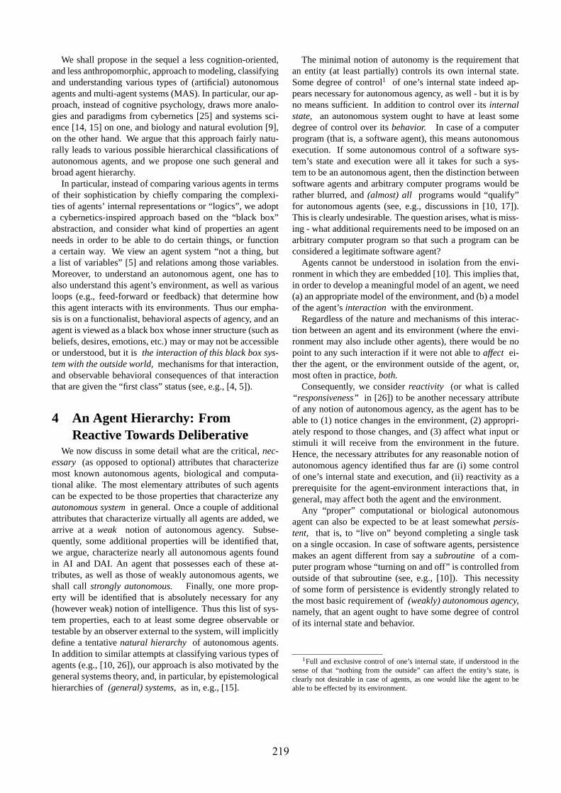
We shall propose in the sequel a less cognition-oriented,and less anthropomorphic, approach to modeling, classifyingand understanding various types of (artificial) autonomousagents and multi-agent systems (MAS). In particular, our ap-proach, instead of cognitive psychology, draws more analo-gies and paradigms from cybernetics [25] and systems sci-ence [14, 15] on one, and biology and natural evolution [9],on the other hand. We argue that this approach fairly natu-rally leads to various possible hierarchical classifications ofautonomous agents, and we propose one such general andbroad agent hierarchy.

In particular, instead of comparing various agents in termsof their sophistication by chiefly comparing the complexi-ties of agents’ internal representations or “logics”, we adopta cybernetics-inspired approach based on the “black box”abstraction, and consider what kind of properties an agentneeds in order to be able to do certain things, or functiona certain way. We view an agent system “not a thing, buta list of variables” [5] and relations among those variables.Moreover, to understand an autonomous agent, one has toalso understand this agent’s environment, as well as variousloops (e.g., feed-forward or feedback) that determine howthis agent interacts with its environments. Thus our empha-sis is on a functionalist, behavioral aspects of agency, and anagent is viewed as a black box whose inner structure (such asbeliefs, desires, emotions, etc.) may or may not be accessibleor understood, but it isthe interaction of this black box sys-tem with the outside world,mechanisms for that interaction,and observable behavioral consequences of that interactionthat are given the “first class” status (see, e.g., [4, 5]).

4 An Agent Hierarchy: FromReactive Towards Deliberative

We now discuss in some detail what are the critical,nec-essary (as opposed to optional) attributes that characterizemost known autonomous agents, biological and computa-tional alike. The most elementary attributes of such agentscan be expected to be those properties that characterize anyautonomous systemin general. Once a couple of additionalattributes that characterize virtually all agents are added, wearrive at aweak notion of autonomous agency. Subse-quently, some additional properties will be identified that,we argue, characterize nearly all autonomous agents foundin AI and DAI. An agent that possesses each of these at-tributes, as well as those of weakly autonomous agents, weshall call strongly autonomous. Finally, one more prop-erty will be identified that is absolutely necessary for any(however weak) notion of intelligence. Thus this list of sys-tem properties, each to at least some degree observable ortestable by an observer external to the system, will implicitlydefine a tentativenatural hierarchy of autonomous agents.In addition to similar attempts at classifying various types ofagents (e.g., [10, 26]), our approach is also motivated by thegeneral systems theory, and, in particular, by epistemologicalhierarchies of(general) systems,as in, e.g., [15].

The minimal notion of autonomy is the requirement thatan entity (at least partially) controls its own internal state.Some degree of control1 of one’s internal state indeed ap-pears necessary for autonomous agency, as well - but it is byno means sufficient. In addition to control over itsinternalstate, an autonomous system ought to have at least somedegree of control over itsbehavior. In case of a computerprogram (that is, a software agent), this means autonomousexecution. If some autonomous control of a software sys-tem’s state and execution were all it takes for such a sys-tem to be an autonomous agent, then the distinction betweensoftware agents and arbitrary computer programs would berather blurred, and(almost) all programs would “qualify”for autonomous agents (see, e.g., discussions in [10, 17]).This is clearly undesirable. The question arises, what is miss-ing - what additional requirements need to be imposed on anarbitrary computer program so that such a program can beconsidered a legitimate software agent?

Agents cannot be understood in isolation from the envi-ronment in which they are embedded [10]. This implies that,in order to develop a meaningful model of an agent, we need(a) an appropriate model of the environment, and (b) a modelof the agent’sinteraction with the environment.

Regardless of the nature and mechanisms of this interac-tion between an agent and its environment (where the envi-ronment may also include other agents), there would be nopoint to any such interaction if it were not able toaffect ei-ther the agent, or the environment outside of the agent, or,most often in practice,both.

Consequently, we considerreactivity (or what is called“responsiveness” in [26]) to be another necessary attributeof any notion of autonomous agency, as the agent has to beable to (1) notice changes in the environment, (2) appropri-ately respond to those changes, and (3) affect what input orstimuli it will receive from the environment in the future.Hence, the necessary attributes for any reasonable notion ofautonomous agency identified thus far are (i) some controlof one’s internal state and execution, and (ii) reactivity as aprerequisite for the agent-environment interactions that, ingeneral, may affect both the agent and the environment.

Any “proper” computational or biological autonomousagent can also be expected to be at least somewhatpersis-tent, that is, to “live on” beyond completing a single taskon a single occasion. In case of software agents, persistencemakes an agent different from say asubroutine of a com-puter program whose “turning on and off” is controlled fromoutside of that subroutine (see, e.g., [10]). This necessityof some form of persistence is evidently strongly related tothe most basic requirement of(weakly) autonomous agency,namely, that an agent ought to have some degree of controlof its internal state and behavior.

1Full and exclusive control of one’s internal state, if understood in thesense of that “nothing from the outside” can affect the entity’s state, isclearly not desirable in case of agents, as one would like the agent to beable to be effected by its environment.

219

We summarize below our notion ofweakly autonomousagency (WAA)2 in terms of the necessary agent attributes:

weak autonomous agency≈ control of own state+ reactivity + persistence

Hence, at the bottom level of the emerging hierarchy ofautonomous agents, we find purely reactive embedded (orsituated) agents [17]. Such agents can be appropriately ab-stracted via finite state machines (deterministic case) or dis-crete Markov chains (probabilistic case). A combinationof reactivity and persistence characterizes many of both thesimplest life forms and simple artificial agents. When somedegree of control of the agent’s internal state and behavioris also present, one arrives at what we shall call herewithweakly autonomous agency (WAA).We suggest the actormodel of distributed computing [1, 2] to be a canonical ex-ample ofWAA among the software agents.

One common feature found in all or nearly all interestingautonomous agents, biological and computational alike, issome form of goal-orientednessor goal-drivenness. Incase of the living organisms, the highest level driving mech-anisms are the instincts ofsurvival and reproduction. Thesingle most fundamental instinct in all of known life forms(to which an appropriate notion of an instinct can be ascribedat all) is that of survival. Indeed, the instinct of reproductionis related to the survival of the species or, perhaps, of theparticular genes and gene patterns, as opposed to the “mere”survival of the individual organisms [9]. At lower levels, thedriving mechanisms - finding food or a sexual partner - arethose that are expected to provide, promote and enhance thetwo highest-level goals, survival and reproduction.

In the case of artificial computational agents such as a webcrawler or a robot or an autonomous unmanned vehicle, theseagents are designed and programmed with a particular goalor a set of goals in designer’s mind. Thus, the ability to actautonomously is typically related to an agent having somegoal(s) to accomplish, and therefore being goal-driven.

From a systems perspective, in order for an agent to bereactive, it has to becoupled to its environment via someappropriate sensors (or “input channels”) and effectors (“out-put channels”). Due to agent’s sensors, the environment canaffect the agent; due to agent’s effectors, the agent can affectthe outside environment. For a stronger notion of agencythanWAA, in addition to some sort of sensors and effectors,necessary to ensure that the agent can interact with, affectand be affected by the outside world, it seems natural thatan appropriate feedback, or control, loop exists between theagent and the outside world, so that this feedback loop af-fects how the agent responds to the environmental changes.A feedback loop provides the agent with knowledge of “howwell it is doing”. In particular, an agent will have use of afeedback loop only if it has an appropriate notion of its goalsor tasks, and an evaluation function (task value, utility, re-

2This notion of weak agent autonomy, mainly based on the dominant no-tion of autonomous agents in the area of software design for open distributedsystems, is obviously not calledweak by those who consider it sufficient fortheir purposes.

source consumption, or the like) associated with it. That is,an agent needs some sort of acontrol loop in order to becapable of goal-oriented or utility-oriented behavior.

Finally, in addition to responsiveness, persistence andgoal-drivenness or goal-orientedness, one more characteris-tic found in nearly all interesting autonomous agents, notaltogether unrelated to goal-orientedness, is that ofpro-activeness [10, 18, 26]. While some literature on au-tonomous agents treats pro-activeness and goal-drivennessas synonyms, we briefly discuss why, in general, the two at-tributes ought to be distinguished.

Namely, a situated, reactive agent can be goal-orientedwithout being pro-active: given an input from the “world”,the goal-oriented agent acts so as to ensure, e.g., avoidingbeing in certain of its internal states that it views incom-patible with its limited knowledge of “what is going on outthere”. If there are no changes in the environment, the agentsimply keeps “sitting” in whatever its current state happensto be. Thus, this reactive agent has a goal (although admit-tedly a very simplistic one), but is not pro-active. Similarly,an agent can be pro-active without being goal-oriented, aslong as we require of agent’s goal(s) to be non-trivial, and,in particular, to possibly entail some deliberate effect that theagent’s actions may be required, under appropriate circum-stances, to have on the environment. Under this assumption,an agent may “pro-actively” perform a more or less randomwalk among its internal states, without any observable effectson the outside world, and therefore without accomplishing -or, indeed, having - any specific goals insofar as the agent’sdeliberate influence on the environment.

Thus, while pro-activeness and goal-orientedness are usu-ally closely related, they are not synonymous, and, moreover,neither subsumes the other.

Once aWAA agent is additionally equipped with someform of goal-drivenness and pro-activeness, we arrive atwhat we define asstrongly autonomous agency (SAA).Mostagents encountered in AI, whether they are software agents,robots, unmanned vehicles, or of any other kind, are of this,strongly autonomous type (see, e.g., [18, 16, 24]).

Therefore, we find that it is precisely the properties of (i)some degree of control of one’s own internal state and behav-ior, (ii) reactiveness or responsiveness, (iii) persistence, (iv)pro-activeness, and (v) goal-drivenness or goal-orientednessthat, together, and in synergy with each other, make an agenttruly (or strongly) autonomousin an AI sense:

strong autonomous agency≈ weak autonomous agency+ goal-orientedness + pro-activeness

Granted, much of the agent literature has identified prop-erties (i) - (v) as common to autonomous agents (see, e.g.,[26, 10] and references therein). We claim, however, thatthese five agent capabilities arethe necessary proper-ties that are all found in nearly every reasonable model ofautonomous agency, whereas other characteristics, includ-ing sociability, mobility, “mental states”, beliefs-desires-intentions, etc., are not as essential, and are found in (or canbe reasonably attributed to) onlysome, but by no means

220

(nearly) all of the known autonomous agents, whether bio-logical or artificial.

However, even those living organisms that one wouldnever consider intelligent have one more fundamental prop-erty, absent from our notion ofSAA, and that is the abil-ity to adapt (e.g., through metabolism). Adaptability is anecessary prerequisite for biological survival, as well as forany reasonable notion of intelligence. The “control loop” be-tween the agent and the world serves no purpose, if the agenthas no goals or notions of “goodness” with respect to whichit tries to optimize its behavior. But such goal- or utility-drivenness is useless, if the agent cannot dynamically adjustits behavior based on the feedback, i.e., if it cannot adapt.

To summarize, based on how is an agent coupled to its en-vironment, how complex properties of that environment theparticular type of coupling (e.g., type of sensors, “controlloop”, effectors) can capture, and how complex behaviors oractions the agent is capable of, we have proposed a tenta-tive general hierarchical classification of autonomous agentsembedded in, and acting as a part of, their environments.

Whether one would consider an agent that (i) has at leastsome control over its internal state and behavior, and is (ii)reactive, (iii) persistent, (iv) pro-active, (v) goal- or utility-driven, and (vi) adaptable, to automatically beintelligent,depends on one’s definition of intelligence and is subject todebate. What seems clear, however, is that no proper subsetof the properties (i) - (vi) satisfies even the weakest notion ofintelligence. Moreover, we argue that, as one keeps addingon properties from (i) towards (vi), one can recognize manywell-known examples of agents found in the literature, yetnot as a part of what we argue is a reasonable and naturalhierarchy of agents3. For instance, artificial agents that pos-sess only (i), (ii) and possibly (iii) are studied in detail in[17]. Some examples ofWAA agents possessing (i) - (iii)andSAA agents having attributes (i) - (v) are discussed next.

5 Discussion and Some ApplicationsTo illustrate the usefulness of the proposed hierarchy

of agents, we consider some software engineering de-velopments in the context of open distributed systems.Agent-oriented programming [20] can be viewed both as anovel paradigm and the natural successor to object-orientedparadigm [13]. The transition from object-oriented towardsagent-oriented programming was motivated by the design ofopen distributed platforms, so that concurrency and resourcesharing can be exploited in heterogeneous distributed envi-ronments [3].

To place the development of a general paradigm of au-tonomous agency into a broader computer science perspec-tive, we briefly make a comparison to the development ofthe object-oriented paradigm. The primary motivation formoving away from function evaluation based classical im-perative programming towards the object-oriented program-ming paradigm was primarily motivated by the nature of a

3However, see [10] for another proposal of a hierarchical taxonomy ofvarious types of agents.

great number of emerging applications, where it was morenatural to think in terms of objects and their classes and hi-erarchies, their capabilities (“methods”), etc., then in termsof functions being evaluated on variables. One particular do-main that gave a huge impetus to the growth and successof object-oriented programming was that of computer simu-lation of various complex and distributed infrastructures [8].As computing started becoming increasingly distributed bothphysically and logically, and these distributed systems get-ting increasingly heterogeneous, complex and open, the in-dividual components, whether hardware or software, weremoving away from non-autonomous components of a single,tightly coupled system, towards being increasingly sophis-ticated, autonomous and complex (sub)systems themselves,that were only loosely coupled into an overarching largersystem. Hence, a novel paradigm capturing the increasingrequirements in terms of autonomy, flexibility and complex-ity of the individual components in such distributed systemswas sought - and, in case of the software, theagent-basedprogrammingparadigm was born [20].

We thus see the relationship of agent-oriented program-ming to object-oriented programming, in essence, similarto the relationship of object-oriented to classical imperativeprogramming: each is a novel metaphor and a radical depar-ture from its predecessor - yet a novel metaphor that clearlybuilds on the top of its predecessor, and adds more desir-able properties that brings thus enhanced model considerablycloser to the target applications.

Actors [1, 2] are a powerful model for specifying coordi-nation in open distributed systems. In addition to its internalstate, an actor also encapsulates its behavior (both data andprocedure). An actor can communicate via asynchronousmessage passing with other actors; this asynchronous com-munication is, therefore, central to how actors interact withtheir environment. An actor is responsive or reactive; it alsomay (but need not) be persistent. Actors thus fit well into ourconcept ofweakly autonomous agency.

Actors can also be used as a building block towards imple-menting more complex systems and, in particular, for soft-ware design of autonomous agents with stronger autonomouscapabilities, via appropriate extensions (added functionality)of the basic actor model. For instance, ref. [3] addressesan important problem of how to extend actors into a pow-erful concurrent programming paradigm fordistributed ar-tificial intelligence (DAI) [6, 24]. There are other exam-ples of designing strongly autonomous applications on thetop of weakly autonomous infrastructures. For instance, anactor-based (hence, “weakly autonomous”) software infras-tructure is used in [11, 12] to build a simulator of a particu-lar kind of strongly autonomous agents, namely, autonomousunmanned vehicles [22, 23]. The basic agent capabilitiesare provided by the actor infrastructure, whereas the higher-order autonomous abilities, such as the pro-active pursuit ofan agent’s goals or the agents’ coordination strategies, arebuilt on the top of the basic actor architecture, i.e., at the“application software” level [11, 22, 23].

221

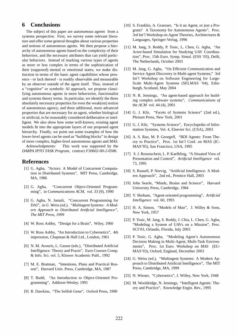
6 ConclusionsThe subject of this paper areautonomous agentsfrom a

systems perspective. First, we survey some relevant litera-ture and offer some general thoughts about various propertiesand notions of autonomous agents. We then propose a hier-archy of autonomous agents based on the complexity of theirbehaviors, and the necessary attributes that can yield partic-ular behaviors. Instead of marking various types of agentsas more or less complex in terms of the sophistication oftheir (supposed) mental or emotional states, we make dis-tinction in terms of the basic agent capabilities whose pres-ence - or lack thereof - is readily observable and measurableby an observer outside of the agent itself. Thus, instead ofa “cognitive” or symbolic AI approach, we propose classi-fying autonomous agents in more behaviorist, functionalistand systems theory terms. In particular, we identify the threeabsolutely necessary properties for even the weak(est) notionof autonomous agency, and three additional, more advancedproperties that are necessary for an agent, whether biologicalor artificial, to be reasonably considered deliberative or intel-ligent. We also show how some well-known, existing agentmodels fit into the appropriate layers of our proposed agenthierarchy. Finally, we point out some examples of how thelower-level agents can be used as “building blocks” in designof more complex, higher-level autonomous agents andMAS.

Acknowledgments: This work was supported by theDARPA IPTO TASK Program, contractF30602-00-2-0586.

References[1] G. Agha, “Actors: A Model of Concurrent Computa-

tion in Distributed Systems”, MIT Press, Cambridge,MA, 1986

[2] G. Agha, “Concurrent Object-Oriented Program-ming”, in Communications ACM,vol. 33 (9), 1990

[3] G. Agha, N. Jamali, “Concurrent Programming forDAI”, in G. Weiss (ed.), “Multiagent Systems: A Mod-ern Approach to Distributed Artificial Intelligence”,The MIT Press, 1999

[4] W. Ross Ashby, “Design for a Brain”, Wiley, 1960

[5] W. Ross Ashby, “An Introduction to Cybernetics”, 4thimpression, Chapman & Hall Ltd., London, 1961

[6] N. M. Avouris, L. Gasser (eds.), “Distributed ArtificialIntelligence: Theory and Praxis”, Euro Courses Comp.& Info. Sci. vol. 5, Kluwer Academic Publ., 1992

[7] M. E. Bratman, “Intentions, Plans and Practical Rea-son”, Harvard Univ. Press, Cambridge, MA, 1987

[8] T. Budd, “An Introduction to Object-Oriented Pro-gramming”, Addison-Wesley, 1991

[9] R. Dawkins, “The Selfish Gene”, Oxford Press, 1990

[10] S. Franklin, A. Graesser, “Is it an Agent, or just a Pro-gram? A Taxonomy for Autonomous Agents”, Proc.3rd Int’l Workshop on Agent Theories, Architectures &Languages, Springer-Verlag, 1996

[11] M. Jang, S. Reddy, P. Tosic, L. Chen, G. Agha, “AnActor-based Simulation for Studying UAV Coordina-tion”, Proc. 15th Euro. Symp. Simul. (ESS ’03), Delft,The Netherlands, October 2003

[12] M. Jang, G. Agha, ”On Efficient Communication andService Agent Discovery in Multi-agent Systems,” 3rdInt’l Workshop on Software Engineering for Large-Scale Multi-Agent Systems (SELMAS ’04), Edin-burgh, Scotland, May 2004

[13] N. R. Jennings, “An agent-based approach for build-ing complex software systems”,Communications ofthe ACM vol. 44 (4), 2001

[14] G. J. Klir, “Facets of Systems Science” (2nd ed.),Plenum Press, New York, 2001

[15] G. J. Klir, “Systems Science”, Encyclopedia of Infor-mation Systems, Vol. 4, Elsevier Sci. (USA), 2003

[16] A. S. Rao, M. P. Georgeff, “BDI Agents: From The-ory to Practice”, Proc. 1st Int’l Conf. on MAS (IC-MAS’95), San Francisco, USA, 1995

[17] S. J. Rosenschein, L. P. Kaelbling, “A Situated View ofPresentation and Control”,Artificial Intelligence vol.73, 1995

[18] S. Russell, P. Norvig, “Artificial Intelligence: A Mod-ern Approach”, 2nd ed., Prentice Hall, 2003

[19] John Searle, “Minds, Brains and Science”, HarvardUniversity Press, Cambridge, 1984

[20] Y. Shoham, “Agent-oriented programming”,ArtificialIntelligence vol. 60, 1993

[21] H. A. Simon, “Models of Man”, J. Willey & Sons,New York, 1957

[22] P. Tosic, M. Jang, S. Reddy, J. Chia, L. Chen, G. Agha,“Modeling a System of UAVs on a Mission”, Proc.SCI’03, Orlando, Florida, July 2003

[23] P. Tosic, G. Agha, “Modeling Agent’s AutonomousDecision Making in Multi-Agent, Multi-Task Environ-ments”, Proc. 1st Euro. Workshop onMAS (EU-MAS’03), Oxford, England, December 2003

[24] G. Weiss (ed.), “Multiagent Systems: A Modern Ap-proach to Distributed Artificial Intelligence”, The MITPress, Cambridge, MA, 1999

[25] N. Wiener, “Cybernetics”, J. Willey, New York, 1948

[26] M. Wooldridge, N. Jennings, “Intelligent Agents: The-ory and Practice”, Knowledge Engin. Rev., 1995

222

Characterizing Configuration Spaces of SimpleThreshold Cellular Automata

Predrag T. Tosic and Gul A. Agha

Open Systems Laboratory, Department of Computer ScienceUniversity of Illinois at Urbana-Champaign

Mailing address: Siebel Center for Computer Science,201 N. Goodwin Ave., Urbana, IL 61801, USA

p-tosic@cs.uiuc.edu, agha@cs.uiuc.edu

Abstract. We study herewith the simple threshold cellular automata (CA), asperhaps the simplest broad class of CA with non-additive (i.e., non-linear andnon-affine) local update rules. We characterize all possible computations of themost interesting rule for such CA, namely, the Majority (MAJ) rule, both inthe classical, parallel CA case, and in case of the corresponding sequential CAwhere the nodes update sequentially, one at a time. We compare and contrast theconfiguration spaces of arbitrary simple threshold automata in those two cases,and point out that some parallel threshold CA cannot be simulated by any oftheir sequential counterparts. We show that the temporal cycles exist only in caseof (some) parallel simple threshold CA, but can never take place in sequentialthreshold CA. We also show that most threshold CA have very few fixed pointconfigurations and few (if any) cycle configurations, and that, while the MAJsequential and parallel CA may have many fixed points, nonetheless “almost all”configurations, in both parallel and sequential cases, are transient states.

1 Introduction and Motivation

Cellular automata (CA) were originally introduced as an abstract mathematical modelof the behavior of biological systems capable of self-reproduction [15]. Subsequently,variants of CA have been extensively studied in a great variety of application domains,predominantly in the context of complex physical or biological systems and their dy-namics (e.g., [20, 21, 22]). However, CA can also be viewed as an abstraction of mas-sively parallel computers (e.g, [7]). Herein, we study a particular simple yet nontrivialclass of CA from a computer science perspective. This class are the threshold cellularautomata. In the context of such CA, we shall first compare and contrast the con-figuration spaces of the classical, concurrent CA and their sequential analogues. Wewill then pick a particular threshold node update rule, and fully characterize possiblecomputations in both parallel and sequential cases for the one-dimensional automata.

Cellular automata CA are an abstract computational model of fine-grain paral-lelism [7], in that the elementary operations executed at each node are rather simpleand hence comparable to the basic operations performed by the computer hardware. Ina classical, that is, concurrently executing CA, whether finite or infinite, all the nodesexecute their operations logically simultaneously: the state of a node at time step

223

is some simple function of the states (i) of the node itself, and (ii) of a set of

its pre-specified neighbors, at time.

We consider herewith the sequential version of CA, heretofore abridged to SCA,and compare such sequential CA with the classical, parallel (concurrent) CA. Inparticular, we show that there are 1-D CA with very simple node state update rules thatcannot be simulated by any comparable SCA, irrespective of the node update ordering.

We also fully characterize the possible computations of the most interesting case ofthreshold cellular automata, namely, the (S)CA with the Majority node update rule.

An important remark is that we use the terms parallel and concurrent as synonymsthroughout the paper. This is perhaps not the most standard convention, but we arenot alone in not making the distinction between the two terms (cf. discussion in [16]).Moreover, by a parallel (equivalently, concurrent) computation we shall mean actionsof several processing units that are carried out logically (if not necessarily physically)simultaneously. In particular, when referring to parallel or concurrent computation,we do assume a perfect synchrony.

2 Cellular Automata and Types of Their Configurations

We follow [7] and define classical (that is, synchronous and concurrent) CA in twosteps: by first defining the notion of a cellular space, and subsequently that of acellular automaton defined over an appropriate cellular space.

Definition 1: A Cellular Space, , is an ordered pair where isa regular graph (finite or infinite), with each node labeled with a distinct integer, and is a finite set of states that has at least two elements, one of which being the specialquiescent state, denoted by .

We denote the set of integer labels of the nodes (vertices) in by .

Definition 2: A Cellular Automaton (CA), A, is an ordered triple where is a cellular space, is a fundamental neighborhood, and is a finitestate machine such that the input alphabet of is , and the local transitionfunction (update rule) for each node is of the form ! "$#&%' for CA withmemory, and ()* +%, for memoryless CA.

Some of our results pertain to a comparison and contrast between the classical,concurrent threshold CA and their sequential counterparts, the threshold SCA.

Definition 3: A Sequential Cellular Automaton (SCA) S is an ordered quadruple-.0/1 , where -. and are as in Def. 2, and / is a sequence, finite or infinite,all of whose elements are drawn from the set of integers used in labeling the verticesof . The sequence / is specifying the sequential ordering according to which anSCA’s nodes update their states, one at a time.

However, when comparing and contrasting the concurrent threshold CA with theirsequential counterparts, rather than making a comparison between a given CA with aparticular SCA, we compare the parallel CA computations with the computations ofthe corresponding SCA for all possible sequences of node updates. To that end, thefollowing convenient terminology is introduced:

Definition 4: A Nondeterministic Interleavings Cellular Automaton (NICA) I isdefined to be the union of all sequential automata S whose first three components, -.

224

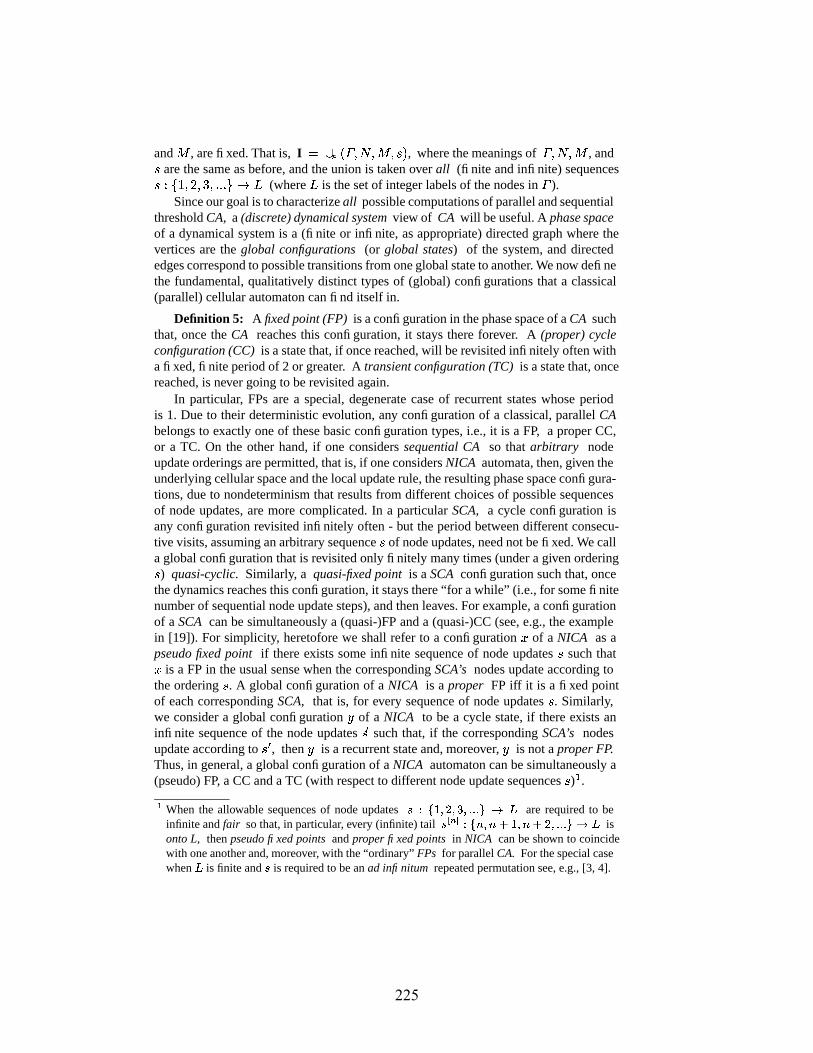
and , are fixed. That is, I -/1 , where the meanings of -. , and/ are the same as before, and the union is taken over all (finite and infinite) sequences/! ++ % (where is the set of integer labels of the nodes in ).

Since our goal is to characterize all possible computations of parallel and sequentialthreshold CA, a (discrete) dynamical system view of CA will be useful. A phase spaceof a dynamical system is a (finite or infinite, as appropriate) directed graph where thevertices are the global configurations (or global states) of the system, and directededges correspond to possible transitions from one global state to another. We now definethe fundamental, qualitatively distinct types of (global) configurations that a classical(parallel) cellular automaton can find itself in.

Definition 5: A fixed point (FP) is a configuration in the phase space of a CA suchthat, once the CA reaches this configuration, it stays there forever. A (proper) cycleconfiguration (CC) is a state that, if once reached, will be revisited infinitely often witha fixed, finite period of 2 or greater. A transient configuration (TC) is a state that, oncereached, is never going to be revisited again.

In particular, FPs are a special, degenerate case of recurrent states whose periodis 1. Due to their deterministic evolution, any configuration of a classical, parallel CAbelongs to exactly one of these basic configuration types, i.e., it is a FP, a proper CC,or a TC. On the other hand, if one considers sequential CA so that arbitrary nodeupdate orderings are permitted, that is, if one considers NICA automata, then, given theunderlying cellular space and the local update rule, the resulting phase space configura-tions, due to nondeterminism that results from different choices of possible sequencesof node updates, are more complicated. In a particular SCA, a cycle configuration isany configuration revisited infinitely often - but the period between different consecu-tive visits, assuming an arbitrary sequence / of node updates, need not be fixed. We calla global configuration that is revisited only finitely many times (under a given ordering/ ) quasi-cyclic. Similarly, a quasi-fixed point is a SCA configuration such that, oncethe dynamics reaches this configuration, it stays there “for a while” (i.e., for some finitenumber of sequential node update steps), and then leaves. For example, a configurationof a SCA can be simultaneously a (quasi-)FP and a (quasi-)CC (see, e.g., the examplein [19]). For simplicity, heretofore we shall refer to a configuration of a NICA as apseudo fixed point if there exists some infinite sequence of node updates / such that is a FP in the usual sense when the corresponding SCA’s nodes update according tothe ordering / . A global configuration of a NICA is a proper FP iff it is a fixed pointof each corresponding SCA, that is, for every sequence of node updates / . Similarly,we consider a global configuration of a NICA to be a cycle state, if there exists aninfinite sequence of the node updates / such that, if the corresponding SCA’s nodesupdate according to / , then is a recurrent state and, moreover, is not a proper FP.Thus, in general, a global configuration of a NICA automaton can be simultaneously a(pseudo) FP, a CC and a TC (with respect to different node update sequences / ) # .

When the allowable sequences of node updates !!!#"$&% are required to beinfinite and fair so that, in particular, every (infinite) tail ' (*)+*,-.,0/123,4/5!!!#"6$7% isonto L, then pseudo fixed points and proper fixed points in NICA can be shown to coincidewith one another and, moreover, with the “ordinary” FPs for parallel CA. For the special casewhen % is finite and is required to be an ad infinitum repeated permutation see, e.g., [3, 4].

225

Definition 6: A 1-D cellular automaton of radius ( ) is a CA defined

over a one-dimensional string of nodes, such that each node’s next state depends on thecurrent states of its neighbors to the left and to the right that are no more than nodesaway (and, in case of the CA with memory, on the current state of that node itself).

We adopt the following conventions and terminology. Throughout, only BooleanCA and SCA/NICA are considered; in particular, the set of possible states of any nodeis 1 . The terms “monotone symmetric” and “symmetric (linear) threshold” func-tions/update rules/automata are used interchangeably. Similarly, the terms “(global) dy-namics” and “(global) computation” are used synonymously. Also, unless explicitlystated otherwise, automata with memory are assumed. The default infinite cellularspace is a two-way infinite line. The default finite is a ring with an appropriatenumber of nodes . The terms “phase space” and “configuration space” will be usedsynonymously, as well, and sometimes abridged to PS.

3 Properties of 1-D Simple Boolean Threshold CA and SCA

Herein, we compare and contrast the classical, parallel CA with their sequential coun-terparts, SCA and NICA, in the context of the simplest (nonlinear) local update rulespossible, namely, the Boolean linear threshold rules. Moreover, we choose thesethreshold functions to be symmetric, so that the resulting CA are also totalistic (see,e.g., [7] or [21]). We show the fundamental difference in the configuration spaces, andtherefore possible computations, in case of the classical, concurrent threshold automataon one, and the sequential threshold cellular automata, on the other hand: while theformer can have temporal cycles (of length two), the computations of the latter eitherdo not converge at all after any finite number of sequential steps, or, if the convergencedoes take place, it is necessarily to a fixed point.

First, we need to define threshold functions, simple threshold functions, and thecorresponding types of (S)CA.

Definition 7: A Boolean-valued linear threshold function of inputs, # * ,is any function of the form

# * if + otherwise

(1)

where

is an appropriate threshold constant, and are real-valued weights.

Definition 8: A threshold cellular automaton is a (parallel or sequential) cellu-lar automaton such that its node update rule is a Boolean-valued linear thresholdfunction.

It turns out, that circular boundary conditions are important for some of our technical results.Likewise, some results about the phase space properties of concurrent and sequential thresholdCA may require (i) a certain minimal number of nodes and (ii) that the number of nodes be,e.g., even, divisible by four, or the like. Heretofore, we shall assume a sufficient number ofnodes that “works” in the particular situation, without detailed elaborations.

226

Definition 9: A simple threshold (S)CA is an automaton whose local update rule is a monotone symmetric Boolean (threshold) function.

Throughout, whenever we say a threshold automaton (threshold CA), we shallmean simple threshold automaton (threshold CA) - unless explicitly stated otherwise.

Due to the nature of the node update rules, cyclic behavior intuitively should notbe expected in these simple threshold automata. This is, generally, (almost) the case,as will be shown below. We argue that the importance of the results in this sectionlargely stems from the following three factors: (i) the local update rules are the simplestnonlinear totalistic rules one can think of; (ii) given the rules, the cycles are not to beexpected - yet they exist, and in the case of classical, parallel CA only; and, related tothat observation, (iii) it is, for this class of (S)CA, the parallel CA that exhibit the moreinteresting behavior than any corresponding sequential SCA (and consequently alsoNICA) [19], and, in particular, while there is nothing (qualitatively) among the possiblesequential computations that is not present in the parallel case, the classical parallelthreshold CA are capable of a particular qualitative behavior - namely, they may havenontrivial temporal cycles - that cannot be reproduced by any simple threshold SCA(and, therefore, also threshold NICA).

The results below hold for the two-way infinite 1-D CA, as well as for the finite CAand SCA with sufficiently many nodes and circular boundary conditions.

Lemma 1: (i) A 1-D classical (i.e., parallel) CA with and the Majority

update rule has (finite) temporal cycles in the phase space (PS). In contrast, (ii) 1-DSequential CA with 4

and the Majority update rule do not have any (finite) cyclesin the phase space, irrespective of the sequential node update order / .

Remarks: In case of infinite sequential SCA as in the Lemma above, a nontrivialcycle configuration does not exist even in the limit. In finite cases, / is an arbitrarysequence of an SCA nodes’ indices, not necessarily a (repeated) permutation.

We thus conclude that NICA with and are temporal cycle-free.

Moreover, it turns out that, even if we consider local update rules other than the MAJrule, yet restrict to monotone symmetric Boolean functions, such sequential CA stilldo not have any temporal cycles.

Lemma 2: For any Monotone Symmetric Boolean 1-D Sequential CA S with4 , and any sequential update order / , the phase space PS(S) is cycle-free.

Similar results to those in Lemmata 1-2 also hold for 1-D CA with radius .

Theorem 1: (i) 1-D (parallel) CA with and with the Majority node updaterule have (finite) cycles in the phase space. (ii) Any 1-D SCA with MAJ or anyother monotone symmetric Boolean node update rule,

and any sequential order/ of the node updates has a cycle-free phase space.

Remarks: The claims of Thm. 1 hold both for the finite (S)CA (provided that theyhave sufficiently many nodes, an even number of nodes in case of the CA with cycles,and assuming the circular boundary conditions in part (i)), and for the infinite (S)CA.We also observe that several variants of the result in Theorem 1 (ii) can be found inthe literature. When the sequence of node updates of a finite SCA is periodic, with asingle period a fixed permutation of the nodes, the temporal cycle-freeness of sequentialCA and many other properties can be found in [8] and references therein. In [4], fixed

227

permutation of the sequential node updates is also required, but the underlying cellularspace is allowed to be an arbitrary finite graph, and different nodes are allowed tocompute different simple -threshold functions.

As an immediate consequence of the results presented thus far, we have

Corollary 1: For all , there exists a monotone symmetric CA (that is, a

threshold automaton) A such that A has finite temporal cycles in the phase space.

Some of the results for (S)CA with MAJ do extend to some, but by no meansall, other simple threshold (S)CA defined over the same cellular spaces. For instance,consider the -threshold functions with . There are five nontrivial such functions,for ++ . The 1-threshold function is Boolean OR function (in this case,on inputs), and the corresponding CA do not have temporal cycles; like-wise with the “5-threshold” CA, that update according to Boolean AND on five inputs.However, in addition to Majority (i.e., 3-threshold), it is easy to show that 2-threshold(and therefore, by symmetry, also 4-threshold) such CA with do have temporaltwo-cycles; for example, in the 2-threshold case, for CA defined over an infinite line,+ ) 1 ) is a two-cycle.

We now relate our results thus far to what has been already known about simplethreshold CA and their phase space properties. In particular, the only recurrent types ofconfigurations we have identified thus far are FPs (in the sequential case), and FPs andtwo-cycles, in the concurrent CA case. This is not a coincidence.

It turns out that the two-cycles in the PS of the parallel CA with MAJ areactually the only type of (proper) temporal cycles such cellular automata can have.Indeed, for any symmetric linear threshold update rule , and any finite regularCayley graph as the underlying cellular space, the following general result holds (see[7, 8]):

Proposition 1: Let a classical CA A -& be such that is finite andthe underlying local rule of is an elementary symmetric threshold function. Then forall configurations , there exists

such that " ( . In particular, this result implies that, in case of any finite simple threshold automa-

ton, and for any starting configuration , there are only two possible kinds of orbits:upon repeated iteration, after finitely many steps, the computation either converges to afixed point configuration, or else it converges to a two-cycle .

We now specifically focus on MAJ 1-D CA, with an emphasis on the infinitecase, and completely characterize the configuration spaces of such threshold automata.In particular, in the infinite line case, we show that the cycle configurations arerather rare, that fixed point configurations are quite numerous - yet still relatively rarein a sense to be discussed below, and that almost all configurations of these thresholdautomata are transient states.

Heretofore, insofar as the SCA and NICA automata were concerned, for the mostpart we have allowed entirely arbitrary sequences / of node updates, or at least arbi-trary infinite such sequences. In order to carry the results on FPs and TCs of (parallel)MAJ CA over to the sequential automata with (and, when applicable, other

If one considers threshold (S)CA defined over infinite , the only additional possibility is thatsuch automaton’s dynamic evolution fails to converge after any finite number of steps.

228

simple threshold rules) as well, throughout the rest of the paper we will allow fair se-quences only: that is, we shall now consider only those threshold SCA (and NICA )where each node gets its turn to update infinitely often. In particular, this ensures that(i) any pseudo FP of a given NICA is also a proper FP, and (ii) the FPs of a given parallelCA coincide with the (proper) FPs of the corresponding SCA and NICA.

We begin with some simple observations about the nature of various configurationsin the (S)CA with 4 MAJ and 4

. We shall subsequently generalize most of theseresults to arbitrary . We first recall that, for such (S)CA with 4

, two adjacentnodes of the same value are stable. That is,

and are stable sub-configurations.

Consider now the starting sub-configuration #

"$# = . In the parallel case, at

the next time step, % . Hence, no FP configuration of a parallel CA can contain as a sub-configuration. In the sequential case, assuming fairness, will eventually

have to update. If, at that time, it is still the case that

#

"$# , then %

,and

#

"$# %

, which is stable. Else, at least one of

#

"$# has already“flipped” into . Without loss of generality, let’s assume

# . Then

# = ,

which is stable; so, in particular,

#

"$# will never go back to the original .

By symmetry of 4 MAJ with respect to 0 and 1, the same line of reasoning applies tothe sub-configuration

#

"$# = . In particular, the following properties hold:

Lemma 3: A fixed point configuration of a 1D-(S)CA with Majority and4 cannot contain sub-configurations

or . Similarly, a cycle configuration ofsuch a 1D-(S)CA cannot contain sub-configurations or

.

Of course, we have already known that, in the sequential case, no cycle states exist,period. In case of the parallel threshold CA, by virtue of determinism, a completecharacterization of each of the three basic types of configurations (FPs, CCs, TCs) isnow almost immediate:

Lemma 4: The FPs of the 1D-(S)CA with 4 MAJ and 4 are precisely of the

form . The CCs of such 1D-CA exist only in the concurrent case, and thetemporal cycles are precisely of the form ) ) . All other configurations aretransient states, that is, TCs are precisely the configurations that contain both (i) or

(or both), and (ii) or (or both) as their sub-configurations. In addition,

the CCs in the parallel case become TCs in all corresponding sequential cases.

Some generalizations to arbitrary (finite) rule radii are now immediate. For in-stance, given any such

, the finite sub-configurations "$# and "$# are stable

with respect to 1 MAJ update rule applied either in parallel or sequentially; con-sequently, any configuration of the form "$#. "$# , for both finite and infi-nite (S)CA, is a fixed point. This characterization, only with a considerably differentnotation, has been known for the case of configurations with compact support for arelatively long time; see, e.g., Chapter 4 in [8]. On the other hand, fully characterizingCCs (and, consequently, also TCs) in case of finite or infinite (parallel) CA is morecomplicated than in the simplest case with

. For example, for odd, and

infinite line, + ) is a two-cycle, whereas for even, each of ) , is a fixed point. However, for all

, the corresponding (parallel) CAare guaranteed to have some temporal cycles, namely, given

, the doubleton ofstates ) 1 forms a temporal two-cycle.

229

Lemma 5: Given any (finite or infinite) threshold (S)CA, one of the following twoproperties always holds: either (i) this threshold automaton does not have proper cyclesand cycle states; or (ii) if there are cycle states in the PS of this automaton, then noneof those cycle states has any incoming transients.

Moreover, if there are any (two-)cycles, the number of these temporal cycles andtherefore of the cycle states is, statistically speaking, negligible:

Lemma 6: Given an infinite MAJ CA and a finite radius of the node update rules , among uncountably many ( , to be precise) global configurations of such a

CA, there are only finitely many (proper) cycle states.

On the other hand, fixed points of some threshold automata are much more numer-ous than the CCs. The most striking are the MAJ (S)CA with their abundance of FPs.Namely, the cardinality of the set of FPs, in case of MAJ and (countably) infinitecellular spaces, equals the cardinality of the entire PS:

Theorem 2: An infinite 1D-(S)CA with 0 MAJ and any has uncountablymany fixed points.

The above result is another evidence that “not all threshold (S)CA are born equal”.It suffices to consider only 1D, infinite CA to see a rather dramatic difference. Namely,in contrast to the 4 MAJ CA, the CA with memory and with (i)do not have any temporal cycles, and (ii) have exactly two FPs, namely, and

.Other threshold CA may have temporal cycles, as we have already shown, but they stillhave only a finite number of FPs.

We have just argued that 1-D infinite MAJ (S)CA have uncountably many FPs.However, these FPs are, when compared to the transient states, still but a few. To seethis, let’s assume that a “random” global configuration is obtained by “picking” eachsite’s value to be either 0 or 1 at random, with equal probability, and so that assigning avalue to one site is independent of the value assignment to any of the other sites. Thenthe following result holds:

Lemma 7: If a global configuration of an infinite threshold automaton is selected“at random”, that is, by assigning each node’s value independently and according to atoss of a fair coin, then, with probability 1, this randomly chosen configuration will bea transient state.

Moreover, the “unbiased randomness”, while sufficient, is certainly not necessary.In particular, assigning bit values according to outcomes of tossing a coin with a fixedbias also yields transient states being of probability one.

Theorem 3: Let be any real number such that , and let the

probability of a site in a global configuration of a threshold automaton being in state 1be equal to (so that the probability of this site’s state being 0 is equal to ).If a global configuration of this threshold automaton is selected “at random” where thestate of each node is an i.i.d. discrete random variable according to the probabilitydistribution specified by , then, with probability 1, this global configuration will be atransient state.

In case of the finite threshold (S)CA, as the number of nodes, , grows, thefraction of the total of global configurations that are TCs will also tend to grow.

230

In particular, under the same assumptions as above, in the limit, as % , theprobability that a randomly picked configuration, , is a transient state approaches 1:

/ / 5

(2)

Thus, a fairly complete characterization of the configuration spaces of thresholdCA/SCA/NICA over finite and infinite 1-D cellular spaces can be given. In particular,under a simple and reasonable definition of what is meant by a “randomly chosen”global configuration in the infinite threshold CA case, almost every configuration ofsuch a CA is a TC. However, when it comes to the number of fixed points, the strikingcontrast between 5 MAJ and all other threshold rules remains: in the infinite cases, the MAJ CA have uncountably many FPs, whereas all other simple threshold CAhave only finitely many FPs. The same characterizations hold for the proper FPs of thecorresponding simple threshold NICA automata.

4 Conclusion

The theme of this work is a study of the fundamental configuration space propertiesof simple threshold cellular automata, both when the nodes update synchronously inparallel, and when they update sequentially, one at a time.

Motivated by the well-known notion of the sequential interleaving semantics of con-currency, we apply the “interleaving semantics” metaphor to the parallel CA and thusmotivate the study of sequential cellular automata, SCA and NICA, and the comparisonand contrast between SCA and NICA on one, and the classical, concurrent CA, on theother hand [19]. We have shown that even in this simplistic context, the perfect syn-chrony of the classical CA node updates has some important implications, and that thesequential CA cannot capture certain aspects of their parallel counterparts’ behavior.Hence, simple as they may be, the basic operations (local node updates) in classical CAcannot always be considered atomic. Thus we find it reasonable to consider a singlelocal node update to be made of an ordered sequence of finer elementary operations:(1) fetching (“receiving”?) all the neighbors’ values, (ii) updating one’s own state ac-cording to the update rule , and (iii) making available (“sending”?) one’s new state tothe neighbors.

We also study in some detail perhaps the most interesting of all simple thresholdrules, namely, the Majority rule. In particular, we characterize all three fundamentaltypes of configurations (transient states, cycle states and fixed point states) in case offinite and infinite 1D-CA with MAJ for various finite rule radii

. We showthat CCs are, indeed, a rare exception in such MAJ CA, and that, for instance, theinfinite MAJ (S)CA have uncountably many FPs, in a huge contrast to other simplethreshold rules that have only a handful of FPs. We also show that, assuming a randomconfiguration is chosen via independently assigning to each node its state value bytossing a (not necessarily fair) coin, it is very likely, for a sufficiently large number ofthe automaton’s nodes, that this randomly chosen configuration is a TC.

To summarize, the class of the simple threshold CA, SCA, and NICA is (i) relativelybroad and interesting, and (ii) nonlinear (non-additive), yet (iii) all of these automata’slong-term behavior patterns can be readily characterized and effectively predicted.

231

Acknowledgments: The work presented herein was supported by the DARPA IPTOTASK Program, contract number F30602-00-2-0586.

References

1. W. Ross Ashby, “Design for a Brain”, Wiley, 19602. C. Barrett and C. Reidys, “Elements of a theory of computer simulation I: sequential CA

over random graphs”, Applied Math. & Comput., vol. 98 (2-3), 19993. C. Barrett, H. Hunt, M. Marathe, S. S. Ravi, D. Rosenkrantz, R. Stearns, and P. Tosic, “Gar-

dens of Eden and Fixed Points in Sequential Dynamical Systems”, Discrete Math. & Theo-retical Comp. Sci. Proc. AA (DM-CCG), July 2001

4. C. Barrett, H. B. Hunt III, M. V. Marathe, S. S. Ravi, D. J. Rosenkrantz, R. E. Stearns, “Reachability problems for sequential dynamical systems with threshold functions”, TCS1-3: 41-64, 2003

5. C. Barrett, H. Mortveit, and C. Reidys, “Elements of a theory of computer simulation II:sequential dynamical systems”, Applied Math. & Comput. vol. 107(2-3), 2000

6. C. Barrett, H. Mortveit, and C. Reidys, “Elements of a theory of computer simulation III:equivalence of sequential dynamical systems”, Appl. Math. & Comput. vol. 122(3), 2001

7. Max Garzon, “Models of Massive Parallelism: Analysis of Cellular Automata and NeuralNetworks”, Springer, 1995

8. E. Goles, S. Martinez, “Neural and Automata Networks: Dynamical Behavior and Applica-tions”, Math. & Its Applications series (vol. 58), Kluwer, 1990

9. E. Goles, S. Martinez (eds.), “Cellular Automata and Complex Systems”, Nonlinear Phe-nomena and Complex Systems series, Kluwer, 1999

10. T. E. Ingerson and R. L. Buvel, “Structure in asynchronous cellular automata”, Physica D:Nonlinear Phenomena, vol. 10 (1-2), Jan. 1984

11. S. A. Kauffman, “Emergent properties in random complex automata”, Physica D: NonlinearPhenomena, vol. 10 (1-2), Jan. 1984

12. Robin Milner, “A Calculus of Communicating Systems”, Lecture Notes Comp. Sci.,Springer, Berlin, 1989

13. Robin Milner, “Calculi for synchrony and asynchrony”, Theoretical Comp. Sci. 25, Elsevier,1983

14. Robin Milner, “Communication and Concurrency”, C. A. R. Hoare series ed., Prentice-HallInt’l, 1989

15. John von Neumann, “Theory of Self-Reproducing Automata”, edited and completed by A.W. Burks, Univ. of Illinois Press, Urbana, 1966

16. J. C. Reynolds, “Theories of Programming Languages”, Cambridge Univ. Press, 199817. Ravi Sethi, “Programming Languages: Concepts & Constructs”, 2nd ed., Addison-Wesley,

199618. K. Sutner, “Computation theory of cellular automata”, MFCS98 Satellite Workshop on CA,

Brno, Czech Rep., 199819. P. Tosic, G. Agha, “Concurrency vs. Sequential Interleavings in 1-D Cellular Automata”,

APDCM Workshop, Proc. IEEE IPDPS’04, Santa Fe, New Mexico, 200420. Stephen Wolfram “Twenty problems in the theory of CA”, Physica Scripta 9, 198521. Stephen Wolfram (ed.), “Theory and applications of CA”, World Scientific, Singapore, 198622. Stephen Wolfram, “Cellular Automata and Complexity (collected papers)”, Addison-

Wesley, 199423. Stephen Wolfram, “A New Kind of Science”, Wolfram Media, Inc., 2002

This article was processed using the LATEX macro package with LLNCS style

232

ON CHALLENGES IN MODELING AND DESIGNING RESOURCE-BOUNDEDAUTONOMOUS AGENTS ACTING IN COMPLEX DYNAMIC ENVIRONMENTS

Predrag T. Tosic and Gul A. AghaOpen Systems Laboratory, Department of Computer Science, University of Illinois at Urbana-Champaign

1334 Siebel Center for Computer Science, 201 N. Goodwin, Urbana, IL 61801, USAEmail: p-tosic, agha@cs.uiuc.edu

ABSTRACTApplications in which agent ensembles reside and operate indynamically changing environments and where the agents arerequired to accomplish various tasks pose a number of model-ing, design and analysis challenges. A necessary prerequisitefor effective design and analysis of deliberative autonomousagents acting in complex dynamic environments is to have agood model of agents’ environments and goals. In particu-lar, a thorough theory of Multi-Agent Systems (MAS) requiresmodeling the interaction and coupling among an agent’s be-havior, properties of the environment, and the nature of anagent’s goals in terms of the desired and/or achieved effectsof the agent’s behavior on the environment. This paper fo-cuses on some of the challenges of understanding and model-ing the relationship between an agent and its behavior on one,and the nature of the agent’s environment and tasks, on theother hand. We also discuss the promises and limitations of theclassical decision theory when applied to an individual agent’sautonomous decision making in such MAS scenarios wherethe measure of an agent’s successfulness is a function of thecritical parameters of the agent’s environment, and where thisenvironment is dynamic, complex and partially inaccessible tothe agent.

KEYWORDSmulti-agent systems, autonomous agents, resource-boundedagents, bounded rationality, decision theory

1 Introduction

Autonomous agents are a growing and increasingly excitingresearch area in many scientific disciplines, from economicsto social sciences to software engineering to artificial intelli-gence (e.g., [1, 22, 23]). However, there is no unique, broadlyagreed upon notion of agency in general, and autonomousagency in particular [4]. During the early stages of the areaof multi-agent systems (MAS) and distributed artificial intelli-gence (DAI), the default assumption was that different agentswere designed and deployed by the same user, and, conse-quently, that all these different agents shared the same goal.That is, under this assumption, the main problem of DAI isthe problem of distributed control. More generally, classicalDAI is chiefly about distributed problem solving (DPS) (e.g.,[1]). Thus, the agents employed in distributed control typeproblems, where the design goals include optimal allocation

of subtasks and resources, and where optimality or effective-ness are defined with respect to the system as a whole, are typ-ically not self-interested. On the other hand, the agents thatare self-interested, and have their own agendas and goals tend,in general, to be more complex to both design and analyze -and, in particular, can be expected to require a higher degreeof individual autonomy. For our purposes, the main charac-teristic of this individual autonomy is an agent’s capability ofgoal-driven (or utility-driven) autonomous decision making.

We shall consider herein a simplified version of anagent’s decision making problem, that of an action selection:among a finite set of available actions, an agent is to selectthe one it finds the best or most optimal, given some notion ofoptimality, a measure of “goodness”, and (limitations of) theagent’s knowledge about the state of the world.

We are primarily interested in self-interested agents that,nonetheless, may need to coordinate with one another - includ-ing cooperative or collaborative forms of coordination. Thereare also those MAS applications where, from the designer’sperspective, individual agents need not be self-interested inthe strict sense, and where there exists an overall shared setof goals at the system level. That is, there is an overall ob-jective that all agents share - yet maintaining the knowledgeof these goals in a dynamic, distributed and, in many applica-tions, hard real-time setting, may not be feasible. In such situa-tions, it seems reasonable to assume that the agents are indeedself-interested. Each agent is thus assumed only to have its in-dividual goals, and such an agent only needs to maintain theknowledge of its own goals, but need not worry about main-taining any shared knowledge about the goals or the state ofthe environment with other agents. For the large-scale multi-agent systems of this sort, the classical distributed control ap-proach would likely not scale well. Therefore, an alternativeis to “endow” the agents with higher-level capabilities of indi-vidual autonomous decision making. The MAS designer then,initially, “pretends” that each agent solely has its own agenda,without having any shared goals with other agents. Once scal-ability and robustness of the system have been achieved (see,e.g., [5]), the system designer can then focus on how to trans-late good or optimal individual behaviors (with respect to theindividual utility functions) into a good or optimal system be-havior (with respect to an imposed by the designer global util-ity). This, essentially, is the problem of incentive engineering[3]. We shall not specifically address this issue herein due tospace constraints.

233

An example of a class of application domains such that,in order to achieve system scalability, robustness, dependabil-ity and other desired properties, a high degree of agent au-tonomy may be required, are the systems of autonomous, un-manned vehicles that are operating in complex, dynamic andpartially observable environments. These agents have to ac-complish some task or a set of tasks in such environments.Before actual systems of such vehicles, where no direct hu-man control or other run-time intervention is required, can besuccessfully deployed, however, effective and scalable proto-types need to be designed, tested and evaluated. Agent-basedmodeling and simulation seem the most natural candidates fordeveloping the needed mathematical and computational mod-els in that context.

Various theories of situated agents (e.g., [12]) addressthe relationship, or coupling, between reactive, persistentagents embedded and acting in (generally, dynamic) environ-ments, and their environments. Reactive situated agents neednot be self-interested, and even if they are, they need not haveany complex goals. However, even for such reactive situatedagents that are relatively simple in that they need not be delib-erative, it has been realized that (i) having a model of agent’senvironment and its dynamic behavior, and (ii) understandingthe coupling and interaction between agent’s actions or moves,and the corresponding moves (changes) in the environment,are of utmost importance [12]. In particular, theories of sit-uated agents rightly treat the agent’s environment as a “firstclass citizen”.

In case of the more complex, deliberative agents, oneof the causes of the additional complexity is the nature of anagent’s goals, and the agent’s need to deliberately affect theenvironment in order to be successful with respect to accom-plishing its goals. The agent affects the environment by chang-ing the environment’s state via appropriately choosing amongthe available actions. Therefore we argue that, in case of suchdeliberative agents, both the environment and the agent’s goalsdeserve “first class status”.

An agent’s goal-driven autonomous decision makingneeds to be expressible in terms of the most relevant param-eters characterizing the agent’s environment and goals. Thisautonomous decision making model specifies how is the agentto act, given its current internal state and the current state of theenvironment. In addition, the relationship among the agent’sgoals and its “measure(s) of success” on one, and the criticalparameters of the environment, on the other hand, also needsto be established. That is, a complete model of such delib-erative agents needs to capture the three-way coupling andinteraction among (i) the agent’s internal states and decisionmaking mechanisms, (ii) the states and parameters of the “out-side world”, and (iii) the agent’s goals, and some metrics ofhow successful the agent has been in accomplishing, or get-ting close to accomplishing, those goals.

This short paper has two main purposes. First, we out-line a generic, broadly applicable “skeleton” model of agents’environments in terms of the basic parameters characterizingsuch environments. These parameters are also critical for eachagent’s goal-driven or utility-driven decision making process.

The parameters we identify are shared by most of the MASapplications we are aware of. We therefore hope that our dis-cussion will provide some general guidelines to multi-agentsystem designers in different application areas, and assist themin identifying the most critical system parameters.

Secondly, we formulate a generic meta-problem of an au-tonomous agent acting in a multi-agent, multi-task dynamicenvironment, and point out some limitations of the classicaldecision theory when applied to an agent’s action selection inscenarios where the agent’s environment is sufficiently com-plex. The main contribution of this part of the paper is to iden-tify some general types of scenarios where the classical deci-sion theory likely should not be applied to modeling an agent’sautonomous decision making. Some alternative, simple local-knowledge based (and therefore scalable) decision theoreticflavored mathematical models for an agent’s action selectionwill be presented in our second paper in this volume.

2 Main Parameters of Agent Environments

An autonomous agent, whether natural or artificial, is oftendefined as an entity situated in and being a part of an envi-ronment (“world”) such that it both can affect, and in turn beaffected, by its environment [14]. A deliberative agent is anagent that is not merely reactive, but also has some notion ofits purpose or goal(s) [14, 23]. The most common measure ofan agent’s successfulness with respect to that purpose or thosegoals is provided by an appropriate evaluation or utility func-tion. Thus a notion of a deliberative autonomous agent thatwe adopt herein is that of an autonomously acting entity thatis reactive and persistent, but also pro-active and goal- orutility-driven [19].

A pro-active and utility-driven agent accomplishes itsgoals and increases its utility by acting in its environment and,in particular, changing some properties of the environment. Inorder to effectively act upon the environment, the agent needssome mechanism that enables it, given the state of the envi-ronment and the agent’s internal state, to effectively choose,among a set of available actions, a particular action that theagent hopes would affect the environment in a most desirableway in terms of its implications for the agent’s agenda such as,e.g., this agent’s (individual) utility. An agent’s internal statetypically captures some knowledge about the past states of theworld, and how desirable different past states have turned outto be. In particular, an agent may have an internal represen-tation of partial or complete histories of the previous states ofthe environment.

These considerations have two major implications. One,the agent correlates its measure of successfulness to the ex-pected, or anticipated, future states of the environment thatit thinks would result from undertaking particular actions.Two, the nature of an agent’s environment or, more prop-erly, agent’s (quantitative, parametric) model of its environ-ment, coupled with a model of how the agent’s actions are ex-pected to change the state of the environment, are critical tothe agent’s goal-driven action selection decision-making pro-

234

cess. In order to effectively design and/or analyze a delibera-tive, goal-driven agent that is an autonomous decision maker,it is, consequently, critical to also design a parametric modelof this agent’s “world”, how the agent interacts with it, andhow changes that occur in this world, in turn, affect the agent,by, e.g., getting it closer to or farther away from its goals. Thechanges that occur in an agent’s “world”, in general, includeboth those that are caused by the agent and those that are not.

What are, then, the most general properties, or parame-ters, of the agent environments that are found in the greatestvariety of various autonomous agent systems? First, there arecertain individual goals, or tasks, that each agent strives to ac-complish. In general, different goals or tasks may differ in (i)how valuable they are to each agent, and (ii) how difficult (oreasy) they are for an agent to accomplish. Moreover, complet-ing any task usually does not come for free: the agent needsto spend some resources in order to get the job - that is, thetask(s) - done. At the very least, completing any nontrivialtask takes some amount of time. The agent may or may nothave sufficient resources to complete any given task. Further-more, additional resources, external to the agent, may or maynot be available for the agent to acquire (perhaps at a certaincost) in order to be able to accomplish the task(s) it is after.Last but not least, the agent’s environment may contain otheragents.

We argue that, in most if not all interesting MAS scenar-ios and applications, an agent’s environment is characterizedby the following necessary “ingredients”:

- some number (at least one, possibly more) of mutuallyindependent tasks, where each of these tasks may be made ofseveral (not necessarily independent) subtasks;

- a certain number (or amount) of various resources orcapabilities that may be required for the completion of tasks;and

- other agents.We identify the following critical quantitative parameters

characterizing such an environment of our agent, and thereforelargely defining its goals and how successful the agent is withrespect to accomplishing those goals:

- the number of (independent) tasks that (currently) existin the system;

- the (current) value of each task for the agent;- the (current) vector (an appropriate tuple) of resource

requirements of each task;- the (current) number of other agents in the system.Another critical system parameter, more reasonably at-

tributed to the agent itself than to the “outer” world, is- the vector (tuple) of amounts of each resource that the

agent currently has at its disposal; that is, the tuple of agent’scapabilities to service various tasks (see, e.g., [17]).

We describe in Section 3 a fairly generic multi-agent,multi-task framework where an agent’s autonomous decisionmaking is a capability used for the purpose of maximizingagent’s individual utility or payoff defined in terms of theagent’s successfulness in completing those tasks. To illustratethe applicability of our generic model, we shall outline in thefollow-up paper (also in this volume) how to apply our generic

framework to a concrete MAS application domain - the systemof unmanned vehicles on a multi-task mission [5, 19].

We would like to focus specifically on agents that arecapable of individual decision making in non-trivial dynamicenvironments that are, in general, non-episodic and only par-tially accessible to the agents [14]. The non-episodic nature ofan agent’s environment makes the agent’s iterative reinforce-ment learning of the optimal behavior difficult or even impos-sible. Partial (in)accessibility, that is, the existence of certainaspects of the environment that are relevant to, yet not withinthe reach of, an agent would force this agent to have to reasonand act “in darkness”, that is, under uncertainty. Thus, the de-cisions made by agents in such a complex environment may ingeneral impact both the agents themselves and their environ-ment in ways that are not necessarily easy (or even possible)to reliably predict or fully observe - or, indeed, to even learn,over time, how to reliably predict in the future.

3 Generic Problem Formulation:Agents, Tasks, Resources

We now propose a high-level framework for a kind of multi-agent, multi-task problems where an agent’s capability of au-tonomous decision-making plays a central role. We find thisframework to be general enough to capture many situationswhere one has an ensemble of highly autonomous agents and acollection of independent tasks that these agents need to com-plete dynamically and in an on-line manner.

Let us consider a collection of agents that need toserve a collection of up to tasks. Each task has adynamically changing value function associated with it, thatwe denote . An agent, , is driven by the desire toincrease its own (expected) utility, , by consuming as muchof value of different tasks as possible. In particular, an agentis not simply embedded into its environment, where it may un-dertake different actions merely as a reaction to the observedchanges in the environment. Instead, the agent pro-activelyseeks to improve its own well-being.

In order to be able to meaningfully and effectively pursuethe increase in (expected) utility or payoff, the agent must havesome idea of what its goals or tasks are, what actions are onits disposal in order to pursue those goals or tasks, and someestimated utility function associated with completing each ofthese tasks. This is not to say, that the agent needs to a prioriknow all of its tasks or all of those tasks’ values. However,some a priori, i.e., built-in, basic knowledge about the agent’sgoals, and awareness of the available capabilities and resourcesfor accomplishing those goals, have to exist. This awarenesscan be expected, in general, to evolve with time, as the agentgoes along in exploring its environment, and learning moreabout the tasks, the available and/or required resources, andthe other agents.

When an agent discovers a particular task, it gets at-tracted by that task’s value. If the agent happens to be simulta-neously aware of two or more tasks at a given time step1, the

1Agent’s awareness of tasks’ existence, and some, not necessarily accurate,

235

agent needs to decide which of the tasks is currently most at-tractive to it. The agent needs to choose one of finitely manypossible actions at its disposal. In general, such actions mayinclude, for instance, sending messages to other agents in or-der to solicit their help in terms of sharing capabilities and/orresources in order to service the tasks - an example of cooper-ative coordination. Many other kinds of actions that includesome form of interaction with other agents can be considered,in addition to those actions that do not (directly) include otheragents, but, instead, only an agent’s interaction with other,non-agent aspects of the environment. Whatever the set of pos-sible actions in a given situation may be, the basic idea is that,the agent acting (or trying to act) rationally2, it is the agent’sdesire that this action would maximize the agent’s (expected)utility.

In our simple yet fairly generic multi-agent, multi-task problem formulation and related models of agents’ au-tonomous action selection, the set of actions at an agent’s dis-posal will be considerably simplified, and reduced to decidingwhich task an agent that is currently free chooses to tackle next(see Section 4). That is, at the starting point in modeling andanalysis of an agent’s autonomous decision making, interac-tions of an agent with other agents are abstracted away. This isnot to say, that the impact other agents may have on an agentis altogether ignored. How exactly is this impact captured inour model will be discussed in the follow-up paper (also in thisvolume); for more, see [19], as well.

A few more words are due on our simple model of anagent’s environment. In essence, from an agent’s perspective,the environment is (entirely) made of tasks, resources, andother agents. The total amount of the available value of alltasks in the system is assumed to be bounded at all times.Consequently, the agents can be expected to sometimes end upcompeting for this limited source of utility increase that theyare after. This general scenario leads to competitive coordina-tion, where agents typically need to negotiate how are thetasks and/or resources to be divided among them (e.g., [13]).Likewise, resources available to each agent are also bounded,and an agent’s resources may or may not suffice for servicingany particular task.

In our current framework that is considerably motivatedby a particular application in mind (see our other paper in thisvolume, and also [5, 19]), the agents, assuming they all ini-tially have the same amount of the same type of resourcesavailable, are all equally capable. In particular, no agent spe-cialization beyond the restrictions imposed by the bounds onavailable resources is considered. The tasks appear identicalto all agents - except possibly for their (true or estimated) val-ues and resource demands. We further assume that the tasksare mutually independent of one another. In particular, when-ever an agent has several available choices, which task(s) it isgoing to select to service, and in what order, is driven by the

idea of those tasks’ values are results of either the agent having sensed thosetasks, or because it got the (not necessarily reliable) information about thetasks from other agents.

2... although often under the circumstances of limited and incomplete ob-servability and knowledge, and therefore bounded rationality [18].

agent’s appropriate estimate of those tasks’ values, resourceconsumption requirements, and the estimated competition forthose tasks - that is, by the agent’s estimate of the tasks’ ex-pected utilities to the agent only.

In our model, agents are assumed to be self-interestedby default, that is, without an explicit or implicit incentive,they are not going to be inclined to cooperate. Each agent’s(default) sole goal is to maximize its own payoff. However,various forms of coordination (including cooperation and col-laboration) may nonetheless arise. An explicit incentive forcooperative coordination is, for example, an agent’s realiza-tion that, with its own resources alone, it cannot accomplish aparticular highly desirable task, and therefore, such agent maywish to use whatever communication channels it has on its dis-posal, to contact other agents and offer collaboration. Thisphenomenon is well-known in multi-player game theory [8],where the incentive for forming coalitions is still purely ego-tistic - including the realization by the rational agent (player)that the spoils, if any, will have to be split with the participatingcollaborators. Distributed resource-based coalition formationin distributed problem solving type of MAS has been studied,e.g., in [17]. We address distributed coalition formation forMAS made of self-interested agents in [20].

A generic example of a self-interested agent having animplicit incentive to cooperate with other agents is any kind ofa conflict resolution scenario where the agents, unless they co-ordinate, can expect mutual destruction and, therefore, no hopeof fulfilling their goals. Concrete such examples are readilyavailable, among other domains, in the context of transporta-tion systems and, in particular, in the domains of air trafficcontrol and aerial vehicles (e.g., [7]).

4 Agents as Decision Makers:Some Challenges and Limitations

We now outline the bare essence of the (classical) decision the-ory in the context of an autonomous agent’s decision makingproblem of an appropriate choice of action. Ideally, an agentwould always choose an action leading to its optimal perfor-mance. Realistically, however, in most situations an agentcan only strive for an expected and/or estimated and/or ap-proximately optimal action selection. Moreover, sometimes“best-effort” or even merely “good enough effort” choices aresought, due to a number of limiting factors, from partial ob-servability of the world to bounded computational and otherresources.

How is this action selection problem an agent faces to besuccinctly mathematically formalized? Following [10, 11], wefirst observe that an agent, , by performing one of the ac-tions at its disposal, say action , affects the environment.Let the state of the environment (or that part of it that is acces-sible to the agent) be denoted by . Let the agent’s desirabilityof any particular state of the environment be quantified by thatstate’s utility value to agent that we shall denote .Typically, an agent cannot uniquely determine the next state ofthe world by its action, as there are other factors, possibly in-

236

cluding actions of other agents, that also affect the future stateof the world. That is, the outcomes of the agent’s actions neednot necessarily always be deterministic.

Let be the conditional probability that, if

does , the subsequent state of the world is . Then, accord-ing to classical decision theory (see, e.g., [10] and referencestherein), the expected utility of selecting action for agent is given by

(1)

Therefore, an optimally acting agent, whenever facing an ac-tion selection problem as outlined above, will choose an action according to

(2)

However, this approach, based on the idea that an agent wouldstrive to choose the particular action that maximizes its ex-pected utility, rests on a number of nontrivial assumptions thatneed not even approximately hold in an actual application.Hence, the entire approach may, in practice, dramatically failin case of a number of important MAS scenarios, includingmany that fit well into the general model we have outlined inSections 2-3.

Usually an agent can only partially observe the world.Hence, assuming the agent can determine what “states” of theworld any given action can lead to, in reality these “states”, ,are actually only sub-states of the full states of the world. Thuseach uniquely determines an equivalence class of the possi-ble full states of the world. Assuming there is a single-valuedutility function defined on the set of all complete states of theworld, utility values defined over equivalence classescorresponding to partial states are clearly not crisp but fuzzy(and, in general, multi-valued) - with degree of fuzziness thatmay be (i) hard or even impossible for the agent to estimate,and (ii) potentially so great as to render the computation inEquation (2) meaningless. Likewise, computing (or even esti-mating or approximating) conditional probabilities may be infeasible or even impossible. For instance, in caseswhere an agent’s a priori knowledge about the environmentis very limited, so that even the set of complete states of theworld is not known, computing these probabilities exactly isimpossible, and any attempt at estimating them may yield arbi-trarily poor estimates. This applies in those situations, amongother, where an agent first needs to discover (yet unknown)tasks and/or resources in the environment, prior to orderingsomehow their importance and being able to assign utility val-ues to them3.

A typical approach to designing an agent that is goingto be capable of arriving at the “right” choice of action in Equation (2) is to endow the agent with some memoryfor storing the past history (i.e., sequences of the past statesof the environment), and a capability to perform some sort ofiterative, online learning from this stored knowledge. That

3More precisely, the utility values are assigned to those states or sets ofstates of the world that correspond to (that is, are expected to result from) theagent choosing particular task(s) to service.

is, an agent may begin with perhaps very poor estimates ofthe needed utilities and conditional probabilities, and, conse-quently, with very bad choices of actions estimated to be op-timal at time step . We denote herein an agent’s estimate orguess of the optimal strategy at time by . The centralidea is that, as the agent proceeds along, presumably it would(or, at least, in principle could) learn how to improve its esti-mates of the required conditional probabilities and the utilitiesof various (sub)states of the world, thereby yielding improvedchoices of , until, eventually, as , its behavior con-verges to optimal: .

There are many known iterative learning algorithms thathope to accomplish this kind of convergence to an optimaldecision making behavior. Among many such reinforcementlearning approaches, perhaps the most studied are those basedon the idea of Q-learning (e.g., [15, 21]). Under certain as-sumptions, it has been shown that Q-learning, in the long-run (that is, in the limit), indeed provably converges to opti-mal agent behavior. However, thus achieved convergence isoften very slow in practice, and therefore infeasible. More-over, in case of inherently non-episodic environments, thereare fundamental limitations on how much can be learned atall, and hence considerable additional resources may be spent(or wasted) by the agent without any guarantees of improvedperformance, let alone eventual convergence to the optimal be-havior.

It is precisely this kind of autonomous agents’ environ-ments - dynamic, partially inaccessible, and non-episodic - andthe corresponding decision making problems that we have inmind, and whose simplified generic version we have outlinedin Sections 2-3 and reference [19]. Hence, a genuinely differ-ent approach to an agent’s autonomous action selection mod-eling seems to be required4.

5 Summary

The subject of this paper are autonomous agents that are op-erating in complex multi-agent, multi-task, bounded-resourcedynamic environments. We emphasize the importance of anagent’s models of its environment and its goals, and what arethe implications of the characteristics of the environment, cap-tured by an appropriate set of (in general, time-varying) param-eters, for the agent’s autonomous decision making process.

The problem of an agent’s autonomous decision makingviewed as an appropriate action selection, we argue, cannot bedivorced from the nature or model of agent’s environment andagent’s goals. Our agents are pro-active, goal-oriented enti-ties acting in dynamic, partially observable, unpredictable en-vironments, and striving to maximize their expected utilitiesor payoffs under the circumstances of bounded rationality andbounded resources. In order to model an autonomous agent’sdecision making and study the challenges to be expected in de-signing such decision-making autonomous agents, we brieflydiscuss promises as well as limitations of the classical decisiontheory.

4A class of such models is discussed in the follow-up paper to this one.

237

This, first part of our work focuses on some parametricmodels of the agent environments, and on some limitationsof the classical decision theory when those environments aresufficiently complex. The environment’s complexity chieflystems from two frequently encountered in practice, and as-sumed throughout herein, properties. The first property of atypical complex environment is, how (in)accessible, that is,(un)observable, it is to the agents. The other source of dif-ficulty in designing effective deliberative agents is the envi-ronment’s dynamic nature and, in particular, its being non-episodic; this property dramatically limits how much an agentcan learn to predict the outcomes of its actions in the futurebased on the observed environment’s behavior and the agent’scorresponding payoffs in the past.

In our successor paper (also in this volume), we shall fo-cus on some decision theoretic flavored models of an agent’saction selection that circumvents some of the conceptual andfeasibility problems with the classical approaches. In our mod-eling framework in the follow-up paper, an agent opts for rea-soning and decision making that is strictly local, not burdenedwith resource-consuming high-level presentations of the worldor the costly planning or learning heuristics. Hence, the agent’slocal knowledge based decision making becomes sufficientlysimple and scalable (and, therefore, feasible) to apply evenin the scenarios where the environments are highly dynamicand very complex, where the agents have to act online and inreal-time, and where the underlying multi-agent systems arepotentially of a very large scale.

Acknowledgment: Many thanks to the members of theOpen Systems Laboratory’s TASK group. This work was sup-ported by the DARPA IPTO TASK Program under the contractF30602-00-2-0586.

References

[1] N. M. Avouris, L. Gasser (eds.), “Distributed Artificial Intelli-gence: Theory and Praxis”, Euro Courses Comp. & Info. Sci.vol. 5, Kluwer Academic Publ., 1992

[2] D. P. Bertsekas, “Dynamic Programming: Deterministic andStochastic Models”, Prentice-Hall, 1987

[3] D. H. Cansever, “Incentive Control Strategies For DecisionProblems With Parametric Uncertainties”, Ph.D. thesis, Univ.of Illinois Urbana-Champaign, 1985

[4] S. Franklin, A. Graesser, “Is it an Agent, or just a Program?A Taxonomy for Autonomous Agents”, Proc. 3rd Int’l Work-shop on Agent Theories, Architectures & Languages, Springer-Verlag, 1996

[5] M. Jang, S. Reddy, P. Tosic, L. Chen, G. Agha, “An Actor-based Simulation for Studying UAV Coordination”, Proc. 15thEuro. Symp. Simul. (ESS ’03), Delft, The Netherlands, October2003

[6] H. Kopetz, “Scheduling”, Chapter 18 in “Distributed Sys-tems” (ed. S. Mullender), ACM Press and Addison-Wesley,1993

[7] J. K. Kuchar, L. C. Yang, “A review of conflict detection andresolution modeling methods”, IEEE Trans. Intelligent Trans-portation Systems, vol. 1, December 2000

[8] J. von Neumann, O. Morgenstern, “Theory of Games and Eco-nomic Behavior”, Princeton Univ. Press, 1944

[9] G. Owen, “Game Theory” (2nd ed.), Academic Press, 1982

[10] S. Parsons, M. Wooldridge, “Game Theory and Decision The-ory in Multi-Agent Systems”, Int’l J. AAMAS, vol. 5, Kluwer,2000

[11] S. Parsons, M. Wooldridge, “An introduction to game theoryand decision theory”, in “Game theory and decision theory inagent-based systems”, S. Parsons, P. Gmytrasiewicz, and M. J.Wooldridge (eds.), Kluwer, 2002

[12] S. J. Rosenschein, L. P. Kaelbling, “A Situated View of Presen-tation and Control”, Artificial Intelligence vol. 73, 1995

[13] J. Rosenschein, G. Zlotkin, “Rules of Encounter: DesigningConventions for Automated Negotiations among Computers”,The MIT Press, Cambridge, Massachusetts, 1994

[14] S. Russell, P. Norvig, “Artificial Intelligence: A Modern Ap-proach”, 2nd ed., Prentice Hall Series in AI, 2003

[15] T. W. Sandholm, R. H. Crites, “On multi-agent Q-learningin a semi-competitive domain”, Proc. IJCAI-95 Workshop onAdaptation & Learning in MAS, Montreal, Canada, 1995

[16] O. Shehory, S. Kraus, “Coalition formation among au-tonomous agents: Strategies and complexity”, Proc. MAA-MAW’93, Neuchatel, Switzerland, 1993

[17] O. Shehory, S. Kraus, “Task allocation via coalition formationamong autonomous agents”, Proc. 14th IJCAI-95, Montreal,August 1995

[18] H. A. Simon, “Models of Man”, J. Willey & Sons, New York,1957

[19] P. Tosic, M. Jang, S. Reddy, J. Chia, L. Chen, G. Agha, “Mod-eling a System of UAVs on a Mission”, Proc. SCI ’03 (invitedsession), Orlando, Florida, July 2003

[20] P. Tosic, G. Agha, “Maximal Clique Based DistributedGroup Formation Algorithm for Autonomous Agent Coali-tions”, Proc. Workshop on Coalitions & Teams, AAMAS ’04,New York City, New York, July 2004

[21] C. J. C. H. Watkins, “Learning from delayed rewards”, Ph.D.thesis, Cambridge Univ., 1989

[22] G. Weiss (ed.), “Multiagent Systems: A Modern Approachto Distributed Artificial Intelligence”, The MIT Press, Cam-bridge, Massachusetts, 1999

[23] M. Wooldridge, N. Jennings, “Intelligent Agents: Theory andPractice”, Knowledge Engin. Rev., 1995

238

SOME MODELS FOR AUTONOMOUS AGENTS’ ACTION SELECTION INDYNAMIC PARTIALLY OBSERVABLE ENVIRONMENTS

Predrag T. Tosic and Gul A. AghaOpen Systems Laboratory, Department of Computer Science, University of Illinois at Urbana-Champaign

1334 Siebel Center for Computer Science, 201 N. Goodwin, Urbana, IL 61801, USAEmail: p-tosic, agha@cs.uiuc.edu

ABSTRACTWe study the resource-bounded autonomous agents actingin complex, dynamic and partially observable multi-agentand multi-task environments, and, in particular, the agentaction selection problem in such environments. Design-ing effective autonomous decision making agents is par-ticularly challenging, due to a number of demands thatsuch environments pose in terms of the agents’ necessarycapabilities. We make an early attempt in modeling anddesigning agents for large-scale multi-agent systems andcomplex environments, where individual agent’s behaviorsare sufficiently simple to be scalable and applicable in real-time settings, and where the agents’ coordination and self-organization capabilities can still make agents (both indi-vidually and as ensembles) highly effective. This short pa-per focuses on finding scalable models of an agent’s localknowledge based individual behavior. We propose hereinseveral simple mathematical models for an agent’s localknowledge-based action selection. We illustrate the gen-eral ideas about bounded-resource autonomous agents act-ing in complex dynamic environments with a concrete ap-plication example: a modeling framework for the scalablesimulation of a collection of autonomous unmanned aerialvehicles (UAVs) on a multi-task mission.

KEYWORDSmulti-agent systems, autonomous agents, resource-bounded agents, bounded rationality, decision theory

1 Introduction

The subject of this work are some simple, scalable andfeasible parametric models for individual agent behaviorin complex dynamic environments that include multipleagents, resources and tasks. We shall view an autonomousagent as a pro-active, goal-driven and self-interested de-cision maker. Its autonomous decision making, coupledwith other capabilities, such as adaptability and coordina-tion with other agents, enables the agent to meaningfullystrive to maximize its individual expected payoff. This ac-tion selection decision-making process critically dependson (i) the properties of an agent’s environment (and theagent’s model of its environment), and (ii) the character-istics of agent’s goals that are defined as an appropriatefunction of the main parameters of the environment.

Even when much of the environment is inaccessibleto the agent, the agent may still need to learn and reason(make inferences) about various environment’s properties -including those that it cannot directly observe. That is, theagent needs to make inferences and decisions under uncer-tainty, and possibly also in the presence of various sourcesof noise. However, such high level cognitive abilities oftenplace considerable computational and resource burdens onthe agent. Hence, a resource-bounded agent may, instead,choose to “think and act (strictly) locally”, fully aware thatsuch approach may lead to suboptimal behavior. Moreover,we want each agent to act as autonomously as possible withrespect to other agents - yet to still be able to coordinate(both competitively and cooperatively) with other agents,should the circumstances warrant such coordination.

An agent’s goal-driven autonomous decision makingneeds to be mathematically expressed in terms of the mostrelevant parameters characterizing the agent’s environmentand goals. Such an autonomous decision making modelshould specify how is the agent to act, given its current in-ternal state and the current state of the environment. In ad-dition, the relationship between the agent’s goals and “themeasure(s) of success” with the critical parameters of theenvironment also needs to be established. That is, a com-plete model of such deliberative agents needs to capture thethree-way coupling and interaction among (i) the agent’sinternal states and decision making mechanisms, (ii) thestates and parameters of the “outside world”, and (iii) theagent’s goals, and some metrics of how successful the agenthas been thus far in accomplishing those goals.

Given a kind of applications we primarily have inmind (ensembles of autonomous robots, unmanned vehi-cles [7, 26, 27]), instead of restricting deliberative au-tonomous agents exclusively to computer programs alone(as it is done, e.g., in [5]) we are more inclusive as to whatkinds of entities and systems can meet the criteria for de-liberative autonomous agents. In particular, we allow theentities that, in addition to computing capabilities based onan appropriate computer program, may also possess vari-ous sensors, communication links and effectors for inter-action and information exchange with their environments.

In this paper, we shall formulate a generic problemof an autonomous agent acting in a multi-agent, multi-taskdynamic environment, and make an attempt to modify theclassical decision theoretic action selection formulations in

239

order to obtain applicable, feasible and scalable paramet-ric models for an agent’s utility-driven action selection insuch environments. The main idea is to trade the likelyunreachable optimality for efficiency, practicality and lo-cality as the primary metrics of how good and applicablein online and real-time settings (see [27]) an agent’s actionselection strategy is. We then briefly indicate how this gen-eral framework can be fruitfully applied to a concrete MASapplication: a system of autonomous, resource-boundedunmanned aerial vehicles (UAVs) on a multi-task mission[7, 8, 26, 27].

2 Autonomous Agents’ IndividualBehavior Functions

We view agent autonomy as a capability of pro-active,goal-driven decision making. One of the central challengesin MAS research is how to model this decision-making pro-cess, and what are the critical parameters that it dependson? We have argued in a companion paper (also in this vol-ume) that the common prescriptions of classical decisiontheory do not work well in situations where the agents’ en-vironments are sufficiently complex - in particular, whenthese environments are dynamic, non-episodic and (par-tially) inaccessible to agents. The general prescription foran agent’s action selection, given by Eqn. (2) in the com-panion paper is problematic, due to intrinsic intractabil-ity or even impossibility of computing the needed condi-tional probabilities and utilities. An alternative approach,based on Markov games (e.g., [11]) and Partially Observ-able Markov Decision Processes (POMDPs), (e.g., [6])has been extensively studied by the MAS research commu-nity (see, e.g., [12, 13, 14]), but it is known that POMDPsare prohibitively computationally expensive except for thesimplest cases and small-sized problems [2, 12].

We now try to justify the class of generic models ofagent autonomy in the context of the general problem ofan autonomous agent acting in an unknown or partiallyknown, multi-agent, multi-task dynamic environment asoutlined in the predecessor paper (also in this volume). Themodel of an agent’s autonomous decision making will bean appropriate class of action-selecting mathematical func-tions, that, depending on the situation, in general can bedeterministic, nondeterministic or probabilistic1.

Herein, for simplicity we shall restrict the class ofmodels of an individual agent’s autonomous decision-making to action-selection mechanisms that are required tobe deterministic, and that we shall call individual behav-ior functions, [26]. Given a set of tasks with theircurrent values, an agent evaluates its behavior func-tion that returns the index of the task such that,if selects as its next task to service, this choice,

1That is, a probability distribution over a well-defined, finite set ofpossible actions, or, more generally, for autonomous agents more com-plex than what we consider herein, over a set of agent’s possible plans orstrategies.

from ’s perspective, ought to maximize the estimated(expected) increase in an appropriate utility-like quantity,. A generalization of this short-term, “single-shot” ac-tion selection mechanism given by to the individualbehavior functions that, instead of a single index , wouldreturn partial or complete (expected) optimal or approxi-mately optimal schedules

, is immediate.

The parameters that these individual behavior func-tions in general may depend on include the estimated re-sources and/or capabilities that the agent needs to ser-vice a particular task , the task’s current value (oran imperfect estimate of this value), the task’s resource re-quirements, and the estimated competition for that task andits value, i.e., the number of other agents that are estimatedto be interested (or, possibly, needed to provide assistanceto agent ) in servicing the task .

Let be the resource demand vector that repre-

sents how much of each of several pre-specified resourcesis agent going to need in order to fully service task (and thus, assuming no competition, to consume all of thestill available task’s value, ). Let be the vector ofavailable resources (capabilities) - these are the resources(capabilities) that agent the “owns” and may freely de-cide whether and how to utilize (i.e., spend) in its pursuitof finding and servicing tasks and, consequently, thus in-creasing its individual utility, . Let

be the norm(or, more generally, some cumulative function of all com-ponents) of the resource demand vector

, and let bethe (estimated) number of agents interested in task ac-cording to some parametric criterion . One general classof models of the -th agent’s target task selection can bespecified by

(1)

where is a function that is increasing in the current(true or estimated) task’s value, , and non-increasing inthe resource requirements

.

One example of a simple individual behavior that fitsthe general framework specified by Eqn. (1) is given by

(2)

where it is assumed that the norm of resource requirementsof any task with respect to any agent is strictly positive.

Let us assume that, in the given concrete multi-agent,multi-task problem, time to complete different tasks is themost critical resource. Then one may want to use the agentchoice-of-action function given by

(3)where

is the estimated time that agent would

need to spend in pre-processing, before starting consum-ing a particular task’s value , and where stands forthe value consumption rate for . The tacit assumptions

240

made in Eqn. (3) - such as, for example, that each agent,from the moment it starts consuming the task’s value, willget an “equal share” of the remaining value as any otheragent working on the same task - are oversimplificationsthat may not hold in a given situation even as crude ap-proximations. Yet, such simplifying assumptions may beoften necessary, in order for the agent’s choice-of-actionfunction to be readily (and quickly) computable “onthe fly”.

Should the agent’s computing resources and the avail-able time for deliberation allow it, the agent can readilyincorporate online learning into the action selection mech-anism given by Eqn. (3). For instance, typically not allother agents that seem interested in task will actuallypursue this particular task. Hence, a discount parameter such that , that indicates what fractionof other agents that seem interested in task , is likelygoing to participate in servicing this task, can perhaps belearned over time, and the action selection in Eqn. (3) ap-propriately modified:

(4)Similarly, optimal or good values of other parameters ap-pearing in various action selection models, in principle, canbe also learned - assuming the sufficient time and other re-sources at the agent’s disposal.

We begin the discussion of the proposed agent action-selection problem with a remark on some work seeminglysimilar to ours. The model of the environment in [24],and, in particular, the model of tasks with their resource re-quirements, are the same as ours. The problem addressed,namely, distributed task allocation, also appears quite sim-ilar to our agent action-selection problem. However, theagents in [24] are not self-interested, have no individualagendas or utilities, and are jointly attempting to maximizethe joint (or common) utility. Thus [24] is about dis-tributed problem solving, whereas the fundamental char-acteristic of our agents is that they are self-interested.

Let us now initially assume that the agents have per-fectly reliable (within their finite ranges) sensors and com-munication links. An agent’s knowledge of the environ-ment, and of the tasks in particular, even if assumed (lo-cally) accurate, is still, in general, not complete. Due tothe ontological assumptions of (i) no central control, and(ii) bounded sensor and communication ranges, each agentnecessarily has only a local picture of the tasks, as wellas of the other agents and their whereabouts. If the agentswork in unison, i.e., if they have the common goal that theyare striving to achieve (that is, a single joint utility func-tion), then the problem of how to split up the tasks amongthe agents, and in what order, approximately reduces to awell-known problem of (distributed) online task allocationand scheduling (e.g., [24, 9]).

However, the problem we desire to model is consider-ably more complex than mere distributed dynamic schedul-

ing. The main reason behind this additional complexityis the inherently distributed and local nature of individualagents’ information, knowledge, and interests. Even un-der the (usually unrealistic) assumptions of perfectly reli-able communication and sensing, we identify the follow-ing generic sources of additional difficulty: (i) each agentonly has a local knowledge of the tasks and of other agents(and of the world in general); in particular, an agent canbe affected by those aspects or “parts” of the world that ititself cannot access or directly influence; (ii) each agentis trying to optimize its own individual payoff, and there isno guarantee, in case of those application domains wherethe overall system performance actually matters, that indi-vidual self-interested efficiency would necessarily lead to asatisfactory efficiency of the system as a whole; (iii) evenif communication links are perfectly reliable, the informa-tion that an agent receives from other agents need not bereliable, as the agents, in general, can be expected to com-pete for tasks and therefore the veracity assumption, in anysuch competitive scenario, need not hold.

Observation (i), and models for and analysis of thisparadigm in various application domains, as well as the de-sign of agents that can overcome the adversities due to thislimitation, are the central subject of distributed artificial in-telligence [31]. Similarly, (ii) and its generalization - howto reconcile the quest for maximizing individual vs. jointutility functions - is a subject matter of either incentive en-gineering [4], in case that an agent itself has to ensure ap-propriately defined system efficiency (for instance, socialwelfare) while pursuing its own agenda and self-interest,or of mechanism design [21], in case where an outside in-telligent entity (typically, the designer of the MAS) ensuresthat self-interested agents would “play by the rules” as thisactually is in their individual best interest, and they are suf-ficiently rational to realize that. Finally, (iii) takes us intothe realm of (many-player) game theory (e.g., [19, 15]).

Thus far we have assumed that the agents’ knowledgeof their environment and their tasks, while local, is per-fectly accurate, in that the sub-state of the (complete) stateof the world that is accessible to the agent2, , is reliablyand accurately known by the agent. Most of the time, a re-alistic agent model has to drop the assumption of reliablelocal knowledge in favor of an imperfect, noisy model of anagent’s knowledge of even those aspects of the world thatare fully accessible to the agent. In general, an agent’s sen-sors cannot be assumed to be perfectly accurate: whateverproperties of the environment they measure, these measure-ments likely introduce uncertainty and noise in the agent’slocal picture of the world. Likewise, an agent’s communi-cation links can be seldom assumed perfectly reliable: theymay be faulty and they may experience delays. The delaysin communication may cause an agent to base its decisionson outdated information about the world, which may leadto potentially catastrophic consequences.

2See detailed discussion in the companion paper immediately preced-ing this paper.

241

3 An Application

A collection of Unmanned Aerial Vehicles (UAVs) ona multi-task mission provides a suitable framework foridentifying, modeling and analyzing many interestingparadigms, design parameters and solution strategies ap-plicable not only specifically to autonomous unmanned ve-hicles and teams of robots, but to Multi-Agent Systems(MAS) in general. UAVs are already finding, or are an-ticipated to find, their use in a variety of military and law-enforcement operations, e.g., in various surveillance, re-connaissance, and search-and-rescue tasks. A typical UAVor micro-UAV is equipped with certain sensors (such as,e.g., radars or infra-red cameras). With these sensors, aUAV probes its environment and forms a (local) “pictureof the world” on which its future actions may need to bebased. A UAV is also equipped with some communica-tion capabilities, that enable it to communicate with otherUAVs and/or the ground or satellite control. This commu-nication enables a UAV to have an access to the informationthat is not local to it - that is, the information not directlyaccessible to the UAV’s sensors.

While trying to accomplish their mission, these UAVsneed to respect a heterogeneous set of constraints on theirphysical and communication resources. The UAVs alsoneed to be able to communicate and coordinate with eachother. Their cooperative coordination may range frommerely assuring that they stay out of each other’s way (col-lision avoidance) to enabling themselves to adaptively anddynamically divide-and-conquer their tasks.3

Not all kinds of UAVs can be reasonably consideredgenuine autonomous agents; e.g., those that are remotelycontrolled throughout their mission are neither autonomousnor agent-like. However, for the reasons of system scala-bility, dependability and robustness, increasingly complexand autonomous unmanned vehicles are being studied anddesigned. We are interested in (micro-)UAVs that are notremotely controlled and that have the ability to make theirown decisions in real time. We are also assuming, for themost part, no central control of any sort (see [7, 26, 27]). Inparticular, the knowledge of the world that each UAV pos-sesses is assumed to be local, possibly noisy, to vary withtime, and to be augmentable, at a certain cost, via commu-nication with other UAVs.

Some of the problems that have been extensively stud-ied in the context of UAVs include motion planning andconflict detection and resolution; see, e.g., [3, 10, 16].What has drawn considerably less attention (until veryrecently) is modeling and analysis of the goal-driven orutility-driven autonomous behavior of the UAVs that canbe reasonably viewed as autonomous agents [7, 26, 27].

We now turn to a MAS formulation of a system ofautonomous UAVs and how is each UAV to choose tasksor targets. A collection of UAVs needs to accomplish

3In [26], this latter, higher form of cooperative coordination we alsocall goal-driven (cooperative) coordination.

a certain complex, multi-task mission. We model this mis-sion as a set of tasks, or interest points (IPs) [26].Each interest point has a dynamically changing valueassociated with it, . An IP may be static or mo-bile. A mobile IP , at any time step , is completelyand uniquely specified by its position and velocity vectors, and , respectively, and its value [7, 26].This model can be readily augmented by adding a time-dependent resource requirement vector to each IP, in lieuwith the generic model in Section 2. Each UAV isdriven by the desire to increase its own utility, , by con-suming as much of value of various IPs as possible. The to-tal amount of value is assumed to be bounded at all times.Consequently, the UAVs can be expected to compete forthis limited resource.

From an individual UAV’s perspective, the goal is tomaximize its own utility, by visiting as many interest pointsand consuming as much of their value as possible. Thisis accomplished by following a certain either fixed or dy-namically changing (adaptable) individual behavior strat-egy. This individual behavior can be specified by an ap-propriate individual behavior function, , that UAV follows as long as there is no outside signal telling the UAVit should start doing something else. An example of suchoutside signal is a request to a given UAV to join a newlyformed group. If such a request comes from a leader whosesupremacy in authority is recognized, the follower UAVwill have to abandon its current behavior and comply withthe leader’s desires, thereby giving up its individual auton-omy. Thus, one can observe an instance of a fundamentaltradeoff between individual autonomy and group coordi-nation which may require (partial or complete, temporaryor permanent) sacrifice of the agent’s autonomy.

For much more on modeling UAVs as autonomousagents, on the nature of interest points, and some modelsof multi-agent coordination (as well as the interaction be-tween individual autonomy and multi-agent coordination),we refer the reader to [26, 27]. A UAV simulation testbedis described in some detail in [7, 8].

4 Some Simple Models for UAVAutonomous Action Selection

In order for any type of an unmanned vehicles to be con-sidered autonomous agents, they have to be capable ofautonomous decision making under uncertainty withoutdirect intervention by an outside operator. We outline asimple model of autonomy applicable to UAVs that wouldrender UAVs proper autonomous agents. Herein, UAVs aremodeled as utility-driven entities. They fulfill their goalsand thus increase their utilities by servicing their tasks; werefer to these UAVs’ tasks as interest points (IPs), and as-sociate an appropriate, time-dependent value function

to each IP. As we assume that a single UAV can consumevalue from at most one IP at a time, the question arises:among several candidate IPs, how should a UAV choose in

242

what order it is to visit these IPs? Therefore, each UAVfaces an online scheduling problem. We further simplifythe analysis, and only ask, given a set of interest pointswhose current positions and (estimated) values are knownto a particular UAV, which IP among them should the UAVselect to visit next?

Given a set of IPs with their current positions and val-ues4, a UAV evaluates its behavior function thatreturns the index of the IP such that, if the UAV selectsthat IP as its next task to service, this choice, from thatUAV’s perspective, is expected to maximize the estimatedincrease in the UAV’s utility. In particular, each UAV isassumed self-interested - unless and until ordered differ-ently.

Clearly, a great variety of self-interested individualstrategies can be specified via different choices of the func-tions .

We can now readily specialize the general model fromthe previous sections to the concrete application domain athand. Some parameters that individual behavior functionsof UAVs can be expected to depend on are the UAV’s dis-tance from the given IP, the IP’s current value (or its es-timate), the UAV’s currently available resources (or capa-bilities), the IP’s resource requirements, and the estimatedcompetition for that IP and its value - viz., the number ofother UAVs in the IP’s vicinity. Let and be the -th UAV’s position and velocity vectors at time t, respec-tively, let be the position of IP at time , itsvelocity, and let be the total number of UAVs withinthe distance from IP . Then one class of models of the -th UAV’s target selection strategy can be specified by

(5)

where is a function that is increasing in andnon-increasing in the distance of the UAV from the IP , , and the (estimated) relative velocity be-tween the two, .

One example of a simple individual behavior that fitsthe given general framework and that we have consideredin case of fixed (static) IPs [26] is given by

(6)where there exists a strictly positive minimal allowable dis-tance of any UAV from any IP, and where distances are ap-propriately normalized so that one may treat them as (phys-ically) “dimensionless”.

Another example of a simple yet not entirely trivialgreedy individual behavior, that assumes the IPs are eitherstationary or else that their velocities can be neglected, isgiven by

(7)

4In case of mobile targets (IPs), current velocities of the targets (IPs)would be also needed.

where above stands for the (constant) consumption rateof an IP’s value, and where similar assumptions hold asbefore.

Yet another, slightly more elaborate UAV choice-of-action function that we have considered is given by

(8)

where is the estimated time that UAV will need to

reach close enough to IP in order to start consuming itsvalue. Thus Eqn. (8) above can be considered as a specialcase of Eqn. (3) in Section 2.

Everything said thus far about UAVs’ individual be-havior strategies rests on the assumption that each UAVacts strictly selfishly, and largely independently (except forthe dependence of on ) from what other UAVsdo. Once UAV-to-UAV communication and coordinationare taken into account, faithfully modeling a UAV’s au-tonomous behavior becomes considerably more complex.In particular, in addition to the already mentioned parame-ters, each UAV’s “picture of the world” and, consequently,its would be expected to also depend on messagesthat has received from other UAVs.

An important point about the IP value function is that this function, for each IP , represents the ’s true(or objective) value, irrespective of which UAV may haveobserved , and from how far away [7, 26]. The tacit as-sumption has been that, once an IP is discovered by theUAVs, all UAVs who are aware of this IP’s existence im-mediately also know its exact (current) value. A more real-istic assumption is that each UAV has its own, local and, ingeneral, imperfect (i.e., noisy) and intrinsically uncertainknowledge of each of IPs’ values.

5 Summary and Conclusions

The subject of this paper are autonomous agents that areoperating in complex multi-agent, multi-task, bounded-resource dynamic environments. We emphasize the impor-tance of what are an agent’s models of its environment andits goals, and how the properties of the environment cru-cially affect an agent’s autonomous decision making pro-cess.

The problem of an agent’s autonomous action selec-tion cannot be divorced from the nature and model of theagent’s environment and the agent’s goals. Our agents arepro-active, goal-oriented entities acting in dynamic, par-tially observable, unpredictable environments, and striv-ing to maximize their expected utilities under the circum-stances of bounded rationality and bounded resources. Inthat context, we consider promises as well as limitations ofthe classical decision theory. The first part of our work fo-cuses on some parametric models of agent environments,and on limitations of classical decision theory when thoseenvironments are sufficiently complex (cf. in terms of

243

how (in)accessible, that is, (un)observable, they are to theagents).

We propose herewith a class of generic models for anagent’s task selection applicable to multi-agent, multi-taskcomplex dynamic environments, where the choice of ac-tion can be abstracted to selecting (or scheduling) one ormore among the available tasks to be serviced. The mainidea is to trade complexity and poor scalability (that tendto come hand-in-hand with a quest for optimality) for sim-plicity, high scalability and locality in this decision makingprocess. To illustrate the usefulness of our simple mod-els for the design of application-level agents that are onlinedecision makers in actual dynamic, non-episodic and par-tially inaccessible environments, we indicate in Sections 3-4 how the generic framework and task-selection modelscan be applied to a system of unmanned autonomous vehi-cles on a multi-task mission.

As for the future work, we envision two main direc-tions. One is to consider more complex individual behav-ior strategies of agents. In particular, introducing agent’smemories, and subsequently the ability of an agent to learnfrom and reason about its past experiences, could makeagents more effective in terms of making good decisions,while less prone to instability due to “knee-jerk” reactiveresponses to frequent and unpredictable random oscilla-tions in the environment. However, such reasoning wouldplace considerable additional cognitive and resource con-sumption burdens on the agent, thereby possibly hurtingthe model’s scalability and hence applicability to very largescale MAS. Finding an appropriate tradeoff between thecomplexity and sophistication of an agent’s deliberationmodel, and the system’s scalability and efficiency, is a taskof utmost importance. Clearly, no “one size fits all” singlesolution is possible, and a MAS system designer needs tomake her own choices based on the properties of the appli-cation at hand, available resources, and other application-dependent considerations.

The second important consideration that needs tobe further addressed is the interaction, synergy and con-flict between an agent’s self-interest-driven individual de-cision making, and multi-agent (cooperative and/or non-cooperative) coordination.

While the models of autonomous agents, their envi-ronments and their decision making presented herein dorequire a considerable future work on both further general-ization as well as application to concrete problem domains,we do hope that this report sheds some light and makesa modest contribution to understanding and modeling au-tonomous agents acting in complex - that is, multi-agent,multi-task, bounded-resource, partially inaccessible, un-predictable and non-episodic - and dynamic environments.

Acknowledgment: This work was supported by theDARPA IPTO TASK Program contract # F30602-00-2-0586.

References[1] N. M. Avouris, L. Gasser (eds.), “Distributed Artificial Intelligence: Theory and Praxis”, Euro Courses

Comp. & Info. Sci. vol. 5, Kluwer Academic Publ., 1992

[2] D. P. Bertsekas, “Dynamic Programming: Deterministic and Stochastic Models”, Prentice-Hall, 1987

[3] A. Bicchi, L. Pallottino, “On optimal cooperative conflict resolution for air traffic management systems”,IEEE Trans. Intelligent Transport. Systems, vol. 1, Dec. 2000

[4] D. H. Cansever, “Incentive Control Strategies For Decision Problems With Parametric Uncertainties”,Ph.D. thesis, Univ. of Illinois at Urbana-Champaign, 1985

[5] S. Franklin, A. Graesser, “Is it an Agent, or just a Program? A Taxonomy for Autonomous Agents”, Proc.3rd Int’l Workshop on Agent Theories, Architectures & Languages, Springer-Verlag, 1996

[6] R. A. Howard, “Dynamic Programming and Markov Processes”, The MIT Press, Cambridge, MA, 1960

[7] M. Jang, S. Reddy, P. Tosic, L. Chen, G. Agha, “An Actor-based Simulation for Studying UAV Coordina-tion”, Proc. 15th Euro. Symp. Simul. (ESS ’03), Delft, The Netherlands, October 2003

[8] M. Jang, G. Agha, ”On Efficient Communication and Service Agent Discovery in Multi-agent Systems,”3rd Int’l Workshop on Software Engineering for Large-Scale Multi-Agent Systems (SELMAS ’04), pp.27-33, May 24-25, Edinburgh, Scotland, 2004

[9] H. Kopetz, “Scheduling”, Chapter 18 in “Distributed Systems” (ed. S. Mullender), ACM Press andAddison-Wesley, 1993

[10] J. K. Kuchar, L. C. Yang, “A review of conflict detection and resolution modeling methods”, IEEE Trans.Intelligent Transportation Systems, vol. 1, December 2000

[11] M. Littman, “Markov Games as a Framework for Multi-Agent Reinforcement Learning”, Proc. 11th Int’lConf. Machine Learning (ML’94), 1994

[12] M. L. Littman, A. Cassandra, L. P. Kaelbling, “Learning policies for partially observable environments:Scaling up”, Proc. 12th Int’l Conf. Machine Learning, San Francisco, CA, 1995

[13] W. S. Lovejoy, “A survey of algorithmic methods for partially observed Markov decision processes”,Annals of Oper. Research vol. 28, April 1991

[14] G. E. Monahan, “A survey of partially observable Markov decision processes: Theory, models, and algo-rithms”, Management Sci., vol 28 (1), 1982

[15] G. Owen, “Game Theory” (2nd ed.), Academic Press, 1982

[16] L. Pallottino, E. M. Feron, A. Bicchi, “Conflict Resolution Problems for Air Traffic Management SystemsSolved With Mixed Integer Programming”, IEEE Trans. Intelligent Transportation Systems, vol. 3, No. 1,March 2002

[17] S. Parsons, M. Wooldridge, “Game Theory and Decision Theory in Multi-Agent Systems”, Int’l J. AA-MAS, vol. 5, Kluwer, 2000

[18] S. Parsons, M. Wooldridge, “An introduction to game theory and decision theory”, in “Game theoryand decision theory in agent-based systems”, S. Parsons, P. Gmytrasiewicz, and M. J. Wooldridge (eds.),Kluwer, 2002

[19] A. Rapoport, “N-Person Game Theory”, The Univ. of Michigan Press, 1970

[20] S. J. Rosenschein, L. P. Kaelbling, “A Situated View of Presentation and Control”, Artificial Intelligencevol. 73, 1995

[21] J. Rosenschein, G. Zlotkin, “Rules of Encounter: Designing Conventions for Automated Negotiationsamong Computers”, The MIT Press, Cambridge, Massachussets, 1994

[22] S. Russell, P. Norvig, “Aritifical Intelligence: A Modern Approach”, 2nd ed., Prentice Hall Series in AI,2003

[23] T. W. Sandholm, R. H. Crites, “On multi-agent Q-learning in a semi-competitive domain”, Proc. IJCAI-95Workshop on Adaptation & Learning in MAS, Montreal, Canada, 1995

[24] O. Shehory, S. Kraus, “Task allocation via coalition formation among autonomous agents”, Proc. 14thIJCAI-95, Montreal, August 1995

[25] H. A. Simon, “Models of Man”, J. Willey & Sons, New York, 1957

[26] P. Tosic, M. Jang, S. Reddy, J. Chia, L. Chen, G. Agha, “Modeling a System of UAVs on a Mission”, Proc.SCI ’03 (invited session), Orlando, Florida, July 27-30, 2003

[27] P. Tosic, G. Agha, “Modeling Agent’s Autonomous Decision Making in Multi-Agent, Multi-Task Envi-ronments”, Proc. 1st Euro. Workshop on Multi-Agent Systems (EUMAS’03), Oxford, England, December18-19, 2003

[28] P. Tosic, G. Agha, “Maximal Clique Based Distributed Group Formation Algorithm for Autonomous AgentCoalitions”, Proc. Workshop on Coalitions & Teams, AAMAS ’04, New York City, New York, July 19-23,2004

[29] C. J. C. H. Watkins, “Learning from delayed rewards”, Ph.D. thesis, Cambridge Univ., 1989

[30] C. J. C. H. Watkins, P. Dayan, “Q-Learning”, Machine Learning vol. 8 (3), 1992

[31] G. Weiss (ed.), “Multiagent Systems: A Modern Approach to Distributed Artificial Intelligence”, TheMIT Press, Cambridge, Massachussets, 1999

[32] M. Wooldridge, N. Jennings, “Intelligent Agents: Theory and Practice”, Knowledge Engin. Rev., 1995

244

Task Assignment for a Physical Agent Team via a Dynamic Forward/Reverse Auction Mechanism

Amr Ahmed, Abhilash Patel, Tom Brown, MyungJoo Ham, Myeong-Wuk Jang, Gul Agha Open Systems Laboratory

Department of Computer Science Urbana, IL 61802, USA

amrmomen,apatel1,tdbrown,ham1,mjang,agha@uiuc.edu http://osl.cs.uiuc.edu

Abstract ⎯ In the dynamic distributed task assignment (DDTA) problem, a team of agents is required to accomplish a set of tasks while maximizing the overall team utility. An effective solution to this problem needs to address two closely related questions: first, how to find a near-optimal assignment from agents to tasks under resource constraints, and second, how to efficiently maintain the optimality of the assignment over time. We address the first problem by extending an existing forward/reverse auction algorithm which was designed for bipartite maximal matching to find an initial near-optimal assignment. An important problem with such assignments is that the dynamicity of the environment compromises the optimality of the initial solution. We address the dynamicity problem by using swapping to locally move agents between tasks. By linking these local swaps, the current assignment is morphed into one which is closer to what would have been obtained if we had re-executed the computationally more expensive auction algorithm. In this paper, we detail the application of this dynamic auctioning scheme in the context of a UAV (Unmanned Aerial Vehicle) search and rescue mission and present early experimentations using physical agents to show the feasibility of the proposed approach.

1. INTRODUCTION

Recently, the problem of dynamic distributed task assignment (DDTA) among a team of agents has gained tremendous attention due to the wide variety of applications that require an efficient solution to this problem like: distributed sensor network [2], vehicle monitoring [4], and search and rescue [6]. In the DDTA problem a team of agents is required to accomplish a set of tasks according to a given criteria. This criterion can be either minimizing the time to accomplish all tasks or maximizing the utility of the accomplished tasks in a given time frame.

Several approaches have been proposed to solve this

problem that can be classified as either centralized or distributed. In centralized approaches [10], there exists a central agent who plays the role of a leader. This leader aggregates information from other team members, plans optimally for the entire team, and finally propagates the task assignments to other team members. This master-slave architecture has the advantage of finding an optimal solution, yet it has several disadvantages such as: a single point of failure, inability to respond fast to changes in the environments, and inability to deal with partially observable environments.

To deal with the above shortcomings, distributed approaches were proposed. They attack the DDTA problem by requiring each agent to plan for itself based on local information [11]. In these approaches agents rely on a predefined negotiation framework that allows them to decide what activity to do next, what information to communicate, and to whom. A difficulty with these approaches is that they require agents to posse accurate knowledge about their environment which is difficult to maintain in heterogeneous and open systems.

What is missing from the previous approaches, as reported in [2], is a formalization of the DDTA problem that exposes its challenging requirements and drives researchers to design efficient algorithms for this important problem. These efficient algorithms need to address two closely related questions: 1) combinatorial issues: how to find a near-optimal assignment from agents to tasks under time and bandwidth resource constraints, and 2) environment dynamicity: how to efficiently maintain the optimality of the assignment over time.

In this paper we present a dynamic auctioning scheme that uses a divide and conquer strategy to approach the DDTA problem. We address the first question by extending a forward/reverse auction algorithm [1] which was originally designed for bipartite maximal matching to handle non-unary task requirements. This algorithm alternates between rounds of forward and reverse auctions. In the forward stage, agents bid for tasks, while in the reverse stage tasks conceptually bid for agents by reducing their prices. Because the environment is dynamic the solution found during the auction may degrade from optimal to highly inefficient, we propose to use swapping to locally move agents between tasks. By linking these local swaps,

245

the current assignment is morphed into the one which should have been obtained if we had re-executed the expensive auction algorithm.

The rest of this paper is organized as follows. The next section describes our application domain, i.e., the UAV (Unmanned Aerial Vehicle) search and rescue domain. In section 3 and 4 we detail the use of the dynamic auctioning scheme within this domain. Section 5 describes the UAV agent architecture, while section 6 presents our flexible experimental setting and reports on early experiments with this domain. In section 7 we discuss related work, and finally in sections 8 we conclude this paper and list several future research directions.

2. THE APPLICATION DOMAIN

We used a search and rescue mission as an example of the DDTA problem. In this application domain, a set of UAVs1 roam a rectangle mission area looking for targets (downed pilots, injured civilians, etc). These targets move according to a pre-determined path not known to the UAVs. Each target has a step utility function as depicted in Figure 1 and requires a minimum number of UAVs to be serviced. This step utility function means that before the target gets its required number of UAVs, none of its utility can be consumed by the team. Once the required number of UAVs arrived around the target, it will be considered to be serviced. UAVs monitor targets and coordinate to form groups to service them subject to maximizing the total team benefit as described by Equation 1:

targets ( )

max att a group

t cutil∈ ∈

−⎛ ⎞⎜ ⎟⎝ ⎠

∑ ∑t

… (1)

where group(t) is the set of UAVs assigned to target t, utilt is the utility value of target t, and cat is the cost incurred by UAV a to service target t (in our scenario, this is the cost of the path length along which the UAV moves to the target).

3. THE FORWARD / REVERSE AUCTION

The forward/reverse auction algorithm was originally proposed by Bertseka and Castanon to solve the asymmetric assignment problem in which the goal is to match m persons with m out of n objects (m < n) while maximizing the total benefit of the match [1]. The algorithm proceeds in alternating rounds of forward and reverse auctions. In the forward stage, people bid for objects and the highest bidders get assigned to the objects. In the reverse stage, objects conceptually bid for people by reducing their prices to attract more persons. It was shown in [1] that this alternation of forward and reverse auctions deals better with price wars than either of its components (only forward or only reverse) and tends to terminate substantially faster than other

1 In this paper, the term UAV and Agent are used interchangeably.

approaches.

We can consider the work in [1] as a mean of solving a snapshot of the dynamic distributed task assignment. However, one shortcoming of this approach is that it only deals with unary task requirements (i.e. all tasks require single agent each).

To understand the challenges imposed by dealing with multi-requirement tasks, consider the scenario depicted in Figure 2: a team of three agents are required to service two targets that require three and two agents respectively. A direct application of the scheme in [1] would result in agent 1 and 2 gets assigned to target 1 whereas agent 3 gets assigned to target 2. This pattern would continue indefinitely and would result in no utility gain because of the shape of the targets’ utility functions (see Figure 1). To circumvent this problem we propose a dynamic non-linear target utility function. In our scheme, the utility of the target as viewed by a single agent is increased non-linearly with the number of agents assigned to this target (section 3.3). In the previous scenario depicted in Figure 2, this would result in target 1 luring agent 3 to leave target 2 and join agent 1 and 2 in servicing it.

3.1. Overview of the Protocol

We define two main roles in our protocol: the target auctioneer agent and the bidder agent. The former is responsible for running the auction on behalf of the target, while the latter competes with other bidder agents to service this target. It should be noted that the distinction drawn by the above two roles is a functional one rather than being a temporal or existential one. For example, an agent may be the auctioneer for more than one target, play the role of the auctioneer for a given target and bidder for other ones, or even bid for a target for which he is the auctioneer. This is acceptable as we implicitly assume honesty among team members, therefore no agent would give himself a slack for bidding to a target for which it is the auctioneer.

Figure 3 gives an overview of the agent states pertaining to the auction protocols as well as their possible interactions. The auction starts once a new target is detected inside the mission area. The nearest UAV is considered as its auctioneer agent and it announces a new auction. In case of a tie, the highest ID agent is selected. From this point all UAV agents start competing for the new target and the auction runs in rounds each of which is of a predetermined length. During each round, the auctioneer agent receives bids from bidder agents and updates the target price appropriately (section 3.2). At the end of each round, the auctioneer agent evaluates its current state: if it collects the required number of agents for the target, then it announces the result to winner agents which form a winner group to service the target, and this information becomes a common knowledge in the team. Otherwise, the auctioneer agent reduces the price of the current target (reverse step) and propagates this information to the agent team members. The above procedure is repeated until the target is assigned.

246

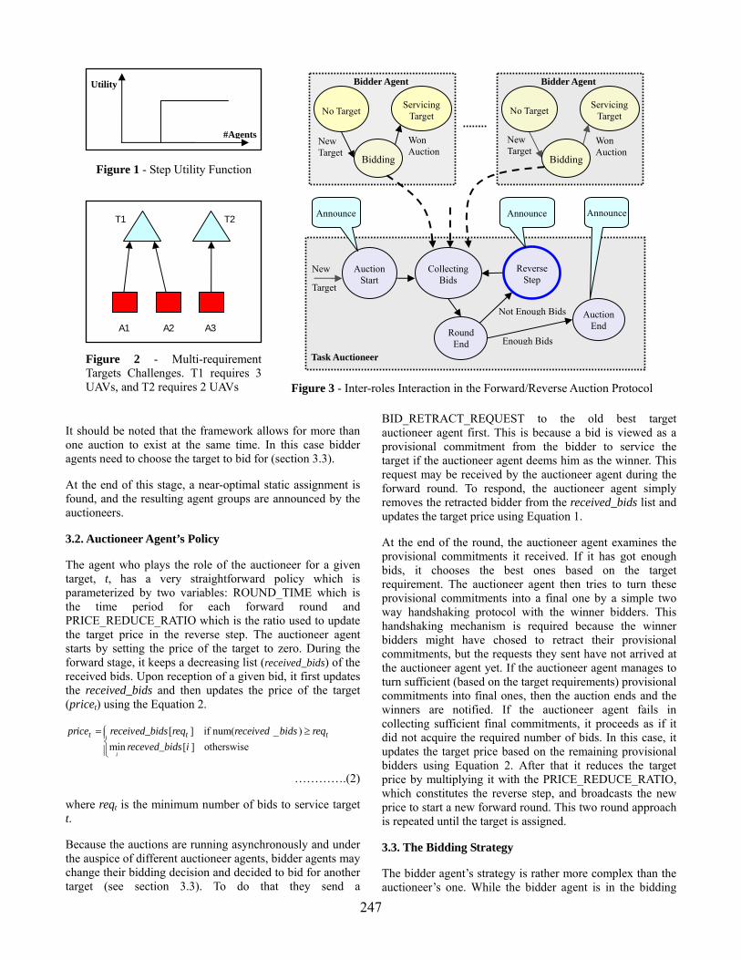
#Agents

A3 A1 A2

T2 T1

Figure 1 - Step Utility Function

Figure 2 - Multi-requirement Targets Challenges. T1 requires 3 UAVs, and T2 requires 2 UAVs

Utility

Bidding

Auction Start

Collecting Bids

Round End

Reverse Step

Auction End

Announce

Task Auctioneer

No Target

New Target

Servicing Target

Won Auction

Bidding

No Target

New Target

Servicing Target

Won Auction

New

Target

Announce Announce

Figure 3 - Inter-roles Interaction in the Forward/Reverse Auction Protocol

Not Enough Bids

Enough Bids

Bidder Agent Bidder Agent

It should be noted that the framework allows for more than one auction to exist at the same time. In this case bidder agents need to choose the target to bid for (section 3.3).

At the end of this stage, a near-optimal static assignment is found, and the resulting agent groups are announced by the auctioneers.

3.2. Auctioneer Agent’s Policy

The agent who plays the role of the auctioneer for a given target, t, has a very straightforward policy which is parameterized by two variables: ROUND_TIME which is the time period for each forward round and PRICE_REDUCE_RATIO which is the ratio used to update the target price in the reverse step. The auctioneer agent starts by setting the price of the target to zero. During the forward stage, it keeps a decreasing list (received_bids) of the received bids. Upon reception of a given bid, it first updates the received_bids and then updates the price of the target (pricet) using the Equation 2.

[ ] if num( _ ) min [ ] otherswise

i

t tprice received_bids req received bids reqreceved_bids i

= ⎧⎪⎨⎪⎩

t≥

auctioneer’s one. While the bidder agent is in the bidding

………….(2)

where reqt is the minimum number of bids to service target t.

Because the auctions are running asynchronously and under the auspice of different auctioneer agents, bidder agents may change their bidding decision and decided to bid for another target (see section 3.3). To do that they send a

BID_RETRACT_REQUEST to the old best target auctioneer agent first. This is because a bid is viewed as a provisional commitment from the bidder to service the target if the auctioneer agent deems him as the winner. This request may be received by the auctioneer agent during the forward round. To respond, the auctioneer agent simply removes the retracted bidder from the received_bids list and updates the target price using Equation 1.

At the end of the round, the auctioneer agent examines the provisional commitments it received. If it has got enough bids, it chooses the best ones based on the target requirement. The auctioneer agent then tries to turn these provisional commitments into a final one by a simple two way handshaking protocol with the winner bidders. This handshaking mechanism is required because the winner bidders might have chosed to retract their provisional commitments, but the requests they sent have not arrived at the auctioneer agent yet. If the auctioneer agent manages to turn sufficient (based on the target requirements) provisional commitments into final ones, then the auction ends and the winners are notified. If the auctioneer agent fails in collecting sufficient final commitments, it proceeds as if it did not acquire the required number of bids. In this case, it updates the target price based on the remaining provisional bidders using Equation 2. After that it reduces the target price by multiplying it with the PRICE_REDUCE_RATIO, which constitutes the reverse step, and broadcasts the new price to start a new forward round. This two round approach is repeated until the target is assigned.

3.3. The Bidding Strategy

The bidder agent’s strategy is rather more complex than the

247

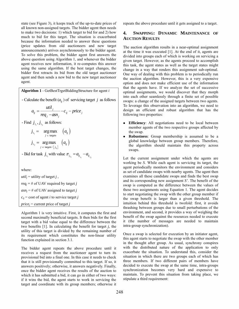
state (see Figure 3), it keeps track of the up-to-date prices of all known non-assigned targets. The bidder agent then needs to make two decisions: 1) which target to bid for and 2) how much to bid for this target. The situation is exacerbated because the information needed to answer these questions (price updates from old auctioneers and new target announcements) arrives asynchronously to the bidder agent. To solve this problem, the bidder agent first answers the above question using Algorithm 1, and whenever the bidder agent receives new information, it re-computes this answer using the same algorithm. If the best target changes, the bidder first retracts its bid from the old target auctioneer agent and then sends a new bid to the new target auctioneer agent.

Algorithm 1 - GetBestTrgetBiddingStructure for agent i

( )1 2

1

2

targets

targets

Calculate the benefit ( ) of servicing target as follows

- Find as follows:

-

,

argmax

argmax

ij

jij ij j

j j

i i

i ijj

ij

a j

utila c price

req asn

j j

j a

j∈

∈

= − −−

=

=

( )i1

1 1 1 2

\

Bid for task with value

- i i i

ijj

i j ij ij

a

j a aπ = −

where:

util = utility oj f target j ,

req = # of UAV required bj y target j

asn = # of UAV assigned to target j j

cij = cost of agent i to service target j

price = current price of target j j

Algorithm 1 is very intuitive. First, it computes the first and

The bidder agent repeats the above procedure until it

4. SWAPPING: DYNAMIC MAINTENANCE OF

The auction algorithm results in a near-optimal assignment

Efficiency: All negotiations need to be local between

s: Group membership is assumed to be a

Let the current assignment under which the agents are

Once a swap is selected for execution by an initiator agent,

second maximally beneficial targets. It then bids for the first target with a bid value equal to the difference between the two benefits [1]. In calculating the benefit for target j, the utility of this target is divided by the remaining number of its requirement which constitutes the non-linear utility function explained in section 3.1.

receives a request from the auctioneer agent to turn its provisional bid into a final one. In this case it needs to check that it is still provisionally committed to this target. If so, it answers positively; otherwise, it answers negatively. Finally, once the bidder agent receives the results of the auction to which it has submitted a bid, it can go in either of two ways: if it wins the bid, the agent starts to work in servicing the target and coordinate with its group members; otherwise it

repeats the above procedure until it gets assigned to a target.

AUCTION RESULTS

at the time it was executed [1]. At the end of it, agents are divided into groups each of which is working on servicing a given target. However, as the agents proceed to accomplish this task, the agent states as well as the target states might change in a way that renders this assignment sub-optimal. One way of dealing with this problem is to periodically run the auction algorithm. However, this is a very expensive option and does not make efficient use of the information that the agents have. If we analyze the set of successive optimal assignments, we would discover that they morph into each other seamlessly through a finite set of possible swaps: a change of the assigned targets between two agents. To leverage this observation into an algorithm, we need to design an efficient and robust algorithm that has the following two properties:

member agents of the two respective groups affected by the swap. Robustnesglobal knowledge between group members. Therefore, the algorithm should maintain this property across swaps.

working be S. While each agent is servicing its target, the agent periodically monitors the environment and considers as set of candidate swaps with nearby agents. The agent then examines all these candidate swaps and finds the best swap and its corresponding new assignment S’. The benefit of the swap is computed as the difference between the values of these two assignments using Equation 1. The agent decides to start negotiating the swap with the other group member if the swap benefit is larger than a given threshold. The intuition behind this threshold is twofold: first, it avoids thrashing between groups due to small perturbations of the environment, and second, it provides a way of weighing the benefit of the swap against the resources needed to execute it (the number of messages are needed to maintain intra-group synchronization).

this agent starts to negotiate the swap with the other member in the thought after group. As usual, synchrony conspires with the distributed nature of the application to only exacerbate the situation. To understand this, consider the situation in which there are two groups each of which has three members. If two different pairs of members have decided to execute the swap at the same time, intra-groups synchronization becomes very hard and expensive to maintain. To prevent this situation from taking place, we stipulate a third requirement:

248

Isolation: At any given time there can be at most one swap taking place between any two groups.

To achieve these requirements, an agent within each group is assigned to be the group leader. Let a swap take place between an initiator agent and an intended agent. The swap is then proceeds as follows:

1. Initialization - The initiator of the swap asks its group leader for permission to start a new swap. This permission is granted as long as there is no other swap taking place.

2. Asking for a swap - Upon reception of the swap permission from its own group leader, the initiator agent contacts the member agent involved in the swap in the other group to inform it about executing the swap.

3. Responding to the swap - Once the intended agent receives the swap request, it asks for permission from its own group leader. Based on its leader response (grant or decline), it informs the initiator with its decision (accept or decline).

4. Swap execution - Once the two parties agreed on the swap, each one informs its peers about the group update.

5. Finalization - After the initiator and intended agents inform their peers about the swap, they report to their group leaders that intra-group synchronization has been achieved.

As evident from the above procedure, a swap requires a large number of messages back and forth between group members; therefore the SWAP_THRESHOLD should be adjusted to take this into consideration. Currently, this threshold is treated as a pre-determined parameter to the framework, and its value is set based on a worst case analysis.

5. UAV AGENT ARCHITECTURE

This section provides a function-oriented specification of different components of an UAV agent used in the experimentation and the information flow between them. The emphasis here will be of the reasoning part of the agent.

Figure 4 depicts the UAV agent components as well as information flow between them. The central component of the agent architecture is the world model which is the main memory of the agent. It stores various kind of problem information at different levels of abstractions. The world model is feed with vision data from the communication module, and it provides various retrieval functions to other components of the agent. This allows these components to examine the world around the agent at the most suitable level of details for this component’s task.

The coordination module is the brain of the agent where all decisions are taken. It is responsible of sequencing the agent decision making process as well as coordinating the overall team members’ actions (team-level action sequencing). The main responsibility of this module is to decide the agent current mode of operation (rooming, bidding, or task

execution), and it also runs the auction framework as detailed before. It also stores partial coordination results on the world model like (which target I am currently committed to which group I am a member of, what is my role in this group, etc.) to be used by other modules.

UAV

Communication Module Robot Interface

World Model

Coordination Module

Target Handling

Object Info

Object Info

CoordinationResult

Object Info

Partial Decisions

Group Sync.

Movement Commands

Coordination Messages

Messages

Motion Planning / Collision Avoidance

Objects Info

Other Info

Objects UAVs

Figure 4 - Internal Architecture of a UAV Agent

The target handling and motion planning modules are responsible for materializing decisions of the coordination module. The responsibilities of these modules are to decide which point of the target to go to and to coordinate with other group members to avoid conflicts. This coordination is done by exchanging path-planning messages between group members through the communication module. Afterwards, the collision avoidance module monitors the world by examining the world model and make sure to avoid/prevent collisions using an A* algorithm [16].

6. EXPERIMENTAL RESULTS

Our main aim is to demonstrate our framework using a set of robot cars. Each car is controlled by an iPAQ and receives localization information from a leader vision server collaborating data from four vision servers, each of which is connected to a ceil-mounted vision camera. A vision server takes images from a camera and processes images searching for color plates mounted over the robot cars, which designate corresponding robots’ identification and headings. A leader vision server takes localization information from each vision server, and sends filtered and regulated localization information to iPAQs. Inter-agent communication is achieved via wireless communication between iPAQs. Different cars are used to represent UAVs and targets (see Figure 5). It is quite clear that this hardware setting would make discovering logical errors as well as tracing the agents’ behavior very hard. To deal with these issues, we developed a hardware/software shared agent code

249

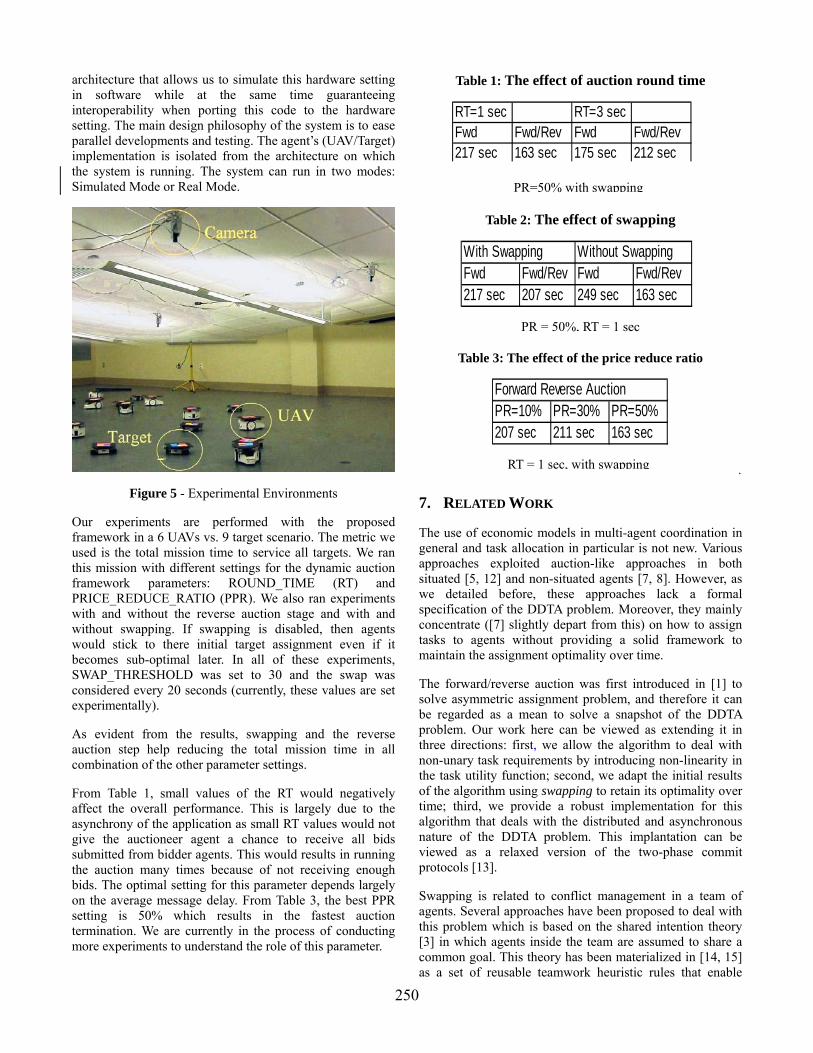
architecture that allows us to simulate this hardware setting in software while at the same time guaranteeing interoperability when porting this code to the hardware setting. The main design philosophy of the system is to ease parallel developments and testing. The agent’s (UAV/Target) implementation is isolated from the architecture on which the system is running. The system can run in two modes: Simulated Mode or Real Mode.

Figure 5 - Experimental Environments

Our experiments are performed with the proposed framework in a 6 UAVs vs. 9 target scenario. The metric we used is the total mission time to service all targets. We ran this mission with different settings for the dynamic auction framework parameters: ROUND_TIME (RT) and PRICE_REDUCE_RATIO (PPR). We also ran experiments with and without the reverse auction stage and with and without swapping. If swapping is disabled, then agents would stick to there initial target assignment even if it becomes sub-optimal later. In all of these experiments, SWAP_THRESHOLD was set to 30 and the swap was considered every 20 seconds (currently, these values are set experimentally).

As evident from the results, swapping and the reverse auction step help reducing the total mission time in all combination of the other parameter settings.

From Table 1, small values of the RT would negatively affect the overall performance. This is largely due to the asynchrony of the application as small RT values would not give the auctioneer agent a chance to receive all bids submitted from bidder agents. This would results in running the auction many times because of not receiving enough bids. The optimal setting for this parameter depends largely on the average message delay. From Table 3, the best PPR setting is 50% which results in the fastest auction termination. We are currently in the process of conducting more experiments to understand the role of this parameter.

Table 1: The effect of auction round time

RT=1 sec RT=3 secFwd Fwd/Rev Fwd Fwd/Rev217 sec 163 sec 175 sec 212 sec

PR=50% with swapping

Table 2: The effect of swapping

PR = 50%, RT = 1 sec

With Swapping Without SwappingFwd Fwd/Rev Fwd Fwd/Rev217 sec 207 sec 249 sec 163 sec

Table 3: The effect of the price reduce ratio

.

7. RELATED WORK

els in multi-agent coordination in

ced in [1] to

ted to conflict management in a team of

The use of economic modgeneral and task allocation in particular is not new. Various approaches exploited auction-like approaches in both situated [5, 12] and non-situated agents [7, 8]. However, as we detailed before, these approaches lack a formal specification of the DDTA problem. Moreover, they mainly concentrate ([7] slightly depart from this) on how to assign tasks to agents without providing a solid framework to maintain the assignment optimality over time.

The forward/reverse auction was first introdusolve asymmetric assignment problem, and therefore it can be regarded as a mean to solve a snapshot of the DDTA problem. Our work here can be viewed as extending it in three directions: first, we allow the algorithm to deal with non-unary task requirements by introducing non-linearity in the task utility function; second, we adapt the initial results of the algorithm using swapping to retain its optimality over time; third, we provide a robust implementation for this algorithm that deals with the distributed and asynchronous nature of the DDTA problem. This implantation can be viewed as a relaxed version of the two-phase commit protocols [13].

Swapping is relaagents. Several approaches have been proposed to deal with this problem which is based on the shared intention theory [3] in which agents inside the team are assumed to share a common goal. This theory has been materialized in [14, 15] as a set of reusable teamwork heuristic rules that enable

RT = 1 sec, with swapping

Forward Reverse AuctionPR=10% PR=30% PR=50%207 sec 211 sec 163 sec

250

agent teams to act reliably in dynamic situations. However, our work differs from these generic approaches as it was designed specifically to permeate seamlessly with our forward/reverse auction framework.

8. CONCLUSION AND FUTURE WORK

and conquer approach for the DDTA problem that deals separately with

n the same search and rescue domain using our Actor Architecture (AA) [17]

ed by the Defense Advanced Research Projects Agency under contract number

as and D.A. Castanon, “A Forward/reverse Auction Algorithm for Asymmetric Assignment Problems,”

S. Kulkarni, “Dynamic Distributed Resource Allocation: A Distributed

d joint action,” In Proceedings of the 12th International Joint

on Intelligent Systems and their Applications, 11(6):36-46,

oboCup Rescue Simulation Domain: A Short Note,” In Proceedings of the International Symposium

tion,” IEEE Transactions on Robotics and Automation, Special Issue on Multi-robot

Mobile Robots,” In Proceedings of IEE/RSJ International Workshop on

Robotics Institute Technical Report CMU-RI-TR-01-26, August 2001.

University of Massachusetts, May 1995.

cial Intelligence, 20:63-109, 1983.

s - Concepts and Design, 3rd edition, Addison-Wesley, 2001.

onitoring,” Journal of Artificial Intelligence Research, 12:105-147, 2000.

al Conference on Artificial Intelligence (AAAI), August 1997.

r Saddle River, NJ, 2003.

d Simulation for Studying UAV Coordination," 15th European Simulation Symposium (ESS 2003), pp.

In this paper we have presented a divide

its two main challenging aspects: combinatorial and dynamicity issues. To deal with the first issue we have adapted a forward reverse auction algorithm which was originally designed for bipartite maximal matching [1] to be suitable for the distributed, asynchronous, multi-requirement aspects of the DDTA problem. We have then proposed to use swapping as a mean to maintain the optimality of the initial auction results over time via chaining of local, communication-inexpensive negotiating steps. We have detailed the application of our approach in a UAV search and rescue domain and reported on early experimentations that prove the promise of our framework.

We plan to run large scale experiments o

which supports up to 10000 agents. We also plan to incorporate learning in our architecture to first tailor the agents’ bidding decisions and second to adapt the algorithm parameters to the environment dynamics in order to efficiently utilize the available bandwidth. Moreover, we will also contrast our approach with that in [2] and provide a principled way to contrast them in different settings. Finally, we also plan to investigate theoretically the optimally our multi-requirements extension to the auction algorithm.

ACKNOWLEDGMENT

This research is sponsor

F30602-00-2-0586. We would like to thank Hananeh Hajishirazi for implementing part of the collision avoidance and target handling modules. We would like also to thank Soham Mazumdar for early discussion on the forward/reverse auction algorithm.

REFERENCES

[1] D.P. Bertsek

Technical Report Lids-P-2159, MIT, 1993.

[2] P.J. Modi, H. Jung, M. Tambe, W. Shen,

Constraint Satisfaction Approach,” In Intelligent Agents VIII Proceedings of the International Workshop on Agents, Theories, Architectures, and Languages (ATAL’01), 2001.

[3] P.R. Cohen and H.J. Levesque, “Confirmation an

Conference on Artificial Intelligence, pages 951-957, 1991.

[5] K. Sycara, A. Pannu, M. Williamson, and D. Zeng, “Distributed Intelligent Agents,” IEEE Expert, Special Issue

December 1996.

[6] R. Nair, T. Ito, M. Tambe, and S. Marsella, “Task Allocation in the R

on RoboCup(RoboCup'01), 2001.

[7] B.P. Gerkey and M.J. Matarić, “Sold!: Auction Methods for Multi-robot Coordina

Systems, 18(6):758-768, October 2002.

[8] P. Caloud, W. Choi, J.-C. Latombe, C. Le Paper, and M. Yim, “Indoor Automation with many

Intelligent Robots and Systems, pages 67-72, 1990.

[10] M.B. Dias and A. Stentz, “A Market Approach to Multirobot Coordination,” Carnegie Mellon

[11] K.S. Decker, “Environment Centered Analysis and Design of Coordination Mechanisms,” Ph.D. Dissertation,

[12] R. Davis and R.G. Smith, “Negotiation as a Metaphor for Distributed Problem Solving,” Artifi

[13] G. Coulouris, J. Dollimore, and T. Kindberg. Distributed System

[14] G.A. Kaminka and M. Tambe, “Robust Agent Teams via Socially-attentive M

[15] M. Tambe, “Agent Architectures for Flexible, Practical Teamwork,” In Proceedings of the Nation

[16] S. Russell, P. Norvig, Artificial Intelligence: A Modern Approach, 2nd edition, Prentice Hall, Uppe

[17] M. Jang, S. Reddy, P Tosic, L. Chen, G. Agha. "An Actor-base

593-601, October 26-29, Delft, The Netherlands, 2003.

251

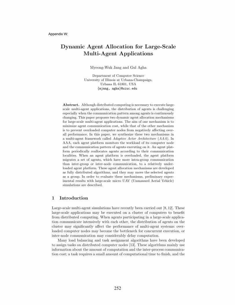
Dynamic Agent Allocation for Large-Scale

Multi-Agent Applications

Myeong-Wuk Jang and Gul Agha

Department of Computer ScienceUniversity of Illinois at Urbana-Champaign,

Urbana IL 61801, USAmjang, agha@uiuc.edu

Abstract. Although distributed computing is necessary to execute large-scale multi-agent applications, the distribution of agents is challengingespecially when the communication pattern among agents is continuouslychanging. This paper proposes two dynamic agent allocation mechanismsfor large-scale multi-agent applications. The aim of one mechanism is tominimize agent communication cost, while that of the other mechanismis to prevent overloaded computer nodes from negatively affecting over-all performance. In this paper, we synthesize these two mechanisms ina multi-agent framework called Adaptive Actor Architecture (AAA). InAAA, each agent platform monitors the workload of its computer nodeand the communication pattern of agents executing on it. An agent plat-form periodically reallocates agents according to their communicationlocalities. When an agent platform is overloaded, the agent platformmigrates a set of agents, which have more intra-group communicationthan inter-group or inter-node communication, to a relatively under-loaded agent platform. These agent allocation mechanisms are developedas fully distributed algorithms, and they may move the selected agentsas a group. In order to evaluate these mechanisms, preliminary exper-imental results with large-scale micro UAV (Unmanned Aerial Vehicle)simulations are described.

1 Introduction

Large-scale multi-agent simulations have recently been carried out [8, 12]. Theselarge-scale applications may be executed on a cluster of computers to benefitfrom distributed computing. When agents participating in a large-scale applica-tion communicate intensively with each other, the distribution of agents on thecluster may significantly affect the performance of multi-agent systems: over-loaded computer nodes may become the bottleneck for concurrent execution, orinter-node communication may considerably delay computation.

Many load balancing and task assignment algorithms have been developedto assign tasks on distributed computer nodes [13]. These algorithms mainly useinformation about the amount of computation and the inter-process communica-tion cost; a task requires a small amount of computational time to finish, and the

252

communication cost of tasks is known a priori. However, in many multi-agentapplications, agents do not cease from execution until their system finishes theentire operation [5]. Furthermore, since the communication pattern among co-operative agents is continuously changing during execution, it may be infeasibleto estimate the inter-agent communication cost for a certain time period. There-fore, task-based load balancing algorithms may not be applicable to multi-agentapplications.

This paper proposes two agent allocation mechanisms to handle the dynamicchange of the communication pattern of agents participating in a large-scalemulti-agent application and to move agents on overloaded computer nodes torelatively underloaded computer nodes. Adaptive Actor Architecture (AAA), theextended multi-agent framework of Actor Architecture [9], monitors the status ofcomputer nodes and the communication pattern of agents, and migrates agentsto collocate intensively communicating agents on a single computer node. Inorder to move agents to another computer node, an agent platform on a singlenode manages virtual agent groups whose member agents have more intra-groupcommunication than inter-group or inter-node communication. In order to evalu-ate our approach, large-scale micro UAV (Unmanned Aerial Vehicle) simulationsincluding 10,000 agents were tested.

This paper is organized as follows. Section 2 introduces the overall archi-tecture of our agent system. Section 3 explains in details two dynamic agentallocation mechanisms of our agent system. Section 4 shows the preliminaryexperimental results to evaluate these allocation mechanisms, and Section 5 de-scribes related work. Finally, Section 6 concludes this paper with our futurework.

2 Adaptive Actor Architecture

AAA provides a light-weight implementation of agents as active objects or actors[1]; agents in AAA are implemented as threads instead of processes, and theycommunicate using object messages instead of string messages. The actor modelprovides the fundamental behavior for a variety of agents; they are social andreactive, but they are not explicitly required to be “autonomous” in the sense ofbeing proactive [16]. However, autonomous actors may be implemented in AAA,and many of the applications used in our experimental studies require proactiveactors. Although the term agent has been used to mean proactive actors, for ourpurposes the distinction is not critical. In this paper, we use the terms ‘agent’and ‘actor’ as synonyms.

Adaptive Actor Architecture consists of two main parts:

– AAA platforms which provide the system environment in which agents existand interact with other agents. In order to execute agents, each computernode must have one AAA platform. AAA platforms provide agent statemanagement, agent communication, agent migration, agent monitoring, andmiddle agent services.

253

AAA Platform

Message Manager

Actor Manager Actor Migration Manager

Transport Receiver

Transport Receiver Transport Sender

Transport Sender

AAA Platform

Transport Manager

Transport Manager

Delayed Message Manager

Actor Allocation Manager

ATSpace

Actor

System Monitor

Fig. 1. Architecture of an AAA Platform

– Actor library which is a set of APIs that facilitate the development of agentson the AAA platforms by providing the user with a high level abstraction ofservice primitives. At execution time, the actor library works as the interfacebetween agents and their respective AAA platforms.

An AAA platform consists of ten components (see Fig. 1): Message Manager,Transport Manager, Transport Sender, Transport Receiver, Delayed MessageManager, Actor Manager, Actor Migration Manager, Actor Allocation Manager,System Monitor, and ATSpace.

The Message Manager (MM) handles message passing between agents. Everymessage passes through at least one Message Manager. If the receiver agent ofa message exists on the same AAA platform as the sender agent, the MM ofthe platform directly delivers the message to the receiver agent. However, if thereceiver agent is not on the same AAA platform, this MM delivers the messageto the MM of the platform where the receiver currently resides, and finallythe MM delivers the message to the receiver. The Transport Manager (TM)maintains a public port for message passing between different AAA platforms.When a sender agent sends a message to a receiver agent on a different AAAplatform, the Transport Sender (TS) residing on the same platform as the senderreceives the message from the MM of the sender agent and delivers it to theTransport Receiver (TR) on the AAA platform of the receiver. If there is no

254

built-in connection between these two AAA platforms, the TS contacts the TMof the AAA platform of the receiver agent to open a connection so that the TMcreates a TR for the new connection. Finally, the TR receives the message anddelivers it to the MM on the same platform.

The Delayed Message Manager (DMM) temporarily holds messages for mo-bile agents while they are moving from their AAA platforms to other AAAplatforms. The Actor Manager (AM) manages states of the agents that are cur-rently executing and the locations of the mobile agents created on the AAAplatform. The Actor Migration Manager (AMM) manages agent migration.

The System Monitor (SM) periodically checks the workload of its computernode and an Actor Allocation Manager (AAM) analyzes the communicationpattern of agents. With the collected information, the AAM makes decisions foreither agents or agent groups to deliver to other AAA platforms with the help ofthe Actor Migration Manager. The AAM negotiates with other AAMs to checkthe feasibility of migrations before starting agent migration.

The ATSpace provides middle agent services, such as matchmaking and bro-kering services. Unlike other system components, the ATSpace is implementedas an agent. Therefore, any agent can create an ATSpace, and hence, an AAAplatform may have more than one ATSpaces. The ATSpace created by an AAAplatform is called the default ATSpace of the platform, and all agents can ob-tain the agent names of default ATSpaces. Once an agent has the name of anATSpace, the agent may send the ATSpace messages in order to use its services,and the messages are delivered through the Message Manager.

3 Dynamic Agent Allocation

In order to develop large-scale distributed multi-agent applications, the multi-agent systems must be scalable. This scalability may be achieved if the appli-cation or the infrastructure does not include centralized components which canbecome a bottleneck. Moreover, the scalability requires relatively balanced work-load on computer nodes. Otherwise, the slowest node may become a bottleneck.However, balancing the workload between computer nodes requires significantoverhead: the relevant global state information needs to be gathered, and agentshave to transferred sufficiently frequently between computer nodes. Therefore,when the number of computer nodes and/or the number of agents is very large,load balancing is difficult to achieve. AAA uses the load sharing approach inwhich agents on an overloaded agent platform are moved to other underloadedagent platforms, but balanced workload among computer nodes is not required.

The third important factor for the scalability of multi-agent systems is thecommunication overhead. When agents on separate computer nodes communi-cate intensively with each other, this factor may significantly affect the per-formance of multi-agent systems. Even though the speed of local networks hasincreased considerably, the intra-node communication speed for agent messagepassing is much faster than inter-node communication. Therefore, if we can col-locate together agents which communicate intensively with each other, com-

255

munication time significantly decreases. It is not generally feasible for a userto distribute agents based on their communication pattern, because the com-munication pattern among agents may change over time in unpredictable ways.Therefore, agents should be reallocated dynamically according to their communi-cation patterns, and this procedure should be managed by a middleware system,such as agent platforms. Each agent platform in AAA monitors the status of itscomputer node and the communication pattern of agents on it, and the platformdynamically reallocates agents according to the information gathered.

3.1 Agent Allocation for Communication Locality

An agent allocation mechanism used in AAA handles the dynamic change of thecommunication pattern among agents. This mechanism consists of four phases:monitoring, agent allocating, negotiation, and agent migration (see Fig 2).

Agent Allocation

Monitoring

Negotiation

Agent Migration

Fig. 2. Four Phases for Basic Dynamic Agent Allocation

Monitoring Phase The Actor Allocation Manager checks the communicationpattern of agents under the support of the Message Manager. The Actor Allo-cation Manager makes a log with information about both the sender agent andthe agent platform of the receiver agent of each message. Therefore, each agentelement in the Actor Allocation Manager has variables representing all agentplatforms communicating with this agent; Mij is the number of messages sentfrom agent i to agent platform j.

Periodically or when requested by a system agent, the Actor Allocation Man-ager updates the communication pattern between agents and agent platformswith the following equation:

Cij(t) = α

(

Mij(t)∑

k Mik(t)

)

+ (1 − α)Cij(t − 1)

256

where Cij(t) is the communication dependency between agent i and agent plat-form j at the time step t; Mij(t) is the number of messages sent from agent i toagent platform j during the t-th time step; and α is a coefficient for the relativeimportance between recent information and old information.

For analyzing the communication pattern of agents, agents in AAA are clas-sified into two types: stationary and movable. Any agent in AAA can move itselfaccording to its decision, even though it is either stationary or movable. However,the Actor Allocation Manager does not consider stationary agents as candidatesfor agent allocation; an agent platform can migrate only movable agents. Thesetypes of agents are initially decided by agent programmers, and may be changedduring execution by the agents, but not by agent platforms.

Agent Allocation Phase After a certain number of repeated monitoringphases, the Actor Allocation Manager computes the communication dependencyratio of an agent between its current agent platform and another agent platform:

Rij =Cij

Cin, j = n

where Rij is the communication dependency ratio of agent i between its currentagent platform n and agent platform j.

When the maximum ratio of an agent is larger than a predefined threshold,the Actor Allocation Manager assigns this agent to a virtual agent group thatrepresents the remote agent platform:

max(Rij) > θ → ai ∈ Gj

where θ is the threshold for agent migration, ai represents agent i, and Gj meansagent group j.

When the Actor Allocation Manager has checked all agents and assigned someof them to agent groups, the Actor Allocation Manager starts the negotiationphase. After the agent allocation phase, information about the communicationdependency of agents is reset.

Negotiation Phase Before an agent platform migrates the agents that are inan agent group to another agent platform, the Actor Allocation Manager of thesender agent platform communicates with that of the destination agent plat-form to check its current status. If the destination agent platform has enoughspace and available computational resources for new agents, its Actor Alloca-tion Manager accepts the request for the agent group migration. Otherwise, thedestination agent platform sends the number of agents that it can accept. Thegranularity of this negotiation between agent platforms is an agent. When theActor Allocation Manager receives a reply from the destination agent platform,the Actor Allocation Manager sends as many agents to the destination agentplatform as the number of agents recorded in the reply message. When thenumber in the reply message is less than the number of agents in the virtual

257

group, the agents to be migrated are selected according to their communicationdependency ratios.

Agent Migration Phase When the destination agent platform can accept newagents, the Actor Allocation Manager of the sender agent platform initiates themigration of agents in the selected agent groups. After the current operation ofa selected agent finishes, the Actor Migration Manager moves the agent to thedestination agent platform decided by the Actor Allocation Manager. After theagent is migrated, the agent may restart its remaining operations.

3.2 Agent Allocation for Load Sharing

With the previous agent allocation mechanism, AAA handles the dynamic changeof the communication pattern of agents. However, this mechanism may increasethe workload of certain agent platforms. Therefore, our agent allocation hasbeen extended. When an agent platform is overloaded, the System Monitor de-tects this and activates the agent reallocation procedure. Since agents had beenassigned to their current agent platforms according to their communication pat-tern, choosing agents randomly to migrate to underloaded agent platforms mightresult in moving them back to their original agent platforms by the Actor Allo-cation Managers of their new agent platforms. This is because the moved agentsmay still have a high communication with their previous agent platform. Thisagent allocation mechanism consists of five phases: monitoring, agent grouping,group allocation, negotiation, and agent migration (see Fig 3).

Group Allocation

Agent Grouping

Monitoring

Negotiation

Agent Migration

Fig. 3. Five Phases for Extended Dynamic Agent Allocation

258

Monitoring Phase In the second agent allocation mechanism, the SystemMonitor periodically checks the state of its agent platform; the System Monitorgathers information about the current processor usage and the memory usage ofits computer node. When the System Monitor decides that its agent platform isoverloaded, it activates the agent allocation procedure. When the Actor Alloca-tion Manager is notified by the System Monitor, it starts monitoring the localcommunication pattern among agents and classifies them to agent groups. If anagent belonged to an agent group, it is assigned to this agent group; if an agentdid not belong to any agent group, it is randomly assigned to an agent group.The number of agent groups that exist on an agent platform is predefined.

For checking the communication pattern of agents, the Actor Allocation Man-ager makes a log with information about the sender agent, the agent platform ofthe receiver agent, and the agent group of the receiver agent of each message. Inaddition to the number Mij of messages sent from agent i to agent platform j,the number mik of messages sent from agent i to agent group k is updated whenthe receiver agent exists on the same agent platform. The summation of all mvariables of an agent is equal to the number of messages sent by the agent toits current agent platform:

∑

k mik = Min where the index of the current agentplatform is n.

After a predetermined time interval, or in response to a request from a sys-tem agent, the Actor Allocation Manager updates the communication patternbetween agents and agent groups on the same agent platform with the followingequation:

cij(t) = β

(

mij(t)∑

k mik(t)

)

+ (1 − β)cij(t − 1)

where cij(t) is the communication dependency between agent i and agent groupj at the time step t; mij(t) is the number of messages sent from agent i to agentsin agent group j during the t-th time step; and β is a coefficient for deciding therelative importance between recent information and old information.

Agent Grouping Phase After a certain number of repeated monitoring phases,each agent i is assigned to an agent group whose index is decided by arg

jmax (cij(t));

this group has the maximum value of the communication localities cij(t) of agenti. Since the initial group assignment of agents may not be well organized, themonitoring and agent grouping phases are repeated.

After each agent grouping phase, information about the communication de-pendency of agents is reset. During the agent grouping phase, the number ofagent groups can be changed. When two groups have much smaller populationsthan others, these two groups may be merged into one group. When one grouphas a much larger population than others, the agent group may be split intotwo groups. The minimum number and maximum number of agent groups arepredefined.

259

Group Allocation Phase After a certain number of repeated monitoring andagent grouping phases, the Actor Allocation Manager makes a decision to movean agent group to another agent platform. The group selection is based on thecommunication dependency between agent groups and agent platforms; the com-munication dependency Dij between agent group i and agent platform j is de-cided by the summation of the communication dependency between agents inthe agent group and the agent platform:

Dij =∑

k

Ckj(t) where ak ∈ Ai

where Ai represents the agent group i, and ak is a member agent of the agentgroup Ai.

The agent group which has the least dependency to the current agent plat-form is selected; the index of the group is decided by the following equation:

argj

max(

∑

j,j =n Dij

Din

)

where n is the index of the current agent platform. The destination agent plat-form of the selected agent group i is decided by the communication dependencybetween the agent group and agent platforms; the index of the destination plat-form is arg

jmax (Dij).

Negotiation Phase If one agent group and its destination agent platform aredecided, the Actor Allocation Manager communicates with that of the destina-tion agent platform. If the destination agent platform accepts all agents in thegroup, the Actor Allocation Manager of the sender agent platform starts themigration phase. Otherwise, this Actor Allocation Manager communicates withthat of the second best destination platform until it finds an available destinationagent platform or checks the possibility of all other agent platforms.

This phase of the second agent allocation mechanism is similar to that ofthe previous agent allocation mechanism, but there are some differences. Oneimportant difference between these two negotiation phases is the granularity ofnegotiation. If the destination agent platform has enough space and availablecomputation power for all agents in the selected agent group, the Actor Alloca-tion Manager of the destination agent platform accepts the request for the agentgroup migration. Otherwise, the destination agent platform refuses the request.The granularity of this negotiation between agent platforms is an agent group;the destination agent platform cannot accept part of an agent group.

Agent Migration Phase When the sender agent platform receives the accep-tance reply from the destination agent platform, the Actor Allocation Managerof the sender agent platform initiates the migration of agents in the selectedagent group. The procedure for the following phase in the second agent alloca-tion mechanism is the same as that of the previous agent allocation mechanism.

260

3.3 Characteristics

Transparent Distributed Algorithm These agent allocation mechanisms aredeveloped as fully distributed algorithms; each agent platform independentlyperforms its agent allocation mechanism according to information about itsworkload and the communication pattern of agents on it. There are no cen-tralized components to manage the overall procedure of agent allocation. Thesemechanisms are transparent to multi-agent applications. The only requirementfor application developers is to declare candidate agents for agent allocation asmovable.

Load Balancing vs. Load Sharing The second agent allocation mechanism isnot a load balancing mechanism but a load sharing mechanism; it does not try tobalance the workload of computer nodes participating in an application. The goalof our multi-agent system is to reduce the turnaround time of applications withoptimized agent allocation. Therefore, only overloaded agent platforms performthe second agent distribution mechanism, and agents are moved from overloadedagent platforms to underloaded agent platforms.

Individual Agent-based Allocation vs. Agent Group-based AllocationWith the agent group-based allocation mechanism, some communication local-ity problems may be solved. First, when two agents on the same agent platformcommunicate intensively with each other but not with other agents on the sameplatform, these agents may continuously stay on the current agent platform eventhough they have a large amount of communication with agents on another agentplatform. If these two agents can move together to the remote agent platform,the overall performance can be improved. However, an individual agent-basedallocation mechanism does not handle this situation. Second, individual agentallocation may require much platform-level message passing among agent plat-forms for the negotiation. For example, in order to send agents to other agentplatforms, agent platforms should negotiate with each other to avoid sendingtoo many agents to a certain agent platform, thus overloading the agent plat-form. However, if an agent platform sends a set of agents at one time, the agentplatforms may reduce negotiation messages and negotiation time.

Stop-and-Repartitioning vs. Implicit Agent Allocation Some object real-location systems require the global synchronization. This kind approach is calledthe stop-and-repartitioning [2]. Our agent distribution mechanisms are executedin parallel with applications. The monitoring and agent allocation phases do notinterrupt the execution of application agents.

Size of a Time Step In the monitoring phase, the size of each time step maybe fixed. However, this step size may be adjusted by an agent application. Forexample, in multi-agent based simulations, this size may be the same as the size

261

of a simulation time step. Thus, the size of time steps may be flexible accordingto the workload of each simulation step and the processor power. To use dynamicstep size, our agent system has a reflective mechanism; agents in applicationsare affected by multi-agent platform services, and the services of the multi-agentplatform may be controlled by agents in applications.

4 Experimental Results

For the purpose of evaluation, we provide experimental results related to microUAV (Unmanned Aerial Vehicle) simulations. These simulations include from2,000 to 10,000 agents; half of them are UAVs, and the others are targets. Mi-cro UAVs perform a surveillance mission on a mission area to detect and servemoving targets. During the mission time, these UAVs communicate with theirneighboring UAVs to perform the mission together. The size of a simulation timestep is one half second, and the total simulation time is around 37 minutes. Theruntime of each simulation depends on the number of agents and the collabora-tion policy among agents. For these experiments, we have used four computers(3.4 GHz Intel CPU and 2 GB main memory) with a Giga-bit switch.

For UAV simulations, the agent-environment interaction model has been used[3]; all UAVs and targets are implemented as intelligent agents, and the navi-gation space and radar censors of all UAVs are implemented as environmentagents.

To remove centralized components in distributed computing, each environ-ment agent on a single computer node takes charge of a certain navigation area.UAVs communicate directly with each other and indirectly with neighboringUAVs and targets through environment agents. Environment agents provide ap-plication agent-oriented brokering services with the ATSpace [10]. During sim-ulation, UAVs and targets move from one divided area to another, and UAVsand targets communicate intensively either directly or indirectly.

Fig. 4 depicts the difference of runtimes in two cases: dynamic agent alloca-tion, and static agent allocation. Fig. 5 shows the ratio of runtimes in both cases.These two figures show the potential performance benefit of dynamic agent allo-cation. In our particular example, as the number of agents is increased, the ratioalso generally increases. With 10,000 agents, the simulation using the dynamicagent allocation is more than five times faster than the simulation with a staticagent allocation.

5 Related Work

The mechanisms used in dynamic load balancing may be compared to those inAAA. Zoltan [7], PREMA/ILB [2], and Charm++ [4] support dynamic load bal-ancing with object migration. Zoltan uses a loosely coupled approach betweenapplications and load balancing algorithms using an object-oriented callbackfunction interface [7]. However, this library-based load balancing approach de-pends on information given by applications, and applications activate object

262

2000 4000 6000 8000 100000

10

20

30

40

50

60

Number of Agents (UAVs + Targets)

Run

time

(Hou

rs)

Static Agent AllocationDynamic Agent Allocation

Fig. 4. Runtime for Static and Dynamic Agent Allocation

2000 4000 6000 8000 100000

1

2

3

4

5

6

Number of Agents (UAVs + Targets)

Run

time

Rat

io

Fig. 5. Runtime Ratio of Static-to-Dynamic Agent Allocation

263

decomposition. Therefore, without developers’ through analysis about applica-tions, the change of dynamic access patterns of objects may not correctly bedetected, and object decomposition may not be performed at the proper time.The ILB of PREMA also interacts with objects using callback routines to collectinformation to be used for the load balancing decision making, and to pack andunpack objects [2]. Charm++ uses the Converse runtime system to maintainmessage passing among objects, and hence, the runtime system may collect in-formation to analyze communication dependencies among objects [4]. However,this system also requires callback methods for packing and unpacking objects asothers do. In AAA, the Actor Allocation Manager does not interact with agents,but it receives information from the Message Manager and the System Monitorto analyze the communication patterns of agents and the workload of its agentplatform. Also, developers do not need to define any callback method for loadbalancing.

J-Orchestra [15], Addistant [14], and JavaParty [11] are automatic appli-cation partitioning systems for Java applications. They transform input Javaapplications into distributed applications using a bytecode rewriting technique.They can migrate Java objects to take advantage of locality. However, they dif-fer from AAA in two ways. First, while they move objects to take advantage ofdata locality, AAA migrates agents to take advantage of communication locality.Second, the access pattern of an object differs from the communication patternof an agent. For example, although a data object may be moved whenever it isaccessed by other objects on different platforms, an agent cannot be migratedwhenever it communicates with other agents on different platforms. This is be-cause an object is accessed by another single object, but an agent communicateswith other multiple agents at the same time.

The Comet algorithm assigns agents to computer nodes according to theircredit [5]. The credit of an agent is decided by its computation load, intra-communication load, and inter-communication load. Chow and Kwok have em-phasized the importance of the relationship between intra-communication andinter-communication of each agent. However, there are some important differ-ences. The authors’ system includes a centralized component to make decisionsfor agent assignment, and their experiments include a small number of agents,i.e., 120 agents. AAA uses fully distributed algorithm, and experiments include10,000 agents. Because of the large number of agents, the Actor Allocation Man-ager cannot analyze the communication dependency among all individual agents,but only that between agents and agent platforms and that between agent groupsand agent platforms.

The IO of SALSA [6] provides various load balancing mechanisms for multi-agent applications. The IO also analyzes the communication pattern amongindividual agents. Therefore, it may not be applied to large-scale multi-agentapplications because of the large computational overhead.

264

6 Conclusion and Future Work

This paper has explained two dynamic agent allocation mechanisms used in ourmulti-agent middleware called Adaptive Actor Architecture; these agent alloca-tion mechanisms distributes agents according to their communication localitiesand the workload of computer nodes participating in large-scale multi-agent ap-plications. The main contribution of this paper is to provide agent allocationmechanisms to handle a large number of agents which communicate intensivelywith each other and change their communication localities. Because of the largenumber of agents, these agent allocation mechanisms focus on the communi-cation dependencies between agents and agent platforms and the dependenciesbetween agent groups and agent platforms, instead of the communication de-pendencies among individual agents. Our experimental results show that microUAV simulations using the dynamic agent allocation are approximately five timesfaster than those with a static agent allocation.

Our experiments suggest that increased load does not necessarily result in adecrease in the performance of multi-agent applications. If agents are properlylocated according to their communication pattern, the processor usage of theiragent platforms is quite high. Adding more computer nodes can increase theturnaround time of the entire computation; when the number of agent platformsfor an application exceeds a certain limit, the inter-node communication costbecomes larger than the benefit of distributed computing. Therefore, we plan todevelop algorithms to determine the appropriate number of agent platforms fora large-scale multi-agent application.

Acknowledgements

This research is sponsored by the Defense Advanced Research Projects Agencyunder contract number F30602-00-2-0586.

References

1. G. Agha. Actors: A Model of Concurrent Computation in Distributed Systems.MIT Press, 1986.

2. K. Barker, A. Chernikov, N. Chrisochoides, and K. Pingali. A Load BalancingFramework for Adaptive and Asynchronous Applications. IEEE Transactions onParallel and Distributed Systems, 15(2):183–192, February 2004.

3. M. Bouzid, V. Chevrier, S. Vialle, and F. Charpillet. Parallel Simulation of aStochastic Agent/Environment Interaction. Integrated Computer-Aided Engineer-ing, 8(3):189–203, 2001.

4. R.K. Brunner and L.V. Kale. Adaptive to Load on Workstation Clusters. In TheSeventh Symposium on the Frontiers of Massively Parallel Computation, pages106–112, February 1999.

5. K. Chow and Y. Kwok. On Load Balancing for Distributed Multiagent Computing.IEEE Transactions on Parallel and Distributed Systems, 13(8):787–801, August2002.

265

6. T. Desell, K. El Maghraoui, and C. Varela. Load Balancing of Autonomous Actorsover Dynamic Networks. In Hawaii International Conference on System SciencesHICSS-37 Software Technology Track, Hawaii, January 2004.

7. K. Devine, B. Hendrickson, E. Boman, M. St. Jhon, and C. Vaughan. Design ofDynamic Load-Balancing Tools for Parallel Applications. In Proceedings of theInternational Conference on Supercomputing, pages 110–118, Santa Fe, 2000.

8. L. Gasser and K. Kakugawa. MACE3J: Fast Flexible Distributed Simulation ofLarge, Large-Grain Multi-Agent Systems. In Proceedings of the First InternationalConference on Autonomous Agents & Multiagent Systems (AAMAS), pages 745–752, Bologna, Italy, July 2002.

9. M. Jang and G. Agha. On Efficient Communication and Service Agent Discoveryin Multi-agent Systems. In Third International Workshop on Software Engineer-ing for Large-Scale Multi-Agent Systems (SELMAS ’04), pages 27–33, Edinburgh,Scotland, May 24-25 2004.

10. M. Jang, A. Abdel Momen, and G. Agha. ATSpace: A Middle Agent to SupportApplication-Oriented Matchmaking and Brokering Services. In IEEE/WIC/ACMIAT(Intelligent Agent Technology)-2004, pages 393–396, Beijing, China, September20-24 2004.

11. M. Philippsen and M. Zenger. JavaParty - Transparent Remote Objects in Java.Concurrency: Practice and Experience, 9(11):1225–1242, 1997.

12. K. Popov, V. Vlassov, M. Rafea, F. Holmgren, P. Brand, and S. Haridi. ParallelAgent-Based Simulation on a Cluster of Workstations. Parallel Processing Letters,13(4):629–641, 2003.

13. P.K. Sinha. Chapter 7. Resource Management. In Distributed Operating Systems,pages 347–380. IEEE Press, 1997.

14. M. Tatsubori, T. Sasaki, S. Chiba, and K. Itano. A Bytecode Translator for Dis-tributed Execution of ’Legacy’ Java Software. In Proceedings of the 15th EuropeanConference on Object-Oriented Programming (ECOOP), pages 236–255, Budapest,June 2001.

15. E. Tilevich and Y. Smaragdakis. J-Orchestra: Automatic Java Application Parti-tioning. In Proceedings of the 16th European Conference on Object-Oriented Pro-gramming (ECOOP), Malaga, June 2002. http://j-orchestra.org/.

16. M. Wooldridge. An Introduction to MultiAgent Systems. John Wiley & Sons, Ltd,2002.

266

Maximal Clique Based Distributed Group FormationFor Task Allocation in Large-Scale Multi-Agent Systems

Predrag T. Tosic and Gul A. Agha

Open Systems Laboratory, Department of Computer ScienceUniversity of Illinois at Urbana-Champaign

Mailing address: Siebel Center for Computer Science,201 N. Goodwin Ave., Urbana, IL 61801, USA

p-tosic@cs.uiuc.edu, agha@cs.uiuc.edu

Abstract. We present a fully distributed algorithm for group or coalition formation among autonomous agents. The al-gorithm is based on two main ideas. One is a distributed computation of maximal cliques (of up to pre-specified size) inthe underlying graph that captures the interconnection topology of the agents. Hence, given the current configuration ofthe agents, the groups that are formed are characterized by a high degree of connectivity, and therefore high fault toler-ance with respect to node and link failures. The second idea is that each agent chooses its most preferable coalition basedon how highly the agent values each such coalition in terms of the coalition members’ combined resources or capabili-ties. Coalitions with sufficient resources for fulfilling particular highly desirable task(s) are preferable to coalitions witheither insufficient resources, or with resources that suffice only for completing less valuable tasks. We envision variantsof our distributed algorithm herein to prove themselves useful coordination subroutines in many massively multi-agentsystem applications where the agents may repeatedly need to form temporary groups or coalitions of modest sizes in anefficient, online and fully distributed manner.

Keywords: distributed algorithms, large-scale multi-agent systems, distributed group formation, agent coalitions

1 Introduction and Motivation

Autonomous agents and multi-agent systems (MAS) [1, 4, 29, 30] are characterized, among other properties, by (i) aconsiderable degree of autonomy of individual computing entities or processes (agents) and, at the same time, the fact that(ii) each agent has a local, that is, in general, incomplete and imperfect “picture of the world”. Since in MAS there is eitherno central control, or at best only a limited central control, and the individual agents have to both think and act locally,genuinely distributed algorithms are needed for the agents to effectively coordinate with one another.

MAS pose a number of challenges to a distributed algorithm designer. Many of the major challenges are related tovarious aspects of the agent coordination problem (e.g., [1, 29]). In order to be able to effectively coordinate, agentsneed to be able to reach consensus (or agreement) on various matters of common interest. Two particularly prominentdistributed consensus problems are those of leader election (e.g., [8, 22]) and group formation. Group or coalitionformation is an important issue in distributed systems in general [8], and MAS in particular [33]. Given a collection ofcommunicating agents, the goal in distributed group formation is that these agents, based on their local knowledge only,decide how to effectively split up into several groups, so that each agent knows which group(s) it belongs to.

There are several critical issues that a MAS designer needs to address in the context of (distributed) group formation.First, what is the right notion of a group in a given setting? Second, a distributed group formation mechanism - that is,a distributed algorithm that enables agents to effectively form groups or coalitions - needs to be provided. Third, groupsand each agent’s knowledge about its group membership need to be maintained and, when needed, appropriately updated.Fourth, are the groups to be allowed to overlap, so that an agent may simultaneously belong to two or more groups? Theseand other challenges related to autonomous agents forming coalitions have been extensively studied in the literature on

267

multi-agent systems, e.g., [9, 11, 14, 18, 19, 33]. They have also arisen in our own recent and ongoing work on parametricmodels and a scalable simulation of large scale (

agents) ensembles of autonomous unmanned vehicles on a

multi-task mission [6, 7, 23, 24].Herein, we restrict our attention to the second issue above. We propose a particular mechanism (distributed algorithm)

for an effective coalition formation that ensembles of autonomous agents can use as one of their basic coordination subrou-tines. A need for a dynamic, fully distributed, efficient and online group formation may arise due to a number of differentfactors, such as the geographical dispersion of the agents, heterogeneity of tasks and their resource requirements, hetero-geneity of agents’ capabilities, and so on [24]. While for small- and medium-scale systems of robots or unmanned vehiclesa fully or partially centralized approach to group formation and maintenance may be feasible or even optimal, large scalesystems (with the number of agents of orders of magnitude

or higher) appear to necessitate a fully distributed

approach. That is, the agents need to be able to self-organize into coalitions, and quickly reach a consensus on who isforming a coalition with whom in a fully decentralized manner [25].

2 Group or Coalition Formation in Multi-Agent Systems

Large ensembles of autonomous agents provide an important class of examples where the agents’ capability to coordinateand, in particular, to self-organize into groups or coalitions, is often of utmost importance for such systems to be able toaccomplish their tasks.

One can distinguish between two general, broad classes of such autonomous agents. One is the class of agents deployedin the context of distributed problem solving. The agents encountered in distributed problem solving (DPS) typically sharetheir goal(s). For instance, DPS agents most often have a joint utility function that they all wish to maximize as a team,without any regard to (or perhaps even a notion of) individual payoffs. This joint utility or, more generally, the goal or setof goals assigned to DPS agents, is usually provided by their designer. However, it may not be always feasible - or evenpossible - that the designer always explicitly specify, for instance, how are the agents to divide-and-conquer their tasksand resources, how are they to form groups and elect leaders of those groups, etc. Due to scalability, incomplete a prioriknowledge of the environments these agents may encounter, and possibly other considerations, instead of “hard-wiring”into his DPS agents explicitly how are the agents to be coordinated, the system designer may choose only to enable theautonomous agents with the basic coordination primitives, and leave to the agents to self-organize and coordinate as thesituation may demand. Hence, in many situations the DPS agents may be required to be able to effectively form groups orcoalitions in a fully distributed manner.

The second basic type of agents, the self-interested agents, are a kind of agents that do not share their goals (and,indeed, need not share their designer). In contrast to the DPS agents, each self-interested agent has its own agenda (e.g., anindividual utility function it is striving to maximize), and no altruistic incentives to cooperate with other agents. However,even such self-interested, goal-driven or individual-utility-driven agents, while in essence selfish, may nonetheless stillneed to cooperatively coordinate and collaborate with each other in many situations. One class of examples are thoseagents (such as, e.g., autonomous unmanned vehicles) that, if they do not coordinate in order to resolve possible conflicts,they risk mutual annihilation. Another class of examples are the agents with bounded resources: individually, an agent maylack resources to accomplish any of its desired tasks - yet, if this agent forms a coalition with one or more other agents, thecombined resources and joint effort of all agents in such a coalition may provide utility benefits to everyone involved. Anexample are heterogeneous types of agents deployed to a rescue mission in a disaster area: while there is an overarching,global goal at the system level, each agent typically also has its local, individual notion of task(s) and its own goal(s).

For these reasons, group and coalition formation are of considerable interest for many different kinds of autonomousagents and multi-agent systems, and, among other, even in those multi-agent systems where the agents do not share aglobal utility function, and where each agent generally acts selfishly. In particular, efficient fully distributed algorithms foreffective group formation are needed. Such algorithms should use only a few communication rounds among the agents,

268

place a very modest computational burden on each agent, and ensure that a distributed consensus among the agents on whois forming a group with whom is effectively, reliably and efficiently reached.

We propose herein one such class of distributed algorithms. We describe the generic, distributed group (coalition)formation algorithm in Section 4 and give the pseudo-code in the Appendix. Variations of this basic max-clique-basedgroup formation algorithm can be designed to meet the needs of various types of agents, such as, to give some examples,the following:

- the classical cooperative DPS agents [9, 10, 18, 19];- different kinds of self-interested, either strictly competing or competing-and-cooperating agents [14, 24] where con-

cepts, paradigms and tools from N-person game theory have found many applications; and, more generally,- various bounded-resource, imperfect-knowledge agents acting in complex environments (e.g., [24, 30]) that are typi-

cally only partially accessible to any agent; such autonomous agents are thus characterized by bounded rationality [20].We propose herewith a generic distributed group formation algorithm based on the idea that, in peer-to-peer (in par-

ticular, leaderless) MAS, an agent (node) would prefer to form a group with those agents that it can communicate withdirectly, and, moreover, where every member of such a potential group can communicate with any other member directly.That is, the preferable groups (coalitions) are actually (maximal) cliques. It is well-known that finding a maximal clique inan arbitrary graph is NP-complete in the centralized setting [3, 5]. This implies the computational hardness that, in general,each node faces when trying to determine maximal clique(s) it belongs to. However, if the degree of a node (that is, itsnumber of neighbors in the graph) is small, in particular, if it is , then finding all maximal cliques this node belongs tois computationally feasible. If one cannot guarantee that, or a priori does not know if, all the nodes in a given underlyingMAS interconnection topology are of small degree, then one has to impose additional constraints in order to ensure that theagents are not attempting to solve an infeasible problem. In particular, we shall additionally require herein that the possiblecoalitions to be formed, be of up to a certain pre-specified maximum size.

One may ask, why would this, maximal-clique based approach be promising for the very large scale (or massive) multi-agent systems (MMAS) that may contain ensembles of anywhere from thousands to millions of agents? The underlyinggraph (network topology) of such MMAS is bound to be very large, thus, one may argue, rendering even many typicallyefficient (i.e., polynomial-time in the number of agents) algorithms obsolete due to their prohibitive cost, let alone allowingdistributed coordination strategies that are based on the graph theoretic algorithms that are themselves, in the classical,centralized setting, NP-complete in general. However, there is one critical observation that saves the day of the approachthat we propose herewith: even if the underlying graph of an MMAS is indeed very large (possibly millions of nodes), inmany important applications this graph will also tend to be very sparse. That is, a typical, average node (agent) will tend tohave only a handful, and almost certainly only neighbors. Therefore, a distributed algorithm where agents act, reasonand communicate strictly locally, where no flooding of the network is ever performed (or needed), and where each nodeneeds to store and work with only the data pertaining to its near-by nodes, can still be designed to be sufficiently efficient.

Some examples of the engineering, socio-technical and socio-economic systems and infrastructures that can be modeledas MMAS and that are also characterized by the aforementioned sparseness of the underlying network topology, includethe following:

(i) Large-scale (

) ensembles of micro-UAVs (or other similar autonomous unmanned vehicles) deployed, forexample, in a surveillance or a search-and-rescue mission over a sizable geographic area. Unlike the scenarios where dozensof macro UAVs are employed, where a centralized control and/or one human operator per UAV are affordable and perhapsthe most efficient and robust way of deployment, in a very large-scale system of UAVs no central control is feasible or evenpossible, and the run-time human intervention is either minimal or nonexistent. Such micro-UAV ensembles, therefore,need to be able to coordinate, self-organize, and self-adapt to the changing environments in a truly decentralized, dynamicand autonomous manner. For more on design and simulation challenges of such large-scale ensembles of (micro-)UAVs,see, e.g., [6, 23, 24].

(ii) Smart sensor networks that include anywhere from thousands to millions of tiny sensors, each of which often of

269

only a few millimeters in size, and of a rather limited computational and communication power. In particular, the RAMmemory of such sensors is currently typically of the order of Kilobytes, the flash memory range is about

, the

communication bandwidth is

Kilobits/second, and a typical battery life span is anywhere from a few hoursup to a week. Such smart sensors usually communicate via essentially local broadcasts with very limited ranges. Themain “communication mode” of the agents in our algorithm in Section 4 will be precisely the local broadcasts. Also,due to small memory capacities and low power consumption requirements, smart sensors, in order to be effective, have tosimultaneously minimize both the amount of local processing, and how much (and how often) they communicate messagesto other sensors. Sensor networks, although on a much smaller scale, have already been used as an example to whichdynamic distributed constraint satisfaction/optimization formalisms can be fruitfully applied [10].

(iii) Various social networks, and, in particular, various variants of ’small-world’ networks where, in addition to strictlylocal connectivity in the communication network topology, a relatively few long-range connections are randomly added[27, 28]. A typical node in such a network will have only a handful of neighbors it can directly communicate with, and,moreover, most or nearly all of these neighbors in the network will also tend to be the neighbors in the usual, physicalproximity sense.

(iv) Various socio-technical infrastructures, such as, e.g., traffic and transportation systems, power grids, etc. For asimple concrete example, consider a car driver (an autonomous agent) participating in the traffic in a large city. While theremay be millions of such drivers on the road at the same time, the decision-making of a driver-agent is based, for the mostpart , on a few properties of its local environment, i.e., the actions of near-by agents; likewise, his own actions will usuallydirectly affect only a handful of other agents in the system (e.g., the driver right behind him, or the pedestrian trying to crossthe street right ahead of him). Thus, when modeling and simulating such an infrastructure with an appropriate large-scalenetwork and a MMAS, the underlying network, while of a very large size, will be in general fairly sparse, and a typicalnode adjacent to (meaning, in this context, capable of directly affecting and/or perceiving) only a small number of othernodes. An ambitious project on realistic, large-scale modeling and simulation of infrastructures such as city traffic systems,called TRANSIMS, is described at [26] and in the documents found therein.

We now return to the dynamic, distributed group or coalition formation in massively multi-agent systems, and themathematical formalisms and algorithmic solutions proposed for this challenging problem. A variety of coalition formationmechanisms have been proposed in the MAS literature both in the context of DPS agents that are all sharing the same goal(as, e.g., in [19]) and in the context of self-interested agents where each agent has its own individual agenda (as, e.g., in[18, 33]). In particular, the problem of distributed task or resource allocation, and how is this task allocation coupled towhat coalition structures are (most) desirable in a given scenario [9, 19], are also of central importance in our own workon a concrete MAS application with a particular type of robotic agents, namely, unmanned aerial vehicles (UAVs), that areresiding and acting in bounded resource multi-task environments [6, 23, 24].

Another body of MAS literature highly relevant to our central problem herein, namely distributed coalition forma-tion and task and/or resource allocation, casts the distributed resource allocation problems into the distributed constraintsatisfaction and/or optimization (DCS/DCO) terms [9, 10, 11].

Of the particular relevance to our work herein and other possible extensions of the original maximal clique based groupformation algorithm presented in [25] are references [19] and [10]. While Modi et al. in [10] offer the most completeformalization of various distributed resource and/or task allocation problems and general mappings to appropriate types orsubclasses of (dynamic) distributed constraint problems, two characteristics of their approach make it unsuitable for a directapplication to our modeling framework of massively multi-agent systems in general (see, e.g., [24]), and the applicationdomains we had in mind when devising the algorithm presented herein, in particular.

One, the agents in [10] are strictly cooperative, share the same goals, and have no notion of individual utilities orpreferences. While we have studied cooperative MAS in [24] and elsewhere, as well, one of our main assumptions is that,

There are exceptions of course; for instance, when an imminently approaching tornado is announced on the radio.

270

due to a large scale of the system and a high dynamism and unpredictability of the changes in the environment and the goals,no shared or global knowledge of the environment or the goals is maintained, and, in particular, each agent has its ownindividual preferences over the possible (local) states of the world. The collaboration is then achieved through “encoding”incentives into the individual agents’ individual behavior functions [23], and thus using the incentive engineering approach[2] to enable the agents to cooperatively coordinate even though each agent is, strictly speaking, self-interested.

Two, we address the issue of which agents will select which tasks to serve [23, 24], or, as in this paper, which groups ofagents will form in order to serve some particular set of tasks. To that end, what is critical is an agent’s or agent coalition’scapabilities for serving the desired task(s). Each agent possesses a tuple of capabilities or available resources; likewise, eachtask has a tuple of resource requirements. An agent coalition can serve a particular task if and only if each component (i.e.,individual capability or resource) of its joint tuple of capabilities is greater than or equal to the corresponding requirementvector entry of that task. An agent can only belong to one coalition at a time, and work with its fellow coalition members onone task at a time. Thus, while the agent operations in [10] are mutually exclusive with respect to time (an agent can onlyexecute a single operation at any time), our agent capabilities are mutually exclusive with respect to space or, equivalently,task allocation. Clearly, a complete model of resource and task allocation in MMAS should incorporate both aspects.Since we are presently only interested in coalition formation for the purpose of coalition-to-task mapping, but we are notconcerned herein with how are then these agent coalitions exactly going to perform the tasks they have been mapped to,our framework as described in [24] and outlined herein suffices for the current purposes.

The importance of DCS in MAS in general is discussed, e.g., in [32]. However, further discussion of DCS basedapproaches to distributed resource or task allocation and coalition formation is beyond the scope of this paper.

3 Problem Statement and Main Assumptions

The main purpose of this work is a generic, fully distributed, scalable and efficient algorithm for ensembles of autonomousagents to use as a subroutine - that is, as a part of their coordination strategy - with a purpose of efficiently formingtemporary groups or coalitions.

The proposed algorithm is a graph algorithm. The underlying undirected graph

captures the communication (ad hoc)network topology among the agents, as follows. Each agent is a node in the graph. As for the edges, the necessary require-ment for an edge between two nodes to exist is that the two nodes be able to directly communicate with one another atthe time our distributed group formation subroutine is called. That is, an unordered pair of nodes is an edge of theunderlying graph if and only if can communicate messages to

, or

can communicate messages to , or both.

.

The basic idea is to efficiently partition this graph into (preferably, maximal) cliques of nodes. These maximal cliqueswould usually also need to satisfy some additional criteria in order to form temporary coalitions of desired quality. Thesecoalitions are then maintained until they are no longer useful or meaningful. For instance, the coalitions should be trans-formed (or else simply dissolved) when the interconnection topology of the underlying graph considerably changes, eitherdue to the agents’ mobility, or because many old links have died out and perhaps many new, different links have formed,

For simplicity, we assume the graph is undirected, even though the communication from one node to another is clearly directional,and the communication links need not be symmetric. However, since the nodes eventually need to reach a mutual consensus, whichrequires that all members of a coalition agree to the same coalition and notify all other coalition members of the agreement, theassumption about the edge (non-)directionality is inconsequential, in a sense that only those coalitions that indeed are cliques in thecorresponding directed graph will ever be agreed upon by the agents.We point out that this definition of the graph edges can be made tighter by imposing additional requirements, such as, e.g., that thetwo agents (that is, graph nodes), if they are to be connected by an edge, also need to be compatible, for instance, in terms of theircapabilities, that they each provide some resource(s) that the other agent needs, and/or the like.

271

and the like. Another possible reason to abandon the existing coalition structure is when the agents determine that the coali-tions have accomplished the set of tasks that these coalitions were formed to address. Thus, in an actual MAS application,the proposed group formation algorithm may need to be invoked a number of times as a coordination subroutine.

We assume that each agent has a locally accurate (see, e.g., discussion in [24]) picture of (i) who are its neighboringagents, and (ii) what are the near-by tasks and, in particular, what are these tasks’ resource requirements. Each agent isequipped with a tuple of its internal resources, or capabilities [19]. Each task requires certain amount of each of theindividual resources in this tuple in order to be serviced. A single agent, or a coalition of two or more agents, can serve aparticular task if and only if their joint capabilities suffice with respect to the task’s resource consumption requirements.That is, the sum of each component of the capability vector taken over all the agents in the coalition has to be greater than,or equal to, the corresponding component of the task’s resource consumption vector.

Our distributed max-clique based group formation algorithm is sketched in the next section. For this algorithm to beapplicable, the following basic assumptions need to hold:

- Agents communicate with one another by exchanging messages either via local broadcasts, or in a peer-to-peerfashion.

- Communication bandwidth availability is assumed not to be an issue.- Each agent has a sufficient local memory for storing all the information received from other agents.- Communication is reliable during the group formation, in the following sense: if an agent, , sends a message to

another agent

(either via a local broadcast where it is assumed that

is within the communication range of , or in adirect, peer-to-peer manner), either agent

gets exactly the same message that has sent, or else the communication link

has completely failed and so

does not receive anything from at all. In particular, we assume no scrambled or otherwisemodified messages are ever received by any receiving agent. Also, once the groups are formed, the above assumption oncommunication reliability need no longer hold

.

- Each agent has (or else can efficiently obtain) a reliable knowledge of which other agents are within its communicationrange.

- Each agent, i.e., each network node, has a unique global identifier, ’UID’, and the agent knows its UID.- There is a total ordering, , on the set of UIDs, and each agent knows this ordering .- Each agent uses time-outs in order to place an upper bound on for how long it may be waiting to hear from any other

agent. If agent has sent a message (e.g., a coalition proposal - see Section 4 ) to agent

, and the latter is not respondingat all, there are three possibilities: (i) agent

has failed; (ii) communication link from

to has failed; or (iii) while

is in ’s communication range, vice versa actually does not hold (but may not know it).- The veracity assumption holds, i.e., an agent can trust the information about tasks, capabilities, etc. it receives from

other agents.To summarize, when agent sends a message to

, then

either receives exactly what had sent, or nothing at

all - and, moreover, if

has received the message,

knows that is telling the truth about its neighbors, capabilities,commitments and preferences in it (see Appendix).

On the other hand, an agent need not a priori know the UIDs of any of the other agents, or, indeed, how many otheragents are present in the system at any time.

In addition to its globally unique identifier UID, which we assume is a positive integer, and the vector of capabilities,each agent has two local flags that it uses in communication with other agents. One of the flags is the binary “decision flag”,which indicates whether or not this agent has already joined some group (coalition). Namely, , andthe value of this flag is

as long as the agent still has not irrevocably committed to what coalition it is joining. The second

flag is the “choice flag”, which is used to indicate to other agents, how “happy” the agent is with its current tentative choice

As this requirement is still restrictive, and considerably limits the robustness of our algorithm, we will try to relax this assumptionin our future work, and enable the agents to effectively form groups even in the presence of some limited amount of communicationnoise during the group formation process.

272

or proposal of the group to be formed. That is, the choice flag indicates the level of an agent’s urgency that its proposal fora particular coalition to be formed be accepted by the neighbors to whom this proposal is being sent. For more details, werefer the reader to Appendix and reference [25].

4 An Outline of Max-Clique-Based Distributed Group Formation for Task Allocation

Now that the assumptions have been stated and the notation has been introduced, we outline our distributed maximal cliquebased coalition formation algorithm. We describe in some detail how the algorithm works below; the pseudo-code is givenin Appendix.

The proposed distributed group or coalition formation algorithm is based on two main ideas. One idea, familiar fromthe literature (see, e.g., [19] and references therein), is to formulate a distributed task and/or resource allocation problemas a (distributed) set covering problem, (D)SC, in those scenarios where group overlaps are allowed, or a (distributed)set partitioning problem, (D)SP, when no group overlaps are allowed. Two (or more) groups overlap if there exists anelement that belongs to both (all) of them. It is well-known that decision versions of the classical, centralized versions ofthe SC and SP problems are NP-complete [5]. Hence, we need efficient (distributed) heuristics so that the agents caneffectively deploy DSC- or DSP-based strategies for coalition formation. Fortunately, some such efficient heuristics arealready readily available [19].

The second main idea is to ensure that the formed groups of agents meet the robustness and fault tolerance criteria,which are particularly important in applications where there is a high probability of node and/or communication linkfailures. Indeed, we were primarily motivated by such applications when designing the algorithm proposed herewith (see[23, 24]). The most robust groups of agents of a particular size are those that correspond to cliques in the underlyinginterconnection topology of the agents’ communication network. Moreover, the larger such a clique, the more robust thegroup of agents in the clique with respect to the node and/or link failures. Hence, appropriate maximal cliques need tobe formed in a distributed fashion. However, the Maximal Clique problem is also well-known to be NP-hard [3, 5]. Thishardness stems from the fact that an agent, in the general case (arbitrary underlying graph), may need to test for “cliqueness”exponentially many candidate subsets that it belongs to. However, in graphs where the maximum degree of each node isbounded by , where is a constant and is the total number of nodes in the graph, the number of subsets that eachnode belongs to, and therefore the number of candidate cliques, is , i.e., polynomial in the total number of nodes, . In particular, in sufficiently sparse graphs, where the node degrees are bounded by some (small) constant, ,the size of any maximal clique cannot exceed . In such situations, since is presumably still sufficiently small, findingmaximal cliques becomes both theoretically feasible (i.e., solvable in the time polynomial in the number of agents) andpractically computable in the online, real-time scenarios that are of main interest in MMAS applications .

We approach distributed coalition or group formation for task allocation as follows. The “candidate coalitions” aregoing to be required (whenever possible) to be cliques of modest sizes. That is, the system designer, based on the applicationat hand and the available system resources (local computational capabilities of each agent, bandwidth of agent-to-agentcommunication links, etc.), a priori chooses a threshold, , such that only coalitions of sizes up to are considered.Agents themselves subsequently form groups in a fully distributed and online manner, as follows. Each agent (i) firstlearns of who are its neighbors, then (ii) determines appropriate candidate coalitions, that the agent hopes are (preferablymaximal, but certainly of size bounded by ) cliques that it belongs to, then (iii) evaluates the utility value of each suchcandidate coalition, measured in terms of the joint resources of all the potential coalition members, then (iv) chooses themost desirable (highest utility value to the agent) candidate coalition, and, finally, (v) sends this choice to all its neighbors.

We remark that there are also other important and frequently encountered in practice special cases, in terms of the structural propertiesof the underlying graphs, where the Maximal Clique problem turns out to be computationally feasible. In particular, the sharp uniformupper bound on all node degrees is sufficient, but not necessary, for the computational feasibility of the Max Clique problem.

273

This basic procedure is then repeated (see the WHILE loop in the pseudo-code in Appendix), together with all agentsupdating their knowledge of (a) what are the preferred coalitions of their neighbors, and (b) what coalitions have alreadybeen formed.

We remark that any candidate coalition, that is, a subset of the set of all neighbors of an agent, such that the agentcurrently considers this subset to be a possible choice of the coalition this agent would like to form, need not be a clique,let alone a maximal clique. Indeed, based on its strictly local knowledge (the basic information it has received, and keepsreceiving, from its nearest neighbors), the agent in general does not know which of its candidate coalitions are cliques, ifany. However, only those candidate coalitions that indeed are cliques will ever be agreed upon by the participating agents,and therefore possibly become the actual (as opposed to merely potential) coalitions. This observation justifies the nameof our algorithm. Moreover, in case of the candidate coalitions of fewer than elements (see Appendix) that actually endup being agreed upon by the agents, and therefore becoming the actual coalitions, it can be proved that these groupsof nodes actually do form maximal cliques in a sense that these cliques can be possibly made larger in only two ways:by adding the nodes so that the threshold is exceeded, and/or by taking away the nodes that already belong to another,equally good or better, coalition.

The algorithm proceeds in five major stages. The only assumption about synchrony among different nodes is thatno node begins stage before all the nodes have completed stage (for ) . Within each stage,however, every node (agent) does its local computations, as well as communication (local broadcasts) independently, i.e.,asynchronously and in parallel with respect to other agents. We do assume that no node failures take place during the groupformation; communication links, on the other hand, are allowed to fail - but the tacit assumption is that there won’t be toomany such link failures, so that non-trivial clique-like groups can be formed.

The five stages of the algorithm, and a brief description of each stage, follow:

Stage 1:Set

.Each node (in parallel) broadcasts a tuple to all its immediate neighbors. The entries in this tuple are (i) the node’s UID,(ii) the node’s list of (immediate) neighbors, L(i), (iii) the value of the choice flag, and (iv) the value of the decision flag.

WHILE (not every agent has joined a group yet) DO

Stage 2:Each node (in parallel) computes the overlaps of its neighborhood list with the neighborhood lists that it has received fromits neighbors, . Repetitions (if any) among this neighborhood list intersections are deleted. Theremaining intersections are ordered with respect to the list size (the ties, if any, are broken arbitrarily), and a new (ordered)collection of these intersection lists (heretofore referred to simply as ’lists’) is then formed.

If then:Each node looks for information from its neighbors, whether they have joined a group “for good” during the previousround. Those neighbors that have (i.e., whose decision-flag

), are deleted from the neighborhood list ; theintersection lists are also updated accordingly, and those for which is deleted from the neighborhoodlist are also deleted.

Stage 3:Each remaining node (in parallel) picks one of the most preferable lists ; let ! . Ifthe group or coalition size is the main criterion, then this means, that one of the lists of maximal length is chosen. If thecombined capabilities of each tentative coalition for servicing various tasks is the main criterion, then each agent evaluatesor estimates the coalition value with respect to its (possibly imperfect, and generally local) knowledge of the existing tasksand their demands in terms of resources or capabilities. To evaluate these coalition values of what are as of yet only tentative"

We do hope to relax this assumption in future refinements of the current version of the algorithm.

274

coalitions, the agent needs to obtain information about other, near-by agents’ capabilities. The agent then orders possiblefuture coalitions based on these estimated coalition values, and picks as its current coalition proposal one of the possiblecoalitions with the highest coalition value. Since the assumption is that the capability vector of each agent has all entriesnonnegative, this monotonicity property ensures that no proper subset of a candidate max clique coalition is ever chosen -except in the cases when the clique size exceeds the pre-specified threshold, .

Irrespective of the exact criteria for the coalition quality, once the agent has partially ordered all candidate coalitionswhose sizes do not exceed the upper bound , it picks the best (or, in case of a tie, one of the best) coalition(s) withrespect to those criteria. Then, the value of the choice flag is set, based on whether the agent has other choices of candidatecoalitions that are as preferable as the current choice, and, if not, whether there are any other still available (nontrivial)choices at all.

Stage 4:Each node (in parallel) sends its tuple with its UID, the tentatively chosen list , the value of the choice flag, and thevalue of the decision flag, to all its neighbors.

Stage 5:Each node (in parallel) compares its chosen list with lists received from its neighbors. If a clique thatincludes the node exists, and all members of this clique have selected it at this stage as their current group or coalitionof choice (that is, if for all ), this will be efficiently recognized by the nodes forming this clique.The decision flag of each node is set to 1, a group is formed, and this information is broadcast by each nodein the newly formed group to all of its neighbors. Else, if no such agreement is reached, then agent , based on its UIDand priority, and its current value of the choice flag, either does nothing, or else changes its mind about its current groupof choice, . The latter scenario is possible only if choice , meaning that there are other choices of potentialcoalitions that have not been tried out yet that are still available to agent . ;END DO !

If then, at Stage 2, each node looks for the information from its neighbors to find out if any of them havejoined a group in the previous round. For those nodes that have (i.e., whose decision flag

), each node neighboringany such already committed node deletes this committed node from its neighborhood list , updates all thatremain, and selects its choice of based on the updated collection of group choices . That is,now all those nodes that have already made their commitments and formed groups are not “in the game” any more, and aretherefore deleted from all remaining agents’ neighborhood lists as well as the tentative choices of coalitions. (Of course,the only coalition a committed agent is not deleted from at this stage is the coalition that this agent has just joined).

It can be readily shown that, once all agents exit the WHILE loop (that is, a repeated execution of the Stages 2-5), eachthereby formed group is, indeed, a clique. Moreover, those agent coalitions whose sizes do not exceed the pre-specifiedthreshold, , are also maximal in a sense that, given such a coalition , no agent(s) outside of this coalition can be addedto it, so that (i) each of the new agents is already adjacent in the communication topology to all the “old” coalition membersof , (ii) if more than one new agent is added, then all the added agents are also pairwise neighbors to each other, (iii) thenewly added agent(s) did not already belong to a coalition (or coalitions) at least as good as , and (iv) the new size of theaugmented coalition is still at most .

However, it is easy to construct examples of underlying graphs and particular “legal” runs of the algorithm (cf. in termsof the “tie-breaking” when an agent has two or more equally preferred choices to choose from) such that, once every nodejoins a coalition and the algorithm terminates, several agents end up in trivial coalitions, such as, e.g., groups of size 1 or2. It is therefore reasonable, in most applications, to introduce an (optional) Stage 6 of the algorithm, where these small- and therefore potentially not sufficiently robust, or useful - coalitions, whenever possible, are merged together. That is,

275

if some two small coalitions are adjacent to each other , they can be merged together. Obviously, the connectivity of suchcoalitions, and therefore their tolerance to communication link failures, is in general going to be lower than that of thosecoalitions that are genuine cliques.

How are the non-clique coalitions to be formed, i.e., what criteria are to be used for merging together small groups intolarger ones, critically depends on the nature of the underlying application and the designer’s priorities when it comes to theagent coalitions’ desired properties. Further discussion of this important issue, however, is beyond our current scope.

There are some more details in the algorithm that we leave out for the space constraint reasons. One important tech-nicality is that, in order to ensure that the algorithm avoids to cycle in every possible scenario, once an agent changes itsmind about the preferred coalition , it is not allowed through the remaining rounds of the algorithm to go back to itsold choice(s). Once no other choices are left, this particular agent sticks to its current (and the only remaining) choice, andwaits for other agents to converge to their choices. It can be shown that this ensures ultimate convergence to a coalitionstructure that all agents agree to. That is, under the assumptions stated in the previous section, the agents will reach con-sensus on the coalition structure after a finite number of rounds inside the WHILE loop (see also Appendix). Moreover, ifthe maximum size of any is a (small) constant, then the convergence is fast.

5 Analysis and Discussion

We have outlined a fully distributed algorithm for group or coalition formation based on maximal cliques, combined withthe set partition based distributed task allocation. This algorithm will be feasible when the underlying graph is relativelysparse, and, in particular, when the sizes of all maximal cliques are bounded by for some small (i.e., close to 1)constant and the number of agents . For very large, the proposed algorithm will be highly efficient if the maximalnode degree in the underlying graph is bounded by a constant of a modest size. When this is not the case (orwhen it cannot be guaranteed to always hold), appropriate restrictions can be imposed “from the outside” to ensure that thealgorithm (i) converges, and (ii) is of a feasible computational complexity. Also, the coalition value for each sufficientlysmall subset of the set of all agents has to be efficiently computable by each agent involved.

Once the groups are formed, these groups will be tight (as everyone in the group can communicate with everyone else),and, in nontrivial cases, therefore as robust as possible for a given number of group members with respect to either node orlink failures. This is a highly desirable property involving coalitions or teams of agents operating in environments whereboth the agent failures and the agent-to-agent communication link failures can be expected. One example of such MASapplication domain, and in particular coordination strategies in this domain, are studied in [6, 7, 23, 24].

The proposed algorithm can be used as a subroutine in many multi-agent system scenarios where, at various points intime, the system needs to reconfigure itself, and the agents need to form new coalitions, or transform the existing ones, ina fully distributed manner, where each agent would join an appropriate (new) coalition because the agent finds this to bein its individual best interest, and where it is important for agents to agree efficiently on what coalitions are to be formed,rather than spending precious resources on complex negotiation protocols.

It is important, however, to point out that, in case of the self-interested agents, some form of negotiation among theagents is typically unavoidable, irrespective of the particular mechanism employed for the purposes of generating a desiredcoalition structure. In particular, self-interested agents that would use a variant of our algorithm presented in the previoussection, would still need to negotiate, at the very least, on how are the spoils to be divided up among them. According toT. Sandholm in Chapter 5 of [29], a complete coalition formation process is made of three stages: (i) coalition structuregeneration, (ii) optimization within each coalition, and (iii) payoff (or utility) distribution; see also [17]. In case of theDPS agents, stages (i) and (ii) generally suffice, but when the agents have their individual preferences over the states ofthe world in general, and the desirability of different coalitions and tasks in particular, addressing (iii) is necessary for acoalition formation strategy to be complete and effective.

That is, if there exist node in the first coalition and node in the second such that and are adjacent in the underlying graph.

276

We also notice that, in our approach, the stages (i) and (ii) are not separated from each other (so that forming coalitionscausally and temporally precedes the agents within each coalition then attempting to solve an appropriate optimizationproblem), but, instead, (i) and (ii) are intertwined. That is, the desired coalition structure emerges as a result of the agentssolving simultaneously a coordination and a distributed constraint optimization problem. We briefly outline our view onwhy, in many MAS applications, stages (i) and (ii) in Sandholm’s classification scheme need not be separated as in [17].Since in most MAS situations coordination (herein, reduced to forming groups or coalitions) is not a goal in itself, but,rather, a capability needed for, or an effective approach to, solving an underlying optimization problem, such as (distributed)resource or task allocation, the good ways to coordinate are those that enable the agents to effectively solve the underlyingoptimization problem. Thus the “goodness” of particular coalitions and the overall coalition structure (stage (i)), oftencannot be separated from “optimization within each coalition” (stage (ii)): to optimize well precisely means to form goodcoalitions with respect to the properties of the agents’ tasks and resources.

An important game-theoretic consideration in the context of coalition formation in N-person games [13] is that ofthe nature of the environment, and, in particular, whether the environment is super-additive, sub-additive, or neither.The nature of the environment and its implications in the MAS context were formalized and discussed, e.g., in [17, 18].Initially, in designing the maximal clique group formation algorithm [25], we have tacitly assumed locally super-additiveenvironments, that is, super-additivity subject to the constraints stemming from the communication network topology thatrestricts which agents can communicate to each other directly (as opposed to via multiple hops). Local or constrained super-additivity still holds when the coalition quality is measured with respect to the joint capabilities of the coalition members,as long as either a “single shot” coalition-to-task mapping is performed, or, alternatively, if each agent’s resources orcapabilities are renewable after each task (or round of tasks) is completed. Hence, in this context, insofar as the coalition-to-task mapping is concerned, all that matters is that the total resources of agents in the coalition exceed the resourcerequirements of the desired task - but by how much is not considered relevant. Once the agent resources are depleteable,and an agent is expected to participate in completing several tasks (with each agent or coalition still restricted to beingable to work on only one task at a time), on the other hand, these agents would be interested in long-term planning, incomputing the marginal utility of servicing each task [16], etc. These considerations, however, are beyond our currentscope. For our purposes herein, without further ado, the environments are assumed locally super-additive in the senseoutlined above. Once the issue of how is the payoff for servicing the tasks to be distributed among the respective coalitionmembers is brought to the picture (stage (iii) in Sandholm’s classification), even the local (or constrained) super-additivityassumption, in general, becomes hard to justify. However, as already mentioned, in the present work we intentionally avoidaddressing the issue of the payment disbursements altogether.

Last but not least, we emphasize that our algorithm as a coordination subroutine in MAS can be expected to be usefulonly when the time scale of significant changes in the inter-agent communication topology is much coarser than the timescale for the coalitions of agents, first, to form according to the algorithm, and, second, once formed, to accomplishsomething useful in terms of the agents’ ultimate goals (see, e.g., [24, 25]).

6 Summary

We have proposed herewith a generic algorithm for distributed group formation based on (maximal) cliques of modestsizes. We find this algorithm, or its appropriately fine-tuned variants, to be a potentially very useful subroutine in manymulti-agent system applications, where the interconnection topology of the agents often changes so that the system needs todynamically reconfigure itself repeatedly, yet where these topology changes are at a time scale that allows agents to (i) formtheir coalitions, and (ii) do something useful while participating in such coalitions, before the underlying communicationtopology of the system changes so much as to render the formed coalitions either obsolete or ineffective.

As for the future work, we plan a detailed comparative analysis of the approach presented herein on one, and the well-known coalition formation approaches known from the MAS literature, on the other hand. In particular, we would like to

277

compare and contrast the purely P2P, genuinely “democratic” approaches to multi-agent coordination, where all agents aremade equal (except possibly for the different capability vectors), with the asymmetric, less democratic and more leader-based coordination approaches (such as, e.g., various automated dynamic auctions). Intuitively, the genuinely leaderlessmechanisms for coalition formation, such as our maximal clique based approach, are less prone to “bottlenecks” and singlepoints of failure than the coordination strategies where certain agents are given (even if only temporarily) special roles or“leader” status. However, this intuition needs to be both further theoretically investigated and experimentally tested andvalidated via appropriate comparative simulations and performance measurements.

One possible “testing ground” for determining the practical usefulness of our approach to multi-agent coordination,and its comparative (dis)advantages with respect to other approaches known from the literature, is the scalable simulationof bounded-resource autonomous unmanned aerial vehicles (UAVs) on a complex multi-task mission, developed at OpenSystems Laboratory (OSL); see http://osl.cs.uiuc.edu/ for more details. Our short-term plans, therefore, include imple-mentation and testing of appropriately fine-tuned variants of the algorithm presented herein in the context of the OSL’slarge-scale UAV simulation.

Acknowledgment: Many thanks to Myeong-wuk Jang, Nirman Kumar and Reza Ziaei (all of Open Systems Laboratory,UIUC) for many useful discussions. This work was supported in part by the DARPA IPTO TASK Program under thecontract F30602-00-2-0586. The first author would also like to acknowledge and express his gratitude for the travel grantfrom the MMAS’04 conference organizers.

References

1. N. M. Avouris, L. Gasser (eds.), “Distributed Artificial Intelligence: Theory and Praxis”, Euro Courses Comp. & Info. Sci. vol. 5,Kluwer Academic Publ., 1992

2. D. H. Cansever, ”Incentive Control Strategies For Decision Problems With Parametric Uncertainties”, Ph.D. thesis, Univ. ofIllinois Urbana-Champaign, 1985

3. T. H. Cormen, C. E. Leiserson, R. L. Rivest, “Introduction to Algorithms”, MIT Press, 19904. S. Franklin, A. Graesser, “Is it an Agent, or just a Program? A Taxonomy for Autonomous Agents”, Proc. 3rd Int’l Workshop on

Agent Theories, Architectures & Languages, Springer-Verlag, 19965. M. R. Garey, D. S. Johnson, “Computers and Intractability: a Guide to the Theory of NP-completeness”, W. H. Freedman & Co.,

New York, 19796. M. Jang, S. Reddy, P. Tosic, L. Chen, G. Agha, “An Actor-based Simulation for Studying UAV Coordination”, Proc. 15th Euro.

Symp. Simul. (ESS 2003), Delft, The Netherlands, 20037. M. Jang, G. Agha, ”On Efficient Communication and Service Agent Discovery in Multi-agent Systems,” 3rd Int’l Workshop on

Software Engineering for Large-Scale Multi-Agent Systems (SELMAS ’04), pp. 27-33, May 24-25, Edinburgh, Scotland, 20048. N. Lynch, “Distributed Algorithms”, Morgan Kaufmann Publ., Wonderland, 19969. P. J. Modi, H. Jung, W. Shen, M. Tambe, S. Kulkarni, “A dynamic distributed constraint satisfaction approach to resource alloca-

tion”, in Proc. 7th Int’l Conf. on Principles & Practice of Constraint Programming, 200110. P. J. Modi, H. Jung, W. Shen, “Distributed Resource Allocation: Formalization, Complexity Results and Mappings to Distributed

CSPs”, technical report (extended version of [9]), November 200211. P. J. Modi, W. Shen, M. Tambe, M. Yokoo, “An asynchronous complete method for distributed constraint optimization”, Proc. 2nd

AAMAS-03, Melbourne, Australia, 200312. J. von Neumann, O. Morgenstern, “Theory of Games and Economic Behavior”, Princeton Univ. Press, 194413. A. Rapoport, “N-Person Game Theory”, The Univ. of Michigan Press, 197014. J. Rosenschein, G. Zlotkin, “Rules of Encounter: Designing Conventions for Automated Negotiations among Computers”, The

MIT Press, Cambridge, Massachusetts, 199415. S. Russell, P. Norvig, “Artificial Intelligence: A Modern Approach”, 2nd ed., Prentice Hall Series in AI, 2003

278

16. T. Sandholm and V. Lesser, “Issues in automated negotiation and electronic commerce: Extending the contract net framework”, in1st Int’l Conf. on Multiagent Systems, pp. 328-335, San Francisco, 1995.

17. T. Sandholm, V. Lesser, “Coalitions among Computationally Bounded Agents”, Artificial Intelligence, spec. issue on “Principlesof MAS”, 1997

18. O. Shehory, S. Kraus, “Coalition formation among autonomous agents: Strategies and complexity”, Proc. MAAMAW’93, Neucha-tel, Switzerland, 1993

19. O. Shehory, S. Kraus, “Task allocation via coalition formation among autonomous agents”, Proc. 14th IJCAI-95, Montreal, August1995

20. H. A. Simon, “Models of Man”, J. Willey & Sons, New York, 195721. R. G. Smith, “The contract net protocol: high-level communication and control in a distributed problem solver”, IEEE Trans. on

Computers, 29 (12), 198022. G. Tel, “Introduction To Distributed Algorithms”, 2nd ed., Cambridge Univ. Press, 200023. P. Tosic, M. Jang, S. Reddy, J. Chia, L. Chen, G. Agha, “Modeling a System of UAVs on a Mission”, Proc. SCI 2003 (invited

session), Orlando, Florida, 200324. P. Tosic, G. Agha, “Modeling Agents’ Autonomous Decision Making in Multiagent, Multitask Environments”, Proc. 1st Euro.

Workshop on MAS (EUMAS 2003), Oxford, England, 200325. P. Tosic, G. Agha, “Maximal Clique Based Distributed Group Formation Algorithm for Autonomous Agent Coalitions”, Proc.

Workshop on Coalitions & Teams, AAMAS ’04, New York City, New York, July 19-23, 200426. For more on the TRANSIMS project at the Los Alamos National Laboratory, go to http://www-transims.tsasa.lanl.gov/

(The ’Documents’ link includes a number of papers and technical reports for the period 1995 - 2001)27. D. J. Watts, “Small Worlds: The Dynamics of Networks Between Order and Randomness”, Princeton Univ. Press, Princeton, N.

Jersey, 199928. D. J. Watts, S. H. Strogatz, “Collective dynamics of ’small-world’ networks”, Nature 393, 199829. G. Weiss (ed.), “Multiagent Systems: A Modern Approach to Distributed Artificial Intelligence”, The MIT Press, Cambridge,

Massachusetts, 199930. M. Wooldridge, N. Jennings, “Intelligent Agents: Theory and Practice”, Knowledge Engin. Rev., 199531. M. Yokoo, K. Hirayama, “Algorithms for Distributed Constraint Satisfaction: A review”, AAMAS, Vol. 3, No. 2, 200032. M. Yokoo, “Distributed Constraint Satisfaction: Foundation of Cooperation in Multi-agent Systems”, Springer, 200133. G. Zlotkin, J.S. Rosenschein, “Coalition, cryptography and stability: Mechanisms for coalition formation in task oriented domains”,

Proc. AAAI’94, Seattle, Washington, 1994

279

7 Appendix:Pseudo-Code for Max-Clique-Based Distributed Group Formation for MAS Task Allocation

Notation:

the -th agent (node) in the system (say, ) the -th node’s UID the list of neighbors of node the extended neighborhood list (i.e., ) the group of choice of node at the current stage (i.e., one of the ’s) the choice flag of node the decision flag of node

Remark: For simplicity, clarity and space limitations, we focus on distributed computation of cliques, and consensusreaching on what clique-like coalitions are to be formed. We therefore assume that there is a highly efficient, readilyavailable subroutine for each agent to evaluate (or estimate) the utility value of each potential coalition. This subroutine iscalled independently by each agent inside of Stage 3 below.

Max Clique-based Distributed Coalition Formation Algorithm:

Stage 1:DOALL (in parallel, i.e., each node carries the steps below locally)

send ! to each of your neighborsEND DOALL

WHILE (not all agents have joined a group) DO Stages 2-5 are repeated until consensus on the coalition structure is reached !Stage 2:

DOALL FOR all DO check if !

if then delete from and

END DO end of FOR loop !FOR all DO FOR all remaining (undeleted) indices !

compute END DO end of FOR loop !

END DOALL

Stage 3:DOALL

FOR all DOcompute utility value ! of each candidate coalition

END DOpick such that ! ! (subject to ! !" ) ;#

We require throughout, that all groups to be considered, that is, all “candidate coalitions”, be of appropriately bounded size,$ %'&(*)+,-$/.10.

280

if (there is more than one such choice of max. utility value) thenset ;

else (if there are other choices but only of strictly smaller utility value)set

;else (if node has no alternatives left for a non-trivial coalition that would include )

set ;

END DOALL

Stage 4:DOALL

send !END DOALL

Stage 5:DOALL

compare with received from one’s neighbors ;if (there exists a clique

such that

)then set

(an agreement has been reached);broadcast group

and

to all neighbors :send !

else (based on UID and the priority as defined by the relation )either DO NOTHINGor change your mind:

(from the list of candidate groups that are still available)END DOALL

END DO !

This article was processed using the LATEX macro package with LLNCS style

281

Electronic Notes in Theoretical Computer Science 89 No. 2 (2003)URL: http://www.elsevier.nl/locate/entcs/volume89.html 20 pages

Generating Optimal Monitors for ExtendedRegular Expressions

Koushik Sen 1,3

Department of Computer Science,University of Illinois at Urbana Champaign,

USA.

Grigore Rosu 2,4

Department of Computer Science,University of Illinois at Urbana Champaign,

USA.

Abstract

Ordinary software engineers and programmers can easily understand regular pat-terns, as shown by the immense interest in and the success of scripting languageslike Perl, based essentially on regular expression pattern matching. We believe thatregular expressions provide an elegant and powerful specification language also formonitoring requirements, because an execution trace of a program is in fact a stringof states. Extended regular expressions (EREs) add complementation to regularexpressions, which brings additional benefits by allowing one to specify patternsthat must not occur during an execution. Complementation gives one the power toexpress patterns on strings more compactly. In this paper we present a techniqueto generate optimal monitors from EREs. Our monitors are deterministic finiteautomata (DFA) and our novel contribution is to generate them using a moderncoalgebraic technique called coinduction. Based on experiments with our imple-mentation, which can be publicly tested and used over the web, we believe that ourtechnique is more efficient than the simplistic method based on complementation ofautomata which can quickly lead to a highly-exponential state explosion.

1 Supported in part by the Defense Advanced Research Projects Agency (the DARPAIPTO TASK Program, contract number F30602-00-2-0586 and the DARPA IXO NESTProgram, contract number F33615-01-C-1907) and the ONR Grant N00014-02-1-0715.2 Supported in part by the joint NSF/NASA grant CCR-0234524.3 Email: ksen@cs.uiuc.edu4 Email: grosu@cs.uiuc.edu

c©2003 Published by Elsevier Science B. V.

282

Sen and Rosu

1 Introduction

Regular expressions can express patterns in strings in a compact way. Theyproved very useful in practice; many programming/scripting languages likePerl, Python, Tcl/Tk support regular expressions as core features. Becauseof their power to express a rich class of patterns, regular expressions, are usednot only in computer science but also in various other fields, such as molecularbiology [18]. All these applications boast of very efficient implementation ofregular expression pattern matching and/or membership algorithms. More-over, it has been found that compactness of regular expressions can be in-creased non-elementarily by adding complementation (¬R) to the usual union(R1 + R2), concatenation (R1 · R2), and repetition (R∗) operators of regularexpressions. These are known as extended regular expressions (EREs) andthey proved very intuitive and succinct in expressing regular patterns.

Recent trends have shown that the software analysis community is inclin-ing towards scalable techniques for software verification. Works in [12] mergedtemporal logics with testing, thereby getting the benefits of both worlds. TheTemporal Rover tool (TR) and its follower DB Rover [5] are already commer-cial. In these tools the Java code is instrumented automatically so that itcan check the satisfaction of temporal logic properties at runtime. The MaCtool [17,22] has been developed to monitor safety properties in interval pasttime temporal logics. In [24,25], various algorithms to generate testing au-tomata from temporal logic formulae, are described. Java PathExplorer [10]is a runtime verification environment currently under development at NASAAmes. The Java MultiPathExplorer tool [29] proposes a technique to moni-tor all equivalent traces that can be extracted from a given execution, thusincreasing the coverage of monitoring. [7,11] present efficient algorithms formonitoring future time temporal logic formulae, while [13] gives a techniqueto synthesize efficient monitors from past time temporal formulae. [27] usesrewriting to perform runtime monitoring of EREs.

An interesting aspect of EREs is that they can express safety propertiescompactly, like those encountered in testing and monitoring. By generat-ing automata from logical formulae, several of the works above show thatthe safety properties expressed by different variants of temporal logics aresubclasses of regular languages. The converse is not true, because there areregular patterns which cannot be expressed using temporal logics, most no-toriously those related to counting; e.g., the regular expression (0 · (0 + 1))∗

saying that every other letter is 0 does not admit an equivalent temporal logicformula. Additionally, EREs tend to be often very natural and intuitive inexpressing requirements. For example, let us try to capture the safety prop-erty “it should not be the case that in any trace of a traffic light we see greenand then immediately red at any point”. The natural and intuitive way toexpress it in ERE is ¬((¬∅) · green · red · (¬∅)), where ∅ is the empty ERE(no words), so ¬∅ means “anything”.

2

283

Sen and Rosu

Previous approaches to ERE membership testing [14,23,31,21,16] have fo-cussed on developing techniques that are polynomial in both the size of theword and the size of the formulae. The best known result in these approachesis described in [21] where they can check if a word satisfies an ERE in timeO(m ·n2) and space O(m ·m+k ·n2), where m is the size of the ERE, n is thelength of the word, and k is the number of negation/intersection operators.These algorithms, unfortunately, cannot be used for the purpose of monitor-ing. This is because they are not incremental. They assume the entire wordis available before their execution. Additionally, their running time and spacerequirements are quadratic in the size of the trace. This is unacceptable whenone has a long trace of events and wants to monitor a small ERE, as it istypically the case. This problem is removed in [27] where traces are checkedagainst EREs through incremental rewriting. At present, we do not know ifthe technique in [27] is optimal or not.

A simple, straightforward, and practical approach is to generate optimaldeterministic finite automata (DFA) from EREs [15]. This process involves theconversion of each negative sub-component of the ERE to a non-deterministicfinite automaton (NFA), determinization of the NFA into a DFA, comple-mentation of the DFA, and then its minimization. The algorithm runs in abottom-up fashion starting from the innermost negative ERE sub components.This method, although generates the minimal automata, is too complex andcumbersome in practice. Its space requirements can be non-elementarily largerthan the initial regular ERE, because negation involves an NFA-to-DFA trans-lation, which implies an exponential blow-up; since negations can be nested,the size of such NFAs or DFAs could be highly exponential.

Our approach is to generate the minimal DFA from an ERE using coinduc-tive techniques. In this paper, the DFA thus generated is called the optimalmonitor for the given ERE. A number of related approaches for simple regularexpressions can be found in [30]. Our algorithm extends these approaches forsimple regular expressions to EREs; further, we make the algorithm efficientby intelligent book keeping. The complexity of our algorithm seems to behard to evaluate, because it depends on the size of the minimal DFA asso-ciated to an ERE and we are not aware of any lower bound results in thisdirection. However, experiments are very encouraging. Our implementation,which is available for evaluation on the internet via a CGI server reachablefrom http://fsl.cs.uiuc.edu/rv/, rarely took longer than one second to gen-erate a DFA, and it took only 18 minutes to generate the minimal 107 stateDFA for the ERE in Example 5.3 which was used to show the exponentialspace lower bound of ERE monitoring in [27].

In a nutshell, in our approach we use the concept of derivatives of an ERE,as described in Subsection 2.2. For a given ERE one generates all possiblederivatives of the ERE for all possible sequences of events. The size of thisset of derivatives depends upon the size of the initial ERE. However, severalof these derivative EREs can be equivalent to each other. One can check the

3

284

Sen and Rosu

equivalence of EREs using coinductive technique as described in Section 3, thatgenerates a set of equivalent EREs, called circularities. In Section 4, we showhow circularities can be used to construct an efficient algorithm that generatesoptimal DFAs from EREs. In Section 5, we describe an implementation of thisalgorithm and give performance analysis results. We also made available onthe internet a CGI interface to this algorithm.

2 Extended Regular Expressions and Derivatives

In this section we recall extended regular expressions and their derivatives.

2.1 Extended Regular Expressions

Extended regular expressions (ERE) define languages by inductively apply-ing union (+), concatenation (·), Kleene Closure (∗), intersection (∩), andcomplementation (¬). More precisely, for an alphabet E, whose elements arecalled events in this paper, an ERE over E is defined as follows, where a ∈ E:

R ::= ∅ | ε | a | R + R | R ·R | R∗ | R ∩R | ¬R.

The language defined by an expression R, denoted by L(R), is definedinductively as

L(∅) = ∅,L(ε) = ε,L(A) = A,

L(R1 + R2) = L(R1) ∪ L(R2),

L(R1 ·R2) = w1 · w2 | w1 ∈ L(R1) and w2 ∈ L(R2),L(R∗) = (L(R))∗,

L(R1 ∩R2) = L(R1) ∩ L(R2),

L(¬R) = Σ∗ \ L(R).

Given an ERE, as defined above using union, concatenation, Kleene Clo-sure, intersection and complementation, one can translate it into an equivalentexpression that does not have any intersection operation, by applying De Mor-gan’s Law: R1 ∩R2 = ¬(¬R1 +¬R2). The translation only results in a linearblowup in size. Therefore, in the rest of the paper we do not consider expres-sions containing intersection. More precisely, we only consider EREs of theform

R ::= R + R | R ·R | R∗ | ¬R | a | ε | ∅.4

285

Sen and Rosu

2.2 Derivatives

In this subsection we recall the notion of derivative, or “residual” (see [2,1],where several interesting properties of derivatives are also presented). It isbased on the idea of “event consumption”, in the sense that an extended reg-ular expression R and an event a produce another extended regular expression,denoted Ra, with the property that for any trace w, aw ∈ R if and only ifw ∈ Ra.

In the rest of the paper assume defined the typical operators on EREs andconsider that the operator + is associative and commutative and that theoperator · is associative. In other words, reasoning is performed modulothe equations:

(R1 + R2) + R3 = R1 + (R2 + R3),

R1 + R2 = R2 + R1,

(R1 ·R2) ·R3 = R1 · (R2 ·R3).

We next consider an operation which takes an ERE and an event, andgive several equations which define its operational semantics recursively, onthe structure of regular expressions:

(R1 + R2)a = R1a+ R2a (1)

(R1 ·R2)a = (R1a) ·R2 + if (ε ∈ R1) then R2a else ∅ fi (2)

(R∗)a = (Ra) ·R∗ (3)

(¬R)a = ¬(Ra) (4)

ba = if (b == a) then ε else ∅ fi (5)

εa = ∅ (6)

∅a = ∅ (7)

The right-hand sides of these equations use operations which we describenext. “if ( ) then else fi” takes a boolean term and two EREs asarguments and has the expected meaning defined by two equations:

if (true) then R1 else R2 fi = R1

if (false) then R1 else R2 fi = R2

(8)

(9)

We assume a set of equations that properly define boolean expressions andreasoning. Boolean expressions include the constants true and false, as well asthe usual connectors ∧ , ∨ , and not. Testing for empty trace membership(which is used by (2)) can be defined via the following equations:

5

286

Sen and Rosu

ε ∈ (R1 + R2) = (ε ∈ R1) ∨ (ε ∈ R2)

ε ∈ (R1 ·R2) = (ε ∈ R1) ∧ (ε ∈ R2)

ε ∈ (R∗) = true

ε ∈ (¬R) = not(ε ∈ R)

ε ∈ b = false

ε ∈ ε = true

ε ∈ ∅ = false

(10)

(11)

(12)

(13)

(14)

(15)

(16)

The 16 equations above are natural and intuitive. [27] shows that theseequations, when regarded as rewriting rules are terminating and groundChurch-Rosser (modulo associativity and commutativity of + and moduloassociativity of · ), so they can be used as a functional procedure to calcu-late derivatives. Due to the fact that the 16 equations defining the derivativescan generate useless terms, in order to keep EREs compact we also proposedefining several simplifying equations, including at least the following:

∅+ R = R,

∅ ·R = ∅,ε ·R = R,

R + R = R.

The following result (see, e.g., [27] for a proof) gives a simple procedure,based on derivatives, to test whether a word belongs to the language of anERE:

Theorem 2.1 For any ERE R and any events a, a1, a2, ..., an in A, thefollowing hold:

1) a1a2...an ∈ L(Ra) if and only if aa1a2...an ∈ L(R); and

2) a1a2...an ∈ L(R) if and only if ε ∈ Ra1a2...an.

3 Hidden Logic and Coinduction

We use circular coinduction, defined rigorously in the context of hidden logicsand implemented in the BOBJ system [26,8,9], to test whether two EREs areequivalent, that is, if they have the same language. Since the goal of thispaper is to translate an ERE into a minimal DFA, standard techniques forchecking equivalence, such as translating the two expressions into DFAs andthen comparing those, do not make sense in this framework. A particularlyappealing aspect of circular coinduction in the framework of EREs is that itdoes not only show that two EREs are equivalent, but also generates a larger

6

287

Sen and Rosu

set of equivalent EREs which will all be used in order to generate the targetDFA.

Hidden logic is a natural extension of algebraic specification which benefitsof a series of generalizations in order to capture various natural notions ofbehavioral equivalence found in the literature. It distinguishes visible sortsfor data from hidden sorts for states, with states behaviorally equivalent if andonly if they are indistinguishable under a formally given set of experiments.To keep the presentation simple and self contained, in this section we definean oversimplified version of hidden logic together with its associated circularcoinduction proof rule, still general enough to support defining and provingEREs behaviorally equivalent.

3.1 Algebraic Preliminaries

The reader is assumed familiar with basic equational logic and algebra inthis section. We recall a few notions in order to just make our notationalconventions precise. An S-sorted signature Σ is a set of sorts/types S togetherwith operational symbols on those, and a Σ-algebra A is a collection of setsAs | s ∈ S and a collection of functions appropriately defined on thosesets, one for each operational symbol. Given an S-sorted signature Σ andan S-indexed set of variables Z, let TΣ(Z) denote the Σ-term algebra overvariables in Z. If V ⊆ S then Σ¹V is a V -sorted signature consisting of allthose operations in Σ with sorts entirely in V . We may let σ(X) denote theterm σ(x1, ..., xn) when the number of arguments of σ and their order andsorts are not important. If only one argument is important, then to simplifywriting we place it at the beginning; for example, σ(t,X) is a term having σas root with only variables as arguments except one, and we do not care whichone, which is t. If t is a Σ-term of sort s′ over a special variable ∗ of sort sand A is a Σ-algebra, then At : As → As′ is the usual interpretation of t inA.

3.2 Behavioral Equivalence, Satisfaction and Specification

Given disjoint sets V, H called visible and hidden sorts, a hidden (V, H)-signature, say Σ, is a many sorted (V ∪H)-signature. A hidden subsignatureof Σ is a hidden (V,H)-signature Γ with Γ ⊆ Σ and Γ¹V = Σ¹V . The data sig-nature is Σ¹V . An operation of visible result not in Σ¹V is called an attribute,and a hidden sorted operation is called a method.

Unless otherwise stated, the rest of this section assumes fixed a hiddensignature Σ with a fixed subsignature Γ. Informally, Σ-algebras are universesof possible states of a system, i.e., “black boxes,” where one is only concernedwith behavior under experiments with operations in Γ, where an experimentis an observation of a system attribute after perturbation; this is formalizedbelow.

A Γ-context for sort s ∈ V ∪H is a term in TΓ(∗ : s) with one occurrence

7

288

Sen and Rosu

of ∗. A Γ-context of visible result sort is called a Γ-experiment. If c is acontext for sort h and t ∈ TΣ,h then c[t] denotes the term obtained from c bysubstituting t for ∗; we may also write c[∗] for the context itself.

Given a hidden Σ-algebra A with a hidden subsignature Γ, for sorts s ∈(V ∪ H), we define Γ-behavioral equivalence of a, a′ ∈ As by a ≡Γ

Σ a′ iffAc(a) = Ac(a

′) for all Γ-experiments c; we may write ≡ instead of ≡ΓΣ when

Σ and Γ can be inferred from context. We require that all operations in Σare compatible with ≡Γ

Σ. Note that behavioral equivalence is the identity onvisible sorts, since the trivial contexts ∗ : v are experiments for all v ∈ V .A major result in hidden logics, underlying the foundations of coinduction, isthat Γ-behavioral equivalence is the largest equivalence which is identity onvisible sorts and which is compatible with the operations in Γ.

Behavioral satisfaction of equations can now be naturally defined in termsof behavioral equivalence. A hidden Σ-algebra A Γ-behaviorally satisfies a Σ-equation (∀X) t = t′, say e, iff for each θ : X → A, θ(t) ≡Γ

Σ θ(t′); in this casewe write A |≡Γ

Σ e. If E is a set of Σ-equations we then write A |≡ΓΣ E when A

Γ-behaviorally satisfies each Σ-equation in E. We may omit Σ and/or Γ from|≡Γ

Σ when they are clear.

A behavioral Σ-specification is a triple (Σ, Γ, E) where Σ is a hidden signa-ture, Γ is a hidden subsignature of Σ, and E is a set of Σ-sentences equations.Non-data Γ-operations (i.e., in Γ−Σ¹V ) are called behavioral. A Σ-algebra Abehaviorally satisfies a behavioral specification B = (Σ, Γ, E) iff A |≡Γ

Σ E, inwhich case we write A |≡ B; also B |≡ e iff A |≡ B implies A |≡Γ

Σ e.

EREs can be very naturally defined as a behavioral specification. Theenormous benefit of doing so is that the behavioral inference, including mostimportantly coinduction, provide a decision procedure for equivalence of EREs.[8] shows how standard regular expressions (without negation) can be definedas a behavioral specification, a BOBJ implementation, and also how BOBJwith its circular coinductive rewriting algorithm can prove automatically sev-eral equivalences of regular expressions. Related interesting work can also befound in [28]. In this paper we extend that to general EREs, generate minimalobserver monitors, and also give several other examples.

Example 3.1 A behavioral specification of EREs defines a set of two visi-ble sorts V = Bool , Event, one hidden sort H = Ere, one behavioralattribute ε ∈ : Ere → Bool and one behavioral method, the derivative, : Ere × Event → Ere, together with all the other operations in Subsec-

tion 2.1 defining EREs, including the events in E which are defined as visibleconstants of sort Event, and all the equations in Subsection 2.2. We call it theERE behavioral specification and let BERE denote it.

Since the only behavioral operators are the test for ε membership andthe derivative, it follows that the experiments have exactly the form ε ∈∗a1a2...an, for any events a1, a2, ..., an. In other words, an experimentconsists of a series of derivations followed by an ε membership test, and there-

8

289

Sen and Rosu

fore two regular expressions are behavioral equivalent if and only if they cannotbe distinguished by such experiments. Notice that the above reasoning applieswithin any algebra satisfying the presented behavioral specification. The onewe are interested in is, of course, the free one, whose set carriers contain ex-actly the extended regular expressions as presented in Subsection 2.1, and theoperations have the obvious interpretations. We informally call it the EREalgebra.

Letting ≡ denote the behavioral equivalence relation generated on the EREalgebra, then Theorem 2.1 immediately yields the following important result.

Theorem 3.2 If R1 and R2 are two EREs then R1 ≡ R2 if and only ifL(R1) = L(R2).

This theorem allows us to prove equivalence of EREs by making use ofbehavioral inference in the ERE behavioral specification, from now on simplyreferred to by B, including (especially) circular coinduction. The next sectionshows how circular coinduction works and how it can be used to show EREsequivalent.

3.3 Circular Coinduction as an Inference Rule

In the simplified version of hidden logics defined above, the usual equationalinference rules, i.e., reflexivity, symmetry, transitivity, substitution and con-gruence [26] are all sound for behavioral satisfaction. However, equationalreasoning can derive only a very limited amount of interesting behavioralequalities. For that reason, circular coinduction has been developed as avery powerful automated technique to show behavioral equivalence. We let ±denote the relation being defined by the equational rules plus circular coin-duction, for deduction from a specification to an equation.

Before we present circular coinduction formally, we give the reader someintuitions by duality to structural induction. The reader who is only inter-ested in using the presented procedure or who is not familiar with structuralinduction, can skip this paragraph. Inductive proofs show equality of termst(x), t′(x) over a given variable x (seen as a constant) by showing t(σ(x))equals t′(σ(x)) for all σ in a basis, while circular coinduction shows terms t, t′

behaviorally equivalent by showing equivalence of δ(t) and δ(t′) for all behav-ioral operations δ. Coinduction applies behavioral operations at the top, whilestructural induction applies generator/constructor operations at the bottom.Both induction and circular coinduction assume some “frozen” instances oft, t′ equal when checking the inductive/coinductive step: for induction, theterms are frozen at the bottom by replacing the induction variable by a con-stant, so that no other terms can be placed beneath the induction variable,while for coinduction, the terms are frozen at the top, so that they cannot beused as subterms of other terms (with some important but subtle exceptionswhich are not needed here; see [9]).

9

290

Sen and Rosu

Freezing terms at the top is elegantly handled by a simple trick. Supposeevery specification has a special visible sort b, and for each (hidden or visible)sort s in the specification, a special operation [ ] : s → b. No equations areassumed for these operations and no user defined sentence can refer to them;they are there for technical reasons. Thus, with just the equational inferencerules, for any behavioral specification B and any equation (∀X) t = t′, it isnecessarily the case that B ± (∀X) t = t′ iff B ± (∀X) [t] = [t′]. The rulebelow preserves this property. Let the sort of t, t′ be hidden; then

Circular Coinduction:

B ∪ (∀X) [t] = [t′] ± (∀X, W ) [δ(t, W )] = [δ(t′,W )], for all appropriate δ ∈ Γ

B ± (∀X) t = t′

We call the equation (∀X) [t] = [t′] added to B a circularity; it could justas well have been called a coinduction hypothesis or a co-hypothesis, but wefind the first name more intuitive because from a coalgebraic point of view,coinduction is all about finding circularities.

Theorem 3.3 The usual equational inference rules together with CircularCoinduction are sound. That means that if B ± (∀X) t = t′ and sort(t, t′) 6= b,or if B ± (∀X) [t] = [t′], then B |≡ (∀X) t = t′.

Example 3.4 Suppose that we want to show that the EREs (a + b)∗ and(a∗b∗)∗ admit the same language. By Theorem 3.2, we can instead show thatBERE |≡ (∀∅) (a + b)∗ = (a∗b∗)∗. Notice that a and b are treated as constantevents here; one can also prove the result when a and b are variables, butone would need to first make use of the theorem of hidden constants [26]. Tosimplify writing, we omit the empty quantifier of equations. By the CircularCoinduction rule, one generates the following three proof obligations

BERE ∪ [(a + b)∗] = [(a∗b∗)∗] ± [ε ∈ (a + b)∗] = [ε ∈ (a∗b∗)∗],

BERE ∪ [(a + b)∗] = [(a∗b∗)∗] ± [(a + b)∗a] = [(a∗b∗)∗a],BERE ∪ [(a + b)∗] = [(a∗b∗)∗] ± [(a + b)∗b] = [(a∗b∗)∗b].

The first proof task follows immediately by using the equations in B as rewrit-ing rules, while the other two tasks reduce to

BERE ∪ [(a + b)∗] = [(a∗b∗)∗] ± [(a + b)∗] = [a∗(a∗b∗)∗],

BERE ∪ [(a + b)∗] = [(a∗b∗)∗] ± [(a + b)∗] = [b∗(a∗b∗)∗].

By applying Circular Coinduction twice, after simplifying the two obvious prooftasks stating the ε membership, one gets the following four proof obligations

10

291

Sen and Rosu

BERE ∪ [(a + b)∗] = [(a∗b∗)∗], [(a + b)∗] = [a∗(a∗b∗)∗] ± [(a + b)∗]a = [a∗(a∗b∗)∗a],BERE ∪ [(a + b)∗] = [(a∗b∗)∗], [(a + b)∗] = [a∗(a∗b∗)∗] ± [(a + b)∗]b = [a∗(a∗b∗)∗b],BERE ∪ [(a + b)∗] = [(a∗b∗)∗], [(a + b)∗] = [b∗(a∗b∗)∗] ± [(a + b)∗]a = [b∗(a∗b∗)∗a],BERE ∪ [(a + b)∗] = [(a∗b∗)∗], [(a + b)∗] = [b∗(a∗b∗)∗] ± [(a + b)∗]b = [b∗(a∗b∗)∗b],

which, after simplification translate into

BERE ∪ [(a + b)∗] = [(a∗b∗)∗], [(a + b)∗] = [a∗(a∗b∗)∗] ± [(a + b)∗] = [a∗(a∗b∗)∗],

BERE ∪ [(a + b)∗] = [(a∗b∗)∗], [(a + b)∗] = [a∗(a∗b∗)∗] ± [(a + b)∗] = [b∗(a∗b∗)∗],

BERE ∪ [(a + b)∗] = [(a∗b∗)∗], [(a + b)∗] = [b∗(a∗b∗)∗] ± [(a + b)∗] = [a∗(a∗b∗)∗],

BERE ∪ [(a + b)∗] = [(a∗b∗)∗], [(a + b)∗] = [b∗(a∗b∗)∗] ± [(a + b)∗] = [b∗(a∗b∗)∗],

Again by applying circular coinduction we get

BERE ∪ [(a + b)∗] = [(a∗b∗)∗], [(a + b)∗] = [a∗(a∗b∗)∗], [(a + b)∗] = [b∗(a∗b∗)∗] ±

[(a + b)∗] = [a∗(a∗b∗)∗],

BERE ∪ [(a + b)∗] = [(a∗b∗)∗], [(a + b)∗] = [a∗(a∗b∗)∗], [(a + b)∗] = [b∗(a∗b∗)∗] ±

[(a + b)∗] = [b∗(a∗b∗)∗],

BERE ∪ [(a + b)∗] = [(a∗b∗)∗], [(a + b)∗] = [b∗(a∗b∗)∗], [(a + b)∗] = [a∗(a∗b∗)∗] ±

[(a + b)∗] = [a∗(a∗b∗)∗],

BERE ∪ [(a + b)∗] = [(a∗b∗)∗], [(a + b)∗] = [b∗(a∗b∗)∗], [(a + b)∗] = [a∗(a∗b∗)∗] ±

[(a + b)∗] = [b∗(a∗b∗)∗],

which now follow all immediately. Notice that BOBJ uses the newly added(to BERE ) equations as rewriting rules when it applies its circular coinductiverewriting algorithm, so the proof above is done slightly differently, but entirelyautomatically.

Example 3.5 Suppose now that one wants to show that ¬(a∗b) ≡ ε + a∗ +(a + b)∗b(a + b)(a + b)∗. One can also do it entirely automatically by circularcoinduction as above, generating the following list of circularities:

[¬(a∗b)] = [ε + a∗ + (a + b)∗b(a + b)(a + b)∗],

[¬(ε)] = [(a + b)∗b(a + b)(a + b)∗ + (a + b)(a + b)∗],

[¬(∅)] = [(a + b)∗b(a + b)(a + b)∗ + (a + b)∗],

[¬(∅)] = [(a + b)∗b(a + b)(a + b)∗ + (a + b)(a + b)∗ + (a + b)∗].

11

292

Sen and Rosu

Example 3.6 One can also show by circular coinduction that concrete EREssatisfy systems of guarded equations. This is an interesting but unrelatedsubject, so we do not discuss it in depth here. However, we show how easily onecan prove by coinduction that a∗b is the solution of the equation R = a ·R+b.This equation can be given by adding a new ERE constant r to BERE , togetherwith the equations ε ∈ r = false, ra = r, and rb = ε. Circular Coinductionapplied on the goal r = a∗b generates the proof tasks:

BERE ∪ [r] = [a∗b] ± [ε ∈ r] = [ε ∈ a∗b],

BERE ∪ [r] = [a∗b] ± [ra] = [a∗ba],BERE ∪ [r] = [a∗b] ± [rb] = [a∗bb],

which all follow immediately.

The following says that circular coinduction provides a decision procedure forequivalence of EREs.

Theorem 3.7 If R1 and R2 are two EREs, then L(R1) = L(R2) if and onlyif BERE ± R1 = R2. Moreover, since the rules in BERE are ground Church-Rosser and terminating, circular coinductive rewriting[8,9], which iterativelyrewrites proof tasks to their normal forms followed by a one step coinductionif needed, gives a decision procedure for ERE equivalence.

4 Generating Minimal DFA Monitors by Coinduction

In this section we show how one can use the set of circularities generated byapplying the circular coinduction rules in order to generate a minimal DFAfrom any ERE. This DFA can then be used as an optimal monitor for thatERE. The main idea here is to associate states in DFA to EREs obtainedby deriving the initial ERE; when a new ERE is generated, it is tested forequivalence with all the other already generated EREs by using the coinduc-tive procedure presented in the previous section. A crucial observation whichsignificantly reduces the complexity of our procedure is that, once an equiva-lence is proved by circular coinductive rewriting, the entire set of circularitiesaccumulated represent equivalent EREs. These can be used to later quicklyinfer the other equivalences, without having to generate the same circularitiesover and over again.

Since BOBJ does not (yet) provide any mechanism to return the set ofcircularities accumulated after proving a given behavioral equivalence, we wereunable to use BOBJ to implement our optimal monitor generator. Instead, wehave implemented our own version of coinductive rewriting engine for EREs,which is described below.

We are given an initial ERE R0 over alphabet A and from that we wantto generate the equivalent minimal DFA D = (S, A, δ, s0, F ), where S is the

12

293

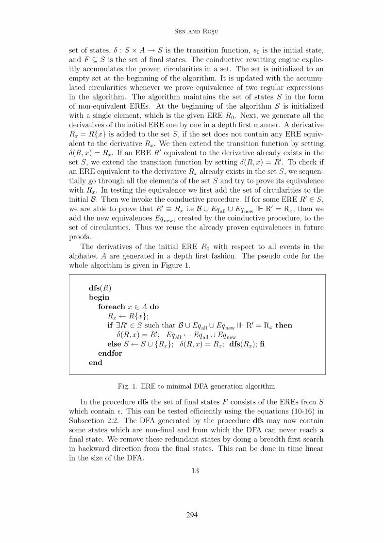
Sen and Rosu

set of states, δ : S × A → S is the transition function, s0 is the initial state,and F ⊆ S is the set of final states. The coinductive rewriting engine explic-itly accumulates the proven circularities in a set. The set is initialized to anempty set at the beginning of the algorithm. It is updated with the accumu-lated circularities whenever we prove equivalence of two regular expressionsin the algorithm. The algorithm maintains the set of states S in the formof non-equivalent EREs. At the beginning of the algorithm S is initializedwith a single element, which is the given ERE R0. Next, we generate all thederivatives of the initial ERE one by one in a depth first manner. A derivativeRx = Rx is added to the set S, if the set does not contain any ERE equiv-alent to the derivative Rx. We then extend the transition function by settingδ(R, x) = Rx. If an ERE R′ equivalent to the derivative already exists in theset S, we extend the transition function by setting δ(R, x) = R′. To check ifan ERE equivalent to the derivative Rx already exists in the set S, we sequen-tially go through all the elements of the set S and try to prove its equivalencewith Rx. In testing the equivalence we first add the set of circularities to theinitial B. Then we invoke the coinductive procedure. If for some ERE R′ ∈ S,we are able to prove that R′ ≡ Rx i.e B ∪ Eqall ∪ Eqnew ± R′ = Rx , then weadd the new equivalences Eqnew, created by the coinductive procedure, to theset of circularities. Thus we reuse the already proven equivalences in futureproofs.

The derivatives of the initial ERE R0 with respect to all events in thealphabet A are generated in a depth first fashion. The pseudo code for thewhole algorithm is given in Figure 1.

dfs(R)begin

foreach x ∈ A doRx ← Rx;if ∃R′ ∈ S such that B ∪ Eqall ∪ Eqnew ± R′ = Rx then

δ(R, x) = R′; Eqall ← Eqall ∪ Eqnew

else S ← S ∪ Rx; δ(R, x) = Rx; dfs(Rx); fiendfor

end

Fig. 1. ERE to minimal DFA generation algorithm

In the procedure dfs the set of final states F consists of the EREs from Swhich contain ε. This can be tested efficiently using the equations (10-16) inSubsection 2.2. The DFA generated by the procedure dfs may now containsome states which are non-final and from which the DFA can never reach afinal state. We remove these redundant states by doing a breadth first searchin backward direction from the final states. This can be done in time linearin the size of the DFA.

13

294

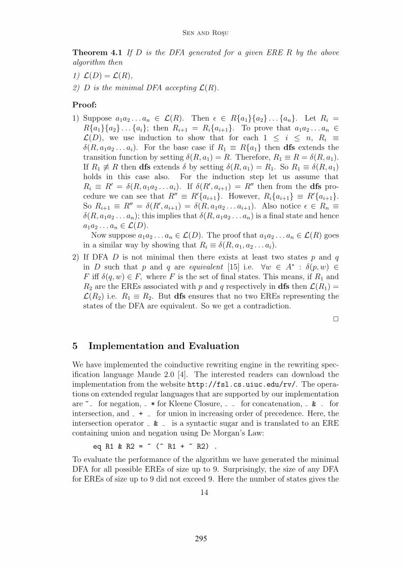
Sen and Rosu

Theorem 4.1 If D is the DFA generated for a given ERE R by the abovealgorithm then

1) L(D) = L(R),

2) D is the minimal DFA accepting L(R).

Proof:

1) Suppose a1a2 . . . an ∈ L(R). Then ε ∈ Ra1a2 . . . an. Let Ri =Ra1a2 . . . ai; then Ri+1 = Riai+1. To prove that a1a2 . . . an ∈L(D), we use induction to show that for each 1 ≤ i ≤ n, Ri ≡δ(R, a1a2 . . . ai). For the base case if R1 ≡ Ra1 then dfs extends thetransition function by setting δ(R, a1) = R. Therefore, R1 ≡ R = δ(R, a1).If R1 6≡ R then dfs extends δ by setting δ(R, a1) = R1. So R1 ≡ δ(R, a1)holds in this case also. For the induction step let us assume thatRi ≡ R′ = δ(R, a1a2 . . . ai). If δ(R′, ai+1) = R′′ then from the dfs pro-cedure we can see that R′′ ≡ R′ai+1. However, Riai+1 ≡ R′ai+1.So Ri+1 ≡ R′′ = δ(R′, ai+1) = δ(R, a1a2 . . . ai+1). Also notice ε ∈ Rn ≡δ(R, a1a2 . . . an); this implies that δ(R, a1a2 . . . an) is a final state and hencea1a2 . . . an ∈ L(D).

Now suppose a1a2 . . . an ∈ L(D). The proof that a1a2 . . . an ∈ L(R) goesin a similar way by showing that Ri ≡ δ(R, a1, a2 . . . ai).

2) If DFA D is not minimal then there exists at least two states p and qin D such that p and q are equivalent [15] i.e. ∀w ∈ A∗ : δ(p, w) ∈F iff δ(q, w) ∈ F, where F is the set of final states. This means, if R1 andR2 are the EREs associated with p and q respectively in dfs then L(R1) =L(R2) i.e. R1 ≡ R2. But dfs ensures that no two EREs representing thestates of the DFA are equivalent. So we get a contradiction.

2

5 Implementation and Evaluation

We have implemented the coinductive rewriting engine in the rewriting spec-ification language Maude 2.0 [4]. The interested readers can download theimplementation from the website http://fsl.cs.uiuc.edu/rv/. The opera-tions on extended regular languages that are supported by our implementationare ~ for negation, * for Kleene Closure, for concatenation, & forintersection, and + for union in increasing order of precedence. Here, theintersection operator & is a syntactic sugar and is translated to an EREcontaining union and negation using De Morgan’s Law:

eq R1 & R2 = ~ (~ R1 + ~ R2) .

To evaluate the performance of the algorithm we have generated the minimalDFA for all possible EREs of size up to 9. Surprisingly, the size of any DFAfor EREs of size up to 9 did not exceed 9. Here the number of states gives the

14

295

Sen and Rosu

size of a DFA. The following table shows the performance of our procedure forthe worst EREs of a given size. The code is executed on a Pentium 4 2.4GHz,4 GB RAM linux machine.

Size ERE no. of states in DFA Time (ms) Rewrites

4 ¬ (a b) 4 < 1 863

5 (a ¬ b) * 4 < 1 1370

6 ¬ ((a ¬ b) *) 4 1 1453

7 ¬ (a ¬ a a) 6 1 2261

8 ¬ ((a ¬ b) * b) 7 1 3778

9 ¬ (a ¬ a b) b 9 5 9717

Example 5.1 In particular, for the ERE ¬ (a ¬ a b) b the generated minimalDFA is given in Figure 2.

4

3

a

5b

6

b

a

7

b

8a

0

b

1

ab

2

a

b

a

b

aa

bb

a

Fig. 2. ¬ (a ¬ a b) b

Example 5.2 The ERE ¬ ((¬ empty) (green red) (¬ empty) ) states thesafety property that it should not be the case that in any trace of a trafficlight we see green and red consecutively at any point. The set of eventsare assumed to be green, red, yellow. We think that this is the mostintuitive and natural expression for this safety property. The implementationtook 1ms and 1663 rewrites to generate the minimal DFA with 2 states. TheDFA is given in Figure 3.

However for large EREs the algorithm may take a long time to generatea minimal DFA. The size of the generated DFA may grow non-elementarilyin the worst case. We generated DFAs for some complex EREs of larger sizesand got relatively promising results. One such sample result is as follows.

Example 5.3 Let us consider the following ERE of size 110

15

296

Sen and Rosu

0

red

yellow

1green

yellow

green

Fig. 3. ¬ ((¬ empty) (green red) (¬ empty))

(¬$)∗$(¬$)∗∩(0 + 1 + #)∗#(

((0 + 1)0#(0 + 1 + #)∗$(0 + 1)0 + (0 + 1)1#(0 + 1 + #)∗$(0 + 1)1)∩(0(0 + 1)#(0 + 1 + #)∗$0(0 + 1) + 1(0 + 1)#(0 + 1 + #)∗$1(0 + 1))).

This ERE accepts the language L2, where

Lk = σ#w#σ′$w | w ∈ 0, 1k and σ, σ′ ∈ 0, 1, #∗The language Lk was first introduced in [3] to show the power of alterna-

tion, used in [27] to show an exponential lower bound on ERE monitoring, andin [19,20] to show the lower bounds for model checking. Our implementationtook almost 18 minutes to generate the minimal DFA of size 107 and in theprocess it performed 1,374,089,220 rewrites.

The above example shows that the procedure can take a large amount oftime and space to generate DFAs for large EREs. To avoid the computationassociated with the generation of minimal DFA we plan to maintain a databaseof EREs and their corresponding minimal DFAs on the internet. Wheneversomeone wants to generate the minimal DFA for a given ERE he/she can lookup the internet database for the minimal DFA. If the ERE and the corre-sponding DFA exists in the database he/she can retrieve the correspondingDFA and use it as a monitor. Otherwise, he/she can generate the minimalDFA for the ERE and submit it to the internet database to create a new en-try. The database will check the equivalence of the submitted ERE and thecorresponding minimal DFA and insert it in the database. In this way onecan avoid the computation of generating minimal DFA if it is already done bysomeone else. To further reduce the computation, circularities could also bestored in the database.

5.1 Online Monitor Generation and Visualization

We have extended our implementation to create an internet server foroptimal monitor generation that can be accessed from the the urlhttp://fsl.cs.uiuc.edu/rv/. Given an ERE the server generates the opti-mal DFA monitor for a user. The user submits the ERE through a web based

16

297

Sen and Rosu

form. A CGI script handling the web form takes the submitted ERE as aninput, invokes the Maude implementation to generate the minimal DFA, andpresents it to the user either as a graphical or a textual representation. Togenerate the graphical representation of the DFA we are currently using theGraphViz tool [6].

6 Conclusion and Future Work

We presented a new technique to generate optimal monitors for extendedregular expressions, which avoids the traditional technique based on comple-mentation of automata, that we think is quite complex and not necessary.Instead, we have considered the (co)algebraic definition of EREs and appliedcoinductive inferencing techniques in an innovative way to generate the mini-mal DFA. Our approach to store already proven equivalences has resulted intoa very efficient and straightforward algorithm to generate minimal DFA. Wehave evaluated our implementation on several hundreds EREs and have gotpromising results in terms of running time. Finally, we have installed a serveron the internet which can generate the optimal DFA for a given ERE.

At least two major contributions have been made. Firstly, we have shownthat coinduction is a viable and quite practical method to prove equivalenceof extended regular expressions. Previously this was done only for regularexpressions without complementation. Secondly, building on the coinduc-tive technique, we have devised an algorithm to generate minimal DFAs fromEREs. At present we have no bound for the size of the optimal DFA, butwe know for sure that the DFAs we generate are indeed optimal. Howeverwe know that the size of an optimal DFA is bounded by some exponential inthe size of the ERE. As future work, it seems interesting to investigate thesize of minimal DFAs generated from EREs, and also to apply our coinductivetechniques to generate monitors for other logics, such as temporal logics.

References

[1] V. M. Antimirov. Partial derivatives of regular expressions and finite automatonconstructions. Theoretical Computer Science, 155(2):291–319, 1996.

[2] V. M. Antimirov and P. D. Mosses. Rewriting extended regular expressions.Theoretical Computer Science, 143(1):51–72, 1995.

[3] A. K. Chandra, D. C. Kozen, and L. J. Stockmeyer. Alternation. Journal ofthe ACM, 28(1):114–133, 1981.

[4] M. Clavel, F. Duran, S. Eker, P. Lincoln, N. Martı-Oliet, J. Meseguer, andJ. F. Quesada. Towards Maude 2.0. In 3rd International Workshop onRewriting Logic and its Applications (WRLA’00), volume 36 of Electronic Notesin Theoretical Computer Science. Elsevier, 2000.

17

298

Sen and Rosu

[5] D. Drusinsky. The Temporal Rover and the ATG Rover. In SPIN ModelChecking and Software Verification, volume 1885 of Lecture Notes in ComputerScience, pages 323–330. Springer, 2000.

[6] E. R. Gansner and S. C. North. An open graph visualization system andits applications to software engineering. Software Practice and Experience,30(1):1203–1233, September 2000.

[7] D. Giannakopoulou and K. Havelund. Automata-Based Verification ofTemporal Properties on Running Programs. In Proceedings, InternationalConference on Automated Software Engineering (ASE’01), pages 412–416.Institute of Electrical and Electronics Engineers, 2001. Coronado Island,California.

[8] J. Goguen, K. Lin, and G. Rosu. Circular coinductive rewriting. In Proceedings,Automated Software Engineering ’00, pages 123–131. IEEE, 2000. (Grenoble,France).

[9] J. Goguen, K. Lin, and G. Rosu. Conditional circular coinductive rewritingwith case analysis. In Recent Trends in Algebraic Development Techniques(WADT’02), Lecture Notes in Computer Science, to appear, Frauenchiemsee,Germany, September 2002. Springer-Verlag.

[10] K. Havelund and G. Rosu. Java PathExplorer – A Runtime Verification Tool.In The 6th International Symposium on Artificial Intelligence, Robotics andAutomation in Space: A New Space Odyssey, Montreal, Canada, June 18 - 21,2001.

[11] K. Havelund and G. Rosu. Monitoring Programs using Rewriting. InProceedings, International Conference on Automated Software Engineering(ASE’01), pages 135–143. Institute of Electrical and Electronics Engineers,2001. Coronado Island, California.

[12] K. Havelund and G. Rosu. Runtime Verification 2002, volume 70(4) ofElectronic Notes in Theoretical Computer Science. Elsevier Science, 2002.Proceedings of a Computer Aided Verification (CAV’02) satellite workshop.

[13] K. Havelund and G. Rosu. Synthesizing monitors for safety properties. In Toolsand Algorithms for Construction and Analysis of Systems (TACAS’02), volume2280 of Lecture Notes in Computer Science, pages 342–356. Springer, 2002.

[14] S. Hirst. A new algorithm solving membership of extended regular expressions.Technical report, The University of Sydney, 1989.

[15] J. E. Hopcroft and J. D. Ullman. Introduction to Automata Theory, Languagesand Computation. Addison Wesley, 1979.

[16] L. Ilie, B. Shan, and S. Yu. Fast algorithms for extended regular expressionmatching and searching. In H. Alt and M. Habib, editors, Proceedings of the20th International Symposium on Theoretical Aspects of Computer (STACS 03),volume 2607 of Lecture Notes in Computer Science, page 179. Springer-Verlag,Berlin, 2003.

18

299

Sen and Rosu

[17] M. Kim, S. Kannan, I. Lee, and O. Sokolsky. Java-MaC: a Run-time AssuranceTool for Java. In Proceedings of Runtime Verification (RV’01), volume 55 ofElectronic Notes in Theoretical Computer Science. Elsevier Science, 2001.

[18] J. Knight and E. Myers. Super-pattern matching. Algorithmica, 13(1/2):211–243, 1995.

[19] O. Kupferman and M. Y. Vardi. Freedom, Weakness, and Determinism: Fromlinear-time to branching-time. In Proceedings of the IEEE Symposium on Logicin Computer Science, pages 81–92, 1998.

[20] O. Kupferman and M. Y. Vardi. Model Checking of Safety Properties. InProceedings of the Conference on Computer-Aided Verification, 1999.

[21] O. Kupferman and S. Zuhovitzky. An Improved Algorithm for the MembershipProblem for Extended Regular Expressions. In Proceedings of the InternationalSymposium on Mathematical Foundations of Computer Science, 2002.

[22] I. Lee, S. Kannan, M. Kim, O. Sokolsky, and M. Viswanathan. RuntimeAssurance Based on Formal Specifications. In Proceedings of the InternationalConference on Parallel and Distributed Processing Techniques and Applications,1999.

[23] G. Myers. A four russians algorithm for regular expression pattern matching.Journal of the ACM, 39(4):430–448, 1992.

[24] T. O’Malley, D. Richardson, and L. Dillon. Efficient Specification-Based Oraclesfor Critical Systems. In In Proceedings of the California Software Symposium,1996.

[25] D. J. Richardson, S. L. Aha, and T. O. O’Malley. Specification-Based TestOracles for Reactive Systems. In Proceedings of the Fourteenth InternationalConference on Software Engineering, Melbourne, Australia, pages 105–118,1992.

[26] G. Rosu. Hidden Logic. PhD thesis, University of California at San Diego,2000.

[27] G. Rosu and M. Viswanathan. Testing extended regular language membershipincrementally by rewriting. In Rewriting Techniques and Applications(RTA’03), Lecture Notes in Computer Science, to appear. Springer-Verlag,2003.

[28] J. J. M. M. Rutten. Automata and coinduction (an exercise in coalgebra).In Proceedings of the 9th International Conference on Concurrency Theory(CONCUR 98), volume 1466 of Lecture Notes in Computer Science, pages 194–218. Springer-Verlag, 1998.

[29] K. Sen, G. Rosu, and G. Agha. Runtime safety analysis of multithreadedprograms. Technical Report UIUCDCS-R-2003-2334, University of Illinois atUrnaba Champaign, April 2003.

19

300

Sen and Rosu

[30] B. Watson. A taxonomy of deterministic finite automata minimizationalgorithms. Technical Report ISSN 0926-4515, Eindhoven University ofTechnology, Eindhoven, The Netherlands, 1993.

[31] H. Yamamoto. An automata-based recognition algorithm for semi-extendedregular expressions. In Proceedings of the International Symposium onMathematical Foundations of Computer Science, pages 699–708, 2000.

20

301

! "##

Æ Æ !

! " #$ % & ! '

(

" # ' $ ( # $ ! # $ # $

) *

+

302

! , " %!& "

- . # /0 12 /312 /452$ " ,

. " .

. 6 " "

' " 4 % & 7 8#$ 4 4 ! #$ #$ 8#$ 4 1! ! 4 Æ

# $ ! ' % & 9 % & # /752$

(

!

:

303

#$ ; ! < * ! (

= ( , /1)2 " />-2

" > = - #$ " Æ # $ " /752

" 4 ( # $ (

? 6 ! (

$# % &'

> . @ /A>32 ! " ( = ! (

#$ #$ ! ! " "

" #$ !% & & &

& ! & & ' & '

() !

B

304

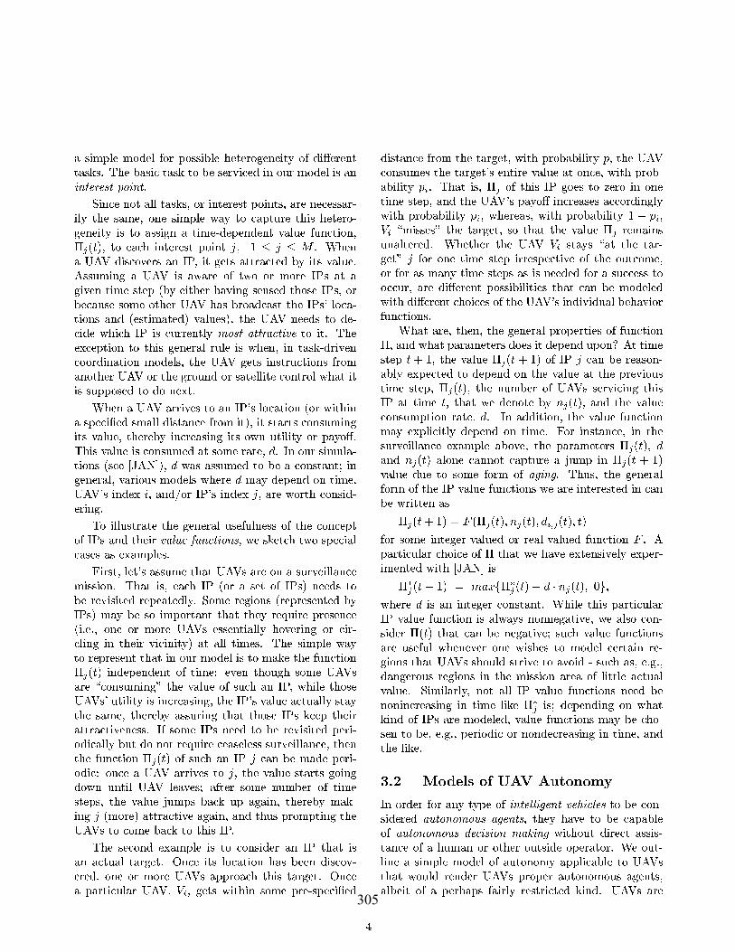
9

- 8#$ + " 4 4 # 4 4( #$ $ 4

" 4( # $ 9 # /C)2$ * ( ' 4(

4

= ( 4 # 4$ - # 4$ ! # $ 8#$ 6 %& 4 ( 4( 4 4 ! 8#$ 4 6 * < # $ 4

4 > >

( 8 4 ( 9 + %& 8 " % & 9 9 (

" 8 D E + 8# E +$ 4 8#$ 4 #$ = 8#$ #$ < 8# E +$ 4

8#E +$ F #8#$ #$ #$ $

8 /C)2

8 #E +$ F 8

#$ #$ G

" 4 8#$ * - 4 8

* 4

$#! % &'

"

H

305

( 4 ! 6 4 4D = #$ 4 D

" ( ( ; I 4 ; 4 4 ( , 9 ;

- ( 4 4( # $ 4 4( 5 #$ 4 4 (

;#$ F #8 $

8 4 #$ #$ 4 ) >

;#$ F /

2

4

7 ( # ; $ > ( ;#$ #$ #$ "

$#$ % &'

"

% & 4 # $ # $ 9 ( ' # $

" 9 > ! % & # $ %< & % &

* & !+ , & (

" (( !

J

306

% & %

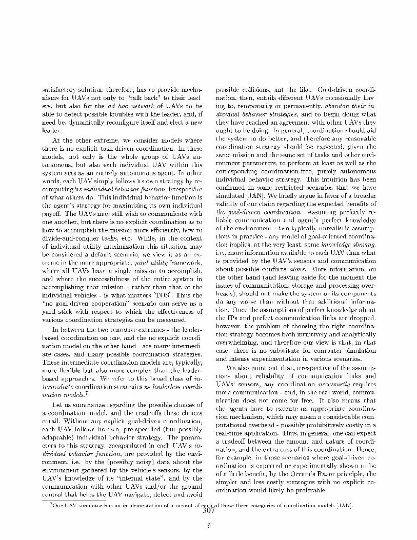
( 9 Æ ! " ! />-2 % & 9

. "

5 9 " # $ ( # $ ( ( % & '

I 9 /C)2 " . ( % ( . @ # $ > 4

" ( ! 9 , >( K

- #$ !

L

307

! "

" K ( 9 4 4 6 4

4 8 ( # <$ 4 4 4( & % ( 8 4 ' ( ; ! ; 4 8 /4K2

# "

" 9 9

" ! "!#$ #% ! &'('''')(

'

/0 12 0 5 4 &> . Æ & 777 - + ? :GGG

/1)2 ? , 1 & 1 - = ? 4 " 4 & 4? 1 +MNJ

/=K2 - = I % < 4 D & 4 B ( " O 5 - +MML

/C)2 @ C - K 4 5 1I % - @ 1 & +J7 - - O 7 ? ) :GGB

/312 C 3 3 5 1 A & . & 777 - +? :GGG

/452 5 4 7 @ = 0 &1. K 4 Æ @- - " @ 4 & 777 - B) + @ :GG:

/4K2 - 4 @ " %I ? @ -& @- ) J :GG: 3 4

/752 I & ? & : 1 4 :GGG

/>-2 4 @ C I %1 > = - @ 4 &

/A>32 @ A 3 , % ? 1 -6 & @- B ) : :GGG

P

308

Runtime Safety Analysis of Multithreaded Programs

Koushik Sen∗

Dept. of Computer ScienceUniversity of Illinois at Urbana

ksen@uiuc.edu

Grigore Rosu†

Dept. of Computer ScienceUniversity of Illinois at Urbana

grosu@uiuc.edu

Gul Agha‡

Dept. of Computer ScienceUniversity of Illinois at Urbana

agha@uiuc.edu

ABSTRACTFoundational and scalable techniques for runtime safetyanalysis of multithreaded programs are explored in this pa-per. A technique based on vector clocks to extract the causaldependency order on state updates from a running multi-threaded program is presented, together with algorithms toanalyze a multithreaded computation against safety prop-erties expressed using temporal logics. A prototype toolimplementing our techniques, is also presented, togetherwith examples where it can predict safety errors in multi-threaded programs from successful executions of those pro-grams. This tool is called Java MultiPathExplorer (JM-PaX), and available for download on the web. To the bestof our knowledge, JMPaX is the first tool of its kind.

Categories and Subject DescriptorsD.2.4 [Software Engineering]: Software/Program Verifi-cation

General TermsVerification

KeywordsLTL, predictive analysis, safety analysis, runtime monitor-ing, vector clock, multithreaded program, JMPaX, Java

∗Supported in part by the Defense Advanced ResearchProjects Agency (Contract numbers: F30602-00-2-0586 andF33615-01-C-1907) and the ONR Grant N00014-02-1-0715.†Supported in part by joint NSF/NASA grant CCR-0234524‡Supported in part by the Defense Advanced ResearchProjects Agency (Contract numbers: F30602-00-2-0586 andF33615-01-C-1907) and the ONR Grant N00014-02-1-0715.

Permission to make digital or hard copies of all or part of this work forpersonal or classroom use is granted without fee provided that copies arenot made or distributed for profit or commercial advantage and that copiesbear this notice and the full citation on the first page. To copy otherwise, torepublish, to post on servers or to redistribute to lists, requires prior specificpermission and/or a fee.ESEC/FSE’03,September 1–5, 2003, Helsinki, Finland.Copyright 2003 ACM 1-58113-743-5/03/0009 ...$5.00.

1. INTRODUCTIONThe purpose of this paper is to investigate foundational,

scalable techniques for runtime safety analysis of multi-threaded programs, i.e., programs in which several executionthreads communicate with each other via shared variablesand synchronization points, as well as to introduce a pro-totype tool, called Java MultiPathExplorer (JMPaX – seeFigure 1), based on our foundational techniques, which canreveal errors in multithreaded programs that are hard orimpossible to detect otherwise. The user of JMPaX spec-ifies safety properties of interest, using a past time tem-poral logic, regarding the global state of a multithreadedprogram, which is already assumed in compiled form, callsan instrumentation script which automatically instrumentsthe executable multithreaded program to emit relevant stateupdate events to an external observer, and finally runs theprogram on any JVM and analyzes the safety violation mes-sages reported by the observer. A particularly appealingaspect of our approach is that, despite the fact that a sin-gle execution, or interleaving, of a multithreaded programcan be observed, a comprehensive analysis of all possibleexecutions is performed; a possible execution is any execu-tion which does not violate the observed causal dependencypartial order on state update events. Thus, tools built onour techniques, including JMPaX, have the ability to pre-dict safety violation errors in multithreaded programs byobserving successful executions.

The work in this paper falls under the area recently calledruntime verification [11, 10], a major goal of which is tocombine testing and formal methods techniques. Testingscales well, and is by far the most used technique in prac-tice to validate software systems. By merging testing andtemporal logic specification, we aim to achieve the bene-fits of both approaches, while avoiding some of the pitfallsof ad hoc testing and the complexity of full-blown theoremproving and model checking. Of course, there is a price tobe paid in order to obtain a scalable technique: the lossof coverage. The suggested framework can only be used toexamine single execution traces, and therefore can not beused to prove a system correct. However, a single execu-tion trace typically contains much more information thanwhat appears at first sight. In this paper, we show how onecan analyze all the other multithreaded executions that arehidden behind a particular observed execution. Our workis based on the belief that software engineers are willing totrade coverage for scalability, so our goals are to providetools that use formal methods techniques in a lightweightmanner, use unmodified programming languages or under-

309

Specification

Java

Multithreaded

Program

Bytecode

Compile

Instrumentor

Instrumented

Bytecode

Translator

SpecificationImpl

LTL Monitor

Execute

Level 0

Level 5

Level 4

Level 3

Level 2

Level 1

Computation Lattice

Monitor

Execution Program Execution

JVM

Instrument

Event Stream

Instrumentation

Module Monitoring

Module

Figure 1: JMPaX Architecture

lying executional engines (such as JVMs), are completelyautomatic, implement very efficient algorithms and eventu-ally find many errors in programs. A longer term goal is toexplore the use of conformance with a formal specificationto achieve error recovery. The idea is that a predicted fail-ure may trigger an error-avoidance or recovery action in themonitored program.

The closest works in spirit to ours are NASA’s PathEx-plorer (PaX) and its Java instance JPaX [10, 9], which is aruntime verification system developed at NASA Ames, andUPENN’s MaC and its instance Java MaC [14, 15]. It isactually the latter’s limitations that motivated us to pursueour current research. The major limitation of these systemswith regards to safety analysis is that they only analyze theobserved run. Therefore, they can only detect existing er-rors in current executions; they do not have the ability topredict possible errors from successful runs. To be more pre-cise in our claim, let us consider a real-life example whereJMPaX was able to detect a violation of a safety propertyfrom a single execution of the program. However, the likeli-hood of detecting this bug only by monitoring the observedrun, as JPaX and Java-MAC do, is very low. The exampleconsists of a two threaded program to control the landing ofan airplane. It has three variables landing, approved, andradio; their values are 1 when the plane is landing, landinghas been approved, and radio signal is live, and 0 otherwise.The safety property that we want to verify is “If the planehas started landing, then it is the case that landing has beenapproved and since the approval the radio signal has neverbeen down.” As shown in Subsection 3.1, this property canbe formally written in our extension of past time linear tem-poral logic as the formula

↑landing→ [approved, ↓radio)s.

The code snippet for a naive implementation of this controlprogram is given as follows:

int landing = 0, approved = 0, radio = 1;void thread1()

askLandingApproval();if(approved==1)

print("Landing approved");landing = 1;print("Landing started");

else print("Landing not approved");

void askLandingApproval()if(radio==0) approved = 0;else approved = 1;

void thread2()while(radio)checkRadio();

void checkRadio()randomly change value of radio;

The above code uses some dummy functions, namelyaskLandingApproval and checkRadio, which can be imple-mented in their entirety in a real scenario. The programhas a serious problem which cannot be detected easily froma single run. The problem is as follows. Suppose the planehas received approval for landing and just before it startedlanding the radio signal went off. In this situation, the planemust abort landing. But this situation will very rarely arisein an execution: namely, when radio is set to 0 between theapproval of landing and the start of actual landing. So asimple observer will not probably detect the bug. However,note that even if the radio goes off after the landing hasstarted, JMPaX can still construct a possible run in whichradio goes off between landing and approval. Thus JMPaXwill be able to predict the safety violation from a single suc-cessful execution of the program. This example shows thepower of our runtime verification technique as compared toJPaX and Java-MaC.

Other related approaches include model checking [6], es-pecially Java bytecode model checking [8], and debuggingof distributed systems. It is important to observe that, un-like model checking where all possible code interleavings areanalyzed, in our approach to runtime safety analysis oneactually runs the program and extracts causal dependen-cies among updates of the multithreaded program state, andthen analyzes all possible interleavings that do not violatethe causal dependency. At the expense of a lower coverage,our approach analyzes a significantly lower amount of threadinterleavings than a typical model checker would normallydo, so it scales up better. The safety properties that weanalyze are more general than the simpler state predicatesthat are typically considered in the literature on debuggingdistributed systems (see for example [19, 4, 3]). We allowany past time linear temporal logic formula built on statepredicates, so our safety properties can refer to the entirepast history of states. An important practical aspect of ouralgorithm is that, despite the fact that there can be a po-tentially exponential number of runs (in the length of theruns), they can all be analyzed in parallel, by generatingand traversing the computation lattice extracted from the

310

observed multithreaded execution on a level-by-level basis.The relevant information regarding the previous levels canbe encoded compactly, so those levels do not need to bestored, thus allowing the memory to be reused.

We can think of at least three major contributions of thework presented in this paper. First, we nontrivially extendthe runtime safety analysis capabilities of systems like JPaXand Java Mac, by providing the ability to predict safety er-rors from successful executions; we are not aware of anyother efforts in this direction. Second, we underlie the foun-dations of relevant causality in multithreaded systems withshared variables and synchronization points, which one canuse to instrument multithreaded programs to emit to exter-nal observers a causal dependency partial relation on globalstate updates via relevant events timestamped with appro-priate vector clocks; this is done in Section 2, where, due toits foundational aspect, all the proofs of the claimed resultsare provided. Finally, a modular implementation of a pro-totype runtime analysis system, JMPaX, is given, showingthat, despite their theoretical flavor, all the concepts pre-sented in the paper are in fact quite practical and can leadto new scalable verification tools.

2. RELEVANT CAUSALITY INMULTITHREADED SYSTEMS

We consider multithreaded systems in which severalthreads communicate with each other via a set of sharedvariables. The theme of this paper is to show how such asystem can be analyzed for safety by an external observerthat obtains relevant information about the system frommessages sent by the system after appropriate instrumenta-tion. The safety formulae refer to sets of shared variables,so these messages contain update information about thosevariables. A crucial observation here is that some variableupdates can causally depend on others. For example, if athread writes a variable x and then another thread writes ydue to a statement y = x + 1, then the update of y causallydepends upon the update of x. In this section we present analgorithm which, given an executing multithreaded system,generates appropriate messages to be sent to an externalobserver. The observer, in order to perform its more elabo-rated safety analysis, extracts the state update informationfrom such messages together with the causality partial orderorder among the updates.

Formally, given n threads p1, p2, ..., pn, a multithreadedexecution is abstracted as a sequence of events e1e2 . . . er,each belonging to one of the n threads and being of type ei-ther internal or read or write of a shared variable. We use ej

i

to represent the j-th event generated by thread pi since thestart of its execution. From now on in this section we assumean arbitrary but fixed multithreaded execution. When theprocess or the position of an event is not important then wecan refer to the event generically, such as e, e′, etc.; we maywrite e ∈ pi when event e is generated by thread pi. Let Sbe the set of shared variables. There is an immediate notionof variable access precedence for each shared variable x ∈ S:we say that e x-precedes e′, written e <x e′, if and only ife and e′ are variable access events (reads or writes) to thesame variable x, and e “happens before” e′; this “happen-before” relation can be easily realized by keeping a counterfor each shared variable which is increased by each accessto it. Let E be the set of all the events of a multithreaded

execution, and let ≺ be the partial order on E defined asfollows:

• eki ≺ el

i if k < l;

• e ≺ e′ if there is some x ∈ S such that e <x e′ andatleast one of e, e′ is a write.

• e ≺ e′′ if e ≺ e′ and e′ ≺ e′′.

We write e||e′ when it is not the case that e ≺ e′ ore′ ≺ e. A partial order on events ≺ defined above iscalled a multithreaded computation associated with the orig-inal multithreaded execution. As shown in Subsection 3.3,synchronization can be treated very elegantly by generatingappropriate read/write events, so that the notion of mul-tithreaded computation as defined above is as general ascurrently needed. Note that the original multithreaded ex-ecution was used only to provide a total ordering on theread/write accesses of each shared variable.1 A permuta-tion of all the events e1, e2, ..., er which does not violatethe multithreaded computation is called a consistent multi-threaded run, or simply, a multithreaded run.

Intuitively, e ≺ e′, read as e′ causally depends upon e, ifand only if e occurred before e′ in the given multithreadedexecution and a change of their order does not generate aconsistent multithreaded run. We argue that the notion ofmultithreaded computation defined above is the weakest as-sumption that an omniscient observer of the multithreadedexecution can make about the program. Intuitively, this isbecause an external observer cannot disregard the order inwhich the same variable is modified and used within theobserved execution, because this order can be part of theintrinsic logic of the multithreaded program. However, mul-tiple consecutive reads of the same variable can be permuted,and the particular order observed in the given execution isnot critical; it can be, for example, a result of a particu-lar thread scheduling algorithm. By allowing an observer toanalyze multithreaded computations rather than just multi-threaded run, one gets the benefit of not only properly deal-ing with potential reordering of delivered messages (for ex-ample, due to using multiple channels in order to reduce themonitoring overhead), but also of predicting errors from an-alyzing successful executions, errors which can occur undera different thread scheduling.

Not all the variable in S are needed to evaluate the safetyformula to be checked. To minimize number of messagessent to an observer, and for technical reasons discussed later,we consider a subset R ⊆ E of relevant events. Then wedefine the R-relevant causality on E as the relation / :=≺∩(R×R), so that e / e′ if and only if e, e′ ∈ R and e ≺ e′.We provide a technique based on vector clocks [7, 17] thatcorrectly implements the relevant causality relation.

Let Vi be an n-dimensional vector of natural numbers forthread pi, for each 1 ≤ i ≤ n, and let V a

x and V wx be two

additional n-dimensional vectors for each shared variable x;we call the former access vector clock and the latter writevector clock. All the vector clocks are initialized to 0 at thebeginning of computation. For two n-dimensional vectors wesay that V ≤ V ′ if and only if V [j] ≤ V ′[j] for all 1 ≤ j ≤ n,and we say that V < V ′ iff V ≤ V ′ and there is some1 ≤ j ≤ n such that V [j] < V ′[j]; also, maxV, V ′ is

1One could have defined a multithreaded computation moreabstractly but less intuitively, by starting with a total order<x on the subset of events accessing each shared variable x.

311

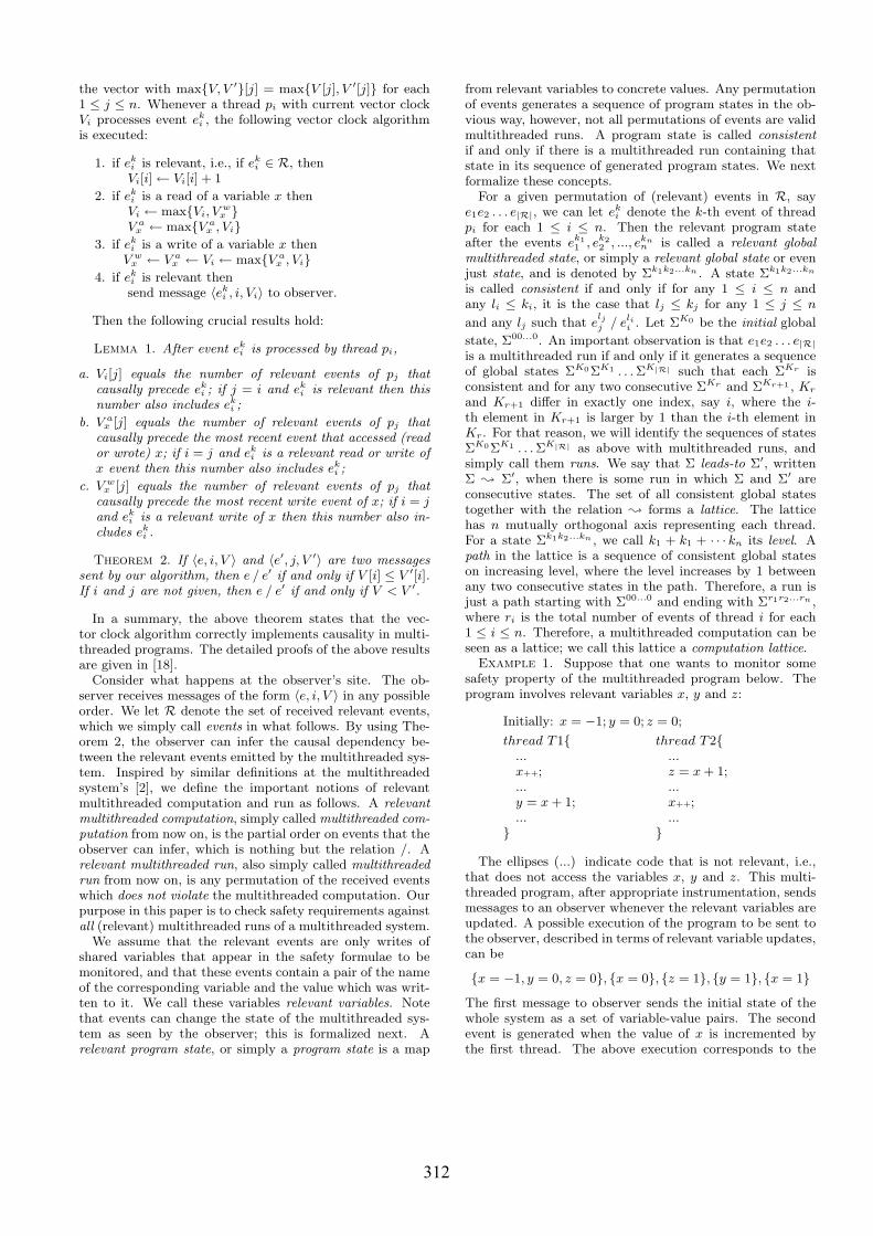
the vector with maxV, V ′[j] = maxV [j], V ′[j] for each1 ≤ j ≤ n. Whenever a thread pi with current vector clockVi processes event ek

i , the following vector clock algorithmis executed:

1. if eki is relevant, i.e., if ek

i ∈ R, thenVi[i] ← Vi[i] + 1

2. if eki is a read of a variable x thenVi ← maxVi, V

wx

V ax ← maxV a

x , Vi3. if ek

i is a write of a variable x thenV w

x ← V ax ← Vi ← maxV a

x , Vi4. if ek

i is relevant thensend message 〈ek

i , i, Vi〉 to observer.

Then the following crucial results hold:

Lemma 1. After event eki is processed by thread pi,

a. Vi[j] equals the number of relevant events of pj thatcausally precede ek

i ; if j = i and eki is relevant then this

number also includes eki ;

b. V ax [j] equals the number of relevant events of pj that

causally precede the most recent event that accessed (reador wrote) x; if i = j and ek

i is a relevant read or write ofx event then this number also includes ek

i ;

c. V wx [j] equals the number of relevant events of pj that

causally precede the most recent write event of x; if i = jand ek

i is a relevant write of x then this number also in-cludes ek

i .

Theorem 2. If 〈e, i, V 〉 and 〈e′, j, V ′〉 are two messagessent by our algorithm, then e / e′ if and only if V [i] ≤ V ′[i].If i and j are not given, then e / e′ if and only if V < V ′.

In a summary, the above theorem states that the vec-tor clock algorithm correctly implements causality in multi-threaded programs. The detailed proofs of the above resultsare given in [18].

Consider what happens at the observer’s site. The ob-server receives messages of the form 〈e, i, V 〉 in any possibleorder. We let R denote the set of received relevant events,which we simply call events in what follows. By using The-orem 2, the observer can infer the causal dependency be-tween the relevant events emitted by the multithreaded sys-tem. Inspired by similar definitions at the multithreadedsystem’s [2], we define the important notions of relevantmultithreaded computation and run as follows. A relevantmultithreaded computation, simply called multithreaded com-putation from now on, is the partial order on events that theobserver can infer, which is nothing but the relation /. Arelevant multithreaded run, also simply called multithreadedrun from now on, is any permutation of the received eventswhich does not violate the multithreaded computation. Ourpurpose in this paper is to check safety requirements againstall (relevant) multithreaded runs of a multithreaded system.

We assume that the relevant events are only writes ofshared variables that appear in the safety formulae to bemonitored, and that these events contain a pair of the nameof the corresponding variable and the value which was writ-ten to it. We call these variables relevant variables. Notethat events can change the state of the multithreaded sys-tem as seen by the observer; this is formalized next. Arelevant program state, or simply a program state is a map

from relevant variables to concrete values. Any permutationof events generates a sequence of program states in the ob-vious way, however, not all permutations of events are validmultithreaded runs. A program state is called consistentif and only if there is a multithreaded run containing thatstate in its sequence of generated program states. We nextformalize these concepts.

For a given permutation of (relevant) events in R, saye1e2 . . . e|R|, we can let ek

i denote the k-th event of threadpi for each 1 ≤ i ≤ n. Then the relevant program stateafter the events ek1

1 , ek22 , ..., ekn

n is called a relevant globalmultithreaded state, or simply a relevant global state or evenjust state, and is denoted by Σk1k2...kn . A state Σk1k2...kn

is called consistent if and only if for any 1 ≤ i ≤ n andany li ≤ ki, it is the case that lj ≤ kj for any 1 ≤ j ≤ n

and any lj such that eljj / eli

i . Let ΣK0 be the initial global

state, Σ00...0. An important observation is that e1e2 . . . e|R|is a multithreaded run if and only if it generates a sequenceof global states ΣK0ΣK1 . . . ΣK|R| such that each ΣKr isconsistent and for any two consecutive ΣKr and ΣKr+1 , Kr

and Kr+1 differ in exactly one index, say i, where the i-th element in Kr+1 is larger by 1 than the i-th element inKr. For that reason, we will identify the sequences of statesΣK0ΣK1 . . . ΣK|R| as above with multithreaded runs, andsimply call them runs. We say that Σ leads-to Σ′, writtenΣ ; Σ′, when there is some run in which Σ and Σ′ areconsecutive states. The set of all consistent global statestogether with the relation ; forms a lattice. The latticehas n mutually orthogonal axis representing each thread.For a state Σk1k2...kn , we call k1 + k1 + · · · kn its level. Apath in the lattice is a sequence of consistent global stateson increasing level, where the level increases by 1 betweenany two consecutive states in the path. Therefore, a run isjust a path starting with Σ00...0 and ending with Σr1r2...rn ,where ri is the total number of events of thread i for each1 ≤ i ≤ n. Therefore, a multithreaded computation can beseen as a lattice; we call this lattice a computation lattice.

Example 1. Suppose that one wants to monitor somesafety property of the multithreaded program below. Theprogram involves relevant variables x, y and z:

Initially: x = −1; y = 0; z = 0;

thread T1...x++;...y = x + 1;...

thread T2...z = x + 1;...x++;...

The ellipses (...) indicate code that is not relevant, i.e.,that does not access the variables x, y and z. This multi-threaded program, after appropriate instrumentation, sendsmessages to an observer whenever the relevant variables areupdated. A possible execution of the program to be sent tothe observer, described in terms of relevant variable updates,can be

x = −1, y = 0, z = 0, x = 0, z = 1, y = 1, x = 1The first message to observer sends the initial state of thewhole system as a set of variable-value pairs. The secondevent is generated when the value of x is incremented bythe first thread. The above execution corresponds to the

312

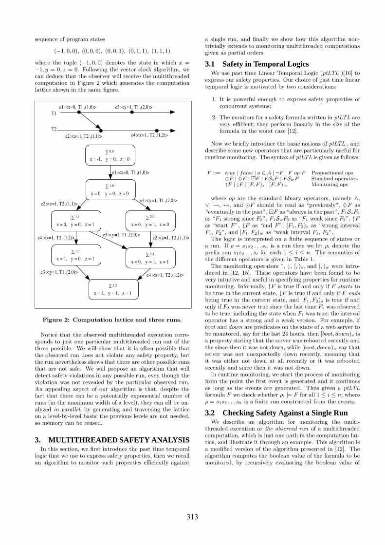
sequence of program states

(−1, 0, 0), (0, 0, 0), (0, 0, 1), (0, 1, 1), (1, 1, 1)

where the tuple (−1, 0, 0) denotes the state in which x =−1, y = 0, z = 0. Following the vector clock algorithm, wecan deduce that the observer will receive the multithreadedcomputation in Figure 2 which generates the computationlattice shown in the same figure.

S 0 ,0

x = -1, y = 0, z = 0

S 2 ,2

x = 1, y = 1, z = 1

S 2 ,1

x = 0, y = 1, z = 1

S 2 ,0

x = 0, y = 1, z = 0

S 1 ,1

x = 0, y = 0, z = 1

S 1 ,0

x = 0, y = 0, z = 0

e1 :<x=0, T1 ,(1,0)>

e4 :<x=1, T2 ,(1,2)>

e2 :< z =1, T2 ,(1,1)> e3 :< y =1, T1 ,(2,0)>

e2 :< z =1, T2 ,(1,1)> e3 :< y =1, T1 ,(2,0)>

e1 :<x=0, T1 ,(1,0)>

e2 :< z =1, T2 ,(1,1)>

e3 :< y =1, T1 ,(2,0)>

e4 :<x=1, T2 ,(1,2)>

T1

T2

S 1 ,2

x = 1, y = 0, z = 1

e4 :<x=1, T2 ,(1,2)>

e3 :< y =1, T1 ,(2,0)>

Figure 2: Computation lattice and three runs.

Notice that the observed multithreaded execution corre-sponds to just one particular multithreaded run out of thethree possible. We will show that it is often possible thatthe observed run does not violate any safety property, butthe run nevertheless shows that there are other possible runsthat are not safe. We will propose an algorithm that willdetect safety violations in any possible run, even though theviolation was not revealed by the particular observed run.An appealing aspect of our algorithm is that, despite thefact that there can be a potentially exponential number ofruns (in the maximum width of a level), they can all be an-alyzed in parallel, by generating and traversing the latticeon a level-by-level basis; the previous levels are not needed,so memory can be reused.

3. MULTITHREADED SAFETY ANALYSISIn this section, we first introduce the past time temporal

logic that we use to express safety properties, then we recallan algorithm to monitor such properties efficiently against

a single run, and finally we show how this algorithm non-trivially extends to monitoring multithreaded computationsgiven as partial orders.

3.1 Safety in Temporal LogicsWe use past time Linear Temporal Logic (ptLTL )[16] to

express our safety properties. Our choice of past time lineartemporal logic is motivated by two considerations:

1. It is powerful enough to express safety properties ofconcurrent systems;

2. The monitors for a safety formula written in ptLTL arevery efficient; they perform linearly in the size of theformula in the worst case [12].

Now we briefly introduce the basic notions of ptLTL , anddescribe some new operators that are particularly useful forruntime monitoring. The syntax of ptLTL is given as follows:

F ::= true | false | a ∈ A | ¬F | F op F Propositional ops¯F | ♦· F | ¡F | FSsF | FSwF Standard operators↑F | ↓F | [F, F )s | [F, F )w Monitoring ops

where op are the standard binary operators, namely ∧,∨, →, ↔, and ¯F should be read as “previously”, ♦· F as“eventually in the past”, ¡F as “always in the past”, F1SsF2

as “F1 strong since F2”, F1SwF2 as “F1 weak since F2”, ↑Fas “start F”, ↓F as “end F”, [F1, F2)s as “strong intervalF1, F2”, and [F1, F2)w as “weak interval F1, F2”.

The logic is interpreted on a finite sequence of states ora run. If ρ = s1s2 . . . sn is a run then we let ρi denote theprefix run s1s2 . . . si for each 1 ≤ i ≤ n. The semantics ofthe different operators is given in Table 1.

The monitoring operators ↑, ↓, [, )s, and [, )w were intro-duced in [12, 15]. These operators have been found to bevery intuitive and useful in specifying properties for runtimemonitoring. Informally, ↑F is true if and only if F starts tobe true in the current state, ↓F is true if and only if F endsbeing true in the current state, and [F1, F2)s is true if andonly if F2 was never true since the last time F1 was observedto be true, including the state when F1 was true; the intervaloperator has a strong and a weak version. For example, ifboot and down are predicates on the state of a web server tobe monitored, say for the last 24 hours, then [boot, down)s isa property stating that the server was rebooted recently andthe since then it was not down, while [boot, down)w say thatserver was not unexpectedly down recently, meaning thatit was either not down at all recently or it was rebootedrecently and since then it was not down.

In runtime monitoring, we start the process of monitoringfrom the point the first event is generated and it continuesas long as the events are generated. Thus given a ptLTLformula F we check whether ρi |= F for all 1 ≤ i ≤ n, whereρ = s1s2 . . . sn is a finite run constructed from the events.

3.2 Checking Safety Against a Single RunWe describe an algorithm for monitoring the multi-

threaded execution or the observed run of a multithreadedcomputation, which is just one path in the computation lat-tice, and illustrate it through an example. This algorithm isa modified version of the algorithm presented in [12]. Thealgorithm computes the boolean value of the formula to bemonitored, by recursively evaluating the boolean value of

313

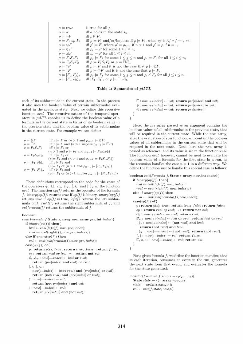
ρ |= true is true for all ρ,ρ |= a iff a holds in the state sn,ρ |= ¬F iff ρ 2 F ,ρ |= F1 op F2 iff ρ |= F1 and/or/implies/iff ρ |= F2, when op is ∧/ ∨ / → / ↔,ρ |= ¯F iff ρ′ |= F , where ρ′ = ρn−1 if n > 1 and ρ′ = ρ if n = 1,ρ |= ♦· F iff ρi |= F for some 1 ≤ i ≤ n,ρ |= ¡F iff ρi |= F for all 1 ≤ i ≤ n,ρ |= F1SsF2 iff ρj |= F2 for some 1 ≤ j ≤ n and ρi |= F1 for all 1 ≤ i ≤ n,ρ |= F1SwF2 iff ρ |= F1SsF2 or ρ |= ¡F1,ρ |= ↑F iff ρ |= F and it is not the case that ρ |= ¯F ,ρ |= ↓F iff ρ |= ¯F and it is not the case that ρ |= F ,ρ |= [F1, F2)s iff ρj |= F1 for some 1 ≤ j ≤ n and ρi 2 F2 for all j ≤ i ≤ n,ρ |= [F1, F2)w iff [F1, F2)s or ρ |= ¡¬F2,

Table 1: Semantics of ptLTL

each of its subformulae in the current state. In the processit also uses the boolean value of certain subformulae eval-uated in the previous state. Next we define this recursivefunction eval. The recursive nature of the temporal oper-ators in ptLTL enables us to define the boolean value of aformula in the current state in terms of its boolean value inthe previous state and the boolean value of its subformulaein the current state. For example we can define:

ρ |= ♦· F iff ρ |= F or (n > 1 and ρn−1 |= ♦· F )ρ |= ¡F iff ρ |= F and (n > 1 implies ρn−1 |= ¡F )ρ |= F1SsF2 iff ρ |= F2 or

(n > 1 and ρ |= F1 and ρn−1 |= F1SsF2)ρ |= F1SwF2 iff ρ |= F2 or

(ρ |= F1 and (n > 1 and ρn−1 |= F1SwF2))ρ |= [F1, F2)s iff ρ 2 F2 and

(ρ |= F1 or (n > 1 and ρn−1 |= [F1, F2)s))ρ |= [F1, F2)w iff ρ 2 F2 and

(ρ |= F1 or (n > 1 implies ρn−1 |= [F1, F2)w))

These definitions correspond to the code for the cases ofthe operators ♦· , ¡, Ss, Sw, [, )s, and [, )w in the functioneval. The function op(f) returns the operator of the formulaf , binary(op(f)) returns true if op(f) is binary, unary(op(f))returns true if op(f) is true, left(f) returns the left subfor-mula of f , right(f) returns the right subformula of f , andsubformula(f) returns the subformula of f .

boolean

eval(Formula f,State s,array now,array pre, int index)if binary(op(f)) then

lval ← eval(left(f), now, pre, index);

rval ← eval(right(f), now, pre, index); else if unary(op(f)) then

val ← eval(subformula(f), now, pre, index);

case(op(f)) ofp : return p(s); true : return true; false : return false;

op : return rval op lval; ¬ : return not val;

Ss,Sw : now[++index] ← lval or rval;

return (pre[index] and lval) or rval;

[, )s, [, )w :

now[++index] ← (not rval) and (pre[index] or lval);

return (not rval) and (pre[index] or lval);

↑ : now[++index] ← val;

return (not pre[index]) and val;

↓ : now[++index] ← val;

return pre[index] and (not val);

¡ : now[++index] ← val; return pre[index] and val;

♦· : now[++index] ← val; return pre[index] or val;

¯ : now[++index] ← val; return pre[index];

Here, the pre array passed as an argument contains theboolean values of all subformulae in the previous state, thatwill be required in the current state. While the now array,after the evaluation of eval function, will contain the booleanvalues of all subformulae in the current state that will berequired in the next state. Note, here the now array ispassed as reference, and its value is set in the function eval.The function eval, however, cannot be used to evaluate theboolean value of a formula for the first state in a run, asthe recursion handles the case n = 1 in a different way. Wedefine the function init to handle this special case as follows:

boolean init(Formula f,State s,array now, int index)if binary(op(f)) then

lval ← init(left(f), now, index);

rval ← eval(right(f), now, index); else if unary(op(f)) then

val ← init(subformula(f), now, index);

case(op(f)) ofp : return p(s); true : return true; false : return false;

op : return rval op lval; ¬ : return not val;

Ss : now[++index] ← rval; return rval;

Sw : now[++index] ← lval or rval; return lval or rval;

[, )s : now[++index] ← (not rval) and lval;

return (not rval) and lval;

[, )w : now[++index] ← (not rval); return (not rval);

↑, ↓ : now[++index] ← val; return false;

¡, ♦· ,¯ : now[++index] ← val; return val;

For a given formula f , we define the function monitor, thatat each iteration, consumes an event in the run, generatesthe next state from that event, and evaluates the formulafor the state generated:

monitor(Formula f, Run r = e1e2 . . . en)State state ← ; array now, pre;

state ← update(state, e1);

val ← init(f, state, now, 0);

314

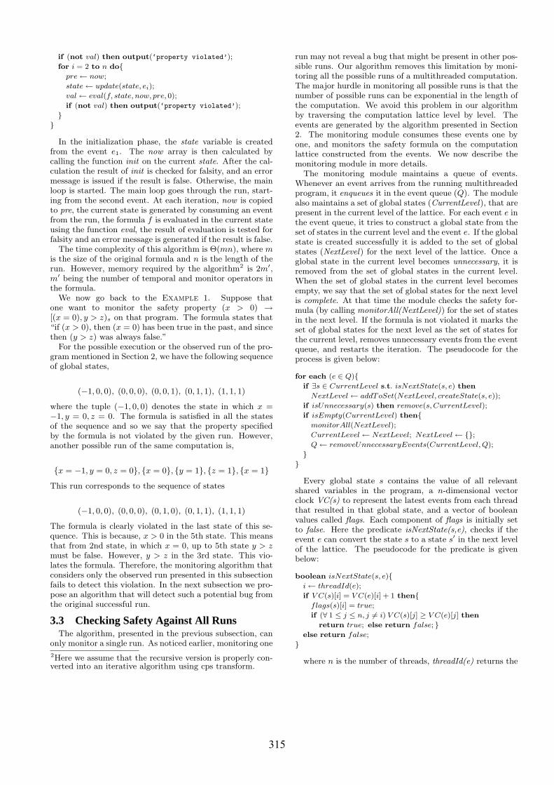
if (not val) then output(‘property violated’);

for i = 2 to n dopre ← now;

state ← update(state, ei);

val ← eval(f, state, now, pre, 0);

if (not val) then output(‘property violated’);

In the initialization phase, the state variable is createdfrom the event e1. The now array is then calculated bycalling the function init on the current state. After the cal-culation the result of init is checked for falsity, and an errormessage is issued if the result is false. Otherwise, the mainloop is started. The main loop goes through the run, start-ing from the second event. At each iteration, now is copiedto pre, the current state is generated by consuming an eventfrom the run, the formula f is evaluated in the current stateusing the function eval, the result of evaluation is tested forfalsity and an error message is generated if the result is false.

The time complexity of this algorithm is Θ(mn), where mis the size of the original formula and n is the length of therun. However, memory required by the algorithm2 is 2m′,m′ being the number of temporal and monitor operators inthe formula.

We now go back to the Example 1. Suppose thatone want to monitor the safety property (x > 0) →[(x = 0), y > z)s on that program. The formula states that“if (x > 0), then (x = 0) has been true in the past, and sincethen (y > z) was always false.”

For the possible execution or the observed run of the pro-gram mentioned in Section 2, we have the following sequenceof global states,

(−1, 0, 0), (0, 0, 0), (0, 0, 1), (0, 1, 1), (1, 1, 1)

where the tuple (−1, 0, 0) denotes the state in which x =−1, y = 0, z = 0. The formula is satisfied in all the statesof the sequence and so we say that the property specifiedby the formula is not violated by the given run. However,another possible run of the same computation is,

x = −1, y = 0, z = 0, x = 0, y = 1, z = 1, x = 1This run corresponds to the sequence of states

(−1, 0, 0), (0, 0, 0), (0, 1, 0), (0, 1, 1), (1, 1, 1)

The formula is clearly violated in the last state of this se-quence. This is because, x > 0 in the 5th state. This meansthat from 2nd state, in which x = 0, up to 5th state y > zmust be false. However, y > z in the 3rd state. This vio-lates the formula. Therefore, the monitoring algorithm thatconsiders only the observed run presented in this subsectionfails to detect this violation. In the next subsection we pro-pose an algorithm that will detect such a potential bug fromthe original successful run.

3.3 Checking Safety Against All RunsThe algorithm, presented in the previous subsection, can

only monitor a single run. As noticed earlier, monitoring one

2Here we assume that the recursive version is properly con-verted into an iterative algorithm using cps transform.

run may not reveal a bug that might be present in other pos-sible runs. Our algorithm removes this limitation by moni-toring all the possible runs of a multithreaded computation.The major hurdle in monitoring all possible runs is that thenumber of possible runs can be exponential in the length ofthe computation. We avoid this problem in our algorithmby traversing the computation lattice level by level. Theevents are generated by the algorithm presented in Section2. The monitoring module consumes these events one byone, and monitors the safety formula on the computationlattice constructed from the events. We now describe themonitoring module in more details.

The monitoring module maintains a queue of events.Whenever an event arrives from the running multithreadedprogram, it enqueues it in the event queue (Q). The modulealso maintains a set of global states (CurrentLevel), that arepresent in the current level of the lattice. For each event e inthe event queue, it tries to construct a global state from theset of states in the current level and the event e. If the globalstate is created successfully it is added to the set of globalstates (NextLevel) for the next level of the lattice. Once aglobal state in the current level becomes unnecessary, it isremoved from the set of global states in the current level.When the set of global states in the current level becomesempty, we say that the set of global states for the next levelis complete. At that time the module checks the safety for-mula (by calling monitorAll(NextLevel)) for the set of statesin the next level. If the formula is not violated it marks theset of global states for the next level as the set of states forthe current level, removes unnecessary events from the eventqueue, and restarts the iteration. The pseudocode for theprocess is given below:

for each (e ∈ Q)if ∃s ∈ CurrentLevel s.t. isNextState(s, e) then

NextLevel ← addToSet(NextLevel, createState(s, e));

if isUnnecessary(s) then remove(s, CurrentLevel);

if isEmpty(CurrentLevel) thenmonitorAll(NextLevel);

CurrentLevel ← NextLevel; NextLevel ← ;Q ← removeUnnecessaryEvents(CurrentLevel, Q);

Every global state s contains the value of all relevantshared variables in the program, a n-dimensional vectorclock VC(s) to represent the latest events from each threadthat resulted in that global state, and a vector of booleanvalues called flags. Each component of flags is initially setto false. Here the predicate isNextState(s,e), checks if theevent e can convert the state s to a state s′ in the next levelof the lattice. The pseudocode for the predicate is givenbelow:

boolean isNextState(s, e)i ← threadId(e);

if V C(s)[i] = V C(e)[i] + 1 thenflags(s)[i] = true;

if (∀ 1 ≤ j ≤ n, j 6= i) V C(s)[j] ≥ V C(e)[j] then

return true; else return false; else return false;

where n is the number of threads, threadId(e) returns the

315

index of the thread that generated the event e, VC(s) re-turns the vector clock of global state s, VC(e) returns thevector clock of event e, and flags(s) returns the vector flagsassociated with s. Note, here flags(s)[i] is set to true ifV C(s)[i] = V C(e)[i] + 1. This means that e is the onlyevent from thread i that can possibly take state s to a states′ in the next level. When all the components of the vectorflags(s) become true, we say that the state s is unnecessary.Thus the function isUnnecessary(s) checks if (∀ 1 ≤ i ≤ n)flags(s)[i] = true, where n is the number of threads.

The function createState(s,e) creates a new global state s′,where s′ is a possible global state that can result from s afterthe event e. For the purpose of monitoring we maintain,with every global state, a set of pre arrays called PreSet,and a set of now arrays called NowSet. In the functioncreateState we set the PreSet of s′ with the NowSet of s.The pseudocode for createState is as follows:

State createState(s, e)s′ ← new copy of s;

j ← threadId(e); V C(s′)[j] ← V C(s)[j] + 1;

for i = 1 to n flags(s′)[i] ← false; state(s′)[var(e) ← value(e)]; return s′;PreSet(s′) ← NowSet(s);

Here state(s’) returns the value of all relevant shared vari-ables in state s′, var(e) returns the name of the relevantvariable that is written at the time of event e, value(e) isthe value that is written to var(e), and state(s’)[var(e) ←value(e)] means that in state(s’), var(e) is updated withvalue(e).

The function addToSet(NextLevel,s) adds the global states to the set NextLevel. If s is already present in NextLevel,it updates the existing states’ PreSet with the union of theexisting states’ PreSet and the PreSet of s. Two globalstates are same if their vector clocks are equal. The functionremoveUnnecessaryEvents(CurrentLevel,Q) removes from Qthe events that cannot contribute to the construction of anystate at the next level. To do so, it creates a vector clockVmin whose each component is the minimum of the cor-responding component of the vector clocks of all the globalstates in the set CurrentLevel. It then removes all the eventsin Q whose vector clocks are less than or equal to Vmin. Thisfunction makes sure that we do not store the unnecessaryevents.

The function monitorAll performs the actual monitoringof the formula. In this function, for each state s in the setNextLevel, we invoke the function eval (as discussed in theprevious section) on s, for each pre array in the set Pre-Set. If eval returns false, we issue a ‘property violation’

warning. The now array that resulted from the invocationof eval is added to the set NowSet of s. The pseudocode forthe function monitorAll is given as follows:

monitorAll(NextLevel)for each s ∈ NextLevel

for each pre ∈ PreSet(s)now ← ; result ← eval(f, s, now, pre, 0);

if not result then output(‘property violated’);

NowSet(s) ← NowSet(s) ∪ now;

If the multithreaded program has synchronization blocks,

then we introduce, during instrumentation, a dummy sharedvariable that is read whenever we enter the synchronizationblock and is written when we exit the block. This makessure that all the events in one execution of the block arecausally dependent on the events in another execution of thesame block, so that the interleaving between them becomesimpossible.

Here the size of each pre array or now array is m′, wherem′ is the number of temporal operators in the formula.Therefore, the size of the set PreSet or the set NowSet can

be atmost 2m′ . This implies that the memory required for

each state in the lattice is O(2m′). If the maximum widthof the lattice is w, then the total memory required by the

program is O(w2m′). The time taken by the algorithm ateach iteration is O(w2m), where m is the size of the formula.However, if the threads in a program have very few depen-dency or synchronization points, then the number of validpermutations of the events can be very large, and there-fore the width of the lattice can become large. To handlethose situations we can add a parameter to the algorithmwhich specifies the maximum width of the lattice. Then, ifthe number of states in a level of the lattice becomes largerthan the maximum width, the algorithm can be modified toconsider only the most probable states in the level. We canspecify different heuristics to calculate the most probablestates in a given level of the lattice.

4. IMPLEMENTATIONWe have implemented our monitoring algorithm, in a tool

called Java Multi PathExplorer (JMPaX)[1], which has beendesigned to monitor multithreaded Java programs. Thecurrent implementation, see Figure 1, is written in Javaand it assumes that all the shared variables of the multi-threaded program are static variables of type int. The toolhas two main modules, the instrumentation module and themonitoring module. The instrumentation program, namedinstrument, takes a specification file, a port number, and alist of class files as command line arguments. An exampleof such command is

java instrument spec server 7777 A.class B.class

C.class

where the specification file spec contains a list of namedformulae. The specification for the example discussed inSection 2 looks as follows:

F = (A.x > 0) -> [(A.x = 0),(A.y > A.z))s

where A is the class containing the shared variables x, yand z as static fields. The program instrument instrumentsthe classes, provided in the argument, as follows:

i) It adds access and write vector clocks as static fields foreach shared variable;

ii) It adds code to create a vector clock whenever a threadis created;

iii) For each read and write access of the shared variables inthe class files, it adds codes to update the vector clocksaccording to the algorithm mentioned in Section 2;

iv) It adds codes to send messages to the server at theport number 7777 for all writes of relevant variables.

316

To do so, the instrument program extracts the relevantvariables from the specification file.

The instrumentation module uses BCEL [5] Java libraryto modify Java class files. We use the BCEL library toget a better handle for a Java classfile. It enables us toinsert vector clocks as static member fields in a class, thatis otherwise not possible with the tool JTrek [13]. We alsomake the update of vector clocks associated with a read orwrite, atomic through synchronization. For this we needto add Java bytecode both before and after the instructionsgetstatic and putstatic, that access the shared variables.This task is easier in BCEL as compared to JTrek.

A translator, which is part of monitoring module, readsthe specification and generates a single Java class file,named SpecificationImpl.class. The monitoring mod-ule starts a server to listen events from the instrumentedprogram, parses them, enqueues them in a queue, executestranslator to generate SpecificationImpl.class, dynam-ically loads the class SpecificationImpl.class, and startsmonitoring the formulae on the queue of events. It issues awarning whenever a formula is violated.

One of the test cases that we have implemented is thelanding example described in Section 1. JMPaX was able todetect violation of a safety property from a single executionof the program. The safety property that we verified was:

↑landing→ [approved, ↓radio)s.

From a single execution of the code in which the radiowent off after the landing, JMPaX constructed a possiblerun in which radio goes off between landing and approval,and hence it detected the safety violation. This exampleshows the power of our runtime verification technique.

5. CONCLUSION AND FUTURE WORKWe have investigated the problem of runtime analysis of

multithreaded systems from a fundamental perspective. Wehave developed scalable techniques for extracting relevantevents and their causal dependency from an executing mul-tithreaded program. We have proposed and implementedalgorithms to check safety properties against the compu-tation lattice of a multithreaded computation. We havealso briefly presented our prototype tool Java MultiPathEx-plorer, abbreviated JMPaX, which, at our knowledge, is thefirst tool that can predict violations of safety properties ex-pressed in temporal logics from correct executions of multi-threaded programs. We have also shown that, despite thefact that our safety properties can refer to any state in thepast and that there is a potentially exponential number ofmultithreaded runs to be analyzed, one does not need toactually store the previous states; one can analyze all themultithreaded runs in parallel, by traversing the computa-tion lattice top down, level-by-level.

Three major contributions have been made. First, wehave nontrivially extended the capabilities of systems likeJPaX and Java Mac, by providing the ability to predictsafety errors from successful executions; we regard safetyprediction as an important trade-off towards avoiding the in-herent complexity of full-blown theorem proving and modelchecking; we are not aware of any other efforts in this di-rection. Second, we have defined the notion of relevantcausality in multithreaded systems with shared variables

and synchronization points and we have provided a tech-nique of implementing relevant causality based on vectorclocks. Finally, we have implemented a modular prototyperuntime analysis system, JMPaX; modularity comes fromthe fact that its instrumentation module can be used to-gether with other computation lattice analysis tools, whileits safety computation analysis module can be used in anyevent based setting, for example a distributed system. Infact, we intend to soon extend our work to analyzing ar-bitrary distributed systems at runtime for not only safetybut also other properties of interest. There are also planson developing a predictive analysis runtime environment forboth multithreaded and distributed systems, as well as de-veloping a GUI for JMPaX that would make it easy to useand understand by ordinary software engineers. Since ourwork is partly sponsored by NASA, we also intend to soonuse JMPaX on real-world NASA-related large applications.

6. REFERENCES[1] Java Multi PathEXplorer, March 2003.

http://fsl.cs.uiuc.edu/jmpax/.

[2] H. W. Cain and M. H. Lipasti. Verifying sequentialconsistency using vector clocks. In Proceedings of the14th annual ACM symposium on Parallel algorithmsand Architectures, pages 153–154. ACM, 2002.

[3] C. M. Chase and V. K. Garg. Detection of globalpredicates: Techniques and their limitations.Distributed Computing, 11(4):191–201, 1998.

[4] R. Cooper and K. Marzullo. Consistent detection ofglobal predicates. ACM SIGPLAN Notices,26(12):167–174, 1991. Proceedings of the ACM/ONRWorkshop on Parallel and Distributed Debugging.

[5] M. Dahm. Byte code engineering with the bcel api.Technical Report B-17-98, Freie Universit at Berlin,Institut fur Informatik, April 2001.

[6] J. E. M. Clarke, O. Grumberg, and D. A. Peled.Model checking. MIT Press, 1999.

[7] C. J. Fidge. Partial orders for parallel debugging. InProceedings of the 1988 ACM SIGPLAN and SIGOPSworkshop on Parallel and Distributed debugging, pages183–194. ACM, 1988.

[8] K. Havelund and T. Pressburger. Model CheckingJava Programs using Java PathFinder. InternationalJournal on Software Tools for Technology Transfer,2(4):366–381, Apr. 2000.

[9] K. Havelund and G. Rosu. Monitoring Java Programswith Java PathExplorer. In Proceedings of RuntimeVerification (RV’01), volume 55 of Electronic Notes inTheoretical Computer Science. Elsevier Science, 2001.

[10] K. Havelund and G. Rosu. Monitoring Programs usingRewriting. In Proceedings, International Conferenceon Automated Software Engineering (ASE’01), pages135–143. IEEE, 2001.

[11] K. Havelund and G. Rosu. Runtime Verification 2001,volume 55 of Electronic Notes in TheoreticalComputer Science. Elsevier Science, 2001. Proceedingsof a Computer Aided Verification (CAV’01) satelliteworkshop.

[12] K. Havelund and G. Rosu. Synthesizing monitors forsafety properties. In Proceedings Tools and Algorithmsfor Construction and Analysis of Systems(TACAS’02), pages 342–356, 2002.

317

[13] JTrek Compaq Corp.www.digital.com/java/download/jtrek/.

[14] M. Kim, S. Kannan, I. Lee, and O. Sokolsky.Java-MaC: a Run-time Assurance Tool for Java. InProceedings of Runtime Verification (RV’01),volume 55 of Electronic Notes in TheoreticalComputer Science. Elsevier Science, 2001.

[15] I. Lee, S. Kannan, M. Kim, O. Sokolsky, andM. Viswanathan. Runtime assurance based on formalspecifications. In Proceedings of the InternationalConference on Parallel and Distributed ProcessingTechniques and Applications, 1999.

[16] Z. Manna and A. Pnueli. Temporal verification ofreactive systems: Safety. Springer-Verlag N.Y., Inc.,1995.

*

[17] F. Mattern. Virtual time and global states ofdistributed systems. In M. C. et. al., editor, Paralleland Distributed Algorithms: proceedings of theInternational Workshop on Parallel and DistributedAlgorithms, pages 215–226. Elsevier science, 1989.

[18] K. Sen, G. Rosu, and G. Agha. Runtime safetyanalysis of multithreaded programs. Technical ReportUIUCDCS-R-2003-2334, University of Illinois atUrnaba Champaign, April 2003.

[19] S. D. Stoller. Detecting global predicates indistributed systems with clocks. In Proceedings of the11th International Workshop on DistributedAlgorithms (WDAG’97), pages 185–199, 1997.

318

"!#$&%(')*+,*.-/0'1*2345 6879$:1!<;=> * *0?@,>

ACBEDF)BEGH9IJLKNMPO>Q RTSVUXW@YZH\[)G]6^L_N`ba>c*dfeg_Nhidj)kmlLnpoqkmefnpogc RVr _s^ktofefhu_N`>evnpwyxnzh/^|+ef_soa~_N`|_

`+~p_sodf~ecnpw1~`nz~d3kme ofl|k`|kmx|khu^kt~z`+f JLKNMPOXGH\[)G,LOzKUXMPUXODFXU

ps f¡L¢£E¢¤¥§¦¨© ª«g¬¥­¤§®q¯X°X±P¡+²+³´¨g¬µ¢¨¶¥§«g©·«µªf¸¹¥­£s°ºN¥­¬µ¢µ»¦©·¨g°P°«½¼¾¢¿g«g© À#¤¥§«g£Á¨¬¸°P¤«¦®¨°P¤¥§¦/«ºN¤§¥­¯X¥Ã¨g¤¥§«g£<¤Ä¢µ¦®q£s¥§ÅÀs¢°ÆÇ ®¢)¤§®q¬µ¢P¢y¶È¨g°P¥§¦y«º¢¬È¨g¤§¥§«g£s°)¥­£É¡²Ê¨g¬µ¢X°¢©Ã¢µ¦¤¥§«g£Ë|¯XÀ#¹¤¨¤¥§«g£É¨£Á»¦¬µ«°P°«g¿g¢¬ÆÌE¼´¤§®¢°¢y¤Í®q¬µ¢P¢Ë\Î+¢$¨¬ªgÀs¢¤§®#¨g¤«g£©Ï¸Ð¤§®¢$¦¬È«g°P°«g¿g¢¬1¥­°y¨vÀ#£s¥§ÅÀN¢©Ï¸2¡²Ñ«Pº¢¬È¨g¤¥§«g£ÁÆuÒv¢«½Ó\¢¬´¨g© ¤Ä¢¬£N¨g¤¥­¿g¢X¥Í£¤Ä¢¬ºN¬µ¢¤¨¤¥§«g£s°X«½¼)¤§®¢y¶µ¨°P¥§¦@¡+²Ê«ºN¹¢¬È¨g¤§¥§«g£s°µË¨g£Á»y¤§®¢£)¼«¦À#°«g£Ð®«g®¢0°º¢P¢µ»«½¼¦P«g£¿f¢¬¹ª#¢£Á¦¢L¦®¨g£qª#¢°Î>¥­¤§®X¤§®¢\¦®#¨g£#ªq¢L¥­£¦¬È«g°µ°«g¿f¢¬m¼P¬P¢ÈÅÀs¢£N¦¸¥­£V¦P¨g°¢C«Ä¼°«¯y¢2°P¥­¯\ºN©Ô¢vº¨g¤§¤Ä¢¬£©Ã¢È¨g¬£s¥­£#ªºN¬È«q¶©Ô¢¯X°ÆÌÀ#¬´º«g°P¥­¤¥§«g£/¥­°@¤§®#¨g¤1«g£s© ¸2¤§®«g°¢¦P«¯y¶¥­£Á¨g¤«g¬¥§¨g©,«ºN¤¥­¹¯X¥Ô¨g¤§¥«£Õ¨g£N»°¢È¨g¬È¦®ºN¬È«q¶©Ô¢¯X°yÎz®¢¬P¢¦¬µ«°P°«g¿g¢¬°1°P¥·ªg¹£s¥ Ö¦P¨g£s¤§©Ï¸v¨½Ó\¢µ¦¤*º¢¬Í¼«g¬¯1¨g£Á¦P¢1Ψg¬¬È¨g£s¤,¨g£C¨ºfºN©Ï¥§¦P¨¤¥§«g£«½¼¡²i¥­£s°µ¤Ä¢µ¨»«½¼°P¥­¯\ºN©Ã¢¬|¬È¨g£Á»«¯×°¢µ¨g¬È¦®1¨PººN¬È«¨¦®¢°ÆØ@ÙÚtÛ)Ü gÝfÞ ª#¢£E¢¤§¥§¦¨g© ªq«g¬¥­¤§®¯X°µË´°P¤«¦®¨g°P¤§¥§¦6«ºN¤¥­¹¯X¥Ô¨g¤§¥«£Ëtº¨g¤§¤Ä¢¬£3©Ô¢µ¨g¬£s¥­£qª

ß à9áâã)ä(å*æ@çá|èé2ê2ë\ç|âè@æ.çèíìïîðñòpñóôÄõÕö#÷ øsùqúôóûüýuþðLÿ "!#$

%&'()%+*,%&-.%&//)012 3!+4 %+!)*,5%+/)(6% .07987#%&+48/)0: %&/;(6 %&<) . >=?&<@%+/'/)0'/#<@ "6.+.>%&/:A1ðLÿB!#.=C<)/)0D/ <)*,> <)E2(#(#+%&.%&/)%+/F/9<#*7G> H() 7#&*I0)$*;%&/)KJL!) MÊúöqòONùqüôPfñ"NV÷Ãùfõö#÷ýñöqúõûQ,!#1(6 "*,>> (R.%&S()(#&%&.7#&AUT9*,V>W)*5(6+.XY<)3!Z()(#&%&.%+/)[ = %+<)(6 /K0)%+/\/#0K .4/)%+%&/K() 7#&*, ]2^/#0 "%&/)%&/)4_!)J%&4!?X` %+a#%G/#<@ ":/)bJ c 5 deA

ðLÿF7O.+/)4,f,.&Sñ3g#ù#÷ihÁóôÄùqòpöqú3j2ö#÷ øùqúôóûü@ýkl!)V$&<@%&/Zm,(6 %&<) L(# 76+.*n%+[<)4!?S=@%,=+=@%+/)4',(O()$<#&%&/S4/?EoC >(# /90,p>_L %&/)4_L4/).3qr *s/)L4/#> "%+/,!)L/)W .9<)/?%&t@ l*_S/9<#*7G> 4./)> "%&/#?!)X0)%+ 0fu9<#+%+b856!)U(G(6<)&%&/,%&m ."!#0GAv !#[4 0)/).G%&/)0)%+=@%+0#<#R 4?/)%&*_#^J&O^./?%+ S(O()$<#&%&/#%+mu9<#/?%+a#0w7 8w/_()() () %2mx|óòpñýýOy"hNòpõóôùqò= !#4/) %&/)4A

v !#^!@ 76%+X(G> "%+/)m%+/¾ðLÿz%&/_. 0#/)JL%!5!) %&4%+/#G76%+&4%&.:%+/)(6% "%&/:6 z+&0Éýñ÷ÃñõóôÄùqò#|ü_hÁó½ö#óôÄùqò/)0uõúùqýýùgqñú3A

|zñ÷ÃñõóôÄùqò<@ U!#.@*,/)45!)[<@ ./?U(O R:4./)!#4/)~(R2 /)JL!)Hxóòpñýý'%+E*_(6 "2768D!)%&4! *, S&%+c.8,7GXc?()%+/f!)S/)>W ^4./)> "%&/'4./)L(O #!#/!#[4./)S(6> /#^:&J> a)/#Amb/'!)S./?>W U: "!#$%&S()%&*,%+-%+/G9!#f*,.=?.w "!)%&.l!#!#.=?L(# 90#<).0*, 0).% "7#&<@*,_%+/1!)'(6, *_ &%c?.8\p7O3!)/K%&/p!)5C<@<@ 5!#/p!)5*,=? "!#%&.[!#!#.=&0H,&LC.=? "276+<@.*,.A

hEó½ö#óôùqò%& "/)0)*H b8 (#%&.&8;*;+R(O> <@ 7R2%&/;!#%+/? 0)<#,*, "/)0#*,%&-.%&/Q%&/?~!)H. "!GAM_/7G= %&>J.0M;~=?> %&/M'#%(#(#%+/#4\p76%ot .l%&/M!)%+,4./)2qm%+/'4/#S.u9<)./).^:*_ "/#0)*_+8;.+.>.0GY 4/@$%+*,() ./?%+/~!)5.<@ /94/) "2%&/GAF!)%+&_r/~0) %$*_./?"6%&/'.[G%&/)0)%+=@%+0#<#R&%+= %&/)4w 4?/#%+*,)*w<@"%+/).//)<@ *;%+/?"%&/)%&/)4[ `=?/w .%&/)4S*,øsñòñóôÄõ[Nqôrg#ñúýôótj^%+/(O(#<)2%&/)?YJ^0)%&<#Y%&/;> AYb/V(6 %&<) .%&/V!)^./?>W O93!#%+S(#%+*,%&-.%+/G9*w<@"%&/)l!)+(;%&/;>W (#& %+/)4*, !); "!(6f!#/JL!#VJ<)&0\7O;b89(6%+&+8>W (#& .0JL%!H.+.>%&/E/)0E> = L/)+8R.A

+úùqýýùg#ñú%&^/;(O "2%&/;"!# "> %+%&LO!)yýñ"hmö#÷múñ úùNhmõóôÄùqò)kbJ0)%+O> ./?;4/)Hu9<)/).; H&0G/)0!)/D2(#() () %&.83!)/D<@7#u?<#/).'W@"!#/)40:A v ! <)!)bJf"!)%&&0@ /)[.u9<)./).%&/)!) %Y*,^ !).% Y4./)r *."!l!),bJH(6 /?`!)J>=?> .!);"!)%&&0@ /G`<)*,%+/)4/)/? %=@%R<@7#u?<#/).U!#.=?S7O./f 0=?> .) z&50)%&$r /? *."!_#!#%+ `(6 /9`J&#mr */#U/)!) .Al!6l7O./f 4<#0;!#.9%+/f.SR!)L/62<) "6=?&<@%&/f/)0*,/?8593!#%+U()%&*,%+-2%&/5() 7#&*,+%+c?!)U%&/?> ">%&/O!#L!@ L76%&S(O "2%&/)/)0;!)S8@/) 48f*,/)4V!).*%+^JL!#*;c?@ðLÿ(OJ r<)O%&/fa#/)0)%&/)45!)%&4!fa)/).+<)%+/)/#0!#L> =?> X(#.8H_./? "G +%+/H!)%&X8@/)> 48?A

b/V!#%+(R2(G> .J^*;%+/#8VC <)Y/w!)l +@!#^> = (G> "%+/Gk5!)Js!#;/?=?> 4/#fXðÿs%&wO.>.0\!#õúùqýýùg#ñúúö#ó½ñX%&L= %&0GO/)0GR%&/E(6 %&<) .RS%+[()() ?"!).-> )A_; 4<)_!#V> = V%&!),/)+8K*,/)4H!)_7R%&ðÿM(O> "%&/#`!#%&m <)+8_z(O.%+a#UC.<@ XO4./)>%&X&4$ %!)*,) "!) U!#/Z_C*,%&+% L(O "2%&/r *!) X "/#0)*. "!~/)0p*;"!)%&/)w&. /)%&/)4;."!)/#%&u9<).R/)+8Q%+/~0)%+4<)%&)Av !#l/)/@$e/).4&%&4%+7#&Sr .u9<)./)>8_O .=? ^%+u?<#%L./?%&r <)..r<)()%&*_%&-.%&/~= %ðÿ%+/*_,.:JL!#%+&,r &() ">%&.(6<@ (Oz .=? 54>!#> z<)/)/#. 8%+/F!)> .z%+E%+&+<# "2.0DJL%!*,%+*_(#&K(6> /F+ /)%+/#4>W)*5(6+.AT9*_'&/)50@ ".JL/1r *<@ 5W (O> %&*,/?Hot0)%+$<).0~%&/13]?qL 5!#,ot%CqX!)53!)%+.5m!#_><6`> = u?<#/)8X%&/D.~!#p() 7#&*,'JL!) p> =?> E <)C<)U%+'+%+c?+87OZ[<)*_'%+*_(O "/).Zr f!)E(O.0^./?=?> 4/).,l!#_%&/)%+%&m(O(#<)%+/K!#_/),^*;W9$%+*;Ya)/#/#0~!#;ot%+%CqL!)_4 0~ .=? V/)0K*w<@"%+/ u?<#/).%+.,ot V u?<#/)8Z "/#4.3q[./K7O_0)(O/)0#/?V//)/#!#> .A v !#w*;%+/~&/p!#[J5*_(#!#%&-5!) %&/p%+[!#ot%+%&%rqS%+l!)¾ðLÿ/?=? 4./)_ "2. _%&/)0)(O/)0#/? /) 8%+/)0#>(O./)0)/9Y@!)^> =?> ` "!#/V!)(# 76+.*2`!#/)0%+U/)X549 0ðÿ2(#(#+%&.%&/G)%+/'(R2 %&<#& .@Jz0)0)<#zr *!)>W)*_(#&%&/,3]!62Uot%=6qO%&)U(R2 %&<#& ´ðLÿ\0) u9<)%+J&%+/Hw4%+=?//?>W JL!)/'!)S() 767#%&+%+b8' =?> U%&c()

"G3e3 3¡e¢23£¤¥ e£¦i e§ ¨3©e¢¦iªG2««¬S23:3§ ­G¨ªG®«Ye¢2«`3ªe«¯6®2¡.>°ie«S«23¡2±>¢S¦ G¦iª².e¢2«m³"e«e¦i3§®«2« ´eª3° £>¬2>µµl¡e"e¦i>2ªG¬2« ³« 2¬[3Se¢«`>£« e«`³2£3®2§i«µ3¢2>¬z>¬[¦ eª£« ³2£«ªe« e"e¦i>?©e¢2«m³3³2¡2§i3e¦i3Sªe¦i¶ «3©2>2¬Se¢«[·e±>« 2« e¦i`¬2¦ ¸>« £ªe¦ C¨.¹>° e¢2«m¦i¦ e¦i>§)º&¡2ªe¡23§i§ ¨L£>2¬>µU§ ¨L¢2>ª«»R³3³2¡2§i"e¦i>?¼

319

=? 8'*;&G X=./>X5-.> )@!)/H¾ðÿ$76.0E()() ?"!H%&&%+c.8,/K=?> c@%&+&C m!#m(6 %+.<)& () 7#&*/)0 ^()(#&%$%+/0)*;%+/:Az<)_H(6.,/) "%&/?%&/K!),0)%+.<)%&/S<@ ,W9(G> %&*_./?_%&/D3]ZJ*,81C <),/ ot%+%&%Cq$"ot%=6qw/#0/)+8'7# %+)8' >#.>L/!)!#> X(O%&/?S7O=?A å*æ@çã)á2á|ã0ç|âgæíìïî Éã)á1ç|âèæ

s/)>W 7# %+)8 0)%&<) !)!) 76%& ðÿ (G> "$%&/)A`\X%&/?> () l/)0,3!# "> %&-X.+.>%&/:?*w<@"%+/f/#0 .=? 5%&/\> *,w!);76%&f/).>()wr * ÷­ñöqúòmôòNø'/#0ù óôü@ô&Pfö#óôÄùqò)AS<) ,*;%&/(O%&/?,%&_!#.JL!#%+&.+.>%&/Q/#0*w<@"%&/G^%&/<@ ,=@%+Jl./7O' 0)%++81<)/)0#> 0JL%!)<@/?8K .r /).,H7#%&+48`/#<@ "l>=?+<)%+/\ w4./)>%&f+4$ %+!)*, ñúýñ>L!)~> =?> H(O "2%&/B%&'(O.<)&%& +8 ðLÿ(O "%+/GA v !) C 6%&/)5/?8H() 7#&* !#S/E7OV=?.07 8ðLÿ /p&;7OV+=.0Z798E!)> [ "/#0)*_%&-.0Z& .. 3!."!)/#%&u9<)./#8!)l() 7#&*,JL!)> L/)/@$e/).4+%&4%7#&^() 7)$7#%&&%b8U> =?> w*;2c?.wE/)%&0)> "7#&;(O r *;/);0#%+r$C> ./)G <)+8p0) =_'7O5./)%+0#> 0 ðLÿ()(6+%&.%&/#A %&4 <#`*;!)*;%+@r *w<)2%&/5)!)^!) ^76%+()$ "%+/)L./H7OC<)/)0G6A 4@A&#%+/+ûÁö ó½ñúzVU ]2A

wa)Wp*,,/)"%+/K/)0~ *,%+/)&48~<).0~!@ <)4!)<@!#(6(O .A# `/) >/#;4./)S%&YX8@*V7O9 * %+!)> !#L> /62 8f+(#!#7O> !#"?9 %+l7#%&/# 8;<@7#"?Av !#' 4?/)%&*_5 U4/?U S4%+/#4VV7OL () ./?0^a)$/#%L %&/)4lR4./)l=?> l!)S+(#!#7O.A v !)L=&<#%+/,C<)/)$%&/Z%+/(ðLÿ %+S&&0;xóòpñýý"O%+/Z<@ [6%+S*;(#S*,a6/)%O7#%&/# 8; ^> /# 8; %+/#4%&/?57G<#/)0)0'G%&/?.4 =+<).AS= "4Va)/#[f4./)> "%&/Z 4?/)%&*,[%&[%+*_$(68Z!)_ %!)*,%+5*_/~&`%+/)0#%=@%&0)<#` 4?/)%&*,%$Oa)/).=+<).A\~!#&[<)~7#%&&48S*,!).*;2%&H/)0D*_(#<@ .%+./)X> *,%&/)+4%&l%+/9> "!6/#47#8_!@ <)4!)<@!#U(6(O> .C Y%&/)"/).!)l *_0ùqúÄøsöqòmô§ýü_tögøñòtótÁôòONqôrgfôNhtö#÷./#03ýóúô§òNøþµùy)øñòpñý$ùqúyý"j#ü &ù#÷Ïý[ <#0E8@/)/?8@*,<)+8H!)> JL%!GA' )( *D*WµD*O MµJ,+|zñ÷ÃñõóôÄùqò%&,!)ZðLÿJU.8z"!)%&>=@%&/)4úñô§òyùqúõñü3ñòmóX Éñ ÷­ùqôó½ö#óôÄùqò_:!)z0)%+ "7#&[(# (G> %&^!#U!6=? 0)8;7O./0#%+..=? 0GAUb/Z<@ [%+*_(#&w*_ 0).m&%+/GR4%+=?/p,+&$%&/V@ %&/)4`/#0!)%+ Y%&/)0)%+= %&0)<#?a#/)=&<)/#l Y*, &J a#/)[ %&/)4z 5"!)/p;7Gw0)%&. 0).0G:/#0Z >(#.07 8E(#%&[`!)V*,w/9<)*V7O> zm!)%+4!Za#/)[ %+/)4A v !9<#!#L%+-.SO!)X(O(#<)2%&/, .*;%&/)l!)L*,97#<@^%+V4./)>%&u9<#&%%&K '%+*_() =?01= %Z.+.>%&/:A v !)./14/)%+'(G> "$%&/),[*w<@"%&//)0Q> = f H(O> C *,0M/!#> >7 8%&*_() =?0H(G(6<)&%&/GA- 4/) "++8z.+.>%&/%+Z*,3!#/)%&* !62E/#<@

!62!)5*, 5a)%&/)0)%+=@%+0#<#+ w'() (64?25!).% øñòpñóôÄõü3ö#ó½ñúôö#÷Y!)Er<)<@ E4/#> "%+/),JL%+!Q!)%&4!)> f() 767#%&+%+b8!6/H!)+.Ua#L%+/)0#%=@%&0)<#+A,.[/##&%+/H/7Gz=@%+J0úñôò.yùqúõñüvñòtó,ü3ñõûÁöqòmô§ýü_kL49 0p4/)w(6 /)O%&/p4./@$ "t6./)0H;7O %&/)r .0Er * /)w4./)> "%&/E,!)/#>W .JL!#> .Y&J1a)/).Y4/)l(R2 /)Y!#.=UX7G&.JX$.=?> "4^() 7)$7#%&&%b8_R<@ =@%+=@%&/_3!_4/) "%+/,/)0G9/)u?<#/?+8?/)0,0)%&()(O2 z+4>!) X%&/!#&/#4_ <)/ 0/2A

' ' 1 U G MÈJ2+v !#> X U`&.`bJz0)%+O /?m &`6*w<@"%+/)9/)0_!)/#bJ\0)%G> /9_JU.8@,S%&/?> () %+/#4~!).*HAS/)E%+,!)*;&(G> <@ 76%&/=@%+Jk5%+/ 0) VE() >=?./?V!)'+4 %!#* *4%+/)4Q<)"c oC798?.8() *;<@ .8K/?=? 4%&/)4EEH& .

(#%+*w<)*'q"~ "/)0)* *w<@"%+/7) 2c@,!)H<) /?;.u9<)%&&%7)$ %+<)* <)/9%+=./?<#&8? <)+8~4&7R&+8~"7#&,./@a#4<@ "%+/%+` 3!)0:A3[/)!)> m &UR*w<@"%&/#m%&`!62m!#>8w./#7#+U!#>W (#& "%&/;O!#L(6 ^O!#L./@a#4<@ "%+/f(6L!#. %+/.;760&<)cJL%!\!)f%+/)%+%^/@a#4<@ "%&/G`J<#+0!#.=?/)>=?> l7O./; ."!#0f&+8_=@%!)S&%+/f/)0f =?> ()$> "%+/)A4 %&*5(6+>W)*_(#&z%+X/()%&*_%&-.%&/'() 7#+.* =?> > /# 85+(#!#7O>5 !#"XJL!)> U!)U %&/)4/).90#%+/)4O/984&76++8,()%&*;R+<)%+/f%&/)&<)0).l!#L8@*V7O6!598?l!)S%&/)%$%&U(O(#<)%+/Q[ %&/)4;%&/).+<)0#;8@*V7O+7 /)0 /)8?A8^+2 +8@JL%+!)<@S5/)/)- _() 767#%+&%+b8'*w<@"%&/E.%!#> %&/?9!_)/#,.u9<)./)Y&%+/Z/)0E =?> S(O> $2%&/)@ö#÷­ùqòñLJ<)&0p=?> S7O57#+w; .3!p;4&76++8Z(#%+*;/@a#4<@ "%&/:A

v !9<)^JL!#%+&E&>%&/() =@%+0). ñ ÷Ãùqôó½ö#óôÄùqò\S!)H4 0 "%+U%&/H!)z() ./?S4./)> "%&/G)*w<@"%&/)U(# .=@%&0)ÐúöqòONùqü,ô&Pfö#óôÄùqò)!) >798M>W (6/)0#%+/)4\!)E "!B/)0Q/6276+%&/)4Vñ" ÷Ãùúö#óôùqòKX!)'./@a#4<@ "%+/)5!#_!)> JL%&'*;.8\7O'%&/#>$%+7#&A'b/7#%+&4%&.m *,JL!)%+&,!);&>%&/\(G> "%+/G: <),5%&/.'yòö#óthÁúö#÷Lýñ÷­ñõóôÄùqò)lt=? 5!)'<@ =@%=m >$() 0)<)>%&/'/)0'<)+%+*;S/9<#*_ %+R0)*,%+/#/).[O!)Sa).!)*w<@"%&/E(G> "%+/E/6276+.X .%+/E/)0E&/)4$> *(O> $%+./) ù hE÷Ãö#óôùqò\NqôCgqñúýôótjA

' <; =ÉBEJLKNKsJ?>\D>BA@CBD+XM)EU)D*WGF SVYD!)%&&E&%+/%&f*, 0)L[ %&/)C .*,/9'/)0*w<@"%+/;C * m "/)0)*n(G> <@ 76%&/GG>W (#%&/)%&/)4¾õúùqýýùgqñúL%&/Z!#> *,,C*,%+&%2 ,\/M/)4%&/) , fK*_(#<@"%+/#X.%+./?%+JL%!5/)zc /#.JL&0#4U)76%+&48w%&`*w<)3!_*, 3!#+&/#4%&/)4)A3HU%&$+4%+++8 .=? XS(O.<)&%& C.<@ *ýñ"hmö#÷Áúñ úù2Nhmõóôùqò#A`D!#%+&[%&/)4&S> =?> (O "2%&/;7ObJ/;bJV %&/)4^8@*7G&V./K%&/K() %+/#%+(#+fJU.8@7O_%&*w<)&.0K=@%H/()$() () %&Xu?<#/).XR%&/)4+$e8@*7G6*w<@"%&/)?!#%+0#9./)+0_V/#<@ ")%&/? () >"%&/;R> =?> l%&/_ *,R*w<@$"2%&/)A Iz*,+8*w<@"%&/#V ,<)()(O0\7G,%&/) u9<)/?. "/#0)*Y/#0K%&/)0)(O/)0#/?V^/);/#!#> .: "!) z!6/K=?> 8*,*_/KJ /#0Gz%+/D!)KK9$ *w<@"%&/#%$X%&*V<#&%&/)4!#*,;%&/)4+f> =?> .Y!)%&4!)+8K*w<@<#&8. .&.0\/)0\/)/@$ "/#0)*LAl!#m7O./;2 4<).0_!#!)X(OJ> l,ðLÿM*,() %&*;2 %&+8 * !)(OJ> ,S> =?> ~ ]2eA\ >(6!@ "!)%&57 82 $4<#%+/)4f%&/>]5!#L!# ðÿ 2(#(#+%&.%&/)L!#S<#V&%++V S/#> = L/#002 '(O> C * %&/)0)>(G/)0)./?+8M[!)Z> = () 767#%+&%+%+.[ p/#H4/9<)%&/)<ðÿzU%+/B!#'!#p<#/)0)> +8@%+/#4() 7#+.*,z/~7Ow 0)%++8~/)0 : <)NM;%&/?+8p=?.0~JL%!@$<)L4./)>%&+4 %!#*_[+4>!) .A

O PQ´ççã)áæSR/ãáæ2âgæTVUDWXYZ\[ã\V/)J 0).> %+7OV<@ z>W (O> %&*,/?R<@&%&/)!)V*;%&/ZC.$

<@ X!#[bJ_(6> /H+2 /#%+/)4_() 7#+.*,UJ!#.=?<)0#%+.0G() ./?L*_!)>W (O %+*,/9"G <#6/)0H!)/HC <)X/!)%+ L%+/9> () "2%&/E/)0E%+*_(#&%&.%+/)A

b/;7O!;(# 76+.*_ !)_ot%+/#%%rqm %&/)4ot ^]Èõûúùqü3ùqýùqüvñ`_q+./)4!p%&z.%+4!?.AVb/p!)wa) >l<) %+*_(#&5(6 /p&. /@$%+/)4>W (O %+*,/9!)Z4?S%+;>=?=?p(O(#<)2%&/ $4/)%&*,S [4/?S,!)V/#JL!)> V.3!p4./?.# () ./?0z;7#%&/# 8Z %+/#4'=?> [!)_+(#!#7Oa"?O./?"%+/)z%&/p% >() ./?"%&/."!1X!)'!@ f(6 /)kbV,f/#0cfAd[%=?./D %+/)4)_%~a)/#K%&K%&/)> 0 798 r K!)() ./)Mf3!;!).!@ M<@7# %&/)4A v !)JU 0%&4%+=?/% .(O%=?M,!#1/ <)*V7O> \, (O>%+%+/)

eaf [³2£3 e¦i«3©.e¢2«m£3ªeªe¸>«£G£3e«ª:3£«m¡2ª¡2>§i§ ¨L®>¨S3§i«3ª:>«m>£¬2«£G>°@µU3±>2¦ e¡¬2«m¢¦i±>¢2«£Oe¢2>Se¢2«mµl¡e3e¦i3[£"e«ª¼g f 2¬2« «¬?©3¦i^ >ªe«R>°2®2¦i2>£t¨3§i³2¢23®«beª©3ª¡2¢^µl¡e3e¦i32ª)3£«O¡22¦ih¡2«§ ¨¬« e«£µU¦i2« ¬l>2 «Oe¢2«RC­O`ªte£¦i2±>ª eY®«O£>ªªe«¬¸>«£ ©>32¬ j kmlnpoqrtsuk`qwv6xzyq|w|zq~%nyj ©¢2¸>«®««[¢2>ª«?¼

320

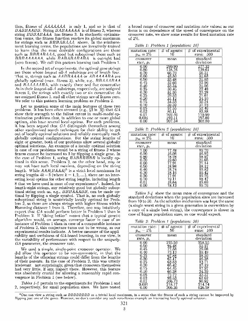
! <)za)/).E# %&E/)8/)0M%&H!#E##;A^T? %+/#4 # %&m#a)/)l JL!) . %&/)4# !#[a)/).] Azb/p "!#%&5(#%+*,%&-.$%&/E> *,6!)a#/)SC<)/)>%&/E ."!#S%[4+76*;W@%+*w<)*C V %&/)4V<)"!1## 27G.=?Afb/K!)_ .%+/#r $*,./?L&. /)%&/)4,> *,@!#z(O(#<)%+/)S %+> "%+=.8' "%&/).0B+ /!#Z!)*,p0).% "7#&/@a64<) "2%&/)~ !#<#"!1##V4 07#<@w<@7O()%&*,!);<)3!##VSJL!)%&+ ## %&H<@ %&4!?E760ot-.> 5a)/).3q"Am\z.&O!)%&(6> /&. /)%&/)4_"c 7#&* A

b/V!)^./)05>`)W9(G> %&*_./?!)^()%&*; 4/#^ %+/)4 _!)_JL!)2÷ÃùqòNøñýó´ö#÷§÷ ÿ ý"hp&ýóúôòNøqýz ,l&/)4!r<@ .Av !62[%&R %&/)4S<#"!~ # # 4&76++8(#%+*;ot*;WOA`a)/#[]q"@JL!#%+&#A 4)A+K#/)0 #V:JL%!W)8~!@ ;/)0Ka)=?;./#<)%=?S%+/!#%+ L÷­ùqòsøsñýóPö#÷§÷ ÿ<ý"hp&ýóúô§òNø#ý (O.>%+=?+8 l%&4/#0a#/)96!#V %+/#4SJL%!ZW)8bJf [%WE/).<@%+=?S U%&4/)05a)/).U/)0,+@!)> ` %&/)4m )a)/).`-.> )Az C> X_!)%&X(6> /H&. /)%&/)4_(# 76+.* 7#&* 9A

>w<#w*,/?%&/*,'U!);*;%&/1r<@ w!).;bJ(# 76+.*_Al!#7O./;./, .0potA 4)A+#>]z%+/~ ]2CqY!#$ðLÿ!#.J!)%+ [ ./)4!Zf!)wr<)&&z>W ./?[%&/uü5hE÷·óôC½üvù2Nö#÷)()$%&*,%+-%+/H(# 76+.*_S!#.#%&/p0#0)%%&/H;/)V S*, V4+76()%&*;@&!#.=?_>=?> "`& .Y()%&*; A# <)3!~() 7#+.*,%+_!#w7O./ 4<)01!#ÉðLÿ 0)%&%&/)4<)%+!1!).*,+=._*,/)4!) V "/)0)*,%+-.01. "!\."!)/#%&u9<).Vr w!).% 57#%&&%b8KZ4><@lR&9++85()%&*;#&<@%+/)^/#0_ &%2768_>=?/?<6&+8w .3!4&76++8()%&*,[/@a#4<@ "%&/#A # !)p %&/)4&/#4!#'.%+4!?L U4 2 . 7O!<@ U() 7#&*,L&&.J >=?> "G4&76++8()%&*;:&<@%&/#A2[/E>W)*_(#+V`_& .&8H(#%+*;&<@%&/%&/E.<@ L() 7#&*,XJ<#+0E7O_ %&/)4,a)/)zVJL!#a#/)U./)/#U7O[%&/) .0',]798;6%()(6%+/)4,5%+/)4&z4/)Amb/!#.' 7#&*I %&/)4 ## %&5& .++8()$%&*;m%&/K!)%&./)A 7#+.*9/K!),!#> !6/#0G*;.8~ *;.8\/)5!#.=?'<)"!1& .l*;W@%+*;@m0)>(G/)0)%&/)4p/!)f %&/)4&/#4!:AF!)%&+5o<qw%&[; %+S+ *;W@%+*w<)* C %&/)4w&/)4!)^dZ]foCJL!)> "` q"?!) [2 S/)w%+/? $.%+/#4V+ 6()%&*;C ^!) ^ %&/)4V&/)4!) %&/).+<)0#%+/)4w+./)4! !#mJU!#.=?U<).0,%+/_*,6<@ >W (O %+*,/9AYb/)0#0:?C &/#4!)$e%&4!9U %&/)4)/?8f %=?.8f4 0f7#<@U4&76++8f<@7O()$%&*; %&/)4Z<)"!1YA 4)A&3#fY./7O,*;0)f()$%&*;798H#%+()(#%&/)4';%+/#4&w8@*V7OA v !#[%+O/)f<#"!p4&76++8<)7O()%+*;S %+/#4%+f/)/? %+= %++8M& .&8Q(#%+*;LC 7)$&* 6X!)> V V+JU.8@L %+/#4LJL%!H!#%+4!) La)/).UJL%+!)%&/.z*,*,%+/#4w0)%&"/)5Sr * %.A v !) C /#[*,.8;%&/?<)%+%=?+8W (OX!#3ðLÿFJ<)&0H(O r *7O> L%&/ 7#&* !#/E%&/ 7#&* AHb50)%&/)4E7O> E*,/#!625Hb8 (#%&.l4./)>%&&4 %+!)*J<)&0Gm/=? "4m/?=? 4't> 5%+/.'L/%&/)"/).[ 7#&* S!#/'%+/'.[w*_(6 "276+[%&/)"/) 7#&* #!)%&L./ : .><@ <@ /)S<@L,7OJX /)4)RS<@ W (O> %&*,/?"9 .<)+`%&/)0)%&.A3Q7O> `*,.<@ U)!)U()(#&%$7#%+&%+b8'/)0<).r<#+/).U)ðLÿ$760H&. /)%&/)4))%+/<@ U=@%+J@%&!#= %&7#%&+%+b8E`(O> C *;/#JL%+!E .(OS,!)fhNòmô>hmñ÷ijðLÿF(6 "*,> .@!)> =?> L "2A

<)0Qp%&*5(6+l%&/)4&>$(O%&/?;> = ,(O> " .A\\0#%+0 &&.J !)%&(O " 7O~/#/)$e8 *,*,> %&z%&/D!#!)&/#4!#X!)O() %&/)4, %&/)4L<)&0E0)%+O> Lr *!)+./)4!)m!#%+ [(6 ./?Ab/p!)5.5 7#&* O!)%&[JU[<)> +8%+ &>=/?Y$G/)`<@ () %&%&/)48?4%+=?/V!62m> = Y!).*,+=.!60\=?> 8K+%+&%+X/98%&*_(6>V!)> A9.[J>=?> .!)%+VC.<@ JUw7#&<@+8K <)%mC w&+JL%&/)4ZH ./#7#+8~ "(#%&0./@$=? 4./)%+/ 7#&* ;ot.z7O.+Jzq"A

ö &÷ÃñýwK(O> "%&/L!)l>W (O %+*,./?r 7#&*,^/#0 m (O.>%+=.8?`C _*;&l(O(#<)%+/1%&-.AZ\'!#.=?;.0

57) ?0H "/)4Y> =?> z/)0E*w<@"%&/H "z=&<).6L<@ r <#V%+w/\0#>(O./)0)/#f!)f(O.0U/?=?> 4/#f/\!#> = U "@Jz!)J*,z <)+UC Ua)W@0*w<@"%+/ "mfA

ö &÷Ãñ,úù &÷Ãñüþ ù hÁ÷Ãö#óôÄùqò "*w<@"%+/H "k ! `4/?k ! Y>W (O %+*,./?"

"$# F &% <)/)kD/'%'% =?> *_/ "/)0# 0 " "( 0)>=@%%+/% A*)'% )'%@A+)'% ,,9Ai]% A % A*,'- ) A+-@% A.,/% -'- A.,/% /-9A /@% A*-'% d?] A /'% ]@A*-]% A /'% ]] A d @A+%?]% A d / ] A*-- 9A*)-% A d% ]] A ]d @A+%-% A ]u/ ]/%@A d / 9A d % A ]'% ] A ]- ]9A % A u/ ') A /] @A*-@% A '% ] A d@A&%% A/ ]2d)A /] ]'% A d% A&% ]') A ]) ]@A ]% A+% / /,9A /u/ /9A d0-% A+%? %@A ]9A % A+%) &%? A d0- &%@A+)'%%@A %%) 1) A& u/,9A+-)% A+%% '%0,9Ai]d ]'%? A %

ö &÷Ãñ2,úù &÷Ãñü¾þ ù hÁ÷Ãö#óôÄùqò "*w<@"%+/H "k ! `4/?k ! Y>W (O %+*,./?"

"$# F &% <)/)kD/'%'% =?> *_/ "/)0# 0 " "( 0)>=@%%+/A+%% 1,9A d 1)9A.,/%% A*)'% &- A+% 1-9A*)% A % A A*),% A.,/% &) A*-'% @A*-u/% A*-'% 1,9A*)@ @Ad% A /'% A*) A% A d% A.,2d 1)9A % A ]'% A1- 1)9A d9% A '% 1,9A*)@ 1)9A.,'-% A&% &) A A d,% A+%) A*-d 1)9A*-)% A+%% A] 1)9A.,'-

ö &÷Ãñý43?65 !)J !)V*,./E "S`/?=?> 4./)w/)0E!#"/#0# 0'0)= %%+/)JL!)/'!)S(O(#<)%+/'%&-.U [%&/) .0 *s&%X/'%@A [:!)l&%+/V*,."!#/)%&* JUc?>()!#*,o%+/#4&SJ %+/#4w%&/'V4%+=?/f4./)> "%&/'%+= JX %./,7 8f(98pl'%&/)4&w7O. %&/)4 q"O!)5./9= 4/).5%&z&.J %+/.7#%+44> L(O(#<)%+/E%&-RL/)zJ<)&0E>W (O.>.A

ö &÷Ãñ73,úù &÷Ãñüþ ù hÁ÷Ãö#óôÄùqò980 "*w<@"%+/H "k ! `4/?k ! Y>W (O %+*,./?"

"$# : /'% <)/)k &%'% =?> *_/ "/)0# 0 " "( 0)>=@%%+/% A*-'% u/ Ai/) ]u/ Ai/u/% A /'% )2d)A d /9A ,% A d / ,',9A / )9A+% % A d% ,] A] 1)9A d0)% A ]u/ -,9A A /'%% A ]'% -,9A:, 1-9A ] % A u/ -] A ] ]9A., % A '% - / A d9 :,?A1)% A/ -2d)A d / :,?A*),% A&% -'- A ] d@A ])% A+% / , A., ]]9A /,% A+%? )] A /] -9A*-% A+%) &%- A*,] )'% A*)%@A %%) @ A&:, ]@d)A*,2d% A+%% ]'%- Ai]- -- Ai/

; < 2«^ >z¸¦i« ­~Sªte£¦i2±Lªe¡2¢>ª>=?=?=?=@=?=?=?=3ª`Xe£¦ ¸.¦i>§ §i.>§9µUBA.¦iµ^¡µ[©?¦iLªe«2ª«le¢3Ye¢«l´2e2«ªª`3°6ª¡2¢Sªte£¦i2±L>23Y®«l¦iµU³2£¸>«¬®>¨C¦i³2³2¦i2±EDt¡2ª32«m>° e¢2«m±3«2«ª ¼GF­O« ¸>«£ ©2­O«m¬23H >ªe¦i¬2«£G>>¨Sª¡2b¢[¶«£"¯´e2«ªeªG«IA.>µU³2§i«`>[¦i>e«£«ªte¦i2±§i. >§i§ ¨X3³e¦iµU>§?ª>§i¡e¦i3?¼

]321

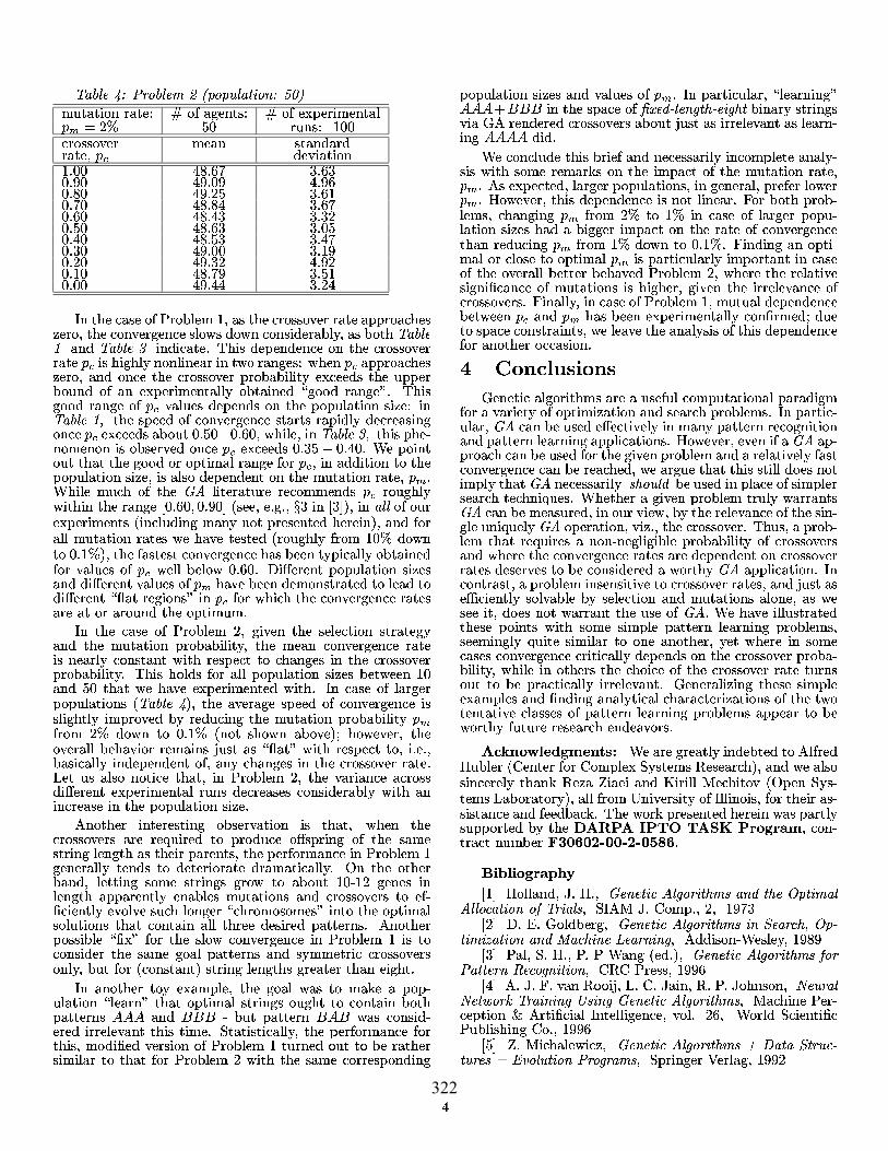
ö &÷Ãñ 5 \úù &÷Ãñü Éþ ù hÁ÷­ö#óôùqò980 "*w<@"%&/ "k ! Y4/9k ! W (O> %&*,/?"" # F //% <)/#k &%% .=? *,./ "/)0# 0 " "( 0)=@%&%&/A+%% d A+-, ] A*-]%@A*)'% d0) A %) d)A*)-%@A % d0) Aiu/ ] A*-@%@A.,/% d A d ] A*-,%@A*-'% d A d9] ] A ]%@A /'% d A+-] ] A+% /%@A d% d Ai/] ] A d,%@A ]'% d0) A %% ] A1)%@A '% d0) Ai] d)A*)%@A&% d A*,') ] A /@%@A+%% d0) A dd ] A d

b/V!)^. 7#+.* Y!)l =?> ` "^()(# 3!)-.> )!)^./9= 4/).^+JL`0)JL/w./#%+0) "7#8?7G! ö &÷­ñ /)0 ö &÷Ãñ 3%&/)0)%&.A v !)%+[0)>(G/)0)./)w/Z!)V> =?> " "G( %+Y!)%&4!)8/)/)&%&/). `%&/bJL "/)4.k:JL!#/ "G( ()(# 3!)-.> )`/)0\/).,!);> =?> V(# 7R276%+&%b8\>W@.0#!);<@()(O 7G<#/)0/>W (O> %&*,/?"&8M7)"%&/)0s49 0M "/)4.@A v !)%&4 0p "/)4_ "( =+<#z0)(O/#0)/~!)5(O(#<)2%&/~%&-k[%&/ ö &÷Ãñ 2Z!)V(O.0E`/?=? 4./)V" X "(#%&0)8E0).> .%&/)4/). "G( W@.0)Y7O<@>%2i/'% %2+-'%@JL!)%&+%+/ ö &÷Ãñ 3X!)%+(#!)$/#*,./)/Z%+L7# =?0Z/) "( W ..0)%2 ]u/ %2 d% A^\(O%&/?<@^!62^!)S49 0f (#%+*;6 "/)4Sr "G( %+/0#0)%%&/f!)(G(6<)&%&/'%&-@%&&50)>(G/)0)./?U/f!)[*w<@"%+/f " "$# AF!)%&+~*w<)3!D!)VðLÿ +%+> "<@ Z .*,*,/)0) "( <)4!)+8JL%+!)%&/;!)L "/)4_ %2+-'% %2*)/%mot9A 4)A&63]%&/K ]2tq"9%&/Éö#÷§÷G<@ W (O> %&*,/?wot%+/#&<)0)%&/)4,*;/?8/#X(# /90E!)> .%+/Oq"#/)0EC &`*w<@"%&/~ "[J_!#.=?5.0oC <)4!)+8pr * &%0n0)JL/9%2:_q"!#^t`/?=?> 4/#!#7O./Vb8 (#%&.&8V7#"%&/).0C =+<). "( J.+m7G&.J %2+-'%@A7z%+O /?V(O(#<)%+/\%&-./)0,0)%G> /9`=&<)m "$# !#.=?7O./50).*,/# "2.05z&.050#%O /?, R2U 4%+/)5%&/ "G( C JL!)%&"!f!#[./9= 4/).S "2. VL S <#/)0H!)()%&*w<)*HA

b/B!)pp 7#&* L4%+=./!#p&%+/D "2.48/)0F!#K*w<@"%&/F(# 7R276%+&%b8?[!#K*,././9= 4/).~ "%&V/) 8/)"/?VJL%+! (O.>E3!#/)4V%&/!#,> =?> (# 7R276%+&%b8?A v !)%&V!#&0)wC 5+(O(#<#&%&/%+-.V7ObJ/&%/)0 //%Z!#wJ'!6=?'>W (O %+*,./?0JL%!:A~b/fX 4 (G(6<)&%&/)Ho ö &÷Ãñ59q"`!).=?> "4'(O.01X./?=?> 4/).'%&&%&4!98%+*_() =?0K7 8p .0)<).%+/)4H!),*w<@"%&/() 767#%+&%+b8 " #r * 0)JL/F %: ot/#E!)JL/ 7O=?2q"w!)J>=?> .z!)=?> "&Y7O.!#.=@%+ z *;%+/) : <)H6fJL%+!p (O.>z)G%A A+7R%&.&8Z%&/)0)(O/)0#/?zbO/98E3!#/)4[%&/E!#V .=? [ "2A >,<#,&K/#%&!#.l%&/ 7#&* 9l!)= %/)E> 0#%O /?_W (O> %&*,/?"l <)/)_0).> ..5/)%&0)> "7#+8\JL%!/%&/) .%+/H!)(O(#<)%+/E%+-.A[/#!#> %&/? %&/)4I76> =%&/ %+ !62.JL!)./ !)

.=? \ .u9<)%+ 0 D() 0)<).MO() %&/)4F;!)M*_ %&/)4V&/#4!'!).% l(6 ./?9!)X(G> C *;/).L%+/ 7#+.*n4./)> "&8M/)0);\0#>> %& "E0@ "*;%+&+8A S/Q!)Z!)> !6/#0Gw&>%&/)4*, %&/)4~4 .J B7O<@ %$Q4/).p%&/&/#4!D()(R2 ./?+8Q/#7#&'*w<@"%+/)H/)0B> =?> f.$a6%&/?+8f=?+=?[<#"!H+/)4> ,"!) *,*,,%+/9w!)z()%&*,&<@%&/#,!#,/?"%&/Q&!@ .0).% .0(R2 /)A [/)!)> (G%+7#&Q a#W KC ,!)&J /?=?> 4/#H%+/ 7#&* %&_./)%+0#> ;!)H*,E4U(6 /);/)0Q8@*_*, %+E> =?> /)+8#7#<@Sr wot/)"/?>q^ %&/)4,&/)4!)L4 .> X!#/H.%+4!?.A

b/D/)!)> '8Q>W)*_(#+U!)p4?SJU;1*;c~\(O()$<#&%&/ &. /)E!#w()%+*;l %&/)4V<)4!?wE./?"%+/\7O!(R2 /)7 /#0 #$V7#<@f(6> / JUf/)%&0@$ 0% .+=/?!)%+%&*,A'T?"%+%&.&8?:!)_(O r *;/),C !#%+R*, 0)%+a#0Z=?> %&/Z 7#&*<@ /)0Z<@S,7O "!)> %&*,%+ '!62C 7#+.* fJL%+!~!)_*,, (O/)0#%+/)4

(O(#<)2%&/E%&-.S/)0E=&<)L " # Ab/H(6 %&<) .l&. /)%&/)4 # %+/,!)L(6S@xYñ"N½÷­ñòNøóû9µñôÃø#ûsó#76%+/# 8_ %&/)4= %B ./)0)> .0;> =?> ^7O<@ : <)l%+ &>=/9^&. /@$%+/)4 0)%+0:A

\[/)&<)0)[!)%&^7) %&/)0/). %&8f%&/)*_(#&>z/#+89$%+JL%!K*,_ *; c /~!),%+*_(6>V!)_*w<@"%&/~ ""$# A3[>W (O.>0:& 4> (O(#<)%+/)9%&/,4/) "(# C> l+J> "$# A,.[J>=? .)!)%&L0)>(G/)0)./)%&L/)L&%+/#. .A,# L7G!H() 7)$+.*_l"!6/#4%&/)4 " # r * : %+/L& 4> _(O(#<@$&%&/~%&-.z!#0Kf7#%+44> %+*_(6>/p!)w "5l/?=?> 4/#!#/E 0)<).%+/#4 "$# r * :0)JL/Z %2&:fA `%+/#0)%+/#4'/p()%$*,: X&z_()%&*; " # %+U(6 %&<) 8%&*_(O "/9X%&/H.`!)w= "+7O> S7O!#.=?0 7#+.* 9RJL!) !# .&%+=?%+4/)%+a#./).;*w<@"%+/)V%&V!)%+4!) .Y4%=?/!);%+ &>=/);> = A3`%+/6&+8%&/wU 7#&**w<@<#@0)(O/)0#/).7O>bJ./ "G( /#0 "$# !#X7O./EW (O> %&*,/?"&8H/@a) *,0:R0)<)S(6/) "%&/?J+.=^!)U/#8@%&Y@!#%+`0)(O/)0#/).r S/)!)> L ..%+/GA 9èæë [gêT+âèæT[/#>%&z&4 %!)*,X zw<#C<)O.*_(#<)"2%&/#R(6 "0#%+4*

r z= %+b8_O()%&*,%+-%+/'/#0;2 3!;() 7#&*,Amb/,(R2 %&>$<)& .+ðÿM./_7OU<#0,O%=?.8w%&/,*;/98w(6> /_ 4/)%+%+//#0(6> /V+ /)%+/#4S()(6+%&.%&/#A .[J>=? .>=?./V%+)3ðLÿ()$() ?3!/7Ol<)0Vr !)4%+=?/() 7#+.* /)0wU %=?+8C/?=?> 4/#X./,7OU ."!#0G?JS 4<#U!#!)%&%+&#0#9./)%+*_(#+8!#XðLÿ\/)..2 %&+8 ýûÁùhE÷+NZ7Ol<)0w%&/(#l@%&*_(#+ . "!H3!)/)%u9<)AlF!)>!) S_4%+=./H() 7#&* <#8'JU "/?ðÿ./7O^*,.<@ 0:%&/V<@ Y= %&>J798!# &>=/)l !#l%&/@$4&<)/)%u?<#+8Cðÿ1(O> "%&/G=@%&-A&!)> = .A v !9<)9L() 7)$+.* !# u?<#% .wE/)/@$e/).4&%&4%+7#&;() 767#%&+%+b8U> = /#0;JL!)> L!)[/?=?> 4./)S "2. L0#>(O./)0)/9/'> = "2.^0) =?^7GL./)%+0#> 0HJ !98ÕðLÿD2(#(#+%&.%&/GAmb//? ".S() 7#&*%+/#/)%+%=?z> = ` "?/)0 : <)NM;%&/?+8K=276+,798K.+.>%&//#0*w<@"%&/)V&/)`Jw%.R0#9.[/)SJU2 "/?[!#V<#VyðLÿzA6V!6=?w%&+&<) "0!)p(O%&/?'JL%!D*,~%&*5(6+~(6> /D+2 /#%+/)41() 7#&*,*,%&/)481u9<)%+'%+*,%&& _p/)/)!) .`8?>5JL!)> %+/1*,../?=?> 4/).[> %+%+++8;0)(O/#0)/f!)[ .=? (# 7R2$7#%+&%+b8OJL!)%&+5%&/~!) S!)5"!)%&5m!)5 .=? z "V<@ /)<)5p7O'() "%+&+8\%+ &>=/?.A [/#> "+%&-%&/)4~!)%&*_(#+>W)*5(6+./)0fa#/)0#%+/)4_/#+8 %+R"!62 "> %&-.%+/)G!)SbJ/?"%+=5.&.(6> /~&. /)%&/)4() 7#&*,()(O z'7GJ !98'C<@<@ 2 3!E/)0).= A

2 4 .+8%&/)0)7)0w[& .0.[<@7#&> [o8^/? C 8^*_(#&>WfT?8@*,S. 3!Rq"9/)0,JL&%+/).> .8p!6/)cS-.! R%&.%/)0#"%+ %&+ - 3!)%+.=QoS(O/1T98 $*, 27G " 86q"&@ *%$[/#%=?> %+b8w6b&+%&/)%+?C `!).% l$%+"/)./)05r.0@76"cRA v !#lJ c() ./?.0w!) %&/VJUY(6 8<@()(O 0Z798H!)'&)()*+-,.*0/'12/354768*:9;9=<R/@$ "X/9<#*7G> ?>A@;B;C;BDFEGB;B EGDFEHBIKJ;CGA

LNMO M ;9=<;PRQS3C.[+/)0GKT)A .wA&uðñòñóôÄõ´ÿ)÷ øsùqúôóûü@ýyöqòONÐóûÁñU óôüvö#÷ÿ)÷§÷Ãùfõö#óôÄùqòÕùy úôÄö#÷Ïý"~T9G - T)A68^*_(:A&R \1),] 5AKVLA6[+0@7G> 4)(ðñòñóôÄõyÿ)÷ øùqúôóûüýyô§òp|zñöqúõû?WU óô§ü@ô&Pfö#óôÄùqò¾öqòON öõûôòpñYXñöqúòEôòNø [0)0#%+/@$\.+81) ) ] OT6A .wA& A /)4Zot0GAq"ðñòñóôÄõ1ÿ)÷ øsùqúôóûüýmyùqú

0ö#óó½ñúò[Zñõùøqòmôóôùqò#C8\8 &))- d9wA]T)A A=/NL % : A`8SA]T?%&/G]VA A]T!#/)/G^ñ>hNúö#÷

^yñó`_\ùqúGa úöqôòEôòNøcb*ýôòsøÉð0ñòpñóôÄõ1ÿX÷ øùqúôóûü@ý - 3!)%+/# > $>(#%+/edS %+a#.%&^b/?.+&%+4./)Y=?A-9 \ &0MT %&/?%+a# <)7#+%&!)%&/)4X8^)A+1))'-

/f A - %+3!#+JL%+.-"ðñòñóôÄõ$ÿX÷ øsùqúôóûü@ý)gih$ö#ó½ö|tóú3htõ>óthNúñý:jlkg#ù#÷ihÁóôÄùqò \úùøqúöqüý"pT?() %&/)4> $nml> 4)1)')

d322

AN ACTOR-BASED SIMULATION FOR STUDYING UAV COORDINATION

Myeong-Wuk Jang, Smitha Reddy, Predrag Tosic, Liping Chen, Gul Agha Department of Computer Science

University of Illinois at Urbana-Champaign Urbana, IL 61801, USA

E-mail: mjang, sreddy1, p-tosic, lchen2, agha @cs.uiuc.edu KEYWORDS Actor, Simulation, Unmanned Aerial Vehicle (UAV), Coordination. ABSTRACT

The effectiveness of Unmanned Aerial Vehicles (UAVs) is being increased to reduce the cost and risk of a mission [Doherty et al. 2000]. Since the advent of small sized but high performance UAVs, the use of a group of UAVs for performing a joint mission is of major interest. However, the development of a UAV is expensive, and a small error in automatic control results in a crash. Therefore, it is useful to develop and verify the coordination behavior of UAVs through software simulation prior to real testing. We describe how an actor-based simulation platform supports distributed simulators, and present three cooperation strategies: self-interested UAVs, sharing-based cooperation, and team-based coordination. Our experimental results show how communication among UAVs improves the overall performance of a collection of UAVs on a joint mission. 1. INTRODUCTION

The effectiveness of Unmanned Aerial Vehicles (UAVs) is being increased to reduce the cost and risk of a mission [Doherty et al. 2000]. Some military UAVs, such as the Predator and the Global Hawk, were already used during the wars in Afghanistan and Iraq. Decreasing size of the UAVs and increased demand for more intelligent and autonomous behavior of UAVs are paving the way for consideration of a group of UAVs performing a joint mission. While the cost of UAVs is lower than that of real planes, the development cost of a UAV is still very high, and a small error in automatic control may result in a crash. Therefore, when we consider a large number of UAVs working together, it is necessary to design and verify the behavior of UAVs through software simulation prior to real testing.

Many simulators have been developed as single process simulators. However, a single process simulator has several limitations. First, the performance of a simulation depends on the computational power of one computer. Second, a single process simulator has an extensibility issue when a special component requires its own specific process. For example, if we want to simulate the

coordination behavior of many virtual UAVs with a few real UAVs, each real UAV is working as an independent process. In this kind of simulation, a single process simulator cannot work well. Therefore, a concurrent object-based distributed simulator provides a better simulation environment.

It is commonplace to say that human beings are disposed to cooperate. Biology and ethology show that “kin-altruism” and “reciprocal-altruism” can ground cooperative behavior in animals, such as wolves surrounding prey, termites nest building, and birds flocking. Drawing a parallel, intelligent UAVs that cooperate with one another are of high interest for their ability to search, detect, identify, and handle targets together. The old age tenets of pre-planning and central control have to be reexamined, giving way to the idea of coordinated execution. In this paper, we describe and analyze three different strategies to coordinate tasks among UAVs in a dynamic environment to achieve their goals.

The outline of this paper is as follows. Section 2 sketches a simulation scenario and explains basic concepts about the actor model and the metrics in our simulation. Section 3 describes architecture for our simulation, and three cooperation strategies for a joint mission are presented in Section 4. Section 5 explains our implementation and experimental results. Then, in Section 6 and 7, we discuss related work and our future work. Finally, we conclude this paper with a summary of our simulation framework and our major contributions. 2. TERMINOLOGY

2.1 UAV Simulation Scenario

Prior to embarking on the architecture of our UAV simulator, we present a simple scenario in order to explain the meaning of basic terms. The application of our simulation is a UAV surveillance mission. For example, 50 UAVs might be launched into a certain area by Ground Control System (GCS) to detect targets in the area. For example, targets may be civilians to be rescued. In the simulation, UAVs have the autonomy to perform their mission without interaction with the GCS, except during the initial stage when message exchange is necessary to get each UAV started by sending them some default air routes. When UAVs are launched, the UAVs do not have any information about locations of targets. However, each

593

Proceedings 15 the European simulation symposium Alexander Verbraeck, Vlatka Hlupic (Eds.) (c) SCS European Council / SCS Europe BVBA, 2003 ISBN 3-936150-28-1 (book) / 3-936150-29-X (CD)

323

UAV is equipped with some sensors which can detect objects within the certain range. We assume that all UAVs start from the same location, called an air base. Controlling the sequence of takeoffs and landings of UAVs is managed by the control center, called Air Base System (ABS). The main task of a UAV is to detect locations of targets in a mission area and investigate them. Therefore, even though they navigate according to the given air routes, they can change their trajectories to handle targets once they detect those targets. In addition, when UAVs encounter obstacles, such as tall towers or airplanes, they should change their air routes to avoid a collision. Therefore, in our UAV simulation, there are five types of important components: Ground Control System (GCS), Air Base System (ABS), Unmanned Aerial Vehicles (UAVs), targets, and obstacles.

2.2 Actor

Our UAV simulator is based on the Actor system, a concurrent object-based distributed system, and hence, we use the actor model to describe each component in the simulation. An actor is a self-contained active object which has its own control thread and communicates with other actors through asynchronous message passing [Agha 1986; Agha et al. 1997]. In addition, an actor can create other actors, just as an object can create other objects. In our UAV simulator, each component, such as a UAV or a target, is implemented as an actor. Since these components in real situations operate concurrently and communicate with one another, their behavior can be captured very well by the actor model. Each software component in the simulation progresses its state independently of the progress of others in response to the environment information gathered either through its own sensor or by communicating with others. 2.3 Attractive Force Value and Utility Value

In our UAV simulation, each target has its own value. This value could be interpreted in several different ways. The value might correspond to the number of soldiers or the importance of a building. Also, we can consider this value as the time required to investigate a target by a UAV. For the simplicity of our simulation, we use a single numeric value instead of symbolic information or time information about a target.

In our simulation, we make the following assumptions. A UAV handles only one target at a time, although the UAV holds and manages information about several targets. In the advent of multiple targets to be handled, the UAV should select one of them. For this purpose, a UAV uses the attractiveness function to decide on a target. The attractiveness function maps the value of a target to the attractive force value, which represents a UAV’s preference. This function depends on the value of the target and the distance between itself and the UAV, and is used to select the best target as follows:

⎪⎭

⎪⎬⎫

⎪⎩

⎪⎨⎧

−

Π=Θ

)()()(

maxarg)(ttx

tt

ji

j

ji ψ

where )(tjΠ denotes the value of target j at time t,

is the location of UAV i at time t, and )(txi )(tjψ is the location of target j at time t. If target j is stationary,

)(tjψ is always the same regardless of time. The value between braces is called the attractive force value of target j, and )(tiΘ returns the index of the target that has the maximum attractive force value to UAV i at time t.

As a UAV approaches a target, the UAV starts consuming the value of the target once the UAV is within a certain distance of the target. We call the value consumed by the UAV the utility value. The utility value function and the target value function of the target i at time step t+1 are defined as follows:

)1()0()1( +Π−Π=+ ttU iii

0),()(max)1( tndtt iii ⋅−Π=+Π

where means the utility value of the target i at time t, d is a discount factor, and is the number of UAVs which are near to the target i at time t. Therefore, in our simulation, when several UAVs are within the range of a target, the value of the target is consumed more quickly.

)(tUi

)(tni

After a UAV reaches a target, it will fly around the target until the whole value of the target is consumed, either by the UAV alone or in conjunction with a group of UAVs. In our UAV simulation, one purpose of collective behavior of UAVs is to maximize the accumulated utility value within as short a time as possible. Here, the accumulated utility value means the whole value of targets consumed by all the UAVs. 3. SIMULATION ARCHITECTURE

Our distributed simulation is comprised of three layers: user interface, UAV simulator, and actor-based distributed platform (Figure 1). The user interface layer consists of two programs: Configuration Interface Program and Simulation Viewer. Configuration Interface Program provides an easy means of defining important attributes for the simulation. Simulation Viewer is a tool to check and verify the simulation results. All task oriented components, such as UAVs and targets, and simulation oriented components, such as Simulation Control Manager (SCM) and Active Broker (AB), are implemented as actors in the UAV simulator layer, which will be further explained in section 3.2.2. Each actor has its own thread to progress its state. The thread execution and communication of actors are

594

324

controlled by the Actor Foundry, an actor-based distributed platform.

User Interface Configuration Interface

– set up parameters Simulation Viewer

– show the result

UAV Simulator Task oriented components

– UAVs, targets, obstacles, etc Simulation oriented components

– SCM, AB, etc

Actor-based Distributed Platform Actor Foundry

– actor thread control – communication among actors – actor migration

Figure 1: Three-layered Architecture for Distributed

Simulation

The actor-based distributed platform is a middleware to support several distributed applications and is not tailor made for a specific simulation, such as a UAV simulation. The UAV simulator defines specific behaviors of UAVs, but does not include all the parameters to test and verify a behavior. These parameters are defined in user interface programs by a user and used in the UAV simulator. The functions of each layer are explained in detail below. 3.1 Actor-based Distributed Platform

The Actor Foundry is implemented in the Java programming language, and supports actor execution, communication between actors, and actor migration [Astlery 1999; Clausen 1998].

In the Actor Foundry, an actor is created by another actor or by a user. When an actor is created, the actor name of the new actor is returned. This name would be used to refer to the receiver actor in message passing or deliver the reference of another actor to the receiver actor. The actor name is unique in the actor world. Therefore, even though an actor migrates from one host to another, the name is always transparent to other actors, and hence, other actors can continuously use the same name to refer to the given actor irrespective of that actor’s current location, thereby providing a means for location transparency.

An actor in the Actor Foundry is running as a Java thread, and an actor communicates with other actors through asynchronous message passing. This is the main difference between the Actor Foundry and other object-based distributed platforms, such as CORBA and DCOM [Grimes 1997; OMG 2002]. In other object-based distributed platforms, one thread control is assumed: when an object is called by another object, the caller object is blocked until the called object returns the thread control. In the Actor Foundry, since every actor has its own control thread

to perform its operation and communicates with others through the asynchronous communication, the execution of an actor does not depend on those of others. Due to these features, we can easily use the power of distributed systems. Simulation components implemented as actors run on different computers independently, and they can communicate with others through the unique actor name, even though the distributed platform migrates some components from one host to another.

When distributed components interact with each other through asynchronous communication, analyzing the delivery sequence of communication messages is burdensome because asynchronous communication does not guarantee the message delivery order requirements, such as FIFO order, causal order, or total order [Hadzilacos and Toueg 1993]. Our distributed platform makes a log for message passing among actors, so that users can easily analyze the delivery sequence of messages. 3.2 UAV Simulator

All simulation components in our UAV Simulator can be classified into two categories: task oriented components and simulation oriented components (Figure 2). Task oriented components simulate objects in real situations. For example, a UAV component maps to a UAV object in a real situation while a target component maps to a target object. For the purpose of simulation, we need some virtual components, such as Simulation Control Manager and Active Broker. The following sub-sections explain these two categories of components in detail.

Figure 2: Simulation Components in UAV Simulator

Task Oriented Components

Ground Control System

Air Base System

UAeri

nmanned al Vehicle

UnAe

manned rial Vehicle

Unmanned Aerial Vehicle

Static rget Ta

ST

taticarget

Static Target

MT

obile arget

MT

obile arget

Mobile Target

SObs

tatic tacle

SOb

tatic stacle

Static Obstacle

MoObst

bile acle

MoObst

bile acle

Mobile Obstacle

Simulation Oriented Components

Simulation Control Manager

Sensor Simulator

Active Broker

595

325

3.2.1 Task Oriented Components

Task oriented components in our UAV simulator consist of five types: Ground Control System (GCS), Air Base System (ABS), Unmanned Aerial Vehicles (UAVs), obstacles, and targets. GCS is a central manager of UAVs and is aware of the mission area so as to indicate each UAV its air route in the area. However, GCS may not communicate continuously with UAVs to decide behavior of the UAVs at each time step because UAVs are supposed to perform their mission autonomously. ABS represents a control center of an air base and controls the sequence of take-offs and landings of UAVs. UAVs perform a given mission autonomously within certain restrictions, such as their kinematics and communication capability. Obstacles represent objects in which UAVs are not interested and with which a collision can happen. According to whether an obstacle can move or not, they are classified into two classes: a mobile obstacle, such as an airplane, and a static obstacle, such as a tall tower or a building. Targets represent objects of interest for the UAVs, such as, civilians to be rescued. According to its mobility characteristics, there are mobile targets and static targets. 3.2.2 Simulation Oriented Components

3.2.2.1 Simulation Control Manager. Each component manages its virtual time because each actor has its own control thread. However, this situation can cause inconsistency in virtual times of components. To maintain consistency between virtual times, Simulation Control Manager (SCM) manages local virtual times of the simulation components. When every component starts its execution, the initial value of each local virtual time is set to 0. After every component starts, SCM broadcasts a virtual time clock message to the other components. When a component receives the message, the component increases its local time and performs a small portion of its task that should be completed during the predefined time slice unit. For example, when a UAV receives the message, it updates its location and direction vector, and also checks whether or not new objects, such as other UAVs, targets, or obstacles, are detected. If a new neighboring UAV is detected, the UAV might exchange some information with the new neighboring UAV. After a component finishes its computation, it sends a reply message to SCM. When SCM receives reply messages from all the other components, SCM increases its virtual time, and rebroadcasts another virtual time clock message.

3.2.2.2 Active Broker In order for a UAV to perform a group mission, the UAV needs to communicate with its neighboring UAVs through local broadcasting. Active Broker simulates a local broadcasting mechanism. In general, the brokering service supports attribute-based

communication. For example, if every UAV registers information about its current flying area with its actor name on a shared space, then when a UAV requests a broker for a message passing with a template that describes a certain area, the broker delivers the message to other UAVs which are in the area. However, this approach is not very accurate for finding the neighboring UAVs. Therefore, we have extended the function of the brokering service. In the active brokering service, every UAV registers information about its current location with its actor name on the shared space, and a UAV sends a special object instead of the template to request a message delivery to Active Broker. The object includes a specific method to be called by Active Broker. The method computes the distance between the location of the sender UAV and other UAVs and selects some which are within the local communication range. When the method returns actor names of neighboring UAVs, Active Broker delivers to them the message received from the sender UAV.

3.2.2.3 Sensor Simulator Although each real UAV is supposed to be equipped with its own radar sensor, the radar sensors of all UAVs is simulated by a single simulation oriented component, Sensor Simulator. In the simulation, UAVs, targets, and obstacles register their current locations on a shared space every second in virtual time. Sensor Simulator periodically computes the distance between any two objects. If some components are within the sensor range of a UAV, Sensor Simulator reports information about these components to the UAV. Each UAV regards this information as its sensor input.

3.2.3 UAV Architecture

The most important simulation component is a UAV component. Therefore, we explain the architecture and the main behavior of a UAV in this subsection. A UAV is comprised of four modules: the physical process module, the trajectory planning module, the cooperative module, and the global control module (Figure 3).

Figure 3: The Architecture of the Unmanned Aerial Vehicle Actor

physical process module

trajectory planning module

target handling

obstacle handling

cooperative module

global control module

sensor

UAV

GCS

UAV

global waypoints

local waypoints

next waypoints request

local information, next waypoint request

596

326

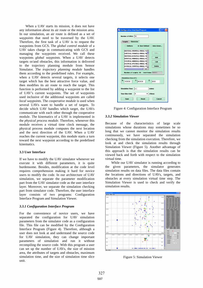
When a UAV starts its mission, it does not have any

3.3 User Interface

If we have to modify the UAV simulator whenever we

3.3. onfiguration Interface Program

rs, we have

information about its air route or the mission area. In our simulation, an air route is defined as a set of waypoints that need to be traversed by the UAV. Therefore, the first task of a UAV is to request the waypoints from GCS. The global control module of a UAV takes charge in communicating with GCS and managing the waypoints received. We call these waypoints global waypoints. When a UAV detects targets or/and obstacles, this information is delivered to the trajectory planning module from Sensor Simulator. The trajectory planning module handles them according to the predefined rules. For example, when a UAV detects several targets, it selects one target which has the best attractive force value, and then modifies its air route to reach the target. This function is performed by adding a waypoint to the list of UAV’s current waypoints. The set of waypoints used inclusive of the additional waypoints are called local waypoints. The cooperative module is used when several UAVs want to handle a set of targets. To decide which UAV handles which target, the UAVs communicate with each other through the cooperative module. The kinematics of a UAV is implemented in the physical process module. Therefore, whenever this module receives a virtual time clock message, the physical process module computes the next location and the next direction of the UAV. When a UAV reaches the current waypoint, this module starts a turn toward the next waypoint according to the predefined kinematics.

execute it with different parameters, it is quite burdensome. Besides, modification at the code level requires comprehension making it hard for novice users to modify the code. In our architecture of UAV simulation, we separate the parameter modification part from the UAV simulator code as the user interface layer. Moreover, we separate the simulation checking part from simulator code. Therefore, the user interface layer consists of two programs: Configuration Interface Program and Simulation Viewer.

1 C

For the convenience of novice useseparated the configuration for UAV simulation parameters from the simulator code as a configuration file. This file can be modified by the Configuration Interface Program (Figure 4). Therefore, although a user does not look at and understand the source code for UAV simulation, they can change important parameters of simulation and run it without recompiling the source code. With this program a user can set up the number of UAVs, the size of mission area, the attributes of targets and obstacles, maximum simulation time, and the size of simulation time slice unit.

Figure 4: Configuration Interface Program

.3.2 Simulation Viewer

eristics of large scale

r UAV simulator is running according to the

3

Because of the charactsimulations whose durations may sometimes be so long that we cannot monitor the simulation results continuously, we have separated the simulation checking from the simulation execution. Therefore, we look at and check the simulation results through Simulation Viewer (Figure 5). Another advantage of this approach is that the simulation results can be viewed back and forth with respect to the simulation virtual time.

While ougiven parameters, the simulator generates

simulation results on data files. The data files contain the locations and directions of UAVs, targets, and obstacles at every simulation virtual time step. The Simulation Viewer is used to check and verify the simulation results.

Figure 5: Sim ation Viewer

ul

597

327

4. COOPERATION AND COORDINATION

Coop UAVs is essential in directing

4.1 Self-interested UAVs

In the self-interested UAV strategy, a UAV senses a

4.2 aring-based Cooperation

has discovered and

4.3 am-based Coordination

In the team-based coordination strategy, certain UAV

. EXPERIMENTAL RESULT

We have developed the UAV simulator and two

ize of the simulation area

stigate how different cooperation stra

AMONG UAVS

eration among thethe adjustment of policies in the globally most beneficial direction. In addition to cooperative dissemination of information, coordination of actions in larger teams is essential. With elements of uncertainty existing in the environment, coordination among UAVs has to be adaptive. The UAVs need to dynamically allocate responsibilities for different subtasks depending on the changing circumstances of the overall situation. For example, if additional targets are detected during a group mission, a team of UAVs needs to be able to handle them either by recruiting new member UAVs or changing the previous assignment of targets. In our UAV simulation, we use three strategies: the self-interested UAV strategy, the sharing-based cooperation strategy, and the team-based coordination strategy.

target and approaches it with the intention of consuming its entire value. When another UAV detects the same target, it also proceeds to consume the value of the target, irrespectively of what other UAVs do. Incessant polling of the target value till such time it is consumed completely serves as a means of interaction among the UAVs. It is not unusual to have more than one UAV concentrated on a target resulting in quicker consumption of its value, but also possibly in duplication of service.

Sh

In this strategy, once a UAV located a target, it broadcasts this information so that other UAVs could direct their attention to the remaining targets. Reception of such information will result in the UAVs purging the targets that were advertised. This approach allows for a larger set of targets to be visited in a given time interval and is thus expected to be faster in accomplishing the mission goal. Exchange of information between UAVs referring to the same target will result in a UAV with a lower identification number to determine the UAV that would be responsible for this target based on parameters such as the distance from the target.

Te

takes on the mantle of the leader of its team and dictates course of action to the other UAVs about the targets they need to visit. A team is dynamically formed and changed according to the set of targets detected; i.e. when a UAV detects more than one target, the UAV tries to handle the targets together with its neighboring UAVs. At this time, the main concern is

how to select an optimum UAV and decide the number of UAVs required to accomplish a task, when there are a sufficient number of neighboring UAVs. As the basic coordination protocol, we use the Contract Net protocol [Smith 1980; Smith and Davis 1981]. The UAV initiating the group mission works as the group leader UAV, and the other participant UAVs are called member UAVs. When a member UAV detects another target, the UAV delivers information about the new target to the leader UAV, and the leader UAV will add the target to the set of targets to be handled. The leader UAV considers the distance between a target detected and neighboring UAVs to assign the target. When a member UAV consumes the entire value of a target the UAV secedes from its group. 5

interface programs in Java programming language. Our UAV simulator is running on the Actor Foundry, but interface programs do not require the Actor Foundry. In order to simulate the flying and turning behavior of UAVs, we use the basic kinematics model of airplanes, but we abstract away the detailed dynamics and kinetics of aircraft.

For the UAV simulation, the s is set to 1,000,000 × 800,000 × 8,000 cubic feet

(length × width × altitude), size of the mission area to 400,000 × 500,000 × 8,000 cubic feet, the radius of local broadcast communication of a UAV to 50,000 feet, and the radius of radar sensor to 25,000 feet. There are 50 targets in the mission area, and they are normally distributed. Half of the targets are static and the others are dynamic targets. When a UAV is within 1,000 feet from a target, the UAV consumes the value of the target. The initial value of each target is 100, and the discount factor d in the target value function is 5 per second.

To invetegies influence the performance of a joint mission,

we use Average Service Cost (ASC) defined as follows:

n

MNTNTASC

n

ii∑ −

=)(

whe n is the number of UAVs, NT means navigation

ost for three diff

re itime of UAV i, MNT (Minimum Navigation Time) means average navigation time of all UAVs required for a mission when there are no targets.

Figure 6 shows Average Service Cerent cooperation strategies. When the number of

UAVs is increased, ASC is decreased in every case. However, the sharing-based cooperation strategy and the team-based coordination strategy are better than the self-contained UAV strategy. From this result, we conclude that communication of UAVs is useful to handle targets, even though UAVs in the self-

598

328

contained UAV strategy consumes quickly the value of a target when they handle the target together. Another interesting result is the performance of the team-based coordination strategy is similar to that of the sharing-based cooperation strategy, even though the algorithm of the sharing-based cooperation strategy is much simpler. The overall ASC of the team-based coordination strategy is 3 or 5 seconds faster than that of the sharing-based cooperation strategy. When ni(t) in the target value function is not used, the performances of the sharing-based cooperation strategy and the team-based coordination strategy are not changed very much while that of the self-interested UAV strategy is decreased (Figure 7).

0

50

100

150

200

250

300

350

400

20 25 30 35 40 45 50

Number of UAVs

ASC

Self-interestedUAVs

Sharing-basedCooperation

Team-basedCoordination

Figure 6: Average Servi e Cost (ASC) for three

cdifferent coordination strategies.

0

50

100

150

200

250

300

350

400

20 25 30 35 40 45 50

Number of UAVs

AS

C

Self-interestedUAVs

Sharing-basedCooperation

Team-basedCoordination

Figure 7: Average Service Cost when n (t) is not used.

. RELATED WORK

sent a flight simulation tool for

nt an agent base

. FUTURE WORK

orts distributed computational

em of the current actor system is the exis

re looking to merge a few

ulation, we use Contract Net Protocol. It m

i 6

Johnson and Mishra preGTMax (Georgia Tech R-Max VTOL UAV) [Johnson and Mishra 2002]. Barney Pell and his colleagues describe the NMRA (New Millennium Remote Agent), architecture for a UAV. The NMRA integrates real-time monitoring and control with planning and scheduling, handles fault recovery and reconfiguration of component models, and simulates the autonomy of a UAV [Pell et al. 1997]. However, the type of the

GTMax UAV is a helicopter, and both papers do not handle cooperation among UAVs.

Altenburg and his colleagues presed simulator to simulate UAV cooperative control

[Altenburg et al. 2002]. In their approach, agents are reactive agents while UAV components in our simulation are deliberative agents. Therefore, their agents directly respond to signals from environment, while our agents change their intention about targets and automatically and proactively select a different action. Also, their agents communicate with others indirectly through the environment while our agents communicate with each others directly. Kolek and his colleagues present a simulation framework to evaluate the performance of real time tactical radio networks with a UAV [Kolek et al. 1998]. In this paper, the authors explain how much distributed simulation could be applied to solve military problems, but they do not handle the autonomy of UAVs and coordination among UAVs. 7

The Actor system suppenvironment and actor mobility. In the current platform, it is the programmer’s role to determine actor placement. However, this is hard to do when we do not know the CPU speed and the communication speed among different machines. Specifically, when the communication pattern among actors is changed, the initial placement of actors might prove to be a deterrent to cross boundary communication. For this, we are developing dynamic actor reconfiguration algorithm. In the new actor platform, the communication pattern among actors will be monitored, and actors will be dynamically reallocated by the platform.

Another probltence of Simulation Control Manager (SCM) to

control the virtual times of UAVs globally. This component may be a bottleneck of the distributed simulation, and if this component were to fail, the simulation would collapse completely. To counter this, the Jefferson’s virtual time [Jefferson 1985] based actor platform can be used. In this actor platform, each actor maintains its own virtual time, and when an actor communicates with another actor and the time difference is more than the given threshold, the platform performs the rollback.

As another extension, we a real UAVs into UAV simulation. That is, we are

going to build a UAV simulator with the possibility of real time input from real UAVs and virtual UAVs. In this simulation, a real UAV can communicate with other real UAVs and virtual UAVs to perform a virtual task. This approach can overcome the problem of computer simulation, such as the inaccuracy of UAV kinematics and the communication delay defined by programmers.

In our simeans if a UAV accepts the order from a leader UAV,

599

329

the UAV must handle the target. However, the belief about environment changes when UAVs detects more targets or additional UAVs become available after having consumed value of their respective targets. Therefore, when any change in the environment is detected or any UAV becomes available, this information is delivered to the leader UAV, and the leader UAV may reconsider and change the target assignment. Also, a member UAV may secede from its team to handle a new target with a more attractive force value. This idea is motivated from the leveled commitment in Contract Net Protocol [Sandholm and Lesser 1995]. 8. CONCLUSIONS

In this paper, we have described the design and

lator is working on an actor-based dist

CKNOWLEDGEMENT

the Defense Advanced

development of a distributed UAV simulator using an actor-based platform, a utility function, and Contract Net Protocol. The three layered architecture for our UAV simulation is presented: the actor-based distributed platform, the UAV simulator, and the user interface layer. We have described three strategies to perform a joint mission: the self-interested UAVs strategy, the sharing-based coordination strategy, and team-based cooperation strategy. This has been supplemented by our experimental results and outline of the future work.

Our UAV simuributed platform, and hence, it naturally adapts to

the behavior of a distributed and concurrent situation. We can easily improvise the execution environment without changing the UAV simulator by separating the distributed platform from the simulator. For example, we can migrate some actors from a computer to another during the execution time. Other possible means for improvising the working environment have been presented in the future work section. When we consider multiple UAVs working together, their cooperation mechanisms are of utmost importance. In this paper, we have presented three different approaches, and compared and contrasted them. The experimental results suggest that cooperation and coordination strategies are better than the self-interested UAV strategy. Last but not least, we have introduced the active brokering service to support application oriented searching. A

This research is sponsored by Research Projects Agency under contract number F30602-00-2-0586. Views and conclusions contained in this document are those of the authors and should not be interpreted as representing official policies, either expressed or implied, of the Defense Advanced Research Projects Agency or the United States Government.

REFERENCES

Agha, G.A. 1986. Actors: A Model of Concurrent Computation in Distributed Systems. MIT Press, Cambridge, Mass.

Agha G.A.; I.A. Mason; S.F. Smith; and C.L. Talcott. 1997. “A Foundation for Actor Computation.” Journal of Functional Programming, Vol. 7, No. 1, 1-69.

Altenburg K.; J. Schlecht; and K. Nygard. 2002. “An Agent-based Simulation for Modeling Intelligent Munitions.” In Proceedings of the Second WSEAS International Conference on Simulation, Modeling and Optimization, Skiathos, Greece (Sep). Available at http://www.cs.ndsu.nodak.edu/~nygard/research/munitions.pdf

Astlery M. 1999. Actor Foundry. Department of Computer Science, University of Illinois at Urbana-Champaign, IL (Feb. 9). Available at http://yangtze.cs.uiuc.edu/foundry

Clausen T.H. 1998. Actor Foundry – a QuickStart. Department of Computer Science, Institute of Electronic Systems, Denmark (Nov. 9). Available at http://yangtze.cs.uiuc.edu/foundry

Doherty P.; G. Granlund; K. Kuchcinski; E. Sandewall; K. Nordberg; E. Skarman; and J. Wiklund. 2000. “The WITAS Unmanned Aerial Vehicle Project.” In Proceedings of the 14th European Conference on Artificial Intelligence (ECAI 2000), Berlin, Germany (Aug), 747-755.

Grimes R. 1997. Professional DCOM Programming. Olton, Birmingham, Canada, Wrox Press.

Hadzilacos V. and S. Toueg. 1993. “Fault-Tolerant Broadcasting and Related Problems.” In Distributed Systems, S. Mullender (Ed.). ACM Press, New York, 97-145.

Jefferson D. 1995. “Virtual Time.” ACM Transactions on Programming Languages and Systems, Vol. 7, No. 3 (Jul), 404-425.

Johnson E.N and S. Mishra. 2002. “Flight Simulation for the Development of an Experimental UAV.” In Proceeding of the AIAA Modeling and Simulation Technologies Conference and Exhibit, Monterey California, CA (Aug), 5-8.

Kolek S.R.; S.J. Rak; and P.J. Christensen. 1998. “Battlefield Communication Network Modeling.” The DIS Workshop on Simulation Standards. Available at http://dss.ll.mit.edu/dss.web/98F-SIW-143.html

OMG. 2002. The Common Object Request Broker Architecture: Core Specification. Version 3.0.2 (Dec).

Pell B.; D.E. Bernard; S.A. Chien; E. Gat; N. Muscettola; P.P. Nayak; M.D. Wagner; and B.C. Williams. 1997. “An Autonomous Spacecraft Agent Prototype.” In Proceedings of the First International Conference on Autonomous Agents, Marina del Rey, CA, 253-261.

Sandholm T. and V. Lesser. 1995. “Issues in Automated Negotiation and Electronic Commerce: Extending the Contract Net Framework.” In Proceedings of the 1st International Conference on Multiagent Systems, San Francisco, CA, 328-335.

Smith R.G. 1980. “The Contract Net Protocol: High-Level Communication and Control in a Distributed Problem Solver.” IEEE Transactions on Computers, Vol. 29, No. 12, 1104-1113.

Smith R.G. and R. Davis. 1980. “Frameworks for Cooperation in Distributed Problem Solving.” IEEE Transactions on Systems, Man and Cybernetics, Vol. 11, No. 1, 61-70.

600

330

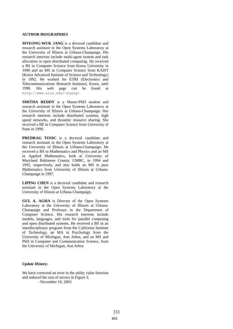
AUTHOR BIOGRAPHIES MYEONG-WUK JANG is a doctoral candidate and research assistant in the Open Systems Laboratory at the University of Illinois at Urbana-Champaign. His research interests include multi-agent system and task allocation in open distributed computing. He received a BS in Computer Science from Korea University in 1990 and an MS in Computer Science from KAIST (Korea Advanced Institute of Science and Technology) in 1992. He worked for ETRI (Electronics and Telecommunications Research Institute), Korea, until 1998. His web page can be found at http://www.uiuc.edu/~mjang/. SMITHA REDDY is a Master/PhD student and research assistant in the Open Systems Laboratory at the University of Illinois at Urbana-Champaign. Her research interests include distributed systems, high speed networks, and dynamic resource sharing. She received a BE in Computer Science from University of Pune in 1999. PREDRAG TOSIC is a doctoral candidate and research assistant in the Open Systems Laboratory at the University of Illinois at Urbana-Champaign. He received a BS in Mathematics and Physics and an MS in Applied Mathematics, both at University of Maryland Baltimore County, UMBC, in 1994 and 1995, respectively, and also holds an MS in pure Mathematics from University of Illinois at Urbana-Champaign in 1997. LIPING CHEN is a doctoral candidate and research assistant in the Open Systems Laboratory at the University of Illinois at Urbana-Champaign. GUL A. AGHA is Director of the Open Systems Laboratory at the University of Illinois at Urbana-Champaign and Professor in the Department of Computer Science. His research interests include models, languages, and tools for parallel computing and open distributed systems. He received a BS in an interdisciplinary program from the California Institute of Technology, an MA in Psychology from the University of Michigan, Ann Arbor, and an MS and PhD in Computer and Communication Science, from the University of Michigan, Ann Arbor. Update History: We have corrected an error in the utility value function and reduced the size of arrows in Figure 3.

- November 19, 2003

601

331

A Rewriting Based Model for ProbabilisticDistributed Object Systems

Nirman Kumar, Koushik Sen, Jose Meseguer, Gul AghaDepartment of Computer Science,

University of Illinois at Urbana-Champaign.nkumar5,ksen,meseguer,agha@cs.uiuc.edu

Abstract. Concurrent and distributed systems have traditionally beenmodelled using nondeterministic transitions over configurations. Thenondeterminism provides an abstraction over scheduling, network delays,failures and randomization. However a probabilistic model can capturethese sources of nondeterminism more precisely and enable statisticalanalysis, simulations and reasoning. We have developed a general seman-tic framework for probabilistic systems using probabilistic rewriting. Ourframework also allows nondeterminism in the system. In this paper, webriefly describe the framework and its application to concurrent objectbased systems such as actors. We also identify a sufficiently expressivefragment of the general framework and describe its implementation. Theconcepts are illustrated by a simple client-server example.

Keywords: Rewrite theory, probability, actors, Maude, nondeterminism.

1 Introduction

A number of factors, such as processor scheduling and network delays, failures,and explicit randomization, generally result in nondeterministic execution inconcurrent and distributed systems. A well known consequence of such non-determinism is an exponential number of possible interactions which in turnmakes it difficult to reason rigorously about concurrent systems. For example,it is infeasible to use techniques such as model checking to verify any large-scaledistributed systems. In fact, some distributed systems may not even have a finitestate model: in particular, networked embedded systems involving continuouslychanging parameters such as time, temperature or available battery power areinfinite state.

We believe that a large class of concurrent systems may become amenableto a rigorous analysis if we are able to quantify some of the probabilities oftransitions. For example, network delays can be represented by variables froma probabilistic distribution that depends on some function of the system state.Similarly, available battery power, failure rates, etc., may also have a proba-bilistic behavior. A probabilistic model can capture the statistical regularities insuch systems and enable us to make probabilistic guarantees about its behavior.

332

We have developed a model based on rewriting logic [11] where the rewriterules are enriched with probability information. Note that rewriting logic pro-vides a natural model for object-based systems [12]. The local computation ofeach object is modelled by rewrite rules for that object and one can reason aboutthe global properties that result from the interaction between objects: such inter-actions may be asynchronous as in actors, or synchronous as in the π-calculus. In[9] we show how several well known models of probabilistic and nondeterministicsystems can be expressed as special cases of probabilistic rewrite theories. Wealso propose a temporal logic to express properties of interest in probabilisticsystems. In this paper we show how probabilistic object systems can be modelledin our framework. Our probabilistic rewriting model is illustrated using a client-server example. The example also shows how nondeterminism, for which we donot have the probability distributions, is represented naturally in our model.Nondeterminism is eventually removed by the system adversary and convertedinto probabilities in order to define a probability space over computation paths.

The Actor model of computation [1] is widely used to model and reasonabout object-based distributed systems. Actors have previously been modelledas rewrite theories [12]. Probabilistic rewrite theories can be used to model andreason about actor systems where actors may fail and messages may be droppedor delayed and the associated probability distributions are known (see Section 3).

The rest of this paper is organized as follows. Section 2 provides some back-ground material on membership equational logic [13] and rewriting [11] as well asprobability theory. Section 3 starts by giving an intuitive understanding of howa step of computation occurs in a probabilistic rewrite theory. We then introducean example to motivate the modelling power of our framework and formalize thevarious concepts. In Section 4 we define an important subclass of probabilisticrewrite theories, and in Section 5, we describe its Maude implementation. Thefinal section discusses some directions for future research.

2 Background and Notation

A membership equational theory [13] is a pair (Σ,E), with Σ a signature con-sisting of a set K of kinds, for each k ∈ K a set Sk of sorts, a set of operatordeclarations of the form f : k1 . . . kn → k, with k, k1, . . . , kn ∈ K and with E aset of conditional Σ-equations and Σ-memberships of the form

(∀−→x ) t = t′ ⇐ u1 = v1 ∧ . . . ∧ un = vn ∧ w1 : s1 ∧ . . . ∧ wm : sm

(∀−→x ) t : s ⇐ u1 = v1 ∧ . . . ∧ un = vn ∧ w1 : s1 ∧ . . . ∧ wm : sm

The −→x denote variables in the terms t, t′, ui, vi and wj above. A membershipw : s with w a Σ-term of kind k and s ∈ Sk asserts that w has sort s. Termsthat do not have a sort are considered error terms. This allows membershipequational theories to specify partial functions within a total framework. A Σ-algebra B consists of a K-indexed family of sets X = Bkk∈K , together with

1. for each f : k1 . . . kn → k in Σ a function fB : Bk1 × . . .×Bkn → Bk

333

2. for each k ∈ K and each s ∈ Sk a subset Bs ⊆ Bk.

We denote the algebra of terms of a membership equational theory by TΣ . Themodels of a membership equational theory (Σ,E) are those Σ-algebras thatsatisfy the equations E. The inference rules of membership equational logic aresound and complete [13]. Any membership equational theory (Σ, E) has an ini-tial algebra of terms denoted TΣ/E which, using the inference rules of member-ship equational logic and assuming Σ unambiguous [13], is defined as a quotientof the term algebra TΣ by

• t ≡E t′ ⇔ E ` (∀∅) t = t′

• [t]≡E ∈ TΣ/E,s ⇔ E ` (∀∅) t : s

In [2] the usual results about equational simplification, confluence, termination,and sort-decreasingness are extended in a natural way to membership equationaltheories . Under those assumptions a membership equational theory can be exe-cuted by equational simplification using the equations from left to right, perhapsmodulo some structural (e.g. associativity, commutativity and identity) axiomsA. We denote the algebra of terms simplified by equations and structural axiomsas TΣ,E∪A and the isomorphic algebra of equivalence classes modulo axioms A,of equationally simplified terms by CanΣ,E/A. The notation [t]A represents theequivalence class of a term t fully simplified by the equations.

In a standard rewrite theory [11], transitions in a system are described bylabelled rewrite rules of the form

l : t(−→x ) −→ t′(−→x ) if C(−→x )

Intuitively, a rule of this form specifies a pattern t(−→x ) such that if some fragmentof the system’s state matches that pattern and satisfies the condition C, thena local transition of that state fragment, changing into the pattern t′(−→x ) cantake place. In a probabilistic rewrite rule we add probability information to suchrules. Specifically, our proposed probabilistic rules are of the form,

l : t(−→x ) −→ t′(−→x ,−→y ) if C(−→x ) with probability π(−→x ).

In the above, the set of variables in the left-hand side term t(−→x ) is −→x , while somenew variables −→y may be present in the term t′(−→x ,−→y ) on the right-hand side.Of course it is not necessary that all of the variables in −→x occur in t′(−→x ,−→y ).The rule will match a state fragment if there is a substitution θ for the variables−→x that makes θ(t) equal to that state fragment and the condition θ(C) is true.Because the right-hand side t′(−→x ,−→y ) may have new variables−→y , the next state isnot uniquely determined: it depends on the choice of an additional substitution ρfor the variables −→y . The choice of ρ is made according to the probability functionπ(θ), where π is not a fixed probability function, but a family of functions: onefor each match θ of the variables −→x .

The Maude system [4,5] provides an execution environment for membershipequational and rewrite theories. The Full Maude [6] library built on top of theCore Maude environment allows users to specify object oriented modules in a

334

convenient syntax. Several examples in [12,5] show specifications of object basedsystems in Maude. The code for our example in Section 3 is written in the syntaxof Maude 2.0 [5].

To succinctly define probabilistic rewrite theories, we use a few basic notionsfrom axiomatic probability theory. A σ-algebra on a set X is a collection F ofsubsets of X, containing X itself and closed under complementation and finiteor countably infinite unions. For example the power set P(X) of a set X is aσ-algebra on X. The elements of a σ-algebra are called events. We denote byBR the smallest σ-algebra on R containing the sets (−∞, x] for all x ∈ R. Wealso remind the reader that a probability space is a triple (X,F , π) with F aσ-algebra on X and π a probability measure function, defined on the σ-algebraF which evaluates to 1 on X and distributes by addition over finite or countablyinfinite union of disjoint events. For a given σ-algebra F on X, we denote byPFun(X,F) the set

π | (X,F , π) is a probability space

Definition 1 (F-cover). For a σ-algebra F on X, an F-cover is a functionα : X → F , such that ∀x ∈ X x ∈ α(x).

Let π be a probability measure function defined on a σ-algebra F on X, andsuppose α is an F-cover. Then notice that π α naturally defines a functionfrom X to [0, 1]. Thus, for example, for X = R and F = BR, we can define αto be the function that maps the real number x to the set (−∞, x]. With X afinite set and F = P(X), the power set of X, it is natural to define α to be thefunction that maps x ∈ X to the singleton x.

3 Probabilistic Rewrite Theories

A probabilistic rewrite theory has an interleaving execution semantics. A step ofcomputation changes a term [u]A to [v]A by the application of a single rewriterule on some subterm of the given canonical term [u]A. Recall the form of aprobabilistic rewrite rule as described in the previous section. Firstly, all con-text, rule, substitution (for the variables −→x ) triples arising from possible ap-plications of rewrite rules (see definition 6) to [u]A are computed. One of them([C]A, r, [θ]A) (for the justification of the A subscript see definitions 2, 3 and 5) ischosen nondeterministically. This step essentially represents the nondeterminismin the system. After that has been done, a particular substitution [ρ]A is chosenprobabilistically for the new variables −→y and [ρ]A along with [θ]A, is applied tothe term t′(−→x ,−→y ) and placed inside the context C to obtain the term [v]A. Thechoice of the new substitution [ρ]A is from the set of possible substitutions for−→y . The probabilities are defined as a function of [θ]A. This gives the frameworkgreat expressive power. Our framework can model both nondeterminism andprobability in the system. Next we describe our example, model it as an objectbased rewrite theory and indicate how the rewrite rules model the probabilitiesand nondeterminism.

335

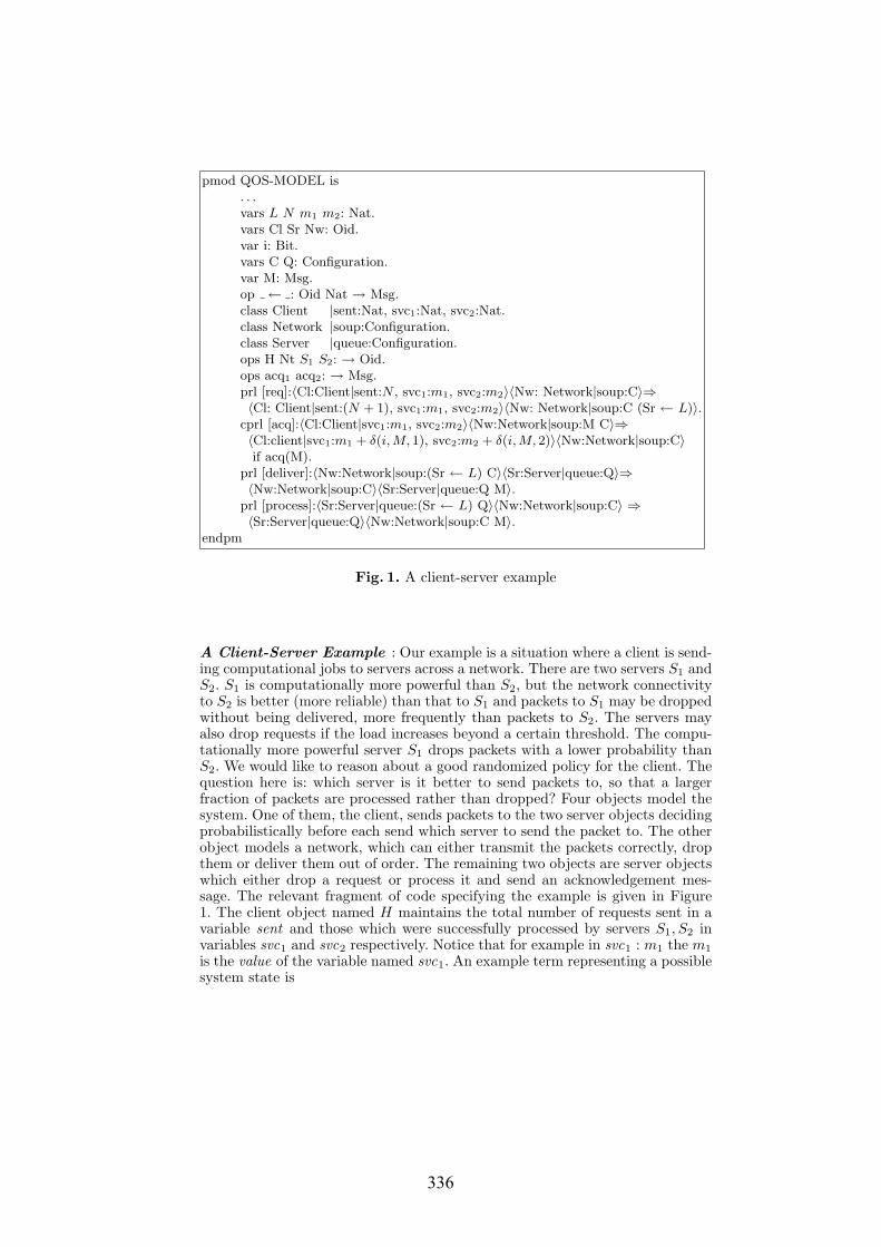
pmod QOS-MODEL is. . .vars L N m1 m2: Nat.vars Cl Sr Nw: Oid.var i: Bit.vars C Q: Configuration.var M: Msg.op ← : Oid Nat → Msg.class Client |sent:Nat, svc1:Nat, svc2:Nat.class Network |soup:Configuration.class Server |queue:Configuration.ops H Nt S1 S2: → Oid.ops acq1 acq2: → Msg.prl [req]:〈Cl:Client|sent:N , svc1:m1, svc2:m2〉〈Nw: Network|soup:C〉⇒〈Cl: Client|sent:(N + 1), svc1:m1, svc2:m2〉〈Nw: Network|soup:C (Sr ← L)〉.

cprl [acq]:〈Cl:Client|svc1:m1, svc2:m2〉〈Nw:Network|soup:M C〉⇒〈Cl:client|svc1:m1 + δ(i, M, 1), svc2:m2 + δ(i, M, 2)〉〈Nw:Network|soup:C〉if acq(M).

prl [deliver]:〈Nw:Network|soup:(Sr ← L) C〉〈Sr:Server|queue:Q〉⇒〈Nw:Network|soup:C〉〈Sr:Server|queue:Q M〉.

prl [process]:〈Sr:Server|queue:(Sr ← L) Q〉〈Nw:Network|soup:C〉 ⇒〈Sr:Server|queue:Q〉〈Nw:Network|soup:C M〉.

endpm

Fig. 1. A client-server example

A Client-Server Example : Our example is a situation where a client is send-ing computational jobs to servers across a network. There are two servers S1 andS2. S1 is computationally more powerful than S2, but the network connectivityto S2 is better (more reliable) than that to S1 and packets to S1 may be droppedwithout being delivered, more frequently than packets to S2. The servers mayalso drop requests if the load increases beyond a certain threshold. The compu-tationally more powerful server S1 drops packets with a lower probability thanS2. We would like to reason about a good randomized policy for the client. Thequestion here is: which server is it better to send packets to, so that a largerfraction of packets are processed rather than dropped? Four objects model thesystem. One of them, the client, sends packets to the two server objects decidingprobabilistically before each send which server to send the packet to. The otherobject models a network, which can either transmit the packets correctly, dropthem or deliver them out of order. The remaining two objects are server objectswhich either drop a request or process it and send an acknowledgement mes-sage. The relevant fragment of code specifying the example is given in Figure1. The client object named H maintains the total number of requests sent in avariable sent and those which were successfully processed by servers S1, S2 invariables svc1 and svc2 respectively. Notice that for example in svc1 : m1 the m1

is the value of the variable named svc1. An example term representing a possiblesystem state is

336

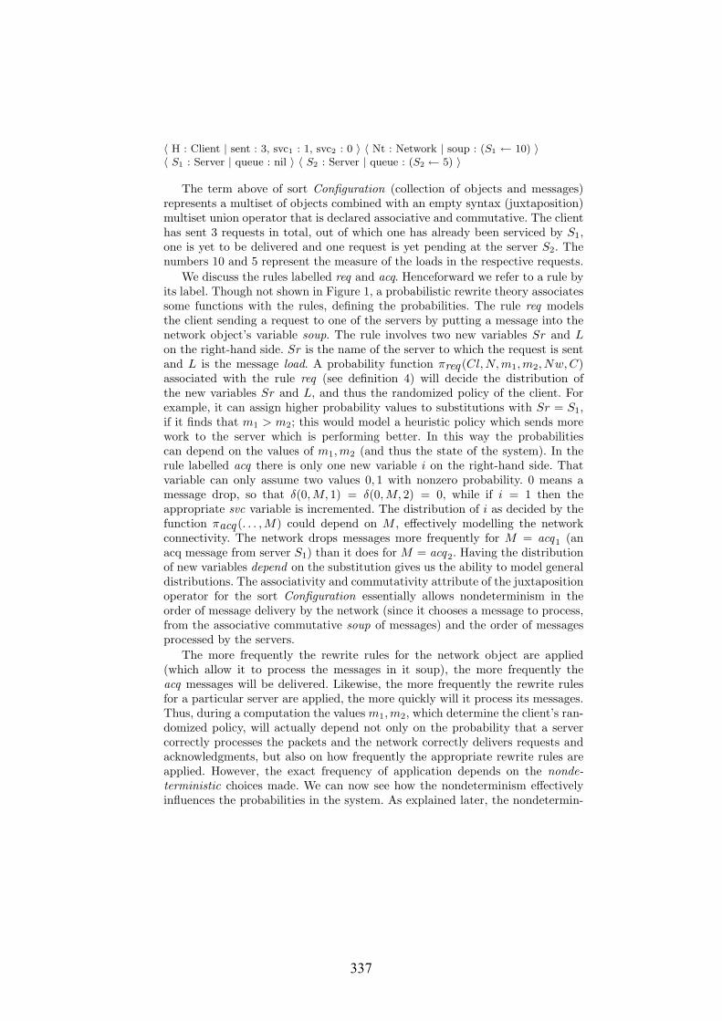
〈 H : Client | sent : 3, svc1 : 1, svc2 : 0 〉 〈 Nt : Network | soup : (S1 ← 10) 〉〈 S1 : Server | queue : nil 〉 〈 S2 : Server | queue : (S2 ← 5) 〉

The term above of sort Configuration (collection of objects and messages)represents a multiset of objects combined with an empty syntax (juxtaposition)multiset union operator that is declared associative and commutative. The clienthas sent 3 requests in total, out of which one has already been serviced by S1,one is yet to be delivered and one request is yet pending at the server S2. Thenumbers 10 and 5 represent the measure of the loads in the respective requests.

We discuss the rules labelled req and acq. Henceforward we refer to a rule byits label. Though not shown in Figure 1, a probabilistic rewrite theory associatessome functions with the rules, defining the probabilities. The rule req modelsthe client sending a request to one of the servers by putting a message into thenetwork object’s variable soup. The rule involves two new variables Sr and Lon the right-hand side. Sr is the name of the server to which the request is sentand L is the message load. A probability function πreq (Cl, N, m1, m2, Nw, C)associated with the rule req (see definition 4) will decide the distribution ofthe new variables Sr and L, and thus the randomized policy of the client. Forexample, it can assign higher probability values to substitutions with Sr = S1,if it finds that m1 > m2; this would model a heuristic policy which sends morework to the server which is performing better. In this way the probabilitiescan depend on the values of m1,m2 (and thus the state of the system). In therule labelled acq there is only one new variable i on the right-hand side. Thatvariable can only assume two values 0, 1 with nonzero probability. 0 means amessage drop, so that δ(0,M, 1) = δ(0,M, 2) = 0, while if i = 1 then theappropriate svc variable is incremented. The distribution of i as decided by thefunction πacq (. . . , M) could depend on M , effectively modelling the networkconnectivity. The network drops messages more frequently for M = acq1 (anacq message from server S1) than it does for M = acq2. Having the distributionof new variables depend on the substitution gives us the ability to model generaldistributions. The associativity and commutativity attribute of the juxtapositionoperator for the sort Configuration essentially allows nondeterminism in theorder of message delivery by the network (since it chooses a message to process,from the associative commutative soup of messages) and the order of messagesprocessed by the servers.

The more frequently the rewrite rules for the network object are applied(which allow it to process the messages in it soup), the more frequently theacq messages will be delivered. Likewise, the more frequently the rewrite rulesfor a particular server are applied, the more quickly will it process its messages.Thus, during a computation the values m1,m2, which determine the client’s ran-domized policy, will actually depend not only on the probability that a servercorrectly processes the packets and the network correctly delivers requests andacknowledgments, but also on how frequently the appropriate rewrite rules areapplied. However, the exact frequency of application depends on the nonde-terministic choices made. We can now see how the nondeterminism effectivelyinfluences the probabilities in the system. As explained later, the nondetermin-

337

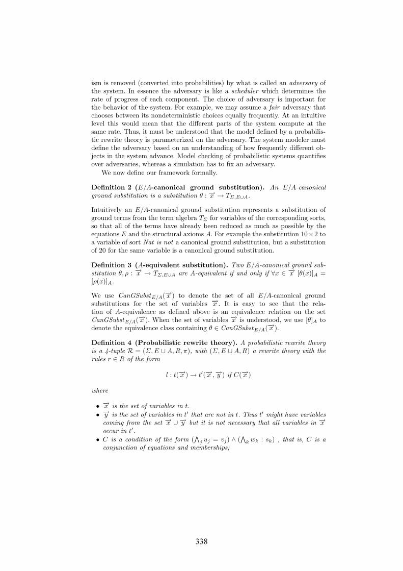
ism is removed (converted into probabilities) by what is called an adversary ofthe system. In essence the adversary is like a scheduler which determines therate of progress of each component. The choice of adversary is important forthe behavior of the system. For example, we may assume a fair adversary thatchooses between its nondeterministic choices equally frequently. At an intuitivelevel this would mean that the different parts of the system compute at thesame rate. Thus, it must be understood that the model defined by a probabilis-tic rewrite theory is parameterized on the adversary. The system modeler mustdefine the adversary based on an understanding of how frequently different ob-jects in the system advance. Model checking of probabilistic systems quantifiesover adversaries, whereas a simulation has to fix an adversary.

We now define our framework formally.

Definition 2 (E/A-canonical ground substitution). An E/A-canonicalground substitution is a substitution θ : −→x → TΣ,E∪A.

Intuitively an E/A-canonical ground substitution represents a substitution ofground terms from the term algebra TΣ for variables of the corresponding sorts,so that all of the terms have already been reduced as much as possible by theequations E and the structural axioms A. For example the substitution 10×2 toa variable of sort Nat is not a canonical ground substitution, but a substitutionof 20 for the same variable is a canonical ground substitution.

Definition 3 (A-equivalent substitution). Two E/A-canonical ground sub-stitution θ, ρ : −→x → TΣ,E∪A are A-equivalent if and only if ∀x ∈ −→x [θ(x)]A =[ρ(x)]A.

We use CanGSubstE/A(−→x ) to denote the set of all E/A-canonical groundsubstitutions for the set of variables −→x . It is easy to see that the rela-tion of A-equivalence as defined above is an equivalence relation on the setCanGSubstE/A(−→x ). When the set of variables −→x is understood, we use [θ]A todenote the equivalence class containing θ ∈ CanGSubstE/A(−→x ).

Definition 4 (Probabilistic rewrite theory). A probabilistic rewrite theoryis a 4-tuple R = (Σ, E ∪ A,R, π), with (Σ, E ∪ A,R) a rewrite theory with therules r ∈ R of the form

l : t(−→x ) → t′(−→x ,−→y ) if C(−→x )

where

• −→x is the set of variables in t.• −→y is the set of variables in t′ that are not in t. Thus t′ might have variables

coming from the set −→x ∪ −→y but it is not necessary that all variables in −→xoccur in t′.

• C is a condition of the form (∧

j uj = vj) ∧ (∧

k wk : sk) , that is, C is aconjunction of equations and memberships;

338

and π is a function assigning to each rewrite rule r ∈ R a function

πr : [[C]] → PFun(CanGSubstE/A(−→y ),Fr)

where [[C]] = [µ]A ∈ CanGSubstE/A(−→x ) | E ∪ A ` µ(C) is the set of E/A-canonical substitutions for −→x satisfying the condition C, and Fr is a σ-algebraon CanGSubstE/A(−→y ). We denote a rule r together with its associated functionπr, by the notation

l : t(−→x ) → t′(−→x ,−→y ) if C(−→x ) with probability πr(−→x )

We denote the class of probabilistic rewrite theories by PRwTh . Notice thefollowing points in the definition

1. Rewrite rules may have new variables −→y on the right-hand side.2. The condition C(−→x ) on the right-hand side depends only on the variables−→x occurring in the term t(−→x ) on the left-hand side.3. The condition C(−→x ) is simply a conjunction of equations and memberships

(but no rewrites).4. πr(−→x ) specifies, for each substitution θ for the variables −→x , the probability

of choosing a substitution ρ for the −→y . In the next section we explain howthis is done.

3.1 Semantics of Probabilistic Rewrite Theories

Let R = (Σ,E ∪A,R, π) be a probabilistic rewrite theory such that:

1. E is confluent, terminating and sort-decreasing modulo A [2].2. the rules R are coherent with E modulo A [4].

We also assume a choice for each rule r of an Fr-cover αr : CanGSubstE/A(−→y ) →Fr. This Fr-cover will be used to assign probabilities to rewrite steps. Its choicewill depend on the particular problem under consideration.

Definition 5 (Context). A context C is a Σ-term with a single occurrence ofa single variable, ¯, called the hole. Two contexts C and C′ are A-equivalent ifand only if A ` (∀¯) C = C′.Notice that the relation of A-equivalence for contexts as defined above, is anequivalence relation on the set of contexts. We use [C]A for the equivalence classcontaining context C. For example the term

¯ 〈 Nt : Network | soup : (S1 ← 10) 〉〈 S1 : Server | queue : nil 〉 〈 S2 : Server | queue : (S2 ← 5) 〉

is a context.

Definition 6 (R/A-matches). Given [u]A ∈ CanΣ,E/A, its R/A-matches aretriples ([C]A, r, [θ]A), where if r ∈ R is a rule

l : t(−→x ) → t′(−→x ,−→y ) if C(−→x ) with probability πr(−→x )

then [θ]A ∈ [[C]], that is [θ]A satisfies condition C and [u]A = [C(¯ ← θ(t))]A,so [u]A is the same as θ applied to the term t(−→x ) and placed in the context.

339

Consider the canonical-term

〈 H : Client | sent : 3, svc1 : 1, svc2 : 0 〉 〈 Nt : Network | soup : (S1 ← 10) 〉〈 S1 : Server | queue : nil 〉 〈 S2 : Server | queue : (S2 ← 5) 〉

Looking at the code in Figure 1, one of the R/A-matches for the equivalenceclass of the above term is the triple ([C]A, req, [θ]A) such that

C = ¯ 〈 Nt : Network | soup : (S1 ← 10) 〉〈 S1 : Server | queue : nil 〉 〈 S2 : Server | queue : (S2 ← 5) 〉

and θ is such that

θ(Cl) = H, θ(N) = 3, θ(m1) = 1, θ(m2) = 0.

Definition 7 (E/A-canonical one-step R-rewrite). An E/A-canonical one-step R-rewrite is a labelled transition of the form,

[u]A([C]A,r,[θ]A,[ρ]A)−−−−−−−−−−−→ [v]A

where

1. [u]A, [v]A ∈ CanΣ,E/A

2. ([C]A, r, [θ]A) is an R/A-match of [u]A3. [ρ]A ∈ CanGSubstE/A(−→y )4. [v]A = [C(¯ ← t′(θ(−→x ), ρ(−→y )))]A, where θ, ρ|−→x = θ and θ, ρ|−→y = ρ.

We associate the probability πr(αr(ρ)) with this transition. We can now see whythe Fr cover αr was needed. The nondeterminism associated with the choice ofthe R/A-match must be removed in order to associate a probability space overthe space of computations (which are infinite sequences of canonical one step R-rewrites). The nondeterminism is removed by what is called an adversary of thesystem, which defines a probability distribution over the set of R/A-matches. In[9] a probability space is associated over the set of computation paths. To do this,an adversary for the system is fixed. We have also shown in [9] that probabilisticrewrite theories have great expressive power. They can express various knownmodels of probabilistic systems like Continuous Time Markov Chains [8], MarkovDecision Processes [10] and even Generalized Semi Markov Processes [7]. Wealso propose a temporal logic, to express properties of interest in probabilisticsystems. The details can be found in [9].

Probabilistic rewrite theories can be used to model probabilistic actor sys-tems [1]. Actors, which are inherently asynchronous, can be modelled natu-rally using object based rewriting. In probabilistic actor systems we may beinterested in modelling message delay distributions among other probabilis-tic entities. However because time acts as a global synchronization parame-ter the natural encoding using objects, computing by their own rewrite rulesis insufficient. The technique of delayed messages helps us to correctly encode

340

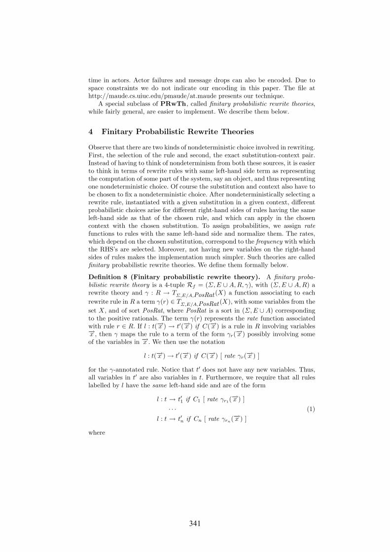
time in actors. Actor failures and message drops can also be encoded. Due tospace constraints we do not indicate our encoding in this paper. The file athttp://maude.cs.uiuc.edu/pmaude/at.maude presents our technique.

A special subclass of PRwTh, called finitary probabilistic rewrite theories,while fairly general, are easier to implement. We describe them below.

4 Finitary Probabilistic Rewrite Theories

Observe that there are two kinds of nondeterministic choice involved in rewriting.First, the selection of the rule and second, the exact substitution-context pair.Instead of having to think of nondeterminism from both these sources, it is easierto think in terms of rewrite rules with same left-hand side term as representingthe computation of some part of the system, say an object, and thus representingone nondeterministic choice. Of course the substitution and context also have tobe chosen to fix a nondeterministic choice. After nondeterministically selecting arewrite rule, instantiated with a given substitution in a given context, differentprobabilistic choices arise for different right-hand sides of rules having the sameleft-hand side as that of the chosen rule, and which can apply in the chosencontext with the chosen substitution. To assign probabilities, we assign ratefunctions to rules with the same left-hand side and normalize them. The rates,which depend on the chosen substitution, correspond to the frequency with whichthe RHS’s are selected. Moreover, not having new variables on the right-handsides of rules makes the implementation much simpler. Such theories are calledfinitary probabilistic rewrite theories. We define them formally below.

Definition 8 (Finitary probabilistic rewrite theory). A finitary proba-bilistic rewrite theory is a 4-tuple Rf = (Σ, E ∪ A,R, γ), with (Σ, E ∪ A, R) arewrite theory and γ : R → TΣ,E/A,PosRat (X) a function associating to eachrewrite rule in R a term γ(r) ∈ TΣ,E/A,PosRat (X), with some variables from theset X, and of sort PosRat, where PosRat is a sort in (Σ, E ∪ A) correspondingto the positive rationals. The term γ(r) represents the rate function associatedwith rule r ∈ R. If l : t(−→x ) → t′(−→x ) if C(−→x ) is a rule in R involving variables−→x , then γ maps the rule to a term of the form γr(−→x ) possibly involving someof the variables in −→x . We then use the notation

l : t(−→x ) → t′(−→x ) if C(−→x ) [ rate γr(−→x ) ]

for the γ-annotated rule. Notice that t′ does not have any new variables. Thus,all variables in t′ are also variables in t. Furthermore, we require that all ruleslabelled by l have the same left-hand side and are of the form

l : t → t′1 if C1 [ rate γr1(−→x ) ]

· · · (1)l : t → t′n if Cn [ rate γrn

(−→x ) ]

where

341

1. −→x = fvars(t) ⊇ ⋃1≤i≤n fvars(t′i) ∪ fvars(Ci), that is the terms t′i and the

conditions Ci do not have any variables other than −→x , the set of variablesin t.

2. Ci is of the form (∧

j uij = vij) ∧ (∧

k wik : sik) , that is, condition Ci is aconjunction of equations and memberships.1

We denote the class of finitary probabilistic rewrite theories by FPRTh.

4.1 Semantics of Finitary Probabilistic Rewrite Theories

Given a finitary probabilistic rewrite theory Rf = (Σ, E ∪ A, R, γ), we canexpress it as a probabilistic rewrite theoryR•f , by defining a map FR : Rf 7→ R•f ,with R•f = (Σ•, E• ∪A,R•, π•) and (Σ, E ∪A) ⊆ (Σ•, E• ∪A), in the followingway. We encode each group of rules in R with label l of the form 1 above by asingle probabilistic rewrite rule2

t(−→x ) → proj (i, (t′1(−→x ), . . . , t′n(−→x ))) if C1(−→x ) or . . . or Cn(−→x ) = true

with probability πr(−→x )

in R•. Corresponding to each such rule, we add to Σ• the sort [1 : n], with con-stants 1, . . . , n :→ [1 : n], and the projection operator proj : [1 : n] k . . . k → k.We also add to E• the equations proj (i, t1, . . . , tn) = ti for each i ∈ 1, . . . , n.Note that the only new variable on the righthand side is i, and thereforeCanGSubstE/A(i) ∼= 1, . . . , n. We consider the σ-algebra P(1, . . . , n) on1, . . . , n. Then πr is a function

πr : [[C]] → PFun(1, . . . , n,P(1, . . . , n))

defined as follows. If θ is such that C1(θ(−→x )) or . . . or Cn(θ(−→x )) = true, thenπθ = πr(θ) defined as

πθ(i) =?γri(θ(

−→x ))?γr1(θ(

−→x ))+?γr2(θ(−→x )) + · · ·+?γrn(θ(−→x ))

where, if Ci(θ(−→x )) = true, then ?γri(θ(−→x )) = γri

(θ(−→x )) and ?γri(θ(−→x )) = 0

otherwise. The semantics of Rf computations is now defined in terms of itsassociated theory R•f in the standard way, by choosing the singleton F-coverαr : 1, . . . , n → P(1, . . . , n) mapping each i to i.1 The requirement fvars(Ci) ⊆ fvars(t) can be relaxed by allowing new variables in

Ci to be introduced in “matching equations” in the sense of [4]. Then these newvariables can also appear in t′i.

2 By the assumption that (Σ, E ∪ A) is confluent, sort-decreasing, and terminatingmodulo A, and by a metatheorem of Bergstra and Tucker, any condition C of theform (

∧i ui = vi ∧

∧j wj : sj) can be replaced in an appropriate protecting en-

richment (Σ, E ∪ A) of (Σ, E ∪ A) by a semantically equivalent Boolean condition

C = true.

342

5 The PMaude Tool

We have developed an interpreter called PMaude , which provides a frame-work for specification and execution of finitary probabilistic rewrite theories.The PMaude interpreter has been built on top of Maude 2.0 [4,3] using theFull-Maude library [6]. We describe below how a finitary probabilistic rewritetheory is specified in our implemented framework and discuss some of the im-plementation details.

Consider a finitary probabilistic rewrite theory with k distinct rewrite labelsand with ni rewrite rules for the ith distinct label, for i = 1, 2, . . . , k.

l1 : t1 → t′11 if C11 [ rate γ11(−→x ) ]

· · ·l1 : t1 → t′1n1 if C1n1 [ rate γ1n1(

−→x ) ]

· · ·lk : tk → t′k1 if Ck1 [ rate γk1(

−→x ) ]

· · ·lk : tk → t′knk

if Cknk [ rate γknk (−→x ) ]

At one level we want all rewrite rules in the specification to have distinct la-bels, so that we have low level control over these rules, while at the conceptuallevel, groups of rules must have the same label. We achieve this by giving twolabels: one, common to a group and corresponding to the group’s label l at thebeginning, and another, unique for each rule, at the end. The above finitaryprobabilistic rewrite theory can be specified as follows in PMaude.

pmod FINITARY-EXAMPLE iscprl [l1] : t1 ⇒ t′11 if C11 [rate γ11(x1, . . . ) ] [metadata “l11 . . . ” ] .. . .cprl [l1] : t1 ⇒ t′1n1 if C1n1 [rate γ1n1(x1, . . . ) ] [metadata “l1n1 . . . ” ] .. . .cprl [lk] : tk ⇒ t′k1 if Ck1 [rate γk1(x1, . . . ) ] [metadata “lk1 . . . ” ] .. . .cprl [lk] : tk ⇒ t′knk

if Cknk [rate γknk (x1, . . . ) ] [metadata “lknk . . . ” ] .endpm

User input and output are supported as in Full Maude using the LOOP-MODEmodule. PMaude extends the Full Maude functions for parsing modules andany terms entered later by the user for rewriting purposes. Currently PMaudesupports four user commands. Two of these are low level commands used tochange seeds of pseudo-random generators. We shall not describe the imple-mentation of those two commands here. The other two commands are rewritecommands. Their syntax is as follows:

(prew t .)(prew -[n] t .)

The default module M in which these commands are interpreted is the last readprobabilistic module. The prew command is an instruction to the interpreter

343

to probabilistically rewrite the term t in the default module M , till no furtherrewrites are possible. Notice that this command may fail to terminate. Theprew -[n] command takes a natural number n specifying the maximum number ofprobabilistic rewrites to perform on the term t. This command always terminatesin at most n steps of rewriting. Both commands report the final term (if prewterminates).

The implementation of these commands is as follows. When the interpreteris given one of these commands, all possible one-step rewrites for t in the defaultmodule M are computed. Out of all possible groups l1, l2, .., lk in which somerewrite rule applies, one is chosen, uniformly at random. For the chosen groupli, all the rewrite rules li1, li2, .., lini associated with li, are guaranteed to havethe same left-hand side ti(x1, x2, ..). From all possible canonical substitution,context pairs ([θ]A, [C]A) for the variables xj , representing successful matches ofti(x1, x2, ..) with the given term t, that is, matches that also satisfy one of theconditions Cij , one of the matches is chosen uniformly at random. The two stepsabove also define the exact adversary we associate to a given finitary probabilisticrewrite theory in our implementation. If there are m groups, li1 , . . . , lim , in whichsome rule applies and vj matches in total for group lij then the adversary choosesa match in group lij with probability 1

mvj. To choose the exact rewrite rule lij

to apply, use of the rate functions is made. The values of the various ratesγip are calculated for those rules lip such that [θ]A satisfies the condition ofthe rule lip. Then these rates are normalized and the choice of the rule lij ismade probabilistically, based on the calculated rates. This rewrite rule is thenapplied to the term t, in the chosen context with the chosen substitution. If theinterpreter finds no successful matches for a given term, or if it has completedthe maximum number of rewrites specified, it immediately reports that termas the answer. Since rates can depend on the substitution, this allows users tospecify systems where probabilities are determined by the state.

PMaude can be used as a simulator for finitary probabilistic rewrite theories.The programmer must supply the system specification as a PMaude moduleand a start term to rewrite. To obtain different results the seeds for the randomnumber generators must be changed at each invocation. This can be done byusing a scripting language to call the interpreter repeatedly but with differentseeds before each execution.

We have specified the client-server example discussed in Section 3 inPMaude with the following parameters: The client only sends two kinds ofpackets, loads 5 and 10, with equal probability. The request messages for S1, S2

are dropped with probabilities 2/7 and 1/6 respectively, while acknowledgementmessages for S1, S2 are dropped with probabilities 1/6, 1/11 respectively. Wealso chose S1 to drop processing of a request with probability 1/7 as opposed to3/23 when its load was at least 100, while for S2 the load limit was 40 but theprobabilities of dropping requests were 1/7 and 3/19. We performed some simu-lations and, after a number of runs, we computed the ratio (svc1 + svc2)/sent asa measure of the quality of service for the client. Simulations showed that amongstatic policies, namely those where the client did not adapt sending probabilities

344

on the fly, that of sending twice as often to server S2 than to S1 was better thanmost others.

The complete code for the PMaude interpreter, as well as several otherexample files, can be found at http:/maude.cs.uiuc.edu/pmaude/pmaude.html.

6 Conclusions and Future Work

Probabilistic rewrite theories provide a general semantic framework supportinghigh level probabilistic specification of systems; in fact, we have shown how var-ious well known probabilistic models can be expressed in our framework [9].The present work shows how our framework applies to concurrent object basedsystems. For a fairly general subclass, namely finitary probabilistic rewrite the-ories, we have implemented a simulator PMaude and have exercised it on somesimple examples. We are currently carrying out more case studies. We have alsoidentified several aspects of the theory and the PMaude tool that need furtherdevelopment.

On the more theoretical side, we feel research is needed in three areas. First, itis important to develop a general model of probabilistic systems with concurrentprobabilistic actions, as opposed to the current interleaving semantics. Second,deductive and analytic methods for property verification of probabilistic systems,based on our current framework is an important open problem. Algorithms totranslate appropriate subclasses to appropriate representations enabling use ofexisting model checkers, should be developed and implemented.

Third, we think that allowing the probability function πr to depend not onlyon the substitution, but also on the context would give us more modelling power.Specifically, it would enable us to represent applications where the probabilitydistributions of certain variables, such as message delays, depend on functionsof the entire state of the system, for example, on the congestion in the network.Such situations can also be modelled in our current framework but at the expenseof using rewrite rules at the top-level, whose substitutions capture global systemparameters. Such rules can modify the entire system at once as opposed to justmodifying local fragments, but at the cost of violating the modularity principleof concurrent objects or actors.

On the implementation side, an extension of the PMaude framework toenable specification of more general classes of probabilistic rewrite theories andadversaries is highly desirable. This will allow the generation of simulation tracesfor the system under consideration and can be used as a tool to implement themodel independent Monte-Carlo simulation and acceptance sampling methodsfor probabilistic validation of properties [14]. As an application of our theory,we believe that it will be fruitful to model networked embedded systems, whereapart from time, there are other continuous state variables, such as battery poweror temperature, whose behavior may be stochastic. Moreover, the properties ofinterest are often a statistical aggregation of many observations.

345

7 Acknowledgement

The work is supported in part by the Defense Advanced Research ProjectsAgency (the DARPA IPTO TASK Program, contract number F30602-00-2-0586and the DARPA IXO NEST Program, contract number F33615-01-C-1907) andthe ONR Grant N00014-02-1-0715. We would like to thank Wooyoung Kim forreading a previous version of this paper and giving us valuable feedback andJoost-Pieter Katoen for very helpful discussions and pointers to references.

References

1. G. Agha, I. A. Mason, S. F. Smith, and C. L. Talcott. A foundation for actorcomputation. Journal of Functional Programming, 7(1):1–72, 1997.

2. A. Bouhoula, J.-P. Jouannaud, and J. Meseguer. Specification and proof in mem-bership equational logic. Theoretical Computer Science, 236(1–2):35–132, 2000.

3. M. Clavel, F. Duran, S. Eker, P. Lincoln, N. Martı-Oliet, J. Meseguer, and J. Que-sada. Towards maude 2.0. In K. Futatsugi, editor, Electronic Notes in TheoreticalComputer Science, volume 36. Elsevier, 2001.

4. M. Clavel, F. Duran, S. Eker, P. Lincoln, N. Martı-Oliet, J. Meseguer, and J. Que-sada. Maude: specification and programming in rewriting logic. Theoretical Com-puter Science, 285:187–243, 2002.

5. M. Clavel, F. Duran, S. Eker, P. Lincoln, N. Martı-Oliet, J. Meseguer, and C. Tal-cott. Maude 2.0 Manual, Version 1.0, june 2003. http://maude.cs.uiuc.edu/

manual/maude-manual.pdf.6. F. Duran and J. Meseguer. Parameterized theories and views in full maude 2.0. In

K. Futatsugi, editor, Electronic Notes in Theoretical Computer Science, volume 36.Elsevier, 2001.

7. P. Glynn. The role of generalized semi-Markov processes in simulation outputanalysis, 1983.

8. J.-P. Katoen, M. Kwiatkowska, G. Norman, and D. Parker. Faster and symbolicCTMC model checking. Lecture Notes in Computer Science, 2165, 2001.

9. N. Kumar, K. Sen, J. Meseguer, and G. Agha. Probabilistic rewrite theories: Unify-ing models, logics and tools. Technical Report UIUCDCS-R-2003-2347, Universityof Illinois at Urbana-Champaign, May 2003.

10. M. Z. Kwiatkowska, G. Norman, and D. Parker. Prism: Probabilistic symbolicmodel checker, 2002.

11. J. Meseguer. Conditional rewriting logic as a unified model of concurrency. Theo-retical Computer Science, 96:73–155, 1992.

12. J. Meseguer. A logical theory of concurrent objects and its realization in the Maudelanguage. In G. Agha, P. Wegner, and A. Yonezawa, editors, Research Directionsin Concurrent Object-Oriented Programming, pages 314–390. MIT Press, 1993.

13. J. Meseguer. Membership algebra as a logical framework for equational specifica-tion. In F. Parisi-Presicce, editor, Proc. WADT’97, pages 18–61. Springer LNCS1376, 1998.

14. H. L. S. Younes and R. G. Simmons. Probabilistic verification of discrete eventsystems using acceptance sampling. In E. Brinksma and K. G. Larsen, editors,Proceedings of the 14th International Conference on Computer Aided Verification,volume 2404 of Lecture Notes in Computer Science, pages 223–235, Copenhagen,Denmark, July 2002. Springer.

346

Electronic Notes in Theoretical Computer Science 71 (2003)URL: http://www.elsevier.nl/locate/entcs/volume71.html 21 pages

An Executable Specification of AsynchronousPi-Calculus Semantics and May Testing in

Maude 2.0

Prasanna Thati Koushik Sen

Department of Computer ScienceUniversity of Illinois at Urbana-Champaign

thati,ksen@cs.uiuc.edu

Narciso Martı-Oliet

Dpto. de Sistemas Informaticos y ProgramacionUniversidad Complutense de Madrid, Spain

narciso@sip.ucm.es

Abstract

We describe an executable specification of the operational semantics of an asyn-chronous version of the π-calculus in Maude by means of conditional rewrite ruleswith rewrites in the conditions. We also present an executable specification of themay testing equivalence on non-recursive asynchronous π-calculus processes, usingthe Maude metalevel. Specifically, we describe our use of the metaSearch opera-tion to both calculate the set of all finite traces of a non-recursive process, and tocompare the trace sets of two processes according to a preorder relation that char-acterizes may testing in asynchronous π-calculus. Thus, in both the specification ofthe operational semantics and the may testing, we make heavy use of new featuresintroduced in version 2.0 of the Maude language and system.

Key words: π-calculus, asynchrony, may testing, traces, Maude.

1 Introduction

Since its introduction in the seminal paper [11] by Milner, Parrow, and Walker,the π-calculus has become one of the most studied calculus for name-basedmobility of processes, where processes are able to exchange names over chan-nels so that the communication topology can change during the computation.The operational semantics of the π-calculus has been defined for several differ-ent versions of the calculus following two main styles. The first is the labelledtransition system style according to the SOS approach introduced by Plotkin

c©2003 Published by Elsevier Science B. V.

347

Thati, Sen, and Martı-Oliet

[13]. The second is the reduction style, where first an equivalence is imposedon syntactic processes (typically to make syntax more abstract with respectto properties of associativity and/or commutativity of some operators), andthen some reduction or rewrite rules express how the computation proceedsby communication between processes.

The first specification of the π-calculus operational semantics in rewritinglogic was developed by Viry in [19], in a reduction style making use of deBruijn indexes, explicit substitutions, and reduction strategies in Elan [6].This presentation was later improved by Stehr [14] by making use of a genericcalculus for explicit substitutions, known as CINNI, which combines the bestof the approaches based on standard variables and de Bruijn indices, and thathas been implemented in Maude.

Our work took the work described above as a starting point, togetherwith recent work by Verdejo and Martı-Oliet [18] showing how to use the newfeatures of Maude 2.0 in the implementation of a semantics in the labelledtransition system style for CCS. This work makes essential use of conditionalrewrite rules with rewrites in the conditions, so that an inference rule in thelabelled transition system of the form

P1 → Q1 . . . Pn → Qn

P0 → Q0

becomes a conditional rewrite rule of the form

P0 −→ Q0 if P1 −→ Q1 ∧ . . . ∧ Pn −→ Qn,

where the condition includes rewrites. These rules are executable in version 2.0of the Maude language and system [7]. However, this is not enough, becauseit is necessary to have some control on the application of rules. Typically,rewrite rules can be applied anywhere in a term, while the transitions in theoperational semantics for CCS or the π-calculus in the SOS style only takeplace at the top. The new frozen attribute available in Maude 2.0 makes thispossible, because the declaration of an operator as frozen forbids rewriting itsarguments, thus providing another way of controlling the rewriting process.Rewrite conditions when applying conditional rules are solved by means ofan implicit search process, which is also available to the user both at thecommand level and at the metalevel. The search command looks for all therewrites of a given term that match a given pattern satisfying some condition.Search is reified at the metalevel as an operation metaSearch.

In this way, our first contribution is a fully executable specification ofan operational semantics in the labelled transition system style for an asyn-chronous version of the π-calculus (the semantics for the synchronous case isobtained as a simple modification). This specification uses conditional rewriterules with rewrites in conditions and the CINNI calculus [14] for managingnames and bindings in the π-calculus. However, these two ingredients are notenough to obtain a fully executable specification. A central problem to over-come is that the transitions of a term can be infinitely branching. For instance,

2

348

Thati, Sen, and Martı-Oliet

the term x(y).P can evolve via an input action to one of an infinite family ofterms depending on the name received in the input at channel x. Our solutionis to define the transitions of a process relative to an execution environment.The environment is represented abstractly as a set of free (global) names thatthe environment may use while interacting with the process, and transitionsare modelled as rewrite rules over a pair consisting of a set of environmentnames together with a process.

Our next contribution is to implement the verification of the may-testingpreorder [12,3,5] between finitary (non-recursive) asynchronous π-calculus pro-cesses, using again ideas from [18] to calculate the set of all finite traces of aprocess. May testing is a specific instance of the notion of behavioral equiv-alence on π-calculus processes; in may testing, two processes are said to beequivalent if they have the same success properties in all experiments. Anexperiment consists of an observing process that runs in parallel and interactswith the process being tested, and success is defined as the observer signallinga special event. Viewing the occurrence of an event as something bad hap-pening, may testing can be used to reason about safety properties [4].

Since the definition of may testing involves a universal quantification overall observers, it is difficult to establish process equivalences directly from thedefinition. As a solution, alternate characterizations of the equivalence thatdo not resort to quantification over observers have been found. It is knownthat the trace semantics is an alternate characterization of may testing in(synchronous) π-calculus [3], while a variant of the trace semantics has beenshown to characterize may testing in an asynchronous setting [5]. Specifically,in both these cases, comparing two processes according to the may-testingpreorder amounts to comparing the set of all finite traces they exhibit. Wehave implemented for finite asynchronous processes, the comparison of tracesets proposed in [5]. We stress that our choice of specifying an asynchronousversion rather than the synchronous π-calculus, is because the characterizationof may testing for the asynchronous case is more interesting and difficult. Thesynchronous version can be specified in an executable way using similar butsimpler techniques.

Our first step in obtaining an executable specification of may testing isto obtain the set of all finite traces of a given process. This is done at theMaude metalevel by using the metaSearch operation to collect all results ofrewriting a given term. The second step is to specify a preorder relationbetween traces that characterizes may testing. We have represented the tracepreorder relation as a rewriting relation, i.e. the rules of inference that definethe trace preorder are again modeled as conditional rewrite rules. The finalstep is to check if two processes are related by the may preorder, i.e. whethera statement of the form P v Q is true or not. This step involves computingthe closure of a trace under the trace-preorder relation, again by means of themetaSearch operation. Thus, our work demonstrates the utility of the newmetalevel facilities available in Maude 2.0.

3

349

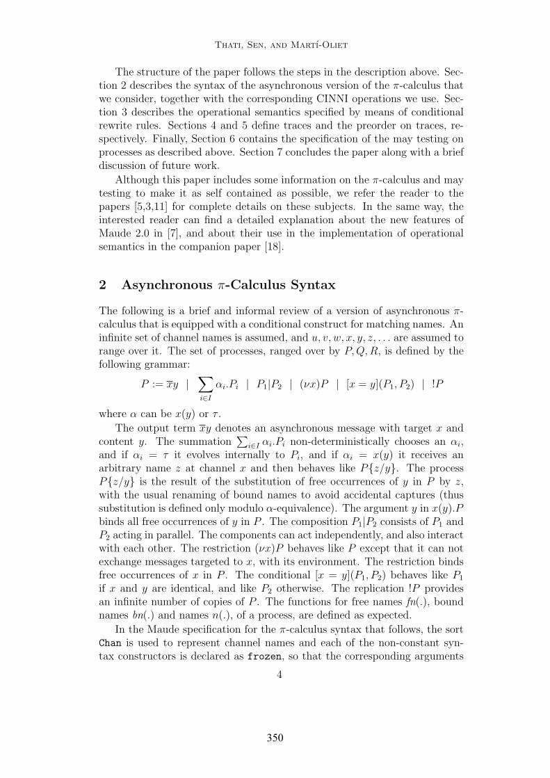
Thati, Sen, and Martı-Oliet

The structure of the paper follows the steps in the description above. Sec-tion 2 describes the syntax of the asynchronous version of the π-calculus thatwe consider, together with the corresponding CINNI operations we use. Sec-tion 3 describes the operational semantics specified by means of conditionalrewrite rules. Sections 4 and 5 define traces and the preorder on traces, re-spectively. Finally, Section 6 contains the specification of the may testing onprocesses as described above. Section 7 concludes the paper along with a briefdiscussion of future work.

Although this paper includes some information on the π-calculus and maytesting to make it as self contained as possible, we refer the reader to thepapers [5,3,11] for complete details on these subjects. In the same way, theinterested reader can find a detailed explanation about the new features ofMaude 2.0 in [7], and about their use in the implementation of operationalsemantics in the companion paper [18].

2 Asynchronous π-Calculus Syntax

The following is a brief and informal review of a version of asynchronous π-calculus that is equipped with a conditional construct for matching names. Aninfinite set of channel names is assumed, and u, v, w, x, y, z, . . . are assumed torange over it. The set of processes, ranged over by P, Q,R, is defined by thefollowing grammar:

P := xy |∑i∈I

αi.Pi | P1|P2 | (νx)P | [x = y](P1, P2) | !P

where α can be x(y) or τ .

The output term xy denotes an asynchronous message with target x andcontent y. The summation

∑i∈I αi.Pi non-deterministically chooses an αi,

and if αi = τ it evolves internally to Pi, and if αi = x(y) it receives anarbitrary name z at channel x and then behaves like Pz/y. The processPz/y is the result of the substitution of free occurrences of y in P by z,with the usual renaming of bound names to avoid accidental captures (thussubstitution is defined only modulo α-equivalence). The argument y in x(y).Pbinds all free occurrences of y in P . The composition P1|P2 consists of P1 andP2 acting in parallel. The components can act independently, and also interactwith each other. The restriction (νx)P behaves like P except that it can notexchange messages targeted to x, with its environment. The restriction bindsfree occurrences of x in P . The conditional [x = y](P1, P2) behaves like P1

if x and y are identical, and like P2 otherwise. The replication !P providesan infinite number of copies of P . The functions for free names fn(.), boundnames bn(.) and names n(.), of a process, are defined as expected.

In the Maude specification for the π-calculus syntax that follows, the sortChan is used to represent channel names and each of the non-constant syn-tax constructors is declared as frozen, so that the corresponding arguments

4

350

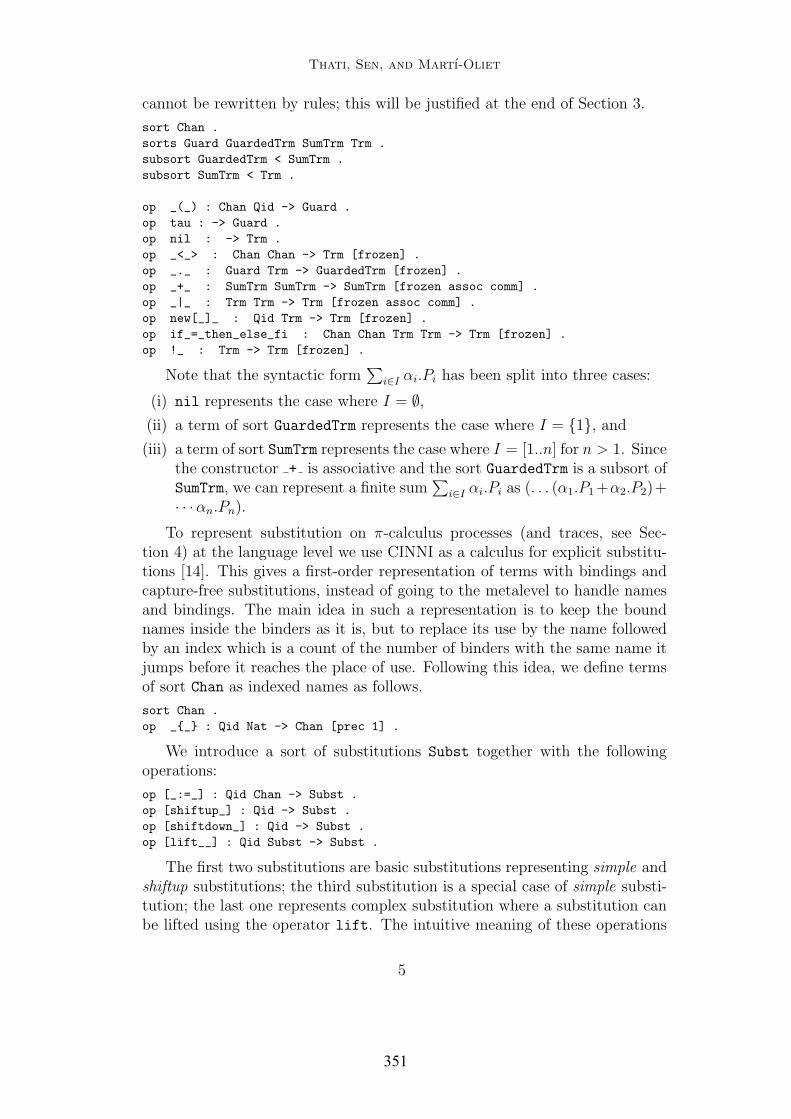
Thati, Sen, and Martı-Oliet

cannot be rewritten by rules; this will be justified at the end of Section 3.

sort Chan .sorts Guard GuardedTrm SumTrm Trm .subsort GuardedTrm < SumTrm .subsort SumTrm < Trm .

op _(_) : Chan Qid -> Guard .op tau : -> Guard .op nil : -> Trm .op _<_> : Chan Chan -> Trm [frozen] .op _._ : Guard Trm -> GuardedTrm [frozen] .op _+_ : SumTrm SumTrm -> SumTrm [frozen assoc comm] .op _|_ : Trm Trm -> Trm [frozen assoc comm] .op new[_]_ : Qid Trm -> Trm [frozen] .op if_=_then_else_fi : Chan Chan Trm Trm -> Trm [frozen] .op !_ : Trm -> Trm [frozen] .

Note that the syntactic form∑

i∈I αi.Pi has been split into three cases:

(i) nil represents the case where I = ∅,(ii) a term of sort GuardedTrm represents the case where I = 1, and

(iii) a term of sort SumTrm represents the case where I = [1..n] for n > 1. Sincethe constructor + is associative and the sort GuardedTrm is a subsort ofSumTrm, we can represent a finite sum

∑i∈I αi.Pi as (. . . (α1.P1 +α2.P2)+

· · ·αn.Pn).

To represent substitution on π-calculus processes (and traces, see Sec-tion 4) at the language level we use CINNI as a calculus for explicit substitu-tions [14]. This gives a first-order representation of terms with bindings andcapture-free substitutions, instead of going to the metalevel to handle namesand bindings. The main idea in such a representation is to keep the boundnames inside the binders as it is, but to replace its use by the name followedby an index which is a count of the number of binders with the same name itjumps before it reaches the place of use. Following this idea, we define termsof sort Chan as indexed names as follows.

sort Chan .op __ : Qid Nat -> Chan [prec 1] .

We introduce a sort of substitutions Subst together with the followingoperations:

op [_:=_] : Qid Chan -> Subst .op [shiftup_] : Qid -> Subst .op [shiftdown_] : Qid -> Subst .op [lift__] : Qid Subst -> Subst .

The first two substitutions are basic substitutions representing simple andshiftup substitutions; the third substitution is a special case of simple substi-tution; the last one represents complex substitution where a substitution canbe lifted using the operator lift. The intuitive meaning of these operations

5

351

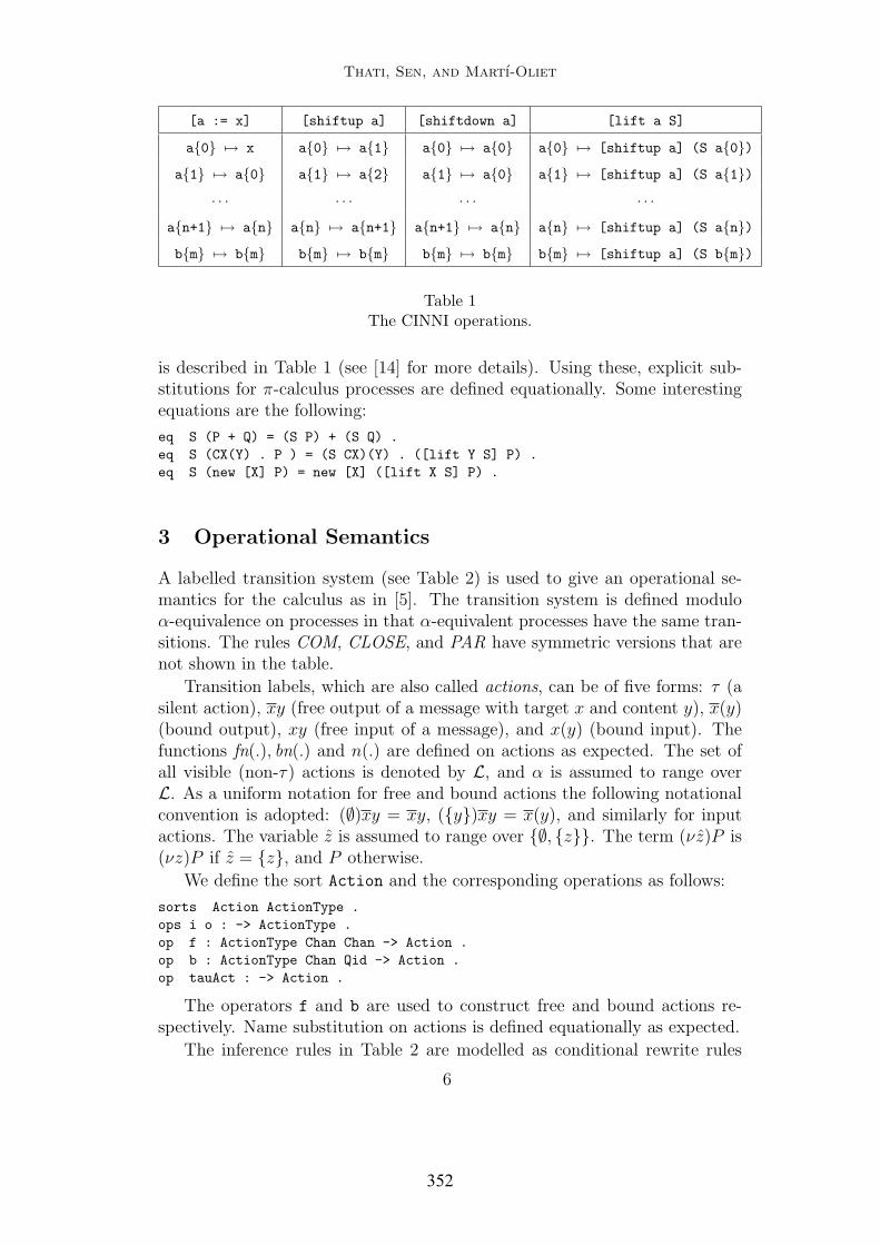
Thati, Sen, and Martı-Oliet

[a := x] [shiftup a] [shiftdown a] [lift a S]

a0 7→ x a0 7→ a1 a0 7→ a0 a0 7→ [shiftup a] (S a0)a1 7→ a0 a1 7→ a2 a1 7→ a0 a1 7→ [shiftup a] (S a1)

· · · · · · · · · · · ·an+1 7→ an an 7→ an+1 an+1 7→ an an 7→ [shiftup a] (S an)bm 7→ bm bm 7→ bm bm 7→ bm bm 7→ [shiftup a] (S bm)

Table 1The CINNI operations.

is described in Table 1 (see [14] for more details). Using these, explicit sub-stitutions for π-calculus processes are defined equationally. Some interestingequations are the following:

eq S (P + Q) = (S P) + (S Q) .eq S (CX(Y) . P ) = (S CX)(Y) . ([lift Y S] P) .eq S (new [X] P) = new [X] ([lift X S] P) .

3 Operational Semantics

A labelled transition system (see Table 2) is used to give an operational se-mantics for the calculus as in [5]. The transition system is defined moduloα-equivalence on processes in that α-equivalent processes have the same tran-sitions. The rules COM, CLOSE, and PAR have symmetric versions that arenot shown in the table.

Transition labels, which are also called actions, can be of five forms: τ (asilent action), xy (free output of a message with target x and content y), x(y)(bound output), xy (free input of a message), and x(y) (bound input). Thefunctions fn(.), bn(.) and n(.) are defined on actions as expected. The set ofall visible (non-τ) actions is denoted by L, and α is assumed to range overL. As a uniform notation for free and bound actions the following notationalconvention is adopted: (∅)xy = xy, (y)xy = x(y), and similarly for inputactions. The variable z is assumed to range over ∅, z. The term (νz)P is(νz)P if z = z, and P otherwise.

We define the sort Action and the corresponding operations as follows:

sorts Action ActionType .ops i o : -> ActionType .op f : ActionType Chan Chan -> Action .op b : ActionType Chan Qid -> Action .op tauAct : -> Action .

The operators f and b are used to construct free and bound actions re-spectively. Name substitution on actions is defined equationally as expected.

The inference rules in Table 2 are modelled as conditional rewrite rules

6

352

Thati, Sen, and Martı-Oliet

INP:∑

i∈I αi.Pixjz−→ Pjz/y j ∈ I, αj = xj(y)

TAU:∑

i∈I αi.Piτ−→ Pj j ∈ I, αj = τ

OUT: xyxy−→ 0

BINP:P

xy−→ P ′

Px(y)−→ P ′

y /∈ fn(P )

PAR:P1

α−→ P ′1

P1|P2α−→ P ′

1|P2

bn(α) ∩ fn(P2) = ∅ COM:P1

xy−→ P ′1 P2

xy−→ P ′2

P1|P2τ−→ P ′

1|P ′2

RES:P

α−→ P ′

(νy)Pα−→ (νy)P ′

y /∈ n(α) OPEN:P

xy−→ P ′

(νy)Px(y)−→ P ′

x 6= y

CLOSE:P1

x(y)−→ P ′1 P2

xy−→ P ′2

P1|P2τ−→ (νy)(P ′

1|P ′2)

y /∈ fn(P2) REP:P |!P α−→ P ′

!Pα−→ P ′

IF:P

α−→ P ′

[x = x](P, Q)α−→ P ′

ELSE:Q

α−→ Q′

[x = y](P, Q)α−→ Q′

x 6= y

Table 2A labelled transition system for asynchronous π-calculus.

with the premises as conditions of the rule. 1 Since rewrites do not have labelsunlike the labelled transitions, we make the label a part of the resulting term;thus rewrites corresponding to transitions in the operational semantics are ofthe form P ⇒ αQ.

Because of the INP and OPEN rules, the transitions of a term can beinfinitely branching. Specifically, in case of the INP rule there is one branchfor every possible name that can be received in the input. In case of the OPENrule, there is one branch for every name that is chosen to denote the privatechannel that is being emitted (note that the transition rules are defined onlymodulo α-equivalence). To overcome this problem, we define transitions overpairs of the form [CS] P, where CS is a set of channel names containing all thenames that the environment with which the process interacts, knows about.The set CS expands during bound input and output interactions when privatenames are exchanged between the process and its environment.

The infinite branching due to the INP rule is avoided by allowing only thenames in the environment set CS to be received in free inputs. Since CS isassumed to contain all the free names in the environment, an input argumentthat is not in CS would be a private name of the environment. Now, sincethe identifier chosen to denote the fresh name is irrelevant, all bound input

1 The symmetric versions missing in the table need not be implemented because the processconstructors + and | have been declared as commutative.

7

353

Thati, Sen, and Martı-Oliet

transitions can be identified to a single input. With these simplifications,the number of input transitions of a term become finite. Similarly, in theOPEN rule, since the identifier chosen to denote the private name emitted isirrelevant, instances of the rule that differ only in the chosen name are notdistinguished.

We discuss in detail the implementation of only a few of the inference rules;the reader is referred to the appendix for a complete list of all the rewrite rulesfor Table 2.

sorts EnvTrm TraceTrm .subsort EnvTrm < TraceTrm .op [_]_ : Chanset Trm -> EnvTrm [frozen] .op __ : Action TraceTrm -> TraceTrm [frozen] .

Note that the two operators are also declared above with the frozen at-tribute, forbidding in this way rewriting of their arguments, as justified at theend of this section.

The following non-conditional rule is for free inputs.

rl [Inp] : [CY CS] ((CX(X) . P) + SUM) =>f(i,CX,CY) ([CY CS] ([X := CY] P)) .

The next rule we consider is the one for bound inputs. Since the identifierchosen to denote the bound argument is irrelevant, we use the constant ’U

for all bound inputs, and thus ’U0 denotes the fresh channel received. Notethat in contrast to the BINP rule of Table 2, we do not check if ’U0 is in thefree names of the process performing the input, and instead we shift up thechannel indices appropriately, in both the set of environment names CS andthe process P in the righthand side and condition of the rule. This is justifiedbecause the transition target is within the scope of the bound name in theinput action. Note also that the channel CX in the action is not shifted downbecause it is out of the scope of the bound argument. The set of environmentnames is expanded by adding the received channel ’U0 to it. Finally, weuse a special constant flag of sort Chan, to ensure termination. We add aninstance of flag to the environment set of the rewrite in condition, so thatthe BINP rule is not fired again while evaluating the condition. Without thischeck, we will have a non-terminating execution in which the BINP rule isrepeatedly fired.

crl [BInp] : [CS] P => b(i,CX,’U) [’U0 [shiftup ’U] CS] P1if (not flag in CS) /\

CS1 := flag ’U0 [shiftup ’U] CS /\[CS1] [shiftup ’U] P => f(i,CX,’U0) [CS1] P1 .

The following rule treats the case of bound outputs.

crl [Open] : [CS] (new [X] P) => [shiftdown X] b(o,CY,X) [X0 CS1] P1if CS1 := [shiftup X] CS /\

[CS1] P => f(o,CY,X0) [CS1] P1 /\ X0 =/= CY .

Like in the case of bound inputs, we identify all bound outputs to a single

8

354

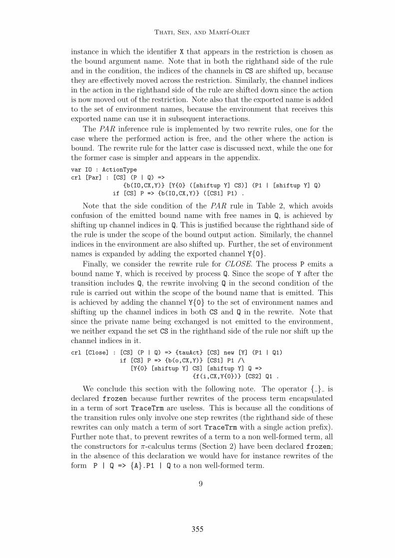
Thati, Sen, and Martı-Oliet

instance in which the identifier X that appears in the restriction is chosen asthe bound argument name. Note that in both the righthand side of the ruleand in the condition, the indices of the channels in CS are shifted up, becausethey are effectively moved across the restriction. Similarly, the channel indicesin the action in the righthand side of the rule are shifted down since the actionis now moved out of the restriction. Note also that the exported name is addedto the set of environment names, because the environment that receives thisexported name can use it in subsequent interactions.

The PAR inference rule is implemented by two rewrite rules, one for thecase where the performed action is free, and the other where the action isbound. The rewrite rule for the latter case is discussed next, while the one forthe former case is simpler and appears in the appendix.

var IO : ActionTypecrl [Par] : [CS] (P | Q) =>

b(IO,CX,Y) [Y0 ([shiftup Y] CS)] (P1 | [shiftup Y] Q)if [CS] P => b(IO,CX,Y) ([CS1] P1) .

Note that the side condition of the PAR rule in Table 2, which avoidsconfusion of the emitted bound name with free names in Q, is achieved byshifting up channel indices in Q. This is justified because the righthand side ofthe rule is under the scope of the bound output action. Similarly, the channelindices in the environment are also shifted up. Further, the set of environmentnames is expanded by adding the exported channel Y0.

Finally, we consider the rewrite rule for CLOSE. The process P emits abound name Y, which is received by process Q. Since the scope of Y after thetransition includes Q, the rewrite involving Q in the second condition of therule is carried out within the scope of the bound name that is emitted. Thisis achieved by adding the channel Y0 to the set of environment names andshifting up the channel indices in both CS and Q in the rewrite. Note thatsince the private name being exchanged is not emitted to the environment,we neither expand the set CS in the righthand side of the rule nor shift up thechannel indices in it.

crl [Close] : [CS] (P | Q) => tauAct [CS] new [Y] (P1 | Q1)if [CS] P => b(o,CX,Y) [CS1] P1 /\

[Y0 [shiftup Y] CS] [shiftup Y] Q =>f(i,CX,Y0) [CS2] Q1 .

We conclude this section with the following note. The operator isdeclared frozen because further rewrites of the process term encapsulatedin a term of sort TraceTrm are useless. This is because all the conditions ofthe transition rules only involve one step rewrites (the righthand side of theserewrites can only match a term of sort TraceTrm with a single action prefix).Further note that, to prevent rewrites of a term to a non well-formed term, allthe constructors for π-calculus terms (Section 2) have been declared frozen;in the absence of this declaration we would have for instance rewrites of theform P | Q => A.P1 | Q to a non well-formed term.

9

355

Thati, Sen, and Martı-Oliet

4 Trace Semantics

The set L∗ is the set of traces. The functions fn(.), bn(.) and n(.) are extendedto L∗ in the obvious way. The relation of α-equivalence on traces is definedas expected, and α-equivalent traces are not distinguished. The relation =⇒denotes the reflexive transitive closure of

τ−→, andβ

=⇒ denotes =⇒ β−→=⇒.

For s = l.s′, we inductively define Ps

=⇒ P ′ as Pl

=⇒ s′=⇒ P ′. We use P

s=⇒

as an abbreviation for Ps

=⇒ P ′ for some P ′. The set of traces that a processexhibits is then [|P |] = s | P

s=⇒.

In the implementation, we introduce a sort Trace as supersort of Actionto specify traces.

subsort Action < Trace .op epsilon : -> Trace .op _._ : Trace Trace -> Trace [assoc id: epsilon] .op [_] : Trace -> TTrace .

We define the operator [ ] to represent a complete trace. The motivationfor doing so is to restrict the equations and rewrite rules defined over traces tooperate only on a complete trace instead of a part of it. The following equationdefines α-equivalence on traces. Note that in a trace TR1.b(IO,CX,Y).TR2 theaction b(IO,CX,Y) binds the identifier Y in TR2.

ceq [TR1 . b(IO,CX,Y) . TR2] =[TR1 . b(IO,CX,’U) . [Y := ’U0] [shiftup ’U] TR2]

if Y =/= ’U .

Because the operator op : Action TraceTrm -> TraceTrm is declaredas frozen, a term of sort EnvTrm can rewrite only once, and so we cannot ob-tain the set of finite traces of a process by simply rewriting it multiple times inall possible ways. The problem is solved as in [18], by specifying the trace se-mantics using rules that generate the transitive closure of one step transitionsas follows:

sort TTrm .op [_] : EnvTrm -> TTrm [frozen] .var TT : TraceTrm .

crl [reflx] : [ P ] => A Q if P => A Q .crl [trans] : [ P ] => A TT

if P => A Q /\ [ Q ] => TT /\ [ Q ] =/= TT .

We use the operator [ ] to prevent infinite loops while evaluating theconditions of the rules above. If this operator were not used, then the lefthandside of the rewrite in the condition would match the lefthand side of the ruleitself, and so the rule itself could be used in order to solve its condition. Thisoperator is also declared as frozen to prevent useless rewrites inside [ ].

We can now use the search command of Maude 2.0 to find all possibletraces of a process. The traces appear as prefix of the one-step successorsof a TTrm of the form [[CS] P]. For instance, the set of all traces exhibited

10

356

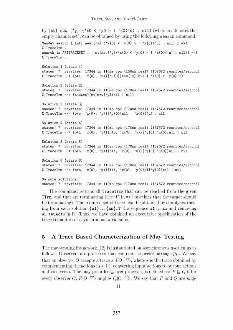
Thati, Sen, and Martı-Oliet

by [mt] new [’y] (’x0 < ’y0 > | ’x0(’u) . nil) (where mt denotes theempty channel set), can be obtained by using the following search command.

Maude> search [ [mt] new [’y] (’x0 < ’y0 > | ’x0(’u) . nil) ] =>!X:TraceTrm .search in APITRACESET : [[mt]new[’y](’x0 < ’y0 > | ’x0(’u) . nil)] =>!X:TraceTrm .

Solution 1 (state 1)states: 7 rewrites: 17344 in 110ms cpu (150ms real) (157672 rewrites/second)X:TraceTrm --> b(i, ’x0, ’u)[’u0]new[’y](nil | ’x0 < ’y0 >)

Solution 2 (state 2)states: 7 rewrites: 17344 in 110ms cpu (170ms real) (157672 rewrites/second)X:TraceTrm --> tauAct[mt]new[’y](nil | nil)

Solution 3 (state 3)states: 7 rewrites: 17344 in 110ms cpu (170ms real) (157672 rewrites/second)X:TraceTrm --> b(o, ’x0, ’y)[’y0]nil | ’x0(’u) . nil

Solution 4 (state 4)states: 7 rewrites: 17344 in 110ms cpu (170ms real) (157672 rewrites/second)X:TraceTrm --> b(i, ’x0, ’u)b(o, ’x0, ’y)[’y0 ’u0]nil | nil

Solution 5 (state 5)states: 7 rewrites: 17344 in 110ms cpu (170ms real) (157672 rewrites/second)X:TraceTrm --> b(o, ’x0, ’y)b(i, ’x0, ’u)[’y0 ’u0]nil | nil

Solution 6 (state 6)states: 7 rewrites: 17344 in 110ms cpu (170ms real) (157672 rewrites/second)X:TraceTrm --> b(o, ’x0, ’y)f(i, ’x0, ’y0)[’y0]nil | nil

No more solutions.states: 7 rewrites: 17344 in 110ms cpu (170ms real) (157672 rewrites/second)

The command returns all TraceTrms that can be reached from the givenTTrm, and that are terminating (the ‘!’ in =>! specifies that the target shouldbe terminating). The required set of traces can be obtained by simply extract-ing from each solution a1...anTT the sequence a1...an and removingall tauActs in it. Thus, we have obtained an executable specification of thetrace semantics of asynchronous π-calculus.

5 A Trace Based Characterization of May Testing

The may-testing framework [12] is instantiated on asynchronous π-calculus asfollows. Observers are processes that can emit a special message µµ. We say

that an observer O accepts a trace s if Os.µµ=⇒, where s is the trace obtained by

complementing the actions in s, i.e. converting input actions to output actionsand vice versa. The may preorder v over processes is defined as: P v Q if for

every observer O, P |O µµ=⇒ implies Q|O µµ

=⇒. We say that P and Q are may-

11

357

Thati, Sen, and Martı-Oliet

(Drop) s1.(y)s2 ≺ s1.(y)xy.s2 if (y)s2 6= ⊥(Delay) s1.(y)(α.xy.s2) ≺ s1.(y)xy.α.s2 if (y)(α.xy.s2) 6= ⊥

(Annihilate) s1.(y)s2 ≺ s1.(y)xy.xy.s2 if (y)s2 6= ⊥Table 3

A preorder relation on traces.

equivalent, i.e. P = Q, if P v Q and Q v P . The universal quantificationon contexts in this definition makes it very hard to prove equalities directlyfrom the definition, and makes mechanical checking impossible. To circumventthis problem, a trace based alternate characterization of the may equivalenceis proposed in [5]. We now summarize this characterization and discuss ourimplementation of it.

The preorder ¹ on traces is defined as the reflexive transitive closure ofthe laws shown in Table 3, where the notation (y)· is extended to traces asfollows.

(y)s =

s if y = ∅ or b 6∈ fn(s)

s1.x(y).s2 if y = y and there are s1, s2, x such that

s = s1.xy.s2 and y 6∈ n(s1) ∪ x⊥ otherwise

For sets of traces R and S, we define R - S, if for every s ∈ S there isan r ∈ R such that r ¹ s. The may preorder is then characterized in [5] as:P v Q if and only if [|Q|] - [|P |].

The main intuition behind the preorder ¹ is that if an observer acceptsa trace s, then it also accepts any trace r ¹ s. The first two laws state thatan observer cannot force inputs on the process being tested. Since outputsare asynchronous, the actions following an output in a trace exhibited by theobserver need not causally depend on the output. Hence the observer’s outputcan be delayed until a causally dependent action, or dropped if there are nosuch actions. The annihilation law states that an observer can consume itsown outputs unless there are subsequent actions that depend on the output.The reader is referred to [5] for further details on this characterization.

We encode the trace preorder as rewrite rules on terms of the sort TTraceof complete traces; specifically, the relation r ≺ s if cond, is encoded as s

=> r if cond. The reason for this form of representation will be justifiedin Section 6. The function (y)· on traces is defined equationally by theoperation bind. The constant bot of sort Trace is used by the bind operationto signal error.

op bind : Qid Trace -> Trace .op bot : -> Trace .var TR : Trace . var IO : ActionType.

12

358

Thati, Sen, and Martı-Oliet

ceq TR . bot = bot if t =/= epsilon .ceq bot . TR = bot if t =/= epsilon .

eq bind(X , epsilon) = epsilon .

eq bind(X , f(i,CX,CY) . TR ) = if CX =/= X0 thenif CY == X0 then ([shiftdown X] b(i, CX , X)) . TR

else ([shiftdown X] f(i, CX , CY)) . bind(X , TR) fielse bot fi .

eq bind(X , b(IO,CX,Y) . TR) = if CX =/= X0 thenif X =/= Y then ([shiftdown X] b(i, CX , Y)) . bind(X , TR)

else ([shiftdown X] b(IO, CX , Y)) . bind(X , swap(X,TR)) fielse bot fi .

The equation for the case where the second argument to bind begins witha free output is not shown as it is similar. Note that the channel indicesin actions until the first occurrence of X0 as the argument of a free inputare shifted down as these move out of the scope of the binder X. Further,when a bound action with X as the bound argument is encountered, the swap

operation is applied to the remaining suffix of the trace. The swap operationsimply changes the channel indices in the suffix so that the binding relationis unchanged even as the binder X is moved across the bound action. This isaccomplished by simultaneously substituting X0 with X1, and X1 withX0. Finally, note that when X0 is encountered as the argument of a freeinput, the input is converted to a bound input. If X0 is first encountered atany other place, an error is signalled by returning the constant bot.

The encoding of the preorder relation on traces is now straightforward.

crl [Drop] : [ TR1 . b(i,CX,Y) . TR2 ] => [ TR1 . bind(Y , TR2) ]if bind(Y , TR2) =/= bot .

rl [Delay] : [ ( TR1 . f(i,CX,CY) . b(IO,CU,V) . TR2 ) ] =>[ ( TR1 . b(IO,CU,V) . ([shiftup V] f(i, CX , CY)) . TR2 ) ] .

crl [Delay] : [ ( TR1 . b(i,CX,Y) . f(IO,CU,CV) . TR2 ) ] =>[ ( TR1 . bind(Y , f(IO,CU,CV) . f(i,CX,Y0) . TR2) ) ]

if bind(Y , f(IO,CU,CV) . f(i,CX,Y0) . TR2) =/= bot .

crl [Annihilate] : [ ( TR1 . b(i,CX,Y) . f(o,CX,Y0) . TR2 ) ] =>[ TR1 . bind(Y , TR2) ]

if bind(Y , TR2) =/= bot .

Note that in the first Delay rule, the channel indices of the free inputaction are shifted up when it is delayed across a bound action, since it getsinto the scope of the bound argument. Similarly, in the second Delay rule,when the bound input action is delayed across a free input/output action,the channel indices of the free action are shifted down by the bind operation.The other two subcases of the Delay rule, namely, where a free input is tobe delayed across a free input or output, and where a bound input is to bedelayed across a bound input or output, are not shown as they are similar.

13

359

Thati, Sen, and Martı-Oliet

Similarly, for Annihilate, the case where a free input is to be annihilatedwith a free output is not shown.

6 Verifying the May Preorder between Finite Processes

We now describe our implementation of verification of the may preorder be-tween finite processes, i.e. processes without replication, by exploiting thetrace-based characterization of may testing discussed in Section 5. The finite-ness of a process P only implies that the length of traces in [|P |] is bounded,but the number of traces in [|P |] can be infinite (even modulo α-equivalence)because the INP rule is infinitely branching. To avoid the problem of havingto compare infinite sets, we observe that

[|Q|] - [|P |] if and only if [|Q|]fn(P,Q) - [|P |]fn(P,Q),

where for a set of traces S and a set of names ρ we define Sρ = s ∈ S |fn(s) ⊆ ρ. Now, since the traces in [|P |] and [|Q|] are finite in length, itfollows that the sets of traces [|P |]fn(P,Q) and [|Q|]fn(P,Q) are finite modulo α-equivalence. In fact, the set of traces generated for [[fn(P,Q)] P] by ourimplementation described in Section 3, contains exactly one representativefrom each α-equivalence class of [|P |]fn(P,Q).

Given processes P and Q, we generate the set of all traces (modulo α-equivalence) of [[fn(P,Q)] P] and [[fn(P,Q)] Q] using the metalevel fa-cilities of Maude 2.0. As mentioned in Section 4, these terms, which areof sort TTrm, can be rewritten only once. The term of sort TraceTrm ob-tained by rewriting contains a finite trace as a prefix. To create the set of alltraces, we compute all possible one-step rewrites. This computation is done atthe metalevel by the function TTrmtoNormalTraceSet that uses two auxiliaryfunctions TTrmtoTraceSet and TraceSettoNormalTraceSet.

op TTrmtoTraceSet : Term -> TermSet .op TraceSettoNormalTraceSet : TermSet -> TermSet .op TTrmtoNormalTraceSet : Term -> TermSet .

eq TTrmtoNormalTraceSet(T) = TraceSettoNormalTraceSet(TTrmtoTraceSet(T)) .

The function TTrmTraceSet uses the function allOneStepAux(T,N) thatreturns the set of all one-step rewrites (according to the rules in Sections 3and 4, which are defined in modules named APISEMANTICS and APITRACE, seeFigure A.1 in appendix) of the term T which is the metarepresentation of aterm of sort TTrm, skipping the first N solutions. In the following equations,the operator u stands for set union.

Notice the use of the operation metaSearch, which receives as argumentsthe metarepresented module to work in, the starting term for search, thepattern to search for, a side condition (empty in this case), the kind of search(which may be ’* for zero or more rewrites, ’+ for one or more rewrites, and’! for only matching normal forms), the depth of search, and the requiredsolution number. It returns the term matching the pattern, its type, and

14

360

Thati, Sen, and Martı-Oliet

the substitution produced by the match; to keep only the term, we use theprojection getTerm.

op APITRACE-MOD : -> Module .eq APITRACE-MOD = [’APITRACE] .var N : MachineInt . vars T X : Term .

op allOneStepAux : Term MachineInt Term -> TermSet .op TraceTermToTrace : Term -> Term .

eq TTrmtoTraceSet(T) = allOneStepAux(T,0,’X:TraceTrm) .eq allOneStepAux(T,N,X) =

if metaSearch(APITRACE-MOD,T,X,nil,’+,1,N) == failurethen ’epsilon.Traceelse TraceTermToTrace(getTerm(metaSearch(APITRACE-MOD,T,X,nil,’+,1,N)))

u allOneStepAux(T,N + 1,X) fi .

The function TraceTrmToTrace (whose equations are not shown), usedin allOneStepAux, extracts the trace a1.a2...an out of a metarepresenta-tion of a term of sort TraceTrm of the form a1a2...anTT. The functionTraceSettoNormalTraceSet uses the metalevel operation metaReduce to con-vert each trace in a trace set to its α-normal form. The operation metaReduce

takes as arguments a metarepresented module and a metarepresented termin that module, and returns the metarepresentation of the fully reduced formof the given term using the equations in the given module, together with itscorresponding sort or kind. Again, the projection getTerm leaves only theresulting term.

eq TraceSettoNormalTraceSet(mt) = mt .eq TraceSettoNormalTraceSet(T u TS) =

getTerm(metaReduce(TRACE-MOD,’‘[_‘] [ T ]))u TraceSettoNormalTraceSet(TS) .

We implement the relation - on sets defined in Section 5 as the predicate<<. We check if P v Q by computing this predicate on the metarepresentedtrace sets [|P |]fn(P,Q) and [|Q|]fn(P,Q) as follows. For each (metarepresented)trace T in [|P |]fn(P,Q), we compute the reflexive transitive closure of T withrespect to the laws shown in Table 3. The laws are implemented as rewriterules in the module TRACE-PREORDER. We then use the fact that [|Q|]fn(P,Q) -[|P |]fn(P,Q) if and only if for every trace T in [|P |]fn(P,Q) the closure of T and[|Q|]fn(P,Q) have a common element.

op TRACE-PREORDER-MOD : -> Module .eq TRACE-PREORDER-MOD = [’TRACE-PREORDER] .var N : MachineInt . vars T T1 T2 X : Term .var TS TS1 TS2 : TermSet .

op _<<_ : TermSet TermSet -> Bool .op _<<<_ : TermSet Term -> Bool .op TTraceClosure : Term -> TermSet .op TTraceClosureAux : Term Term MachineInt -> TermSet .op _maypre_ : Term Term -> Bool .

15

361

Thati, Sen, and Martı-Oliet

eq TS2 << mt = true .eq TS2 << (T1 u TS1) = TS2 <<< T1 and TS2 << TS1 .eq TS2 <<< T1 = not disjoint?(TS2 , TTraceClosure(T1)) .eq T1 maypre T2 = TTrmtoNormalTraceSet(T2) << TTrmtoNormalTraceSet(T1) .

The computation of the closure of T is done by the function TTraceClosure.It uses TTraceClosureAux to compute all possible (multi-step) rewrites of theterm T using the rules defined in the module TRACE-PREORDER, again by meansof the metalevel operation metaSearch.

eq TTraceClosure(T) = TTraceClosureAux(T,’TT:TTrace,0) .eq TTraceClosureAux(T,X,N) =

if metaSearch(TRACE-PREORDER-MOD,T,X,nil,’*,maxMachineInt,N) == failurethen mtelse getTerm(metaSearch(TRACE-PREORDER-MOD,T,X,nil,’*,maxMachineInt,N))

u TTraceClosureAux(T,X,N + 1) fi .

This computation is terminating as the number of traces to which a tracecan rewrite using the trace preorder laws is finite modulo α-equivalence. Thisfollows from the fact that the length of a trace is non-increasing across rewrites,and the free names in the target of a rewrite are also free names in the source.Since the closure of a trace is finite, metaSearch can be used to enumerate allthe traces in the closure. Note that although the closure of a trace is finite, itis possible to have an infinite rewrite that loops within a subset of the closure.Further, since T is a metarepresentation of a trace, metaSearch can be applieddirectly to T inside the function TTraceClosureAux(T,X,N).

We end this section with a small example, which checks for the may-testingpreorder between the processes P = a(u).b(v).(νw)(wv|au)+b(u).a(v).(bu|bw)and Q = b(u).(bu|bw). We define constants TP and TQ of sort TTrm, along withthe following equations:

eq TP = [[’a0 ’b0 ’w0]’a0(’u) . ’b0(’v) . new[’w](’w0 < ’v0 > | ’a0 < ’u0 >)

+ ’b0(’u) . ’a0(’v) . (’b0 < ’u0 > | ’b0 < ’w0 >)]

eq TQ = [[’a0 ’b0 ’w0]’b0(’u) . (’b0 < ’u0 > | ’b0 < ’w0 >)]

The metarepresentation of these TTrms can now be obtained by using’TP.TTrm and ’TQ.TTrm, and we can then check for the may-testing preorderbetween the given processes as follows:

Maude> red ’TP.TTrm maypre ’TQ.TTrm .reduce in APITRACESET : ’TP.TTrm maypre ’TQ.TTrm .rewrites: 791690 in 2140ms cpu (2160ms real) (361422 rewrites/second)result Bool: trueMaude> red ’TQ.TTrm maypre ’TP.TTrm .reduce in APITRACESET : ’TQ.TTrm maypre ’TP.TTrm .rewrites: 664833 in 1620ms cpu (1640ms real) (410390 rewrites/second)result Bool: false

Thus, we have P v Q, but Q /v P . The reader can check that indeed,[|Q|]fn(P,Q) - [|P |]fn(P,Q), but [|P |]fn(P,Q) /- [|Q|]fn(P,Q).

16

362

Thati, Sen, and Martı-Oliet

7 Conclusions and Future Work

In this paper, we have described an executable specification in Maude of theoperational semantics of an asynchronous version of the π-calculus using con-ditional rewrite rules with rewrites in the conditions as proposed by Verdejoand Martı-Oliet in [18], and the CINNI calculus proposed by Stehr in [14]for managing names and their binding. In addition, we also implementedthe may-testing preorder for π-calculus processes using the Maude metalevel,where we use the metaSearch operation to calculate the set of all traces for aprocess and then compare two sets of traces according to a preorder relationbetween traces. As emphasized throughout the paper, the new features intro-duced in Maude 2.0 have been essential for the development of this executablespecification, including rewrites in conditions, the frozen attribute, and themetaSearch operation.

An interesting direction of further work is to extend our implementationto the various typed variants of π-calculus. Two specific typed asynchronousπ-calculi for which the work is under way are the local π-calculus (Lπ) [10]and the Actor model [1,15]. Both of these formal systems have been usedextensively in formal specification and analysis of concurrent object-orientedlanguages [2,8], and open distributed and mobile systems [9]. The alternatecharacterization of may testing for both of these typed calculi was recentlypublished [16,17]. We are extending the work presented here to account forthe type systems for these calculi, and modifications to the trace based char-acterization of may testing. We are also looking for interesting concrete appli-cations to which this can be applied; such experiments may require extendingour implementation to extensions of π-calculus with higher level constructs,although these may just be syntactic sugar.

Acknowledgements

This research has been supported in part by the Defense Advanced ResearchProjects Agency (contract numbers F30602-00-2-0586 and F33615-01-C-1907),the ONR MURI Project A Logical Framework for Adaptive System Inter-operability, and the Spanish CICYT project Desarrollo Formal de SistemasBasados en Agentes Moviles (TIC2000–0701–C02–01). This work was donewhile the last author was visiting the Department of Computer Science inthe University of Illinois at Urbana-Champaign, for whose hospitality he isvery grateful. We would like to thank Jose Meseguer for encouraging us toput together several complementary lines of work in order to get the resultsdescribed in this paper.

References

[1] G. Agha. Actors: A Model of Concurrent Computation in Distributed Systems.MIT Press, 1986.

17

363

Thati, Sen, and Martı-Oliet

[2] G. Agha. Concurrent object-oriented programming. Communications of theACM, 33(9):125–141, September 1990.

[3] M. Boreale and R. De Nicola. Testing equivalence for mobile processes.Information and Computation, 120:279–303, 1995.

[4] M. Boreale, R. De Nicola, and R. Pugliese. Proof techniques for cryptographicprocesses. In Proceedings 14th IEEE Symposium on Logic in Computer Science,LICS’99, Trento, Italy, July 2–5, 1999, pages 157–166. IEEE Computer SocietyPress, 1999.

[5] M. Boreale, R. De Nicola, and R. Pugliese. Trace and testing equivalence onasynchronous processes. Information and Computation, 172(2):139–164, 2002.

[6] P. Borovansky, C. Kirchner, H. Kirchner, P.-E. Moreau, and M. Vittek.ELAN: A logical framework based on computational systems. In J. Meseguer,editor, Proceedings First International Workshop on Rewriting Logic and itsApplications, WRLA’96, Asilomar, California, September 3–6, 1996, volume 4of Electronic Notes in Theoretical Computer Science, pages 35–50. Elsevier,1996. http://www.elsevier.nl/locate/entcs/volume4.html.

[7] M. Clavel, F. Duran, S. Eker, P. Lincoln, N. Martı-Oliet, J. Meseguer, and J.F. Quesada. Towards Maude 2.0. In K. Futatsugi, editor, Proceedings ThirdInternational Workshop on Rewriting Logic and its Applications, WRLA 2000,Kanazawa, Japan, September 18–20, 2000, volume 36 of Electronic Notes inTheoretical Computer Science, pages 297–318. Elsevier, 2000. http://www.elsevier.nl/locate/entcs/volume36.html.

[8] I. A. Mason and C. Talcott. A semantically sound actor translation. InP. Degano, R. Gorrieri, and A. Marchetti-Spaccamela, editors, Automata,Languages and Programming, 24th International Colloquium, ICALP’97,Bologna, Italy, July 7–11, 1997, Proceedings, volume 1256 of Lecture Notesin Computer Science, pages 369–378. Springer-Verlag, 1997.

[9] M. Merro, J. Kleist, and U. Nestmann. Local π-calculus at work: Mobile objectsas mobile processes. In J. van Leeuwen et al., editors, Theoretical ComputerScience: Exploring New Frontiers of Theoretical Informatics, InternationalConference IFIP TCS 2000 Sendai, Japan, August 17–19, 2000, Proceedings,volume 1872 of Lecture Notes in Computer Science, pages 390–408. Springer-Verlag, 2000.

[10] M. Merro and D. Sangiorgi. On asynchrony in name-passing calculi. InK. G. Larsen, S. Skyum, and G. Winskel, editors, Automata, Languages andProgramming, 25th International Colloquium, ICALP’98, Aalborg, Denmark,July 13–17, 1998, Proceedings, volume 1443 of Lecture Notes in ComputerScience, pages 856–867. Springer-Verlag, 1998.

[11] R. Milner, J. Parrow, and D. Walker. A calculus of mobile processes (Parts Iand II). Information and Computation, 100:1–77, 1992.

[12] R. De Nicola and M. Hennessy. Testing equivalence for processes. TheoreticalComputer Science, 34:83–133, 1984.

18

364

Thati, Sen, and Martı-Oliet

[13] G. D. Plotkin. A structural approach to operational semantics. TechnicalReport DAIMI FN-19, Computer Science Dept., Aarhus University, September1981.

[14] M.-O. Stehr. CINNI — A generic calculus of explicit substitutions and itsapplication to λ-, ς- and π-calculi. In K. Futatsugi, editor, Proceedings ThirdInternational Workshop on Rewriting Logic and its Applications, WRLA 2000,Kanazawa, Japan, September 18–20, 2000, volume 36 of Electronic Notes inTheoretical Computer Science, pages 71–92. Elsevier, 2000. http://www.elsevier.nl/locate/entcs/volume36.html.

[15] C. Talcott. An actor rewriting theory. In J. Meseguer, editor, Proceedings FirstInternational Workshop on Rewriting Logic and its Applications, WRLA’96,Asilomar, California, September 3–6, 1996, volume 4 of Electronic Notes inTheoretical Computer Science, pages 360–383. Elsevier, 1996. http://www.elsevier.nl/locate/entcs/volume4.html.

[16] P. Thati, R. Ziaei, and G. Agha. A theory of may testing for actors. In B. Jacobsand A. Rensink, editors, Proceedings IFIP TC6/WG6.1 Fifth InternationalConference on Formal Methods for Open Object-Based Distributed Systems(FMOODS 2002), March 20-22, 2002, Enschede, The Netherlands, pages 147–162. Kluwer Academic Publishers, 2002.

[17] P. Thati, R. Ziaei, and G. Agha. A theory of may testing for asynchronouscalculi with locality and no name matching. In H. Kirchner and C. Ringeissen,editors, Algebraic Methodology and Software Technology, 9th InternationalConference, AMAST 2002, Saint-Gilles-les-Bains, Reunion Island, France,September 9-13, 2002, Proceedings, volume 2422 of Lecture Notes in ComputerScience. Springer-Verlag, 2002.

[18] A. Verdejo and N. Martı-Oliet. Implementing CCS in Maude 2. In U.Montanari, editor, Proceedings Fourth International Workshop on RewritingLogic and its Applications, WRLA 2002, Pisa, Italy, September 19–21, 2002,volume 71 of Electronic Notes in Theoretical Computer Science. Elsevier, 2002.(This volume.) http://www.elsevier.nl/locate/entcs/volume71.html.

[19] P. Viry. Input/output for ELAN. In J. Meseguer, editor, Proceedings FirstInternational Workshop on Rewriting Logic and its Applications, WRLA’96,Asilomar, California, September 3–6, 1996, volume 4 of Electronic Notes inTheoretical Computer Science, pages 51–64. Elsevier, 1996. http://www.elsevier.nl/locate/entcs/volume4.html.

A Appendix

The diagram in Figure A.1 illustrates the graph of module importation in ourimplementation that closely follows the structure of the paper. The completecode is available at http://osl.cs.uiuc.edu/~ksen/api/. Here we onlyshow the module that contains the rewrite rules for the operational semantics

19

365

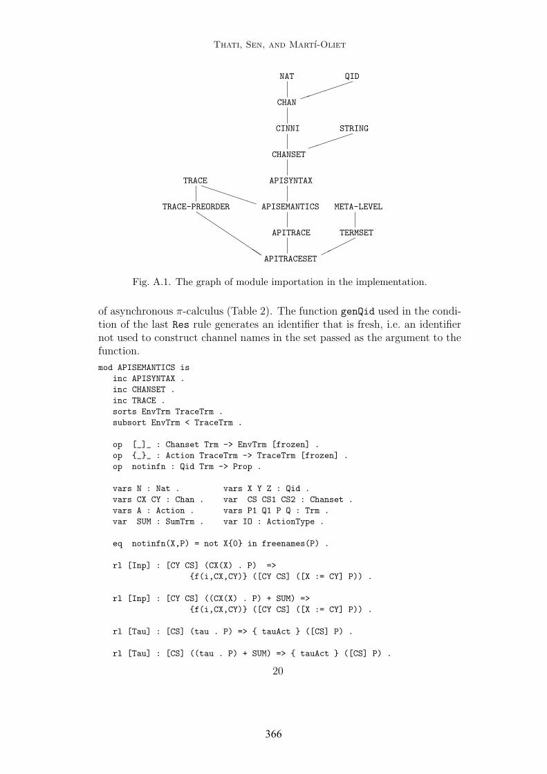
Thati, Sen, and Martı-Oliet

NAT QID³³³³³³

CHAN

CINNI STRING³³³³³

CHANSET

TRACEPPPPPP

APISYNTAX

TRACE-PREORDERQ

QQ

QQ

QQQ

APISEMANTICS META-LEVEL

APITRACE TERMSET©©©©

APITRACESET

Fig. A.1. The graph of module importation in the implementation.

of asynchronous π-calculus (Table 2). The function genQid used in the condi-tion of the last Res rule generates an identifier that is fresh, i.e. an identifiernot used to construct channel names in the set passed as the argument to thefunction.

mod APISEMANTICS isinc APISYNTAX .inc CHANSET .inc TRACE .sorts EnvTrm TraceTrm .subsort EnvTrm < TraceTrm .

op [_]_ : Chanset Trm -> EnvTrm [frozen] .op __ : Action TraceTrm -> TraceTrm [frozen] .op notinfn : Qid Trm -> Prop .

vars N : Nat . vars X Y Z : Qid .vars CX CY : Chan . var CS CS1 CS2 : Chanset .vars A : Action . vars P1 Q1 P Q : Trm .var SUM : SumTrm . var IO : ActionType .

eq notinfn(X,P) = not X0 in freenames(P) .

rl [Inp] : [CY CS] (CX(X) . P) =>f(i,CX,CY) ([CY CS] ([X := CY] P)) .

rl [Inp] : [CY CS] ((CX(X) . P) + SUM) =>f(i,CX,CY) ([CY CS] ([X := CY] P)) .

rl [Tau] : [CS] (tau . P) => tauAct ([CS] P) .

rl [Tau] : [CS] ((tau . P) + SUM) => tauAct ([CS] P) .

20

366

Thati, Sen, and Martı-Oliet

crl [BInp] : [CS] P => b(i,CX,’u) [’u0 [shiftup ’u] CS] P1if (not flag in CS) /\

CS1 := flag ’u0 [shiftup ’u] CS /\[CS1] [shiftup ’u] P => f(i,CX,’u0) [CS1] P1 .

rl [Out] : [CS] CX < CY > => f(o,CX,CY) ([CS] nil) .

crl [Par] : [CS] (P | Q) => f(IO,CX,CY) ([CS] (P1 | Q))if [CS] P => f(IO,CX,CY) ([CS] P1) .

crl [Par] : [CS] (P | Q) =>b(IO,CX,Y) [Y0 ([shiftup Y] CS)] (P1 | [shiftup Y] Q)

if [CS] P => b(IO,CX,Y) ([CS1] P1) .

crl [Com] : [CS] (P | Q) => tauAct ([CS] (P1 | Q1))if [CS] P => f(o,CX,CY) ([CS] P1) /\

[CY CS] Q => f(i,CX,CY) ([CY CS] Q1) .

crl [Close] : [CS] (P | Q) => tauAct [CS] new [Y] (P1 | Q1)if [CS] P => b(o,CX,Y) [CS1] P1 /\

[Y0 [shiftup Y] CS] [shiftup Y] Q =>f(i,CX,Y0) [CS2] Q1 .

crl [Res] : [CS] (new [X] P) =>[shiftdown X] f(IO,CX,CY) [CS] (new [X] P1)

if CS1 := [shiftup X] CS /\[CS1] P => f(IO,CX,CY) [CS1] P1 /\(not X0 in (CX CY)) .

crl [Res] : [CS] (new [X] P) => tauAct [CS] (new [X] P1)if [CS] P => tauAct [CS] P1 .

crl [Res] : [CS] (new [X] P) =>[shiftdown X] b(o,CX,Z) [Z0 CS] new[X]([ Y := Z0 ] P1)if Z := genQid(X0 CS freenames(P)) /\

[[shiftup X] CS] P => b(o,CX,Y) [CS1] P1 /\X0 =/= CX .

crl [Open] : [CS] (new[X] P) => [shiftdown X] b(o,CY,X) [X0 CS1] P1if CS1 := [shiftup X] CS /\

[CS1] P => f(o,CY,X0) [CS1] P1 /\ X0 =/= CY .

crl [If] : [CS1] (if CX = CX then P else Q fi) => A [CS2] P1if [CS1] P => A [CS2] P1 .

crl [Else] : [CS1] (if CX = CY then P else Q fi) => A [CS2] Q1if CX =/= CY /\ [CS1] Q => A [CS2] Q1 .

crl [Rep] : [CS1] (! P) => A [CS2] P1if [CS1] (P | (! P)) => A [CS2] P1 .

endm

21

367

Generating Optimal Linear Temporal LogicMonitors by Coinduction

Koushik Sen, Grigore Rosu, Gul AghaDepartment of Computer Science,

University of Illinois at Urbana-Champaign.ksen,grosu,agha@cs.uiuc.edu

Abstract. A coinduction-based technique to generate an optimal mon-itor from a Linear Temporal Logic (LTL) formula is presented in thispaper. Such a monitor receives a sequence of states (one at a time) froma running process, checks them against a requirements specification ex-pressed as an LTL formula, and determines whether the formula hasbeen violated or validated. It can also say whether the LTL formulais not monitorable any longer, i.e., that the formula can in the futureneither be violated nor be validated. A Web interface for the presentedalgorithm adapted to extended regular expressions is available.

1 IntroductionLinear Temporal Logic (LTL) [19] is a widely used logic for specifying propertiesof reactive and concurrent systems. The models of LTL are infinite executiontraces, reflecting the behavior of such systems as ideally always being readyto respond to requests, operating system being typical example. LTL has beenmainly used to specify properties of finite-state reactive and concurrent systems,so that the full correctness of the system can be verified automatically, usingmodel checking or theorem proving. Model checking of programs has received anincreased attention from the formal methods community within the last coupleof years, and several tools have emerged that directly model check source codewritten in Java or C [7, 26, 27]. Unfortunately, such formal verification techniquesare not scalable to real-sized systems without exerting a substantial effort toabstract the system more or less manually to a model that can be analyzed.

Testing scales well, and in practice it is by far the technique most used tovalidate software systems. Our approach follows research which merges testingand temporal logic specification in order to achieve some of the benefits of bothapproaches; we avoid some of the pitfalls of ad hoc testing as well as the com-plexity of full-blown theorem proving and model checking. While this mergerprovides a scalable technique, it does result in a loss of coverage: the techniquemay be used to examine a single execution trace at a time, and may not be usedto prove a system correct. Our work is based on the observation that softwareengineers are willing to trade coverage for scalability, so our goals is relativelyconservative: we provide tools that use formal methods in a lightweight manner,use traditional programming languages or underlying executional engines (suchas JVMs), are completely automatic, implement very efficient algorithms, andcan help find many errors in programs.

Recent trends suggest that the software analysis community is interestedin scalable techniques for software verification. Earlier work by Havelund and

368

Rosu [10] proposed a method based on merging temporal logics and testing.The Temporal Rover tool (TR) and its successor DB Rover by Drusinsky [2]have been commercialized. These tools instrument the Java code so that it cancheck the satisfaction of temporal logic properties at runtime. The MaC tool byLee et al. [14, 17] has been developed to monitor safety properties in intervalpast time temporal logic. In works by O’Malley et al. and Richardson et al. [20,21], various algorithms to generate testing automata from temporal logic formu-lae, are described. Java PathExplorer [8] is a runtime verification environmentcurrently under development at NASA Ames. It can analyze a single executiontrace. The Java MultiPathExplorer tool [25] proposes a technique to monitor allequivalent traces that can be extracted from a given execution, thus increasingthe coverage of monitoring. Giannakopoulou et al. and Havelund et al. in [4, 9]propose efficient algorithms for monitoring future time temporal logic formulae,while Havelund et al. in [11] gives a technique to synthesize efficient monitorsfrom past time temporal formulae. Rosu et al. in [23] shows use of rewritingto perform runtime monitoring of extended regular expressions. An approachsimilar to this paper is used to generate optimal monitors for extended regularexpressions in work by Sen et al. [24].

In this paper, we present a new technique based on the modern coalgebraicmethod to generate optimal monitors for LTL formulae. In fact, such monitorsare the minimal deterministic finite automata required to do the monitoring. Ourcurrent work makes two major contributions. First, we give a coalgebraic formal-ization of LTL and show that coinduction is a viable and reasonably practicalmethod to prove monitoring-equivalences of LTL formulae. Second, building onthe coinductive technique, we present an algorithm to directly generate mini-mal deterministic automata from an LTL formula. Such an automaton may beused to monitor good or bad prefixes of an execution trace (this notion will berigorously formalized in subsequent sections).

We describe the monitoring as synchronous and deterministic to obtain min-imal good or bad prefixes. However, if the cost of such monitoring is deemed toohigh in some application, and one is willing to tolerate some delay in discoveringviolations, the same technique could be applied on the traces intermittently –in which case one would not get minimal good or bad prefixes but could eitherbound the delay in discovering violations, or guarantee eventual discovery. Wealso give lower and upper bounds on the size of such automata.

The closely related work by Geilen [3] builds monitors to detect a subclassof bad and good prefixes, which are called informative bad and good prefixes.Using a tableau-based technique, [3] can generate monitors of exponential sizefor informative prefixes. In our approach, we generate minimal monitors fordetecting all kinds of bad and good prefixes. This generality comes at a price:the size of our monitors can be doubly exponential in the worst case, and thiscomplexity cannot be avoided.

One standard way to generate an optimal monitor is to use the Buchi au-tomata construction [16] for LTL to generate a non-deterministic finite automa-ton, determinize it and then to minimize it. In this method, one checks only

369

the syntactic equivalence of LTL formulae. In the coalgebraic technique that wepropose as an alternative method, we make use of the monitoring equivalence(defined in subsequent sections) of LTL formulae. We thus obtain the minimalautomaton in a single go and minimize the usage of computational space. More-over, our technique is completely based on deductive methods and can be appliedto any logic or algebra for which there is a suitable behavioral specification. Arelated application can be found in [24] in which the minimal deterministic finiteautomata for extended regular expressions is generated.

2 Linear Temporal Logic and DerivativesIn order to make the paper self-contained, we briefly describe classical LinearTemporal Logic over infinite traces. We use the classical definition of LinearTemporal Logic and assume a finite set AP of atomic propositions. The syntaxof LTL is as follows:

φ ::= true | false | a ∈ AP | ¬φ | φ ∧ φ | φ ∨ φ | φ → φ | φ ≡ φ | φ⊕ φ propositionalφ U φ | dφ | ¤φ | ♦φ temporal

The semantics of LTL is given for infinite traces. An infinite trace is an infinitesequence of program states, each state denoting the set of atomic propositionsthat hold at that state. The atomic propositions that hold in a given state s isgiven by AP (s). We denote an infinite trace by ρ; ρ(i) denotes the i-th state inthe trace and ρi denotes the suffix of the trace ρ starting from the i-th state.The notion that an infinite trace ρ satisfies a formula φ is denoted by ρ |= φ,and is defined inductively as follows:

ρ |= true for all ρ ρ 2 false for all ρρ |= a iff a ∈ AP (ρ(1)) ρ |= ¬φ iff ρ 2 φρ |= φ1 ∨ φ2 iff ρ |= φ1 or ρ |= φ2 ρ |= φ1 ∧ φ2 iff ρ |= φ1 and ρ |= φ2

ρ |= φ1 ⊕ φ2 iff ρ |= φ1 exclusive or ρ |= φ2 ρ |= φ1 → φ2 iff ρ |= φ1 implies ρ |= φ2

ρ |= φ1 ≡ φ2 iff ρ |= φ1 iff ρ |= φ2 ρ |= dφ iff ρ2 |= φρ |= ¤φ iff ∀ j ≥ 1 ρj |= φ ρ |= ♦φ iff ∃ j ≥ 1 such that ρj |= φρ |= φ1 U φ2 iff there exists a j ≥ 1 such that ρj |= φ2 and ∀ 1 ≤ i < j : ρi |= φ1

The set of all infinite traces that satisfy the formula φ is called the languageexpressed by the formula φ and is denoted by Lφ. Thus, ρ ∈ Lφ if and only ifρ |= φ. The language Lφ is also called the property expressed by the formula φ.We informally say that an infinite trace ρ satisfies a property φ iff ρ |= φ.

A property in LTL can be seen as the intersection of a safety property anda liveness property [1]. A property is a liveness property if for every finite traceα there exists an infinite trace ρ such that α.ρ satisfies the property. A propertyis a safety property if for every infinite trace ρ not satisfying the property, thereexists a finite prefix α such that for all infinite traces ρ′, α.ρ′ does not satisfythe property. The prefix α is called a bad prefix [3]. Thus, we say that a finiteprefix α is a bad prefix for a property if for all infinite traces ρ, α.ρ does notsatisfy the property. On the other hand, a good prefix for a property is a prefixα such that for all infinite traces ρ, α.ρ satisfies the property. A bad or a goodprefix can also be minimal. We say that a bad (or a good prefix) α is minimal ifα is a bad (or good) prefix and no finite prefix α′ of α is bad (or good) prefix.

370

We use a novel coinduction-based technique to generate an optimal monitorthat can detect good and bad prefixes incrementally for a given trace. The es-sential idea is to process, one by one, the states of a trace as these states aregenerated; at each step the process checks if the finite trace that we have alreadygenerated is a minimal good prefix or a minimal bad prefix. At any point, if wefind that the finite trace is a minimal bad prefix, we say that the property isviolated. If the finite trace is a minimal good prefix then we stop monitoring forthat particular trace and say that the property holds for that trace.

At any step, we will also detect if it is not possible to monitor a formula anylonger. We may stop monitoring at that point and say the trace is no longermonitorable and save the monitoring overhead. Otherwise, we continue by pro-cessing one more state and appending that state to the finite trace. We will seein the subsequent sections that these monitors can report a message as soon asa good or a bad prefix is encountered; therefore, the monitors are synchronous.Two more variants of the optimal monitor are also proposed; these variants canbe used to efficiently monitor either bad prefixes or good prefixes (rather thanboth). Except in degenerate cases, such monitors have smaller sizes than themonitors that can detect both bad and good prefixes.

In order to generate the minimal monitor for an LTL formula, we will useseveral notions of equivalence for LTL:Definition 1 (≡). We say that two LTL formulae φ1 and φ2 are equivalent i.e.φ1 ≡ φ2 if and only if Lφ1 = Lφ2 .Definition 2 (≡B). For a finite trace α we say that α 2 φ iff α is bad prefixfor φ i.e. for every infinite trace ρ it is the case that α.ρ 6∈ Lφ. Given two LTLformulae φ1 and φ2, φ1 and φ2 are said to be bad prefix equivalent i.e. φ1 ≡B φ2

if and only if for every finite trace α, α 2 φ1 iff α 2 φ2.Definition 3 (≡G). For a finite trace α we say that α |= φ iff α is good prefixfor φ i.e. for every infinite trace ρ it is that case that α.ρ ∈ Lφ. Given twoLTL formulae φ1 and φ2, φ1 and φ2 are said to be good prefix equivalent i.e.φ1 ≡G φ2 if and only if for every finite trace α, α |= φ1 iff α |= φ2.Definition 4 (≡GB). We say that φ1 and φ2 are good-bad prefix equivalenti.e. φ1 ≡GB φ2 if and only if φ1 ≡B φ2 and φ1 ≡G φ2.Thus, for our purpose, the two non equivalent formulae ¤♦φ and ♦¤φ are good-bad prefix equivalent since they do not have any good or bad prefixes. Suchformula are not monitorable. Note that the equivalence relation ≡ is includedin the equivalence relation ≡GB , which is in turn included in both ≡G and ≡B .We will use the equivalences ≡G ,≡B , and ≡GB to generate optimal monitorsthat detect good prefixes only, bad prefixes only and both bad and good prefixesrespectively. We call these three equivalences monitoring equivalences.

2.1 DerivativesWe describe the notion of derivatives for LTL [9, 10] based on the idea of stateconsumption: an LTL formula φ and a state s generate another LTL formula,denoted by φs, with the property that for any finite trace α, sα 2 φ if andonly if α 2 φs and sα |= φ if and only if α |= φs. We define the operator recursively through the following equations:

371

false s = false true s = trueps = if p ∈ AP (s) then true else false (¬φ)s = ¬(φs)(φ1 ∨ φ2)s = φ1s ∨ φ2s (φ1 ∧ φ2)s = φ1s ∧ φ2s(φ1 → φ2)s = φ1s → φ2s (φ1 ⊕ φ2)s = φ1s ⊕ φ2s(♦φ)s = φs ∨ ♦φ (¤φ)s = φs ∧¤φ(φ1 U φ2)s = φ2s ∨ (φ1s ∧ φ1 U φ2)

We use the decision procedure for propositional calculus by Hsiang [13] to get acanonical form for a propositional formula. The procedure reduces a tautologicalformula to the constant true, a false formula to the constant false, and all otherformulae to canonical forms modulo associativity and commutativity. An unusualaspect of this procedure is that the canonical forms consist of exclusive or (⊕)of conjunctions. The procedure is given below using equations that are shown tobe Church-Rosser and terminating modulo associativity and commutativity.

true ∧ φ = φ false ∧ φ = falseφ ∧ φ = φ false ⊕ φ = φφ⊕ φ = false ¬φ = true ⊕ φφ1 ∧ (φ2 ⊕ φ3) = (φ1 ∧ φ2)⊕ (φ1 ∧ φ3) φ1 ∨ φ2 = (φ1 ∧ φ2)⊕ φ1 ⊕ φ2

φ1 → φ2 = true⊕ φ1 ⊕ (φ1 ∧ φ2) φ1 ≡ φ2 = true⊕ φ1 ⊕ φ2

The exclusive or operator ⊕ and the ∧ operator are defined as commutativeand associative. The equations Derivative and Propositional Calculuswhen regarded as rewriting rules are terminating and Church-Rosser (moduloassociativity and commutativity of ∧ and ⊕), so they can be used as a functionalprocedure to calculate derivatives.

In the rest of the paper, at several places we need to check if an LTL formulais equivalent to true or false. This can be done using the tableau-based proofmethod for LTL; the STeP tool at Stanford [18] has such an implementation.

The following result gives a way to determine if a prefix is good or bad for aformula through derivations.Theorem 1. a) For any LTL formula φ and for any finite trace α = s1s2 . . . sn,α is a bad prefix for φ if and only if φs1s2 . . . sn ≡ false. Similarly, α isa good prefix for φ if and only if φs1s2 . . . sn ≡ true. b) The formulaφs1s2 . . . sn needs O(2size(φ)) space to be stored.Proof. b): Due to the Boolean ring equations above regarded as simplificationrules, any LTL formula is kept in a canonical form, which is an exclusive disjunc-tion of conjunctions, where conjuncts have temporal operators at top. Moreover,after a series of applications of derivatives s1, s2, ..., sn, the conjuncts in the nor-mal form φs1s2...sn are subterms of the initial formula φ, each having atemporal operator at its top. Since there are at most size(φ) such subformulae, itfollows that there are at most 2size(φ) possibilities to combine them in a conjunc-tion. Therefore, one needs space O(2size(φ)) to store any exclusive disjunction ofsuch conjunctions. This reasoning only applies on “idealistic” rewriting engines,which carefully optimize space needs during rewriting.utIn order to effectively generate optimal monitors, it is crucial to detect efficientlyand as early as possible when two derivatives are equivalent. In the rest ofthe paper we use coinductive techniques to solve this problem. We define the

372

operators G : LTL → true, false and B : LTL → true, false that returntrue if an LTL formula is equivalent (≡) to true or false respectively, and returnfalse otherwise. We define an operator GB : LTL → 0, 1, ? that checks if anLTL formula φ is equivalent to false or true and returns 0 or 1, respectively, andreturns ? if the formula is not equivalent to either true or false.

3 Hidden Logic and Coinduction

We use circular coinduction, defined rigorously in the context of hidden logicsand implemented in the BOBJ system [22, 5, 6], to test whether two LTL formu-lae are good-bad prefix equivalent. A particularly appealing aspect of circularcoinduction in the framework of LTL formula is that it not only shows that twoLTL formulae are good-bad prefix equivalent, but also generates a larger set ofgood-bad prefix equivalent LTL formulae which will all be used in order to gen-erate the target monitor. Readers familiar with circular coinduction may assumethe result in Theorem 4 and read Section 4 concurrently.

Hidden logic is a natural extension of algebraic specification which benefits ofa series of generalizations in order to capture various natural notions of behav-ioral equivalence found in the literature. It distinguishes visible sorts for datafrom hidden sorts for states, with states behaviorally equivalent if and only ifthey are indistinguishable under a formally given set of experiments. In order tokeep the presentation simple and self-contained, we define a simplified version ofhidden logic together with its associated circular coinduction proof rule which isnevertheless general enough to support the definition of LTL formulae and provethat they are behaviorally good and/or bad prefix equivalent.

3.1 Algebraic Preliminaries

We assume that the reader is familiar with basic equational logic and algebra butrecall a few notions in order to just make our notational conventions precise. AnS-sorted signature Σ is a set of sorts/types S together with operational symbolson those, and a Σ-algebra A is a collection of sets As | s ∈ S and a collectionof functions appropriately defined on those sets, one for each operational symbol.Given an S-sorted signature Σ and an S-indexed set of variables Z, let TΣ(Z)denote the Σ-term algebra over variables in Z. If V ⊆ S then Σ¹V is a V -sortedsignature consisting of all those operations in Σ with sorts entirely in V . Wemay let σ(X) denote the term σ(x1, ..., xn) when the number of arguments of σand their order and sorts are not important. If only one argument is important,then to simplify writing we place it at the beginning; for example, σ(t,X) is aterm having σ as root with no important variables as arguments except one, inthis case t. If t is a Σ-term of sort s′ over a special variable ∗ of sort s and A isa Σ-algebra, then At : As → As′ is the usual interpretation of t in A.

3.2 Behavioral Equivalence, Satisfaction and Specification

Given disjoint sets V, H called visible and hidden sorts, a hidden (V, H)-signature,say Σ, is a many sorted (V ∪H)-signature. A hidden subsignature of Σ is a hidden(V, H)-signature Γ with Γ ⊆ Σ and Γ¹V = Σ¹V . The data signature is Σ¹V . An

373

operation of visible result not in Σ¹V is called an attribute, and a hidden sortedoperation is called a method.

Unless otherwise stated, the rest of this section assumes fixed a hidden sig-nature Σ with a fixed subsignature Γ . Informally, Σ-algebras are universes ofpossible states of a system, i.e., “black boxes,” for which one is only concernedwith behavior under experiments with operations in Γ , where an experiment isan observation of a system attribute after perturbation.

A Γ -context for sort s ∈ V ∪H is a term in TΓ (∗ : s) with one occurrence of∗. A Γ -context of visible result sort is called a Γ -experiment. If c is a context forsort h and t ∈ TΣ,h then c[t] denotes the term obtained from c by substitutingt for ∗; we may also write c[∗] for the context itself.

Given a hidden Σ-algebra A with a hidden subsignature Γ , for sorts s ∈(V ∪H), we define Γ -behavioral equivalence of a, a′ ∈ As by a ≡Γ

Σ a′ iff Ac(a) =Ac(a′) for all Γ -experiments c; we may write ≡ instead of ≡Γ

Σ when Σ and Γcan be inferred from context. We require that all operations in Σ are compatiblewith ≡Γ

Σ . Note that behavioral equivalence is the identity on visible sorts, sincethe trivial contexts ∗ : v are experiments for all v ∈ V . A major result inhidden logics, underlying the foundations of coinduction, is that Γ -behavioralequivalence is the largest equivalence which is identity on visible sorts and whichis compatible with the operations in Γ .

Behavioral satisfaction of equations can now be naturally defined in termsof behavioral equivalence. A hidden Σ-algebra A Γ -behaviorally satisfies a Σ-equation (∀X) t = t′, say e, iff for each θ : X → A, θ(t) ≡Γ

Σ θ(t′); in this casewe write A |≡Γ

Σ e. If E is a set of Σ-equations we then write A |≡ΓΣ E when A

Γ -behaviorally satisfies each Σ-equation in E. We may omit Σ and/or Γ from|≡Γ

Σ when they are clear.A behavioral Σ-specification is a triple (Σ, Γ,E) where Σ is a hidden signa-

ture, Γ is a hidden subsignature of Σ, and E is a set of Σ-sentences equations.Non-data Γ -operations (i.e., in Γ − Σ¹V ) are called behavioral. A Σ-algebra Abehaviorally satisfies a behavioral specification B = (Σ, Γ,E) iff A |≡Γ

Σ E, inwhich case we write A |≡ B; also B |≡ e iff A |≡ B implies A |≡Γ

Σ e.LTL can be very naturally defined as a behavioral specification. The enor-

mous benefit of doing so is that the behavioral inference, including most impor-tantly coinduction, provide a decision procedure for good-bad prefix equivalence.

Example 1. A behavioral specification of LTL defines a set of two visible sortsV = Triple, State, one hidden sort H = Ltl, one behavioral attributeGB : Ltl → Triple (defined as an operator in Subsection 2.1) and one behavioralmethod, the derivative, : Ltl × State → Ltl , together with all the otheroperations in Section 2 defining LTL, including the states in S which are definedas visible constants of sort State, and all the equations in Subsection 2.1. Thesort Triple consists of three constants 0, 1, and ?. We call this the LTL behavioralspecification and we use BLTL/GB to denote it.

Since the only behavioral operators are the test for equivalence to true andfalse and the derivative, it follows that the experiments have exactly the formGB(∗s1s2...sn), for any states s1, s2, ..., sn. In other words, an experi-

374

ment consists of a series of derivations followed by an application of the operatorGB , and therefore two LTL formulae are behavioral equivalent if and only if theycannot be distinguished by such experiments. Such behavioral equivalence is ex-actly same as good-bad prefix equivalence. In the specification of BLTL/GB ifwe replace the attribute GB by B (or G), as defined in Subsection 2.1, the be-havioral equivalence becomes same as bad prefix (or good prefix) equivalence.We denote such specifications by BLTL/B (or BLTL/G). Notice that the abovereasoning applies within any algebra satisfying the presented behavioral specifi-cation. The one we are interested in is, of course, the free one, whose set carrierscontain exactly the LTL formulae as presented in Section 2, and the operationshave the obvious interpretations. We informally call it the LTL algebra.Letting ≡b denote the behavioral equivalence relation generated on the LTLalgebra, then Theorem 1 immediately yields the following important result.Theorem 2. If φ1 and φ2 are two LTL formulae then φ1 ≡b φ2 in BLTL/GB

iff φ1 and φ2 are good-bad prefix equivalent. Similarly, φ1 ≡b φ2 in BLTL/B (orBLTL/G) if and only if φ1 and φ2 are bad prefix (or good prefix) equivalent.This theorem allows us to prove good-bad prefix equivalence (or bad prefix orgood prefix equivalence) of LTL formulae by making use of behavioral inferencein the LTL behavioral specification BLTL/GB (or BLTL/B or BLTL/G) including(especially) circular coinduction. The next section shows how circular coinduc-tion works and how it can be used to show LTL formulae good-bad prefix equiv-alent (or bad prefix equivalent or good prefix equivalent). From now onwards wewill refer BLTL/GB simply by B.

3.3 Circular Coinduction as an Inference Rule

In the simplified version of hidden logics defined above, the usual equational in-ference rules, i.e., reflexivity, symmetry, transitivity, substitution and congruence[22] are all sound for behavioral satisfaction. However, equational reasoning canderive only a very limited amount of interesting behavioral equalities. For thatreason, circular coinduction has been developed as a very powerful automatedtechnique to show behavioral equivalence. We let ± denote the relation beingdefined by the equational rules plus circular coinduction, for deduction from aspecification to an equation.

Before formally defining circular coinduction, we give the reader some intu-itions by duality to structural induction. The reader who is only interested inusing the presented procedure or who is not familiar with structural induction,can skip this paragraph. Inductive proofs show equality of terms t(x), t′(x) overa given variable x (seen as a constant) by showing t(σ(x)) equals t′(σ(x)) forall σ in a basis, while circular coinduction shows terms t, t′ behaviorally equiv-alent by showing equivalence of δ(t) and δ(t′) for all behavioral operations δ.Coinduction applies behavioral operations at the top, while structural inductionapplies generator/constructor operations at the bottom. Both induction and cir-cular coinduction assume some “frozen” instances of t, t′ equal when checkingthe inductive/coinductive step: for induction, the terms are frozen at the bottomby replacing the induction variable by a constant, so that no other terms canbe placed beneath the induction variable, while for coinduction, the terms are

375

frozen at the top, so that they cannot be used as subterms of other terms (withsome important but subtle exceptions which are not needed here; see [6]).

Freezing terms at the top is elegantly handled by a simple trick. Supposeevery specification has a special visible sort b, and for each (hidden or visible)sort s in the specification, a special operation [ ] : s → b. No equations areassumed for these operations and no user defined sentence can refer to them;they are there for technical reasons. Thus, with just the equational inferencerules, for any behavioral specification B and any equation (∀X) t = t′, it isnecessarily the case that B ± (∀X) t = t′ iff B ± (∀X) [t] = [t′]. The rulebelow preserves this property. Let the sort of t, t′ be hidden; thenCircular Coinduction:B ∪ (∀X) [t] = [t′] ± (∀X, W ) [δ(t, W )] = [δ(t′, W )], for all appropriate δ ∈ Γ

B ± (∀X) t = t′

We call the equation (∀X) [t] = [t′] added to B a circularity; it could just aswell have been called a coinduction hypothesis or a co-hypothesis, but we find thefirst name more intuitive because from a coalgebraic point of view, coinductionis all about finding circularities.Theorem 3. The usual equational inference rules together with Circular Coin-duction are sound. That means that if B ± (∀X) t = t′ and sort(t, t′) 6= b, or ifB ± (∀X) [t] = [t′], then B |≡ (∀X) t = t′.Circular coinductive rewriting[5, 6] iteratively rewrites proof tasks to their normalforms followed by an one step coinduction if needed. Since the rules in BLTL/GB ,BLTL/B , and BLTL/G are ground Church-Rosser and terminating, this providesus with a decision procedure for good-bad prefix equivalence, bad prefix equiv-alence, and good prefix equivalence of LTL formulae respectively.Theorem 4. If φ1 and φ2 are two LTL formulae, then φ1 ≡GB φ2 if and onlyif BLTL/GB ± φ1 = φ2. Similarly, if φ1 and φ2 are two LTL formulae, thenφ1 ≡B φ2 (or φ1 ≡G φ2) if and only if BLTL/B ± φ1 = φ2 ( or BLTL/G ±φ1 = φ2). Moreover, circular coinductive rewriting provides us with a decisionprocedure for good-bad prefix equivalence, bad prefix equivalence, and good prefixequivalence of LTL formulae.Proof. By soundness of behavioral reasoning (Theorem 3), one implication fol-lows immediately via Theorem 2. For the other implication, assume that φ1 andφ2 are good-bad prefix equivalent (or good prefix or bad prefix equivalent, respec-tively) and that the equality φ1 = φ2 is not derivable from BLTL/GB (or BLTL/G

or BLTL/B , respectively). By Theorem 1, the number of formulae into whichany LTL formula can be derived via a sequence of events is finite, which meansthat the total number of equalities φ′1 = φ′2 that can be derived via the circularcoinduction rule is also finite. That implies that the only reason for which theequality φ1 = φ2 cannot be proved by circular coinduction is because it is in factdisproved by some experiment, which implies the existence of some events a1,..., an such that GB(φ1a1 · · · an) 6= GB(φ2a1 · · · an) (or the equivalentones for B or G). However, this is obviously a contradiction because if φ1 andφ2 are good-bad (or good or bad) prefix equivalent that so are φ1a1 · · · anand φ2a1 · · · an, and GB (or G or B) preserve this equivalence.

376

4 Generating Optimal Monitors by Coinduction

We now show how one can use the set of circularities generated by applyingthe circular coinduction rules in order to generate, from any LTL formula, anoptimal monitor that can detect both good and bad prefixes. The optimal mon-itor thus generated will be a minimal deterministic finite automaton containingtwo final states true and false. We call such a monitor GB-automaton. We con-clude the section by modifying the algorithm to generate smaller monitors thatcan detect either bad or good prefixes. We call such monitors B-automaton andG-automaton respectively. The main idea behind the algorithm is to associatestates in GB-automaton to LTL formulae obtained by deriving the initial LTLformula; when a new LTL formula is generated, it is tested for good-bad pre-fix equivalence with all the other already generated LTL formulae by using thecoinductive procedure presented in the previous section. A crucial observationwhich significantly reduces the complexity of our procedure is that once a good-bad prefix equivalence is proved by circular coinductive rewriting, the entire setof circularities accumulated represent good-bad prefix equivalent LTL formu-lae. These can be used to quickly infer the other good-bad prefix equivalences,without having to generate the same circularities over and over again.

Since BOBJ does not (yet) provide any mechanism to return the set of circu-larities accumulated after proving a given behavioral equivalence, we were unableto use BOBJ to implement our optimal monitor generator. Instead, we have im-plemented our own version of coinductive rewriting engine for LTL formulae,which is described below.

We are given an initial LTL formula φ0 over atomic propositions P . Thenσ = 2P is the set of possible states that can appear in an execution trace; notethat σ will be the set of alphabets in the GB-automaton. Now, from φ0 we wantto generate a GB-automaton D = (S, σ, δ, s0, true, false), where S is the set ofstates of the GB-automaton, δ : S × σ → S is the transition function, s0 is theinitial state of the GB-automaton, and true, false ⊆ S is the set of final statesof the DFA. The coinductive rewriting engine explicitly accumulates the provencircularities in a set. The set is initialized to an empty set at the beginning of thealgorithm. It is updated with the accumulated circularities whenever we provegood-bad prefix equivalence of two LTL formulae in the algorithm. The algorithmmaintains the set of states S in the form of non good-bad prefix equivalent LTLformulae. At the beginning of the algorithm S is initialized with two elements,the constant formulae true and false. Then, we check if the initial LTL formulaφ0 is equivalent to true or false. If φ0 is equivalent to true or false, we set s0 totrue or false respectively and return D as the GB-automaton. Otherwise, we sets0 to φ0, add φ0 to the set S, and invoke the procedure dfs (see Fig 1) on φ0.

The procedure dfs generates the derivatives of a given formula φ for allx ∈ σ one by one. A derivative φx = φx is added to the set S, if the set doesnot contain any LTL formula good-bad prefix equivalent to the derivative φx.We then extend the transition function by setting δ(φ, x) = φx and recursivelyinvoke dfs on φx. On the other hand, if an LTL formula φ′ equivalent to thederivative already exists in the set S, we extend the transition function by setting

377

δ(φ, x) = φ′. To check if an LTL formula, good-bad prefix equivalent to thederivative φx, already exists in the set S, we sequentially go through all theelements of the set S and try to prove its good-bad prefix equivalence with φx. Intesting the equivalence we first add the set of circularities to the initial BLTL/GB .Then we invoke the coinductive procedure. If for some LTL formula φ′ ∈ S, weare able to prove that φ′ ≡GB φx i.e BLTL/GB∪Eqall∪Eqnew ± φ′ = φx , then weadd the new equivalences Eqnew, created by the coinductive procedure, to the setof circularities. Thus we reuse the already proven good-bad prefix equivalencesin future proofs.

S ← true, falsedfs(φ)begin

foreach x ∈ σ doφx ← φx;if ∃φ′ ∈ S such that BLTL/GB ∪ Eqall ∪ Eqnew ± φ′ = φx then

δ(φ, x) = φ′; Eqall ← Eqall ∪ Eqnew

else S ← S ∪ φx; δ(φ, x) = φx; dfs(φx); fiendfor

end

Fig. 1. LTL to optimal monitor generation algorithm

The GB-automaton generated by the procedure dfs may now contain some stateswhich are non-final and from which the GB-automaton can never reach a finalstate. We remove these redundant states by doing a breadth first search in back-ward direction from the final states. This can be done in time linear in the sizeof the GB-automaton. If the resultant GB-automaton contains the initial states0 then we say that the LTL formula is monitorable. That is for the LTL formulato be monitorable there must be path from the initial state to a final state i.e.to true or false state. Note that the GB-automaton may now contain non-finalstates from which there may be no transition for some x ∈ σ. Also note that notransitions are possible from the final states.

The correctness of the algorithm is given by the following theorem.

Theorem 5. If D is the GB-automaton generated for a given LTL formula φby the above algorithm then1) L(D) is the language of good and bad prefixes of φ,2) D is the minimal deterministic finite automaton accepting the good and bad

prefixes of φ.

Proof. 1) Suppose s1s2 . . . sn be a good or bad prefix of φ. Then by Theorem1, GB(φs1s2 . . . sn) ∈ 0, 1. Let φi = φs1s2 . . . si; then φi+1 =φiai+1. To prove that s1s2 . . . sn ∈ L(D), we use induction to show that foreach 1 ≤ i ≤ n, φi ≡GB δ(φ, s1s2 . . . si). For the base case if φ1 ≡GB φs1 thendfs extends the transition function by setting δ(φ, s1) = φ. Therefore, φ1 ≡GB

φ = δ(φ, s1). If φ1 6≡GB φ then dfs extends δ by setting δ(φ, s1) = φ1. So φ1 ≡GB

δ(φ, s1) holds in this case also. For the induction step let us assume that φi ≡GB

φ′ = δ(φ, s1s2 . . . si). If δ(φ′, si+1) = φ′′ then from the dfs procedure we can see

378

that φ′′ ≡GB φ′si+1. However, φisi+1 ≡GB φ′si+1, since φi ≡GB φ′ byinduction hypothesis. So φi+1 ≡GB φ′′ = δ(φ′, si+1) = δ(φ, s1s2 . . . si+1). Alsonotice GB(φn ≡GB δ(φ, s1s2 . . . sn)) ∈ 0, 1; this implies that δ(φ, s1s2 . . . sn)is a final state and hence s1s2 . . . sn ∈ L(D).

Now suppose s1s2 . . . sn ∈ L(D). The proof that s1s2 . . . sn is a good or badprefix of φ goes in a similar way by showing that φi ≡GB δ(φ, s1s2 . . . si).2) If the automaton D is not minimal then there exists at least two states p andq in D such that p and q are equivalent [12] i.e. ∀w ∈ σ∗ : δ(p, w) ∈ F if and onlyif δ(q, w) ∈ F , where F is the set of final states. This means, if φ1 and φ2 are theLTL formulae associated with p and q respectively in dfs then φ1 ≡GB φ2. Butdfs ensures that no two LTL formulae representing the states of the automatonare good-bad prefix equivalent. So we get a contradiction. ut

The GB-automaton thus generated can be used as a monitor for the givenLTL formula. If at any point of monitoring we reach the state true in the GB-automaton we say that the monitored finite trace satisfies the LTL formula.If we reach the state false we say that the monitored trace violates the LTLformula. If we get stuck at some state i.e. we cannot take a transition, we saythat the monitored trace is not monitorable. Otherwise we continue monitoringby consuming another state of the trace.

In the above procedure if we use the specification BLTL/B (or BLTL/G) insteadof BLTL/GB and consider false (or true) as the only final state, we get a B-automaton (or G-automaton). These automata can detect either bad or goodprefixes. Since the final state is either false or true the procedure to removeredundant states will result in smaller automata compared to the correspondingGB-automaton.

We have an implementation of the algorithm adapted to extended regularexpressions which is available for evaluation on the internet via a CGI serverreachable from http://fsl.cs.uiuc.edu/rv/.

5 Time and Space ComplexityAny possible derivative of an LTL formula φ, in its normal form, is an exclusiveor of conjunctions of temporal subformulae (subformulae having temporal oper-ators at the top) in φ. The number of such temporal subformulae is O(m), wherem is the size of φ. Hence, by counting argument, the number of possible con-juncts is O(2m). The number of possible exclusive ors of these conjuncts is thenO(22m

). Therefore, the number of possible distinct derivatives of φ is O(22m

).Since the number states of the GB-automaton accepting good and bad prefixesof φ cannot be greater than the number of derivatives, 22m

is an upper boundon the number of possible states of the GB-automaton. Hence, the size of theGB-automaton is O(22m

). Thus we get the following lemma:

Lemma 1. The size of the minimal GB-automaton accepting the good and badprefixes of any LTL formula of size m is O(22m

).

For the lower bound on the size of the automata we consider the language

Lk = σ#w#σ′$w | w ∈ 0, 1k and σ, σ′ ∈ 0, 1, #∗.

379

This language was previously used in several works [15, 16, 23] to prove lowerbounds. The language can be expressed by the LTL formula [16] of size O(k2):

φk = [(¬$) U ($ U d¤(¬$))]∧♦[#∧ dn+1#∧n∧

i=1

(( di0∧¤($ → di0))∨( di1∧¤($ → di1)))].

For this LTL formula the following result holds.

Lemma 2. Any GB-automaton accepting good and bad prefixes of φk will havesize Ω(22k

).

Proof: In order to prove the lower bound, the following equivalence relationon strings over (0 + 1 + #)? is useful. For a string σ ∈ (0 + 1 + #)?, defineS(σ) = w ∈ (0 + 1)k | ∃λ1, λ2. λ1#w#λ2 = σ. We will say that σ1 ≡k σ2 iffS(σ1) = S(σ2). Now observe that the number of equivalence classes of ≡k is 22k

;this is because for any S ⊆ (0 + 1)k, there is a σ such that S(σ) = S.

We will prove this lower bound by contradiction. Suppose A is a GB-automaton that has a number of states less than 22k

for the LTL formula φk.Since the number of equivalence classes of ≡k is 22k

, by pigeon hole princi-ple, there must be two strings σ1 6≡k σ2 such that the state of A after read-ing σ1$ is the same as the state after reading σ2$. In other words, A willreach the same state after reading inputs of the form σ1$w and σ2$w. Nowsince σ1 6≡k σ2, it follows that (S(σ1) \ S(σ2) ∪ (S(σ2) \ S(σ1)) 6= ∅. Takew ∈ (S(σ1) \ S(σ2) ∪ (S(σ2) \ S(σ1)). Then clearly, exactly one out of σ1$wand σ2$w is in Lk, and so A gives the wrong answer on one of these inputs.Therefore, A is not a correct GB-automaton. ut

Combining the above two results we get the following theorem.

Theorem 6. The size of the minimal GB-automaton accepting the good and badprefixes of any LTL formula of size m is O(22m

) and Ω(22√

m

).

The space and time complexity of the algorithm is given by the following:

Theorem 7. The LTL to optimal monitor generation algorithm requires 2O(2m)

space and c2O(2m) time for some constant c.

Proof: The number of distinct derivatives of an LTL formula of size m can beO(22m

). Each such derivative can be encoded in space O(2m). So the numberof circularities that are generated in the algorithm can consume O(22m

2m2m)space. The space required by the algorithm is thus 2O(2m). ut

The number of iterations that the algorithm makes is less than the number ofdistinct derivatives. In each iteration the algorithm generates a set of circularitiesthat can be at most 2O(2m). So the total time taken by the algorithm is c2O(2m)

for some constant c.

6 Conclusion and Future Work

In this paper we give a behavioral specification for LTL, which has the appealingproperty that two LTL formulae are equivalent with respect to monitoring if and

380

only if they are indistinguishable under carefully chosen experiments. To ourknowledge, this is the first coalgebraic formalization of LTL. The major bene-fit of this formalization is that one can use coinduction to prove LTL formulaemonitoring-equivalent, which can further be used to generate optimal LTL mon-itors on a single go. As future work we want to apply our coinductive techniquesto generate monitors for other logics.

7 Acknowledgements

The work is supported in part by the Defense Advanced Research Projects Agency (theDARPA IPTO TASK Program, contract number F30602-00-2-0586, the DARPA IXONEST Program, contract number F33615-01-C-1907), the ONR Grant N00014-02-1-0715, the Motorola Grant MOTOROLA RPS #23 ANT, and the joint NSF/NASAgrant CCR-0234524. We would like to thank Klaus Havelund and Predrag Tosic forreading a previous version of this paper and giving us valuable feedback and HowardBarringer for very helpful discussions, valuable feedback on the paper and pointers toreferences.

References

1. B. Alpern and F. B. Schneider. Defining liveness. Information Processing Letters,21(4), 1985.

2. D. Drusinsky. The Temporal Rover and the ATG Rover. In SPIN Model Checkingand Software Verification, volume 1885 of LNCS. Springer, 2000.

3. M. Geilen. On the construction of monitors for temporal logic properties. InENTCS, volume 55. Elsevier, 2001.

4. D. Giannakopoulou and K. Havelund. Automata-Based Verification of TemporalProperties on Running Programs. In Proceedings, International Conference on Au-tomated Software Engineering (ASE’01). IEEE, 2001. Coronado Island, California.

5. J. Goguen, K. Lin, and G. Rosu. Circular coinductive rewriting. In Proceedings,International Conference on Automated Software Engineering (ASE’00). IEEE,2000. (Grenoble, France).

6. J. Goguen, K. Lin, and G. Rosu. Conditional circular coinductive rewriting withcase analysis. In Recent Trends in Algebraic Development Techniques (WADT’02),LNCS, Frauenchiemsee, Germany, September 2002. Springer.

7. K. Havelund and T. Pressburger. Model Checking Java Programs using JavaPathFinder. International Journal on Software Tools for Technology Transfer,2(4), Apr. 2000.

8. K. Havelund and G. Rosu. Java PathExplorer – A Runtime Verification Tool. InThe 6th International Symposium on Artificial Intelligence, Robotics and Automa-tion in Space: A New Space Odyssey, Montreal, Canada, June 18 - 21, 2001.

9. K. Havelund and G. Rosu. Monitoring Programs using Rewriting. In Proceedings,International Conference on Automated Software Engineering (ASE’01). IEEE,2001. Coronado Island, California.

10. K. Havelund and G. Rosu. Runtime Verification 2002, volume 70(4) of ENTCS.Elsevier, 2002. Proceedings of a Computer Aided Verification (CAV’02) satelliteworkshop.

381

11. K. Havelund and G. Rosu. Synthesizing monitors for safety properties. In Toolsand Algorithms for Construction and Analysis of Systems (TACAS’02), volume2280 of LNCS. Springer, 2002.

12. J. E. Hopcroft and J. D. Ullman. Introduction to Automata Theory, Languagesand Computation. Addison Wesley, 1979.

13. J. Hsiang. Refutational theorem proving using term rewriting systems. ArtificialIntelligence, 25, 1985.

14. M. Kim, S. Kannan, I. Lee, and O. Sokolsky. Java-MaC: a Run-time Assurance Toolfor Java. In Proceedings of Runtime Verification (RV’01), volume 55 of ENTCS.Elsevier, 2001.

15. O. Kupferman and M. Y. Vardi. Freedom, Weakness, and Determinism: Fromlinear-time to branching-time. In Proceedings of the IEEE Symposium on Logic inComputer Science (LICS’98), 1998.

16. O. Kupferman and M. Y. Vardi. Model Checking of Safety Properties. In Proceed-ings of the Conference on Computer-Aided Verification (CAV’99), 1999.

17. I. Lee, S. Kannan, M. Kim, O. Sokolsky, and M. Viswanathan. Runtime AssuranceBased on Formal Specifications. In Proceedings of the International Conference onParallel and Distributed Processing Techniques and Applications, 1999.

18. Z. Manna, N. Bjørner, and A. B. et al. An update on STeP: Deductive-algorithmicverification of reactive systems. In Tool Support for System Specification, Devel-opment and Verification, LNCS. Springer, 1998.

19. Z. Manna and A. Pnueli. Temporal verification of reactive systems: Safety.Springer-Verlag N.Y., Inc., 1995.

20. T. O’Malley, D. Richardson, and L. Dillon. Efficient Specification-Based Oraclesfor Critical Systems. In Proceedings of the California Software Symposium, 1996.

21. D. J. Richardson, S. L. Aha, and T. O. O’Malley. Specification-Based Test Oraclesfor Reactive Systems. In Proceedings of the Fourteenth International Conferenceon Software Engineering (ICSE’92), 1992.

22. G. Rosu. Hidden Logic. PhD thesis, University of California at San Diego, 2000.23. G. Rosu and M. Viswanathan. Testing extended regular language membership

incrementally by rewriting. In Rewriting Techniques and Applications (RTA’03),LNCS. Springer, 2003.

24. K. Sen and G. Rosu. Generating Optimal Monitors for Extended Regular Expres-sions. In Proceedings of Runtime Verification (RV’03) (To appear), volume 89(2)of ENTCS. Elsevier, 2003.

25. K. Sen, G. Rosu, and G. Agha. Runtime Safety Analysis of Multithreaded Pro-grams. In ACM SIGSOFT Conference on the Foundations of Software Engineering/ European Software Engineering Conference (FSE / ESEC ’03), Helsinki, Finland,2003.

26. S. D. Stoller. Model-Checking Multi-threaded Distributed Java Programs. In SPINModel Checking and Software Verification, volume 1885 of LNCS. Springer, 2000.

27. W. Visser, K. Havelund, G. Brat, and S. Park. Model Checking Programs. InProceedings, The 15th IEEE International Conference on Automated Software En-gineering (ASE’00). IEEE CS Press, Sept. 2000.

382

Electronic Notes in Theoretical Computer Science 71 (2003)URL: http://www.elsevier.nl/locate/entcs/volume71.html 21 pages

An Executable Specification of AsynchronousPi-Calculus Semantics and May Testing in

Maude 2.0

Prasanna Thati Koushik Sen

Department of Computer ScienceUniversity of Illinois at Urbana-Champaign

thati,ksen@cs.uiuc.edu

Narciso Martı-Oliet

Dpto. de Sistemas Informaticos y ProgramacionUniversidad Complutense de Madrid, Spain

narciso@sip.ucm.es

Abstract

We describe an executable specification of the operational semantics of an asyn-chronous version of the π-calculus in Maude by means of conditional rewrite ruleswith rewrites in the conditions. We also present an executable specification of themay testing equivalence on non-recursive asynchronous π-calculus processes, usingthe Maude metalevel. Specifically, we describe our use of the metaSearch opera-tion to both calculate the set of all finite traces of a non-recursive process, and tocompare the trace sets of two processes according to a preorder relation that char-acterizes may testing in asynchronous π-calculus. Thus, in both the specification ofthe operational semantics and the may testing, we make heavy use of new featuresintroduced in version 2.0 of the Maude language and system.

Key words: π-calculus, asynchrony, may testing, traces, Maude.

1 Introduction

Since its introduction in the seminal paper [11] by Milner, Parrow, and Walker,the π-calculus has become one of the most studied calculus for name-basedmobility of processes, where processes are able to exchange names over chan-nels so that the communication topology can change during the computation.The operational semantics of the π-calculus has been defined for several differ-ent versions of the calculus following two main styles. The first is the labelledtransition system style according to the SOS approach introduced by Plotkin

c©2003 Published by Elsevier Science B. V.

383

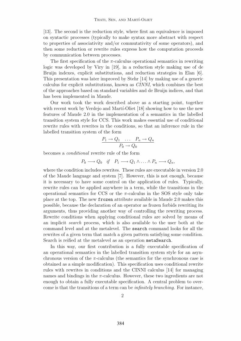
Thati, Sen, and Martı-Oliet

[13]. The second is the reduction style, where first an equivalence is imposedon syntactic processes (typically to make syntax more abstract with respectto properties of associativity and/or commutativity of some operators), andthen some reduction or rewrite rules express how the computation proceedsby communication between processes.

The first specification of the π-calculus operational semantics in rewritinglogic was developed by Viry in [19], in a reduction style making use of deBruijn indexes, explicit substitutions, and reduction strategies in Elan [6].This presentation was later improved by Stehr [14] by making use of a genericcalculus for explicit substitutions, known as CINNI, which combines the bestof the approaches based on standard variables and de Bruijn indices, and thathas been implemented in Maude.

Our work took the work described above as a starting point, togetherwith recent work by Verdejo and Martı-Oliet [18] showing how to use the newfeatures of Maude 2.0 in the implementation of a semantics in the labelledtransition system style for CCS. This work makes essential use of conditionalrewrite rules with rewrites in the conditions, so that an inference rule in thelabelled transition system of the form

P1 → Q1 . . . Pn → Qn

P0 → Q0

becomes a conditional rewrite rule of the form

P0 −→ Q0 if P1 −→ Q1 ∧ . . . ∧ Pn −→ Qn,

where the condition includes rewrites. These rules are executable in version 2.0of the Maude language and system [7]. However, this is not enough, becauseit is necessary to have some control on the application of rules. Typically,rewrite rules can be applied anywhere in a term, while the transitions in theoperational semantics for CCS or the π-calculus in the SOS style only takeplace at the top. The new frozen attribute available in Maude 2.0 makes thispossible, because the declaration of an operator as frozen forbids rewriting itsarguments, thus providing another way of controlling the rewriting process.Rewrite conditions when applying conditional rules are solved by means ofan implicit search process, which is also available to the user both at thecommand level and at the metalevel. The search command looks for all therewrites of a given term that match a given pattern satisfying some condition.Search is reified at the metalevel as an operation metaSearch.

In this way, our first contribution is a fully executable specification ofan operational semantics in the labelled transition system style for an asyn-chronous version of the π-calculus (the semantics for the synchronous case isobtained as a simple modification). This specification uses conditional rewriterules with rewrites in conditions and the CINNI calculus [14] for managingnames and bindings in the π-calculus. However, these two ingredients are notenough to obtain a fully executable specification. A central problem to over-come is that the transitions of a term can be infinitely branching. For instance,

2

384

Thati, Sen, and Martı-Oliet

the term x(y).P can evolve via an input action to one of an infinite family ofterms depending on the name received in the input at channel x. Our solutionis to define the transitions of a process relative to an execution environment.The environment is represented abstractly as a set of free (global) names thatthe environment may use while interacting with the process, and transitionsare modelled as rewrite rules over a pair consisting of a set of environmentnames together with a process.

Our next contribution is to implement the verification of the may-testingpreorder [12,3,5] between finitary (non-recursive) asynchronous π-calculus pro-cesses, using again ideas from [18] to calculate the set of all finite traces of aprocess. May testing is a specific instance of the notion of behavioral equiv-alence on π-calculus processes; in may testing, two processes are said to beequivalent if they have the same success properties in all experiments. Anexperiment consists of an observing process that runs in parallel and interactswith the process being tested, and success is defined as the observer signallinga special event. Viewing the occurrence of an event as something bad hap-pening, may testing can be used to reason about safety properties [4].

Since the definition of may testing involves a universal quantification overall observers, it is difficult to establish process equivalences directly from thedefinition. As a solution, alternate characterizations of the equivalence thatdo not resort to quantification over observers have been found. It is knownthat the trace semantics is an alternate characterization of may testing in(synchronous) π-calculus [3], while a variant of the trace semantics has beenshown to characterize may testing in an asynchronous setting [5]. Specifically,in both these cases, comparing two processes according to the may-testingpreorder amounts to comparing the set of all finite traces they exhibit. Wehave implemented for finite asynchronous processes, the comparison of tracesets proposed in [5]. We stress that our choice of specifying an asynchronousversion rather than the synchronous π-calculus, is because the characterizationof may testing for the asynchronous case is more interesting and difficult. Thesynchronous version can be specified in an executable way using similar butsimpler techniques.

Our first step in obtaining an executable specification of may testing isto obtain the set of all finite traces of a given process. This is done at theMaude metalevel by using the metaSearch operation to collect all results ofrewriting a given term. The second step is to specify a preorder relationbetween traces that characterizes may testing. We have represented the tracepreorder relation as a rewriting relation, i.e. the rules of inference that definethe trace preorder are again modeled as conditional rewrite rules. The finalstep is to check if two processes are related by the may preorder, i.e. whethera statement of the form P v Q is true or not. This step involves computingthe closure of a trace under the trace-preorder relation, again by means of themetaSearch operation. Thus, our work demonstrates the utility of the newmetalevel facilities available in Maude 2.0.

3

385

Thati, Sen, and Martı-Oliet

The structure of the paper follows the steps in the description above. Sec-tion 2 describes the syntax of the asynchronous version of the π-calculus thatwe consider, together with the corresponding CINNI operations we use. Sec-tion 3 describes the operational semantics specified by means of conditionalrewrite rules. Sections 4 and 5 define traces and the preorder on traces, re-spectively. Finally, Section 6 contains the specification of the may testing onprocesses as described above. Section 7 concludes the paper along with a briefdiscussion of future work.

Although this paper includes some information on the π-calculus and maytesting to make it as self contained as possible, we refer the reader to thepapers [5,3,11] for complete details on these subjects. In the same way, theinterested reader can find a detailed explanation about the new features ofMaude 2.0 in [7], and about their use in the implementation of operationalsemantics in the companion paper [18].

2 Asynchronous π-Calculus Syntax

The following is a brief and informal review of a version of asynchronous π-calculus that is equipped with a conditional construct for matching names. Aninfinite set of channel names is assumed, and u, v, w, x, y, z, . . . are assumed torange over it. The set of processes, ranged over by P, Q,R, is defined by thefollowing grammar:

P := xy |∑i∈I

αi.Pi | P1|P2 | (νx)P | [x = y](P1, P2) | !P

where α can be x(y) or τ .

The output term xy denotes an asynchronous message with target x andcontent y. The summation

∑i∈I αi.Pi non-deterministically chooses an αi,

and if αi = τ it evolves internally to Pi, and if αi = x(y) it receives anarbitrary name z at channel x and then behaves like Pz/y. The processPz/y is the result of the substitution of free occurrences of y in P by z,with the usual renaming of bound names to avoid accidental captures (thussubstitution is defined only modulo α-equivalence). The argument y in x(y).Pbinds all free occurrences of y in P . The composition P1|P2 consists of P1 andP2 acting in parallel. The components can act independently, and also interactwith each other. The restriction (νx)P behaves like P except that it can notexchange messages targeted to x, with its environment. The restriction bindsfree occurrences of x in P . The conditional [x = y](P1, P2) behaves like P1

if x and y are identical, and like P2 otherwise. The replication !P providesan infinite number of copies of P . The functions for free names fn(.), boundnames bn(.) and names n(.), of a process, are defined as expected.

In the Maude specification for the π-calculus syntax that follows, the sortChan is used to represent channel names and each of the non-constant syn-tax constructors is declared as frozen, so that the corresponding arguments

4

386

Thati, Sen, and Martı-Oliet

cannot be rewritten by rules; this will be justified at the end of Section 3.

sort Chan .sorts Guard GuardedTrm SumTrm Trm .subsort GuardedTrm < SumTrm .subsort SumTrm < Trm .

op _(_) : Chan Qid -> Guard .op tau : -> Guard .op nil : -> Trm .op _<_> : Chan Chan -> Trm [frozen] .op _._ : Guard Trm -> GuardedTrm [frozen] .op _+_ : SumTrm SumTrm -> SumTrm [frozen assoc comm] .op _|_ : Trm Trm -> Trm [frozen assoc comm] .op new[_]_ : Qid Trm -> Trm [frozen] .op if_=_then_else_fi : Chan Chan Trm Trm -> Trm [frozen] .op !_ : Trm -> Trm [frozen] .

Note that the syntactic form∑

i∈I αi.Pi has been split into three cases:

(i) nil represents the case where I = ∅,(ii) a term of sort GuardedTrm represents the case where I = 1, and

(iii) a term of sort SumTrm represents the case where I = [1..n] for n > 1. Sincethe constructor + is associative and the sort GuardedTrm is a subsort ofSumTrm, we can represent a finite sum

∑i∈I αi.Pi as (. . . (α1.P1 +α2.P2)+

· · ·αn.Pn).

To represent substitution on π-calculus processes (and traces, see Sec-tion 4) at the language level we use CINNI as a calculus for explicit substitu-tions [14]. This gives a first-order representation of terms with bindings andcapture-free substitutions, instead of going to the metalevel to handle namesand bindings. The main idea in such a representation is to keep the boundnames inside the binders as it is, but to replace its use by the name followedby an index which is a count of the number of binders with the same name itjumps before it reaches the place of use. Following this idea, we define termsof sort Chan as indexed names as follows.

sort Chan .op __ : Qid Nat -> Chan [prec 1] .

We introduce a sort of substitutions Subst together with the followingoperations:

op [_:=_] : Qid Chan -> Subst .op [shiftup_] : Qid -> Subst .op [shiftdown_] : Qid -> Subst .op [lift__] : Qid Subst -> Subst .

The first two substitutions are basic substitutions representing simple andshiftup substitutions; the third substitution is a special case of simple substi-tution; the last one represents complex substitution where a substitution canbe lifted using the operator lift. The intuitive meaning of these operations

5

387

Thati, Sen, and Martı-Oliet

[a := x] [shiftup a] [shiftdown a] [lift a S]

a0 7→ x a0 7→ a1 a0 7→ a0 a0 7→ [shiftup a] (S a0)a1 7→ a0 a1 7→ a2 a1 7→ a0 a1 7→ [shiftup a] (S a1)

· · · · · · · · · · · ·an+1 7→ an an 7→ an+1 an+1 7→ an an 7→ [shiftup a] (S an)bm 7→ bm bm 7→ bm bm 7→ bm bm 7→ [shiftup a] (S bm)

Table 1The CINNI operations.

is described in Table 1 (see [14] for more details). Using these, explicit sub-stitutions for π-calculus processes are defined equationally. Some interestingequations are the following:

eq S (P + Q) = (S P) + (S Q) .eq S (CX(Y) . P ) = (S CX)(Y) . ([lift Y S] P) .eq S (new [X] P) = new [X] ([lift X S] P) .

3 Operational Semantics

A labelled transition system (see Table 2) is used to give an operational se-mantics for the calculus as in [5]. The transition system is defined moduloα-equivalence on processes in that α-equivalent processes have the same tran-sitions. The rules COM, CLOSE, and PAR have symmetric versions that arenot shown in the table.

Transition labels, which are also called actions, can be of five forms: τ (asilent action), xy (free output of a message with target x and content y), x(y)(bound output), xy (free input of a message), and x(y) (bound input). Thefunctions fn(.), bn(.) and n(.) are defined on actions as expected. The set ofall visible (non-τ) actions is denoted by L, and α is assumed to range overL. As a uniform notation for free and bound actions the following notationalconvention is adopted: (∅)xy = xy, (y)xy = x(y), and similarly for inputactions. The variable z is assumed to range over ∅, z. The term (νz)P is(νz)P if z = z, and P otherwise.

We define the sort Action and the corresponding operations as follows:

sorts Action ActionType .ops i o : -> ActionType .op f : ActionType Chan Chan -> Action .op b : ActionType Chan Qid -> Action .op tauAct : -> Action .

The operators f and b are used to construct free and bound actions re-spectively. Name substitution on actions is defined equationally as expected.

The inference rules in Table 2 are modelled as conditional rewrite rules

6

388

Thati, Sen, and Martı-Oliet

INP:∑

i∈I αi.Pixjz−→ Pjz/y j ∈ I, αj = xj(y)

TAU:∑

i∈I αi.Piτ−→ Pj j ∈ I, αj = τ

OUT: xyxy−→ 0

BINP:P

xy−→ P ′

Px(y)−→ P ′

y /∈ fn(P )

PAR:P1

α−→ P ′1

P1|P2α−→ P ′

1|P2

bn(α) ∩ fn(P2) = ∅ COM:P1

xy−→ P ′1 P2

xy−→ P ′2

P1|P2τ−→ P ′

1|P ′2

RES:P

α−→ P ′

(νy)Pα−→ (νy)P ′

y /∈ n(α) OPEN:P

xy−→ P ′

(νy)Px(y)−→ P ′

x 6= y

CLOSE:P1

x(y)−→ P ′1 P2

xy−→ P ′2

P1|P2τ−→ (νy)(P ′

1|P ′2)

y /∈ fn(P2) REP:P |!P α−→ P ′

!Pα−→ P ′

IF:P

α−→ P ′

[x = x](P, Q)α−→ P ′

ELSE:Q

α−→ Q′

[x = y](P, Q)α−→ Q′

x 6= y

Table 2A labelled transition system for asynchronous π-calculus.

with the premises as conditions of the rule. 1 Since rewrites do not have labelsunlike the labelled transitions, we make the label a part of the resulting term;thus rewrites corresponding to transitions in the operational semantics are ofthe form P ⇒ αQ.

Because of the INP and OPEN rules, the transitions of a term can beinfinitely branching. Specifically, in case of the INP rule there is one branchfor every possible name that can be received in the input. In case of the OPENrule, there is one branch for every name that is chosen to denote the privatechannel that is being emitted (note that the transition rules are defined onlymodulo α-equivalence). To overcome this problem, we define transitions overpairs of the form [CS] P, where CS is a set of channel names containing all thenames that the environment with which the process interacts, knows about.The set CS expands during bound input and output interactions when privatenames are exchanged between the process and its environment.

The infinite branching due to the INP rule is avoided by allowing only thenames in the environment set CS to be received in free inputs. Since CS isassumed to contain all the free names in the environment, an input argumentthat is not in CS would be a private name of the environment. Now, sincethe identifier chosen to denote the fresh name is irrelevant, all bound input

1 The symmetric versions missing in the table need not be implemented because the processconstructors + and | have been declared as commutative.

7

389

Thati, Sen, and Martı-Oliet

transitions can be identified to a single input. With these simplifications,the number of input transitions of a term become finite. Similarly, in theOPEN rule, since the identifier chosen to denote the private name emitted isirrelevant, instances of the rule that differ only in the chosen name are notdistinguished.

We discuss in detail the implementation of only a few of the inference rules;the reader is referred to the appendix for a complete list of all the rewrite rulesfor Table 2.

sorts EnvTrm TraceTrm .subsort EnvTrm < TraceTrm .op [_]_ : Chanset Trm -> EnvTrm [frozen] .op __ : Action TraceTrm -> TraceTrm [frozen] .

Note that the two operators are also declared above with the frozen at-tribute, forbidding in this way rewriting of their arguments, as justified at theend of this section.

The following non-conditional rule is for free inputs.

rl [Inp] : [CY CS] ((CX(X) . P) + SUM) =>f(i,CX,CY) ([CY CS] ([X := CY] P)) .

The next rule we consider is the one for bound inputs. Since the identifierchosen to denote the bound argument is irrelevant, we use the constant ’U

for all bound inputs, and thus ’U0 denotes the fresh channel received. Notethat in contrast to the BINP rule of Table 2, we do not check if ’U0 is in thefree names of the process performing the input, and instead we shift up thechannel indices appropriately, in both the set of environment names CS andthe process P in the righthand side and condition of the rule. This is justifiedbecause the transition target is within the scope of the bound name in theinput action. Note also that the channel CX in the action is not shifted downbecause it is out of the scope of the bound argument. The set of environmentnames is expanded by adding the received channel ’U0 to it. Finally, weuse a special constant flag of sort Chan, to ensure termination. We add aninstance of flag to the environment set of the rewrite in condition, so thatthe BINP rule is not fired again while evaluating the condition. Without thischeck, we will have a non-terminating execution in which the BINP rule isrepeatedly fired.

crl [BInp] : [CS] P => b(i,CX,’U) [’U0 [shiftup ’U] CS] P1if (not flag in CS) /\

CS1 := flag ’U0 [shiftup ’U] CS /\[CS1] [shiftup ’U] P => f(i,CX,’U0) [CS1] P1 .

The following rule treats the case of bound outputs.

crl [Open] : [CS] (new [X] P) => [shiftdown X] b(o,CY,X) [X0 CS1] P1if CS1 := [shiftup X] CS /\

[CS1] P => f(o,CY,X0) [CS1] P1 /\ X0 =/= CY .

Like in the case of bound inputs, we identify all bound outputs to a single

8

390

Thati, Sen, and Martı-Oliet

instance in which the identifier X that appears in the restriction is chosen asthe bound argument name. Note that in both the righthand side of the ruleand in the condition, the indices of the channels in CS are shifted up, becausethey are effectively moved across the restriction. Similarly, the channel indicesin the action in the righthand side of the rule are shifted down since the actionis now moved out of the restriction. Note also that the exported name is addedto the set of environment names, because the environment that receives thisexported name can use it in subsequent interactions.

The PAR inference rule is implemented by two rewrite rules, one for thecase where the performed action is free, and the other where the action isbound. The rewrite rule for the latter case is discussed next, while the one forthe former case is simpler and appears in the appendix.

var IO : ActionTypecrl [Par] : [CS] (P | Q) =>

b(IO,CX,Y) [Y0 ([shiftup Y] CS)] (P1 | [shiftup Y] Q)if [CS] P => b(IO,CX,Y) ([CS1] P1) .

Note that the side condition of the PAR rule in Table 2, which avoidsconfusion of the emitted bound name with free names in Q, is achieved byshifting up channel indices in Q. This is justified because the righthand side ofthe rule is under the scope of the bound output action. Similarly, the channelindices in the environment are also shifted up. Further, the set of environmentnames is expanded by adding the exported channel Y0.

Finally, we consider the rewrite rule for CLOSE. The process P emits abound name Y, which is received by process Q. Since the scope of Y after thetransition includes Q, the rewrite involving Q in the second condition of therule is carried out within the scope of the bound name that is emitted. Thisis achieved by adding the channel Y0 to the set of environment names andshifting up the channel indices in both CS and Q in the rewrite. Note thatsince the private name being exchanged is not emitted to the environment,we neither expand the set CS in the righthand side of the rule nor shift up thechannel indices in it.

crl [Close] : [CS] (P | Q) => tauAct [CS] new [Y] (P1 | Q1)if [CS] P => b(o,CX,Y) [CS1] P1 /\

[Y0 [shiftup Y] CS] [shiftup Y] Q =>f(i,CX,Y0) [CS2] Q1 .

We conclude this section with the following note. The operator isdeclared frozen because further rewrites of the process term encapsulatedin a term of sort TraceTrm are useless. This is because all the conditions ofthe transition rules only involve one step rewrites (the righthand side of theserewrites can only match a term of sort TraceTrm with a single action prefix).Further note that, to prevent rewrites of a term to a non well-formed term, allthe constructors for π-calculus terms (Section 2) have been declared frozen;in the absence of this declaration we would have for instance rewrites of theform P | Q => A.P1 | Q to a non well-formed term.

9

391

Thati, Sen, and Martı-Oliet

4 Trace Semantics

The set L∗ is the set of traces. The functions fn(.), bn(.) and n(.) are extendedto L∗ in the obvious way. The relation of α-equivalence on traces is definedas expected, and α-equivalent traces are not distinguished. The relation =⇒denotes the reflexive transitive closure of

τ−→, andβ

=⇒ denotes =⇒ β−→=⇒.

For s = l.s′, we inductively define Ps

=⇒ P ′ as Pl

=⇒ s′=⇒ P ′. We use P

s=⇒

as an abbreviation for Ps

=⇒ P ′ for some P ′. The set of traces that a processexhibits is then [|P |] = s | P

s=⇒.

In the implementation, we introduce a sort Trace as supersort of Actionto specify traces.

subsort Action < Trace .op epsilon : -> Trace .op _._ : Trace Trace -> Trace [assoc id: epsilon] .op [_] : Trace -> TTrace .

We define the operator [ ] to represent a complete trace. The motivationfor doing so is to restrict the equations and rewrite rules defined over traces tooperate only on a complete trace instead of a part of it. The following equationdefines α-equivalence on traces. Note that in a trace TR1.b(IO,CX,Y).TR2 theaction b(IO,CX,Y) binds the identifier Y in TR2.

ceq [TR1 . b(IO,CX,Y) . TR2] =[TR1 . b(IO,CX,’U) . [Y := ’U0] [shiftup ’U] TR2]

if Y =/= ’U .

Because the operator op : Action TraceTrm -> TraceTrm is declaredas frozen, a term of sort EnvTrm can rewrite only once, and so we cannot ob-tain the set of finite traces of a process by simply rewriting it multiple times inall possible ways. The problem is solved as in [18], by specifying the trace se-mantics using rules that generate the transitive closure of one step transitionsas follows:

sort TTrm .op [_] : EnvTrm -> TTrm [frozen] .var TT : TraceTrm .

crl [reflx] : [ P ] => A Q if P => A Q .crl [trans] : [ P ] => A TT

if P => A Q /\ [ Q ] => TT /\ [ Q ] =/= TT .

We use the operator [ ] to prevent infinite loops while evaluating theconditions of the rules above. If this operator were not used, then the lefthandside of the rewrite in the condition would match the lefthand side of the ruleitself, and so the rule itself could be used in order to solve its condition. Thisoperator is also declared as frozen to prevent useless rewrites inside [ ].

We can now use the search command of Maude 2.0 to find all possibletraces of a process. The traces appear as prefix of the one-step successorsof a TTrm of the form [[CS] P]. For instance, the set of all traces exhibited

10

392

Thati, Sen, and Martı-Oliet

by [mt] new [’y] (’x0 < ’y0 > | ’x0(’u) . nil) (where mt denotes theempty channel set), can be obtained by using the following search command.

Maude> search [ [mt] new [’y] (’x0 < ’y0 > | ’x0(’u) . nil) ] =>!X:TraceTrm .search in APITRACESET : [[mt]new[’y](’x0 < ’y0 > | ’x0(’u) . nil)] =>!X:TraceTrm .

Solution 1 (state 1)states: 7 rewrites: 17344 in 110ms cpu (150ms real) (157672 rewrites/second)X:TraceTrm --> b(i, ’x0, ’u)[’u0]new[’y](nil | ’x0 < ’y0 >)

Solution 2 (state 2)states: 7 rewrites: 17344 in 110ms cpu (170ms real) (157672 rewrites/second)X:TraceTrm --> tauAct[mt]new[’y](nil | nil)

Solution 3 (state 3)states: 7 rewrites: 17344 in 110ms cpu (170ms real) (157672 rewrites/second)X:TraceTrm --> b(o, ’x0, ’y)[’y0]nil | ’x0(’u) . nil

Solution 4 (state 4)states: 7 rewrites: 17344 in 110ms cpu (170ms real) (157672 rewrites/second)X:TraceTrm --> b(i, ’x0, ’u)b(o, ’x0, ’y)[’y0 ’u0]nil | nil

Solution 5 (state 5)states: 7 rewrites: 17344 in 110ms cpu (170ms real) (157672 rewrites/second)X:TraceTrm --> b(o, ’x0, ’y)b(i, ’x0, ’u)[’y0 ’u0]nil | nil

Solution 6 (state 6)states: 7 rewrites: 17344 in 110ms cpu (170ms real) (157672 rewrites/second)X:TraceTrm --> b(o, ’x0, ’y)f(i, ’x0, ’y0)[’y0]nil | nil

No more solutions.states: 7 rewrites: 17344 in 110ms cpu (170ms real) (157672 rewrites/second)

The command returns all TraceTrms that can be reached from the givenTTrm, and that are terminating (the ‘!’ in =>! specifies that the target shouldbe terminating). The required set of traces can be obtained by simply extract-ing from each solution a1...anTT the sequence a1...an and removingall tauActs in it. Thus, we have obtained an executable specification of thetrace semantics of asynchronous π-calculus.

5 A Trace Based Characterization of May Testing

The may-testing framework [12] is instantiated on asynchronous π-calculus asfollows. Observers are processes that can emit a special message µµ. We say

that an observer O accepts a trace s if Os.µµ=⇒, where s is the trace obtained by

complementing the actions in s, i.e. converting input actions to output actionsand vice versa. The may preorder v over processes is defined as: P v Q if for

every observer O, P |O µµ=⇒ implies Q|O µµ

=⇒. We say that P and Q are may-

11

393

Thati, Sen, and Martı-Oliet

(Drop) s1.(y)s2 ≺ s1.(y)xy.s2 if (y)s2 6= ⊥(Delay) s1.(y)(α.xy.s2) ≺ s1.(y)xy.α.s2 if (y)(α.xy.s2) 6= ⊥

(Annihilate) s1.(y)s2 ≺ s1.(y)xy.xy.s2 if (y)s2 6= ⊥Table 3

A preorder relation on traces.

equivalent, i.e. P = Q, if P v Q and Q v P . The universal quantificationon contexts in this definition makes it very hard to prove equalities directlyfrom the definition, and makes mechanical checking impossible. To circumventthis problem, a trace based alternate characterization of the may equivalenceis proposed in [5]. We now summarize this characterization and discuss ourimplementation of it.

The preorder ¹ on traces is defined as the reflexive transitive closure ofthe laws shown in Table 3, where the notation (y)· is extended to traces asfollows.

(y)s =

s if y = ∅ or b 6∈ fn(s)

s1.x(y).s2 if y = y and there are s1, s2, x such that

s = s1.xy.s2 and y 6∈ n(s1) ∪ x⊥ otherwise

For sets of traces R and S, we define R - S, if for every s ∈ S there isan r ∈ R such that r ¹ s. The may preorder is then characterized in [5] as:P v Q if and only if [|Q|] - [|P |].

The main intuition behind the preorder ¹ is that if an observer acceptsa trace s, then it also accepts any trace r ¹ s. The first two laws state thatan observer cannot force inputs on the process being tested. Since outputsare asynchronous, the actions following an output in a trace exhibited by theobserver need not causally depend on the output. Hence the observer’s outputcan be delayed until a causally dependent action, or dropped if there are nosuch actions. The annihilation law states that an observer can consume itsown outputs unless there are subsequent actions that depend on the output.The reader is referred to [5] for further details on this characterization.

We encode the trace preorder as rewrite rules on terms of the sort TTraceof complete traces; specifically, the relation r ≺ s if cond, is encoded as s

=> r if cond. The reason for this form of representation will be justifiedin Section 6. The function (y)· on traces is defined equationally by theoperation bind. The constant bot of sort Trace is used by the bind operationto signal error.

op bind : Qid Trace -> Trace .op bot : -> Trace .var TR : Trace . var IO : ActionType.

12

394

Thati, Sen, and Martı-Oliet

ceq TR . bot = bot if t =/= epsilon .ceq bot . TR = bot if t =/= epsilon .

eq bind(X , epsilon) = epsilon .

eq bind(X , f(i,CX,CY) . TR ) = if CX =/= X0 thenif CY == X0 then ([shiftdown X] b(i, CX , X)) . TR

else ([shiftdown X] f(i, CX , CY)) . bind(X , TR) fielse bot fi .

eq bind(X , b(IO,CX,Y) . TR) = if CX =/= X0 thenif X =/= Y then ([shiftdown X] b(i, CX , Y)) . bind(X , TR)

else ([shiftdown X] b(IO, CX , Y)) . bind(X , swap(X,TR)) fielse bot fi .

The equation for the case where the second argument to bind begins witha free output is not shown as it is similar. Note that the channel indicesin actions until the first occurrence of X0 as the argument of a free inputare shifted down as these move out of the scope of the binder X. Further,when a bound action with X as the bound argument is encountered, the swap

operation is applied to the remaining suffix of the trace. The swap operationsimply changes the channel indices in the suffix so that the binding relationis unchanged even as the binder X is moved across the bound action. This isaccomplished by simultaneously substituting X0 with X1, and X1 withX0. Finally, note that when X0 is encountered as the argument of a freeinput, the input is converted to a bound input. If X0 is first encountered atany other place, an error is signalled by returning the constant bot.

The encoding of the preorder relation on traces is now straightforward.

crl [Drop] : [ TR1 . b(i,CX,Y) . TR2 ] => [ TR1 . bind(Y , TR2) ]if bind(Y , TR2) =/= bot .

rl [Delay] : [ ( TR1 . f(i,CX,CY) . b(IO,CU,V) . TR2 ) ] =>[ ( TR1 . b(IO,CU,V) . ([shiftup V] f(i, CX , CY)) . TR2 ) ] .

crl [Delay] : [ ( TR1 . b(i,CX,Y) . f(IO,CU,CV) . TR2 ) ] =>[ ( TR1 . bind(Y , f(IO,CU,CV) . f(i,CX,Y0) . TR2) ) ]

if bind(Y , f(IO,CU,CV) . f(i,CX,Y0) . TR2) =/= bot .

crl [Annihilate] : [ ( TR1 . b(i,CX,Y) . f(o,CX,Y0) . TR2 ) ] =>[ TR1 . bind(Y , TR2) ]

if bind(Y , TR2) =/= bot .

Note that in the first Delay rule, the channel indices of the free inputaction are shifted up when it is delayed across a bound action, since it getsinto the scope of the bound argument. Similarly, in the second Delay rule,when the bound input action is delayed across a free input/output action,the channel indices of the free action are shifted down by the bind operation.The other two subcases of the Delay rule, namely, where a free input is tobe delayed across a free input or output, and where a bound input is to bedelayed across a bound input or output, are not shown as they are similar.

13

395

Thati, Sen, and Martı-Oliet

Similarly, for Annihilate, the case where a free input is to be annihilatedwith a free output is not shown.

6 Verifying the May Preorder between Finite Processes

We now describe our implementation of verification of the may preorder be-tween finite processes, i.e. processes without replication, by exploiting thetrace-based characterization of may testing discussed in Section 5. The finite-ness of a process P only implies that the length of traces in [|P |] is bounded,but the number of traces in [|P |] can be infinite (even modulo α-equivalence)because the INP rule is infinitely branching. To avoid the problem of havingto compare infinite sets, we observe that

[|Q|] - [|P |] if and only if [|Q|]fn(P,Q) - [|P |]fn(P,Q),

where for a set of traces S and a set of names ρ we define Sρ = s ∈ S |fn(s) ⊆ ρ. Now, since the traces in [|P |] and [|Q|] are finite in length, itfollows that the sets of traces [|P |]fn(P,Q) and [|Q|]fn(P,Q) are finite modulo α-equivalence. In fact, the set of traces generated for [[fn(P,Q)] P] by ourimplementation described in Section 3, contains exactly one representativefrom each α-equivalence class of [|P |]fn(P,Q).

Given processes P and Q, we generate the set of all traces (modulo α-equivalence) of [[fn(P,Q)] P] and [[fn(P,Q)] Q] using the metalevel fa-cilities of Maude 2.0. As mentioned in Section 4, these terms, which areof sort TTrm, can be rewritten only once. The term of sort TraceTrm ob-tained by rewriting contains a finite trace as a prefix. To create the set of alltraces, we compute all possible one-step rewrites. This computation is done atthe metalevel by the function TTrmtoNormalTraceSet that uses two auxiliaryfunctions TTrmtoTraceSet and TraceSettoNormalTraceSet.

op TTrmtoTraceSet : Term -> TermSet .op TraceSettoNormalTraceSet : TermSet -> TermSet .op TTrmtoNormalTraceSet : Term -> TermSet .

eq TTrmtoNormalTraceSet(T) = TraceSettoNormalTraceSet(TTrmtoTraceSet(T)) .

The function TTrmTraceSet uses the function allOneStepAux(T,N) thatreturns the set of all one-step rewrites (according to the rules in Sections 3and 4, which are defined in modules named APISEMANTICS and APITRACE, seeFigure A.1 in appendix) of the term T which is the metarepresentation of aterm of sort TTrm, skipping the first N solutions. In the following equations,the operator u stands for set union.

Notice the use of the operation metaSearch, which receives as argumentsthe metarepresented module to work in, the starting term for search, thepattern to search for, a side condition (empty in this case), the kind of search(which may be ’* for zero or more rewrites, ’+ for one or more rewrites, and’! for only matching normal forms), the depth of search, and the requiredsolution number. It returns the term matching the pattern, its type, and

14

396

Thati, Sen, and Martı-Oliet

the substitution produced by the match; to keep only the term, we use theprojection getTerm.

op APITRACE-MOD : -> Module .eq APITRACE-MOD = [’APITRACE] .var N : MachineInt . vars T X : Term .

op allOneStepAux : Term MachineInt Term -> TermSet .op TraceTermToTrace : Term -> Term .

eq TTrmtoTraceSet(T) = allOneStepAux(T,0,’X:TraceTrm) .eq allOneStepAux(T,N,X) =

if metaSearch(APITRACE-MOD,T,X,nil,’+,1,N) == failurethen ’epsilon.Traceelse TraceTermToTrace(getTerm(metaSearch(APITRACE-MOD,T,X,nil,’+,1,N)))

u allOneStepAux(T,N + 1,X) fi .

The function TraceTrmToTrace (whose equations are not shown), usedin allOneStepAux, extracts the trace a1.a2...an out of a metarepresenta-tion of a term of sort TraceTrm of the form a1a2...anTT. The functionTraceSettoNormalTraceSet uses the metalevel operation metaReduce to con-vert each trace in a trace set to its α-normal form. The operation metaReduce

takes as arguments a metarepresented module and a metarepresented termin that module, and returns the metarepresentation of the fully reduced formof the given term using the equations in the given module, together with itscorresponding sort or kind. Again, the projection getTerm leaves only theresulting term.

eq TraceSettoNormalTraceSet(mt) = mt .eq TraceSettoNormalTraceSet(T u TS) =

getTerm(metaReduce(TRACE-MOD,’‘[_‘] [ T ]))u TraceSettoNormalTraceSet(TS) .

We implement the relation - on sets defined in Section 5 as the predicate<<. We check if P v Q by computing this predicate on the metarepresentedtrace sets [|P |]fn(P,Q) and [|Q|]fn(P,Q) as follows. For each (metarepresented)trace T in [|P |]fn(P,Q), we compute the reflexive transitive closure of T withrespect to the laws shown in Table 3. The laws are implemented as rewriterules in the module TRACE-PREORDER. We then use the fact that [|Q|]fn(P,Q) -[|P |]fn(P,Q) if and only if for every trace T in [|P |]fn(P,Q) the closure of T and[|Q|]fn(P,Q) have a common element.

op TRACE-PREORDER-MOD : -> Module .eq TRACE-PREORDER-MOD = [’TRACE-PREORDER] .var N : MachineInt . vars T T1 T2 X : Term .var TS TS1 TS2 : TermSet .

op _<<_ : TermSet TermSet -> Bool .op _<<<_ : TermSet Term -> Bool .op TTraceClosure : Term -> TermSet .op TTraceClosureAux : Term Term MachineInt -> TermSet .op _maypre_ : Term Term -> Bool .

15

397

Thati, Sen, and Martı-Oliet

eq TS2 << mt = true .eq TS2 << (T1 u TS1) = TS2 <<< T1 and TS2 << TS1 .eq TS2 <<< T1 = not disjoint?(TS2 , TTraceClosure(T1)) .eq T1 maypre T2 = TTrmtoNormalTraceSet(T2) << TTrmtoNormalTraceSet(T1) .

The computation of the closure of T is done by the function TTraceClosure.It uses TTraceClosureAux to compute all possible (multi-step) rewrites of theterm T using the rules defined in the module TRACE-PREORDER, again by meansof the metalevel operation metaSearch.

eq TTraceClosure(T) = TTraceClosureAux(T,’TT:TTrace,0) .eq TTraceClosureAux(T,X,N) =

if metaSearch(TRACE-PREORDER-MOD,T,X,nil,’*,maxMachineInt,N) == failurethen mtelse getTerm(metaSearch(TRACE-PREORDER-MOD,T,X,nil,’*,maxMachineInt,N))

u TTraceClosureAux(T,X,N + 1) fi .

This computation is terminating as the number of traces to which a tracecan rewrite using the trace preorder laws is finite modulo α-equivalence. Thisfollows from the fact that the length of a trace is non-increasing across rewrites,and the free names in the target of a rewrite are also free names in the source.Since the closure of a trace is finite, metaSearch can be used to enumerate allthe traces in the closure. Note that although the closure of a trace is finite, itis possible to have an infinite rewrite that loops within a subset of the closure.Further, since T is a metarepresentation of a trace, metaSearch can be applieddirectly to T inside the function TTraceClosureAux(T,X,N).

We end this section with a small example, which checks for the may-testingpreorder between the processes P = a(u).b(v).(νw)(wv|au)+b(u).a(v).(bu|bw)and Q = b(u).(bu|bw). We define constants TP and TQ of sort TTrm, along withthe following equations:

eq TP = [[’a0 ’b0 ’w0]’a0(’u) . ’b0(’v) . new[’w](’w0 < ’v0 > | ’a0 < ’u0 >)

+ ’b0(’u) . ’a0(’v) . (’b0 < ’u0 > | ’b0 < ’w0 >)]

eq TQ = [[’a0 ’b0 ’w0]’b0(’u) . (’b0 < ’u0 > | ’b0 < ’w0 >)]

The metarepresentation of these TTrms can now be obtained by using’TP.TTrm and ’TQ.TTrm, and we can then check for the may-testing preorderbetween the given processes as follows:

Maude> red ’TP.TTrm maypre ’TQ.TTrm .reduce in APITRACESET : ’TP.TTrm maypre ’TQ.TTrm .rewrites: 791690 in 2140ms cpu (2160ms real) (361422 rewrites/second)result Bool: trueMaude> red ’TQ.TTrm maypre ’TP.TTrm .reduce in APITRACESET : ’TQ.TTrm maypre ’TP.TTrm .rewrites: 664833 in 1620ms cpu (1640ms real) (410390 rewrites/second)result Bool: false

Thus, we have P v Q, but Q /v P . The reader can check that indeed,[|Q|]fn(P,Q) - [|P |]fn(P,Q), but [|P |]fn(P,Q) /- [|Q|]fn(P,Q).

16

398

Thati, Sen, and Martı-Oliet

7 Conclusions and Future Work

In this paper, we have described an executable specification in Maude of theoperational semantics of an asynchronous version of the π-calculus using con-ditional rewrite rules with rewrites in the conditions as proposed by Verdejoand Martı-Oliet in [18], and the CINNI calculus proposed by Stehr in [14]for managing names and their binding. In addition, we also implementedthe may-testing preorder for π-calculus processes using the Maude metalevel,where we use the metaSearch operation to calculate the set of all traces for aprocess and then compare two sets of traces according to a preorder relationbetween traces. As emphasized throughout the paper, the new features intro-duced in Maude 2.0 have been essential for the development of this executablespecification, including rewrites in conditions, the frozen attribute, and themetaSearch operation.

An interesting direction of further work is to extend our implementationto the various typed variants of π-calculus. Two specific typed asynchronousπ-calculi for which the work is under way are the local π-calculus (Lπ) [10]and the Actor model [1,15]. Both of these formal systems have been usedextensively in formal specification and analysis of concurrent object-orientedlanguages [2,8], and open distributed and mobile systems [9]. The alternatecharacterization of may testing for both of these typed calculi was recentlypublished [16,17]. We are extending the work presented here to account forthe type systems for these calculi, and modifications to the trace based char-acterization of may testing. We are also looking for interesting concrete appli-cations to which this can be applied; such experiments may require extendingour implementation to extensions of π-calculus with higher level constructs,although these may just be syntactic sugar.

Acknowledgements

This research has been supported in part by the Defense Advanced ResearchProjects Agency (contract numbers F30602-00-2-0586 and F33615-01-C-1907),the ONR MURI Project A Logical Framework for Adaptive System Inter-operability, and the Spanish CICYT project Desarrollo Formal de SistemasBasados en Agentes Moviles (TIC2000–0701–C02–01). This work was donewhile the last author was visiting the Department of Computer Science inthe University of Illinois at Urbana-Champaign, for whose hospitality he isvery grateful. We would like to thank Jose Meseguer for encouraging us toput together several complementary lines of work in order to get the resultsdescribed in this paper.

References

[1] G. Agha. Actors: A Model of Concurrent Computation in Distributed Systems.MIT Press, 1986.

17

399

Thati, Sen, and Martı-Oliet

[2] G. Agha. Concurrent object-oriented programming. Communications of theACM, 33(9):125–141, September 1990.

[3] M. Boreale and R. De Nicola. Testing equivalence for mobile processes.Information and Computation, 120:279–303, 1995.

[4] M. Boreale, R. De Nicola, and R. Pugliese. Proof techniques for cryptographicprocesses. In Proceedings 14th IEEE Symposium on Logic in Computer Science,LICS’99, Trento, Italy, July 2–5, 1999, pages 157–166. IEEE Computer SocietyPress, 1999.

[5] M. Boreale, R. De Nicola, and R. Pugliese. Trace and testing equivalence onasynchronous processes. Information and Computation, 172(2):139–164, 2002.

[6] P. Borovansky, C. Kirchner, H. Kirchner, P.-E. Moreau, and M. Vittek.ELAN: A logical framework based on computational systems. In J. Meseguer,editor, Proceedings First International Workshop on Rewriting Logic and itsApplications, WRLA’96, Asilomar, California, September 3–6, 1996, volume 4of Electronic Notes in Theoretical Computer Science, pages 35–50. Elsevier,1996. http://www.elsevier.nl/locate/entcs/volume4.html.

[7] M. Clavel, F. Duran, S. Eker, P. Lincoln, N. Martı-Oliet, J. Meseguer, and J.F. Quesada. Towards Maude 2.0. In K. Futatsugi, editor, Proceedings ThirdInternational Workshop on Rewriting Logic and its Applications, WRLA 2000,Kanazawa, Japan, September 18–20, 2000, volume 36 of Electronic Notes inTheoretical Computer Science, pages 297–318. Elsevier, 2000. http://www.elsevier.nl/locate/entcs/volume36.html.

[8] I. A. Mason and C. Talcott. A semantically sound actor translation. InP. Degano, R. Gorrieri, and A. Marchetti-Spaccamela, editors, Automata,Languages and Programming, 24th International Colloquium, ICALP’97,Bologna, Italy, July 7–11, 1997, Proceedings, volume 1256 of Lecture Notesin Computer Science, pages 369–378. Springer-Verlag, 1997.

[9] M. Merro, J. Kleist, and U. Nestmann. Local π-calculus at work: Mobile objectsas mobile processes. In J. van Leeuwen et al., editors, Theoretical ComputerScience: Exploring New Frontiers of Theoretical Informatics, InternationalConference IFIP TCS 2000 Sendai, Japan, August 17–19, 2000, Proceedings,volume 1872 of Lecture Notes in Computer Science, pages 390–408. Springer-Verlag, 2000.

[10] M. Merro and D. Sangiorgi. On asynchrony in name-passing calculi. InK. G. Larsen, S. Skyum, and G. Winskel, editors, Automata, Languages andProgramming, 25th International Colloquium, ICALP’98, Aalborg, Denmark,July 13–17, 1998, Proceedings, volume 1443 of Lecture Notes in ComputerScience, pages 856–867. Springer-Verlag, 1998.

[11] R. Milner, J. Parrow, and D. Walker. A calculus of mobile processes (Parts Iand II). Information and Computation, 100:1–77, 1992.

[12] R. De Nicola and M. Hennessy. Testing equivalence for processes. TheoreticalComputer Science, 34:83–133, 1984.

18

400

Thati, Sen, and Martı-Oliet

[13] G. D. Plotkin. A structural approach to operational semantics. TechnicalReport DAIMI FN-19, Computer Science Dept., Aarhus University, September1981.

[14] M.-O. Stehr. CINNI — A generic calculus of explicit substitutions and itsapplication to λ-, ς- and π-calculi. In K. Futatsugi, editor, Proceedings ThirdInternational Workshop on Rewriting Logic and its Applications, WRLA 2000,Kanazawa, Japan, September 18–20, 2000, volume 36 of Electronic Notes inTheoretical Computer Science, pages 71–92. Elsevier, 2000. http://www.elsevier.nl/locate/entcs/volume36.html.

[15] C. Talcott. An actor rewriting theory. In J. Meseguer, editor, Proceedings FirstInternational Workshop on Rewriting Logic and its Applications, WRLA’96,Asilomar, California, September 3–6, 1996, volume 4 of Electronic Notes inTheoretical Computer Science, pages 360–383. Elsevier, 1996. http://www.elsevier.nl/locate/entcs/volume4.html.

[16] P. Thati, R. Ziaei, and G. Agha. A theory of may testing for actors. In B. Jacobsand A. Rensink, editors, Proceedings IFIP TC6/WG6.1 Fifth InternationalConference on Formal Methods for Open Object-Based Distributed Systems(FMOODS 2002), March 20-22, 2002, Enschede, The Netherlands, pages 147–162. Kluwer Academic Publishers, 2002.

[17] P. Thati, R. Ziaei, and G. Agha. A theory of may testing for asynchronouscalculi with locality and no name matching. In H. Kirchner and C. Ringeissen,editors, Algebraic Methodology and Software Technology, 9th InternationalConference, AMAST 2002, Saint-Gilles-les-Bains, Reunion Island, France,September 9-13, 2002, Proceedings, volume 2422 of Lecture Notes in ComputerScience. Springer-Verlag, 2002.

[18] A. Verdejo and N. Martı-Oliet. Implementing CCS in Maude 2. In U.Montanari, editor, Proceedings Fourth International Workshop on RewritingLogic and its Applications, WRLA 2002, Pisa, Italy, September 19–21, 2002,volume 71 of Electronic Notes in Theoretical Computer Science. Elsevier, 2002.(This volume.) http://www.elsevier.nl/locate/entcs/volume71.html.

[19] P. Viry. Input/output for ELAN. In J. Meseguer, editor, Proceedings FirstInternational Workshop on Rewriting Logic and its Applications, WRLA’96,Asilomar, California, September 3–6, 1996, volume 4 of Electronic Notes inTheoretical Computer Science, pages 51–64. Elsevier, 1996. http://www.elsevier.nl/locate/entcs/volume4.html.

A Appendix

The diagram in Figure A.1 illustrates the graph of module importation in ourimplementation that closely follows the structure of the paper. The completecode is available at http://osl.cs.uiuc.edu/~ksen/api/. Here we onlyshow the module that contains the rewrite rules for the operational semantics

19

401

Thati, Sen, and Martı-Oliet

NAT QID³³³³³³

CHAN

CINNI STRING³³³³³

CHANSET

TRACEPPPPPP

APISYNTAX

TRACE-PREORDERQ

QQ

QQ

QQQ

APISEMANTICS META-LEVEL

APITRACE TERMSET©©©©

APITRACESET

Fig. A.1. The graph of module importation in the implementation.

of asynchronous π-calculus (Table 2). The function genQid used in the condi-tion of the last Res rule generates an identifier that is fresh, i.e. an identifiernot used to construct channel names in the set passed as the argument to thefunction.

mod APISEMANTICS isinc APISYNTAX .inc CHANSET .inc TRACE .sorts EnvTrm TraceTrm .subsort EnvTrm < TraceTrm .

op [_]_ : Chanset Trm -> EnvTrm [frozen] .op __ : Action TraceTrm -> TraceTrm [frozen] .op notinfn : Qid Trm -> Prop .

vars N : Nat . vars X Y Z : Qid .vars CX CY : Chan . var CS CS1 CS2 : Chanset .vars A : Action . vars P1 Q1 P Q : Trm .var SUM : SumTrm . var IO : ActionType .

eq notinfn(X,P) = not X0 in freenames(P) .

rl [Inp] : [CY CS] (CX(X) . P) =>f(i,CX,CY) ([CY CS] ([X := CY] P)) .

rl [Inp] : [CY CS] ((CX(X) . P) + SUM) =>f(i,CX,CY) ([CY CS] ([X := CY] P)) .

rl [Tau] : [CS] (tau . P) => tauAct ([CS] P) .

rl [Tau] : [CS] ((tau . P) + SUM) => tauAct ([CS] P) .

20

402

Thati, Sen, and Martı-Oliet

crl [BInp] : [CS] P => b(i,CX,’u) [’u0 [shiftup ’u] CS] P1if (not flag in CS) /\

CS1 := flag ’u0 [shiftup ’u] CS /\[CS1] [shiftup ’u] P => f(i,CX,’u0) [CS1] P1 .

rl [Out] : [CS] CX < CY > => f(o,CX,CY) ([CS] nil) .

crl [Par] : [CS] (P | Q) => f(IO,CX,CY) ([CS] (P1 | Q))if [CS] P => f(IO,CX,CY) ([CS] P1) .

crl [Par] : [CS] (P | Q) =>b(IO,CX,Y) [Y0 ([shiftup Y] CS)] (P1 | [shiftup Y] Q)

if [CS] P => b(IO,CX,Y) ([CS1] P1) .

crl [Com] : [CS] (P | Q) => tauAct ([CS] (P1 | Q1))if [CS] P => f(o,CX,CY) ([CS] P1) /\

[CY CS] Q => f(i,CX,CY) ([CY CS] Q1) .

crl [Close] : [CS] (P | Q) => tauAct [CS] new [Y] (P1 | Q1)if [CS] P => b(o,CX,Y) [CS1] P1 /\

[Y0 [shiftup Y] CS] [shiftup Y] Q =>f(i,CX,Y0) [CS2] Q1 .

crl [Res] : [CS] (new [X] P) =>[shiftdown X] f(IO,CX,CY) [CS] (new [X] P1)

if CS1 := [shiftup X] CS /\[CS1] P => f(IO,CX,CY) [CS1] P1 /\(not X0 in (CX CY)) .

crl [Res] : [CS] (new [X] P) => tauAct [CS] (new [X] P1)if [CS] P => tauAct [CS] P1 .

crl [Res] : [CS] (new [X] P) =>[shiftdown X] b(o,CX,Z) [Z0 CS] new[X]([ Y := Z0 ] P1)if Z := genQid(X0 CS freenames(P)) /\

[[shiftup X] CS] P => b(o,CX,Y) [CS1] P1 /\X0 =/= CX .

crl [Open] : [CS] (new[X] P) => [shiftdown X] b(o,CY,X) [X0 CS1] P1if CS1 := [shiftup X] CS /\

[CS1] P => f(o,CY,X0) [CS1] P1 /\ X0 =/= CY .

crl [If] : [CS1] (if CX = CX then P else Q fi) => A [CS2] P1if [CS1] P => A [CS2] P1 .

crl [Else] : [CS1] (if CX = CY then P else Q fi) => A [CS2] Q1if CX =/= CY /\ [CS1] Q => A [CS2] Q1 .

crl [Rep] : [CS1] (! P) => A [CS2] P1if [CS1] (P | (! P)) => A [CS2] P1 .

endm

21

403

13Thin Middleware for

Ubiquitous Computing

Koushik SenGul Agha

13.1 INTRODUCTION

As Donald Norman put it in his popular book Invisible Computers [12], “a goodtechnology is a disappearing technology.” A good technology seamlessly permeatesinto our lives in such a way that we use it without noticing its presence. It is invisibleuntil it is not available. Ever since the invention of microprocessors, many computerresearchers have strived to make computer technology a “good” technology.

Advances in chip fabrication technology have reached a point where we can physi-cally make computing devices disappear. Bulkier machines have given way to smalleryet more powerful personal computers. It has become possible to implant a completepackage of a microprocessor with wireless communication, storage, and a sensor ona cubic millimeter silicon die [8]. Specialized printers print out computer chips ona piece of plastic paper [6]. Computer chips are woven into on a piece of fabric [9].“Smart labels” (a.k.a passive RFID tags) [7] will soon be attached to every productin the market.

The growth of devices with embedded computers will provide task-oriented, simpleservices which are highly optimized for their operating environment. More useroriented, human friendly services may be created by networking the embedded nodes,and coordinating their software services.

Composing existing component services to create higher-level services has beenpromoted by CORBA, DCOM, Jini, and similar middleware platforms. However,these middleware services were designed without paying much attention to resourcemanagement issues pertinent to embedded nodes: the middlewares tend to have large

201

404

footprints that do not fit into the typically small memories of tiny embedded com-puters. Thus there is a need for a middleware which allows components to be gluedtogether without a large overhead.

Embedded nodes are autonomous and self contained. They have their own stateand a single thread of control, and a well defined interface for interaction. Interactionbetween nodes is asynchronous in nature. The operating environment for these de-vices may be unreliable. For these reasons, the interaction between different devicesmust be arms-length – the failure of one device should not affect another. For exam-ple, consider an intelligent home where the clock is networked to the coffee makerand an alarm also triggers the coffee maker. An incorrectly operating coffee makershould not cause the alarm clock to fail to operate. The autonomy and asynchrony inthe model we describe helps ensure such fault containment.

Embedded nodes are typically resource constrained – they have small communi-cation range, far less storage, limited power supply, etc. These resource limitationshave a number of consequences. Small memory means that not every piece of codethat may be required over the lifetime of a node can be pre-loaded onto the node.Limited power supply means that certain abstractions, such as those requiring busywaiting to implement, may be too expensive to be practical.

We propose thin middleware as a model for network-centric, resource-constrainedembedded systems. There are two aspects to the thin middleware model. First, werepresent component services as Actors [1, 3]. The need for autonomy and asynchronyin resource-constrained networks of embedded nodes makes Actors an appropriatemodel to abstractly represent services provided by such systems. Service interac-tions in the thin middleware are modeled as asynchronous communications betweenactors. Second, we introduce the notion of meta-actors for service composition andcustomization. Meta-actors represent system level behavior and interact with actorsusing an event-based signal/notify model.

13.2 ACTORS

Actors [1, 3] were developed as a basis for modeling distributed systems. An actorencapsulates a state, a set of procedures which manipulate the state, and a thread ofcontrol. Each actor has a unique mail address and a mail buffer to receive messages.Actors compute by serially processing messages queued in their mail buffers. Anactor waits if its mail buffer is empty. Actors interact by sending messages to eachother.

In response to a message, an actor carries out a local computation (which maybe represented by any computer program) and three basic kinds of actions (see Fig-ure 13.1):

Send messages: an actor may send messages to other actors. Communication ispoint-to-point and is assumed to be weakly fair: executing a send eventuallycauses the message to be buffered in the mail queue of the recipient. Moreover,messages are by default asynchronous and may arrive in an order different fromthe one in which they were sent.

Create actors: An actor may create new actors with specified behaviors. Initially,only the creating actor knows the name of the new actor. However, actor namesare first class entities which may be communicated in messages; this means

202

405

Communication

Behaviour

Mail Queue Transmitter

Methods

State

Actor

. . .

Fig. 13.1 Actor Model: Actors are concurrent objects that interact via asynchronous mes-sages.

that coordination patterns between actors may be dynamic and the system isextensible.

Become ready to accept a message: The actor becomes ready to process the nextmessage in its mail queue. If there is no message in its mail queue, the actorwaits until a new message arrives and processes it.

Asynchronous message passing is the distributed analog of method invocation insequential object-oriented languages. The send and create operations can be thoughtof as explicit requests, while the ready operation is implicit at the end of a method.That is, actors do not explicitly indicate that they are ready to receive the next message.Rather, the system automatically invokes ready when an actor method completes.

Actor computations are abstractly represented using actor event diagrams as illus-trated in Figure 13.2. Two kinds of objects are represented in such diagrams: actorsand messages. An actor is identified with a vertical line which represents the life-lineof the actor. The darker parts on the line represent the processing of a message by theactor. The actor may create new actors (dotted lines) and may send messages (solidlines) to other actors. The messages arrive at their target actors after arbitrary butfinite delay and get enqueued at the target actor’s mail queue.

Note that the nondeterminism in actor systems results from possible shuffles of theorder in which messages are processed. There are two causes of this nondeterminism.First, the time taken by a message to reach the target actor depends on factors such asthe route taken by the message, network traffic load, and the fault-tolerance protocolsused. Second, the order in which messages are sent may itself be affected by theprocessing speed at a node and the scheduling of actors on a given node. Nondeter-minism in the order of processing messages abstracts over possible communicationand scheduling delays.

203

406

Create Actor

Computation

Messages

Fig. 13.2 Actor event diagram

The nondeterministic model of concurrency provides a loose specification. Prop-erties expressed in this model state what may, or what must, eventually happen. Inreality, the probability that, for example, a message sent at a given time will be re-ceived after a million years is practically infinitesimal. One way to express constraintson the arbitrary interleavings resulting from a purely nondeterministic model is byusing a probabilistic model. In such a model, we associate a probability with eachtransition which may depend on the current state of the system. Our specificationsthen say something about when something may happen with a given probability. Wediscuss a probabilistic model in some more detail below.

13.2.1 Probabilistic Discrete Real-time Model

Traditional models of concurrent computation do not assume a unique global clock– rather each actor is asynchronous (for example, see [3, 2]). However, when mod-eling interaction of the physical world with distributed computation, it is essential toconsider guarantees in real-time. Such guarantees are expressed in terms of a uniqueglobal time or wall clock and the behavior of all devices and nodes is modeled interms of this reference time (for example, see [11, 14, 13, 10]). This amounts to asynchronous model of actors and it implies a ’tight coupling’ in the implementationof actors; network and scheduling delays, as well as clock drift on the nodes, must beseverely restricted.

In network embedded systems, a number of factors make a tight coupling in theimplementation of actors infeasible. For example, the operation of some embeddeddevices may be unreliable, and message delivery may have nondeterministic delaysdue to transmission failures, collisions, and message loss. So in large network embed-

204

407

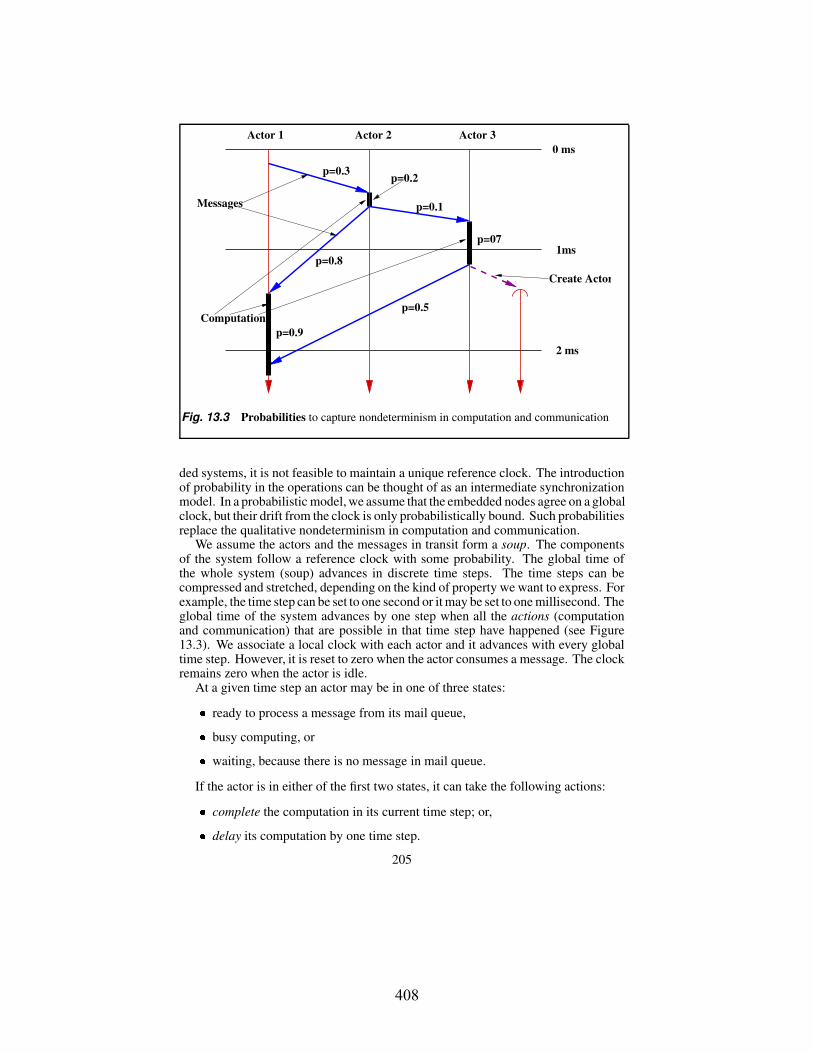
1ms

0 ms

2 ms

Actor 1 Actor 2 Actor 3

Computations

p=0.3

p=0.1

p=0.2

p=07

p=0.8

p=0.5

p=0.9

Create Actor

Messages

Fig. 13.3 Probabilities to capture nondeterminism in computation and communication

ded systems, it is not feasible to maintain a unique reference clock. The introductionof probability in the operations can be thought of as an intermediate synchronizationmodel. In a probabilistic model, we assume that the embedded nodes agree on a globalclock, but their drift from the clock is only probabilistically bound. Such probabilitiesreplace the qualitative nondeterminism in computation and communication.

We assume the actors and the messages in transit form a soup. The componentsof the system follow a reference clock with some probability. The global time ofthe whole system (soup) advances in discrete time steps. The time steps can becompressed and stretched, depending on the kind of property we want to express. Forexample, the time step can be set to one second or it may be set to one millisecond. Theglobal time of the system advances by one step when all the actions (computationand communication) that are possible in that time step have happened (see Figure13.3). We associate a local clock with each actor and it advances with every globaltime step. However, it is reset to zero when the actor consumes a message. The clockremains zero when the actor is idle.

At a given time step an actor may be in one of three states: ready to process a message from its mail queue, busy computing, or waiting, because there is no message in mail queue.

If the actor is in either of the first two states, it can take the following actions: complete the computation in its current time step; or, delay its computation by one time step.

205

408

In the first case, the local clock of the actor remains same and so it is open to otheractions in that time step. However, for the second action the local clock of the actoradvances by one time step and hence, all possible actions of that actor get disabled forthat time step. The two actions get enabled once the global time advances to the nexttime step. As a function of the state of the system, we associate different probabilitieswith each of the two actions.

Similarly, at a given time step a message can take three actions:

it can get enqueued at the target actor, it can get lost and thus removed from the soup, or it can get delayed, in transit, by one time step.

If a message is delayed in transit, the local time of the message advances by onetime step and so the message cannot take any more actions in that global time step.However, all the three actions will get enabled once the global time advances to thenext step. Probabilities are associated with each action. The probabilities depend onfactors such as the message density in the route taken by the message, the time forwhich it has been delayed (value of local clock of the message), and the number ofmessages sharing the same communication channel.

A computation path is defined as a sequence of states that the system has seen in thecourse of its computation. Note that the system retains the same computation pathsas it would have in a nondeterministic model of concurrency. The probability that aparticular finite sequence of states in a path will occur is obtained by multiplying theprobabilities of all the actions in that sequence of states. Some of these probabilitieswill grow sufficiently small that they will no longer be relevant to the proof of someproperties of our interest.

Using the above model, we can express properties of the form: “Within time,

the system will reach a state which satisfies a property with probability .” Forexample:

the alarm clock will ring at 7:00 a.m. with probability 0.99. the microwave will complete popping 95% of the popcorn by 10 a.m. with

probability 0.98.

In implementing probabilistic timing specifications, one constrains the system levelbehavior which involves networks of heterogeneous nodes. A middleware providesa uniform interface to access such nodes. We represent the middleware itself as acollection of actors. The model we describe enables dynamic customizability of theexecution environment of an actor in order to satisfy properties such as timing andsecurity.

13.3 REFLECTIVE MIDDLEWARE

A key requirement for middleware is that it must enable dynamic customization – sothat services can be pushed in and pulled out at runtime. This scheme of pushing-in and pulling-out of services allows the middleware to keep on a node only thoseservices that are required by an application. The result is a light weight middleware.

206

409

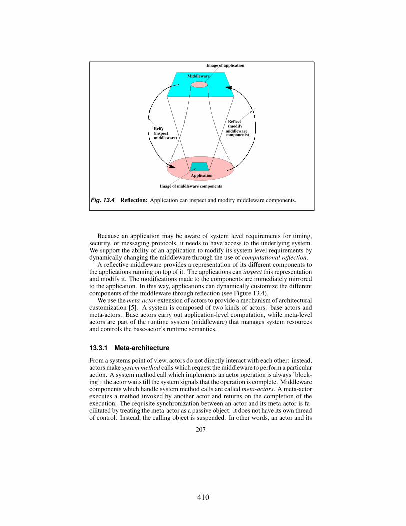
Application

Image of application

Middleware

Image of middleware components

Reify(inspect middleware)

(modifyReflect

components)middleware

Fig. 13.4 Reflection: Application can inspect and modify middleware components.

Because an application may be aware of system level requirements for timing,security, or messaging protocols, it needs to have access to the underlying system.We support the ability of an application to modify its system level requirements bydynamically changing the middleware through the use of computational reflection.

A reflective middleware provides a representation of its different components tothe applications running on top of it. The applications can inspect this representationand modify it. The modifications made to the components are immediately mirroredto the application. In this way, applications can dynamically customize the differentcomponents of the middleware through reflection (see Figure 13.4).

We use the meta-actor extension of actors to provide a mechanism of architecturalcustomization [5]. A system is composed of two kinds of actors: base actors andmeta-actors. Base actors carry out application-level computation, while meta-levelactors are part of the runtime system (middleware) that manages system resourcesand controls the base-actor’s runtime semantics.

13.3.1 Meta-architecture

From a systems point of view, actors do not directly interact with each other: instead,actors make system method calls which request the middleware to perform a particularaction. A system method call which implements an actor operation is always ’block-ing’: the actor waits till the system signals that the operation is complete. Middlewarecomponents which handle system method calls are called meta-actors. A meta-actorexecutes a method invoked by another actor and returns on the completion of theexecution. The requisite synchronization between an actor and its meta-actor is fa-cilitated by treating the meta-actor as a passive object: it does not have its own threadof control. Instead, the calling object is suspended. In other words, an actor and its

207

410

Actor

MetaActor

MetaActor

System MethodInvocation Path

Single Thread

Actor

MetaActor

MetaActor

System MethodInvocation Path

Single Thread

System

Node

Meta−level stacks

Message queueMessage queue

Fig. 13.5 Stacks of meta-level actors in an embedded node.

meta-actor are not concurrent – the latter represents the system level interpretation ofthe behavior of the former.

A meta-actor is capable of customizing the behavior of another actor by executingthe method invoked by it. An actor customized in this fashion is referred to as the baseactor relative to its meta-actor. To provide the most primitive model of customizationa meta-actor can customize a single base-actor. However, multiple customizationsmay be applied to a single actor by building a meta-level stack, where a meta-levelstack consists of a single actor and a stack of meta-actors (see Figure 13.5). Eachmeta-actor customizes the actor which is just below it in the stack. Messages receivedby an actor in a meta-level stack are always delegated to the top of the stack so thatthe meta-actor always controls the delivery of messages to its base-actor. Similarlymessages sent by an actor pass through all the meta-actors in the stack.

We identify each operation of a base-actor as a system method call as follows.

send(msg): This operation invokes the system method transmit with msg(msg is the message sent by the actor) as argument. If the actor has a meta-actor on its top it calls the transmit method of the meta-actor and wait for its

208

411

transmit(msg) create(beh) ready()

Meta−actor

ready()create(beh)send(msg)

msgbeh

()

Base Actor

() a

msg

Fig. 13.6 Interaction between meta-actor and base actor

return. The method returns without any value. Otherwise, if the actor is notcustomized by a meta-actor, it passes the message to the system for sending.

create(beh): This operation invokes the system method create with thegiven beh (beh is the behavior with which the newly created actor will beinstantiated) as argument. If there is a meta-actor on top of the actor, it calls thecreate method of the meta-actor and waits for its return. The method returnsthe address a of the new actor. Otherwise, the actor passes the create requestto the system.

ready(): The system method ready is invoked when an actor has completedprocessing the current message and is waiting for another message. If the actorhas a meta-actor on top it calls the ready method of the meta-actor and waitsfor its return. The method returns a message to the base-actor. Otherwise, theactor picks up a message from its mail queue and processes it. Notice, there isa single mail-queue for a given meta-level stack.

The method call-return mechanism for different actor operations and the availabil-ity of a single queue for a meta-level stack makes the execution of a meta-level stacksingle threaded. So explicit scheduling of each actor in the stack is not required. Themeta-actors behave as reactive passive objects which respond only when a systemmethod is invoked by its base actor. The single thread implementation of a meta-levelstack is important, as most of the embedded devices can have a single thread only.An example of such a embedded OS is TinyOS which runs on motes.

Every meta-actor has a default implementation of the three system methods. Theseimplementations may be described as follows:

209

412

transmit(msg): If there is a meta-actor on its top, it calls transmit(msg)method of that meta-actor and waits for it to return. Otherwise, it asks thesystem to send the message to the target and returns.

create(beh): If the actor has a meta-actor at its top, it calls create(beh)method of that meta-actor and waits for the actor to return with an actor address.Otherwise, the actor passes the create request to the system and waits till it getsan actor address from the system. After receiving new actor address, the actorreturns it to the base actor.

ready(): If there is a meta-actor on top of it, it calls ready() method ofthat meta-actor and waits for it to return a message. Otherwise, the actor, bydefinition located at the top of the meta-level stack, dequeues a message fromthe mail queue. After getting the message, the actor returns the message to thebase actor.

actor Encrypt(actor receiver)

// Encrypt outgoing// messages if they// are targeted to// the receivermethod transmit(Msg msg)

actor target = msg.dest;if (target == receiver)

target encrypt(msg);else

target msg;return;

actor Decrypt()

// Decrypt incoming messages// targeted for// base actor (if necessary)method ready()

Msg msg = ready();if (encrypted(msg))

return(decrypt(msg));else

return(msg);

Fig. 13.7 Meta-Level Implementation of Encryption: The Encrypt meta-actor inter-cepts transmit signals and encrypts outgoing messages. The Decrypt policy actor inter-cepts messages targeted for the receiver (via the rcv method) and, if necessary, decrypts anincoming message before delivering it.

As an example of how we may customize actors under this model, consider theencryption of messages between a pair of actors. Figure 13.7 gives pseudo-code fora pair of meta-actors which may be installed at each endpoint. The Encrypt meta-actor implements the transmit method which is called by the base-actor whilesending a message. Within transmit, a message is encrypted before it is sent toits target. The Decrypt meta-actor implements the ready method which is calledwhen the base actor is ready to process a message. Method ready decrypts themessage before returning the message to the base-actor.

The abstraction of the middleware in terms of meta-actors gives the power ofdynamic customization. Meta-actors can be installed or pulled out dynamically. Thispushing in and pulling out of meta-actors by the application itself makes it capable ofcustomizing the middleware. It also makes it possible to have only those middlewarecomponents which are required by services of the current application – facilitatingour goal of thin middleware.

210

413

Encrypt1MetaActor

Encrypt1MetaActor

Encrypt1Pulling out Pushing in

Encrypt2

BeforeAfter

Encrypt2MetaActor

Encrypt2MetaActor

Actor Actor

SystemSystem

Fig. 13.8 Dynamic Customization: Pulling out and pushing in a new meta-actor for theimplementation of encryption algorithm

13.4 DISCUSSION

We have described some preliminary work on a model of reflective middleware. Webelieve that further development of thin middleware will be central to the futureintegration of computing and the physical world [4]. However, many importantproblems have to be addressed before such an integration can be realized. We describetwo areas to illustrate the problems. These areas relate, respectively, to the model andimplementation of middleware.

A formal model of the interaction of the properties of actors and meta-actorshas been developed in terms of a two-level semantics [15]. This model needs tobe extended to its probabilistic real-time counterpart. For example, methods forcomposition of transition probabilities for actors and their meta-actors have not beendeveloped.

More research is required in the implementation of thin middleware. Currentimplementation of reflective actor middleware has been based on high-level languages– which necessarily assume a large infrastructure. An alternate implementation wouldbe in terms of a very efficient and small virtual machine which allows enforcement oftiming properties. Related problems are incrementally compiling high-level code tosuch a virtual machine and supporting the mobility of actors executing on the virtualmachine.

In our view, the solution to these and related problems define an ambitious researchagenda for the coming decade.

211

414

13.5 ACKNOWLEDGMENTS

The research described here has been supported in part by the Defense AdvancedResearch Projects Agency (Contract numbers: F30602-00-2-0586 and F33615-01-C-1907). We would like to thank Nadeem Jamali and Nirman Kumar for reviewingprevious versions of this paper and giving feedback.

REFERENCES

1. G. Agha. Actors: A Model of Concurrent Computation. MIT Press, 1986.

2. G. Agha. Modeling Concurrent Systems: Actors, Nets, and the Problem ofAbstraction and Composition. In 17th International Conference on Applicationand Theory of Petri Nets, Osaka, Japan, June 1996.

3. G. Agha, I. A. Mason., S. F. Smith, and C. L. Talcott. A foundation for actorcomputation. Journal of Functional Programming, 7:1–72, 1997.

4. Gul A. Agha. Adaptive middleware. Communications of the ACM, 45(6):30–32,June 2002.

5. M. Astley and G. Agha. Customization and composition of distributed objects:Middleware abstractions for policy management. In Proceedings of the SixthInternational Symposium of Foundations of Software Engineering, pages 1–9,1998.

6. S. B. Fuller, E. J. Wilhelm, and J. M. Jacobson. Ink-jet printed nanoparticlemicroelectromechanical systems. Journal of Microelectromechanical Systems,11(1):54–60, 2002. http://www.media.mit.edu/molecular/projects.html.

7. AIM. Inc. http://www.aimglobal.org/technologies/rfid/.

8. J. M. Kahn, R. H. Katz, and K. S. J. Pister. Mobile Networking for Smart Dust.In ACM/IEEE Intl. Conf. on Mobile Computing and Networking (MobiCom 99),Seattle, WA, August 1999. http://robotics.eecs.berkeley.edu/ pister/SmartDust/.

9. MIT Media Lab. http://lcs.www.media.mit.edu/projects/wearables/.

10. B. Nielsen and G. Agha. Semantics for an Actor-Based Real-Time Language.In 4th International Workshop on Parallel and Distributed Real-Time Systems(WPDRTS). Submitted. Naval Surface Warfare Center Dahlgren Division/IEEE,April 1995. In conjunction with 10th IEEE Int. Parallel Processing Symposium(IPPS), Honolulu, Hawaii, USA.

11. B. Nielsen and G. Agha. Towards reusable real-time objects. Annals of SoftwareEngineering: Special Volume on Real-Time Software Engineering, 7:257–282,1999.

12. D. Norman. The Invisible Computer. The MIT Press, Cambridge, MA, USA,1998.

212

415

13. S. Ren. An Actor-Based Framework for Real-Time Coordination. PhD thesis,Department Computer Science. University of Illinois at Urbana-Champaign,1997. PhD. Thesis.

14. S. Ren, G. Agha, and M. Saito. A modular approach for programming distributedreal-time systems. Journal of Parallel and Distributed Computing, 36(1):4–12,1996. Also published in School on Embedded Systems, European EducationalForum 1996, pp 52–72.

15. Nalini Venkatasubramanian and Carolyn L. Talcott. Reasoning about meta levelactivities in open distributed systems. In Symposium on Principles of DistributedComputing, pages 144–152, 1995.

Author(s) affiliation: Koushik Sen, and Gul Agha

Department of Computer ScienceUniversity of Illinois at Urbana-ChampaignEmail: [ksen,agha]@uiuc.edu

213

416