A parallel multigrid method for large A parallel multigrid method for large scale illscale ill--posed inverse problemsposed inverse problems

Volkan Akcelik, Stanford Linear Accelerator CenterVolkan Akcelik, Stanford Linear Accelerator CenterGeorge Biros, University of PennsylvaniaGeorge Biros, University of PennsylvaniaAndrei Dragenescu, Sandia National LabsAndrei Dragenescu, Sandia National LabsPearl Pearl FlathFlath, University of Texas, University of TexasOmar Ghattas, University of TexasOmar Ghattas, University of TexasJudy Hill, Sandia National LabsJudy Hill, Sandia National LabsBart van Bloemen Waanders, Sandia National LabsBart van Bloemen Waanders, Sandia National LabsKaren Karen WillcoxWillcox, MIT, MIT

Model problem: inversion for initial Model problem: inversion for initial condition of contaminant transportcondition of contaminant transport

transport equation

data misfit at sensors regularizationState and control

Typical scenario:

• Greater Los Angeles Basin• Airflow from mesoscopicweather model (e.g. MM5)• Sensor readings of contaminant concentration• Invert for “initial condition”• Repeat on moving window

Challenge:• rapid turnaround• high resolution models• real-time data• ! fast scalable inverse algorithms

Inversion-based reconstruction of initial condition

“Real” initial condition

Comparison over time of transport of actual Comparison over time of transport of actual plume with inversionplume with inversion--based predictionbased prediction

Inversion using 120 min time window; prediction for subsequent 1Inversion using 120 min time window; prediction for subsequent 150 min50 min

Back to inverse formulationBack to inverse formulation

Optimality conditions:Optimality conditions:

Block elimination

Solve for u in terms of u0

Solve for u0

Solve for p in terms of u

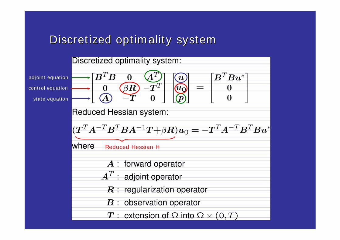
Discretized optimality systemDiscretized optimality system

state equationstate equation

adjoint equationadjoint equation

control equationcontrol equation

Reduced Hessian H

How to solve reduced Hessian system?How to solve reduced Hessian system?

•• Reduced Hessian is nonReduced Hessian is non--local operatorlocal operator•• For largest example, For largest example, H H is 135 million x 135 million dense is 135 million x 135 million dense

matrix; would require 10matrix; would require 1023 23 bytes memory, 400 yrs bytes memory, 400 yrs computing time (on PSC computing time (on PSC AlphaClusterAlphaCluster) to form) to form

•• Instead solve system by conjugate gradients; form matrixInstead solve system by conjugate gradients; form matrix--vector products on the flyvector products on the fly

•• Each Each matvecmatvec amounts to one forward + one adjoint solveamounts to one forward + one adjoint solve•• Parallelizes as well as the forward solverParallelizes as well as the forward solver•• But essential that convergence is rapid But essential that convergence is rapid –– is this guaranteed? is this guaranteed?

CG for forward (differential) operatorCG for forward (differential) operator

Spectrum of discrete Spectrum of discrete laplacianlaplacian

Eigenvector forEigenvector forsmall eigenvaluesmall eigenvalue

Eigenvectors for Eigenvectors for large eigenvaluelarge eigenvalue

CG for inverse (CG for inverse (FredholmFredholm integralintegral--like) operatorlike) operator

Spectrum of discrete reduced HessianSpectrum of discrete reduced Hessian

Eigenvector forEigenvector forsmall eigenvaluesmall eigenvalue

Eigenvector forEigenvector forintermediate eigenvalueintermediate eigenvalue

Eigenvector forEigenvector forlarge eigenvaluelarge eigenvalue

Discretization/solver detailsDiscretization/solver details

•• Velocity field computed by laminar Velocity field computed by laminar NavierNavier--Stokes codeStokes code•• MatrixMatrix--free conjugate gradient solution of reduced free conjugate gradient solution of reduced

Hessian system (each Hessian system (each matvecmatvec requires forward/adjoint requires forward/adjoint transport solution)transport solution)

•• Forward/adjoint transport equation discretized by Forward/adjoint transport equation discretized by SUPG/P1 FE in space, CrankSUPG/P1 FE in space, Crank--Nicolson in timeNicolson in time

•• Additive SchwarzAdditive Schwarz--preconditioned GMRES linear solver at preconditioned GMRES linear solver at each transport time stepeach transport time step

•• Adjoints needed only at initial time in inversion Adjoints needed only at initial time in inversion equation; states needed only at sensor locations to equation; states needed only at sensor locations to compute adjoints (i.e. no need for compute adjoints (i.e. no need for checkpointingcheckpointing))

•• PETSc library (Argonne) parallel implementation for PETSc library (Argonne) parallel implementation for forward preconditioners, linear solvers, parallel data forward preconditioners, linear solvers, parallel data structuresstructures

LA Basin example detailsLA Basin example details

•• Surface elevations obtained from USGS GTOPO30 digital Surface elevations obtained from USGS GTOPO30 digital elevation model at 1 km resolution elevation model at 1 km resolution

•• LA Basin region domain covers 360 km x 120 km x 5 km at LA Basin region domain covers 360 km x 120 km x 5 km at (horizontal) 1 km grid size (max elevation = 3.5 km)(horizontal) 1 km grid size (max elevation = 3.5 km)

•• TopographyTopography--conforming logicallyconforming logically--rectangular splitrectangular split--hexhex--based linear tetrahedral mesh based linear tetrahedral mesh oo 361361××121121××21 = 917,301 grid points21 = 917,301 grid pointsoo ≈≈ 74M total space74M total space--time variablestime variables

•• GaussianGaussian--shaped plume:shaped plume:oo uu00 = 20exp(= 20exp(--0.04|x0.04|x--xxcc|)|)oo centered at centered at xxcc = (120,60,0) km= (120,60,0) km

•• Inflow:Inflow:oo vvmaxmax(z/(5.0(z/(5.0--zzsurfacesurface))))0.10.1

oo vvmaxmax = 30 km/hr = 30 km/hr

•• Sensor readings every 3 minutes for 120 minute simulationSensor readings every 3 minutes for 120 minute simulation•• Run on 64 processors of Run on 64 processors of AlphaClusterAlphaCluster at PSCat PSC

Numerical studies of inversion sensitivity Numerical studies of inversion sensitivity Baseline case: Baseline case: kk = 0.05, = 0.05, ββ=0.01, =0.01, ηη = 0%, sensor = 11= 0%, sensor = 1133

1.1. Density of sensor array Density of sensor array oo 6 6 ×× 6 6 ×× 6, 11 6, 11 ×× 11 11 ×× 11, 21 11, 21 ×× 21 21 ×× 2121

2.2. Regularization parameterRegularization parameteroo ββ = 1, 0.1, 0.01, 0.001= 1, 0.1, 0.01, 0.001

3.3. PecletPeclet numbernumberoo kk = 0.05, 0.1, 0.2, 0.4= 0.05, 0.1, 0.2, 0.4oo i.e. i.e. PePe = 10, 5, 2.5, 1.25= 10, 5, 2.5, 1.25

4.4. Noise level of observationsNoise level of observationsoo ηη = 0%, 5%, 10%= 0%, 5%, 10%

1. Sensitivity to sensor array density1. Sensitivity to sensor array density

1. Sensitivity of initial condition inversion 1. Sensitivity of initial condition inversion to sensor array densityto sensor array density

2. Sensitivity to regularization parameter 2. Sensitivity to regularization parameter ββ

2. Sensitivity of initial condition inversion 2. Sensitivity of initial condition inversion to regularization parameter to regularization parameter ββ

3. Sensitivity to diffusivity 3. Sensitivity to diffusivity kk

3. Sensitivity of initial condition inversion 3. Sensitivity of initial condition inversion to diffusivity to diffusivity kk (i.e. ~1/Peclet number) (i.e. ~1/Peclet number)

4. Sensitivity to noise level 4. Sensitivity to noise level ηη

4. Sensitivity of initial condition inversion 4. Sensitivity of initial condition inversion to noise level to noise level ηη

Multigrid Multigrid preconditionerpreconditioner for reduced Hessian for reduced Hessian

•• UnpreconditionedUnpreconditioned (or (or (ββ RR)--11 preconditioned) CG is preconditioned) CG is optimal for reduced Hessian optimal for reduced Hessian –– number of iterations is number of iterations is mesh independentmesh independent

•• However, mesh independence is not good enough However, mesh independence is not good enough ––need to reduce constant! need to reduce constant!

•• Problem: need effective Problem: need effective preconditionerpreconditioner that does not that does not require H to be explicitly formedrequire H to be explicitly formed

•• Standard multigrid smoothers Standard multigrid smoothers not appropriatenot appropriate•• Appeal to multigrid ideas for regularized compact Appeal to multigrid ideas for regularized compact

operators (integral equations of the second kind)operators (integral equations of the second kind)oo W. W. HackbushHackbush, 1985, 1985oo J.T. King, 1992J.T. King, 1992oo M. M. HankeHanke and C. Vogel, 1999and C. Vogel, 1999oo B. B. KaltenbacherKaltenbacher, , ……, 2003, 2003oo A. A. DraganescuDraganescu, 2004, 2004

Multigrid Multigrid preconditionerpreconditioner

Multigrid Multigrid preconditionerpreconditioner, implementation, implementation

Parallel multigrid performance and Parallel multigrid performance and scalability on PSC EV68 scalability on PSC EV68 AlphaClusterAlphaCluster

Fixed size scalabilityFixed size scalability:: 257 x 257 x 257 x 257 space257 x 257 x 257 x 257 space--time time grid; 17 million inversion parameters, 8.7 billion total spacegrid; 17 million inversion parameters, 8.7 billion total space--time unknowns; 3time unknowns; 3--level level preconditionerpreconditioner; parallelism in space ; parallelism in space but not timebut not time

IsogranularIsogranular scalabilityscalability: fixed spatial problem size per processor : fixed spatial problem size per processor as # of processors increases (largest problem has 135 million as # of processors increases (largest problem has 135 million inversion parameters, ~140 billion total spaceinversion parameters, ~140 billion total space--time unknowns) time unknowns) (95% parallel efficiency on 128 (95% parallel efficiency on 128 PEsPEs; 86% on 1024 ; 86% on 1024 PEsPEs))

Uncertainty quantification = Uncertainty quantification = input uncertainty estimation + propagationinput uncertainty estimation + propagation

•• Two steps:Two steps:1.1. Estimate uncertainty in inputs from measurements of the Estimate uncertainty in inputs from measurements of the

observables (statistical inverse problem)observables (statistical inverse problem)2.2. Propagate input uncertainties through the simulation to Propagate input uncertainties through the simulation to

predict uncertainties in output quantities of interest predict uncertainties in output quantities of interest •• Application to transport of airborne contaminants: Application to transport of airborne contaminants:

1.1. Inverse problem:Inverse problem:oo Governing equation is a scalar convectionGoverning equation is a scalar convection--diffusion diffusion

equationequationoo Uncertain field is the initial condition Uncertain field is the initial condition oo Observables are contaminant concentrations at a sparse Observables are contaminant concentrations at a sparse

set of sensorsset of sensorsoo Inverse problem is to determine mean and (Inverse problem is to determine mean and (co)varianceco)variance

of initial condition field given contaminant observations of initial condition field given contaminant observations at sensorsat sensors

2.2. Uncertainty propagation:Uncertainty propagation:oo Input uncertainty in initial condition obtained from Input uncertainty in initial condition obtained from

inverse probleminverse problemoo Output quantity of interest is evolution (mean, variance) Output quantity of interest is evolution (mean, variance)

of contaminant concentration over timeof contaminant concentration over time

Estimation of uncertainty in initial Estimation of uncertainty in initial condition from inverse solutioncondition from inverse solution

•• MCMC Bayesian estimation framework is prohibitive for MCMC Bayesian estimation framework is prohibitive for such problems (millions of parameters)such problems (millions of parameters)

•• Assuming Gaussian statistics (for uncertainty in Assuming Gaussian statistics (for uncertainty in measurements, model errors, and initial conditions) and measurements, model errors, and initial conditions) and for linear inverse problems, covariance of initial for linear inverse problems, covariance of initial conditions given by inverse of Hessian matrixconditions given by inverse of Hessian matrix

•• Hessian is impossible to form (e.g. 400 yrs of Hessian is impossible to form (e.g. 400 yrs of computing time), let alone invertcomputing time), let alone invert

•• Create low rank approximation of compact part of Create low rank approximation of compact part of HessianHessian

•• Use ShermanUse Sherman--MorrisonMorrison--Woodbury formula to invert Woodbury formula to invert Hessian approximation to give covariance of initial Hessian approximation to give covariance of initial conditioncondition

•• Cost is order of inverse problem solveCost is order of inverse problem solve

Compact structure of Hessian operatorCompact structure of Hessian operator

Spectrum of discrete reduced HessianSpectrum of discrete reduced Hessian

Eigenvector forEigenvector forsmall eigenvaluesmall eigenvalue

Eigenvector forEigenvector forintermediate eigenvalueintermediate eigenvalue

Eigenvector forEigenvector forlarge eigenvaluelarge eigenvalue

Influence of eigenvalue cutoff for lowInfluence of eigenvalue cutoff for low--rank approximation of Hessianrank approximation of Hessian

Cutoff= 0.1Cutoff= 0.1

# # eigseigs = 36= 36

Cutoff= 0.001Cutoff= 0.001

# # eigseigs = 210= 210

Cutoff= 0.01Cutoff= 0.01

# # eigseigs = 123= 123

Cutoff= 0.0001Cutoff= 0.0001

# # eigseigs = 264= 264

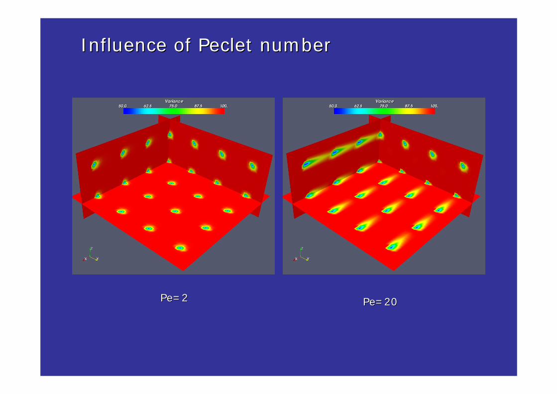
Influence of Influence of PecletPeclet numbernumber

PePe=2=2 PePe=20=20

Influence of number of sensorsInfluence of number of sensors

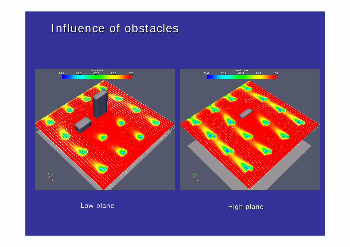
Influence of obstaclesInfluence of obstacles

Low planeLow plane High planeHigh plane

Forward propagation of contaminantForward propagation of contaminant

SummarySummary

•• Simplified model of atmospheric transportSimplified model of atmospheric transportoo Velocity field assumed known Velocity field assumed known oo No depositionNo depositionoo No chemical reactionsNo chemical reactions

•• Excellent overall (algorithmic + parallel) Excellent overall (algorithmic + parallel) isogranularisogranularscalability of parallel multigrid scalability of parallel multigrid preconditionerpreconditioner

•• ~135 million inversion parameter problem solved in ~135 million inversion parameter problem solved in <5h on 1024 Alpha processors <5h on 1024 Alpha processors

•• Low rank structure of Hessian can be exploited to Low rank structure of Hessian can be exploited to estimate covariance matrix of initial condition unknowns estimate covariance matrix of initial condition unknowns in cost proportional to solving inverse problemin cost proportional to solving inverse problem

•• Initial condition uncertainty can be propagated readily Initial condition uncertainty can be propagated readily with low rank with low rank

AcknowledgmentsAcknowledgments

•• TOPS Center: Terascale Optimal PDE SimulationsTOPS Center: Terascale Optimal PDE Simulations((www.topswww.tops--scidac.orgscidac.org))oo Supported under DOE SciDAC/ISIC programSupported under DOE SciDAC/ISIC programoo Collaboration with LLNL, ANL, LBNL + 8 universitiesCollaboration with LLNL, ANL, LBNL + 8 universities

•• Computer Science Research Institute, SandiaComputer Science Research Institute, Sandia

•• Caliente Project: Dynamic Inversion and ControlCaliente Project: Dynamic Inversion and Control((www.cs.cmu.edu/~calientewww.cs.cmu.edu/~caliente) ) oo NSF/ITR ACINSF/ITR ACI--01216670121667oo Other collaborators: L. Biegler (CMU), D. Keyes (ODU), Other collaborators: L. Biegler (CMU), D. Keyes (ODU),

M.HeinkenschlossM.Heinkenschloss (Rice), R. Bartlett (Sandia), D. Young (Boeing), F. (Rice), R. Bartlett (Sandia), D. Young (Boeing), F. FendellFendell (TRW), A. (TRW), A. WaechterWaechter (IBM)(IBM)

•• Quake ProjectQuake Project (NSF/ITR EAR(NSF/ITR EAR--0326449)0326449)•• Cardiac Inversion ProjectCardiac Inversion Project (NSF/ITR CCF(NSF/ITR CCF--0427985)0427985)•• Special thanks to staff atSpecial thanks to staff at Pittsburgh Supercomputing Pittsburgh Supercomputing

CenterCenter (NSF (NSF TeraGridTeraGrid award MCA01S002P)award MCA01S002P)•• Special thanks to Special thanks to PETSc groupPETSc group at Argonne (S. at Argonne (S. BalayBalay, K. , K.

BuschelmanBuschelman, W. , W. GroppGropp, D. , D. KaushikKaushik, M. , M. KnepleyKnepley, L. , L. McInnesMcInnes, B. Smith, H. Zhang), B. Smith, H. Zhang)