Embed Size (px)
Citation preview
Project Number: CS-DCB-0901
A PARALLEL EMBEDDED NEURAL NETWORK FOR AN INTELLIGENT TURN-BASED GAME ENGINE
A Major Qualifying Project Report:
submitted to the Faculty
of the
WORCESTER POLYTECHNIC INSTITUTE
in partial fulfillment of the requirements for the
Degree of Bachelor of Science
by
__________________________________ ___________________________________
Stephen Mann Matthew Netsch ECE ECE/CS
Date: May 03, 2010
Approved:
______________________________________
Professor David C. Brown, CS Major Advisor
1. Neural Network 2. Embedded 3. Parallel
_______________________________________
Professor Stephen J. Bitar, ECE Major Advisor

Error! Reference source not found. 2
Abstract The purpose of this project was to design a parallel digital circuit that performs neural network (NN) calculations more efficiently than traditional software implementations, by taking advantage of the NN's inherent parallel structure. User interfaces for NN training and testing were developed. Tic-Tac-Toe position evaluation was used as a test domain. Testing showed that the parallel hardware NN decreased the number of required clock cycles by an order of magnitude.

Error! Reference source not found. 3
Contents Abstract ......................................................................................................................................................... 2
Contents ........................................................................................................................................................ 3
1 Introduction .......................................................................................................................................... 5
1.1 Problem Statement ....................................................................................................................... 5
1.2 Background ................................................................................................................................... 6
1.2.1 The Neural Network Model .................................................................................................. 6
1.2.2 Forward Propagation ............................................................................................................ 7
1.2.3 Negamax ............................................................................................................................. 10
1.2.4 Back-Propagation ................................................................................................................ 11
1.3 Requirements and Goals ............................................................................................................. 17
1.3.1 Parallel Neural Network Design .......................................................................................... 18
1.3.2 Software Evaluation Tool .................................................................................................... 18
1.3.3 Verify Parallel System Efficiency and Correctness .............................................................. 19
2 Design .................................................................................................................................................. 20
2.1 General System ........................................................................................................................... 20
2.1.1 TAC ...................................................................................................................................... 20
2.1.2 Software Driver ................................................................................................................... 21
2.1.3 Hardware Driver .................................................................................................................. 21
2.1.4 Hardware NN ...................................................................................................................... 22
2.2 Trainer, Analyzer, Controller ....................................................................................................... 22
2.2.1 Network Tab ........................................................................................................................ 24
2.2.2 Device Tab ........................................................................................................................... 27
2.2.3 Test Tab ............................................................................................................................... 28
2.2.4 Train Tab ............................................................................................................................. 31
2.2.5 Developing for TAC ............................................................................................................. 33
2.2.6 File Specifications ................................................................................................................ 40
2.3 Parallel Neural Network .............................................................................................................. 40
2.3.1 Parallel Structure Analysis................................................................................................... 40

Error! Reference source not found. 4
2.3.2 Efficiency ............................................................................................................................. 41
2.3.3 Neuron ................................................................................................................................ 42
2.4 Hardware and Software Driver ................................................................................................... 52
2.4.1 Software Driver ................................................................................................................... 53
2.4.2 Hardware Driver .................................................................................................................. 54
2.4.3 Message Types .................................................................................................................... 56
2.4.4 Connection Protocol ........................................................................................................... 61
2.4.5 Registers .............................................................................................................................. 62
2.4.6 Driver Tester Interface ........................................................................................................ 64
3 Analysis ............................................................................................................................................... 69
3.1 Hardware Neural Network .......................................................................................................... 69
3.1.1 Neuron State ....................................................................................................................... 69
3.1.2 Switch .................................................................................................................................. 70
3.1.3 Multiplier ............................................................................................................................. 71
3.1.4 Accumulator ........................................................................................................................ 72
3.1.5 Sigmoid ................................................................................................................................ 73
4 Conclusion ........................................................................................................................................... 82
5 References .......................................................................................................................................... 85
6 Appendix A- Distribution of work ....................................................................................................... 86
6.1 Stephen Mann ............................................................................................................................. 86
6.1.1 Deliverables ......................................................................................................................... 86
6.1.2 Paper ................................................................................................................................... 86
6.2 Matthew Netsch ......................................................................................................................... 86
6.2.1 Deliverables ......................................................................................................................... 86
6.2.2 Paper ................................................................................................................................... 86
7 Appendix B - Lessons Learned............................................................................................................. 87
7.1 Steve ............................................................................................................................................ 87
7.2 Matt ............................................................................................................................................ 87

1 Introduction The purpose of this project is to design an efficient hardware neural network (NN) and to apply this NN to solving a real world problem: playing Tic-Tac-Toe. Common computer implementations of artificial NN’s are inefficient due to the sequential nature of their processors, which can only execute one calculation at a time; artificial NN’s contain, due to their parallel nature, many independent calculations which can be executed simultaneously on custom hardware to greatly improve the efficiency.
This project will be designed to run on a Field Programmable Gate Array (FPGA). FPGA’s are hardware devices that can be programmed to implement custom digital designs by physically mapping paths between the logic gates on each device. Using an FPGA allows the structure of the NN to be reprogrammed without any monetary cost.
The FPGA containing the NN design will be able to receive inputs and to send output results to a common computer through a Universal Serial Bus (USB) interface. This connection allows software to communicate with the FPGA NN, enabling the software to perform NN calculations using the connected device.
All of these components will be combined and used to play Tic-Tac-Toe, a turn based board game. Evaluating Tic-Tac-Toe positions using the FPGA will verify that the hardware design correctly implements the artificial NN algorithm and that the accuracy of the hardware implementation of the artificial NN is satisfactory.
Once all of these parts are designed and integrated, the performance of both the hardware NN and a software NN will be compared to determine the efficiency improvement of the hardware implementation over the software implementation.
1.1 Problem Statement Artificial NN’s are models used to simulate the human brain (Orr 1999). These simulations, while far from accurately modeling a biological brain, have been proven to be effective at pattern classification and are commonly used for image processing and speech recognition (Li 1990). However, the complexity of NN’s makes them inefficient to compute using modern processors.
Computers are useful tools for solving problems written in a sequential algorithmic form. However, NN models cannot be efficiently written in such a way. The problem lies in the massively parallel structure of the NN, as each of its parallel connections must be computed in sequence in order to produce its output.
There are ways to distribute work with computers and simulate parallelism. However, for the size of a NN model for a small application such as Tic-Tac-Toe, this would require many physical processor cores. A common application such as image processing would require on the order of thousands of cores. Further, to make matters worse, many NN applications would be useful in mobile devices where

Introduction 6
processing resources are limited. Solutions neglecting the benefit of true parallelism are therefore currently infeasible without substantial computing power.
Part of the problem is that computer processors are designed to be generic problem solvers. This makes them inefficient and expensive for this specific parallel application. A processor especially designed to carry out NN operations would make this more efficient. This technique of distributing specialized computation is commonly used in devices such as video cards for rendering graphics and sound cards for processing sound. Our work involves designing a custom processor for providing the parallel computations of a NN model.
1.2 Background An artificial NN is modeled after the human brain (Orr 1999). Artificial neural networks are computational models which can be trained to recognize patterns, known as a pattern classifier. What makes this particular pattern classifier useful is that, if trained correctly, it can apply previous knowledge to unencountered situations and produce a satisfactory result. For example, in the application of image processing, a NN can be trained to recognize tanks looking at images from an unmanned air vehicle (UAV) (Bianchini, et al. 2004). However, most classifier algorithms over-fit what they were trained to recognize. In other words, they can classify objects they have seen before very well, but not if the object is in a slightly different situation. In the UAV application, if the NN was trained with images of tanks from a military base, but the UAV is operating in the desert, the lighting will be different enough to make other classifiers not work effectively.
1.2.1 The Neural Network Model Many neurons are arranged together in the brain in a complex network. A single neuron acts as a valve to change the flow of information propagating through the NN. Neurons will strengthen some signals and limit others in order to produce the final resulting output. In a brain, neurons collect inputs like water flowing into a dam. When the water attains a certain predefined level, it empties everything into its outputs and starts over again.
Figure 1 – A biological neural network (left); a simulated computer model (right)

Introduction 7
The model shown in Figure 1 is called a multi-layered perceptron. This special type of NN is feed-forward, meaning that there are no loops in the directed graph. This also means that the neurons are grouped into layers and that every neuron in a layer is connected to every neuron in the layer after it. This simple model consists of three layers; an input layer, a hidden layer, and finally an output layer. In order to simulate the limiting of the signal that the biological model has, connections are assigned coefficients, called weights, each of which multiplies any signal passing through it. Once all of the signals from input connections to a neuron are obtained, the resulting value is summed. The neuron takes this
sum and applies a sigmoid activation function to it, commonly a hyperbolic tangent or , where ‘x’ is
the sum of the inputs to the neuron. This function limits the output of the neuron, and its result is then applied to each output connection. Each output connection then scales the value applied to it, leading into its output neuron as an input.
Figure 2 – The Neuron Model
1.2.2 Forward Propagation The application that we use our NN for is a common technique called curve fitting. Curve fitting is the process of determining a function that closely matches a given set of input, output pairs. Neural networks are good at doing this because they are able to recognize patterns in the data set and fill in the missing information between each data point. Figure 3 shows a simple neural network to use as an example. This NN will be used to fit a third order polynomial.

Introduction 8
Figure 3 – The simple neural network (left); Target function to fit (right)
When adjusted, the connection weights in the NN cause its output to change shape. That is, the weights along the NN’s connections can be chosen in such a way that the output of the neural network resembles a specific cubic function when its input varies. The goal of training a network is to adjust its weights in such a way that the output function closely matches the training data. The process of how a neural network produces its output from its given inputs is called forward propagation.
As shown before, each simulated neuron has the output function:
Eq 1.1
Eq 1.2
Therefore, after some algebra, the equation of the final output of the example neural network in Figure 3 is:
Eq 1.3
The weights act as the neural network’s memory and will cause the neural network to produce the target cubic function when chosen correctly. Techniques for determining weights that allow the neural

Introduction 9
network to approximate functions will be discussed in section 1.2.4. The target function we are trying to approximate for this example is:
Eq 1.4
Though it is beyond the scope of this section, we decided to use the sigmoid of f(x) as the target function. This choice had to do with problems obtaining negative output values when determining weights. Therefore, after training the NN to approximate the sigmoid of f(x), we applied the inverse of the sigmoid on the output of the neural network to obtain the original f(x). The weights that allow this neural network to produce a good approximate of f(x) over the arbitrarily chosen bounds of -0.9 to 0.5 are:
The simplified output equation of the neural network becomes:
where
out(x) above is about equivalent to f(x) over the range -0.9 to 0.5. Note that the input vector, ‘i,’ contains a second term that is always one. This input value is constant, and is passed through to the next layer because no sigmoid function is applied to the input neuron. The output of this neuron shifts the output of the entire network by a nearly constant value, helping to offset the output function in a way that might be difficult for the varying input terms. Figure 4 demonstrates how the neural network produces out(x).
Figure 4-Forward Propagation

Introduction 10
For the weights chosen, the output produced by the neural network when given x = -0.2 is 0.50128. Remember, as stated previously, that the out(x) function must have the inverse sigmoid applied to it. The actual result is therefore 0.0051, and when compared to the expected value of 0 it has a root mean squared (RMS) error of only 1.64E-6. This value is calculated by taking the square root of the sum of all squared output errors, where the errors are calculated by subtracting the actual output from the expected output. Given a set of input, output pairs, the neural network performs well, producing outputs with an RMS error of only 1.34746E-5. Determining the weights that will produce the expected output is a topic for later.
1.2.3 Negamax Our work uses a neural network to perform a function approximation of a function called Negamax. Negamax is a recursive function that evaluates a game position and returns a value representing the favorability of the position with respect to the current player. Using Negamax even for simple games such as Tic-Tac-Toe requires a lot of recursion and on a modern computer can take up to a couple seconds to produce a result.
The underlying data structure of the Negamax algorithm is a game tree. At the root of a game tree is the first position in the game to be analyzed. Each branch of the root node represents a position possible to reach by making a single move in the root position. The same properties are true for each node in the game tree—the child positions represent possible positions resulting from their parent positions. All leaf nodes in a game tree represent positions in which the game has ended.
Figure 5 – Section of the Tic Tac Toe game tree (left); Negamax output as a function (right)
Although Tic-Tac-Toe has a game tree with hundreds of thousands of different positions, there are only 4804 unique board positions. The graph in Figure 5 only shows these unique board positions on the x axis (indexed). The expected output for the Tic-Tac-Toe function is shown on the y axis for the given

Introduction 11
board position. This is the function our neural network should approximate. The diagram in the Figure 5 on the left shows how Negamax evaluates up the game tree from the leaf nodes.
Negamax produces its result by traversing through the entire game tree. When the algorithm hits a leaf node it assigns it a 1 for the current player winning, a 0 for draw, and a -1 for the current player losing. Whether or not the position is win or a loss is decided from the context of the next player to move. For example, if X was the last player to place and resulted in a win then the result would be -1 as it is a loss for the next player to place an O. The node directly above the leaf node will take the inverse of the scores all of its children and assign itself the greatest of these values. This occurs until the root node is reached.
Our algorithm takes the score of the root node and assigns a 0.8333 if -1 is returned, 0.5 if 0 is returned, and 0.1667 if 1 is returned. These values are chosen to help with the training and will be explained later.
Figure 6 - Tic-Tac-Toe Game Tree Growth
The number of recursive Negamax function calls is on the order of hundreds of thousands seen in Figure 6, even for a small game tree generated from Tic-Tac-Toe. However, a NN would only require a fixed number of multiplications and a handful of sigmoid calculations to get close to the same result. The Negamax algorithm grows exponentially with the depth of the tree it searches. Therefore, the neural network is a more efficient way of producing this result, since it always takes the same amount of time to execute. This assumes we have the correct weights to produce the Negamax function, which are obtained through using the back-propagation algorithm.
1.2.4 Back-Propagation A neural network must be trained before it produces meaningful results. Most problems require neural networks with different structures, which require that there be some way to generate a network structure relevant to a problem. The size of a network—the number of neurons and the number of
1
10
100
1000
10000
100000
1000000
0 2 4 6 8 10
Size
of G
ame
Tree
Number of Moves Left to Make
Tic-Tac-Toe Game Tree Growth

Introduction 12
interconnected neurons—must be chosen specifically for a problem. Once this structure is determined, the weights of the connections between neurons must then be adjusted such that the output of the NN matches its expected output.
The goal of adjusting the weights in a NN is to reduce the NN’s output error. Given a set of correct inputs and outputs, the network produces a corresponding set of outputs. The difference between the given outputs and the NN’s outputs is the error, represented by:
Eq 1.5
If is adjusted such that , then the network will have a perfect fit to the set of expected outputs. In most cases, this is computationally infeasible to calculate due to the large number of neurons and weights resulting in the need to solve a set of large multivariable equations. So instead of finding the global minimum error, most training algorithms attempt to find a local minimum resulting in an error below a predetermined threshold.
Local minima and maxima of the error function are found at the points of a curve where the derivative is equal to zero. To find those points, the derivative of the error function must be determined.
A neural network trained to find the best-fit line for a given set of data is a simple example of this.
Eq 1.6
Since this network is designed to fit a line, an activation function of is used. This significantly simplifies the output of the NN by making it linear. For example, the output of a simple three neuron NN
with two output neurons, is represented by , where
and are the inputs to the network and is the output.Similarly, the general neuron output equation simplifies to:
Eq 1.7
The gradient of the error function with respect to its weights points in the direction of steepest error increase. The opposite vector gives the direction of steepest decrease. Interpolating weights along this vector results in a smaller error, giving new weights of:

Introduction 13
Eq 1.8
The error gradient derivation:
Eq 1.9
Now there is enough information to calculate the weight changes for the entire network. The final weight update is:
Eq 1.10
The network in Figure 7, a network specifically designed to model the equation , uses this weight update rule and a linear activation function to find the best fit line for a set of data points. The weights of the network are represented by “m” and “b,” and the inputs are the coefficients of these weights, “x” and “1,” respectively.

Introduction 14
Figure 7 -Best fit line neural network
In order to test the effectiveness of the linear weight update rule, a set of data points following the line
is used as training data. A plot of the network output after each pass over the data set is shown
in Figure 8.
Figure 8 - Linear fit neural network output over time
Each iteration over the training data shifts the line towards the expected output. Figure 8 shows a graph of the error function, , after each iteration.
0
0.05
0.1
0.15
0.2
0.25
0.3
0.35
0.4
0 0.1 0.2 0.3 0.4 0.5 0.6 0.7 0.8
y
x
Neural Network Output
Iteration 1
Iteration 2
Iteration 3
Iteration 4
Iteration 5
Iteration 10
Iteration 20
Iteration 50
Y

Introduction 15
Figure 9 - Linear fit network error
The error approaches zero as the number of iterations approaches infinity, giving final, correct weights
of and .
This example demonstrates the concept of error minimization in a single layer; back-propagation uses similar update rules, but also accounts for the error propagated from the output layer into the hidden layers. This derivation becomes much more complicated than that for the linear network due to the
exponential activation function, often . This changes the weight update rule considerably:
Eq 1.11
Eq 1.12
This new equation for which uses the sigmoid activation function produces a new error function derivative and weight update:
Eq 1.13
00.020.040.060.08
0.10.120.140.160.18
0 10 20 30 40 50 60
RMS Error
Iteration
Error
E

Introduction 16
This update equation is proportionate to the linear weight update equation by a factor of ,
which turns out to be . The corresponding error is referred to as the error signal, . Regardless of
the layer or activation function, all weight updates are in the form of:
In order to calculate the error gradient for the hidden weights, the derivative of the error in terms of a hidden weight is:
And since and , then the error signal for the update of the
hidden layer weights simplifies to:

Introduction 17
Eq 1.14
This gives the hidden weight update equation:
Eq 1.15
In summary, the following steps are performed to train the neural network for one data point:
1. Calculate the error signal, , for each output layer neuron.
Eq 1.16
2. Calculate the error signal, , for the next layer above the output layer.
Eq 1.17
3. Repeat step two for each previous hidden layer. 4. Update the weights between each layer using the weight update rule.
Eq 1.18
Executing these steps for each data point in a set of training data is called a training epoch (Univ. of Nottingham). Given enough training epochs, the NN’s RMS error over its set of training data will converge to a local minimum, producing an output that is a function fit to the training data.
1.3 Requirements and Goals The intent of our work is to improve upon the efficiency of the sequential neural network simulations. Neural networks are inherently parallel systems, and simulating them on sequential processors greatly reduces the efficiency. The goals of this project are to design and evaluate a parallel neural network design. Specifically, the goals are to:
• Design and simulate a parallel hardware neural network
• Verify that the parallel design produces a correct output more efficiently than the sequential design
The parallel neural network will be designed and applied in a real world application: an automated, intelligent turn-based game move. The turn-based game we have chosen is Tic-Tac-Toe because its exact solution can be fully computed in a reasonable amount of time. This will aid in proving correctness of the approximation that the neural network provides, since the correct output of every possible input is known. The requirements that fulfill the project goals are:

Introduction 18
• Develop a parallel hardware neural network capable of communicating with a computer
• Develop an interface for this communication and a software tool for testing it
• Develop a software tool for training, analyzing, and connecting to the neural network
• Develop a Tic-Tac-Toe application for testing the correctness of the automated move selector
• Prove efficiency improvement of the hardware design
• Prove correctness through comparing functionality to a sequential neural network
1.3.1 Parallel Neural Network Design A parallel computation device will be designed for calculating NN outputs. Modern processors execute instructions in sequence; therefore, a new hardware computation device designed to execute a NN calculations in parallel will improve upon the efficiency.
The hardware neural network must be designed to take advantage of the parallel neural network structure, while still producing the correct outputs. It must read inputs from an external device, and then send back the output. The hardware neural network must also be able to load neural networks from an external device. This allows the neural network weights to be changed without requiring redesign. This neural network must connect to a software application through an interface.
1.3.2 Software Evaluation Tool The hardware parallel NN must have means for external devices to perform testing and evaluating operations on it. The neural network can be controlled from a personal computer through an interface. This enables the hardware to be used in software applications which provides flexibility. A software application can choose its own method for offline training while still taking advantage of the online parallel efficiency. Also, by having a common interface, any custom software application can use the parallel nature of the hardware device.
A graphical Tic-Tac-Toe application must be developed to effectively demonstrate the correctness of the neural network. This interface must display the game, record and show statistics about the performance of the move selector, and allow users to make moves or initiate automated moves.
Another graphical interface must also be developed in order to test, analyze and control the hardware neural network. This interface must allow users to open and save neural network configurations, and allow users to upload them to a hardware NN. The interface must also allow users to train the neural network to fit a given set of training data, while displaying statistics of its current progress. These features provide the necessary actions for testing, analyzing, and controlling the hardware neural network.
Lastly, a software NN must be developed in order to verify the correctness of the hardware NN. This software NN must have the same software interface as the hardware NN driver so that the training application does not need to know whether it is talking to hardware or to software. In this way, the evaluation can be determined in precisely the same manner for both NN’s.

Introduction 19
1.3.3 Verify Parallel System Efficiency and Correctness The output of the parallel neural network and the output of the sequential neural network must be proven equivalent. The efficiency improvement of the parallel neural network must also be verified. If the efficiency component of a parallel computation device does not improve upon the efficiency of its sequential counterpart, then manufacturing such a device would be useless. Likewise, the parallel system would be useless if it does not produce correct results. These cases are not desirable.
The number of sequential additions and multiplications must be calculated for both the parallel and sequential neural network algorithms. This proves that the parallel neural network operates more efficiently than the sequential neural network, verifying that the project intent is met. The correctness of the neural network output must also be verified. This is proven by comparing the hardware NN output with a sufficient number of input, output pairs used in a working software NN. The training data is chosen from the set of correct Tic-Tac-Toe moves and the network’s convergence on this data set is demonstrated through using the Tic-Tac-Toe application.

2 Design
2.1 General System
Figure 10 – System Diagram
Figure 10 shows the general system diagram of our project. Our main processor unit is an average Windows PC which runs the Trainer, Analyzer, Controller (TAC) and the software driver. We also designed the neural network logic for the Xilinx Virtex-6 DSP FPGA and the hardware driver for the Diligent Nexys 2 FPGA development board. The TAC communicates over USB through the software and hardware drivers to send and receive messages from the hardware neural network.
2.1.1 TAC The Trainer, Analyzer, Controller is a tool meant to aid neural network developers. Some of the tasks the TAC can do are create, open, save, edit, and view a neural network on the computer. Other tasks include the ability to batch test and train the neural network as well as view the results from these processes.

Design 21
Finally, a developer can connect to an external device with the TAC and use the neural network in a particular application. The structure of the neural network, testing and training processes, and external device adapters and applications can all be developed as plug-ins for the TAC to make the program extensible. A device is external to the TAC’s core components such as our FPGA. Devices implement a neural network service that can be recognized by the developer’s adapters such as TTTDevice. Although devices like our FPGA are meant to be external to a computer they do not have to be. A developer could very well write a device adapter for a software component.
The software neural network shown in Figure 10 has all of the testing, training, editing, viewing, opening, and saving performed on it by the TAC. The structure of this neural network can be extended by a developer to suit their application as long as the neural network remains a fully-connected, layered neural network. However, the neural network also must be used in an external device.
The user can store and load weights between the external device and the software neural network. Loading the weights from the device will allow the user to view, edit, test, train, save, and open that particular neural network in software. Storing the weights to the device allows the user to use the software neural network on the device with the device’s application. Each device is required to provide an application view to the TAC so that the user can interact with the external device.
The external device that our program uses is TTTDevice seen in Figure 10. This device provides to the TAC a Tic Tac Toe application which knows how to use the external device to select moves. Although TTTDevice is part of the TAC, it serves as an adapter to an external device and is in turn thought of as a class that is external to the TAC. When discussing the software portion of the project, this adapter is sometimes referred to as the external device or as the device.
The external device knows how to communicate to the software driver developed in the project. Through this, TTTDevice is able to evaluate board positions and intelligently select moves for Tic Tac Toe. In short, TTTDevice is an adapter for the hardware neural network; a Tic Tac Toe user interface; and an automated move selector for Tic Tac Toe. Any other external device is required to implement these specific functions as well. Developing neural network plug-in models for the TAC like Tic Tac Toe is discussed later in the TAC’s section.
2.1.2 Software Driver The software driver uses Diligent’s libraries to communicate over USB to the Nexys 2 development board. The software driver is intended to be used as a dynamic-linked library (*.dll) in software applications such as the TAC. Not shown in the diagram is a driver test user interface, which also uses the software driver for testing both the hardware and software drivers. The message, communication, and register protocols are discussed in the driver section.
2.1.3 Hardware Driver The hardware driver is developed in Xilinx ISE to be synthesized for the Spartan 3E FPGA. This is the FPGA that the Diligent Nexys 2 development board uses. The main hardware driver message switch has been developed to be able to send and receive messages through Diligent’s emulated parallel port (EPP)

Design 22
communication protocol. This protocol allows the software driver the ability to use Diligent’s libraries in order to establish connection to the FPGA through USB. This driver has been implemented and deployed on the FPGA and functionality has been tested through the use of the driver test user interface on the computer.
2.1.4 Hardware NN The design of the hardware neural network has been developed in Xilinx ISE to be synthesized for the Virtex-6 FPGA. The actual FPGA was not obtained and therefore all testing of the design was done through software simulation using ISE’s test benches. The reason for using this board over the board used for the hardware driver is because we needed an FPGA with a greater number of block RAM for the nodes’ activation function and a greater number of block multipliers.
The Spartan 3E simply did not contain enough internal block hardware and logic gates to satisfy the requirements. The hardware driver was already developed for the Spartan 3E when this limitation was realized, and there was not enough time to port the driver to the new FPGA. Logically the design should be identical on either board so the goal of producing hardware designs is still satisfied for the hardware driver.
2.2 Trainer, Analyzer, Controller The Trainer, Analyzer, Controller (TAC) is an application that allows users to create their own neural networks locally or using an external device. This application is written in C++ and uses the LGPL version of the Qt 4.6.1 library1
Requirements
. The TAC satisfies several goals of our project. These include: develop testing and training methods for a software neural network; train and test the neural network to make it play our example application; and allow the neural network to be used in the TAC through an external hardware neural network device. The requirements that this application must follow in order to satisfy these goals are:
• Users can view the layers, nodes, and weights of the loaded neural network so that they can view the neural network and validate its data.
• Users can expand layers of the neural network to view the layer’s nodes and click on the nodes to view a list of its output connections.
• Users can open and save a neural network to and from a file so that they can retrieve a configuration.
• Users can randomize the weights of a neural network or create a new neural network so that they can start off fresh.
• Users can open training data from a file so that they can batch train the neural network.
• Users can open test data from a file so that they can batch test the neural network.
• Users can start and stop a batch training session so that the neural network can learn.
• Users can start and stop a test session so that they can test the neural network. 1 http://qt.nokia.com/products/library

Design 23
• Users can set training options so that the training cycle can be customized.
• Users can set testing options so that the test cycle can be customized.
• Users can observe the output of testing and training cycles as well as view the results graphically.
• Users can connect the application to an external neural network device so that they may use the neural network in an application.
• Users can store and load weights to and from the external device so that the two neural networks may be synched.
• Users can use an external device in the application so that they can test the actual functionality of the neural network.
• Developers can program their own type of neural network with its own configuration so that it may be used by users of the TAC.
• Developers can program their own testing and training methods so that the user may choose to use these options.
• Developers can program their own external device and application so that the neural network may be used for their particular application.
Figure 11- General TAC System Diagram
The TAC user interface is broken up into four tabs, as seen in Figure 11, each with their own controls and view. The menu bar is connected to the appropriate controls for each tab and the actual tabs provide
the view, as seen in Figure 11. All of these classes are connected together through the MainWindow class. However this connection is trivial and therefore the design of which is not significant. The design of interest lies around the tabs.
The TAC requires that developers program their own services for performing several functions in the program. Therefore, the TAC’s main design is based around a simple plug-in framework. The class of interest here is the ServiceLocator which can be extended by a developer who wishes to provide
his or her services. The ServiceLocator is the way in which core components of the TAC can locate custom classes provided from an extended version of the TAC. This allows developers to extend the TAC

Design 24
to provide support for new types of neural networks without changing the core components. A detailed
description on ServiceLocator and how this process works can be found in section Error! Reference source not found..
Figure 12 - TabView
The TabView class is an abstract class that all tabs implement. This class provides the constructs for the view of each tab. The view provides a simple splitter for a main view and for a support view on the left,
as seen in Figure 12. These two views can be set and updated by its child classes. TabView also provides some constructs for interfacing with MainWindow which includes providing functionality for getting information for the status bar and posting updates to the status bar.
2.2.1 Network Tab The network tab allows a user the ability to be able to create, open, and save a neural network. Neural networks are contained in neural network (*.nn) files. Specification of this file type can be found in section Error! Reference source not found.. Each file contains the version of its stored NNand also the weights for each of the NN’s connections. The version is used by the TAC to determine which neural network structure is stored in the file; the only version implemented in our project represents the Tic-Tac-Toe neural network. A developer must provide a unique id for each neural network he adds to the application. Therefore, the neural network files effectively contain the unique structure and memory of the neural network. The user also has the ability to randomize the weights of the loaded neural network

Design 25
through these controls. Finally, the user can graphically view the layers of the neural network; view a layer’s neurons; and a neuron’s outbound connections. The user also has the option of manually setting the weights in the neuron’s outbound connections.
2.2.1.1 View
Figure 13 – Network Tab View
The main view of the Network Tab is a graphical representation of the neural network. Every layer of the neural network is shown in this view. Layers may be rotated through by clicking on the slides to the left and right of the current layer. The current layer in Figure 13 is called “Hidden Layer 1” and contains 48 neurons. The neurons contained within this layer are the blue orbs seen. A neuron, when it is clicked, changes its color to black in order to indicate that it has been selected. Figure 13 shows a selected neuron in the fourth row and fourth column of the neuron grid.
The support view on the left in the Network Tab is a table containing all of the output connections for the selected node. That is the table will display the node identifiers of all the neurons that the current neuron is connected to through its outputs. The only neural network allowed at the moment is a feed-forward, fully connected, layered network and therefore all of the nodes in the same layer will connect to the all of the nodes in the next layer through their output connections. The weights along these connections can be changed in the table by double clicking the weight and typing a new value.

Design 26
2.2.1.2 Controls
Figure 14 – Network Tab Controls (Under “File” menu)
The menu bar contains the controls for all of the tabs. The controls for the Network Tab are contained under File. This is because the main propose of the Network Tab is to open, save, and create a neural network. All of these actions are typically under the “File” menu, as seen in Figure 14, and therefore is named as such so that the user will not have much difficulty finding them. It should be noted that a neural network must be opened into the TAC before any other operations can take place. Therefore everything will be grayed out and disabled until the user does this.
The Open, Save, and Save As actions work the same as any other application. These actions all open the standard file dialog of the operating system and look for “*.nn” files. The appropriate plugin is chosen
from the ServiceLocator to create the neural network when Opening it. The appropriate plug-in is
determined by finding the ServiceLocator with the same identifier as the one in the neural network file. Each different plug-in knows the structure of its neural network. The plug-in constructs a neural network with this structure and initializes it to the weights found in the neural network file. Finally, this constructed neural network is loaded into the TAC as the current software neural network. However, the *.nn file does not change between versions of neural networks so that writing to the file is the same process for every version. Therefore the writer does not need a service in order to produce the file. The specification of the *.nn file is shown in section Error! Reference source not found..
Figure 15 – New Neural Network Dialog
The New action in the File menu opens a dialog shown in Figure 15. This dialog lists all of the types of neural networks that the developers have added to the application. The user may select his or her preference and open a new neural network of that type. The numbers shown in Figure 15 refer to the configuration of the neural network. The configuration shown means the Tic Tac Toe neural network will have 19 nodes in its input layer, 48 nodes in its first hidden layer, 9 nodes in its second hidden layer, and finally 1 node in its output layer.

Design 27
The Randomize action will take the software neural network that is loaded into the TAC and randomize all of its weights. This allows the user to possibly restart the neural network to an initialized condition in case the training session was not favorable. Typically, the output error of a neural network converges to a local minimum during training. Randomizing the weights and starting again will help in this situation. Randomizing the weights of the neural network effectively clears the neural network’s memory.
2.2.2 Device Tab The device tab allows the user the ability to use the hardware neural network loaded into the TAC in an example application. The external device which runs the neural network used in the application can be chosen through the device options. The user has the ability to load and save the weights from the current software neural network to the device’s hardware neural network. The view allows the user the ability to view device output as well as interact with the application to which the device is attached, such as Tic-Tac-Toe. This tab requires the most services from a developer as the entire application and device must be provided.
2.2.2.1 View
Figure 16 – Device Tab View
Figure 16 shows the view for the device tab. This example view shows the TAC playing the Tic-Tac-Toe device application. Device applications can choose what inputs to load to the external device and how to interpret the results. In fact, this entire process is done externally from the TAC. All the TAC knows is that a device is connected and is being displayed. All of the logic of the application must be provided by the developer of the device. The process of how to develop for the TAC is described in section Error! Reference source not found..

Design 28
2.2.2.2 Controls
Figure 17 – “Device” Options Menu
The TAC allows for devices and their applications to be very generic so that a broad range of applications can be written for them. Therefore, there are only a few and simple controls that can relate to every device and its view. There exists a neural network in the memory of the TAC whenever one is loaded from the File menu. This neural network may contain different weights than what is on the external device. Therefore we wish the ability to store the weights to the device so that the device may be used by the application. Also we wish to be able to load the weights from the device so that we may use them for viewing, testing, and training using the other tabs. These options may be chosen from the “Device” menu, as seen in Figure 17.
Figure 18 – Device Options Dialog
We must also have the ability to first select the device we wish to use. The device options action in the menu spawns the device options dialog shown in Figure 18. This options box is populated with all of the
loaded devices in the current ServiceLocator that the developer provided. Each time a neural network is loaded, a service locator for that version type is found. Each service locator provides its own devices. Therefore, only devices that are compatible with the currently loaded neural network will show up.
If the developer so chooses, he or she can specify a configuration dialog for which additional options may be set for the currently select device. These options should be connection specific such as timeout or port used. Once the device is selected, the Device Controller queries the device for its application and then the Device View displays this application in the Device Tab’s main view. All devices are required to produce an application view that utilizes the device. In the case of our project, the “Software TTT” device produces the Tic Tac Toe user interface that gets displayed in the Device Tab’s main view. All other logic is then handled by the device’s application until another device is connected to or the current device has lost its connection.
2.2.3 Test Tab The test tab allows the user the ability to load a test file and to initiate various tests to determine the error of the NN loaded into the TAC. The user may also terminate the testing operation at any time as

Design 29
well as view its progress and the results. Test files (*.tac) contain a series of test sets which are basically a series of inputs to the neural network and their expected results. The specification for this file type is provided in section Error! Reference source not found.. The typical usage of this tab is to determine the quality of performance of the loaded neural network. The developer may choose his or her own testing methods as well as graphically display any statistical information. The output of the testing procedure is also determined by the method chosen.
2.2.3.1 View
Figure 19 – Test Tab View
The main view of the Test Tab is the graph as seen in Figure 19. This graph is updated by the testing method chosen and displays whatever information the method wishes. The scale and labels on the left axis are also fully provided by the test method in question. In the case of the “Root, Mean, Square” method, the graph displays the RMS for every test in the test set. It should be noted that the graph expects large test sets typically containing thousands of data points and therefore separates the test sets into several bins, averaging all of the content in each bin to get the data point. The x-axis is linked to how many tests the loaded test set contains and cannot be changed by the testing method. The graph’s interface uses mouse controls to zoom and pan the graph. Scrolling the mouse wheel up and down zooms in and out of the graph; clicking and dragging the graph pulls the graph with the cursor; clicking and dragging the middle mouse button, which on a modern mouse this action requires clicking the
Design 30
mouse wheel, drags the graph with the mouse The rendering software for the graph is provided in a third party library called Qwt2
The support view of the Test Tab contains the output of the test method. The test method is a method extended by a subclass of the test thread. The test method takes in the expected outputs and actual outputs of the neural network and returns the result of the test. This value is typically used as a type of error value such as root mean square. The test method is queried by the run method in the test thread’s base class every so often to provide stats to the test view. Figure 19 displays the statistics for all of the tests up to the current test iteration in the output. The number of iterations that the view displays the stats can be configured in test options.
.
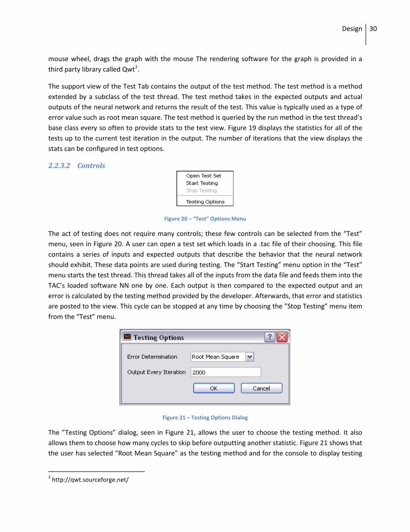
2.2.3.2 Controls
Figure 20 – “Test” Options Menu
The act of testing does not require many controls; these few controls can be selected from the “Test” menu, seen in Figure 20. A user can open a test set which loads in a .tac file of their choosing. This file contains a series of inputs and expected outputs that describe the behavior that the neural network should exhibit. These data points are used during testing. The “Start Testing” menu option in the “Test” menu starts the test thread. This thread takes all of the inputs from the data file and feeds them into the TAC’s loaded software NN one by one. Each output is then compared to the expected output and an error is calculated by the testing method provided by the developer. Afterwards, that error and statistics are posted to the view. This cycle can be stopped at any time by choosing the ”Stop Testing” menu item from the “Test” menu.
Figure 21 – Testing Options Dialog
The ”Testing Options” dialog, seen in Figure 21, allows the user to choose the testing method. It also allows them to choose how many cycles to skip before outputting another statistic. Figure 21 shows that the user has selected “Root Mean Square” as the testing method and for the console to display testing
2 http://qwt.sourceforge.net/
Design 31
information once every 2000 iterations over the test data. Testing methods are provided by a developer and are all displayed in this dialog. Remember that each neural network version has its own subclass of
ServiceLocator to provide the application with the services for that neural network. A testing method does not have to be neural network specific but it must be added to every ServiceLocator of every type of neural network that wishes to use it. This is to allow the flexibility that some versions might not wish to have certain methods and allows for the possibility that the methods can be version specific.
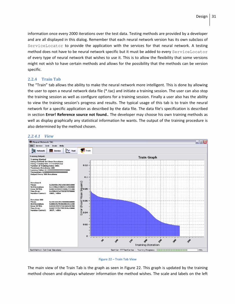
2.2.4 Train Tab The “Train” tab allows the ability to make the neural network more intelligent. This is done by allowing the user to open a neural network data file (*.tac) and initiate a training session. The user can also stop the training session as well as configure options for a training session. Finally a user also has the ability to view the training session’s progress and results. The typical usage of this tab is to train the neural network for a specific application as described by the data file. The data file’s specification is described in section Error! Reference source not found.. The developer may choose his own training methods as well as display graphically any statistical information he wants. The output of the training procedure is also determined by the method chosen.
2.2.4.1 View
Figure 22 – Train Tab View
The main view of the Train Tab is the graph as seen in Figure 22. This graph is updated by the training method chosen and displays whatever information the method wishes. The scale and labels on the left

Design 32
axis are also fully provided by the training method in question. In the case of the “Set Over Iterations” method, the graph displays the RMS of the entire neural network after each iteration of training. It should be noted that the graph expects a large number of training iterations and therefore separates the training iterations into several bins, averaging all of the content in each bin to get the data point. The x-axis is linked to however many iterations the user wishes to display. This graph’s interface also uses mouse controls to zoom and pan the graph. The rendering software for the graph is provided in a third party library called Qwt.
The support view of the Train Tab contains the output of the training method. The training method is queried by the training engine every so often to provide stats. These statistics can be anything required by the training method. The number of iterations between each output of the statistics can be configured in the “Test Options” dialog.
2.2.4.2 Controls
Figure 23 – “Train” Options Menu
Training does not require many controls as seen in the “Train” menu in Figure 23. A user can open a training set which loads in a .tac file of their choosing. This file contains a series of inputs and expected outputs that describe the behavior that the neural network should exhibit. These data points will be used when training has begun. The “Start Training” starts the training engine. The training process used
by the training engine is fully provided by the train method, which is provided by the developer. The method can post updates to the view at any time and stops when the maximum number of training iterations has been completed. However, the cycle can be stopped at any time by choosing the ”Stop Training” menu item from the “Train” menu.
Figure 24 – Training Options Dialog

Design 33
The ”Training Options” dialog, shown in Figure 24, allows the user to choose the training method. It also allows the user to choose how many cycles to skip before outputting another statistic. Also, the user can provide the total iterations he or she wishes to perform on the neural network as well as set some of the training constants such as gamma or momentum. Gamma is the learning rate constant described in section Error! Reference source not found.. Momentum is a constant in a modified weight update rule. This constant is multiplied by the last weight update used and then added to the new weight update. All this constant is used for is to help the weight’s error optimization to not become stuck in a local minimum. Figure 24 shows that the user has selected “Set Over Iterations” as the testing method and for the training statistics to be outputted to the console every 300 iterations. Testing will go on for 400 iterations and will use 0.15 as gamma and 0.0 as momentum.
The training methods are provided by a developer and are all displayed in this dialog. Remember, that each neural network version has its own subclass of ServiceLocator to provide the application with the services for that neural network. A training method does not have to be neural network specific but
it must be added to every ServiceLocator of every type of neural network that wishes to use it. This is to allow the flexibility that some versions might not wish to have certain methods and allows for the possibility that the methods can be version specific.
2.2.5 Developing for TAC This section briefly covers the steps and significant classes required to implement new neural networks
for the TAC. The TAC implements a simple plug-in architecture centered on the ServiceLocator class. Any client program that derives from the TAC can use this simple architecture to change the types of neural networks that it can support without changing any of the TAC’s core components. In fact, only a little bit of knowledge of the core components is needed in order to extend this functionality. Extendable components include the types of neural networks, testing and training methods, and finally external devices and their applications.
Client developers extend several external class components to provide this extended functionality. They
also extend ServiceLocator itself to return the extended components when asked. Each subclass
of ServiceLocator must provide a unique version id to show which type of neural network it is compatible with. This version number is used in every file and device to determine compatibility and to
identify the appropriate components. Finally, the subclass of ServiceLocator must be loaded into
ServiceLocator itself in order for the application to see the extension.

Design 34
Figure 25 - Tic Tac Toe Client Implementation
Figure 25 shows the main method of our project. This shows all that is required for the developer to do in order for the TAC to provide all of the functionality for custom neural networks. The above is all that has been required for the TAC to support our Tic Tac Toe neural network. The actual classes and methods for extending everything is documented in the following sections.
2.2.5.1 ServiceLocator The ServiceLocator class is at the heart of the simple plug-in system that the TAC implements. The first step in providing a new neural network type is to subclass the ServiceLocator. Subclassing this class involves overriding the methods that follow.
virtual NNFactory* LocateNNFactory(); virtual DeviceProvider* LocateDeviceProvider(); virtual TestProvider* LocateTestProvider(); virtual TrainerProvider* LocateTrainerProvider(); virtual int getVersion(); virtual char* toString();

Design 35
The previous methods must be overridden to locate the appropriate classes for the application when requested. If this is done then the TAC will be able to successfully integrate all of the features that a new
type of neural network has to offer. Details about the returned classes from the locator methods will follow later in this section.
The getVersion method must return the type of neural network this ServiceLocator belongs to.
All of the neural network files and data files that this ServiceLocator can handle must implement the same version number. Two different types of neural networks must not return the same version number or incompatibilities may occur.
The toString method must return an identifier string so that a human can identify if this neural network type is the type that he or she wants. Specifically, this is mostly used in the drop down box of the “New Neural Network Dialog” seen in Figure 15. Naming the type of neural network should have something to do with its use: such as “Tic-Tac-Toe” or “Battleship.”
2.2.5.2 NNFactory The NNFactory class allows the creation of a particular type of neural network. Whenever a neural network is opened it needs to be created in memory. This builds a representation of the specific type of neural network (NNApprox class) that the file version has asked for. This class is meant to be subclassed and should override the method that follows.
virtual NNApprox* build(double* weights, int length);
The previous method is the only method that’s required to be overridden. This method takes in an array of weights and the total number of weights and returns the specific type of neural network that this class builds. The type of neural network that this class builds should be the same as the
ServiceLocator it belongs to. An example for the Tic Tac Toe application follows in Figure 26.

Design 36
Figure 26 – TTTFactory.h – A subclass of NNFactory
2.2.5.3 NNApprox The NNApprox class is an abstract class that provides access to an underlying neural network. This class must be implemented by a subclass to provide a particular type of neural network. The main purpose of
this class is to break out the functionality of the underlying nn class as well as keep track of its configuration. The only method that subclasses need to override follows.
virtual void build();
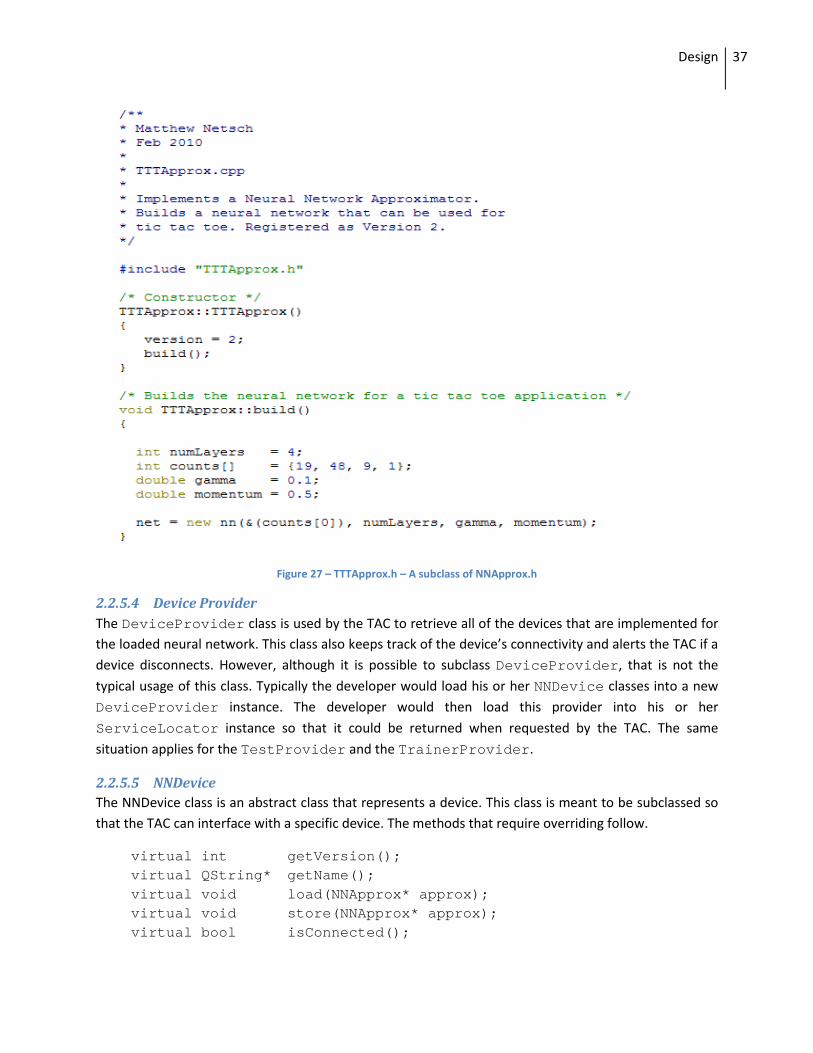
The previous method builds up the underlying neural network to the configuration that the version type that this subclass implements. The developer must also set the version member variable to the version number that this subclass implements as well. An example for the Tic Tac Toe application follows in Figure 27.
Design 37
Figure 27 – TTTApprox.h – A subclass of NNApprox.h
2.2.5.4 Device Provider The DeviceProvider class is used by the TAC to retrieve all of the devices that are implemented for the loaded neural network. This class also keeps track of the device’s connectivity and alerts the TAC if a device disconnects. However, although it is possible to subclass DeviceProvider, that is not the
typical usage of this class. Typically the developer would load his or her NNDevice classes into a new DeviceProvider instance. The developer would then load this provider into his or her
ServiceLocator instance so that it could be returned when requested by the TAC. The same
situation applies for the TestProvider and the TrainerProvider.
2.2.5.5 NNDevice The NNDevice class is an abstract class that represents a device. This class is meant to be subclassed so that the TAC can interface with a specific device. The methods that require overriding follow.
virtual int getVersion(); virtual QString* getName(); virtual void load(NNApprox* approx); virtual void store(NNApprox* approx); virtual bool isConnected();

Design 38
virtual void testConnection(); virtual void setConnected(bool connected); virtual void configure(); virtual bool isConfigurable(); virtual void reload(); virtual double evaluate(double* inputs, int numInputs); virtual void constructViews(NNDevice* device, DeviceView**
view, QWidget** controls);
• The getVersion method must return the type of neural network this NNDevice belongs to.
• The toString method must return an identifier string so that a human can identify what device this represents.
• The load method stores the weights of the device into the neural network passed into it.
• The store method stores the weights from the neural network passed into it to the device.
• The isConnected method returns the status of the connection.
• The testConnected method tries to ping the external device with a blocking behavior.
• The setConnected method sets the connection status.
• The configure method opens a configuration dialog so that a user may change the connection settings.
• The isConfigurable method returns if the device has a configuration dialog or not.
• The reload method attempts to reinitialize the connection to the external device. This is called when the device has been deemed unconnected.
• The evaluate method gives the inputs to the neural network and returns the result from the device.
• The constructViews method constructs the main view and the support view for the device so that the Device Tab may display the Device’s application.
2.2.5.6 NNTester The NNTester class is an abstract class that provides a particular testing method. The TAC uses this
method provided from the TestProvider returned from the ServiceLocator class of the loaded neural network. It takes these methods and provides for the user a set of selectable options in order to run a testing session. The methods a subclass must override in order to create a new testing method follow.
virtual double getError(double* outputs, int outLen, double expectedOutput);
virtual QString* getName(); virtual QString* getStats(); virtual QString* getScaleName(); virtual double getScaleMax();

Design 39
virtual QwtScaleDraw* getScaleDraw(); The getError method takes in the expected output and the outputs of the neural network and returns the error. The error could be whatever the testing method wishes it to be.
The getName method returns a human readable identifier so that the TAC may provide a label for this testing method.
The getStats method returns what is to be printed on the console to the left of the graph in the view. This however is only printed at every iteration that the user has specified in options.
The getScaleName method returns the label of the y-Axis for the graph.
The getScaleDraw method returns the drawing class for the labels on the y-Axis. Please see Qwt
documentation on QwtScaleDraw.
2.2.5.7 NNTrainer The NNTrainer class is an abstract class that provides a particular training method. The TAC uses this
method provided from the TrainerProvider returned from the ServiceLocator class of the loaded neural network. It takes these methods and provides for the user a set of selectable options in order to run a training session. The methods a subclass must override in order to create a new training method follow.
virtual void run(); virtual QString* getName(); virtual QString* getStats(); virtual QString* getScaleName(); virtual double getScaleMax(); virtual QwtScaleDraw* getScaleDraw();
The run method is the main method of the trainer. This method should post updates as training cycles are completed.
The getName method returns a human readable identifier so that the TAC may provide a label for this training method.
The getStats method returns what is to be printed on the console to the left of the graph in the view. This however is only printed every iteration that the user has specified in options.
The getScaleName method returns the label of the y-Axis for the graph.
The getScaleDraw method returns the drawing class for the labels on the y-Axis. Please see Qwt documentation on QwtScaleDraw.

Design 40
2.2.6 File Specifications The file specifications that the TAC uses are as follows.
2.2.6.1 Neural Network File Format of a neural network (*.nn) file:
32 bit integer which specifies the version of the neural network 32 bit integer which specifies how many weights follow 64 bit floating point numbers that specifies the weights of the neural network … ( More weights until the length is satisfied above )
The version integer effectively specifies the structure of the Neural Network, which can be used to interpret the connections that each weight is assigned to. In this way an entire neural network’s configuration can be saved and loaded, including its structure and memory.
2.2.6.2 TAC Data File Format of the TAC data (*.tac) file used in testing and training:
32 bit integer which specifies the version of the neural network 32 bit integer which specifies the number of inputs that follow 64 bit floating point numbers that specifies the inputs of the neural network … ( More inputs until the length is satisfied above )
64 bit floating point number that specifies the output corresponding to the inputs above … ( More number of inputs, inputs, and output chunks until end of file )
This file effectively stores input/output pairs which specify the correct behavior of the neural network. This allows for both testing and training the neural network using this data. The algorithms in which it does this are out of the scope of this document.
2.3 Parallel Neural Network The parallel neural network must process a set of inputs and produce an output that is the same as that of the sequential neural network algorithm. This embedded system must take advantage of neural network parallelism to produce an output more efficiently than a sequential processor. The only difference between the inputs and outputs of the parallel and sequential neural networks should be the time taken to calculate them.
2.3.1 Parallel Structure Analysis Considering a neural network consisting of multiple fully connected layers of neurons helps identify which parts of the network may be calculated in parallel. It is impossible for each of the sequential layers to calculate an output without having the entire output of its previous layer; therefore, it is impossible to take advantage of any parallelism concerning consecutive layer calculations, limiting the parallel calculation to the neurons within a layer.

Design 41
The parallelism of a layer of neurons is possible because the output of each neuron does not depend on the output of any of the other neurons in the layer. Each neuron must simply iterate over the set of outputs from the previous layer and calculate its output using the neuron output equation:
Given that each neuron in a layer has the same number of inputs, this method of parallel neuron calculations will improve the efficiency of each layer by a factor equal to the number of neurons in that layer. For example, a layer containing ten neurons, each with five inputs, must perform the neuron output equation ten times; a sequential algorithm would perform the calculations sequentially ten times—once for each neuron in the layer. Each neuron calculation requires scaling five inputs, resulting in five multiplications. The output calculation also requires summing each scaled input, resulting in four additions. The activated output must then be calculated from the final accumulated sum of scaled inputs. The result for a sequential neural network is:
In contrast, the parallel neural network performs all ten neuron calculations in parallel, giving sequential multiplications, sequential additions, and sigmoid. For this example, the number of sequential calculations is reduced by a factor of ten, which is the number of neurons in the layer.
Sequential Multiplications Sequential Additions Sequential Sigmoids
Sequential Neural Network 50 40 10 Parallel Neural Network 5 4 1
Table 1 - Sequential operations for 10 neuron layer with 5 inputs
The importance of this analysis is that by calculating each neuron’s output simultaneously, the number of neurons in a layer does not affect the number of sequential calculations for that layer. The only factor affecting the number of sequential calculations in a layer is the number of inputs from the previous layer.
2.3.2 Efficiency Having a physical device for each neuron in a neural network can result in a lot of hardware. Each neuron must minimally have its own multiplier, its own adder, and its own memory. And more hardware

Design 42
is required for calculating the sigmoid: as this contains a division and an exponential, is a costly calculation. In order to reduce the amount of hardware and decrease calculation time, all calculations will be performed using integer multipliers and adders, and the sigmoid will be calculated from a table.
Floating point addition and multiplication requires many sequential integer multiplications and additions to obtain an answer, resulting in more hardware and increased calculation time. In order to maximize
efficiency, no floating point calculations will be performed in a neuron.
2.3.3 Neuron The neuron block performs the same function as a neuron in a sequential NN. It reads in all of its inputs, scales them by the weights along their connections, sums each scaled input, and calculates the activation function from the sum, which is output to the “y_j” port. When “y_j” is set, “oe,” the output enable goes high.
Figure 28 shows the schematic symbol of the neuron; all schematic symbols show input ports on coming in from the left, and all output ports going out to the right.
Figure 28 - Neuron schematic symbol
The inputs “y_i” and “i” correspond to the and from the neuron equations. While the neuron’s chip enable, “ce,” is high, the neuron expects the index, “i,” input to start incrementing and the “y_i” input to feed in the corresponding input values for the index “i.” After all of the inputs are read, the chip enable is set to low by the layer logic controlling the neuron, the inputs are scaled by their corresponding weights, these scaled inputs are summed, and the sigmoid begins calculating its result. When the sigmoid is finished, “y_j” is set to the output value, and “oe,” the output enable, is set to high. Pulsing the “reset” input resets the neuron to its initial state.
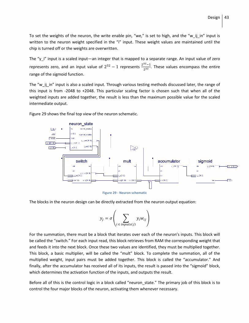
Design 43
To set the weights of the neuron, the write enable pin, “we,” is set to high, and the “w_ij_in” input is written to the neuron weight specified in the “i” input. These weight values are maintained until the chip is turned off or the weights are overwritten.
The “y_i” input is a scaled input—an integer that is mapped to a separate range. An input value of zero
represents zero, and an input value of represents . These values encompass the entire
range of the sigmoid function.
The “w_ij_in” input is also a scaled input. Through various testing methods discussed later, the range of this input is from -2048 to +2048. This particular scaling factor is chosen such that when all of the weighted inputs are added together, the result is less than the maximum possible value for the scaled intermediate output.
Figure 29 shows the final top view of the neuron schematic.
Figure 29 - Neuron schematic
The blocks in the neuron design can be directly extracted from the neuron output equation:
For the summation, there must be a block that iterates over each of the neuron’s inputs. This block will be called the “switch.” For each input read, this block retrieves from RAM the corresponding weight that and feeds it into the next block. Once these two values are identified, they must be multiplied together. This block, a basic multiplier, will be called the “mult” block. To complete the summation, all of the multiplied weight, input pairs must be added together. This block is called the “accumulator.” And finally, after the accumulator has received all of its inputs, the result is passed into the “sigmoid” block, which determines the activation function of the inputs, and outputs the result.
Before all of this is the control logic in a block called “neuron_state.” The primary job of this block is to control the four major blocks of the neuron, activating them whenever necessary.

Design 44
All of the inputs except the clock are fed directly into the control logic, which determines whether or not to pass them through to their target blocks. From there, the inputs are passed into the switch, which starts the process of retrieving weights from RAM and feeding them through the neuron. All of this data propagates through the system until the sigmoid is fired, which sets the output enable pin high and sets the output to the neuron’s output.
2.3.3.1 Neuron State
Figure 30 - Neuron state diagram
The neuron state block’s purpose is to activate and deactivate the switch and sigmoid blocks. It initially starts in the “idle” state, as seen in Figure 30, which disables both the switch and sigmoid blocks. Once the “enable” input goes high, the system transitions to the “read” state, which turns on the switch block and waits for inputs to be clocked into it. Once all of the inputs have been read, the “enable” input goes low, switching the system into the “done” state. When this switch occurs, the switch block is deactivated and the sigmoid block is activated. The system remains in this state until it receives a “reset” signal, indicating that the neuron is being fired again.

Design 45
Figure 31 - Neuron State schematic symbol
The neuron state block, seen in Figure 31, takes five inputs: clk, enable, reset, y_i_in, and i_in. The “clk” input is the common clock for the circuit; the “enable” input is the state machine input indicating if the neuron should be reading values or calculating a sigmoid; the “reset” input is the state machine input indicating that the neuron should reset all of its values and return to an idle state so that the neuron can fire again.
There are also four outputs: switch_enable, sigmoid_enable, y_i_out, and i_out. The switch enable and sigmoid enable outputs control the chip enable pins on the switch and sigmoid blocks. The “y_i_out” and “i_out” outputs filter the two inputs “y_i_in” and “i_in” so that they only pass through while the system is reading input values.
It is important that the neuron stays in the “done” state instead of immediately going back to “idle” once the sigmoid is calculated. This is because the output of the neuron must be held at the sigmoid output value until every neuron in the layer has fired. Once this happens, the logic between the layers feeds each of the neuron’s outputs into the next layer. If any of these outputs are reset before the layer logic activates, then the neural network will calculate an incorrect output.

Design 46
2.3.3.2 Switch The switch’s job is to take a sequence of inputs, look up their corresponding weights, and feed the input, weight pair into the multiplier. The schematic symbol for this block can be seen in Figure 32.
Figure 32 - Switch schematic symbol
The switch block takes six inputs: clk, ce, y_i_in, i_in, we, and w_ij_in. The “clk” input is the standard clock input, the “ce” input is the chip enable input, the “y_i_in” input is the 32 bit input value representing the output of one neuron from the previous layer, and “i_in” is an arbitrary number representing the index of the neuron from the previous layer whose output is being fed into the switch.
The last two inputs, “we” and “w_ij_in,” are the write enable inputs and weight inputs for updating the stored neuron input weights. These inputs are fed directly into a RAM block; the schematic symbol for this block can be seen in Figure 33.
Figure 33 - Weight lookup schematic symbol

Design 47
The function of this block is to read the memory at the given address if “we” is low, and to write “di” to the memory at the given address if “we” is high. It is a simple RAM module that stores up to 256 32-bit weights.
2.3.3.3 Multiplier
Figure 34 - Multiplier schematic symbol
The multiplier block, seen in Figure 34, is used for scaling the signals traveling along the connections between neurons. It performs the task of calculating , which is used in the neuron output
equation.
While the function of this block is simple, care must be taken in choosing which bits of the output to map to the next block in the system: the accumulator. A 32 bit multiplier produces a 64 bit output, and the accumulator expects a 32 bit input. In order to determine what output pins to connect to the accumulator, the normalization of the input values must be considered.
is a 32 bit input normalized between zero and one. This is the same normalization as the output of the sigmoid block, as this value may be fed directly from the previous layer of neurons, through the switch, and into the multiplier.
is a 32 bit weight normalized between -2048 and 2048. Multiplying this value with should produce
the output normalized between the same range. However, this is not the case. Instead, the scale
factors multiply, giving an actual output of:
The scaling factor for each of these terms is determined by the normalized range of the term. The entire range of is . The entire range of a 32 bit integer is . Dividing
the scaled value by the original value gives the scaling factor: . The same process can be applied to determine the scaling factors, given below, for the other terms, and .

Design 48
The output value is off by a factor of . In order to fix this scaling, the low 32 bits of the multiplier can be discarded, and the high 32 bits kept, resulting in the correctly scaled and multiplied output.
2.3.3.4 Accumulator The purpose of the accumulator, seen in Figure 34, is to sum all of the inputs to the neuron, and then to feed their sum into the sigmoid block once all of the inputs are retrieved.
Figure 35 - Accumulator schematic symbol
This block takes as an input a 32 bit word normalized between 2048 and -2048. It receives the input from the multiplier block, which scales the signals traveling along connections between neurons.
While the accumulator block performs only one simple function, the behavior of its output requires consideration of its function within the neuron block. The accumulator must supply its output to the sigmoid, but it has no idea how many inputs it must process before giving this value.
First, the accumulator must hold its output value throughout the entire calculation of the sigmoid block. The sigmoid will calculate a new output whenever the accumulator output changes.
Second, the accumulator has memory so it must be reset at some point while the neuron is firing. Two possibilities for this are to reset it after the sigmoid has finished processing or to reset it before the neuron fires. If the accumulator is reset before the neuron fires, then it can either perform its reset synchronously before the neuron starts firing, or it can perform its reset asynchronously with the assumption that the accumulator will be reset before the multiplier block finishes its first output. If the

Design 49
accumulator is reset after the neuron fires, then it must be guaranteed that the neuron is not firing a second time before the input signal propagates forward to the accumulator. In this design, the neuron operation is considered to be atomic—it cannot be split up into separate instructions—so the latter case gains speed without adding risk.
The output of the accumulator block is a 32 bit integer normalized between -2048 and 2048. This output is fed into the sigmoid block to calculate the activation function of the neuron.
2.3.3.5 Sigmoid
Figure 36 - Sigmoid schematic symbol
The sigmoid schematic symbol is shown in Figure 36. The “clk” input is the common clock, the “ce” input is the chip enable input, and the “x_j” input is the 32 bit input value received from the accumulator, normalized between -2048 and +2048. The output “y_j” is the 16 bit output value normalized between 0 and 1, and the output “oe” is the output enable pin, which indicates when the sigmoid is finished calculating its result.
2.3.3.5.1 Output mapping Storing the sigmoid function in a table reduces the calculation time to one clock cycle, but requires a significant amount of memory. In order to have a reasonable amount of precision, up to 64kb of data will be used to store the sigmoid, and the stored values will be preprocessed to ensure that the extent of the values covers only the necessary ranges of the sigmoid.
The number of accessible addresses depends on the size of the word being stored. Using 64kb of RAM allows up to 65,536 bytes to be stored and addressed, but the precision when using only 8 bits would be
. This is unacceptable, as such a large error allows only possible neuron output values; this is hardly enough precision for a neural network. Doubling the size of the
stored word to 16 bits improves the precision quite a bit, to . This
improved precision gives possible output values. This should be enough precision, as

Design 50
the error of the final system must be within of the actual negamax output value, since each possible
output is spaced by , as specified in section 1.2.3. If turns out to be too small a precision, then the
NN can be further trained such that .
The next step is to determine the mapping between sigmoid values and table values. The output of the sigmoid function is always between 0 and 1; the output of the table is always between 0 and 65535.
Figure 37 - Sigmoid graph
Quick inspection of Figure 37 shows that the sigmoid might be rotationally symmetric about the Y axis at . If this is true, then the following condition must be satisfied:
Substituting the definition of the sigmoid function results in a quick proof:
This property of the sigmoid function helps determine the lower bound of sigmoid values to be stored, as all negative values can be ignored, and the symmetry can be used.
The upper bound of the sigmoid function can be determined by inspection from Figure 37. At , the sigmoid function levels out at about 1; similarly, at , the sigmoid function levels out at zero. Since the sigmoid function is rotationally symmetric about , the lower part can be ignored, and the upper bound may be set at .
Unfortunately, the range of sixteen bit words is an exponent of two, and five is not an exponent of two. This makes conversions between normalization extremely difficult, due to the required use of a
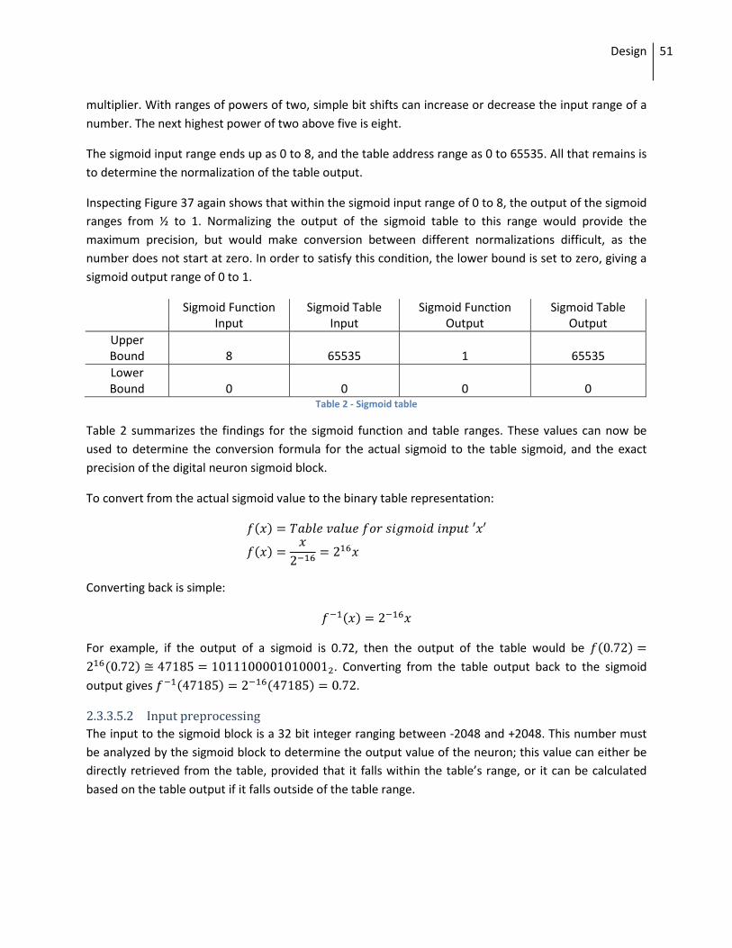
Design 51
multiplier. With ranges of powers of two, simple bit shifts can increase or decrease the input range of a number. The next highest power of two above five is eight.
The sigmoid input range ends up as 0 to 8, and the table address range as 0 to 65535. All that remains is to determine the normalization of the table output.
Inspecting Figure 37 again shows that within the sigmoid input range of 0 to 8, the output of the sigmoid ranges from ½ to 1. Normalizing the output of the sigmoid table to this range would provide the maximum precision, but would make conversion between different normalizations difficult, as the number does not start at zero. In order to satisfy this condition, the lower bound is set to zero, giving a sigmoid output range of 0 to 1.
Sigmoid Function Input
Sigmoid Table Input
Sigmoid Function Output
Sigmoid Table Output
Upper Bound 8 65535 1 65535 Lower Bound 0 0 0 0
Table 2 - Sigmoid table
Table 2 summarizes the findings for the sigmoid function and table ranges. These values can now be used to determine the conversion formula for the actual sigmoid to the table sigmoid, and the exact precision of the digital neuron sigmoid block.
To convert from the actual sigmoid value to the binary table representation:
Converting back is simple:
For example, if the output of a sigmoid is 0.72, then the output of the table would be . Converting from the table output back to the sigmoid
output gives .
2.3.3.5.2 Input preprocessing The input to the sigmoid block is a 32 bit integer ranging between -2048 and +2048. This number must be analyzed by the sigmoid block to determine the output value of the neuron; this value can either be directly retrieved from the table, provided that it falls within the table’s range, or it can be calculated based on the table output if it falls outside of the table range.

Design 52
There are four different cases that must be handled by the sigmoid block: the input less than or equal to -5, the input greater than or equal to 5, the input greater than or equal to 0 but less than 5, or the input less than 0 but greater than -5.
The first case is simple. If the input to the sigmoid block is less than or equal to negative five, then the output of the sigmoid block is simply zero. This condition and its output values are derived from Figure 37, in which the sigmoid function converges at zero for input values less than negative five.
The second case is similar. If the input to the sigmoid block is greater than or equal to five, then the output of the sigmoid block is one. This is also determined by analyzing the upper limits of Figure 37.
The third case is a simple table lookup. If the input value is between zero and five, then the relevant bits from the input value can be fed into lookup table and the output value directly passed into the sigmoid block output. The bits relevant to the address are dependent on the normalization of the input word. In this case, the input word is normalized to the values -2048 and 2048. The range of these numbers is
. The number the sigmoid is expecting is only three bits, , so the most significant 9 bits of the input value must be stripped off. Next, the input table only accepts 16 bit values, which cuts off seven least significant bits from the input value. The resulting number is a 16 bit address normalized between 0 and 8, which can be fed directly into the lookup table to produce the sigmoid output.
The last case involves preprocessing, a table lookup and some post-processing. In the case where the input value is negative and greater than negative five, the address cannot be directly fed into the lookup table. First, it must be negated so that it falls within zero to five. After performing the table lookup, the output value must again be processed such that it corresponds to the negative half of the sigmoid and not the positive half. In order to do this, the output value of the table is subtracted from the number
one. This flips the output value along , giving the correct output for the negative half of the
sigmoid.
The sigmoid block produces the final output of the neuron. It receives its inputs from accumulator, which receives its inputs from the switch. All of these blocks are controlled by the neuron_state block, which filters the input and toggles the chip enable pins as necessary to provide a correct neuron output.
2.4 Hardware and Software Driver The drivers for connecting to an external hardware neural network device were originally designed and implemented for a Xilinx Spartan 3E FPGA3 on the Diligent Nexys 2 Board4
3 http://www.xilinx.com/support/documentation/spartan-3e_user_guides.htm
. The actual neural network was later designed for the Xilinx Vertex 6 DSP FPGA. After the drivers were developed, limitations were discovered in the Spartan 3E FPGA. The FPGA did not contain enough block RAM, block multipliers, and flip-flop registers to be able to support our design for the Tic-Tac-Toe neural network. Therefore, we designed for a piece of hardware that could handle all of the necessary components. The hardware
4 http://www.digilentinc.com/Products/Detail.cfm?Prod=NEXYS2

Design 53
driver was not ported over to the device because the designs should be logically equivalent. We did not have access to a Virtex 6 FPGA so there would have been no benefit in the port.
The drivers are broken into several layers, as seen in Figure 38. The software and hardware drivers allow the connect components to encode and decode messages sent across the connection. The transfer of this information is like the connection between a client and a server. The software application which is like the client and the hardware NN is like the server. The high level requests and responses sent between the two are broken down into a message protocol, like HTTP. In order to transmit the messages; they must first be broken down into the connection protocol which can be thought of as TCP. The connection protocol is further broken down into stateless register transfer, like IP.
Figure 38 – Driver Generalization
2.4.1 Software Driver The software driver is built upon Diligent’s dynamic library that opens up the USB port to the four emulated parallel port functions. These functions are described in section Error! Reference source not found.. The responsibilities of this driver are to break apart the messages it received from the software application and implement the client part of the connection protocol. The software driver then relays the responses from the server to the requested callback.

Design 54
Figure 39 – Software Neural Network Driver
The typical inputs to send a message includes a pointer to a data buffer, an enumerated type that specifies the type of message, and an integer that specifies the length of the message as seen in Figure 39. The software driver interfaces with Diligent’s library to break down the messages from the application into chunks. These chunks are then written to the appropriate registers in the hardware driver. When the software driver receives a response from the hardware driver, it accumulates the message chunks until all of the messages are received. The software driver then sends the received messages to the callback function that the software application provided. It should be noted that other drivers can interface with the library in order to provide different types of neural network providers.
2.4.2 Hardware Driver The hardware driver for the project is made for the Diligent Nexys 2 development board. Some of the features of the board consist of the Xilinx Spartan 3E FPGA and a USB interface. The USB interface on the board side is connected to several ports which provide access to an emulated parallel data port. This consists of up to 256 addressable registers each 8 bits wide. There are other control lines such as the wait line, the write line, the address strobe, and the data strobe. Four functions are defined to communicate over this connection. They include: read address register, write address register, read data register, and write data register. Exact documentation on the signals of this interface is available on the

Design 55
Diligent website5
. Several components make up the hardware driver in order to handle the messages and the connection protocol.
Figure 40 – Hardware Driver
2.4.2.1 Switch The Switch component contains an array of 256 flip flops in order to store the 32 8bit connection registers. Only 32 were selected so that the message for sending propagate messages would be accomplished in one chunk. This will allow for better performance when running the neural network while keeping the size of the flip-flops down. The Switch contains a state machine to handle the four functions that the Diligent interface requires. This allows the client to read and write any registers it wants in accordance with the connection protocol. The Switch also contains logic to interface with the individual message controllers seen in Figure 39. This allows the Switch to be decoupled from the handling of specific message types. This also allows the message controllers to be decoupled from the connection protocol. The control bits between the Switch and the message controllers include write enable, write ready, write done, read enable, read ready, and read done. Their data ports include message length in and out, message data in and out, and message type in and out. The message type directly controls the enable bits of the appropriate message controller.
5 http://www.digilentinc.com/Data/Products/ADEPT/DpimRef%20programmers%20manual.pdf

Design 56
2.4.2.2 Message Controllers Each message has its own message controller. Each controller contains the state machines required to handle the reception of its message as well as provide a response. They contain all of the ports required to interface with the switch as well as the neural network. They may also contain other items as well including counters and registers to aid in their function. The outlines of the functionality are provided below and should be straight forward.
Version Controller: This controller contains no ports to interface with the neural network. Its response is simple as all it does is to reply with a 32bit value that specifies its version. The network we have developed for this board is version 2. Weights Controller: This controller contains all of the flip-flops required to store all 1353 16bit weight values for the hardware neural network. It also opens up a parallel access port to the neural network so that multiple components can read and write any of the weights they choose to. This controller of course contains the logic required to set and retrieve the weights in a series of messages to and from the switch. Counters and buffers are included in order to aid this process. Input Controller: This controller is logically very similar to the weights controller in every way. The only difference is that the weights controller does not have to decode the set message from the switch. This added functionality only adds extra states as well as an extra counter to the input controller. However, the input controller still opens up parallel access so that the input layers of the hardware neural network can read the input values. Output Controller: This controller is logically similar to the version controller in that it only accepts a blank message and sends back a simple response. The only difference is that it allows the hardware neural network to change the output register with its result. Forward Propagate Controller: This controller is logically very simple. This controller can instruct the neural network to forward propagate. The hardware neural network can notify the controller when the cycle has been completed. The forward propagate controller can also instruct the output controller to send an output message back to the client after the hardware neural network has notified completion.
2.4.3 Message Types There are 5 different message types that allow the transmission of data between the hardware neural network and the software application using it. The message types allow the neural network device to be able to set inputs, read output, initiate a forward propagate, set and retrieve weights, and query the type of neural network it is. Messages can be related to packets in a connection between a client and a server. Sometimes messages cannot fit all of its data within the 32 byte buffer limit. In this case, the message is sent in chunks.

Design 57
Using a message-based, communication system allows data to be disambiguated from each other as well as allow for modular controllers to be able to deal with messages themselves. Extending or changing the way the software application and hardware neural network communicates only involves changing the specific message controller.
2.4.3.1 Version Message Type Code: 1 ( Type Register: 00000001)
This message is sent by the client with an empty data body. When the server receives this it will form another version message and send it back with a 32-bit integer value as the data. This value contains the version that the server is using. The client can use this version value to determine if it can recognize the server’s configuration. A neural network can be configured in many ways for different applications and so it would be good if the client knew which configuration it was using. All data passed in the messages are done most significant byte first, as seen in Figure 41.
Figure 41 - Version Message
2.4.3.2 Weights Message Type Code: 2 (Type Register: 00000010)
The purpose of the weights message is to let the client set and get the hardware neural network’s weights. This is so that the software application can test, train, and save a neural network on a computer. The software application can feed the hardware neural network weights when it requires the hardware neural network to run. Both getting and setting the weights uses the same message type.

Design 58
Figure 42 – Weights Message
If the weights message is sent with an empty body it means the server will send a weights response with the body filled with all of the weights of its neural network. The order and number of weights sent back depends on the version type of the network; therefore this is one of many reasons why both the client and the server should be aware of and compatible in their versions. Each weight is a 16bit value as seen in Figure 42. Successive message chunks are sent until all of the weights have been sent back to the client.
If the request has a body it means the server will set the weight values of the hardware neural network to the ones inside the message body. The response is just an empty weights message to confirm that it’s finished setting its weights. Again the number and order of weights depends on the version of the neural network.
2.4.3.3 Inputs Message Type Code: 4 (Type Register: 00000100)
The purpose of the inputs message is to allow the software application to set and get the current inputs to the hardware neural network. These inputs are stored in the input controller and are used to feed to the hardware neural network every time a forward propagate message is sent. Not including inputs with the forward propagate message allows the software application to run the neural network with the same inputs many times in a row. Originally, this was meant to help with performance when back-propagating. Getting and setting the inputs are done with the same message type.
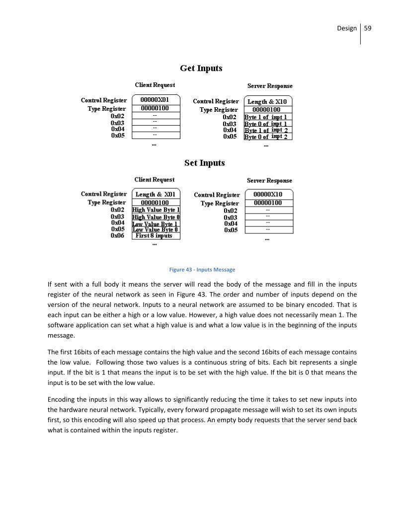
Design 59
Figure 43 - Inputs Message
If sent with a full body it means the server will read the body of the message and fill in the inputs register of the neural network as seen in Figure 43. The order and number of inputs depend on the version of the neural network. Inputs to a neural network are assumed to be binary encoded. That is each input can be either a high or a low value. However, a high value does not necessarily mean 1. The software application can set what a high value is and what a low value is in the beginning of the inputs message.
The first 16bits of each message contains the high value and the second 16bits of each message contains the low value. Following those two values is a continuous string of bits. Each bit represents a single input. If the bit is 1 that means the input is to be set with the high value. If the bit is 0 that means the input is to be set with the low value.
Encoding the inputs in this way allows to significantly reducing the time it takes to set new inputs into the hardware neural network. Typically, every forward propagate message will wish to set its own inputs first, so this encoding will also speed up that process. An empty body requests that the server send back what is contained within the inputs register.

Design 60
2.4.3.4 Outputs Message Type Code: 8 (Type Register: 00001000)
This message is sent by the client with an empty body. The server then sends back an outputs message with the contents of the output register. The register is a 16bit value and contains the result from the last time the neural network forward propagated. This message, seen in Figure 44, is sent back automatically after a forward propagate request.
Figure 44- Outputs Message
2.4.3.5 Forward Propagate Message Type Code: 16 (Type Register: 00010000)
This message is sent by the client with an empty body. The server then initializes its neural network to forward propagate. The contents of the input register are feed to the input neurons of the hardware neural network. The values are propagated through and finally the output register gets updated with the result then sends an Outputs message, seen in Figure 45, as a response with the contents of the output register.
Figure 45 – Forward Propagate Message

Design 61
2.4.4 Connection Protocol The connection protocol is used to transfer messages between the software application and the hardware neural network. Messages must be broken down into the connection protocol for them to be sent over the emulated parallel port. This protocol can be thought of like TCP transferring HTTP messages.
Figure 46– Connection State Machine
The connection protocol shown in Figure 46 is based upon a request and response scheme where the device utilizing the neural network is the client and the neural network provider is the server. The start of the connection cycle occurs when the state bits of the hardware control register is 00. Exact specifics about how this connection is made physically to the server are the duty of the adapter for the driver library. This section remains device independent and describes the connection states.

Design 62
2.4.4.1 Read Ready State Code: 00
This state occurs when no connection cycle has started and when the server has finished processing the last message sent by the client. In this state the client may modify any of the type and data registers. Then it must fill in the length bits of the control register and finally set the state bits of the control register to 01, which signifies that data is ready to be read by the server. If the client has no more data to send to the server then it can set the state to 11 signifying that it requests the server’s response and it is ready to receive information. Note that information may not be passed if the state is set to 11 and will be ignored by the server.
2.4.4.2 Read State State Code: 01
This state occurs when the client has filled in the rest of the registers with valid data and has told the server to begin reading the information. The server will then process the information for as long as it pleases. The client may not change any of the registers until the server sets the state back to 00, which signifies it is done processing the data. The client may then send the next chunk of its message if the entire message could not have fit within the 32 byte register buffer.
2.4.4.3 Write State State Code: 11
This state occurs when the client requests the response of the server. In this state the server may modify any of the registers as it pleases. When it is finished writing its message then it sets the code to 10, which tells the client to read the message from the registers. If the server has no more data to send it sets the code back to 00, which passes control back to the client.
2.4.4.4 Write Ready State Code: 10
The state occurs when the server has finished sending data and told the client to read it. The server may not change any of the registers in this state. When the client finishes reading it will set the state back to 11, which tells the server that it is ready to receive the next chunk of its message.
2.4.5 Registers The drivers are designed to allow communication between a software application and a hardware neural network through a series of messages. The messages are broken down into the connection protocol. The broken down messages are sent over USB through the emulated parallel port (EPP) used by Diligent. The EPP consists of a set of 32 registers of length 1 byte each. The control register contains the connection state as well as length of the message’s data. The type register specifies which type of message the data applies to. The data registers contain the message body. These registers can be seen in Figure 47.

Design 63
Figure 47 – Connection Registers
2.4.5.1 Control Register The control register, seen in Figure 48, contains the connection state as well as the length of the message body. Since there are 30 bytes of connection registers that can be used for each message chunk, there must be 5 bits that contain the message length. These occupy the high 5 bits of the control register. The low two bits are required to contain the state of the connection. The low bit indicates if data is ready when it is set to 1. The direction bit indicates what is doing the writing. This bit is set to 0 when the software application is writing to the hardware neural network and 1 when the other is true. This process is explained more in the connection cycle section.
Figure 48 – Control Register
2.4.5.2 Type Register The type register, seen in Figure 49, contains the message type that the data in the message body applies to. This register can be changed in the middle of a connection cycle which signifies that the writer is sending a new message of that type. This allows the writer to send multiple messages of different types within the same connection cycle. The message type is encoded using “1 hot” encoding:

Design 64
that is, every bit specifies its own message type. It is invalid for more than 1 bit to be selected at the same time. More about the process is explained in the connection cycle section and more about each message type is described in their sections.
Figure 49 – Type Register
2.4.5.3 Data Register The data registers contain the bytes of the message body and are interpreted based upon what message type they belong to. The appropriate message controller is required to decode and encode its message.
2.4.6 Driver Tester Interface This application is used to test the driver in order to determine if it is functional. A user may send and receive any message you wish to the connected device. The correct behaviors of the messages are defined in the Driver Documentation. The connected device is a Diligent Nexys 2 FPGA board pre-loaded with the driver.bit file included in this project. The .bit file is a compiled hardware configuration that can be loaded onto the FPGA. The user must pre-load the .bit file to initialize the FPGA’s configuration using Diligent’s Adept software available on their website6
6
.
http://www.digilentinc.com/

Design 65
2.4.6.1 System Diagram
Figure 50 – System Diagram
The system diagram shown in Figure 50 is the general structure of how the driver tester works. This user interface is not meant to be complicated as its only functionality is to test the driver. A user may send whatever messages he or she wishes to the hardware neural network. The user may also see the output from the hardware neural network to make sure that everything is working with the connection.
The user interface is the Dialog class which handles all of the user inputs and outputs. This dialog parses the input console and compiles a message for the software driver. The nnDriver class is the software driver and is built upon Diligent’s libraries to communicate with the hardware neural network. The software driver implements the connection protocol for both sending and receiving messages. When the software driver receives a message from the hardware neural network it notifies Dialog.
Dialog then displays the message to the user.

Design 66
2.4.6.1 Interface Example
Figure 51 – Example User – Set Inputs Message
Figure 51 shows an example use of the Input message. The software driver is connected to the hardware neural network device”AutoDOnbUsb1”. It should be noted that this is the driver name is returned from Diligent’s libraries and the interface does not choose the name. Configure opens up Diligent’s device dialog which allows the user to change the connected device.
The combo box in the Options group box allows the user to change the type of message he or she wishes to send. When the user clicks on the send button, the text in the input console is parsed and formed into a message with the type from the combo box. This message is sent to the software driver. The response message received from the software driver is shown in the output console.

Design 67
2.4.6.2 Device Group Box
Figure 52 – Device Group Box
The device group box, seen in Figure 52, contains information as to which device is connected and a button that allows you to select which device you wish to use. When the configure button is pressed, the Diligent Library’s configure dialog is displayed. Please see Diligent’s documentation for more information about its libraries.
2.4.6.3 I/O Group Box
Figure 53 – I/O Group Box
The I/O group box, seen in Figure 53, contains two text areas. The input text area allows a user to set the message body that her or she wishes a sent message to have when they click on the send button. Whitespace and characters that are not a 1 or a 0 are ignored when the message is formed before it is sent. Bytes of data are put together from the input text area to form the message body when a message is sent to the connected device. The input area is used each time when message is sent even if the same data is present from a previous message.
The output text area echoes the sent message in order to ensure the user that the appropriate message was sent. After the connected device posts its response, the dialog will display the response message. After which the user may initiate another message. Please note that the output area cannot be edited and that it clears before sending each message. Again please refer to the Driver Documentation in section Error! Reference source not found. for the correct format of messages and their responses.

Design 68
2.4.6.4 Options Group Box
Figure 54 – Options Group Box
The options group box, seen in Figure 54, allows you to select the message type you wish to send to the connected device. You may initiate a send operation when you click on the button. When this happens, a message will be sent with the type from the Message Type box and with the data parsed from the Input text area. You will not be able to send another message until the device issues its response. For more information on the types of messages and their function please refer to the Driver Documentation in section Error! Reference source not found..

4BAnalysis
69
3 Analysis
3.1 Hardware Neural Network The accuracy, precision and efficiency of each module within the hardware neural network. The neuron_state, the switch, the accumulator, and the sigmoid must be analyzed to satisfy the project goals. Accuracy analysis is necessary to verify that each component is working correctly, and that the combined embedded neural network is producing the same output as the computer neural network. Precision analysis is necessary because, since the methods used to produce the result are different, the outputs of the hardware and software networks will slightly deviate from each other—ideally by a negligible amount. Lastly, efficiency analysis must be done to ensure that the efficiency requirements of the project are being met: that the simple components are using as few clock cycles as possible and that the parallelism is beneficial.
Whereas the design was performed top down, the analysis is performed bottom up. Each component will be analyzed from its most basic module upwards in order to ensure that any problems arising are a result of the current module, and not from one of its inner child modules. It is also helpful to know the efficiency of child modules, so that the entire efficiency of the system can be calculated by combining the efficiencies of its inner modules.
This section analysis starts with the control logic for the embedded neural network: the neuron state.
3.1.1 Neuron State The neuron state module’s job is to control the activation of the switch and sigmoid blocks in the neuron. It is designed as a simple Moore machine7
Each correct state transition must be verified to determine if the neuron state module is accurately determining next states. Likewise, every input value not resulting in a state transition must also be analyzed to ensure that the state machine is not switching states incorrectly.
with four outputs, two of which represent the activation of each output module, and the other two which are two inputs—the index and the previous layer neuron output—passed through to the switch block. This unit is directly connected to all of the neuron inputs, and routes them to their correct locations.
The state transition diagram, seen in Figure 30, starts in the idle state. The first test waveform output verifies that the system correctly transitions from Idle to Read and back to Idle.
7 A Moore state machine is a finite state machine where its outputs are only dependent on the current state of the machine and not also on the inputs that lead to the current state.

4BAnalysis
70
clock cycle enable reset y_i_in i_in switch_enable sigmoid_enable y_i_out i_out 1 0 1 0 0 0 0 0 0 2 1 0 3 0 1 0 3 0 3 0 1 0 0 0 0 0 0
Table 3 - Neuron state tabulated waveform
The waveform outputs tabulated in Table 3 show that when the neuron state is “idle” and the enable pin goes high, the state machine transitions to the “read” state. The “reset” input is then set to high and the “enable” input to low, and the state machine transitions back to the “idle” state. The same process is repeated to ensure that the state machine can correctly transition multiple times.
The next test runs through all of the states—“idle” to “read” to “done” to “idle.” The input transitions for this path through the state machine are: “enable” high, then “enable” low, then “reset” high.
clock cycle enable reset y_i_in i_in switch_enable sigmoid_enable y_i_out i_out 1 0 1 0 0 0 0 0 0 2 1 0 3 0 1 0 3 0 3 0 0 0 0 0 1 0 0 4 0 0 0 0 0 1 0 0 5 0 1 0 0 0 0 0 0
Table 4 - Second neuron state tabulated waveform
The waveform outputs tabulated in Table 4 show the state machine going through the states: “idle” to “read” to “done” to “idle.” This is exactly the expected output.
Given that this state machine has so few states and inputs, further testing is not required. The output is accurate, precise and efficient for all states and inputs.
3.1.2 Switch The switch module has two primary functions: to lookup weights corresponding to an index, and to store weights corresponding to an index. If the write enable pin, “we,” is high, then the input in “w_ij_in” should be stored for the index “i_in.” If the write enable pin is low, then the output “w_ij” should contain the stored weight for the index “i_in.”
All of the memory management for the switch module is handled in the ram_weight child module. Before verifying that the switch works correctly, first the ram_weight module must be verified.
The inputs of the ram_weight module are standard: clk, ce, we, di, and do. Both reading and writing must be tested; it is simple to test them in a single test bench. First, three weights will be saved. The first will be stored at index zero and will contain the hexadecimal value “01010101.” The second will be stored at index 128 and will contain the hexadecimal value “80808080.” The third and last will be stored

4BAnalysis
71
at index 255 and will contain the hexadecimal value “FFFFFFFF.” After saving each of these values, which should take three clock cycles, the “we” pin will be set to low and the three values will be read back.
The reason for choosing the indices 0, 128, and 255 is to verify that there are 256 elements in the RAM module, and that values can be stored at the extremities of the memory.
clock cycle we ce addr di do 1 1 0 0x01010101 0x01010101 2 1 128 0x80808080 0x80808080 3 1 255 0xFFFFFFFF 0xFFFFFFFF 4 0 0 0 0x01010101 5 0 128 0 0x80808080 6 0 255 0 0xFFFFFFFF
Table 5 - Ram weight test waveform
Table 5, the output waveform for the ram_weight test, shows that the ram_weight module correctly saved and loaded three values in six clock cycles. This is all that is required for the module to serve its purpose in its parent module, the switch.
Now that the ram_weight module is verified, the same test can be applied to the switch. The only difference should be that the output includes the corresponding input to the block.
clock cycle ce y_i_in i_in we w_ij_in oe y_i_out w_ij 1 1 1 0 1 0x01010101 1 1 0x01010101 2 1 2 128 1 0x80808080 1 2 0x80808080 3 1 3 255 1 0xFFFFFFFF 1 3 0xFFFFFFFF 4 1 1 0 0 0 1 1 0x01010101 5 1 2 128 0 0 1 2 0x80808080 6 1 3 255 0 0 1 3 0xFFFFFFFF
Table 6 - Switch test waveform
Just as before, the weights were correctly stored and retrieved. This time, however, the inputs were correctly passed through the switch module to its output, verifying that the switch’s outputs are accurate. Since the entire process took six clock cycles, it is also as efficient as needed.
3.1.3 Multiplier The multiplier block consists of a 32 bit signed multiplier. It should return all results in one clock cycle, and should be able to multiply any combination of negative and positive integers to the extent of their range.

4BAnalysis
72

4BAnalysis
73
Table 3 contains the multiplications to be tested, including multiplication by zero, multiplication of end points, and a few small multiplications for quick verification.
y_i w_ij x_ij 2 3 6
-4 -10 40 -2147483648 2147483647 -4611686016279900000 2147483647 2147483647 4611686014132420000
-2147483648 -2147483648 4611686018427390000 2147483647 -2147483648 -4611686016279900000
0 100 0 100 0 0
Table 7 - Multiplication input/output values
The multiplier waveform is too large to put into this report, but the final output of the system directly matches the data in Table 7, with one clock cycle for each calculation. In six clock cycles, the multiplier correctly output the six values in Table 7. This test verified that the multiplier accurately produced the 64 bit output of a 32 bit multiplier for all of its extreme cases and for a few intermediate cases.
3.1.4 Accumulator The accumulator block takes its input from the multiplier and, if chip enable is high, accumulates the values into the output register. Regardless of whether or not the chip is enabled, reset will clear the output register and set it to zero.
Negative numbers are valid inputs to the accumulator. If a negative number is received, it should subtract it from the stored accumulated value. This is the main reason for having a -2048 to 2048 range for the 32 bit values coming in and out of the accumulator. It is highly unlikely for a scaled output to be even close to 2048, given a previous layer of 256 neurons, which is limited by the bit size of the index being passed through the system. For the accumulator value to exceed 2048 or -2048, all of the outputs of the previous layer must be equal to one, and all of the weights must be greater than eight or less than negative eight. Most of the weights from the trained Tic-Tac-Toe network were significantly closer to zero, ranging between about -12 and +12.
The accumulator design, however, does not need to take this normalization into account; it merely adds 32 bit binary numbers and keeps track of the result. Table 8 shows the tabulated output waveform of the accumulator after three single increments, two double increments, and a triple increment, followed by a reset.
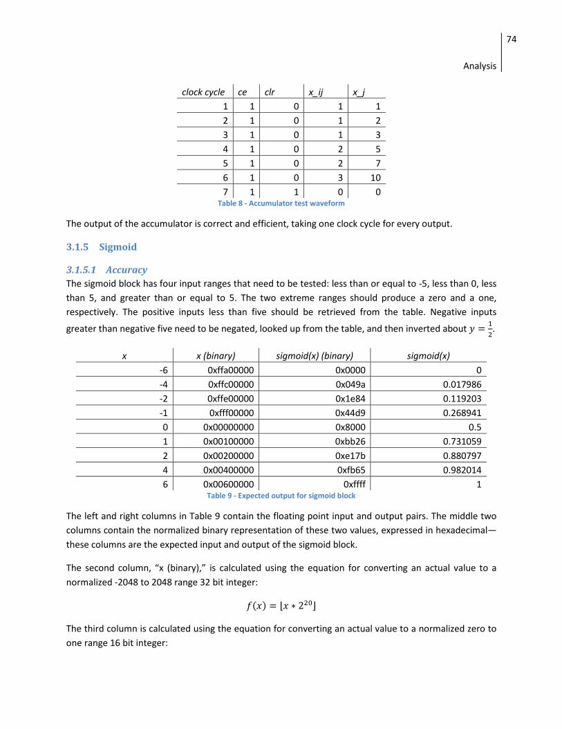
4BAnalysis
74
clock cycle ce clr x_ij x_j 1 1 0 1 1 2 1 0 1 2 3 1 0 1 3 4 1 0 2 5 5 1 0 2 7 6 1 0 3 10 7 1 1 0 0
Table 8 - Accumulator test waveform
The output of the accumulator is correct and efficient, taking one clock cycle for every output.
3.1.5 Sigmoid
3.1.5.1 Accuracy The sigmoid block has four input ranges that need to be tested: less than or equal to -5, less than 0, less than 5, and greater than or equal to 5. The two extreme ranges should produce a zero and a one, respectively. The positive inputs less than five should be retrieved from the table. Negative inputs
greater than negative five need to be negated, looked up from the table, and then inverted about .
x x (binary) sigmoid(x) (binary) sigmoid(x) -6 0xffa00000 0x0000 0 -4 0xffc00000 0x049a 0.017986 -2 0xffe00000 0x1e84 0.119203 -1 0xfff00000 0x44d9 0.268941 0 0x00000000 0x8000 0.5 1 0x00100000 0xbb26 0.731059 2 0x00200000 0xe17b 0.880797 4 0x00400000 0xfb65 0.982014 6 0x00600000 0xffff 1
Table 9 - Expected output for sigmoid block
The left and right columns in Table 9 contain the floating point input and output pairs. The middle two columns contain the normalized binary representation of these two values, expressed in hexadecimal—these columns are the expected input and output of the sigmoid block.
The second column, “x (binary),” is calculated using the equation for converting an actual value to a normalized -2048 to 2048 range 32 bit integer:
The third column is calculated using the equation for converting an actual value to a normalized zero to one range 16 bit integer:

4BAnalysis
75
Figure 55 shows the graphed output of the sigmoid, using the data from the “sigmoid(x)” column in Table 9; it correctly shows a sigmoid function.
Figure 55 – Sigmoid block output graph
The output of the hardware sigmoid waveform exactly matches the expected output from Table 9, using four clock cycles per calculated output. This table includes values in all four input ranges for the sigmoid, indicating that the sigmoid correctly produces an output for each of its four possible input ranges.
The sigmoid takes four clock cycles to produce its output. Each of the four blocks before it—the neuron_state, the switch, the multiplier, and the accumulator—take one clock cycle to complete. Summing these numbers gives the total number of clock cycles gives 4*1+4 = 8 clock cycles for a neuron to completely calculate its result.
3.1.5.2 Precision The precision of the sigmoid output is due to the quantization error of both its input and its output. This error varies for each point on the sigmoid, so in order to obtain useful information about the error, it must be calculated and analyzed using statistical methods. For the purposes of this project, a mean and standard deviation will suffice.
Quantization error comes from the rounding of inputs and outputs. To demonstrate this concept, consider a smaller example of a function that squares its input, and accepts 4 bit integers representing values between zero and one as inputs, and outputs a 4 bit number of the same range. The graph of this function is represented in Figure 56.
0
0.2
0.4
0.6
0.8
1
1.2
-10 -5 0 5 10
y
x
sigmoid(x)
sigmoid(x)

4BAnalysis
76
Figure 56 – Square Function
The green line represents the quantized output function; the blue line represents the actual output function. It is quite apparent that the error between the two functions is significant—the slight bend at X=0.5 is inaccurate, and is due to the plotting library. A graph of the error—the absolute value of the difference between the quantized functions—can be seen in Figure 57.
Figure 57 – Square function quantization error
In this example, the maximum error is about 0.15. This is unacceptable for the neural network, as the error spans a great portion of the output range of zero to one. In order to decrease the error, the output
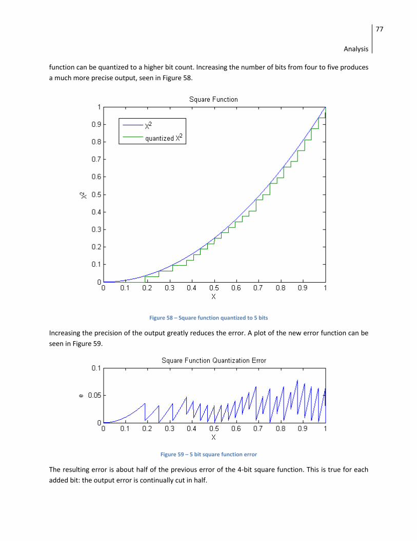
4BAnalysis
77
function can be quantized to a higher bit count. Increasing the number of bits from four to five produces a much more precise output, seen in Figure 58.
Figure 58 – Square function quantized to 5 bits
Increasing the precision of the output greatly reduces the error. A plot of the new error function can be seen in Figure 59.
Figure 59 – 5 bit square function error
The resulting error is about half of the previous error of the 4-bit square function. This is true for each added bit: the output error is continually cut in half.

4BAnalysis
78
Applying the same quantization to the sigmoid function produces the quantized sigmoid seen in Figure 60.
Figure 60 – Quantized sigmoid output
There doesn’t seem to be any visible difference between the actual sigmoid and the quantized sigmoid. There is a difference, but it’s too small to be seen given the domain and range of this graph. Figure 61, a plot of the error function of this sigmoid, gives a better picture.

4BAnalysis
79
Mean STD Max 1.96E-05 1.43E-05 7.61E-05
Figure 61-- Sigmoid quantization error
The most important aspect of this sigmoid quantization error function is the maximum error. Assuming that the sigmoid is the dominant error in the system, then an error of 7.61E-05 is acceptable provided that the network is trained with this error taken into account. Given that the Tic-Tac-Toe network for
the project has only three outputs, each of which are spaced by , the maximum acceptable error for the
network is . 7.61E-05 is significantly less than ; this error suffices.
In order to prove that the sigmoid is the dominant error in the system, the combined error of the neuron_state, switch, mult, and accumulator blocks must be determined.
The error of the neuron_state is simply the error of , which is equal to the rounding error of the input. The maximum rounding error for the 32 bit zero-to-one normalized input is
. The switch introduces a new input, , which is a normalized 32 bit integer ranging from -2048
to 2048—the error for the weight is equal to the rounding error, or . Both of these numbers are fed into the multiplier.

4BAnalysis
80
Multiplication of values with errors requires a small amount of calculation to determine the resultant error:
Assuming that and are their maximum values, the maximum error reduces to:
Feeding this error into the accumulator causes the error to add. The maximum number of nodes in any layer of the network is 48, giving a maximum error of: . This error is less than the maximum input error of the sigmoid block, which is determined by dividing the range of the inputs divided by the range of the scaled inputs. This error is the quantization error of the sigmoid input, which turns out to be:
This means that the actual error of the input signal to the sigmoid block is less than the maximum error calculated earlier, in all cases. Because of this, the sigmoid is the dominant error in the system, and its error merely adds with each subsequent layer. In the Tic-Tac-Toe network, there are three layers
calculating sigmoids, giving a final absolute error of . This
final error is an indication of how precise the hardware Tic-Tac-Toe NN’s output is with respect to its software counterpart. The resultant error of is the maximum value by which the two answers can differ. An error this large may be significant for a neural network fitting a continuous function—that is, the expected output values are continuous across the entire zero to one range. It is
not significant for the Tic-Tac-Toe application, as the expected outputs are separated by intervals of , as
determined in section 1.2.3. If the distance between expected outputs is more than twice as great as the maximum output error, then the system will produce correct results for all input values. This satisfies the requirement that the parallel hardware NN produce the same output result as its software equivalent.

4BAnalysis
81
3.1.5.3 Efficiency The hardware NN must produce the same output as a software NN with the equivalent structure, and it must produce this output more efficiently. For this project, efficiency will be measured by comparing the time for each NN to produce its output. An effective way to measure time is by figuring out how many clock cycles are used for each NN to produce its result.
One clock cycle takes a fixed amount of time, depending on the clock speed of its processor. For the time calculations in this section, all processors are assumed to have a 3 GHz clock speed, which is 3,000,000,000 clock cycles per second, or 333 nanoseconds per clock cycle. Multiplying the time per clock cycle by the number of clock cycles required to complete a calculation gives the total time required to complete the calculation.
The hardware neural network takes 100 clock cycles to complete its output. This number can be determined analytically by figuring out how many clock cycles are required to calculate the outputs for a single layer of neurons.
The two constants used—the number of clock cycles per input, and the number of clock cycles per neuron—were determined in section 3.1.1 and 3.1.4.
Applying this to the complete network gives a total number of clock cycles of:
Given that each clock cycle takes 333 ns, the total time taken on a 3 GHz processor to complete the entire output calculation for the hardware neural network is:
For the sequential NN implementation, assume that the processor running the NN is dedicating each clock cycle to NN calculations. On a real machine, the NN processing would be prioritized with the other applications running, making it take more clock cycles to complete. Also assume that the number of clock cycles to calculate the output of a neuron is the same. This results in the total number of clock cycles:

4BAnalysis
82
Converting this to seconds gives:
The time taken to process the sequential NN is slightly more than an order of magnitude greater than that of the hardware NN. The benefit is even greater for larger networks.
Scale Parallel NN Sequential NN 1 127 1969 2 222 6010 3 317 12739 4 412 22156 5 507 34261 6 602 49054 7 697 66535 8 792 86704 9 887 109561
10 982 135106
Table 10 - Clock cycles required to process neural network
The right two columns of Table 10 show the number of clock cycles required for both the parallel and the sequential neural networks to complete the calculation of a neural network. The left column, the scale, specifies how many nodes are in each layer of the network in relation to the number of nodes in each layer of the original network. This indicates that the parallel hardware design is significantly more efficient than its software equivalent.

4BAnalysis
83
Figure 62 - Parallel vs. Sequential Time Requirements
Figure 62 shows how parallel and sequential neural networks compare over a very large complexity range. Complexity 1 on the x-axis is the Tic-Tac-Toe neural network. The neural network at each complexity value is determined as follows: the number of input nodes is multiplied by the complexity value; hidden layer 1 always has 2.5 times the number of input nodes; hidden layer 2 always has half of the number of input nodes, and the output layer always has 1 node. A as complexity increases, the time required for a sequential neural network increases exponentially as seen in the figure. At complexity level 100, the sequential neural network takes about 4 seconds to complete and the parallel neural network takes about 4 milliseconds.
4 Conclusion The two main goals of the project were to implement an embedded, parallel neural network that improves upon the efficiency of traditional neural network algorithm implementations, and also to verify that this network worked correctly for a real world application: analyzing Tic-Tac-Toe. In order to analyze and verify that the network was operating correctly, and in order to train the network to play Tic-Tac-Toe, a separate application, the Trainer-Analyzer-Controller (TAC) was also developed. This application gave a detailed look into the neural network structure, allowing users to view and manually edit the structure and weights inside of a network. These three parts of the project provide a basis for
1
10
100
1000
10000
100000
1000000
10000000
1 10 100
Tim
e Re
quir
ed (u
s )
Neural Network Complexity
Parallel vs. Sequential Time Requirements
Hardware (Parallel)
Software (Sequential)

4BAnalysis
84
anyone to create Tic-Tac-Toe neural networks, to analyze, train and control these neural networks, and to test these networks in a game of Tic-Tac-Toe.
.In order to account for this output error, the ranges of the neural network were decreased by this value, such that the output of the hardware network would produce an output in the correct range for the entire set of possible inputs. , was far below the maximum acceptable output error. This result verified that the hardware network output was the same as the software algorithm’s output. The project requirements were to:
• Develop a parallel hardware neural network capable of communicating with a computer
• Develop an interface for this communication and a software tool for testing it
• Develop a software tool for training, analyzing, and connecting to the neural network
• Develop a Tic-Tac-Toe application for testing the correctness of the automated move selector
• Prove efficiency improvement of the hardware design
• Prove correctness through comparing functionality to a sequential neural network
The project goals—to design and simulate a parallel hardware neural network and to verify that the parallel design produced a correct output more efficiently than a sequential design—were met successfully. The final design had an output error that was acceptable, and an efficiency that was a significant improvement over traditional software NN.
The requirement to develop a parallel hardware neural network capable of communicating with a computer was achieved through creating a driver that existed in both hardware and software. This driver communicated using a standard USB interface, and linked the software to the hardware.
The requirement to design software for testing the neural network was satisfied by the TAC utility. This program allows users to load, edit, train, and test both software and hardware neural networks.
The requirement to test neural networks in a real world application was also satisfied by the TAC , which implemented a Tic-Tac-Toe game.
Efficiency and correctness were verified through simulation and also through mathematical analysis. The efficiency was improved by an order of magnitude, and the output was within at least of the expected result.
There are several areas that this project can be expanded on for future work. Tic-Tac-Toe is nice, but there are more complicated problems that neural networks can solve. The most obvious choice for future applications would be other turn-based board games such as Chess or Go. Chess is a good choice because the game tree is so large that supercomputers would take a very long time to look at it in its entirety. Using a fairly large neural network to estimate this game tree could make a very quick and intelligent automated move selector.

4BAnalysis
85
Go is a good option because at the moment there exists no automated move selectors for it that can win against professional human players. Part of the reason for this is because traditional computer algorithms have a hard time determining when certain areas are dead or alive. A human player would never play in an area that is dead and would always try to force such positions. This type of application would require a pattern recognition algorithm such as a neural network to understand this.
Games, however, are not the only applications that neural networks can solve. Particularly, an embedded neural network will offload neural network computing from processors with limited computing power. The major application that this would apply to would be mobile devices such as robots. Since neural networks are great for pattern matching, they would be great to use on a robot that needs to detect objects within its field of view. Neural networks can be used to solve many problems.
Besides introducing new applications for neural networks to solve, there are other areas that could be expanded upon. Another area is extending the actual design of the neural network. The neural network we chose to implement was a feed-forward, multi-layered perceptron. There are many other useful types of neural networks. Some of these include feedback neural networks and generative neural networks. Introducing new types of neural networks allow the possibility of solving different and more types of applications.
An onboard training algorithm was not provided in the hardware neural network for several reasons. A big reason was that we wished to not lock the neural network into using a particular training algorithm. The training algorithm we used in software was back propagation; however this methodology can be improved. Experimenting with other training methods, as well as providing embedded training chips could be an interesting area for a future project.

4BAnalysis
86
5 References 1. "The Backpropagation Algorithm." SRI International's STAR Laboratory. Web. 30 Mar. 2010.
<http://www-speech.sri.com/people/anand/771/html/node37.html>. 2. "G5AIAI : Neural Networks : Neural Networks." Welcome to the School of Computer Science - The
University of Nottingham. Web. 30 Mar. 2010. <http://www.cs.nott.ac.uk/~gxk/courses/g5aiai/006neuralnetworks/neural-networks.htm>.
3. Li, Wei. "Object Recognition by Neural Networks." Object Recognition by Neural Networks. Worcester Polytechnic Institute, 1990. Web. 29 Apr. 2010. <http://portal.acm.org/citation.cfm?id=100411>.
4. Zhu, Jihan, and Peter Sutton. FPGA Implementations of Neural Networks - a Survey of a Decade of Progress. Tech. Berlin / Heidelberg: Springer, 2003. Print.
5. Orr, Genevieve. "Lecture 1: Introduction." Lecture. CS-449: Neural Networks. Willamette University, Fall 99. Web. <http://www.willamette.edu/~gorr/classes/cs449/intro.html>.
6. Bianchini, M., M. Maggini, and F. Scarselli. Recursive Neural Networks for Object Detection. Publication. Piscataway, NJ: IEEE, 2004. Print.

4BAnalysis
87
6 Appendix A- Distribution of work 6.1 Stephen Mann
6.1.1 Deliverables • Software Neural Network
• Software Tic-Tac-Toe Game
• Software Tic-Tac-Toe Move Selector
• Hardware Neural Network
6.1.2 Paper • Abstract
• Introduction
• Back propagation
• Hardware Neural Network Design
• Hardware Neural Network Analysis
• Conclusion
6.2 Matthew Netsch
6.2.1 Deliverables • Trainer, Analyzer, Controller (TAC)
• Software Neural Network
• Software Tic-Tac-Toe Move Selector
• Hardware Sigmoid
• Hardware Driver
• Software Driver Test Utility
6.2.2 Paper • Introduction
• Feed-forward
• TAC Design
• Driver Design
• Conclusion (Future work)
• Driver User Guide

7 Appendix B - Lessons Learned
7.1 Steve The original project was intended to use a neural network to play chess instead of Tic-Tac-Toe, which turned out to be a rather large mistake. At that time, we had assumed the Spartan 3E FPGA, which we were familiar with from classes at WPI, would suffice to store a neural network that could play chess. This fallacy continued until we actually dug down into the specifications of the board. It just didn’t have enough memory.
We switched to Connect 4, a simpler game, to replace chess. This also turned out to be a mistake, for even Connect 4 was too complicated for the largest size neural network that could fit onto the Spartan 3E. Again, we had to simplify the problem, or find hardware with more capabilities.
Finally, we decided on the Virtex 6 FPGA and downsized the game once again, this time to Tic-Tac-Toe. We chose this FPGA because of its many block RAM modules, allowing for the many parallel lookups required by the neural network. This FPGA had plenty of memory in which to store the 77 sigmoid lookup tables we needed for Tic-Tac-Toe, and in the end was a fine decision resulting in no further problems.
Looking back, we should have analyzed the hardware neural network design earlier to determine its bottleneck: the RAM. The amount of RAM on the Spartan 3E just wasn’t enough for any useful neural network, never mind one that plays games. If we had to start over and pick an FPGA, we would have picked one based on its amount of block RAM modules, and not on what was comfortable.
7.2 Matt The process of going from a hardware design to implementing a FPGA can consume a lot of time. This is probably due to the fact that the Diligent Nexys 2 board we were working with has some glitches. More importantly our understanding of the FPGA was limited in the beginning. The main thing that we found out to be the most troublesome was timing errors. We were running with the full 50 MHz clock to save time; therefore our logic had to be routed through the right places. Varying a small number of synthesis options has meant the difference between a nicely working device and a slow, incorrect one.
Synthesizing the hardware design was a problem in itself. We had to find exactly what lines of code to put where in order for our design to be synthesized correctly. Lines of code that should have been logically equivalent turned out to be synthesized very differently. A significant amount of time was invested in learning VHDL and all of the synthesizer’s quirks. We were not prepared for the fact that the FPGA we were using had such a little amount of equivalent logic gates. One thing that surprised us here was that flip-flop registers take up a significant portion of the gate logic. We were over 40 times the space available when we had finally set the neural network we needed to use.
Developing the TAC also unnecessarily consumed a large amount of time. More precisely re-developing the TAC consumed the unnecessary amount of time. The main problem with refactoring was that the

4BAnalysis
89
TAC was originally designed poorly. The design was very specific to the particular implementation of the user interface and internal components. We found out later that other internal components were required such as different testing methods. After testing the user interface we found many problems and had to redesign it. A lot of time could have been saved if the TAC had a little more time spent designing it well in the beginning.
Something we should have done more in the beginning was to have our software neural network algorithm determined and tested with the example application. Only after which should we have designed the hardware neural network. The selection and implementation of the FPGA should have been the last step in our process. We should have not attempted to produce concrete designs in the beginning. We should have spent more time on research until the end.


![UNIFIED EMBEDDED PARALLEL FINITE ELEMENT COMPUTATIONS …bartv/papers/foundation.pdf · UNIFIED EMBEDDED PARALLEL FINITE ELEMENT COMPUTATIONS VIA SOFTWARE-BASED ... as as LifeV [26]](https://img.dokumen.tips/doc/110x75/5b012a507f8b9ab9598be75f/unified-embedded-parallel-finite-element-computations-bartvpapersfoundationpdfunified.jpg)


