Embed Size (px)
Citation preview

Hindawi Publishing CorporationJournal of Applied Mathematics and Stochastic AnalysisVolume 2008, Article ID 104525, 26 pagesdoi:10.1155/2008/104525
Research ArticleA Numerical Solution Usingan Adaptively Preconditioned Lanczos Methodfor a Class of Linear Systems Related withthe Fractional Poisson Equation
M. Ilic, I. W. Turner, and V. Anh
School of Mathematical Sciences, Queensland University of Technology, Qld 4001, Australia
Correspondence should be addressed to I. W. Turner, [email protected]
Received 21 May 2008; Revised 10 September 2008; Accepted 23 October 2008
Recommended by Nikolai Leonenko
This study considers the solution of a class of linear systems related with the fractional Poissonequation (FPE) (−∇2)α/2
ϕ = g(x, y) with nonhomogeneous boundary conditions on a boundeddomain. A numerical approximation to FPE is derived using a matrix representation of theLaplacian to generate a linear system of equations with its matrix A raised to the fractionalpower α/2. The solution of the linear system then requires the action of the matrix functionf(A) = A−α/2 on a vector b. For large, sparse, and symmetric positive definite matrices, the Lanczosapproximation generates f(A)b ≈ β0Vmf(Tm)e1. This method works well when both the analyticgrade of A with respect to b and the residual for the linear system are sufficiently small. Memoryconstraints often require restarting the Lanczos decomposition; however this is not straightforwardin the context of matrix function approximation. In this paper, we use the idea of thick-restartand adaptive preconditioning for solving linear systems to improve convergence of the Lanczosapproximation. We give an error bound for the new method and illustrate its role in solving FPE.Numerical results are provided to gauge the performance of the proposed method relative to exactanalytic solutions.
Copyright q 2008 M. Ilic et al. This is an open access article distributed under the CreativeCommons Attribution License, which permits unrestricted use, distribution, and reproduction inany medium, provided the original work is properly cited.
1. Introduction
In recent times, the study of the fractional calculus and its applications in science andengineering has escalated [1–3]. The majority of papers dedicated to this topic discussfractional kinetic equations of diffusion, diffusion-advection, and Fokker-Planck type todescribe transport dynamics in complex systems that are governed by anomalous diffusionand nonexponential relaxation patterns [2, 3]. These papers provide comprehensive reviewsof fractional/anomalous diffusion and an extensive collection of examples from a varietyof application areas. A particular case of interest is the motion of solutes through aquifersdiscussed by Benson et al. [4, 5].

2 Journal of Applied Mathematics and Stochastic Analysis
The generally accepted definition for the fractional Laplacian involves an integralrepresentation (see [6] and the references therein) since the spectral resolution of theLaplacian operator over infinite domains is continuous; for the whole space, we use theFourier transform and for initial value problems we use the Laplace transform in time [7].However, when dealing with finite domains the fractional Laplacian subject to homogeneousboundary conditions is usually defined in terms of a summation involving the discretespectrum. It is nontrivial to extend the latter definition to accommodate nonhomogeneousboundary conditions. To the best of our knowledge, there is no evidence in the literature thatsuggests this has been done apart from Ilic et al. [8] where the one-dimensional case wasdiscussed. In this paper, we propose the extension to higher dimensions and illustrate theidea in the context of solving the fractional Poisson equation subjected to nonhomogeneousboundary conditions on a bounded domain.
Space fractional diffusion equations have been investigated by West and Seshadri [9]and more recently by Gorenflo and Mainardi [10, 11]. Numerical methods for these fractionalequations are still under development. Hackbusch and his group [12–14] have developedthe theory of H-matrices and algorithms that they claim to be of N logN complexity forcomputing functions of operators that are approximated by a finite difference (or otherGalerkin schemes) discretisation matrix. However, the underlying theory is developed usingintegral representations of the matrix for separable coordinate systems and does not includea discussion of nonhomogeneous boundary conditions, which is essential for the fractionalPoisson equation under investigation in this paper. Recently Ilic et al. [8, 15] proposeda matrix representation of the fractional-in-space operator to produce a system of linearordinary differential equations (ODEs) with a matrix representation of the Laplacian operatorraised to the same fractional power. This approach, which was coined the matrix transfertechnique (MTT), enabled either the standard finite element, finite volume, or finite differencemethods to be exploited for the spatial discretisation of the operator.
In recent years, fractional Brownian motion (FBM) with Hurst index H ∈ (0, 1) hasbeen used to introduce memory into the dynamics of diffusion processes. A prediction theoryand other analytical results on FBM can be found in [16]. As shown in [17], a Girsanov-typeformula for the Radon-Nikodym derivative of an FBM with drift with respect to the sameFBM is determined by differential equations of fractional order with Dirichlet boundaryconditions:
(−∇2)α/2h(x) = g(x) if x ∈ (0, T),
h(x) = 0 if x /∈ (0, T),(1.1)
for a certain integrable function h(x) defined on [0, T], where g : [0, T] → R. In this study, weextend problem (1.1) and investigate the solution of a steady-state space fractional diffusionequation with sources, hereafter referred to as the fractional Poisson equation (FPE), on somebounded domain Ω in two dimensions subject to either one or a combination of the usual(nonhomogeneous) boundary conditions of types I, II, or III imposed on the boundary ∂Ω.Although the method we present for solving the FPE is equally applicable to two- and three-dimensional problems and the various coordinate systems used in the solution by separationof variables, we consider only the following problem here.
FPE problem
Solve the fractional Poisson equation in a finite rectangle:
(−∇2)α/2ϕ = g(x, y), 0 < x < a, 0 < y < b, (1.2)

M. Ilic et al. 3
subject to
−k1∂ϕ
∂x+ h1ϕ = f1(y) at x = 0,
k2∂ϕ
∂x+ h2ϕ = f2(y) at x = a,
−k3∂ϕ
∂y+ h3ϕ = f3(x) at y = 0,
k4∂ϕ
∂y+ h4ϕ = f4(x) at y = b.
(1.3)
We choose such a simple region so that an analytic solution can be found, which can beused subsequently to verify our numerical approach. Note also that this system capturestype I boundary conditions (ki = 0, hi = 1, i = 1, . . . , 4) and type II boundary conditions(hi = 0, ki = 1, i = 1, . . . , 4). The latter case has to be analysed separately with care since 0 isan eigenvalue that introduces singularities.
The use of our matrix transfer technique leads to the matrix representation of the FPE(1.2), which requires that the matrix function equation
Aα/2Φ = b (1.4)
must be solved. Note that in (1.4), A ∈ Rn×n denotes the matrix representation of the
Laplacian operator obtained using any of the well-documented methods: finite difference,the finite volume method, or variational methods such as the Galerkin method using finiteelement or wavelets and b = b1 + Aα/2−1b2, with b1 ∈ R
n a vector containing the discretevalues of the source/sink term, and b2 ∈ R
n a vector that contains all of the discreteboundary condition information. We assume further that both the discretisation process andthe implementation of the boundary conditions have been carried out to ensure that A issymmetric positive definite, that is, A ∈ SPD.
The general solution of (1.4) can be written as
Φ = A−α/2 b = A−α/2b1 +A−1b2, (1.5)
and one notes the need to determine both the action of the matrix function f(A) = A−α/2 onthe vector b1 and the action of the standard inverse on b2, where the matrix A can be largeand sparse.
In the case where α = 2, numerous authors have proposed efficient methods to dealdirectly with (1.5) using Krylov subspace methods and in particular, the preconditionedgeneralised minimum residual (GMRES) iterative method (see, e.g., the texts by Goluband Van Loan [18], Saad [19], and van der Vorst [20]). In this paper, we investigate theuse of Krylov subspace methods for computing an approximate solution for a range ofvalues 0 < α < 2 and indicate how the spectral information gathered from at first solvingAΦ2 = b2 can be recycled to obtain the complete solution Φ = Φ1 + Φ2 in (1.5), whereΦ1 = f(A)b1 = A−α/2 b1.
In literature, a majority of references deal with the extraction of an approximation tof(A)v for scalar analytic function f(t) : D ⊂ C → C using Krylov subspace methods (see

4 Journal of Applied Mathematics and Stochastic Analysis
[21, Chapter 13] and the references therein). Druskin and Knizhnerman [22], Hochbruck andLubich [23], Eiermann and Ernst [24], Lopez and Simoncini [25], van den Eshof et al. [26], aswell as many other researchers use the Lanczos approximation
f(A)v ≈ Vmf(Tm)e1, v = ‖v‖Vme1, (1.6)
where
AVm = VmTm + βmvm+1eTm (1.7)
is the usual Lanczos decomposition, and the columns of Vm form an orthonormal basisfor Krylov subspace Km(A, v) = {v,Av, . . . , Am−1v}. However, as noted by Eiermann andErnst [24], all basis vectors must be stored to form this approximation, which may provecostly for large matrices. Restarting the process is by no means as straightforward as forthe case f(t) = 1/t, and the restarted Arnoldi algorithm for computing f(A)v given in[24] addresses this issue. Another issue worth pointing out is that although preconditioninglinear systems is now well understood and numerous preconditioning strategies exist toaccelerate the convergence of many iterative solvers based on Krylov subspace methods [19],preconditioning in many cases cannot be applied to f(A)v. For example if AM = B, one canonly deduce f(A) from f(B) in a limited number of special cases for f(t).
In the previous work by the authors [27], we proposed a spectral splitting methodf(A)v = Qf(Λ)QTv + pm(A)(I − QQT )v, where QQT is an orthogonal projector onto theinvariant subspace associated with a set of eigenvalues on the “singular part” of the spectrumσ(A) with respect to f(t) and I −QQT an orthogonal projector onto the “regular part” of thespectrum. We refer to that part of the spectral interval where the function to be evaluatedhas rapid change with large values of the derivatives as the singular part (see [27] for moredetails). The splitting was chosen in such a way that pm(t) was a low-degree polynomial (ofdegree at most 5). Thick restarting was used to construct the projector QQT on the singularpart. Unfortunately, the computational overhead associated with constructing the projectorQQT , whilst maintaining the requirement of a low-degree polynomial approximation forf(t) over the regular part, limits the application of the splitting method to a class of SPDmatrices that had fairly compact spectra. The method appeared to work well for applicationsin statistics [27, 28].
In this paper, we build upon the splitting method idea in the manner outlined asfollows to approximate f(A)v for monotone decreasing function f(t) = t−q.
(1) Determine an approximately invariant subspace (AIS), span{q1, . . . , qk} for the setof eigenvectors associated with the singular part of σ(A) with respect to f(t). FormQk = [q1, . . . , qk] and set Λk = diag{λ1, λ2, . . . , λk}, where λi are the eigenvaluesassociated with the eigenvectors qi, i = 1, . . . , k. The thick restarted Lanczos methoddiscussed in [27, 29] or [30] can be used for the AIS generation.
(2) Let v = (I −QkQTk )v and generate orthonormal basis forK�(A, v).
(3) Approximate f(A)(I −QkQTk)v ≈ V�f(T�)V T
�v using the Lanczos decomposition to
analytic grade �, AV� = V�T� + β�v�+1eT�[31].
(4) Form f(A)v ≈ Qkf(Λk)QTk+ V�f(T�)V T
�v.
M. Ilic et al. 5
To avoid components of any eigenvectors associated with the singular part reappearing inK�(A, v), we show how this splitting strategy can be embedded in an adaptively constructedpreconditioning of the matrix function.
The paper is organised as follows. In Section 2, we use MTT to formulate the matrixrepresentation of FPE to accommodate nonhomogeneous boundary conditions. We alsoconsider the approximation of the matrix function f(A) = A−qv using the Lanczos methodwith thick restart and adaptive preconditioning. In Section 3, we give an upper bound onthe error cast in terms of the linear system residual. In Section 4, we derive an analyticsolution to the fractional Poisson equation using the spectral representation of the Laplacian,and in Section 5, we give the results of our algorithm when applied to two differentproblems, which highlight the importance of using our adaptively preconditioned Lanczosmethod. In Section 6, we give the conclusions of our work and hint at future researchdirections.
2. Matrix function approximation and solution strategy
The general numerical solution procedure MTT is implemented as follows. First apply astandard spatial discretisation process such as the finite volume, finite element, or finitedifference method to the standard Poisson equation (i.e., α = 2 in system (1.2)) in the case ofhomogeneous boundary conditions to obtain the following matrix form:
1h2AΦ = g, (2.1)
where it is assumed that (1/h2)A = m(−∇2) is the finite difference matrix representationof the Laplacian, and h is the grid spacing. Φ = m(ϕ) is the representation of ϕ, and g =m(g) is the representation of g. Then, as was discussed in [15], the solution of FPE subject tohomogeneous boundary conditions is approximated by the solution of the following matrixfunction equation:
1hαAα/2Φ = g. (2.2)
Next, we apply the same finite difference method to the homogeneous Poisson equation (i.e.,Laplace’s equation) with nonhomogeneous boundary conditions. The resulting equations canbe written in the following matrix form:
1h2AΦ − b = 0, (2.3)
where b represents the discretized boundary values, and the matrix A is the same as givenabove. In other words, if ϕ does not satisfy homogeneous boundary conditions, then themodified representation
m(
(−∇2)ϕ)
=1h2AΦ − b (2.4)

6 Journal of Applied Mathematics and Stochastic Analysis
is used, where −∇2 denotes the extended definition of the Laplacian (see [8] and also referto Section 4 for further details). Thirdly, we follow [8] to write the fractional Laplacian in thefollowing form:
(−∇2)α/2
= (−∇2)α/2−1
(−∇2), (2.5)
and its matrix representation as
m(
(−∇2)α/2
)
= m(
(−∇2)α/2−1
)
m(
(−∇2))
. (2.6)
Hence, the matrix representation for FPE is
1hαAα/2Φ = g +
1hα−2
Aα/2−1b. (2.7)
Assuming that A has an inverse, the solution of this equation is
Φ = hαA−α/2g + h2A−1b. (2.8)
Our aim is to devise an efficient algorithm to approximate the solution Φ in (2.8) usingKrylov subspace methods. One notes from (2.8) that the solution comprises two distinctcomponents, Φ = hαΦ1 + h2Φ2, where Φ1 = A−qg, Φ2 = A−1b, and 0 < q = α/2 < 1. Wenote further in this context that the scalar function f(t) = t−q is monotone decreasing onσ(A), where A ∈ R
n×n is symmetric positive definite.There exists a plethora of Krylov-based methods available in the literature for
approximately solving the linear system AΦ2 = b using, for example, conjugate gradient,FOM, or MINRES (see [19, 20]). Although preconditioning strategies are often employed toaccelerate the convergence of many of these methods, we prefer not to adopt preconditioninghere so that spectral information gathered about A during this linear system solve can berecycled and used to aid the approximation of Φ1. As we will see, this recycling is affectedthrough the use of thick restart [30, 32] and adaptive preconditioning [33, 34]. We emphasisethat even if M is a good preconditioner for A, it may not be useful for f(A) since we cannotfind a relation between f(A) and f(AM−1). Thus, many efficient solvers used for the ordinaryPoisson equation cannot be employed for the FPE. The adaptive preconditioner, however,can.
We begin our presentation of the numerical algorithm by briefly reviewing the solutionof the linear system AΦ2 = b, where A ∈ R
n×n is a symmetric positive definite using the fullorthogonal method (FOM) [19] together with thick restart [27, 30, 32].
2.1. Stage 1—Thick restarted, adaptively preconditioned, Lanczos procedure
Suppose that the Lanczos decomposition of A is given by
AV� = V�T� + β�v�+1eT� = V�+1T�, (2.9)

M. Ilic et al. 7
where the columns of V� form an orthonormal basis for K�(A, b), and � is the analytic gradedefined in [31]. The analytic grade of order t of the matrix A with respect to b is defined asthe lowest integer � for which ‖u� − P�u�‖/‖u�‖ < 10−t, where P� is the orthogonal projectoronto the lth Krylov subspaceKl and ul = A�b. The grade can be computed from the Lanczosalgorithm using the matrices T1, T2, . . . , T l generated during the process. If t1 is the 1st columnof T1, and ti = Titi−1, for i = 1, . . . , �, then ‖u� − P�u�‖/‖u�‖ = |eTl+1tl|/‖tl‖.
In each restart, or cycle, that follows, the Lanczos decomposition is carried up tothe analytic grade �, which could be different for different cycles. Consequently, for easeof exposition, the subscript � will be suppressed so that the only subscript that appearsthroughout the description below refers to the cycle. Let Φ(0)
2 be some initial approximationto the solution Φ2 and define r0 = b −AΦ(0)
2 .
Cycle 1
(i) Generate Lanczos decomposition
AV1 = V1T1 + β1u1eT , (2.10)
where V1 = [v(1)1 , . . . , v
(1)�], v(1)
1 = r0/β0, T1 is tridiagonal, u1 = v(1)�+1, β0 = ‖r0‖,
β1 = β(1)�
, and eT = eT�
.
(ii) Obtain approximate solution ˜Φ(1)2 = V1T
−11 V T
1 r0, so that
Φ(1)2 = Φ(0)
2 + V1T−11 V T
1 r0, (2.11)
and residual
r1 = b −AΦ(1)2 = r0 −A ˜Φ(1)
2 = −β1(
eTT−11 V T
1 r0)
u1. (2.12)
Test if ‖r1‖ < ε. If yes, stop; otherwise, continue to cycle 2.
Cycle 2
(i) Find eigenvalue decomposition of T1, that is, T1Y = YΛ, where Λ = diag{θ1, . . . , θ�}.(ii) Select the k orthonormal (ON) eigenvectors, Y1, of T1 corresponding to the k
smallest in magnitude eigenvalues of T1 and form the Ritz vectors
W1 = V1Y1 = [w1, . . . , wk], (2.13)
wherewi are ON, and let the associated Ritz values be stored in the diagonal matrixΛ1 = diag{θ1, . . . , θk}.
(iii) Set ˜V2 = [W1, u1] and generate the thick-restart Lanczos decomposition
AV2 = V2T2 + β2u2eT , (2.14)

8 Journal of Applied Mathematics and Stochastic Analysis
where V2 = [w1, . . . , wk, v(2)1 , . . . , v
(2)� ], v(2)
1 = u1, u2 = v(2)�+1, and
T2 =
⎡
⎢
⎢
⎢
⎢
⎢
⎣
Λ1 β2s1 0 · · ·β2s
T1 αk+1 βk+1 0 · · ·
0 βk+1. . . . . .
. . .. . . . . .
⎤
⎥
⎥
⎥
⎥
⎥
⎦
, with s1 = YT1 e. (2.15)
(iv) Obtain approximate solution ˜Φ(2)2 = V2T
−12 V T
2 r1, so that
Φ(2)2 = Φ(1)
2 + V2T−12 V T
2 r1, (2.16)
and residual
r2 = b −AΦ(2)2 = r1 −A ˜Φ(2)
2
= −β2(
eTT−12 V T
2 r1)
u2.(2.17)
Test if ‖r2‖ < ε. If yes, stop; otherwise, continue to the next cycle.
Cycle (j + 1)
(i) Find eigenvalue decomposition of Tj , that is, TjY = YΛ.
(ii) Select k orthonormal (ON) eigenvectors, Yj , of Tj corresponding to the k smallestin magnitude eigenvalues of Tj and form the Ritz vectors Wj = VjYj .
(iii) Set ˜Vj+1 = [Wj, uj] and generate thick-restart Lanczos decomposition
AVj+1 = Vj+1Tj+1 + βj+1uj+1eT , (2.18)
where Tj+1 has similar form as T2.
(iv) Obtain approximate solution ˜Φ(j+1)2 = Vj+1T
−1j+1V
Tj+1rj , so that
Φ(j+1)2 = Φ(j)
2 + ˜Φ(j+1)2 = Φ(0)
2 +j+1∑
i=1
ViT−1i V T
i ri−1, (2.19)
and residual
rj+1 = b −AΦ(j+1)2 = −βj+1
(
eTT−1j+1V
Tj+1rj
)
uj+1. (2.20)
Test if ‖rj+1‖ < ε. If yes, stop; otherwise, continue cycling.

M. Ilic et al. 9
2.1.1. Construction of an adaptive preconditioner
Another important ingredient in the algorithm described above is the construction of anadaptive preconditioner [33, 34]. Let the thick-restart procedure at cycle j produce the k
approximate smallest Ritz pairs {θi,wi}ki=1, where wi = Vjyi. We then check if any of theseRitz pairs have converged to approximate eigenpairs of A by testing the magnitude of theupper bound on the eigenpair residual
‖Awi − θiwi‖ ≤ βj |eTyi| < ε2. (2.21)
The eigenpairs deemed to have converged are then locked and used to construct an adaptivepreconditioner that can be employed during the next cycle to ensure that difficulties such asspuriousness can be avoided.
Suppose we collect the p locked Ritz vectors as columns of the matrix Qj = [q1, q2,. . . , qp], set Λj = diag{θ1, . . . , θp}, and form
M−1j = γQjΛ−1
j QTj + I −QjQ
Tj , (2.22)
where γ = (θmin + θmax)/2. θmin, θmax are the current estimates of the smallest and largesteigenvalues of A, respectively, obtained from the restart process. Then, Aj = AM−1
j has the
same eigenvectors asA; however its eigenvalues {λi}p
i=1 are shifted to γ [33, 34]. Furthermore,it should be noted that these preconditioners can be nested. If M1,M2, . . . ,Mj is a sequenceof such preconditioners, then with Q = [Q1, Q2, . . . , Qj] and Λ = diag(Λi, i = 1, . . . , j), wehave
M−1 =M−1j · · ·M
−12 M−1
1 = γQΛ−1QT + I −QQT. (2.23)
Thus, during the cycles (say cycle j + 1) the adaptively preconditioned, thick- restart Lanczosdecomposition
AM−1Vj+1 = Vj+1Tj+1 + βj+1uj+1eT (2.24)
is employed.
Note. The preconditioner M−1 does not need to be explicitly formed; it can be applied in astraightforward manner from the stored locked Ritz pairs.
In summary, stage 1 consists of employing the adaptively preconditioned Lanczosprocedure outlined above to approximately solve the linear system AΦ2 = b for Φ2. At thecompletion of this process, the residual ‖r‖ = ‖b − AΦ2‖ < ε, and we have the set {θi, qi}ki=1of locked Ritz pairs. This spectral information is then passed to accelerate the performance ofstage 2 of the solution process.
10 Journal of Applied Mathematics and Stochastic Analysis
2.2. Stage 2—Matrix function approximation usingan adaptively preconditioned Lanczos procedure
At the completion of stage 1, we have generated an approximately invariant eigenspaceV = span{q1, q2, . . . , qk} associated with the smallest in magnitude eigenvalues of A. Wenow show how this spectral information can be recycled to aid with the approximation ofΦ1 = f(A)g, where f(t) = t−q.
2.2.1. Adaptive preconditioning
Recall from stage 1 that we have available M−1 = γQkΛ−1kQTk+ I − QkQ
Tk
, where Qk =[q1, . . . , qk]. The important observation at this point is the following relationship betweenf(A) and f(AM−1).
Proposition 2.1. Let span{q1, q2, . . . , qk} be an eigenspace of symmetric matrixA such that AQk =QkΛk, with Qk = [q1, q2, . . . , qk] and Λk = diag(μ1, . . . , μk). Define M = (1/γ)QkΛkQ
Tk+ I −
QkQTk , then for v ∈ R
n,
f(A)v =1
f(γ)f(AM−1)f(γM)v. (2.25)
Proof. Let WWT = I − QkQTk, WTAW = B, then MM−1 = QkQ
Tk+ WWT = I = M−1M.
Furthermore,
M−1A = (QkW)(
γI 00 B
)
(
QTk
WT
)
= AM−1. (2.26)
Thus,
f(AM−1) = (QkW)(
f(γ)I 00 f(B)
)
(
QTk
WT
)
. (2.27)
By noting that
f(A) = (QkW)(
f(Λk) 00 f(B)
)
(
QTk
WT
)
,
f(γM) = (QkW)(
f(Λk) 00 f(γ)I
)
(
QTk
WT
)
,
(2.28)
we obtain the main result
f(A)f(γ)[f(γM)]−1 = (QkW)(
f(γ)I 00 f(B)
)
(
QTk
WT
)
= f(AM−1). (2.29)
M. Ilic et al. 11
The following proposition shows that, as was the case for the solution of the linearsystem in stage 1, these preconditioners can be nested in the case of the matrix functionapproximation.
Proposition 2.2. LetM1,M2, . . . ,Mj be a sequence of preconditioners as defined in Proposition 2.1,then
f(A)v =1
f(γ)f(AM−1
1 M−12 · · ·M
−1j )f(γM1M2 · · ·Mj)v. (2.30)
Proof. Let Q = [Q1, Q2, . . . , Qk] and Λ = diag(Λi, i = 1, . . . , j), then observe that M =M1M2 · · ·Mj = (1/γ)QΛQT + I −QQT and f(A) = f(AM−1)(1/f(γ))f(γM).
Corollary 2.3. Under the hypothesis of Proposition 2.1, one notes the equivalent form of (2.25) as
f(A)v = Qkf(Λk)QTkv + f(AM−1)(I −QkQ
Tk )v, (2.31)
which appears similar to the idea of spectral splitting proposed in [27].
We now turn our attention to the approximation of Φ1 = A−qg, which by usingCorollary 2.3 can be expressed as
A−qg =k∑
i=1
θ−qi qiq
Ti g + (AM−1)
−qg, (2.32)
where g = (I−QkQTk )g. First note that if A ∈ SPD, then AM−1 ∈ SPD. We expand the Lanczos
decomposition AM−1V� = V�T� + β�v�+1eT� to the analytic grade � of AM−1 with v1 = g/‖g‖.
Next perform the spectral decomposition of T� = Y�Λ�YT� and set ˜Q� = V�Y� , then compute
the Lanczos approximation
(AM−1)−qg ≈ V�T
−q�V T� g = ˜Q�Λ
−q�
˜QT� g. (2.33)
Based on the theory presented to this point, we propose the following algorithm toapproximate the solution of the fractional Poisson equation.
Algorithm 2.4 (Computing the solution of the FPE problem).
Stage 1. Solve AΦ2 = b using the thick restarted adaptively preconditioned Lanczos methodand generate the AIS, Qk = span{q1, . . . , qk}. Return the preconditioner M = (1/γ)QkΛkQ
Tk +
I −QkQTk
, where Qk = [q1, . . . , qk].
Stage 2. Compute Φ1 = A−qg using the following strategy.
(1) Set g = (I −QkQTk )g.
(2) Compute Lanczos decompositionAM−1V� = V�T�+β�v�+1eT� , where � is the analytic
grade of AM−1 and V� = [v1, . . . , v�], with v1 = g/‖g‖.

12 Journal of Applied Mathematics and Stochastic Analysis
(3) Perform the spectral decomposition T� = Y�Λ�YT� .
(4) Compute linear system residual ‖r�‖ = |β�eT� Y�Λ−1� Y
T� V
T� g| and estimate λmin ≈ μmin
from T� to compute bound (3.9) μ−qmin‖r�‖ derived in Section 3.
(5) If bound is small, then approximate f(AM−1)g ≈ V�T−q� V T
� g and exit to step (6),otherwise continue the Lanczos expansion until bound is satisfied.
(6) Form Φ1 = f(A)g ≈ QkΛ−qkQTkg + ˜Q�Λ
−q�
˜QT�g, where ˜Q� = V�Y� .
Finally, compose the approximate solution of FPE as Φ = hαΦ1 + h2Φ2.
Remarks
At stage 2, we monitor the upper bound given in Proposition 3.3 to check if the desiredaccuracy is achieved in the matrix function approximation. If the desired level is not attained,then it may be necessary to repeat the thick-restart procedure to determine the next k smallesteigenvalues and their corresponding ON eigenvectors. In fact, this process may need to berepeated until there are no eigenvalues remaining in the “singular” part so that the accuracyof the approximation is dictated entirely by that of the linear system residual. We leave thedesign of this more sophisticated and generic algorithm for future research.
It is natural at this point to ask what is the accuracy of the approximation (2.33) for agiven �? Not knowing (AM−1)−qg at the outset makes it impossible to answer this question.Instead, we opt to provide an upper bound for the error ‖(AM−1)−qg − V�T
−q�V T�g‖, which is
the topic of the following section.
3. Error bounds for the numerical solution
At first, we note that Churchill [35] uses complex integration around a branch point to derivethe following:
∫∞
0
x−q
x + 1dx =
π
sin(qπ). (3.1)
By changing the variable, one can deduce the following expression, for λ−q, λ > 0:
λ−q =sin(qπ)(1 − q)π
∫∞
0
dt
t1/(1−q) + λ. (3.2)
Noting that A = AM−1 ∈ SPD, the spectral decomposition and the usual definition of thematrix function enable the following expression for computing A
−qto be obtained:
A−q
=sin(qπ)(1 − q)π
∫∞
0
(
t1/(1−q)I +A)−1
dt. (3.3)
Recall that the approximate solution of the linear system Ax = v fromK�(A, v) usingthe Galerkin approach (FOM or CG) is given by x� = V�T−1
� V T� v, with residual r� = b −Ax� =
−(β�eT� T−1� V T
� v)v�+1. We note the similarity to (2.33); however a key observation is that theerror in the matrix function approximation cannot be determined in such a straightforward
M. Ilic et al. 13
manner as for the linear system [24]. The following proposition enables the error in the matrixfunction approximation to be expressed in terms of the integral expression given above in(3.3) and the residual of what is called a shifted linear system.
Proposition 3.1. Let r�(t) = v− (A+ t1/(1−q)I)V�(T� + t1/(1−q)I)−1V T�v be the residual to the shifted
linear system (A + t1/(1−q)I)x = v, then
A−qv − V�T
−q�V T� v =
sin(qπ)(1 − q)π
∫∞
0
(
t1/(1−q)I +A)−1
r�(t)dt. (3.4)
Proof. It is known that
A−qv − V�T
−q�V T� v=
sin(qπ)(1 − q)π
∫∞
0
{
(
t1/(1−q)I +A)−1− V�
(
t1/(1−q)I + T�)−1
V T�
}
v dt
=sin(qπ)(1 − q)π
∫∞
0
(
t1/(1−q)I +A)−1{
v −(
t1/(1−q)I +A)
V�(
t1/(1−q)I+ T�)−1
V T� v
}
dt.
(3.5)
It is interesting to observe that r�(t) = −(β�eT� (T� + t1/(1−q)I)−1
V T�v)v�+1 for the Lanczos
approximation, so that the vectors r� ≡ r�(0) and r�(t) are aligned; however their magnitudesare different. Note further that
r�(t) =eT�(T� + tI)
−1e1
eT� T−1� e1
r�(0). (3.6)
An even more important result is the following relationship between their norms.
Proposition 3.2. Let T� have eigendecomposition T�Y� = Y�Λ� , where Λ� = diag(μi, i = 1, . . . , �)with the μi Ritz values for the Lanczos approximation, then for t > 0,
‖r�(t)‖ =∣
∣
∣
∣
∣
�∏
i=1
μi
μi + t1/(1−q)
∣
∣
∣
∣
∣
‖r�‖ ≤ ‖r�‖. (3.7)
Proof. The result follows from [26], which gives the following polynomial characterisationsfor the residuals:
r� =π�(A)vπ�(0)
, π�(τ) = det(τI − T�) =�
∏
i=1
(τ − μi),
r�(t) =πt�
(
A + t1/(1−q)I)
v
πt�(0)
, πt�(τ) = det
(
τI −(
T� + t1/(1−q)I))
=�
∏
i=1
(
τ − (μi + t1/(1−q)))
,
(3.8)
so that r�(t) = π�(A)v/πt�(0) = (π�(0)/πt
�(0))r� =∏�
i=1(μi/(μi+t1/(1−q)))r� . The result follows
by taking the norm and noting that t > 0.

14 Journal of Applied Mathematics and Stochastic Analysis
We are now in a position to formulate an error bound essential for monitoring theaccuracy of the Lanczos approximation (2.33).
Proposition 3.3. Let λmin be the smallest eigenvalue of A and r� the linear system residual obtainedby solving the linear systemAx = g using FOM on the Krylov subspaceK�(A, g), then for 0 < q < 1,one has
∥
∥A−qg − V�T
−q�V T� g
∥
∥ ≤ λ−qmin
∥
∥r�∥
∥. (3.9)
Proof. Using the orthogonal diagonalisation A = QΛQT , we obtain from Proposition 3.1 that
A−qg − V�T
−q�V T� g =
sin(qπ)(1 − q)π
∫∞
0Q(
t1/(1−q)I + Λ)−1
QTr�(t)dt. (3.10)
The result follows by taking norms and using Proposition 3.2 to obtain
∥
∥A−qg − V�T
−q� V T
� g∥
∥ ≤sin(qπ)(1 − q)π
∫∞
0
∥
∥
∥
∥
diag{
1(
t1/(1−q)I + λi) , i = 1, . . . , n
}∥
∥
∥
∥
dt‖r�‖. (3.11)
The importance of this result is that it relates the error in the matrix functionapproximation to a scalar multiple of the linear system residual. This bound can be monitoredduring the Lanczos decomposition to deduce whether a specified tolerance has been reachedin the matrix function approximation. Another key observation from Proposition 3.3 isthat it motivates us to shift the small troublesome eigenvalues of A, via some form ofpreconditioning, so that λmin ≈ 1. In this way, the error in the function approximation isdominated entirely by the residual error.
4. Analytic solution
In this section, we discuss the analytic solution of the fractional Poisson equation, which canbe used to verify the numerical solution strategy outlined in Section 2. The theory dependson the definition of the operator (−∇2)α/2 via spectral representation. The one-dimensionalcase was discussed in Ilic et al. [8], and the salient results for two dimensions are repeatedhere for completeness.
4.1. Homogeneous boundary conditions
In operator theory, functions of operators are defined using spectral decomposition. Set Ω ={(x, y) | 0 < x < a, 0 < y < b}, and let H be the real space L2(Ω) with real inner product〈u, v〉 =
∫ ∫
Ωuv dS. Consider the operator
Tϕ = −(
∂2
∂x2+
∂2
∂y2
)
ϕ = (−Δ)ϕ (4.1)
on D = {ϕ ∈ H | ϕx, ϕy absolutely continuous; ϕx, ϕy, ϕxx, ϕxy, ϕyy ∈ L2(Ω), B(ϕ) = 0},where B(ϕ) is one of the boundary conditions in the FPE problem with right-hand side equalto zero.

M. Ilic et al. 15
It is known that T is a closed self-adjoint operator whose eigenfunctions {ϕij}∞i,j=1 form
an orthonormal basis forH. Thus, Tϕij = λ2ijϕij , i, j = 1, 2, . . . . For any ϕ ∈ D,
ϕ =∞∑
i=1
∞∑
j=1
cijϕij , cij = 〈ϕ, ϕij〉,
Tϕ =∞∑
i=1
∞∑
j=1
λ2ijcijϕij .
(4.2)
If ψ is a continuous function on R, then
ψ(T)ϕ =∞∑
i=1
∞∑
j=1
ψ(λ2ij)cijϕij , (4.3)
provided that∑∞
i=1∑∞
j=1|ψ(λ2ij)cij |2 <∞. Hence, if the eigenvalue problem for T can be solved
for the region Ω, then the FPE problem with homogeneous boundary conditions can be easilysolved to give
ϕ(x, y) =∞∑
i=1
∞∑
j=1
〈g, ϕij〉λαij
ϕij(x, y). (4.4)
4.2. Nonhomogeneous boundary conditions
Before we proceed further, we need to specify the definition of −(∇2)α/2.
Definition 4.1. Let {ϕij} be a complete set of orthonormal eigenfunctions corresponding toeigenvalues λ2
ij(/= 0) of the Laplacian (−Δ) on a bounded region Ω with homogeneous BCson ∂Ω. Let
Fγ =
{
f ∈ D(Ω) |∞∑
i=1
∞∑
j=1
∣
∣λγ
ij
∣
∣
∣
∣cij∣
∣
2<∞, cij = 〈f, ϕij〉, γ = max(α, 0)
}
. (4.5)
Then, for any f ∈ Fγ , (−Δ)α/2f is defined by
(−Δ)α/2f =∞∑
i=1
∞∑
j=1
λαijcijϕij . (4.6)
If one of λ2ij = 0 and ϕ0 is the eigenfunction corresponding to this eigenvalue, then one needs
〈f, ϕ0〉 = 0.
Proposition 4.2.
(1) The operator T = (−Δ)α/2 is linear and self-adjoint, that is, for f, g ∈ Fγ , 〈Tf, g〉 =〈f, Tg〉.
16 Journal of Applied Mathematics and Stochastic Analysis
(2) If f ∈ Fγ , where γ = max(0, α, β, α + β), then
(−Δ)α/2(−Δ)β/2f = (−Δ)(α+β)/2f = (−Δ)β/2(−Δ)α/2f. (4.7)
For α > 0, Definition 4.1 may be too restrictive, since the functions we are interested insatisfy nonhomogeneous boundary conditions, and the resulting series may not converge ornot converge uniformly.
Extension of Definition 4.1
(1) For α = 2m, m = 0, 1, 2, . . ., define (−Δ)α/2f = (−Δ)mf for any f ∈ C2m(Ω) (or otherpossibilities).
(2) For m − 1 < α/2 < m, m = 1, 2, . . ., define (−Δ)α/2f = Tg, where g = (−Δ)m−1f ∈C2(m−1)(Ω), and T is the extension of T = (−Δ)α/2+1−m as defined by Proposition 4.3below.
It suffices to consider 0 < α < 2.
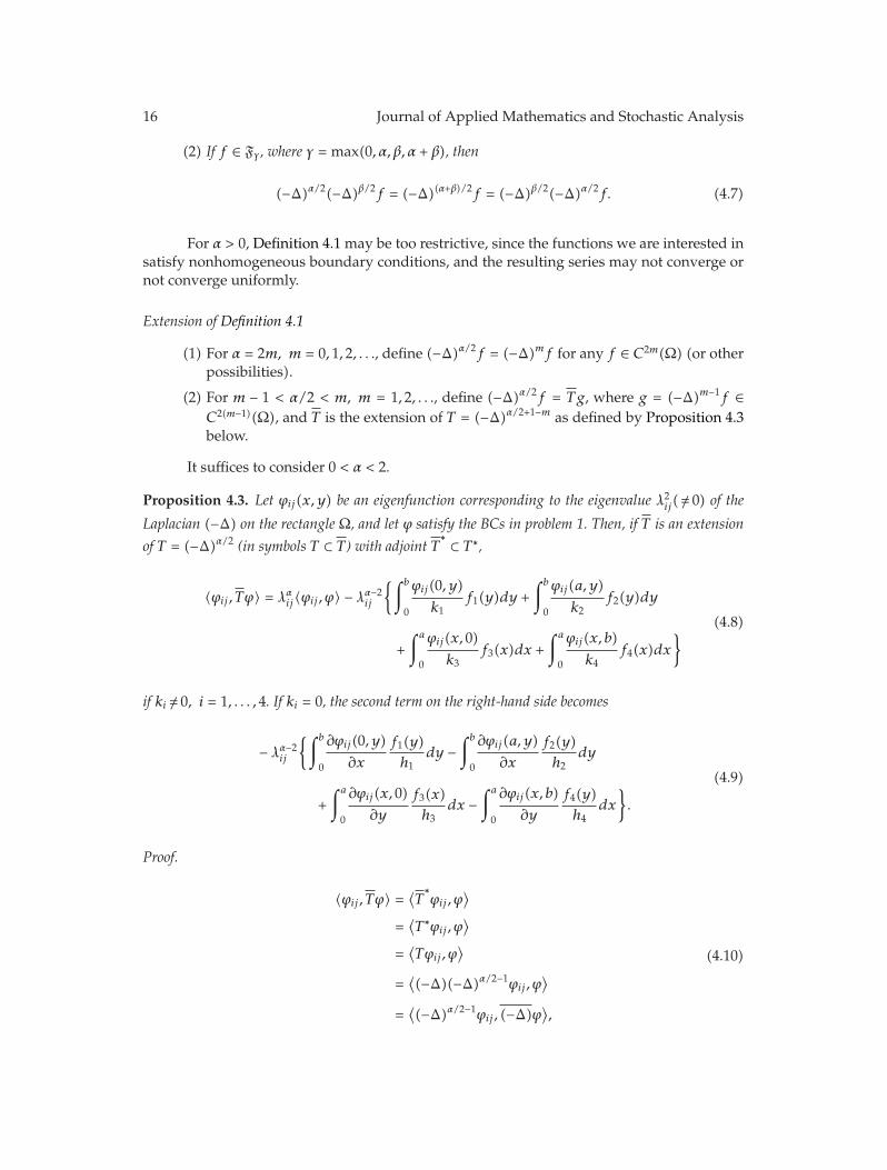
Proposition 4.3. Let ϕij(x, y) be an eigenfunction corresponding to the eigenvalue λ2ij(/= 0) of the
Laplacian (−Δ) on the rectangle Ω, and let ϕ satisfy the BCs in problem 1. Then, if T is an extension
of T = (−Δ)α/2 (in symbols T ⊂ T ) with adjoint T∗⊂ T ∗,
〈ϕij , Tϕ〉 = λαij〈ϕij , ϕ〉 − λα−2ij
{∫b
0
ϕij(0, y)k1
f1(y)dy +∫b
0
ϕij(a, y)k2
f2(y)dy
+∫a
0
ϕij(x, 0)k3
f3(x)dx +∫a
0
ϕij(x, b)k4
f4(x)dx}
(4.8)
if ki /= 0, i = 1, . . . , 4. If ki = 0, the second term on the right-hand side becomes
− λα−2ij
{∫b
0
∂ϕij(0, y)∂x
f1(y)h1
dy −∫b
0
∂ϕij(a, y)∂x
f2(y)h2
dy
+∫a
0
∂ϕij(x, 0)∂y
f3(x)h3
dx −∫a
0
∂ϕij(x, b)∂y
f4(y)h4
dx
}
.
(4.9)
Proof.
〈ϕij , Tϕ〉 =⟨
T∗ϕij , ϕ
⟩
=⟨
T ∗ϕij , ϕ⟩
=⟨
Tϕij , ϕ⟩
=⟨
(−Δ)(−Δ)α/2−1ϕij , ϕ⟩
=⟨
(−Δ)α/2−1ϕij , (−Δ)ϕ⟩
,
(4.10)

M. Ilic et al. 17
where (−Δ) is the extension of (−Δ) with domain D′(Ω) that is the same as D(Ω) withoutB(ϕ) = 0, which is well documented in books on partial differential equations [7]. This isdone by calculating the conjunct (concomitant or boundary form) using the Green’s formula
∫∫
Ω(v∇2u − u∇2v)dS =
∫
∂Ω
(
v∂u
∂n− u∂v
∂n
)
ds. (4.11)
Thus,
⟨
ϕij , Tϕ〉 = λα−2ij
⟨
ϕij , (−Δ)ϕ〉
= −λα−2ij
∫∫
Ωϕij∇2ϕdS
= −λα−2ij
{∫∫
Ωϕ∇2ϕij dS +
∫
∂Ω
(
ϕij∂ϕ
∂n− ϕ
∂ϕij
∂n
)
ds
}
(4.12)
which gives the result on substitution.
This result can be readily used to write down the analytic solution to the FPE problem.First, we obtain the spectral representation of the operator T by solving the eigenvalueproblem:
−Δϕ = λ2ϕ, B(ϕ) = 0. (4.13)
Knowing the eigenvalues λij and the corresponding orthonormal (ON) eigenfunctions ϕij ,we can use the finite-transform method with respect to ϕij and Proposition 4.3 to obtain
λαij〈ϕij , ϕ〉 = 〈g, ϕij〉 + λα−2ij bij , (4.14)
where λα−2ij bij is the second term on the right hand side in Proposition 4.3. Hence,
ϕ(x, y) =∞∑
i=1
∞∑
j=1
〈g, ϕij〉λαij
ϕij(x, y) +∞∑
i=1
∞∑
j=1
bij
λ2ij
ϕij(x, y). (4.15)
5. Results and discussion
In this section, we exhibit the results of applying Algorithm 2.4 to solve two FPE testproblems. To assess the accuracy of our approximation, we compare the numerical solutionswith the exact solution in each case.

18 Journal of Applied Mathematics and Stochastic Analysis
Test problem 1: FPE with Dirichlet boundary conditions
Solve (−∇2)α/2ϕ = g0/k on the unit square [0, 1] × [0, 1] subject to the type I boundary
conditions ϕ = 0 on boundary ∂Ω. For this problem, the ON eigenfunctions are given by
ϕij = {2 sin(iπx) sin(jπy)}∞i,j=1, (5.1)
and the corresponding eigenvalues λ2ij = π
2(i2+j2). The analytical solution is then given fromSection 4 as
ϕ(x, y) =16g0
kπ2
∞∑
i=0
∞∑
j=0
sin[(2i + 1)πx] sin[(2j + 1)πy]
(2i + 1)(2j + 1)[(2i + 1)2π2 + (2j + 1)2π2]α/2. (5.2)
For the numerical solution, a standard five-point finite-difference formula with equal gridspacing h = 1/n in the x and y directions has been used to generate the block tridiagonalmatrix A ∈ R
(n−1)2×(n−1)2given in (2.1) as
A =
⎡
⎢
⎢
⎢
⎢
⎢
⎢
⎣
B −I−I B −I
. . . . . . . . .−I B −I−I B
⎤
⎥
⎥
⎥
⎥
⎥
⎥
⎦
where B =
⎡
⎢
⎢
⎢
⎢
⎢
⎢
⎣
4 −1−1 4 −1−1 4 −1
. . . . . . −1−1 4
⎤
⎥
⎥
⎥
⎥
⎥
⎥
⎦
∈ R(n−1)×(n−1). (5.3)
The parameters used to test this model are listed in Table 1.
Test problem 2: FPE with mixed boundary conditions
Solve (−∇2)α/2ϕ = g0/k on the unit square [0, 1]×[0, 1] subject to type III boundary conditions
−∂ϕ
∂x+H1ϕ = H1ϕ∞ at x = 0,
∂ϕ
∂x+H2ϕ = H2ϕ∞ at x = 1,
−∂ϕ
∂y+H3ϕ = H3ϕ∞ at y = 0,
∂ϕ
∂y+H4ϕ = H4ϕ∞ at y = 1,
(5.4)
where Hi = hi/k. The analytical solution to this problem is given by
ϕ(x, y) = ϕ∞ +g0
k
∞∑
i=1
∞∑
j=1
αi,jX(μi, x)Y (νj , y)
(μ2i + ν
2j )α/2Nx(μi)Ny(νj)
, (5.5)
M. Ilic et al. 19
Table 1: Physical parameters for test problem 1.
Parameter Description Valuek Thermal conductivity 1 Wm−1 K−1
g0 Source 10 Wm−3
α Fractional index 0.5,1,1.5
where the eigenfunctions are
X(μi, x) = μi cos(μix) +H1 sin(μix), Y (νj , y) = νj cos(νjy) +H3 sin(νjy), (5.6)
with normalisation factors
N2x(μi) =
12
[
(
μ2i +H
21
)
(
1 +H2
μ2i +H
22
)
+H1
]
,
N2y(νj) =
12
[
(
ν2j +H
23)
(
1 +H4
ν2j +H
24
)
+H3
]
.
(5.7)
The eigenvalues μi are determined by finding the roots of the transcendental equation:
tan(μ) =μ(H1 +H2)μ2 −H1H2
(5.8)
with νj determined from a similar equation for ν. Finally, αi,j is given by
αi,j =∫∫1
0
X(μi, ξ)Y (νj , η)Nx(μi)Ny(νj)
dξ dη . (5.9)
For the numerical solution, a standard five-point finite-difference formula with equalgrid spacing h = 1/nwas again employed in the x and y directions. However in this example,additional finite-difference equations are required for the boundary nodes as a result of typeIII boundary conditions. The block tridiagonal matrix required in (2.8) is then similar to thatexhibited for example 1, however it has dimension A ∈ R
(n+1)2×(n+1)2and boundary blocks
must be modified to account for the boundary condition contributions.The parameter values used for this problem are listed in Table 2.
5.1. Discussion of results for test problem 1
A comparison of the numerical and analytical solutions for test problem 1 is exhibited inFigure 1 for different values of the fractional index α = 0.5, 1.0, 1.5, and 2 (with the value 2representing the solution of the classical Poisson equation). In all cases, it can be observedthat good agreement is obtained between theory and simulation, with the analytical (solidcontour lines) and numerical (dashed contour lines) solutions almost indistinguishable. Infact, Algorithm 2.4 consistently produced a numerical solution within approximately 2%absolute error of the analytical solution.

20 Journal of Applied Mathematics and Stochastic Analysis
Table 2: Physical parameters for test problem 2.
Parameter Description Valuek Thermal conductivity 5 Wm−1 K−1
g0 Source −10 Wm−3
h1, h3 Heat transfer coefficient 0 Wm−2 K−1
h2, h4 Heat transfer coefficient 2 Wm−2 K−1
ϕ∞ External temperature 20 Kα Fractional index 0.5,1,1.5
00.10.20.30.40.50.60.70.80.9
1
0 0.2 0.4 0.6 0.8 1
0.511.522.533.544.55
(a)
00.10.20.30.40.50.60.70.80.9
1
0 0.2 0.4 0.6 0.8 1
0.5
1
1.5
2
2.5
(b)
00.10.20.30.40.50.60.70.80.9
1
0 0.2 0.4 0.6 0.8 1
0.2
0.4
0.6
0.8
1
1.2
1.4
(c)
00.10.20.30.40.50.60.70.80.9
1
0 0.2 0.4 0.6 0.8 1
0.1
0.2
0.3
0.4
0.5
0.6
0.7
(d)
Figure 1: Comparisons of numerical (dashed lines) and analytical solutions (solid lines) for test problem1 computed using Algorithm 2.4: (a) α = 0.5, (b) α = 1.0, (c) α = 1.5, and (d) α = 2 (classical case).
The impact of decreasing the fractional index from α = 2 to 0.5 is particularly evidentin Figure 2 from the shape and magnitude of the computed three-dimensional symmetricprofiles. Low values of α produce a solution exhibiting a pronounced hump-like shape, withthe diffusion rate low, the magnitude of the solution high at the centre, and steep gradientsevident near the boundary of the solution domain. As α increases, the magnitude of theprofile diminishes and the solution is much more diffuse and representative of a Gaussianprocess. These observations motivate the following remark.
Remark 5.1. Over Rn, the Riesz operator (−Δ)α/2 as defined by
(−Δ)α/2f(x) =1
g(α)
∫
Rn
|x − y|α−nf(y)dy, (5.10)

M. Ilic et al. 21
01
2
3
4
5
1
0.5
0 0 0.2 0.4 0.6 0.81
(a)
01
2
3
4
5
1
0.5
0 0 0.2 0.4 0.6 0.81
(b)
01
2
3
4
5
1
0.5
0 0 0.2 0.4 0.6 0.81
(c)
01
2
3
4
5
1
0.5
0 0 0.2 0.4 0.6 0.81
(d)
Figure 2: Numerical solutions for test problem 1: (a) α = 0.5, (b) α = 1.0, (c) α = 1.5, and (d) α = 2 (classicalcase).
where f is a C∞- function with rapid decay at infinity, and
g(α) =πn/22αΓ(α/2)Γ(n/2 − α/2)
(5.11)
is known to generate α-stable processes. In fact, the Green’s function of the equation
∂p
∂t= −(−Δ)α/2p(t, x), T > 0, x ∈ R (5.12)
is the probability density function of a symmetric α-stable process. When α = 1, it is thedensity function of a Cauchy distribution, and when α = 2 it is the classical Gaussian density.As α → 0, the tail of the density function is heavier and heavier. These behaviours arereflected in the numerical results given in the above example; namely, when α → 2, theplots exhibit the bell shape of the Gaussian density, but when α → 0, the curves are flatter,indicating very heavy tails as expected.
We now report on the performance of Algorithm 2.4 for computing the solution of theFPE. The numerical solutions shown in Figures 1 and 2 were generated using a standard five-point finite difference stencil to construct the matrix representation of the two-dimensionalLaplacian operator. The x- and y-dimensions were divided equally into 31 divisions to

22 Journal of Applied Mathematics and Stochastic Analysis
−20
−15
−10
−5
0
5
log 10‖e
rror‖ 2
0 25 50 75 100 125 150
Matrix vector multiplies
‖r‖ stage 1Optimal
A−qv
Bound
Stage 1 Stage 2
No subspace
recycling
Figure 3: Residual reduction for test problem 1 computed using the two-stage process outlined inAlgorithm 2.4.
produce the symmetric positive definite matrix A ∈ R900×900 having its spectrum σ(A) ⊂
[0.0205, 7.9795]. One notes for this problem that the homogeneous boundary conditionsnecessitate only the solution Φ = hαA−α/2g. Algorithm 2.4 was still employed in this case;however in stage 1 we at first solve Ax = g by the adaptively preconditioned thick restartprocedure. The gathered spectral information from stage 1 is then used for the efficientcomputation of Φ during stage 2.
Figure 3 depicts the reduction in the residual of the linear system and the errorin the matrix function approximation during both stages of the solution process for testproblem 1 for the case α = 1. For this test using FOM(25,10), (subspace size 25 with anadditional 10 approximate Ritz vectors augmented at the front of the Krylov subspace) fourrestarts were required to reduce the linear system residual to ≈ 1 × 10⁻¹⁵, which representedan overall total of 110 matrix-vector products. This low tolerance was enforced to ensurethat as many approximate eigenpairs of A could be computed and then locked duringstage 1 for use in stage 2. An eigenpair was deemed converged when the residual in theapproximate eigenpair was less than θmax × 10−10, where θmax is the current estimate of thelargest eigenvalue of A. This process saw 1 eigenpair locked after 2 restarts, 5 locked after 3restarts, and finally 9 locked after 4 restarts. From this figure, we also see that when subspacerecycling is used for stage 2 only an additional 30 matrix-vector products are required tocompute the solution Φ to an acceptable accuracy. It is also worth pointing out that theLanczos approximation for this preconditioned matrix function reduces much more rapidlythan for the case where preconditioning (dotted line) is not used. Furthermore, the Lanczosapproximation in this example lies almost entirely on the curve that represents the optimalapproximation obtainable from the Krylov subspace [26]. Finally, we see that the bound (3.9)can be used with confidence as a means for halting stage 2 once the desired accuracy in thebound is reached.
5.2. Discussion of results for test problem 2
A comparison of the numerical and analytical solutions for test problem 2 is exhibited inFigure 4, again for the values of the fractional index α = 0.5, 1.0, 1.5, and 2. It can be seenthat the agreement between theory and simulation is more than acceptable for this case, withAlgorithm 2.4 producing a numerical solution within approximately 4% absolute error of the

M. Ilic et al. 23
00.10.20.30.40.50.60.70.80.9
1
0 0.1 0.2 0.3 0.4 0.5 0.6 0.7 0.8 0.9 1
17.75
17.8
17.85
17.9
17.95
18
18.05
18.1
(a)
00.10.20.30.40.50.60.70.80.9
1
0 0.1 0.2 0.3 0.4 0.5 0.6 0.7 0.8 0.9 1
17.5
17.6
17.7
17.8
17.9
18
(b)
00.10.20.30.40.50.60.70.80.9
1
0 0.1 0.2 0.3 0.4 0.5 0.6 0.7 0.8 0.9 1
17.2
17.3
17.4
17.5
17.6
17.7
17.8
17.9
(c)
00.10.20.30.40.50.60.70.80.9
1
0 0.1 0.2 0.3 0.4 0.5 0.6 0.7 0.8 0.9 116.9
17
17.1
17.2
17.3
17.4
17.5
17.6
17.7
(d)
Figure 4: Comparisons of numerical (dashed line) and analytical solutions (solid line) for test problem 2computed using Algorithm 2.4: (a) α = 0.5, (b) α = 1.0, (c) α = 1.5, and (d) α = 2 (classical case).
analytical solution. However, the impact of increasing the fractional index from α = 0.5 to 2is less dramatic for problem 2.
The numerical solutions shown in Figure 4 were again generated using a standard five-point finite-difference stencil to construct the matrix representation of the two-dimensionalLaplacian operator. The x- and y-dimensions were divided equally into 30 divisionsresulting in the symmetric positive definite matrix A ∈ R
961×961 having its spectrumσ(A) ⊂ [0.000758, 7.9795]. One notes for this problem that type II boundary conditions haveproduced a small eigenvalue that undoubtedly will hinder the performance of restarted FOM.
Figure 5 depicts the reduction in the residual of the linear system for computing thesolution Φ1 and the error in the matrix function approximation for Φ2 during both stagesof the solution process for test problem 2 with α = 1. Using FOM(25,10), a total of ninerestarts were required to reduce the linear system residual to ≈ 1×10⁻¹⁵, which represented anoverall total of 240 matrix-vector products. One notes that this is much higher than Problem1 and primarily due to the occurrence of small eigenvalues in σ(A). The thick restart processsaw 1 eigenpair locked after 5 restarts, 4 locked after 6 restarts, and finally 10 locked after9 restarts. From this figure, we also see that when subspace recycling is used for stage 2only an additional 25 matrix-vector products are required to compute the solution Φ2 toan acceptable accuracy, which is clearly much less than the unpreconditioned (dotted line)case. The Lanczos approximation in this example again lies almost entirely on the curve thatrepresents the optimal approximation obtainable from the Krylov subspace. Finally, we seethat the bound (3.9) can be used to halt stage 2 once the desired accuracy is reached.

24 Journal of Applied Mathematics and Stochastic Analysis
−16−14−12−10−8−6−4−2
024
log 10‖e
rror‖ 2
0 50 100 150 200 250 300
Matrix vector multiplies
‖r‖ stage 1Optimal
A−qv
Bound
Stage 1 Stage 2
No subspace
recycling
Figure 5: Residual reduction for test problem 2 computed using the two-stage process outlined inAlgorithm 2.4.
6. Conclusions
In this work, we have shown how the fractional Poisson equation can be approximatelysolved using a finite-difference discretisation of the Laplacian to produce an appropriatematrix representation of the operator. We then derived a matrix equation that involved botha linear system solution and a matrix function approximation with the matrix A raised to thesame fractional index as the Laplacian. We proposed an algorithm based on Krylov subspacemethods that could be used to efficiently compute the solution of this matrix equation using atwo-stage process. During stage 1, we used an adaptively preconditioned thick restarted FOMmethod to approximately solve the linear system and then used recycled spectral informationgathered during this restart process to accelerate the convergence of the matrix functionapproximation in stage 2. Two test problems were then presented to assess the accuracy of ouralgorithm, and good agreement with the analytical solution was noted in both cases. Futureresearch will see higher dimensional fractional diffusion equations solved using a similarapproach via the finite volume method.
Acknowledgment
This work was supported financially by the Australian Research Council Grant no.LP0348653.
References
[1] F. Lorenzo and T.T. Hartley, “Initialization, conceptualization, and application in the generalizedfractional calculus,” Tech. Rep. NASA/TP—208415, NASA Center for Aerospace Information,Hanover, Md, USA, 1998.
[2] R. Metzler and J. Klafter, “The random walk’s guide to anomalous diffusion: a fractional dynamicsapproach,” Physics Reports, vol. 339, no. 1, pp. 1–77, 2000.
[3] R. Metzler and J. Klafter, “The restaurant at the end of the random walk: recent developments in thedescription of anomalous transport by fractional dynamics,” Journal of Physics A, vol. 37, no. 31, pp.R161–R208, 2004.
[4] D. A. Benson, S. W. Wheatcraft, and M. M. Meerschaert, “Application of a fractional advectiondisper-sion equation,” Water Resources Research, vol. 36, no. 6, pp. 1403–1412, 2000.
[5] D. A. Benson, S. W. Wheatcraft, and M. M. Meerschaert, “The fractional-order governing equation oflevy motion,” Water Resources Research, vol. 36, no. 6, pp. 1413–1423, 2000.

M. Ilic et al. 25
[6] M. M. Meerschaert, J. Mortensen, and S. W. Wheatcraft, “Fractional vector calculus for fractionaladvection-dispersion,” Physica A, vol. 367, pp. 181–190, 2006.
[7] B. Friedman, Principles and Techniques of Applied Mathematics, John Wiley & Sons, New York, NY, USA,1966.
[8] M. Ilic, F. Liu, I. W. Turner, and V. Anh, “Numerical approximation of a fractional-in-space diffusionequation—II-with nonhomogeneous boundary conditions,” Fractional Calculus & Applied Analysis,vol. 9, no. 4, pp. 333–349, 2006.
[9] B. J. West and V. Seshadri, “Linear systems with Levy fluctuations,” Physica A, vol. 113, no. 1-2, pp.203–216, 1982.
[10] R. Gorenflo and F. Mainardi, “Random walk models for space-fractional diffusion processes,”Fractional Calculus & Applied Analysis, vol. 1, no. 2, pp. 167–191, 1998.
[11] R. Gorenflo and F. Mainardi, “Approximation of Levy-Feller diffusion by random walk,” Journal forAnalysis and Its Applications, vol. 18, no. 2, pp. 231–246, 1999.
[12] I. P. Gavrilyuk, W. Hackbusch, and B. N. Khoromskij, “Data-sparse approximation to the operator-valued functions of elliptic operator,” Mathematics of Computation, vol. 73, no. 247, pp. 1297–1324,2004.
[13] W. Hackbusch and B. N. Khoromskij, “Low-rank Kronecker-product approximation to multidimen-sional nonlocal operators—part I. Separable approximation of multi-variate functions,” Computing,vol. 76, no. 3, pp. 177–202, 2006.
[14] W. Hackbusch and B. N. Khoromskij, “Low-rank Kronecker-product approximation to multidimen-sional nonlocal operators—part II. HKT representation of certain operators,” Computing, vol. 76, no.3, pp. 203–225, 2006.
[15] M. Ilic, F. Liu, I. W. Turner, and V. Anh, “Numerical approximation of a fractional-in-space diffusionequation—I,” Fractional Calculus & Applied Analysis, vol. 8, no. 3, pp. 323–341, 2005.
[16] G. Gripenberg and I. Norros, “On the prediction of fractional Brownian motion,” Journal of AppliedProbability, vol. 33, no. 2, pp. 400–410, 1996.
[17] Y. Hu, “Prediction and translation of fractional Brownian motions,” in Stochastics in Finite and InfiniteDimensions, T. Hida, R. L. Karandikar, H. Kunita, B. S. Rajput, S. Watanabe, and J. Xiong, Eds., Trendsin Mathematics, pp. 153–171, Birkhauser, Boston, Mass, USA, 2001.
[18] G. H. Golub and C. F. Van Loan, Matrix Computations, Johns Hopkins Studies in the MathematicalSciences, The Johns Hopkins University Press, Baltimore, Md, USA, 3rd edition, 1996.
[19] Y. Saad, Iterative Methods for Sparse Linear Systems, SIAM, Philadelphia, Pa, USA, 2nd edition, 2003.[20] H. A. van der Vorst, Iterative Krylov Methods for Large Linear Systems, vol. 13 of Cambridge Monographs
on Applied and Computational Mathematics, Cambridge University Press, Cambridge, UK, 2003.[21] N. J. Higham, Functions of Matrices: Theory and Computation, SIAM, Philadelphia, Pa, USA, 2008.[22] V. Druskin and L. Knizhnerman, “Krylov subspace approximation of eigenpairs and matrix functions
in exact and computer arithmetic,” Numerical Linear Algebra with Applications, vol. 2, no. 3, pp. 205–217,1995.
[23] M. Hochbruck and C. Lubich, “On Krylov subspace approximations to the matrix exponentialoperator,” SIAM Journal on Numerical Analysis, vol. 34, no. 5, pp. 1911–1925, 1997.
[24] M. Eiermann and O. G. Ernst, “A restarted Krylov subspace method for the evaluation of matrixfunctions,” SIAM Journal on Numerical Analysis, vol. 44, no. 6, pp. 2481–2504, 2006.
[25] L. Lopez and V. Simoncini, “Analysis of projection methods for rational function approximation tothe matrix exponential,” SIAM Journal on Numerical Analysis, vol. 44, no. 2, pp. 613–635, 2006.
[26] J. van den Eshof, A. Frommer, T. Lippert, K. Schilling, and H. A. van der Vorst, “Numerical methodsfor the QCD overlap operator—I. Sign-function and error bounds,” Computer Physics Communications,vol. 146, pp. 203–224, 2002.
[27] M. Ilic and I. W. Turner, “Approximating functions of a large sparse positive definite matrix using aspectral splitting method,” The ANZIAM Journal, vol. 46(E), pp. C472–C487, 2005.
[28] M. Ilic, I. W. Turner, and A. N. Pettitt, “Bayesian computations and efficient algorithms for computingfunctions of large, sparse matrices,” The ANZIAM Journal, vol. 45(E), pp. C504–C518, 2004.
[29] R. B. Lehoucq and D. C. Sorensen, “Deflation techniques for an implicitly restarted Arnoldi iteration,”SIAM Journal on Matrix Analysis and Applications, vol. 17, no. 4, pp. 789–821, 1996.
[30] A. Stathopoulos, Y. Saad, and K. Wu, “Dynamic thick restarting of the Davidson, and the implicitlyrestarted Arnoldi methods,” SIAM Journal on Scientific Computing, vol. 19, no. 1, pp. 227–245, 1998.
[31] M. Ilic and I. W. Turner, “Krylov subspaces and the analytic grade,” Numerical Linear Algebra withApplications, vol. 12, no. 1, pp. 55–76, 2005.

26 Journal of Applied Mathematics and Stochastic Analysis
[32] R. B. Morgan, “A restarted GMRES method augmented with eigenvectors,” SIAM Journal on MatrixAnalysis and Applications, vol. 16, no. 4, pp. 1154–1171, 1995.
[33] J. Baglama, D. Calvetti, G. H. Golub, and L. Reichel, “Adaptively preconditioned GMRES algorithms,”SIAM Journal on Scientific Computing, vol. 20, no. 1, pp. 243–269, 1998.
[34] J. Erhel, K. Burrage, and B. Pohl, “Restarted GMRES preconditioned by deflation,” Journal ofComputational and Applied Mathematics, vol. 69, no. 2, pp. 303–318, 1996.
[35] R. V. Churchill, Complex Variables and Applications, McGraw-Hill, New York, NY, USA, 2nd edition,1960.