Embed Size (px)
Citation preview

A Numerical Optimization Approach
to General Graph Drawing
Daniel Tunkelang
January 1999
CMU-CS-98-189
School of Computer Science
Carnegie Mellon University
Pittsburgh, PA 15213
Submitted in partial fulfillment of the requirements
for the degree of Doctor of Philosophy
Thesis Committee:
Daniel Sleator, Chair
Paul Heckbert
Bruce Maggs
Omar Ghattas, Civil and Environmental Engineering
Mark Wegman, IBM T . J. Watson Research Center
Copyright © 1999 Daniel Tunkelang
This research was supported by the National Science Foundation under grant number DMS-9509581. The views and conclusions contained in this document are those of the author and shouldnot be interpreted as representing the official policies, either expressed or implied, of the NAF or theU.S. government.

Keywords: visualization, graph drawing, numerical optimization, force-directed
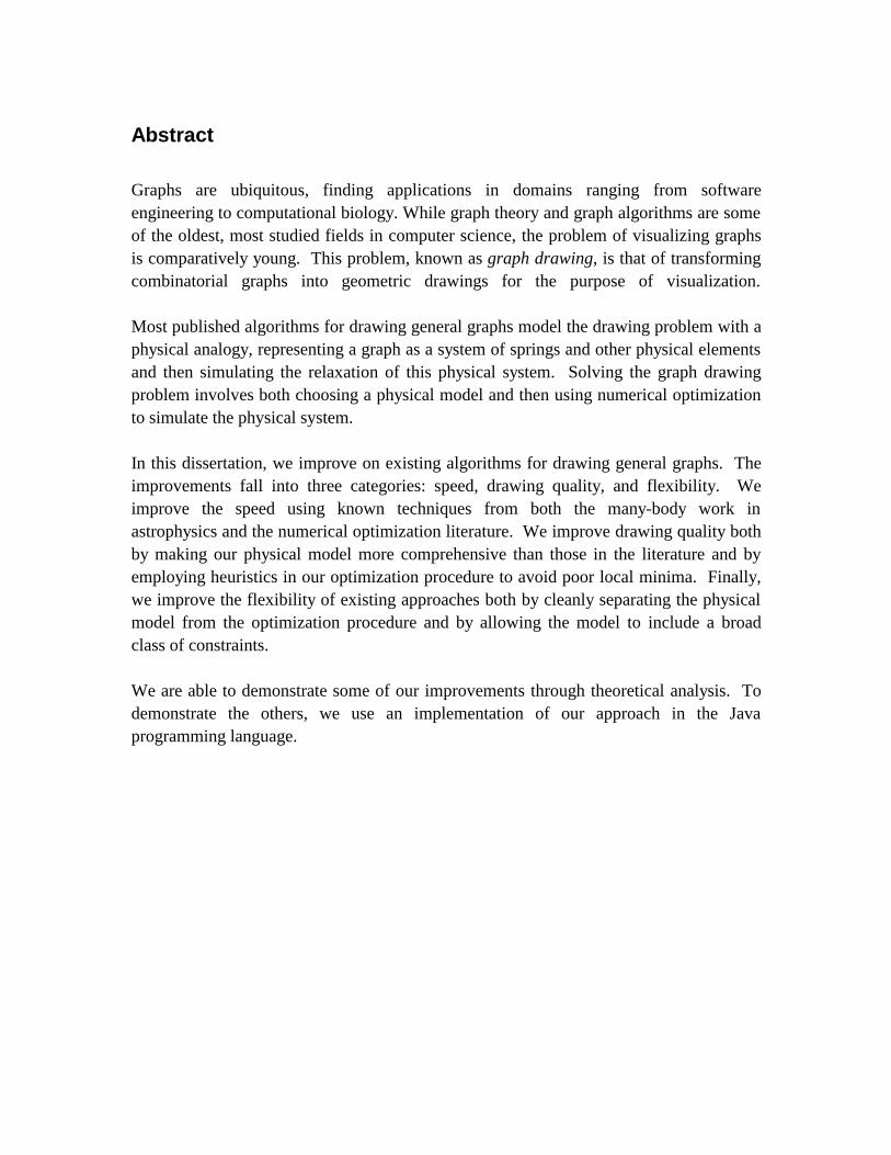
Abstract
Graphs are ubiquitous, finding applications in domains ranging from softwareengineering to computational biology. While graph theory and graph algorithms are someof the oldest, most studied fields in computer science, the problem of visualizing graphsis comparatively young. This problem, known as graph drawing, is that of transformingcombinatorial graphs into geometric drawings for the purpose of visualization.
Most published algorithms for drawing general graphs model the drawing problem with aphysical analogy, representing a graph as a system of springs and other physical elementsand then simulating the relaxation of this physical system. Solving the graph drawingproblem involves both choosing a physical model and then using numerical optimizationto simulate the physical system.
In this dissertation, we improve on existing algorithms for drawing general graphs. Theimprovements fall into three categories: speed, drawing quality, and flexibility. Weimprove the speed using known techniques from both the many-body work inastrophysics and the numerical optimization literature. We improve drawing quality bothby making our physical model more comprehensive than those in the literature and byemploying heuristics in our optimization procedure to avoid poor local minima. Finally,we improve the flexibility of existing approaches both by cleanly separating the physicalmodel from the optimization procedure and by allowing the model to include a broadclass of constraints.
We are able to demonstrate some of our improvements through theoretical analysis. Todemonstrate the others, we use an implementation of our approach in the Javaprogramming language.

Acknowledgments
First, I would like to thank my advisor, Danny Sleator, and the other members of my
committee: Paul Heckbert, Omar Ghattas, Bruce Maggs, and Mark Wegman. I am
especially grateful that they allowed me to pursue a dissertation in an area somewhat
removed from their primary fields of research, advising me according to their respective
strengths. Their feedback was essential to the quality of this dissertation.
I am greatly indebted to Carnegie Mellon University for providing both the funding and
the intellectual environment that were essential to my work. I especially thank my former
housemate, Jonathan Shewchuk, and my officemates, Girija Narlikar and Chris Okasaki,
for engaging me in discussions across the gamut of computer science. A list of all of the
people who formed my experience at CMU would double this size of this dissertation, but
some names are indispensable: Avrim Blum, Andrew Kompanek, Corey Kosak, Sean
Slattery, and Alma Whitten.
I owe my interest in graph drawing to Mark Wegman, who introduced me to the area
when I was an MIT undergraduate co-op student at the IBM T. J. Watson Research
Center. I thank Mark and Charles Leiserson again for supervising my Master’s Thesis,
and I thank others at IBM for numerous discussions and encouragement: Rangachari
Anand, Lisa Brown, Roy Byrd, Jim Cooper, Doug Kimmelman, Alan Marwick, V. T.
Rajan, and Tova Roth.
My family and friends have always been invaluable, but especially during the ordeal of
completing my dissertation. I cannot thank my parents and brother enough for putting up
with my ever-changing moods during this trying time. Likewise, my closest friends,
Marissa Billowitz and Bilal Khan, sustained me through many trying days and nights.
Finally, I would like to thank all of the teachers who nurtured my interests in mathematics
and computer science through two decades of schooling. Above all, I thank Gian-Carlo
Rota, whom I can finally take up on his promise to let me take him out to dinner after
obtaining my Ph.D.

Table of Contents
1. Introduction..................................................................................................................................7
2. What is Graph Drawing? .............................................................................................................9
2.1. Drawing Conventions..........................................................................................................12
2.2. Constraints...........................................................................................................................13
2.3. Preferences ..........................................................................................................................14
2.4. Summary..............................................................................................................................15
3. Previous Work............................................................................................................................16
3.1. Algorithms for Specific Classes of Graphs .........................................................................16
3.1.1. Trees .............................................................................................................................16
3.1.2. Directed Acyclic Graphs...............................................................................................18
3.1.3. Planar Graphs................................................................................................................20
3.2. Algorithms for General Graphs...........................................................................................21
3.2.1. The Topology-Shapes-Metrics Approach.....................................................................21
3.2.2. The Force-Directed Approach ......................................................................................22
4. The Force-Directed Approach ...................................................................................................23
4.1. The Spring Embedder Model ..............................................................................................23
4.2. Kamada and Kawai’s Approach..........................................................................................24
4.3. Fruchterman and Reingold’s Approach ..............................................................................25
4.4. Models that Address Edge Crossings..................................................................................26
4.5. Computational Complexity .................................................................................................26
4.6. Other Force-Directed Work.................................................................................................27
4.7. Summary of Problems in Published Approaches ................................................................27
5. Modeling Graph Drawing as an Optimization Problem ............................................................29
5.1. Output Variables .................................................................................................................29
5.2. Force Laws ..........................................................................................................................29
5.2.1. Springs ..........................................................................................................................30
5.2.2. Vertex-Vertex Repulsion..............................................................................................32
5.2.3. Vertex-Edge Repulsion.................................................................................................34
5.3. Constraints...........................................................................................................................35
5.3.1. Penalty Functions..........................................................................................................35
5.3.2. Constraints versus Preferences .....................................................................................35
6. Computing the Gradient Efficiently...........................................................................................37
6.1. Computing the Gradient Naïvely.........................................................................................37
6.2. Simple θ(n) Approximations for Computing Vertex-Vertex Repulsion.............................38
6.2.1. Distance Cut-Offs .........................................................................................................38
6.2.2. Centripetal Repulsion ...................................................................................................40

6.3. Approximating Vertex-Vertex Repulsion Forces in θ(n log n) Time .................................42
6.3.1. Building the Quad-Tree ................................................................................................43
6.3.2. Computing the Force on Each Particle .........................................................................45
6.3.3. Applying Barnes-Hut to Compute Vertex-Vertex Repulsion Forces ...........................47
6.4. Computing Vertex-Edge Repulsion Forces.........................................................................47
7. The Optimization Procedure ......................................................................................................49
7.1. The Method of Steepest Descent.........................................................................................49
7.2. The Newton Direction.........................................................................................................51
7.3. The Conjugate Gradient Method.........................................................................................52
7.4. The Conjugate Gradient Method with Restarts...................................................................53
7.5. Computing the Step Size .....................................................................................................54
8. Making the Gradient Time-Dependent ......................................................................................56
8.1. Making the Gradient Smoother in the Early Iterations .......................................................56
8.1.1. Capping Spikes .............................................................................................................57
8.1.2. Strengthening the Long-Range Vertex-Vertex Repulsion Forces ................................58
8.2. Using Exterior Penalties to Incorporate Constraints...........................................................58
8.3. Introducing Additional Degrees of Freedom.......................................................................60
9. Vertex Size and Shape ...............................................................................................................62
9.1. Vertex Radii ........................................................................................................................62
9.2. Adapting the Force Laws to Consider Vertex Radii ...........................................................63
9.2.1. Increasing the Rest Length of Edge Springs.................................................................63
9.2.2. Modifying the Vertex-Vertex Repulsion Law..............................................................64
9.2.3. Modifying the Vertex-Vertex Repulsion Law..............................................................64
9.3. Adapting the Procedure to Compute the Forces..................................................................65
10. Qualitative Results: A Gallery of Examples............................................................................66
10.1. Trees ..................................................................................................................................66
10.2. Planar Biconnected Graphs ...............................................................................................69
10.3. Sparse Non-Planar Graphs ................................................................................................72
10.4. Dense Graphs ....................................................................................................................74
11. Quantitative Results .................................................................................................................77
11.1. Computational Complexity ...............................................................................................77
11.2. Number of Iterations .........................................................................................................78
11.3. Running Time....................................................................................................................82
12. Conclusions and Future Work .................................................................................................84
Bibliography...................................................................................................................................87
1. Introduction
In 1979, Wetherell and Shannon concluded a paper on “Tidy Drawing of Trees” by
saying, “We are currently studying methods for the tidy display of other graph structures,
a subject not covered in the literature” [WS79]. In the past two decades, graph drawing
has become a vibrant research area. An annotated bibliography from 1994 [DETT94]
lists over 300 relevant publications, and these do not include the dozens of papers and
systems presented at the annual symposia on graph drawing since 1993. More recently,
the authors of the bibliography have published a textbook [DETT99] on graph drawing.
Most of the work, however, considers special cases. A quarter of the papers in the
annotated bibliography address the problem of computing planar (crossing-free) drawings
of planar graphs. A comparable fraction of the work considers layered drawings of
directed acyclic graphs. While this specificity attests to the relative importance of certain
classes of graphs, it also reflects the difficulty of solving the general problem.
Our work addresses general graph drawing. Although the treatment of special cases can
lead to elegant mathematical results, the practical side of graph drawing requires a greater
emphasis on generality. Our approach, based on numerical optimization, builds on
existing approaches for drawing general graphs. We demonstrate the value of our work
in three ways. First, we show both a theoretical and an empirical improvement in
performance over the published general graph drawing algorithms. Second, we achieve
better drawings by incorporating aesthetic elements that the published approaches do not
take into account. Third, we obtain a more flexible approach by using a numerical
optimization approach that cleanly separates the objective function from the optimization
procedure and allows us to incorporate a general class of constraints into our model.
We begin with an overview of the graph drawing problem and its wide range of
applications. We then review the previous work in the field, focusing on algorithms that
address general graphs. We present a general framework for modeling graph drawing as
a numerical optimization problem, and we show how previous approaches fit into this
framework. We then present our techniques to address performance, drawing quality, and
flexibility. Our principle solutions for the performance problem are to use the Barnes-
Hut procedure to reduce a θ(n2) time computation in the inner loop to θ(n log n) , and
then to replace the commonly used method of steepest descent with the conjugate
gradient method as a more efficient optimization procedure. Our main improvements in
drawing quality come from incorporating vertex-edge distance and vertex shape into our
physical model. Finally, we describe how we incorporate a general class of constraints
into our model by making the objective function time-dependent and using the method of
exterior penalties. In fact, this technique of using a time-dependent objective function not
only makes our approach more flexible, but can also improve both performance and
drawing quality. We present the results of our work both qualitatively, though a gallery
of examples, and quantitatively, through both theoretical and empirical analysis.
2. What is Graph Drawing?
Before we can talk about graph drawing, we must explain what we mean by a graph. A
graph is a collection of entities and their relationships. We refer to the entities as the
vertices of the graph, and to their relationships as edges.1 Each edge pairs two vertices,
which we call its endpoints. When we are discussing a single graph, we will denote it by
G, and we will denote the vertex and edge sets as V and E respectively.
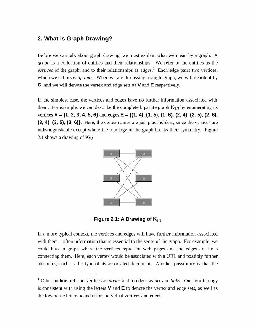
In the simplest case, the vertices and edges have no further information associated with
them. For example, we can describe the complete bipartite graph K3,3 by enumerating its
vertices V = 1, 2, 3, 4, 5, 6 and edges E = (1, 4), (1, 5), (1, 6), (2, 4), (2, 5), (2, 6),
(3, 4), (3, 5), (3, 6). Here, the vertex names are just placeholders, since the vertices are
indistinguishable except where the topology of the graph breaks their symmetry. Figure
2.1 shows a drawing of K3,3.
Figure 2.1: A Drawing of K 3,3
In a more typical context, the vertices and edges will have further information associated
with them—often information that is essential to the sense of the graph. For example, we
could have a graph where the vertices represent web pages and the edges are links
connecting them. Here, each vertex would be associated with a URL and possibly further
attributes, such as the type of its associated document. Another possibility is that the
1 Other authors refer to vertices as nodes and to edges as arcs or links. Our terminology
is consistent with using the letters V and E to denote the vertex and edge sets, as well as
the lowercase letters v and e for individual vertices and edges.

graph could represent a database of terms extracted from a large corpus of text. Here, the
edges could store the nature of the relationships among the terms. Figures 2.2 and 2.3
show examples of graphs that could arise in practical applications.
Figure 2.2: Disciplines and their Common Subfields
Figure 2.3: Six Degrees of Kevin Bacon

One attribute of an edge that we single out is its directedness. An edge can be undirected
or directed, reflecting whether the relationship between the endpoints is symmetric or
asymmetric. We call a graph consisting of only undirected edges an undirected graph
and one consisting of only directed edges a directed graph. If a graph has both undirected
and directed edges, we call it a mixed graph. In this dissertation, we will focus on
undirected graphs. The techniques we describe can be used to draw directed graphs as
well, but other work, which we describe in the following chapter, is more suited to
drawing directed graphs in such a way as to emphasize the directions of edges.
We define graph drawing as the transformation of a graph into a visual representation of
the graph, which we call a drawing. We depict this transformation in Figure 2.4. In a
typical drawing, we map vertices to boxes or circles on a subset of the plane and map
edges to lines connecting the boxes that represent their endpoints.
V = 1, 2, 3, 4, 5, 6, 7, 8
E = (1, 2), (1, 4), (1, 5), (2, 3), (2, 6), (3, 4), (3, 7), (4, 8), (5, 6), (5, 8), (6, 7), (7, 8)
graph drawing algorithm
Figure 2.4: Graph Drawing
Although graph drawing per se is a young field of research, graph drawing as a practical
art predates computer science. Throughout the sciences, people use graphs to represent
systems composed of a large number of interacting components, especially when the
individual components are simple. Physicists and chemists draw graphs that model
interaction among particles. Electrical engineers draw graphs to represent circuits. Social
scientists draw graphs of group interaction. Still, the widest use of graph drawing is in
computer science and information technology, with domains ranging from software
architecture to semantic networks. Often, graphical visualizations of such systems reveal
far more structure than textual ones, as per the cliché that a picture is worth a thousand
words.

Di Battista et al. break down graph drawing requirements into three basic concepts:
drawing conventions, aesthetics, and constraints [DETT99] . We briefly describe each of
these concepts.
2.1. Drawing Conventions
Drawing conventions are the basic rules that define the space of admissible drawings.
Generally, we can think of drawing conventions as global constraints on the space of
drawings. The drawing conventions specify, among other things, the area that can be
used for the drawing. Unless we specify otherwise, we will assume that the drawing area
is a rectangle in the Euclidean plane R2.
Di Battista et al. list some of the more widely used drawing conventions, and Figure 2.5
shows various drawings of the complete graph K4, for which V = 1, 2, 3, 4 and E =
(1, 2), (1, 3), (1, 4), (2, 3), (2, 4), (3, 4) , using some of these conventions:
Polyline Drawing: each edge is represented as a chain of connected line segments; the
chain may bend at the connection points. See Figure 2.5 (a).
Straight-line Drawing: each edge is represented as a single line segment. A special case
of polyline drawing. See Figure 2.5 (b).
Orthogonal Drawing: each edge is represented as chain of alternating horizontal and
vertical line segments. A special case of polyline drawing. See Figure 2.5 (c).
Planar drawing: no two edges cross; requires that the graph be planar. See Figure 2.5 (d).
Upward drawing: all directed edges are represented by lines or curves that strictly
increase in the vertical direction. Requires that the graph have no directed cycles.
See Figure 2.5 (e) below.
Grid Drawing: all vertices, edge crossings, and bend-points have integer coordinates.
Generally, our drawing conventions will include some subset of the above, as well as
other application-dependent considerations. Our main interest will be in straight-line and
upward drawings, since these conventions are the most amenable to numerical
optimization approaches.

1 2 3 4
1 2
3 4
1 2
3 4
2
1 34
1
2
3
4
(a) (b) (c)
(d) (e)
Figure 2.5: Illustration of Various Drawing Conventions for the Graph K 4
We note that none of the above conventions address vertex shape. We will assume that
vertices are represented by circles, ellipses, or rectangles. Often, we will use the space
taken up by a vertex to show a name or some other information (textual or pictorial)
associated with it.
2.2. Constraints
The drawing conventions constrain the general properties of the drawing. Sometimes, we
use explicit constraints to specify the behavior of particular vertices, edges, or subgraphs.
The two primary sources of constraints are semantics and user interaction. Semantics, for
example, might dictate that a given subset of vertices forms a cluster and should be drawn
in a rectangle that does not include any other vertices. A user, after seeing an
automatically produced drawing might decide that the drawing looks better if a particular
vertex is placed to the left of another vertex and then request that the drawing be
recomputed subject to that constraint. Typical constraints concern absolute or relative
vertex placement.

2.3. Preferences
While it is possible for drawing conventions and constraints to fully determine a drawing,
it is often more useful to distinguish between hard constraints and soft preferences. For
example, we could impose a constraint specifying the exact distance between two vertices
in the drawing, or we could incorporate a preference that the distance between the
vertices be close to the desired distance. Preferences have two advantages over
constraints. First, they can be associated with continuous functions, as in the previous
example, while constraint satisfaction is binary. Second, they can always be combined,
even when combining analogous constraints might lead to an inconsistency. For
example, minimizing edge lengths and maximizing the distances between all vertices are
clearly competing goals; they can, however, be combined in the form of weighted
preferences.
Generally speaking, a preference specifies a measure by which we can judge a drawing.
We quantify these preferences by making them weighted terms in an objective function
that measures the overall quality of a drawing. The weights reflect the priority assigned
to each preference.
Di Battista et al. list the following widely used preferences, which they call “aesthetics”:
Crossings: minimization of the number of edge crossings.
Area: minimization of the drawing area. Measured using either the convex hull or the
bounding rectangle. Only meaningful when the drawing conventions prevent the drawing
from being arbitrarily scaled down.
Total Edge Length: minimization of the sums of lengths of edges. Only meaningful when
the drawing conventions prevent the drawing from being arbitrarily scaled down.
Maximum Edge Length: minimization of the maximum lengths of an edge. Only
meaningful when the drawing conventions prevent the drawing from being arbitrarily
scaled down.
Uniform Edge Length: minimization of the variance in edge length. Only meaningful
when the drawing conventions prevent the drawing from being arbitrarily scaled down.

Total Bends: minimization of the total number of edge bends in a polyline drawing.
Maximum Bends: minimization of the maximum number of edge bends per edge in a
polyline drawing.
Uniform Bends: minimization of the variance in the number of edge bends in a polyline
drawing.
Angular Resolution: maximization of the minimum angle between edges incident to the
same vertex in a polyline (especially straight-line) drawing.
Aspect Ratio: minimization of the ratio between the larger and smaller dimensions of the
drawing area.
Symmetry: displaying symmetries of the graph with geometric symmetries.
The sheer variety of criteria enumerated above suggests that aesthetics are more of an art
than a science. Given the subjective nature of aesthetics, there are limits to how
systematic an approach we can take to describing what makes one drawing of a graph
better than another. Nonetheless, these criteria are sufficiently general that we can start
from some subset of them, refining our model to suit the needs of a particular application.
2.4. Summary
By quantifying and combining drawing conventions, constraints, and preferences, we
arrive at formulation of graph drawing as a problem in numerical optimization. The
drawing conventions dictate the variables in our problem space. The constraints define
the feasible portion of the problem space. Finally, the objective function expresses the
weighted combination of preferences and defines the overall measure that we seek to
minimize, subject to the constraints.

3. Previous Work
Although graph drawing as such is a young field, it has already generated a substantial
body of literature. The best general sources of information are the annotated bibliography
[DETT94] , the recently published textbook [DETT99] , and the proceedings of the
annual Symposia on Graph Drawing [GD93, GD94, GD95, GD96, GD97, GD98].
Related fields include computational geometry, combinatorial optimization, visual
languages, and human-computer interfaces. This section describes the small fraction of
that work that is most relevant to the proposed approaches; the reader is encouraged to
consult the above references.
Broadly speaking, there are two kinds of graph drawing algorithms. The first address
specific classes of graphs. Algorithms of the second kind address general graphs and
differ mostly in their choice of optimization strategy.
All of the algorithms that we discuss produce drawings in R2, with vertices represented as
non-overlapping circles (or boxes) and edges as open curves connecting them. They
generally assume that the input graphs are connected, since it is not difficult to compute
the connected components of a graph and draw them separately.
3.1. Algorithms for Specific Classes of Graphs
There are a variety of algorithms designed for specific classes of input graphs. Three
classes that have attracted particular attention are trees, directed acyclic graphs, and
planar graphs.
3.1.1. Trees
Trees, the simplest class of connected graphs, are among the most common structures in
computer science. A tree is a connected, acyclic graph. Most algorithms for drawing
trees assume that all edges are drawn as straight lines directed away from a specified root
vertex. Supowit and Reingold [SR83] outline six widely accepted aesthetic constraints
for what they call a “eumorphous” (well-shaped) drawing of a rooted tree:
1) The height of a vertex (i.e. its vertical distance from the root) should be proportional
to its distance from the root measured in tree branches. Hence, vertices are placed on
discrete horizontal levels.

2) When the children are ordered (e.g. in a binary tree), left children should be placed
strictly to the left of their parents. Similarly, right children should be placed strictly to
the right.
3) Vertices on a level should have some minimum separation so as not to overlap.
4) Parents should be centered over their children.
5) Edges should not cross, i.e. the drawing should respect the planarity of the tree.
6) Isomorphic subtrees should be drawn congruently, and subtrees that are isomorphic
when the order of children in all of their subtrees is reversed should be drawn as
mirror images.
Figure 3.1 illustrates a eumorphous drawing of a rooted tree.
Figure 3.1: Eumorphous Drawing of Rooted Tree
Supowit and Reingold, along with other researchers, aim to minimize the width of the
tree subject to these constraints. The linear-time algorithm of Reingold and Tilford
[RT81] satisfies the six constraints but does not achieve the optimal width. Supowit and
Reingold show that, if vertex positions can be arbitrary real numbers, then the width
minimization problem can be solved in polynomial time by linear programming [SR83].
They show that, if the vertex positions are restricted to the integer lattice, then the
problem is NP-complete.

The problem of drawing free trees—that is, trees without a specified root—has received
far less attention. Eades describes an approach for drawing free trees radially in [Ea92].
The algorithm first picks as a root the graph-theoretical center of the tree—that is, a
vertex that minimizes the height of the tree directed outwards from that vertex. If there is
more than one center, then the algorithm chooses among them arbitrarily. It then places
the remaining vertices on concentric circles around the chosen root. Edges are drawn as
straight lines. The algorithm respects the tree’s planarity as a constraint and seeks to
minimize the variation in edge length. The algorithm draws the tree recursively in linear
time. Figure 3.2 illustrates a radial drawing of a free tree.
Figure 3.2: Radial Drawing of a Free Tree
3.1.2. Directed Acyclic Graphs
Directed acyclic graphs, like rooted trees, have an inherent direction of flow. They are
generally used to represent hierarchical structures. Their drawing conventions are similar
to those for rooted trees, only that, since the graph may not be planar, the constraint of
planarity is replaced with a preference for avoiding edge crossings.
The standard approach, originally proposed by Sugiyama et al. [STT81], consists of three
phases that are illustrated in Figure 3.3.
The first phase assigns the vertices to levels such that every edge is directed “upwards”—
that is, from a lower level to a higher one. This phase also creates “dummy vertices” as
necessary along the edges so that all edges connect vertices (real or dummy) on
consecutive layers. A long edge (vi, vj) is thus transformed into a chain of short edges
(vi, dummy 1), (dummy 1, dummy 2), …, (dummy k, vj), where k is the number of
intermediate levels separating the two vertices. Sugiyama’s original approach uses a

longest-path layering—that is, the level of a vertex corresponds to the number of edges in
the longest directed path entering the vertex. Gansner et al. propose, as an alternative
layering method, using linear programming to minimize the total number of dummy
vertices [GNV88].
The second phase determines the ordering of the vertices on each horizontal layer with
the goal of minimizing the number of edge crossings. Two heuristics for this problem,
which is NP-complete [GJ83], are to iteratively sort vertices according to the mean or
median positions of their neighbors on adjacent levels.
Figure 3.3: Drawing a Directed Acyclic Graph [DETT94](a) original drawing (b) arrangement of vertices in layers(c) vertices permuted to avoid crossings (d) final drawing
The third phase uses the layering and ordering constraints of the previous two phases to
compute a drawing. The usual goal is to minimize the horizontal lengths of edges and the
number of bends induced by dummy vertices. Many heuristics have been proposed for
this last step, ranging from linear programming to physically-based simulation. Finally,
the edges are drawn either as straight lines, polylines that bend at the dummy vertices, or
splines interpolated from the polylines.

The first and third phases are generally performed in linear time (at least in practice, e.g.
by using the simplex method for linear programming), and hence the running time is
dominated by the second phase, each iteration of which requires linear time. A
clarification: when we say that the running time is linear, we mean linear in the number of
vertices and dummy vertices. The number of dummy vertices can be quadratic in the
number of vertices—even if the graph is sparse. Nonetheless, the overall performance is
generally considered sufficient to be practical.
The main drawback of the approach of Sugiyama et al. is that the layering constraints and
the bends (or curves) induced by dummy vertices can cause drawings to be unaesthetic
and even illegible. The approach is also somewhat inflexible, in that the aesthetic criteria
are hard-wired into the algorithm.
Still, the approach of Sugiyama et al. is sufficiently effective to have become the basis for
algorithms that draw directed acyclic or almost acyclic graphs. If a graph has one or more
directed cycles, then a subset of the edges can be reversed to make the graph acyclic.
Unfortunately, finding the minimum number of edges to reverse is NP-hard [GJ83], and
reversing a large number of edges makes the flow of the drawing meaningless. There are
many heuristics, the simplest being to reverse the back edges of a depth-first traversal, but
none have provable performance guarantees except for dense graphs [ES90]. Also, like
trees, directed acyclic graphs can be drawn on radial rather than horizontal levels [Ca80,
RM88].
3.1.3. Planar Graphs
A large amount of work has considered the problem of drawing planar graphs. The key
constraint is that the drawing be planar—that is, that it have no edge crossings. The
published algorithms achieve this aesthetic first by testing for planarity and computing an
embedding in the plane, and then transforming this embedding into a drawing. We refer
the reader to the annotated bibliography [DETT94] for a listing of linear-time algorithms
that test planarity and compute an embedding. For the transformation of the embedding
into a drawing, the algorithms pursue various goals. Generally, edges are drawn either as
straight lines or as polylines made up of only horizontal and vertical segments. Drawings
with the latter kind of edges are called orthogonal drawings. Again, we refer the reader to
the annotated bibliography for a fuller treatment.

3.2. Algorithms for General Graphs
Finally, we arrive at the algorithms that consider general graphs. Here, there are two
schools of thought. The topology-shape-metrics approach generates orthogonal drawings
of general graphs by prioritizing the aesthetics, while the force-directed approach
expresses the aesthetic preferences as force laws that determine the negative gradient of
an implicit objective function. We will briefly describe the topology-shapes-metrics
approach for completeness, but will devote an entire chapter to the force-directed work
that is more relevant to our own numerical optimization approach.
3.2.1. The Topology-Shapes-Metrics Approach
The topology-shapes-metrics approach breaks down the graph drawing process into three
steps.
The first step addresses topology by planarizing the drawing—that is, determining a set
of edge crossings and replacing them with dummy vertices so that the resulting graph is
planar. The goal is to minimize the number of crossings; since this problem is NP-hard
[GJ83], planarization algorithms use heuristics such as computing a maximal planar
subgraph and then routing the remaining edges greedily. The planarization step also
computes a planar embedding for the planarized graph.
The second step addresses shape by orthogonalizing the drawing—that is, assigning to
each edge in the embedding an alternating chain of horizontal and vertical line segments.
Here, the goal is to minimize the number of bends. Although it is NP-hard to minimize
the number of bends over all possible embeddings of a planar graph [GT94], we can use a
network flow algorithm to minimize the number of bends for a particular embedding in
quadratic time [Ta87]. If we are more concerned with performance than with bend
minimization, then we can compute a drawing with O(1) bends per edge in linear time
[BK94] .
The third step addresses metrics by compacting the drawing so as to minimize area—
subject to the embedding and edge bends computed in the previous two steps. A drawing
of area O(n2) can be computed in O(n+b) time [PT98].

3.2.2. The Force-Directed Approach
Force-directed algorithms, for the most part, formulate the drawing problem as one of
unconstrained numerical optimization. They rely on a physically-based model, the
principle aesthetic consideration being that proximity in the network should correspond to
proximity in the drawing. The algorithms quantify their preferences with force laws that
imply an objective function or energy. The force-directed algorithms vary mostly in their
choice of force laws or their optimization strategy. Because our work is primarily
concerned with drawing general graphs, we will consider the previous work here in some
detail.

4. The Force-Directed Approach
Force-directed approaches use a physical analogy to model the graph drawing problem.
They model the drawing as a system of forces acting on the vertices, and then aim to find
a drawing where the net force acting on each vertex is zero. Equivalently, they associate
a potential energy with the drawing, and seek a configuration for which this energy of the
drawing is locally minimal.
Some early force-directed algorithms predate the recent interest in graph drawing per se.
These include Tutte’s barycenter method [Tu63] and force-directed algorithms for circuit
layout [FCW67, QB79]. Here, however, we focus on more recent work that explicitly
addresses the general graph drawing problem.
A force-directed approach consists of two components. The first is the force or energy
model that quantifies the goodness of a drawing. The second is an optimization
algorithm for computing a drawing that is locally optimal with respect to this model.
In this chapter, we outline the published work on force-directed graph drawing. In the
following chapter, we present our own force model and compare our force laws to those
used in other models.
4.1. The Spring Embedder Model
Eades published a force-directed graph drawing algorithm which he called the “spring
embedder” [Ea84]. In his spring embedder model, edges act as springs acting on their
endpoints with a logarithmic force law and vertices as positive electrical point charges
repelling each other with an inverse-square force law. Figure 4.1 illustrates this physical
model.
We note that the “forces” in this and other “force-directed” algorithms do not induce
acceleration. There is no kinetic energy or momentum in the physical model; rather, each
iteration reduces the potential energy of the system. As a result, the system can be
described using first-order, rather than second-order, differential equations.

Eades’s optimization algorithm creates an initial drawing of the graph randomly and then
performs a fixed number of steepest descent iterations. On each iteration, all vertices
move simultaneously in proportion to the net force exerted on them.
Eades claims that his algorithm produces good layouts for many graphs but performs
poorly on dense graphs, graphs with dense subgraphs, and graphs with a small number of
bridges. He also claims that his algorithm has an acceptable running time for graphs with
less than fifty vertices.
Unfortunately, the vagueness of these claims makes them difficult to analyze or criticize.
We can say, however, that the logarithmic spring law gives rise to an unaesthetically high
degree of variance in edge length, and that some of his parameters—for example, the
fixed number of steepest descent iterations—are not suitable when we increase the size of
the graph. Indeed, Eades admits that he only looked at graphs of at most fifty vertices, his
justification being that applications usually break up larger graphs into smaller subgraphs.
Figure 4.1: The Spring Embedder Model
4.2. Kamada and Kawai’s Approach
Kamada and Kawai’s approach modifies the spring embedder model by eliminating the
electrical charges and instead associating a spring with every pair of vertices, rather than
just with the edges [KK89] . The springs act in accordance with Hooke’s Law: the force
exerted on the vertices is proportional to the difference between the spring’s rest length
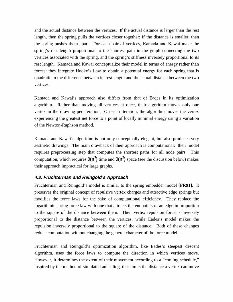
and the actual distance between the vertices. If the actual distance is larger than the rest
length, then the spring pulls the vertices closer together; if the distance is smaller, then
the spring pushes them apart. For each pair of vertices, Kamada and Kawai make the
spring’s rest length proportional to the shortest path in the graph connecting the two
vertices associated with the spring, and the spring’s stiffness inversely proportional to its
rest length. Kamada and Kawai conceptualize their model in terms of energy rather than
forces: they integrate Hooke’s Law to obtain a potential energy for each spring that is
quadratic in the difference between its rest length and the actual distance between the two
vertices.
Kamada and Kawai’s approach also differs from that of Eades in its optimization
algorithm. Rather than moving all vertices at once, their algorithm moves only one
vertex in the drawing per iteration. On each iteration, the algorithm moves the vertex
experiencing the greatest net force to a point of locally minimal energy using a variation
of the Newton-Raphson method.
Kamada and Kawai’s algorithm is not only conceptually elegant, but also produces very
aesthetic drawings. The main drawback of their approach is computational: their model
requires preprocessing step that computes the shortest paths for all node pairs. This
computation, which requires θ(n3) time and θ(n2) space (see the discussion below) makes
their approach impractical for large graphs.
4.3. Fruchterman and Reingold’s Approach
Fruchterman and Reingold’s model is similar to the spring embedder model [FR91]. It
preserves the original concept of repulsive vertex charges and attractive edge springs but
modifies the force laws for the sake of computational efficiency. They replace the
logarithmic spring force law with one that attracts the endpoints of an edge in proportion
to the square of the distance between them. Their vertex repulsion force is inversely
proportional to the distance between the vertices, while Eades’s model makes the
repulsion inversely proportional to the square of the distance. Both of these changes
reduce computation without changing the general character of the force model.
Fruchterman and Reingold’s optimization algorithm, like Eades’s steepest descent
algorithm, uses the force laws to compute the direction in which vertices move.
However, it determines the extent of their movement according to a “cooling schedule,”
inspired by the method of simulated annealing, that limits the distance a vertex can move
as a decreasing function of the number of iterations performed. Frick et al. address the
inefficiency of Fruchterman and Reingold’s cooling schedule by introducing the notion of
local vertex temperatures and also attempting to detect vertex oscillation and rotation of
the entire drawing [FLM94] .
Fruchterman and Reingold claim that the main goals of their approach are speed and
simplicity, and that the main advantage of their approach over others is the former. Like
others, they do not address the problem of drawing large graphs, for which their fixed
number of iterations would be insufficient. All of the examples in their paper, for which
they claim that their algorithm produces drawings in less than ten seconds on a SPARC
station 1, are graphs of under forty vertices. A harsher criticism of their approach,
however, is that the optimization procedure is unnecessarily complicated. The cooling
schedule that they use to determine how much the vertices move on each iteration is a
poor substitute for a line search (which we discuss in Chapter 7); in fact, it can cause their
algorithm to converge to a point that is not locally optimal.
4.4. Models that Address Edge Crossings
The force-directed models described above focus on two aesthetics: keeping edges short
and distributing vertices uniformly throughout the drawing area. In Kamada and Kawai’s
model, one aesthetic summarizes these two: making the distance between vertices
correlate to the lengths of the shortest paths connecting them in the graph. None of these
models, however, takes edge crossings into account.
Two models that consider edge crossings are those of Davidson and Harel [DH96] and of
Tunkelang [Tu94]. Both are energy models that include a term proportional to the
number of edge crossings. Davidson and Harel use a simulated annealing algorithm for
optimization, while Tunkelang uses a collection of local optimization heuristics. The
discreteness of the edge crossing term rules out the continuous optimization methods
used by the other force-directed approaches.
4.5. Computational Complexity
All of the force-directed approaches we have described are iterative. We therefore
consider the computational complexity of performing a single iteration, as well as the
number of iterations necessary to converge to a locally optimal drawing.

For the approaches of Eades, Fruchterman and Reingold, and variations thereof, the cost
of performing an iteration is essentially that of computing the net force acting on every
vertex. In a graph of n vertices and m edges, there are m springs and ½ n (n-1) pairs of
vertices. Hence, the cost of computing all of the forces is θ(n2). The number of
iterations necessary for convergence is poorly understood, but the consensus seems to be
that a steepest descent approach requires a number of iterations that is linear in the
number of vertices. Hence, the overall running time is θ(n3).
Kamada and Kawai’s approach, however, is quite different. Because it only moves one
vertex per iteration, it can recompute the forces incrementally in θ(n) time. The catch,
however, is in the time and space necessary for the preprocessing step of computing all
shortest paths. Kamada and Kawai’s algorithm performs this computation in θ(n3) time,
though this time could be reduced to θ(nm log n) for sparse graphs by executing
Dijkstra’s single-source shortest paths algorithm for each vertex [CLR90] . Even for
sparse graphs, however, storing the computed shortest paths requires θ(n2) space.
Kamada and Kawai claim that the number of iterations necessary for convergence is
linear in the number of vertices. Hence, the overall running time is dominated by the
preprocessing time.
4.6. Other Force-Directed Work
The simplicity of the force-directed approach has invited endless variations, a few of
which we list here. Sugiyama and Misue use “magnetic” springs and fields that try to
make edges conform to particular orientations [SM94]. Ignatowicz uses “orthogonal”
springs to try to make edges meet at right angles [Ig95],. Coleman and Parker apply a
variety of aesthetics to Fruchterman and Reingold’s algorithm [CP96].
Two recent papers incorporate constraints into the spring embedder model. Wang and
Miyamoto introduce absolute constraints on vertex position, constraints that restrict
relative vertex position, and cluster constraints that cause the algorithm to treat subgraphs
independently of each other [WM95] . He and Marriott allow linear constraints, as well
as “suggested values” for vertex positions [HM96] .
4.7. Summary of Problems in Published Approaches
The force-directed approaches of Eades and others cast the graph drawing problem into a
framework of numerical optimization. Unfortunately, they do so without benefiting from
the wealth of knowledge that numerical optimization offers as an established discipline.

Most of the papers of force-directed graph drawing barely even acknowledge that they are
using numerical optimization as a framework. In general, they do not take sufficient
advantage of results from other fields.
The most obvious flaw of the published force-directed algorithms is that they do not scale
gracefully. The ever-increasing speed of hardware cannot keep up with a running time
that is θ(n3), much as cheap memory is not cheap enough for us to use an algorithm that
requires θ(n2) space. Our principle contribution to the field is to apply results from the
fields of numerical optimization and many-body simulation to reduce this asymptotic
running time, as well as to create an approach that meets Fruchterman and Reingold’s
goals of speed and simplicity.

5. Modeling Graph Drawing as an Optimization Problem
In this chapter, we formally describe the force-directed approach for modeling general
graph drawing as a numerical optimization problem.
5.1. Output Variables
We denote the input graph by G. G consists of the vertex set V = v1, v2, …, vn and the
edge set E = e1, e2, …, em. We denote the two endpoints of an edge e by from(e)
and to(e) . Since our edges are undirected, the ordering of the endpoints is arbitrary.
We will assume for the next few chapters that all vertices are mapped to dimensionless
points and all edges to straight line segments connecting their endpoints. While we
primarily intend our model for drawings in the plane, the model applies without
modification to drawings in higher dimensional spaces.
We define the output variables x(vi)—or xi for short—to be the position vectors of
vertices vi, for i equal to 1, 2, …, n. For a given graph G, we denote a drawing D by the
n-dimensional vector of vectors [x1, x2, …xn]. Because the edges are straight line
segments, the drawing of G is completely specified by this vector of vertex positions.
5.2. Force Laws
As we described in the previous chapter, the force-directed approach models graph
drawing using a physical analogy. We use a force model in which our force laws produce
a vector that is the negative gradient of an implicit energy function we seek to minimize.
There are force laws corresponding to different aesthetic criteria:
Springs. We associate a spring with each edge. A spring pulls the endpoints of the edge
it represents towards each other when their distance exceeds the spring’s rest length and
pushes them away from each other when their distance is smaller than the rest length. If
the rest length is zero, then the spring always pulls the endpoints towards each other.
Vertex-vertex repulsion. All vertices push each other away in order to avoid overlap
among vertices and to spread the vertices out uniformly throughout the drawing area.
The magnitude of this repulsion force for a given pair of distinct vertices is a decreasing
function of the distance between the two vertices.

Vertex-edge repulsion. Vertex-vertex repulsion may not prevent a vertex from being
placed so close to an edge—possibly overlapping it—that the edge appears to be incident
to the vertex. Hence, we include a term in the force model for every vertex-edge pair;
again, the magnitude is a decreasing function of the distance between the vertex and edge.
Although we will refer to the energy of a drawing when we discuss the numerical
optimization procedure, we will mostly discuss the negative gradient of the objective
function, which is the vector corresponding to the net forces on all of the vertices.
5.2.1. Springs
Since the edges specify which vertex pairs have a direct relationship, the corresponding
springs serve to exhibit the importance of these relationships in the drawing.
The simplest of spring laws is Hooke’s Law with a rest length of zero. Using Hooke’s
Law for the springs gives us, for edge ei, a force of magnitude kx attracting each endpoint
towards the other, where x = ||x(from(e i)) - x(to(e i))|| and k is a constant representing
the stiffness of the springs. We could assign a different stiffness ki to each edge ei to
reflect the relative importance of each edge; the stiffer springs would correlate in smaller
edges in an optimal drawing.
Hooke’s Law (with a rest length of zero) is computationally appealing because the force
vector can be computed using only one vector subtraction and one scalar multiplication.
In fact, if the coordinates and spring constant(s) are integers, then the force vector can be
computed exactly using only integer arithmetic.
Fruchterman and Reingold, however, found that they had more success using a quadratic
spring force—that is, a force of magnitude proportional to ||x(from(e i)) - x(to(e i))||2.
We will discuss the constant of proportionality in a moment.
Fruchterman and Reingold observed that a linear spring force is often not strong enough
to overcome poor local minima—that is, local minima in the objective function that are
far inferior to the global minimum. Hence, they were willing to incur the additional
arithmetic operations (which include a square root) necessary for a quadratic spring force.
They also experimented with using higher order powers for the spring force, but rejected
them on the grounds that the were more costly to compute. In fact, a cubic spring force

would be less expensive to compute than a quadratic force, since it does not require
computing a square root. We did find, however, that using higher order powers for the
spring force slows down our optimization procedure by making the force laws less
smooth.
Eades’s original spring force for the spring embedder model was logarithmic, the
magnitude of the force being proportional to log(|| x(from(e i)) - x(to(e i))|| / x0), where
x0 is a user-specified constant. A fact that Eades does not mention is that this spring
force becomes repulsive (rather than attractive) when ||x(from(e i)) - x(to(e i))|| < x0.
Regardless of this short-range behavior, we found, as we discussed earlier, that a
logarithmic spring force leads to an unaesthetically high degree of variance in the edge
lengths.
Kamada and Kawai use an model that relies exclusively on springs. Instead of only
associating springs with the edges, they associate a spring with every pair of distinct
vertices. Their springs conform to Hooke’s Law; the rest length and stiffness of each
spring depend on the length of the shortest path in the graph connecting the two vertices.
If the shortest path connecting vi and vj has a length of shortestPath(v i, vj) edges, then
the rest length of the corresponding spring is proportional to shortestPath(v i, vj), while
the stiffness is proportional to 1/shortestPath(v i, vj). In other words, the magnitude of
the spring force that each pair of distinct vertices (vi, vj) exert on each other is
proportional to (1 / shortestPath(v i, vj)) • | ||xi - xj|| - c • shortestPath(v i, vj) |,
where the constant c reflects the desired length of an edge. As Kamada and Kawai note,
their model applies to graphs with either unit edges or weighted edges; in the latter case,
shortestPath(v i, vj) denotes the sum of weights along the shortest path connecting
distinct vertices vi and vj.
As we noted in the previous chapter, Kamada and Kawai’s model relies on a time and
space-intensive pre-processing phase to compute and store the θ(n2) shortest path lengths.
Moreover, as we will see later, associating springs with all vertex pairs prevents us from
using many-body simulation methods to reduce computation. Hence, we stick to a model
of springs and repulsion.
Our own experiments agree with Fruchterman and Reingold’s observation that quadratic
spring force laws work better than linear springs to avoid poor local minima, and we
found that using higher order polynomials for the spring laws slowed down our

optimization procedure. We therefore use Fruchterman and Reingold’s quadratic spring
law. In Chapter 9, we describe a modification to this law that takes vertex shape and size
into account.
5.2.2. Vertex-Vertex Repulsion
If our objective function consisted only of springs of rest length zero, then the globally
optimal drawing would assign all vertices to a single point. Making the rest lengths non-
zero would ameliorate the situation somewhat, but edge springs alone are insufficient to
produce an acceptable drawing. For example, let us consider the three-vertex path where
V = 1, 2, 3 and E = (1, 2), (2, 3) . A globally optimal drawing would space the
vertices uniformly along a line. In the absence of a force that involves vertices 1 and 3,
these two vertices could even be assigned to identical coordinates.
As we have discussed, we reject Kamada and Kawai’s solution of springs for all node
pairs because of the impractical time and space requirements of the preprocessing step.
Instead, we introduce vertex-vertex repulsion terms into the physical model.
In Eades’s force model, vertices repel each other as if they were like-charged particles
acting in accordance with Coulomb’s inverse-square law. Every pair of distinct vertices
vi and vj repel each other with a force whose magnitude is proportional to 1/||xi - xj||2.
When two vertices have identical coordinates, the magnitude of the repulsion force goes
to infinity. We therefore disallow assignment of distinct vertices to identical coordinates.
If we ever encounter a drawing where this situation occurs, we randomly separate the
coincident vertices by a small distance.
Fruchterman and Reingold, concerned with reducing the number of arithmetic operations
per repulsion computation and preferring to avoid taking square roots, use a force law that
is inverse rather than inverse square. The magnitude of the repulsion force in their model
is proportional to 1/||xi - xj||.
Now, we can discuss the constants of proportionality in Fruchterman and Reingold’s
model. Fruchterman and Reingold define the constant k to denote the rest length of an
edge. They choose their constants of proportionality for the spring and repulsion laws so
that, when the length of an edge is k, then the spring and vertex-vertex repulsion forces
exerted by the endpoints cancel out. In other words, two vertices joined by an edge, in

the absence of additional forces exerted on them, exert no net force when the distance
between them is exactly k. When they are closer, the repulsion is stronger than the spring
and pushes them apart; when they are further, the spring is stronger and pulls them
towards each other.
The constants of proportionality are 1/k for the quadratic spring force and k2 for the
inverse vertex-vertex repulsion force. When the two endpoints of an edge are distance k
apart, both forces have magnitudes of k and cancel each other out.
One issue that receives little attention in the force-directed graph drawing literature is that
vertex-vertex repulsion forces serve two distinct purposes. One is to avoid vertex
overlap. It is not enough that vertices be assigned distinct coordinates; since vertices are
generally drawn as rectangles or ellipses with information inside them, it is preferable that
they be drawn far enough apart from each other to be legible. The other purpose is to
distribute vertices uniformly throughout the drawing space. This second goal is quite
different from the first, and is generally a lower priority that has more to do with
aesthetics—e.g., display of symmetry—than with legibility.
While the magnitude of the vertex-vertex repulsion force does decrease as a function of
the distance between the vertices, the long-range effects of an inverse force law like that
of Fruchterman and Reingold can be too strong, resulting in pockets of undesirably high
local density. We therefore split the vertex-vertex repulsion force into a stronger short-
range force and a weaker long-range force. When the distance between two vertices is
less than k, we use an inverse repulsion law; when the distance exceeds k, we use a
weaker inverse-square law. In order to achieve computational stability, we make the
magnitude of the repulsion force continuous at k.
This way of splitting the forces is admittedly inelegant, but is a first step towards adapting
the concept of vertex-vertex repulsion to address the distinct issues of avoid vertex
overlap and distributing vertices uniformly.
We use the same constants of proportionality as Fruchterman and Reingold for the spring
forces (1/k) and the short-range inverse repulsion (k2). To achieve continuity, we use a
constant of k3 for our long-range inverse-square repulsion law.

In Chapter 9, we will discuss how node shape and size affect the vertex-vertex repulsion
law. In Chapter 8, we will also discuss the computational consequences of choosing a
weaker or stronger repulsion law, and how we can use a time-dependent gradient to
improve performance.
5.2.3. Vertex-Edge Repulsion
In the force-directed models we have discussed, all of the forces involve vertex pairs.
Sometimes these forces allow a vertex to be very close to an edge. When an edge is
short, then the vertex-vertex repulsion will probably push vertices away from it. When an
edge is long, however, the vertex-vertex repulsion may not prevent a vertex from being
very near the edge, since it can do so without being that close to either of the endpoints.
Our concern is with vertex-edge overlap. If a vertex overlaps an edge or is placed very
close to it, then it becomes difficult or impossible to determine if the edge is incident to
that vertex. Hence, we need a strong short-range vertex-edge repulsion term to avoid this
situation. Since we are not using vertex-edge repulsion to spread out the vertices
uniformly, we do not need the force to be long-range at all. We do, however, need to
make the repulsion force continuous so that we have computational stability.
We consider two cases for vertex-edge repulsion. In the first case, the point on the edge
closest to the vertex is one of the endpoints. In the second case, the point closest to the
vertex lies strictly between the endpoints.
In the first case, our vertex-edge repulsion force acts much like the short-range inverse
vertex-vertex repulsion force acting on the vertex and the endpoint nearest to it. The only
difference is that, in order to make the vertex-edge repulsion force both short-range and
continuous, we subtract k from the magnitude of the force. Accordingly, the magnitude
of the force is cve((k2/x) - k) when x, the distance between the vertex and the closer
endpoint, is less than k (we will discuss cve in a moment). This force pushes the vertex
and the endpoint closest to it away from each other; it does not affect the further endpoint.
Indeed, it only amplifies the vertex-vertex repulsion force that the two vertices already
exert on each other. We need this force, however, to ensure continuity with the second
case.
The second case is more complicated. First, we compute the distance x between the
vertex on the edge by projecting the former onto the latter. Let us denote the vertex by v,

the edge by e, and the projection of v onto e (that is, the point on the edge closest to v) by
p. Let α = ||p - x(from(e))|| / || x(to(e i) - x(from(e i))||. By assumption, α ∈ [0, 1] ;
the boundary situations (α = 0, α = 1) represent the first case, where the point on the
edge close to v is an endpoint.
We can now describe the vertex-edge repulsion force law for the second case. Vertices v
and from(e) repel each other with a force of magnitude (1-α)cve((k2/x)-k) .
Symmetrically, vertices v and to(e) repel with a force of magnitude (α)cve((k2/x)-k) . As
we can see by setting α to 0 or 1, the boundary cases are continuous.
The constant cve is a non-negative weight that reflects the priority of avoiding vertex-
edge overlap. We have found that a small value of cve works well; our own
implementation sets it to 0.1.
5.3. Constraints
Constraints can be either equalities or inequalities in the output variables. A drawing that
satisfies all of its constraints C1, C2,… is said to be feasible, and the set of such drawings
is said to be the feasible space of drawings. If the set of constraints is empty, then all
drawings are feasible, and the problem is said to be unconstrained.
5.3.1. Penalty Functions
For every constraint Ci, we will require an associated penalty function pi that measures
the distance of a drawing to the nearest drawing that satisfies Ci. We can define such
penalty functions for both equality and inequality constraints. The requirement that these
penalty functions exist allows us to use the method of exterior penalties to perform
constrained optimization. We will describe this method in Chapter 8.
5.3.2. Constraints versus Preferences
It is often possible to quantify aesthetic criteria either as constraints or as terms in the
objective function. In the latter case, the criteria become preferences that are combined
and prioritized according to their relative weights. The choice of whether to represent an
aesthetic criterion with constraints or preferences is key to the modeling problem, so we
will discuss the advantages and disadvantages of each type of formulation.
For example, we may have two vertices that are very strongly related. A simple way to
express the strength of their relationship in the drawing is to constrain them to lie within a

certain distance of each another. Alternatively, we could represent this strength using a
spring term in the objective function with a high spring constant.
The main advantage of constraints is their simplicity. If we have non-negotiable aesthetic
criteria and can express them as boolean predicates, then constraints provide a
straightforward mechanism for doing so. Typical constraints address minimal separation
between nodes, drawing boundaries, clustering, and edge direction.
Constraints, however, have two major disadvantages. First, their binary nature limits
their expressiveness. In the example above, we can use constraints to specify a minimum
node separation, but our formulation does not favor larger distances over small ones. The
second problem is more serious: they generally add complexity to the optimization
process and thus slow it down. Here, we must accept that there is a trade-off between
speed and flexibility.

6. Computing the Gradient Efficiently
The θ(n3) running time of most of the published graph drawing algorithms effectively
limits their domain to very small graphs. To draw larger graphs, we must dramatically
reduce the running time.
In this chapter, we focus on making the computation of the gradient as efficient as
possible. In particular, we attack the bottleneck of the published force-directed
approaches—the θ(n2) computation of repulsion forces. After discussing two simple but
problematic methods that reduce this computation to θ(n), we discuss more sophisticated
approaches drawn from the many-body simulation literature.
6.1. Computing the Gradient Naïvely
In order to compute the gradient of a drawing as we defined it in the previous chapter, we
need to take a sum of θ(m) spring forces, θ(n2) vertex-vertex repulsion forces, and
θ(nm) vertex-edge repulsion forces. Even without considering vertex-edge repulsion
forces, we would require θ(n2) time to compute the gradient straightforwardly—that is,
by summing all of the spring and vertex-vertex repulsion forces to compute the net force
acting on each vertex.
A running time of θ(n2) or θ(nm) for a single gradient computation severely limits the
size of graphs that we can draw. For dense graphs—that is, where m is θ(n2)—we have
little hope of doing better unless we can somehow summarize the graph in a smaller
representation. For example, we could take a divide-and-conquer approach that partitions
the vertices into subsets, draws each subset independently, and then draws the graph of
subsets as if each subset were a single large vertex. This partitioning problem, however,
is beyond the scope of this dissertation. We thus assume we cannot avoid computing the
spring forces, and this computation requires θ(m) time.
For sparse graphs, however, there is a wide gap between θ(m) and θ(n2). Indeed, for
sparse graphs, we spend most of the computation on the repulsion forces—that is,
assuming that we compute these forces naively. Accordingly, we devote our efforts to
computing these repulsion forces more efficiently.

6.2. Simple θ(n) Approximations for Computing Vertex-Vertex Repulsion
In the force-directed graph drawing literature, two techniques appear for approximating
the computation of the vertex-vertex repulsion forces. Fruchterman and Reingold
describe a “grid variant” of their algorithm that ignores repulsion forces between vertex
pairs whose distance exceeds a threshold of 2k, using an auxiliary grid structure to reduce
computation. As we discussed in the previous chapter, k is the rest length of an edge—
that is, the distance at which the two endpoints of an edge exert no net force on each other
because the spring and repulsion forces cancel out. Fruchterman and Reingold claim that
this approximation produces drawings that are “nearly equivalent” to those obtained
without approximation. They note that this approximation of the repulsion forces has a
running time that is θ(n) when the vertex distribution in the drawing area is
“approximately uniform”; the efficiency of their grid structure depends on the uniformity
of the distribution. Coleman and Parker suggest the alternative approach of “centripetal
repulsion”—that is, repulsion from the centroid of the drawing. The cost of this
approximation is θ(n) time (and no additional space) regardless of the distribution of
vertices.
6.2.1. Distance Cut-Offs
Distance cut-offs are a conceptually simple approach to approximating vertex-vertex
repulsion. Since the magnitude of the vertex-vertex repulsion forces decays rapidly with
distance between the two vertices, we can ignore repulsion between far-away vertices
and only incur a small additive error in the gradient. Moreover, we can implement
distance cut-offs, as Fruchterman and Reingold do, with a straightforward data-structure:
we partition the drawing space uniformly into a grid of square cells where the side of each
square is the cut-off distance. Fruchterman and Reingold choose their constants so that
k2n is proportional to the area of the drawing space, making the number of grid cells—
and hence the additional space required for the grid—θ(n).
We can easily determine a bound on the maximum additive error caused by using
distance cut-offs. In Fruchterman and Reingold’s force model, the magnitude of the
repulsion force between nodes vi and vj is k2 / ||xi - xj||. When ||xi - xj|| = 2k , this force
has a magnitude of k/2. Hence, the maximum additive error in computing the magnitude
of each repulsion force is k/2.
While the additive error resulting from distance cut-offs is small, they are unsatisfactory
for two reasons. The first is basic: by ignoring long-distance repulsion forces, we inhibit

most of the effect that vertex-vertex repulsion would normally have in distributing the
vertices uniformly throughout the drawing space. The second is that distance cut-offs
cause problems for the optimization procedure. In Fruchterman and Reingold’s model,
the cut-offs make the force model discontinuous wherever the the distance between two
vertices is exactly 2k, since the magnitude of the repulsion force jumps from k/2 to 0.
Such discontinuities can cause a optimization procdure to oscillate around them. We can
remove the discontinuties using the technique we applied to our short-range vertex-edge
repulsion force—that is, we can make the magnitude of the vertex-vertex repulsion force
k2 / ||xi - xj|| - k/2 so that it is continuous at ||xi - xj|| = 2k . Fruchterman and Reingold’s
algorithm handles the discontinuties by dampening forces using a “cooling schedule”, but
there is no guarantee that the drawing to which it converges will be locally optimal.
We can lessen the consequences of distance cut-offs by increasing the cut-off distance.
Assuming that the graph is connected, there always exists a cut-off distance that has no
effect on the objective function—namely, any value greater than the diameter of the
optimal drawing. Doing so, however, defeats the entire purpose of the approximation,
which is to reduce computation.
Indeed, the efficiency of Fruchterman and Reingold’s grid variant hinges on the
assumption that the number of vertices within the cut-off radius of a vertex is, on average,
θ(1). If we further assume a uniform distribution of vertices in the drawing space, then
this requirement implies a θ(k) cut-off distance, since the expected number of vertices
within a cut-off radius of r is θ(r2/k2). As a result, modifying the grid variant to use a
cut-off distance of r increases the running time (assuming uniform vertex distribution) to
approximately compute repulsion forces from θ(n) to θ(r2n/k2), where r is at most
O(k n ). If r is greater, then we may as well use the naïve θ(n2) approach.
The assumption that the vertex distribution will be “approximately uniform” is, however,
somewhat questionable. As shown in Figure 6.1, a cycle of n vertices with edges of
length k requires a drawing area of θ(k2n2) to be drawn as a regular polygon—which is
accepted as the optimal way to draw an undirected cycle. Fruchterman and Reingold’s
grid variant can handle this situation in a few ways. One possibility is to impose a
drawing space of area θ(k2n), in which case the boundary will severely constrain the
drawing. If the area of drawing space is θ(k2n2), then there is the question of choosing
the number of grid cells. If there are θ(n) grid cells, then, as the drawing approaches its
optimum, each of the θ( n ) cells on the perimeter will contain θ( n ) vertices, making the
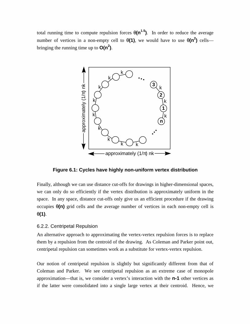
total running time to compute repulsion forces θ(n1.5). In order to reduce the average
number of vertices in a non-empty cell to θ(1), we would have to use θ(n2) cells—
bringing the running time up to O(n2).
1
2
3
n
...
...
k
k
k
kk
k
k
k
k
k
kk
approximately (1/π) nk
appr
oxim
atel
y (1
/π)
nk
Figure 6.1: Cycles have highly non-uniform vertex distribution
Finally, although we can use distance cut-offs for drawings in higher-dimensional spaces,
we can only do so efficiently if the vertex distribution is approximately uniform in the
space. In any space, distance cut-offs only give us an efficient procedure if the drawing
occupies θ(n) grid cells and the average number of vertices in each non-empty cell is
θ(1).
6.2.2. Centripetal Repulsion
An alternative approach to approximating the vertex-vertex repulsion forces is to replace
them by a repulsion from the centroid of the drawing. As Coleman and Parker point out,
centripetal repulsion can sometimes work as a substitute for vertex-vertex repulsion.
Our notion of centripetal repulsion is slightly but significantly different from that of
Coleman and Parker. We see centripetal repulsion as an extreme case of monopole
approximation—that is, we consider a vertex’s interaction with the n-1 other vertices as
if the latter were consolidated into a single large vertex at their centroid. Hence, we

modify Coleman and Parker’s approach in two ways. First, vertices experience repulsion
from the centroid of the n-1 other vertices, rather than from the centroid of all n vertices
in the drawing. Second, the repulsion force is mutual—that is, the centroids are also
repelled by the vertices. This latter modification ensures that the sum of all repulsion
force vectors in the drawing always cancels out, and hence that the centroid of the
drawing will not drift. Like distance cut-offs, centripetal repulsion generalizes to
drawings in higher dimensional spaces.
Centripetal repulsion has several immediate advantages over distance cut-offs. The time
necessary to compute all of the centripetal repulsion forces is θ(n) regardless of the
vertex distribution, and there is no need to maintain an auxiliary grid data structure.
Centripetal repulsion does not suffer from the discontinuities of distance cut-offs; in fact,
the further a vertex is from the centroid of its neighbors, the more accurate the
approximation. Also, for drawings in higher dimensional spaces, the cost of computing
centripetal repulsion only increases linearly with the number of dimensions. Indeed, it is
a more elegant model, both in concept and in the implementation.
Unfortunately, its inaccuracy can be far more severe than that of distance cut-offs. Let us
consider the 15-vertex binary tree drawn optimally in Figure 6.2. Using centripetal
repulsion, we obtain the bizarre drawing in Figure 6.3. Because vertices don’t repel each
other directly, it is even possible for them to be assigned to identical coordinates. A
smaller but still significant problem with centripetal repulsion is that it distorts the
drawing near its centroid.
1 3
7
15
14
6
12
13
2
5
11
10
4
8
9
Figure 6.2: Optimal Drawing of Tree

13 6,72
8-114,5
12-15
Figure 6.3: Same Tree Drawn using Centripetal Repulsion
We might address this problem by combining distance cut-offs with centripetal repulsion,
but this approach would be messy. It would also suffer from the problems of both
approaches—for example, degradation in speed when the vertex distribution is not close
to uniform, and distortion near the centroid. Instead, we turn to the many-body
simulation literature for a better solution.
Interestingly, the two approaches we have discussed, distance cut-offs and centripetal
repulsion, demonstrate the two distinct purposes of the vertex-vertex repulsion force.
Distance cut-offs focus only on the short-range repulsion for avoiding overlap, while
centripetal repulsion helps make the vertex distribution more uniform. As we will see,
we can accomplish both of these goals by combining our distinction between short- and
long-range repulsion with an efficient tree-code.
6.3. Approximating Vertex-Vertex Repulsion Forces in θ(n log n) Time
The problem of computing the pair-wise interactions among a large collection of particles
is a familiar one to physicists. Indeed, their methods for approximating gravitational and
electrostatic forces are directly relevant to our problem.
Two popular procedures to compute this approximation are Greengard and Rokhlin’s Fast
Multipole Method (FMM) [GR87] and the Barnes-Hut algorithm [BH86]. Both rely on
partitioning the set of particles hierarchically into a tree of cells. Barnes-Hut replaces
most particle-particle interactions with particle-cell interactions, while FMM computes a
series of cell-cell interactions. Although worst-case running-time of FMM is
asymptotically better than that of Barnes-Hut—θ(n) versus θ(n log n) —it has much
more overhead and is also more complicated to implement. The performance and
accuracy of Barnes-Hut are more than adequate for our purposes.
We now describe how the Barnes-Hut algorithm works for particles in two dimensions.
The algorithm consists of two phases. In the first, we partition the drawing space by
creating a quad-tree of rectangular cells. In the second, we traverse the quad-tree to

approximate the net force acting on each particle. The algorithm generalizes to spaces of
higher dimension, and is commonly applied to problems in three dimensions.
6.3.1. Building the Quad-Tree
In the first phase, we insert all of the particles into a quad-tree. A quad-tree is a
hierarchical partitioning of a rectangle, where each internal node of the tree represents a
rectangle that has been split into four congruent subrectangles (i.e. bisected horizontally
and vertically) and each leaf is an undivided rectangle. We refer to both internal nodes
and leaves of the quad-tree as cells.
We begin with a single empty cell that represents the bounding rectangle of the particles.
If we do not already know the bounding rectangle, we can compute it in θ(n) time, where
n is the number of particles.
We then insert the particles into the quad-tree sequentially. When we insert a particle, we
begin at the root of the quad-tree. We increment the number of particles stored in that
cell by one, and also update that cell’s centroid. If the cell was empty, then its centroid is
the position of the inserted particle; otherwise, we take a weighted average of the
previous centroid and the new particle’s position. Now there are three cases. If the cell
was an empty leaf, then we are done with the insertion. If the cell is an internal node, we
recursively insert the particle into the subcell corresponding to the rectangle that contains
the particle. If the cell was a leaf that already had a particle in it, then we make the cell an
internal node, splitting it into four subcells. We then recursively insert both of the cell’s
particles into the appropriate subcells.
Figure 6.4 illustrates how we partition the bounding rectangle of the particles into cells
such that each cell contains at most one particle. Figure 6.5 shows a quad-tree that
represents this partitioning. The children of a cell represent, in order, the northwest,
northeast, southwest, and southeast quadrants of that cell.
Our insertion procedure maps each particle to a unique leaf in the quad-tree. There are
also empty leaves in the tree—possibly as many as three for each internal node of the tree.
In total, the space requirement for the quad-tree is θ(n).
The time required to create the quad-tree depends on its height. Inserting a particle
requires time proportional the distance from the root to the leaf that contains that particle.

We note that, even if a subsequent insertion moves the particle further down the tree, the
total time spent on inserting that particle is still proportional to its ultimate distance from
the root. Hence, the total time spent on creating the quad-tree is proportional to the sum
of the heights of its leaves.
1 23
45
67
8
9
1011
12
13
14
15
Figure 6.4: Partitioning the Bounding Rectangle into Cells
2 4
3
1 8 10
NW NE SW SE
14
12 13 155 9
6 7 11
Figure 6.5: A Quad-Tree Representing the Partitioning
Clearly, the height of the quad-tree has a lower bound of Ω(log n) , giving us a
corresponding lower bound of Ω(n log n) for creating the tree. We could, however,
have a quad-tree of arbitrary height h, and such a tree would require θ(nh) time to create.
Such a highly imbalanced tree, however, imply that the smallest distance between two
particles was O(2-hs), where s is the length of the longer side of the bounding rectangle
of the particles. We are not, however, dealing with an arbitrary distribution of particles in
space. Because we are dealing with graph drawing, we can reasonably assume that there

is a constant lower bound on the smallest distance between particles. We can also assume
that s is O(n), the bounding case being a path of n vertices drawn along a straight line.
Hence, each leaf has an area that is at least Ω(1/n) fraction of the area of the bounding
rectangle. This lower bound implies that the height of the quad-tree is O(log n) , making
the time to create it θ(n log n) .
6.3.2. Computing the Force on Each Particle
The performance gain in the Barnes-Hut algorithm comes from computing the force
exerted on a particle by other far-away particles with a monopole approximation—that is,
treating collections of particles as if they were clustered at their centroids. We do have to
take care, however, not to make gross errors using this monopole approximation.
The procedure for computing the force acting on a particle works as follows. We first
find the leaf cell of the quad-tree associated with that particle. We then compute the force
exerted by each of that cell’s siblings on the particle. When then take the leaf’s parent in
the tree and compute the force exerted by each of the parent’s siblings on the particle.
We do the same with the parent’s parent, and so forth, until we reach the root.
How we compute the force that a cell exerts on the particle depends on whether the leaf
cell containing the particle is well separated from the cell. Barnes and Hut define this
concept as follows: a particle and a cell are well separated if the ratio r/D is less than θ,
where r is the length of a side of the cell, D is the distance between the particle and the
centroid of the cell, and θ is a fixed accuracy parameter between zero and one. We will
discuss the choice of θ in a moment.
If a particle is well separated from a cell, then we compute the force exerted by the cell as
if all of its particles were located at the centroid of the cell. Otherwise, we recursively
compute the force exerted by each of the subcells of that cell on the particle.
The reason for insisting that cells be well separated for the monopole approximation is
that using centroids for cells that are not well separated can result in unbounded errors.
Two particles that are very close to each other may end up in leaf cells that share a border
but are nonetheless far apart from each other in the quad-tree.
Barnes and Hut suggest setting θ to be approximately 1. Salmon has shown the total
number of force computations necessary is O(θ-3 n log n) [Sa90], and that the errors in

the force computation can be unbounded if θ ≥ d-½, where d is the number of dimensions
of the space [SW94]. If d = 2, we must pick θ < 0.707. We have had good results with
θ = 0.7 is more than sufficient. In particular, our algorithm does not suffer from the
discontinuities introduced by reorganizing the quadtree as vertices move in the drawing.
We should note that the above error analysis assumes that the force law is an inverse-
square law, as is the case in gravitation and electrostatics. In practice, we have found that
the Barnes-Hut algorithm works even when the force law is inverse. In any case, our
long-range repulsion force is inverse-square.
We conclude this section with an example: we use the Barnes-Hut algorithm to compute
the force acting on particle 1 in Figure 6.4.
The siblings of the associated leaf cell are the leaf cell containing particle 8; the non-leaf
cell containing particles 2, 3, and 4; and the leaf cell containing particle 10. The
computation is trivial for the two siblings that are leaves; we just compute the ordinary
particle-particle forces.
The non-leaf sibling requires more work. Since it is not well separated from the leaf cell
containing particle 1, we have to compute the forces that its children exert on particle 1.
The non-empty children are the non-leaf cell containing particles 2 and 4, and the leaf
cell containing particle 3. Again, the leaf cell computation is trivial, but again the non-
leaf cell is not well-separated from the leaf containing particle 1. Hence, we look at its
non-empty children, which are both leaves.
Now, we look at the siblings of the parent of the leaf cell containing particle 1. These are
the non-leaf cell containing particles 5, 6, 7, 9, and 11; the leaf cell containing particle
14; and the non-leaf cell containing particles 12, 13, and 15. Finally, we see how the
quad-tree helps: both of the non-leaf cells are well separated from the leaf cell containing
particle 1. Hence, we compute the force that each exerts in constant time by treating each
cell as if all of its particles were at its centroid.
Since the parent of the parent of the leaf cell containing particle 1 is the root of the quad-
tree, we are done.

6.3.3. Applying Barnes-Hut to Compute Vertex-Vertex Repulsion Forces
The vertex-vertex repulsion in our physical model considers a particle system like those
that Barnes and Hut had in mind for their algorithm. Our force law does not correspond
exactly to the physical laws of gravitation or electrostatics; nonetheless, the Barnes-Hut
algorithm works very well to approximate it.
We do however, make one minor modification. As we discussed in the context of
centripetal repulsion, we would like the net force on the centroid of the drawing to be
zero, since all of the forces should cancel each other out. Unfortunately, the Barnes-Hut
algorithm does not make us such a guarantee. We address this problem much the way we
did for centripetal repulsion: we make all forces mutual. In other words, a particle exerts
a repulsion force on a cell equal in magnitude to the force that the cell exerts on the
vertex. If the cell contains c vertices, then each of the vertices experiences 1/c of this
force.
6.4. Computing Vertex-Edge Repulsion Forces
We could also modify the Barnes-Hut algorithm to compute vertex-edge repulsion. The
modifications, however, would not be trivial: we would have to break up the line
segments representing edges into sub-segments such that each leaf cell of the quad-tree
would contain at most one sub-segment. The quad-tree would require a space
proportional to the number of sub-segments, which could be somewhat larger than the
number of edges. In addition, we would have to take more care with the force
computation, since the three cases for vertex-edge repulsion are more complicated than
the single law for vertex-vertex repulsion.
A key difference, however, between vertex-vertex and vertex-edge repulsion is that the
latter is a purely short-range force. Using Barnes-Hut is overkill, since we lose no
accuracy by ignoring vertex-edge pairs that are far apart. In fact, we can use distance cut-
offs, taking an approach based on Fruchterman and Reingold’s grid variant.
Like Fruchterman and Reingold, we partition the bounding rectangle of the drawing space
into a grid of square cells such that the side of each cell is k and store in each cell a list of
the vertices it contains. If the vertex distribution is sufficiently uniform, then the number
of cells will be proportional to the number of vertices; otherwise, we can use a sparse
matrix representation in which non-empty cells do not take up memory.

Once we have computed the grid, we iterate over the edges, computing the repulsion
force between it and the vertices that are near it. An edge may not be entirely contained
in one cell, in which case we have to iterate over all of the cells it occupies. Indeed, the
vertices we have to consider are precisely those that are either in the cells occupied by the
edge or are in cells that border those occupied by the edge. If an edge is of length O(k),
then it will occupy O(1) cells.
Unlike Fruchterman and Reingold, we do not have to contend with the inaccuracy caused
by using distance cut-offs. Our vertex-edge repulsion force is short-range by design, so
there is no inaccuracy.
We do, however, suffer the same performance problems that they do if the vertex
distribution is highly non-uniform. One heuristic to address this issue is to ignore vertex-
edge repulsion in the early iterations. By doing so, we solve several problems. By the
time we start computing vertex-edge repulsion, the vertex distribution corresponds
roughly to what it will be in the final drawing. Waiting until later iterations to introduce
vertex-edge repulsion also helps us avoid poor local minima. If, after a large number of
iterations, there are still edges with large numbers of vertices within distance k of them,
then we must resign ourselves to the fact that the drawing is dense and requires more
work. In practice, the number of vertices within distance k of an edge is O(1), making
the time to compute vertex-edge repulsion forces O(m).

7. The Optimization Procedure
So far, we have concerned ourselves only with the efficiency of computing the gradient.
The other factor that determines performance is the number of gradient computations that
our optimization procedure must perform before converging to a local minimum.
As we discussed in Chapter 4, we can think of the graph drawing problem in terms of
either a force model or an energy model. In the previous chapter, we opted for the
former, describing how we encapsulate the aesthetic criteria with force laws. Now it
proves convenient to imagine the sum of these force vectors as the negative gradient of an
energy function that we are trying to minimize. We refer to this implicit energy function
as the objective function.
We restrict our attention to first-order continuous optimization procedures. Such
procedures are iterative: on each iteration, they improve the drawing (which is a vector in
R2n for two-dimensional drawings), translating it by some vector p ∈ R2n. We break
down the problem of computing this vector into two sub-problems: that of choosing a
search direction—that is, the orientation of p—and that of determining the step size, the
magnitude of p.
The algorithms of Eades and of Fruchterman and Reingold use variations of the method
of steepest descent. Accordingly, we first discuss this straightforward method for
choosing the search direction. We then describe how to compute the search direction
using the conjugate gradient method. Finally, we discuss the problem of computing the
step size.
7.1. The Method of Steepest Descent
The method of steepest descent, also known as Euler’s Method in the context of solving
differential equations, uses the negative gradient as the search direction. In the context of
force-directed graph drawing algorithms, moving along the negative gradient simply
means moving each vertex in the direction of the net force exerted on it.
Eades’s optimization procedure uses the method of steepest descent as is. Fruchterman
and Reingold start by computing the negative gradient, but then, instead of computing a
step size, they truncate each vertex’s components of the search direction independently in

order to limit the maximum distance that a vertex can move on that iteration. They
determine this maximum distance according to a “temperature” that is a decreasing
function of the number of iterations performed thus far.
The main selling point of the method of steepest descent is its simplicity. It allows us to
compute a search direction with only one gradient computation. Moreover, as long as we
take some care in choosing the step size and have sufficient numerical precision, the
method of steepest descent will always converge to a local minimum, regardless of our
starting point.
Unfortunately, although the method of steepest descent does eventually converge to a
local minimum, it may take a large number of iterations to do so. We can make this
statement more formally for the case that the objective function is quadratic and positive
definite—that is, its Hessian matrix of second derivatives is constant and has only
positive eigenvalues. In this case, the method of steepest descent is only guaranteed to
converge at a rate that is linear in the condition number of the Hessian, which is defined
as the ratio between the smallest and largest of its eigenvalues. We refer the reader to
Gill, Murray, and Wright [GMW81] for a thorough analysis of the convergence rate of
the method of steepest descent.
In our own case, the objective function is neither quadratic nor positive definite;
nonetheless, the method of steepest descent slows down when the condition number of
the Hessian is large.
By always following the negative gradient, the method of steepest descent models the
local behavior of the objective function as linear. Since non-degenerate linear functions
do not even have local minima, this model is obviously a crude one. While the method of
steepest descent performs reasonably well when we are far away from a local minimum—
where the objective function behaves most linearly—its performance degrades rapidly as
we approach the local minimum.
Often, the method of steepest descent will find itself stuck in a “trough,” a situation we
depict in Figure 7.1. The little black arrows in the figure indicate the direction of the
negative gradient, which each of the thick gray arrows indicates the progress on a single
iteration. Let us assume that we are using the maximum possible step size that will

decrease the objective function. In that case, the method of steepest descent will bounce
back and forth, making very slow progress.
In order to do better than the method of steepest descent, we need a more sophisticated
model of the objective function.
Figure 7.1: Steepest Descent Makes Slow Progress in a Trough
7.2. The Newton Direction
The method of steepest descent is based on a linear model of the objective function—that
is, a model in which the gradient at each iteration is treated as a constant. We now
consider an approach that uses a quadratic model of the objective function. Most of the
following discussion paraphrases that of Gill, Murray, and Wright [GMW81] .
We construct this quadratic model by taking the first three terms of the Taylor series of
the objective function about the current drawing. We denote the objective function by F,
the current drawing by D, the gradient vector by F’, and the Hessian matrix of second
derivatives by F’’ . The first three terms of the Taylor series give us the following
expansion:
F(D + p) = F(D) + F’(D) • p + ½ p • F’’(D)p,
where p is the displacement from the current drawing.
Since we are assuming that the Hessian F’’(D) is constant, we will denote it by H. If H is
positive definite, then there is a unique global minimum that we can obtain by
minimizing the following quantity Φ with respect to p:
Φ(p) = F(D + p) - F(D) = F’(D) • p + ½ p • (Hp)
Finding the minimum of Φ is, in turn, equivalent to solving the linear system of
equations:
Hp = - F’(D)
The value of p that solves this linear system is called the Newton direction.
We could solve this linear system of equations to obtain the Newton direction.
Unfortunately, we would need O(n2) time and space just to compute H, let alone to solve
the system. What we would like is a faster technique that approximately follows the
Newton direction without requiring us to compute H.
7.3. The Conjugate Gradient Method
In order to achieve the effect of following the Newton direction without actually
computing H, we turn to the conjugate gradient method. The conjugate gradient method
is an iterative technique that computes the Newton direction for a quadratic function
whose Hessian is positive definite. We first discuss the conjugate gradient method for
quadratic, positive definite functions and then generalize it to handle more general
functions.
We define a collection of linearly independent vectors p0, p1, p2,… to be our search
directions and define Pi to be the vector space spanned by p0, p1, p2,… pi. We will
discuss how to compute these vectors in a moment. We also have a collection of vectors
x0, x1, x2,… that represent successive approximations to the location of the minimum of
Φ. We define xi to be the vector that minimizes Φ over the manifold Pi. Hence, for a
problem of 2n independent variables, x2n is the true minimum of Φ, since P2n = R2n.
Finally, we define a sequence of gradients g0, g1, g2,… such that gi = ∇ Φ(xi).
By choosing the search directions to be mutually conjugate with respect to H—that is, so
that they satisfy the condition ∀ i, j, such that i ≠ j: pi • (Hpj) = 0—we obtain the
simplification: xi+1 = xi + ααi pi, where αα i = - (gi • pi) / (pi • (Hpi)). Instead of using H
to compute αα i, we can, as we will discuss in section 7.5, find it with a line search.
The remaining question is how we choose the search directions. We set p0 to be the
direction of steepest descent. We obtain the remaining vectors as follows:
pk = - gk + (||gk|| / ||gk-1||)2pk-1

A proof that these search directions are mutually conjugate can be found in Gill, Murray,
and Wright’s text [GMW81] .
Assuming that the objective function is quadratic, its Hessian is positive definite, and the
line search is exact, then we obtain an exact minimum in at most 2n conjugate gradient
iterations.
To get an intuition for how the conjugate gradient method outperforms steepest descent,
let us return to the example in Figure 7.1. As we can see from the picture, ||g1|| / ||g0|| is
approximately 1. For simplicity, we will assume that the magnitudes of both gradients
are identical. In that case, the second iteration, rather than following the negative
gradient g1, uses as its search direction (shown with a thick black line) p1 = - (g0 + g1).This summation, as we can see in Figure 7.2 cancels out the vertical oscillation that slows
down steepest descent, allowing us to escape from the trough in only two iterations.
While this example is unrealistically simple, it does provide an intuition for why the
conjugate gradient method significantly outperforms steepest descent.
For a quadratic, positive definite objective function, the conjugate gradient method has
rate of convergence proportional to the square root of the condition number of the
Hessian (as compared to steepest descent, which is linear).
p1 = - (g0 + g1)
p0 = - g0
Figure 7.2: The Conjugate Gradient Method Escaping a Trough
7.4. The Conjugate Gradient Method with Restarts
Unfortunately, some assumptions that we made about the objective function do not, in
fact, hold. The objective function is not quadratic; the Hessian may not be positive
definite; and an exact line search is impractical. Moreover, we have no desire to perform
2n conjugate gradient iterations, since 2n conjugate gradient iterations would require
θ(nm + n 2 log n) time.

In light of these issues, we modify the conjugate gradient method by restarting it
whenever the search direction is not a descent direction, i.e. its dot product with the
gradient of the objective function is non-negative.
While this heuristic undermines theoretical claims about our method, experiments show it
to be a significant improvement over the method of steepest descent. We will present an
empirical comparison between the conjugate gradient method with restarts and the
method of steepest descent in Chapter 11.
7.5. Computing the Step Size
Whatever our method for choosing the search direction, we need a procedure that
computes an admissible step size. We refer to such a procedure as a line search, since it
searched along the line defined by the search direction. We define a step size to be
admissible if it satisfies the following criteria:
1) It is positive.
2) It causes the objective function to decrease.
3) The angle between the new gradient (after moving the drawing) and the old gradient
has an angle greater than or equal to some constant γ, where 0 < γ ≤ π / 2.
The first criterion simply enforces the search direction; we are interested in moving along
the search direction, not opposite to it. The second criterion prevents us from taking steps
that are too large, and ensures that each iteration of the optimization procedure will
actually improve the drawing. Finally, the third criterion prevents us from taking steps
that are too small. The value of γ determines the accuracy of the line search: a larger
value corresponds to a more accurate search. We set γ = cos -1(0.5) in our
implementation. As long as the step size satisfies these three properties, then we will
converge to a local minimum.
To compute an admissible step size, we first bracket the step size—that is, determine a
finite interval that contains an admissible step size. Since we already have zero as the
lower bound of the interval, we only have to compute an upper bound. We make a guess,
and then keep doubling it until either it is an admissible step size or the dot product
between the gradient obtained after using it as a step size and the old gradient is negative.

In the latter case, we have to search the interval to find an admissible step size; we can do
so using bisection, polynomial interpolation, or other line search techniques.
An exact line search finds a stationary point along the search direction—that is, a point
where the gradient is orthogonal to the present one. The benefits of using an exact line
search, however, do not justify the amount of computation necessary to find the stationary
point. In fact, we are ultimately limited by the floating point precision of the machine.
But it is not even practical to perform a particularly accurate line search, since our overall
computational cost is proportional to the number of gradient computations performed per
line search.
Eades takes the simplest approach: he uses a fixed step size. Unfortunately, there is no
guarantee that this step size is admissible. In particular, if it is too large, the optimization
may oscillate and never converge to a local minimum.
Our experiments showed, however, that a fixed step size often does very well in practice.
In fact, most of our sophisticated line search approaches slowed us down by increasing
the number of gradient computations per iteration. Determined to keep this number
small, we decided to compute the step size adaptively.
When we start our computation, we initialize the step size to be one. On each iteration,
we check if the current step size is admissible. If it is, we use it. If it is too small—that
is, if the angle between the gradient after taking the step and the current gradient is closer
to zero that an experimentally determined constant—then we keep doubling it until it is
not. We have thereby bracketed an admissible point. We then use bisection (we could
just have easily used quadratic interpolation) to find an admissible point on this interval.
The step size that we compute becomes the current step size, which we use as our first
guess on the following iteration. This adaptive procedure does a good job of staying
close to the optimal step size while performing a number of gradient computations that is
proportional to the logarithm of the ratio between the previous step size and the current
one.

8. Making the Gradient Time-Dependent
Thus far, we have treated the graph drawing problem as consisting of three somewhat
independent subproblems: defining the force laws that quantify the aesthetic criteria,
computing the forces so as to obtain the negative gradient of an implicit energy function,
and performing numerical optimization to obtain a local minimum with respect to this
energy function.
In this chapter, we consider strategies that make the gradient time-dependent—that is,
where we change the force laws from iteration to iteration. We use this time-dependence
in three ways. The first is to make the gradient smoother in the earlier iterations in order
to improve performance and avoid poor local minima. The second is to incorporate
constraints into our model by converting them into exterior penalties. The third is to
introduce additional degrees of freedom so that the drawing space has more maneuvering
room—e.g., turning a two-dimensional problem into a three-dimensional one—and then
to treat the original problem as a constrained problem in the larger space.
8.1. Making the Gradient Smoother in the Early Iterations
The performance of a first-order optimization procedure, such as steepest descent or the
conjugate gradient method, reflects the smoothness of the objective function. The less
that the objective function looks like a linear or quadratic function, the longer it takes for
an optimization procedure to converge. By making the force laws time-dependent, we
can mitigate the effects of the non-smoothness of our energy function.
The spring forces, as long as we model them with a low-order polynomial, tend to be
fairly well behaved. If we were to use a linear spring force law with a rest length of zero,
then the spring energies (that is, their contributions to the objective function) would all be
quadratic functions. Indeed, if we only had to contend with spring forces, we would
require relatively few iterations for the optimization procedure. Unfortunately, it does not
seem possible for us to do so without “densifying” the graph as Kamada and Kawai do in
their model, associating a spring with every pair of vertices. Hence, we are stuck with the
highly non-linear repulsion forces.
The vertex-vertex repulsion forces are poorly behaved both when the vertices are very
near each other and when they are far away. When they are near each other, the
magnitude of the repulsion force abruptly approaches infinity. When they are far apart,
the magnitude very slowly approaches zero. Both of these behaviors impede the
optimization procedure, but we can address them by making the gradient time-dependent.
8.1.1. Capping Spikes
Assigning two vertices to identical coordinates drives the magnitude of their repulsion
force to infinity. We, like Fruchterman and Reingold, handle the singularity arising from
this situation by randomly moving the vertices a small distance away from each other.
This perturbation strategy, however, ignores a larger issue—namely, that the objective
function behaves poorly in the neighborhood of the singularity. We refer to this region of
poor behavior as a spike. In the vicinity of a spike, the term of the gradient associated
with the spike dominates the overall gradient and thus causes the Hessian to be ill-
conditioned. Regardless of how we choose our search direction, we will find that the step
size becomes very small in the vicinity of a spike, since the optimization procedure must
slowly maneuver around it. Both linear and quadratic models of the objective function
are very inaccurate in the vicinity of a spike.
Spikes can also trap us in poor local minima. Because the objective function increases
dramatically in the vicinity of a spike, the spike can create a local minimum that could
easily be avoided if the optimization algorithm were able to jump over the spike.
Fruchterman and Reingold do not explicitly discuss the problems caused by spikes;
nonetheless, their “cooling schedule” addresses them implicitly. Their algorithm limits
the maximum vertex displacement per iteration as a linearly decreasing function of time,
which they call the “temperature” of the drawing. The effect of their approach is similar
to that of placing a time-dependent maximum on each vertex’s component of the
gradient.
We take a slightly different approach. Rather than compute the gradient and then truncate
each of its components, we truncate each repulsion term’s contribution to the gradient.
We enforce a maximum magnitude on each vertex-vertex and vertex-edge repulsion force
vector, without changing any of their directions, and make this maximum magnitude an
increasing function of the number of iterations. By capping the magnitudes of the
repulsion terms, we prevent spikes from interfering with the early iterations and possibly
trapping us in poor local minima.
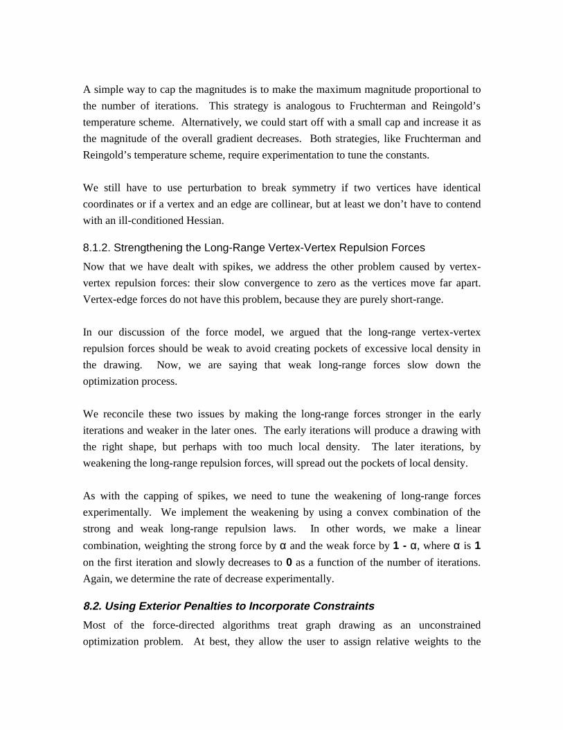
A simple way to cap the magnitudes is to make the maximum magnitude proportional to
the number of iterations. This strategy is analogous to Fruchterman and Reingold’s
temperature scheme. Alternatively, we could start off with a small cap and increase it as
the magnitude of the overall gradient decreases. Both strategies, like Fruchterman and
Reingold’s temperature scheme, require experimentation to tune the constants.
We still have to use perturbation to break symmetry if two vertices have identical
coordinates or if a vertex and an edge are collinear, but at least we don’t have to contend
with an ill-conditioned Hessian.
8.1.2. Strengthening the Long-Range Vertex-Vertex Repulsion Forces
Now that we have dealt with spikes, we address the other problem caused by vertex-
vertex repulsion forces: their slow convergence to zero as the vertices move far apart.
Vertex-edge forces do not have this problem, because they are purely short-range.
In our discussion of the force model, we argued that the long-range vertex-vertex
repulsion forces should be weak to avoid creating pockets of excessive local density in
the drawing. Now, we are saying that weak long-range forces slow down the
optimization process.
We reconcile these two issues by making the long-range forces stronger in the early
iterations and weaker in the later ones. The early iterations will produce a drawing with
the right shape, but perhaps with too much local density. The later iterations, by
weakening the long-range repulsion forces, will spread out the pockets of local density.
As with the capping of spikes, we need to tune the weakening of long-range forces
experimentally. We implement the weakening by using a convex combination of the
strong and weak long-range repulsion laws. In other words, we make a linear
combination, weighting the strong force by α and the weak force by 1 - α, where α is 1
on the first iteration and slowly decreases to 0 as a function of the number of iterations.
Again, we determine the rate of decrease experimentally.
8.2. Using Exterior Penalties to Incorporate Constraints
Most of the force-directed algorithms treat graph drawing as an unconstrained
optimization problem. At best, they allow the user to assign relative weights to the

different forces. Little work has addressed the problem of general graph drawing with
constraints. A few approaches allow the user to fix the positions of particular vertices.
The most relevant work, that of He and Mariott [HM96] , allows only linear equalities and
inequalties as constraints.
The possibility of specifying constraints makes a graph drawing algorithm more flexible.
A user might introduce constraints to anchor certain vertices at fixed positions or to
restrict them to particular regions of the drawing space. Constraints can also control the
positions of vertices relative to one other, thus portraying clusters of vertices or particular
relationships among the constrained vertices.
We incorporate constraints into our model by using the method of exterior penalties.
This method requires, for each constraint, an efficient procedure to measure the distance
(in R2n) from an infeasible drawing to the nearest drawing that satisfies the constraint.
We use these procedures to add penalty terms to the objective function that increase over
time, so that eventually all descent directions will point towards the feasible space.
Several caveats are in order.
First, the method of exterior penalties is not applicable to infeasible problems—that is,
problems for which no solution satisfies all of the constraints. These problems are better
addressed by a two-phase approach that first chooses a subset of constraints to be
satisfied and then solves the resulting constrained optimization problem.
Second, the method can break down when the feasible space is disconnected. A one-
dimensional example illustrates this possibility. Let us imagine that we have a single
variable x, a trivial objective function that is always equal to 1, and two constraints. The
first constraint is that x ∈ [1, 2] ∪ [3, 4] ; the second is that x ∈ [-2, -1] ∪ [3, 4] . Let us
imagine that we start with the infeasible point x = 0. The penalty term for the first
constraint will point us in the positive direction, towards the nearest point that satisfies
the constraint, x = 1. The penalty term for the second constraint, however, will point us
towards x = -1. Because these two terms will cancel out, we will never find the feasible
space, which is x ∈ [3, 4] .
Third, the magnitudes of the penalty terms should not be too large relative to the
magnitude of the gradient. They should be just large enough to force the optimization

procedure towards the feasible space. If we make the penalties too large, then they will
create the problems of spikes that we discussed earlier. Often, we do not have to make
the penalties very large for the optimization procedure to discover the feasible space.
We have had good results with quadratic penalty terms. For each constraint, we make the
corresponding penalty term the square of the vector difference between the current
drawing and the closest drawing that satisfies the constraint. We call the negative
gradient of the sum of all such penalties the penalty vector, and we add a multiple of this
penalty vector to the negative gradient that we compute from the force laws.
Let us denote the penalty vector by p and the negative gradient by -g. Let θ be the angle
between p and -g, i.e. cos θ = p • (-g) / ||p|| ||-g||. Then, if cos θ is positive, ignoring
p and following the negative gradient will bring us closer to the feasible space, while, if
cos θ is negative, doing so will take us away from the feasible space. The more negative
the cosine, the greater we need to make our coefficient for p.
In our implementation, this coefficient is max(ε, ε - cos θ) * max(1, (||- g|| / ||p||)),
where ε = 10-8. The first factor uses the cosine to weight the penalty vector, while the
second factor normalizes the negative gradient and penalty vectors. This formula is
surely not optimal, but it works well in practice and is simple to compute.
We refer the reader to Gill, Murray, and Wright [GMW81] for further discussion of the
method of exterior penalties and related numerical optimization methods.
8.3. Introducing Additional Degrees of Freedom
Our last application of scheduling is to take an unconstrained graph drawing problem and
turn it into a constrained problem in a larger drawing space, which we solve using
exterior penalties. We transform the problem in order to take advantage of the
maneuvering room in the larger space.
Before describing this technique, let us consider an example of what happens when the
drawing space has only one dimension rather than two. We take a simple undirected
graph: three vertices v1, v2, v3 and two edges e1 = (v1, v2), e2 = (v2, v3).
The drawing on the left in Figure 8.1 shows the globally optimal drawing. Unfortunately,
a local optimization procedure will only converge to this optimum (or its mirror image) if

v2 is between v1 and v3 in the initial drawing. If the initial placement is random, this
happy event occurs with probability 1/3. With probability 2/3, a local optimization
procedure will converge to the drawing on the right (or one of the three other equivalent
drawings), which is locally optimal but lousy.
v2 v3v1 v3 v2v1
Figure 8.1: Local optima for a 3-vertex graph in one dimension.The drawing on the left is globally optimal.
While one-dimensional graph drawing may seem a contrived problem, it arises in code
and data layout applications [Be94]. In any case, using local optimization methods in one
dimension is clearly a poor strategy. A much better approach is to move the problem to a
two-dimensional space and then somehow squash it back onto one dimension. In two
dimensions, the graph above would, with probability 1, be drawn as some rotation of the
global optimum.
How do we squash the problem back onto its original drawing space? In this example,
we can introduce the constraint yi = 0 for each vertex vi. We then apply the method of
exterior penalties to solve the constrained problem.
We can use this same strategy to convert an unconstrained two-dimensional problem into
a constrained three-dimensional problem. Here, the constraint is zi = 0 for each vertex vi,
and the corresponding penalty terms are zi2. By lifting the problem from two dimensions
to three or more dimensions, we can often “untwist” drawings that would otherwise
converge to poor local minima.

9. Vertex Size and Shape
Thus far, we have used a force model in which vertices are represented by dimensionless
points. While doing so has simplified our discussion thus far, we must take vertex size
and shape into consideration in order to make our graph drawing algorithm relevant to
practical problems.
In this chapter, we adapt the force laws to take into account vertex shape and size. We
require that the vertex shapes are convex; if they are not, we can satisfy this requirement
by replacing a vertex shape with its convex hull. We also require, for the sake of
efficiency, access to a constant-time test that determines if and where a single line
segment intersects the boundary of a given vertex. Such a test is straightforward when
the vertices are drawn as rectangles, as is most commonly the case.
Vertex size and shape affect our force laws for edge springs, vertex-vertex repulsion, and
vertex-edge repulsion. When vertices are large, we need to modify our force laws to
make room for them. The modifications should be primarily short-range, since the size
and shape of a vertex rapidly decrease in importance as we move away from it.
9.1. Vertex Radii
It is convenient to always measure the distance between two vertices by using the line
segment connecting the vertex centers. We have to consider, however, that the distance
between the vertex boundaries depends on the size and shape of the vertices, as well as
the orientation of the line segment. In particular, we have to subtract out the “radius” of
each vertex—that is, the distance from the center of each vertex to the point at which the
line segment intersects the vertex boundary. We refer to these distances as the radii of
the vertices with respect to the line segment connecting them. When there is no
ambiguity, we simply refer to them as the vertex radii.
Figure 9.1 shows how we measure the radii of vertices v1 and v2 when we are computing
the distance between them. We first draw the line segment connecting the vertex centers,
and then we compute the distances between the centers and the intersections of this line
segment with the vertex boundaries to obtain the vertex radii r1 and r2.

v1
v2
r 1
r 2
Figure 9.1: The radii of rectangular vertices v 1 and v 2
with respect to the line segment connecting them.
9.2. Adapting the Force Laws to Consider Vertex Radii
In order to take vertex radius into account, we make several changes to the force laws.
First, we give the edge springs a non-zero rest length that reflects the radii of the
endpoints with respect to the edge. Then, we modify the vertex-vertex repulsion law in
order to make the boundary-to-boundary rest length of an edge equal to k. Finally, we
make a similar modification to the vertex-edge repulsion force.
9.2.1. Increasing the Rest Length of Edge Springs
In the force model we have described thus far, the springs have a rest length of zero—that
is, they always try to pull their endpoints closer together. While this works well for
dimensionless vertices, it does not make as much sense when vertices have nontrivial size
and shape.
In order to reflect vertex size and shape, we make the rest length of an edge spring equal
to the sum of the endpoint radii. Accordingly, the spring pushes the endpoints away from
each other when the endpoints overlap, since the distance between the centers is less than
the sum of the radii. When the endpoints are mutually tangent, the spring exerts no force
on them. Finally, if the endpoints are further apart than the sum of their radii, then the
spring pulls them towards each other.
For an edge connecting dimensionless vertices vi and vj , our formula for the magnitude
of the spring force was ||fspring (vi, vj)|| = ||xi - xj||2 / k.

If the radii of v1 and v2 with respect to the line segment connecting them are r1 and r2,
then we make the magnitude ||fspring (vi, vj)|| = (||xi - xj|| - (r1 + r2))2 / (k + (r 1 + r2)).
The direction of the spring force (pulling the vertices towards or pushing them away from
each other) depends on whether dist(v i, vj) is greater than or less than r1 + r2. A
reminder: we measure ||xi - xj|| as the length of the line segment connecting the vertex
centers.
9.2.2. Modifying the Vertex-Vertex Repulsion Law
We had set up our edge spring and vertex-vertex repulsion laws so that an edge would
have a rest length of k. Now that we have modified the spring law to consider the vertex
radii, we need to make a corresponding change to the vertex-vertex repulsion law.
For dimensionless vertices, we had the following formula for the magnitude of the
repulsion force: ||frepulsion (vi, vj)|| = k2 / ||xi - xj||.
If the radii of v1 and v2 with respect to the line segment connecting them are r1 and r2,
then we replace this formula with ||frepulsion (vi, vj)|| = (k + (r 1 + r2))2 / ||xi - xj||.
As we discussed earlier, using a single law for vertex-vertex repulsion can cause
excessive local density. If we distinguish between strong short-range and long-range
repulsion, then the above law is for short-range repulsion, and the modification to the
inverse-square long-range repulsion law is analogous.
9.2.3. Modifying the Vertex-Vertex Repulsion Law
Finally, we need to modify the vertex-edge repulsion law to reflect the vertex size and
shape.
In our model for dimensionless vertices, we made the magnitude of the vertex-edge
repulsion force ||frepulsion (vi, ej)|| = cve((k2 / x) - k) when x, the distance between
vertex vi and edge ej, is less than k.
Applying the same idea we used for vertex-vertex repulsion, we replace k by k + r , where
r is the radius of vi with respect to the shortest line segment connecting it to ej.
Accordingly, the new magnitude is ||frepulsion (vi, ej)|| = cve(((k+r)2 / x) - (k+r)) when x,
the distance between the center of vertex vi and edge ej, is less than k + r .

9.3. Adapting the Procedure to Compute the Forces
Since we are modifying the force laws to take vertex size and shape into account, we also
have to make changes to the procedure for computing the forces. In particular, we have
to modify the Barnes-Hut algorithm that we use for computing vertex-vertex repulsion
and the distance cut-off procedure that we use for computing vertex-edge repulsion. We
will assume for simplicity that all vertices are rectangles, but our methods apply as long
as the vertices conform to simple, parameterized class of shapes, such as ellipses.
The change we make to the Barnes-Hut procedure is that we store in each cell the average
shape of a vertex. Since our vertices are rectangles, we simply maintain the average
width and height of the vertices in each cell. Then, when we approximate the repulsion
that the cell exerts with its centroid, we use this width and height in our computation.
For our computation of vertex-edge repulsion, we have to modify the assignment of
vertices to grid cells to take radius into account. We store each vertex in every grid cell
that it intersects. Then, when we iterate for each edge through the grid cells it occupies
(including all of the grid cells occupied by the endpoints) and the neighbors of those cells,
we will find all vertices within the short range of the edge.

10. Qualitative Results: A Gallery of Examples
Until now, we have focused on the details of our algorithm. Now, we look at the
performance of an implementation that we have written in Java. In this chapter, we take a
qualitative perspective: we present a variety of drawing produced by our implementation
and discuss the strengths and weakness of the algorithm on different classes of graphs in
intuitive terms. In Chapter 11, we will take a more quantitative perspective.
Our presentation of drawings is in order of increasing density. We start from trees, the
sparsest of graphs, and work our way up to complete graphs. We only consider graphs
that are connected, since it is not difficult to find the connected components of a graph
and draw them separately.
10.1. Trees
Trees are the sparsest of connected graphs: a tree of n vertices has m = n − 1 edges.
Tree drawing is a well studied problem, and there are good, special-purpose algorithms
for drawing both rooted (directed) and unrooted trees [RT81, Ea92].
It is surprising, perhaps, that force-directed algorithms perform very badly on trees. In
fact, trees are some of the worst inputs for graph drawing algorithms based on numerical
optimization. Trees have two qualities that confound force-directed algorithms. The first
is that they have countless poor local minima that result from swapping the positions of
subgraphs so that they cross. The second is that, because trees are so sparse, the spring
forces do not particularly restrict the movement of vertices; instead, it is the repulsion
forces that largely determine the placement of vertices. Because the repulsion forces are
far less smooth than the spring forces, they slow down any first-order numerical
optimization, such as steepest descent of the conjugate gradient method.
Nonetheless, we have two reasons to test our algorithm on trees. The first is
completeness: since our algorithm applies to all connected graphs, it behooves us to test it
on as wide a range of input graphs as possible. The other reason is that we can compare
the performance of our algorithm with that of other force-directed approaches, and
thereby see the relative strengths and weakness of our techniques.

The drawings that our algorithm produces are similar to those produced by radial tree
drawing algorithms, only that ours tend to distribute vertices more evenly throughout the
drawing area. Unlike the radial drawing algorithms, however, we do not always produce
crossing-free drawings of trees. In general, drawings of trees that have edge crossings
correspond to poor local minima.
We did experiment with modifying the force laws to produce more traditional drawings
of rooted trees (see the discussion of “eumorphous” drawings in Section 3.1.1), where all
edges were directed towards the root and pointed upwards. Unfortunately, we found that
the aesthetic principles for eumorphous drawings of trees were very different from those
for general graphs. While our force-directed drawings aim to distribute vertices
uniformly throughout the drawing space, traditional drawings of rooted trees tend to be
much denser at the bottom, where the leaves are, than at the top, where the root is, and
they are generally much wider that they are tall.
Let us consider, for example, a complete binary tree of n = 2h-1 vertices. Our force-
directed algorithm will produce a drawing that roughly occupies a square drawing area
whose side is k n . In contrast, a eumorphous drawing will have h layers and 2h-1
leaves—roughly half of the vertices—occupying the lowest of the layers. In order for the
height and width of the drawing area to be equal, the vertical separation between layers
would have to be 2h-1 / h (roughly n / log n ) times larger than the horizontal separation
between vertices on the lowest layer.
We experimented with various schemes involving constraints and modifications of the
spring laws for directed edges, but none of them consistently produced satisfactory
drawings of rooted trees.
Given the difficulty that force-directed algorithms have drawing trees, we suspect that a
general graph drawing algorithm should use a hybrid approach. First, it should compute
the unique tree of biconnected components—that is, the maximal subgraphs that cannot
be disconnected by the removal of a vertex. It should then use a specialized tree-drawing
algorithm to arrange the centroids of these biconnected components. Finally, it should
draw each component independently using a force-directed algorithm—with the centroids
fixed according to the previous step. We discuss such an approach, as well as its pitfalls,
in the section on future work.

We now present a few examples of trees produced by our algorithm.
Figure 10.1 shows a complete binary tree of 63 vertices. To produce this drawing, we
used a three-dimensional drawing space with two-dimensional constraints, as described in
section 8.3. Figure 10.2 shows an example of the many poor local minima that often
result when we apply our algorithm directly on a two-dimensional drawing area.
Figure 10.1: Complete Binary Tree of 63 Vertices
Figure 10.2: Example of Bad Local Minimum

Figure 10.3 shows a random tree of 100 vertices; here we can see clearly that the drawing
is not radial, but rather that the vertices spread themselves out relatively uniformly
throughout the drawing area.
Figure 10.3: Random Tree of 100 Vertices
10.2. Planar Biconnected Graphs
As we have discussed, the performance of force-directed algorithms suffers for trees, and
in general for graphs that are not biconnected. We therefore turn our attention to
biconnected graphs. We start with an important class of biconnected graphs: graphs that
are biconnected and planar.
Planar graphs are of particular theoretical and practical interest. Planar graphs, by
definition, can be drawn in the plane without any edge crossings. Many classical results
in graph theory pertain to planar graphs: Fary determined that a planar graph could be
drawn without edge crossings using straight-line edges [Fa48]; Hopcroft and Tarjan
determined how to both test the planarity of a graph and compute an embedding of it in
linear time [HT74] ; Tutte proposed a “barycenter” method for drawing planar graphs that
was suggestive of the later force-directed approaches and that would always converge to a
drawing without edge crossings [Tu60]. The practical significance of planar graphs
comes from their ubiquity: maps are the face-duals of planar graphs; circuits laid out on a
board cannot have edge crossings; roads and railroad tracks cannot arbitrarily cross each
other; and so forth.

A classic result of Euler is that a planar graph of n vertices has at most m ≤ 3n − 6 edges
[BM76] . Planar graphs are therefore quite sparse: the average degree of a vertex is at
most six.
In general, sparse graphs are harder for force-directed algorithms to draw than dense ones
because the repulsion forces are not as smooth as the spring forces. Nonetheless,
biconnected planar graphs are generally easier to draw than trees. The sparsest of
biconnected planar graphs are cycles, where every vertex has a degree of two. Cycles,
like trees, are susceptible to poor local minima because of their sparseness; these local
minima generally result from the cycles getting tangled. At the other extreme, we have
triangular meshes, where the average degree is almost six. These graphs, not surprisingly,
are much easier for force-directed algorithms to draw.
Regardless of the planarity of the graph, our algorithm does not attempt to avoid edge
crossings. Similarly, our algorithm does not treat graphs of three-dimensional objects in
any special way—that is, the algorithm does not take into account the fact that their
topologies correspond to those of three-dimensional objects.
Figure 10.4 shows a drawing of a cycle of 100 vertices. In general, cycles are optimally
drawn as regular polygons. Interestingly, they are drawn as such even when placed in a
higher dimensional space—that is, they will occupy a planar slice of that space.
Figure 10.4: Cycle of 100 Vertices

Force-directed algorithms work especially well for planar meshed. Figure 10.5 shows a
triangular mesh of 465 vertices. Figure 10.6 shows a square mesh of 400 vertices. As
with trees, using a third dimension allows the drawing to untwist itself out of tangles.
Like cycles, planar meshes will be drawn as planar even when placed in a higher
dimensional space.
Figure 10.5: Triangular Mesh of 465 Vertices
Figure 10.6: Square Mesh of 400 Vertices
Figure 10.7 shows two drawings of a graph corresponding to the topology of a
dodecahedron. Interestingly, both graphs drawings were produced in two dimensions.
Neither is crossing-free, since a crossing-free drawing would require a high variance in
edge length. The drawing on the left appears to be three-dimensional.
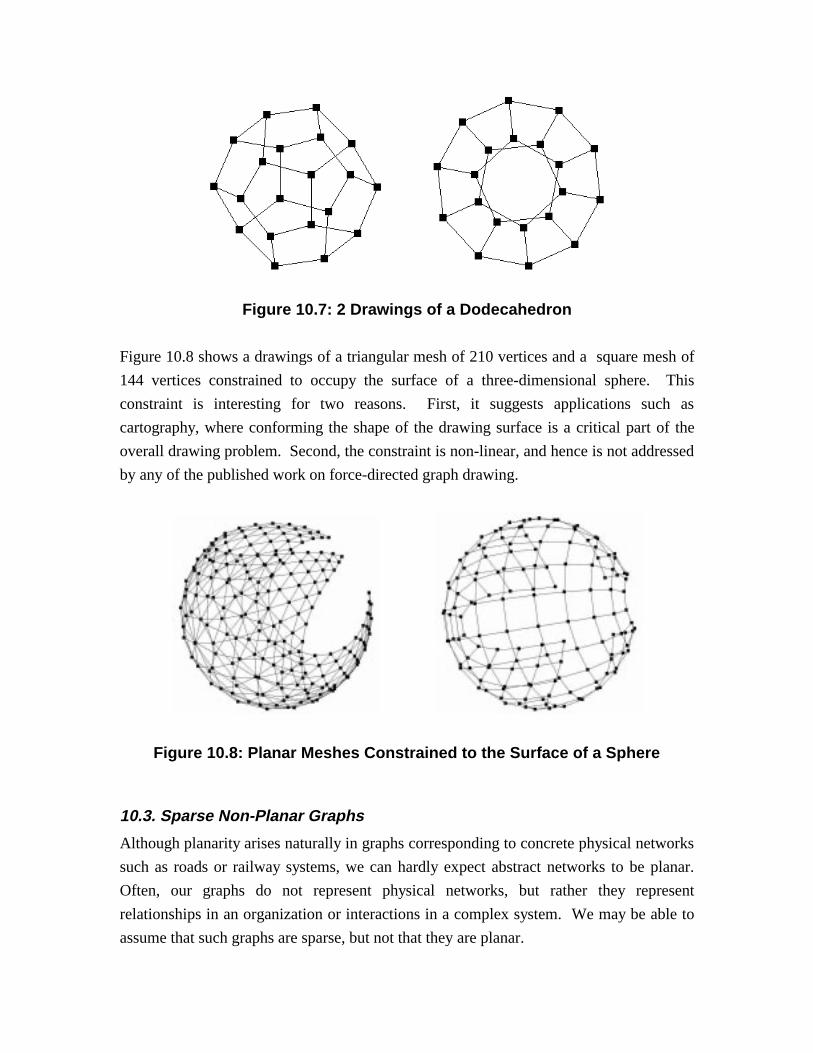
Figure 10.7: 2 Drawings of a Dodecahedron
Figure 10.8 shows a drawings of a triangular mesh of 210 vertices and a square mesh of
144 vertices constrained to occupy the surface of a three-dimensional sphere. This
constraint is interesting for two reasons. First, it suggests applications such as
cartography, where conforming the shape of the drawing surface is a critical part of the
overall drawing problem. Second, the constraint is non-linear, and hence is not addressed
by any of the published work on force-directed graph drawing.
Figure 10.8: Planar Meshes Constrained to the Surface of a Sphere
10.3. Sparse Non-Planar Graphs
Although planarity arises naturally in graphs corresponding to concrete physical networks
such as roads or railway systems, we can hardly expect abstract networks to be planar.
Often, our graphs do not represent physical networks, but rather they represent
relationships in an organization or interactions in a complex system. We may be able to
assume that such graphs are sparse, but not that they are planar.

Our algorithm does not take edge crossings into account; rather, its performance depends
mostly on the sparseness or density of the input graph. Of course, given a non-planar
input graph, it will always produce a drawing that has edge crossings. In general, the
denser the graph, the easier and faster it is for the numerical optimization procedure to
converge to a local minimum. On the other hand, denser graphs often result in less
legible drawings than sparser ones, because the edges clutter the drawing.
We have chosen examples for this section from two families of non-planar graphs where
m is θ(n).
A cycle of n/c c-cliques (i.e. copies of Kc) is non-planar if c ≥ 5 and has an average
degree of roughly c-1. Figure 10.9 shows a cycle of 20 Kcs.
Figure 10.9: Cycle of 20 K 5s
A torus is a non-planar graph constructed by taking a square mesh and connecting the top
to the bottom and the left to the right. Every vertex in a torus has degree four. Figure
10.10 shows a torus of 256 drawn in both two and three dimensions. The drawing on the
left misleadingly appears to be three-dimensional, but the drawing on the right, which is
in fact three-dimensional, best reveals the structure of the graph.

Figure 10.10: Torus of 256 Vertices in Two and Three Dimensions
10.4. Dense Graphs
Finally, we consider denser graphs where m is not θ(n). If m is θ(n log n) , then the
time necessary to compute the spring forces will be within a constant factor of the time
necessary to compute the vertex-vertex repulsion forces using the Barnes-Hut procedure.
If m is θ(n2), we have no reason to use the Barnes-Hut procedure: since we will require
θ(n2) time to compute the gradient, we may as well compute the repulsion forces exactly.
In fact, we might even use Kamada and Kawai’s algorithm, since we will already need
θ(n2) space to store the graph.
While increasing the density of a graph beyond an average degree of θ(log n) increases
the time necessary to compute the gradient, it does decrease the number of iterations
necessary for convergence, since the spring forces are smoother than the repulsion forces,
and the spring forces dominate the repulsion forces in dense graphs.
Most drawings of dense graphs are too cluttered with edges to be useful. Some
exceptions are hypercubes, complete bipartite graphs, and complete graphs, like those we
show below. We doubt that many practical applications require drawings of dense
graphs, but we include this section for completeness.

A d-dimensional hypercube has 2d vertices, each of degree d. Figure 10.11 shows
drawings of a 6-dimensional hypercube of 64 vertices in drawing spaces of two and three
dimensions.
Figure 10.11: 6-Dimensional Hypercube in Two and Three Dimensions
The complete bipartite graph Kn1,n2 has n1+n2 vertices and n1n2/2 edges. Figure 10.12
shows two two-dimensional drawings of K6,6. In the drawing on the right, the vertices
have been constrained to lie on a circle.
Figure 10.12: The Complete Bipartite Graph K 6,6

Finally, the complete graph Kn has n vertices, each of degree n-1. Figure 10.13 shows a
two-dimensional drawing of K30. We have made the vertices a bit larger so that they are
clearer against the clutter of the 435 edges.
Figure 10.13: The Complete Graph K 30

11. Quantitative Results
While the previous chapter illustrates output generated by our algorithm, the drawings are
fairly typical of those produced by all force-directed algorithms. Given that our main
contribution is to improve the performance of such algorithms, we now shift to a more
quantitative perspective to demonstrate this improvement.
We do so in three ways. First, we analyze our approach and compare it to others in terms
of its computational complexity. Unfortunately, this analysis does not help us understand
the number of iterations required to converge to a locally optimal drawing. We therefore
perform experiments to see how the number of iterations required for convergence
depends on both the size and density of the graph. Finally, we look at the time required to
compute each of these drawings, and compare our times to those presented in other
papers on force-directed algorithms.
We obtained all of our results with a Java implementation of our algorithm running on a
Pentium 133 MHz machine under the Microsoft Windows 95 operating system. We
used Sun Microsystems’s JDK version 1.1.7 as our Java compiler and interpreter.
11.1. Computational Complexity
The computational complexity of an iteration, as shown in Chapter 6, is θ(m + n log n) .
Briefly reviewing, we take θ(m) time to compute the spring forces, θ(n log n) time to
compute the vertex-vertex repulsion forces using the Barnes-Hut algorithm, and θ(m)
time to compute the vertex-edge repulsion forces using distance cut-offs.
This computational complexity compares very favorably to those of other algorithms in
the literature, as shown by the table in Figure 11.1. We note that, for the algorithms of
Kamada and Kawai [KK89] , Davidson and Harel [DH96], and Tunkelang [Tu94], we
report the complexity of n iterations, since, for these three algorithms, each iteration only
moves a single vertex as compared to moving all n vertices in all of the other algorithms.
We also recall that Kamada and Kawai’s algorithm uses a preprocessing phase that
requires θ(n2) space and θ(n3) time. Finally, we note that some of the running times
depend on the distribution of vertices being sufficiently uniform—namely, the
computation of vertex-vertex repulsion forces in Fruchterman and Reingold’s “grid
variant” and computation of vertex-edge repulsion in our own algorithm.

SpringsVertex-Vertex
Repulsion
Vertex-Edge
RepulsionCrossings TOTAL
[Ea84] θ(m) θ(n2) θ(n2)
[FR91] θ(m)θ(n2)
θ(n) for grid variant
θ(n2)
θ(m)
[FLM94] θ(m) θ(n2) θ(n2)
[Tu94] θ(m)θ(n2)
θ(n) for grid variant
θ(nm)
θ(m)
θ(m2)
θ(m)
θ(m2)
θ(m)
[KK89] θ(n2) θ(n2)
[DH96] θ(m) θ(n2) θ(nm) θ(m2) θ(m2)
proposed
algorithmθ(m) θ(n log n) θ(m)
θ(m +
n log n)
Figure 11.1: Computational Complexity of Computing the Negative Gradient
As we can see in the table, the computation of vertex-vertex repulsion forces is generally
the bottleneck. The Barnes-Hut algorithm allows us to reduce the complexity of this step
from θ(n2) to θ(n log n) without incurring the extreme loss of accuracy of the “grid
variant” method (i.e. distance cut-offs). Unlike several of the algorithms, ours does take
vertex-edge repulsion into account; unfortunately, including edge-crossings would not
only be expensive, but would also rule out our optimization approach.
11.2. Number of Iterations
We have seen that the running time of our algorithm on a single iteration is
asymptotically better than those of the published force-directed algorithms. We now look
at the number of iterations required for convergence.
Unfortunately, all of the papers in the literature are evasive on this point. Most use a
fixed number of iterations; Kamada and Kawai are the exception in that their termination
condition depends on the maximum energy among the vertices. The authors that
comment on the number of iterations generally speculate that it is proportional to the
number of vertices. Unfortunately, there is no systematic study of the performance of
graph drawing algorithms on large graphs, perhaps because the θ(n2) inner loop of the
published algorithms makes such a study prohibitive.

In order to gain some insight into the number of iterations required for convergence, we
ran a suite of experiments. We used several families of graphs: paths, cycles, complete
binary trees, square meshes, hypercubes, and complete graphs. For each family, we
selected a set of graphs of varying sizes, in order to measure the number of iterations as a
function of the size. In order to test the relative performance of steepest descent and the
conjugate gradient method, we tested all of our graphs with both optimization procedures.
For each graph and optimization procedure, we ran our algorithm ten times on random
initial drawings, and then computed the mean number of iterations required for
convergence. We used a straightforward, if conservative, convergence criterion: the
algorithm terminates when an iteration moves no vertex more than half of a pixel. Since
our line search is reasonably accurate, this criterion all but guarantees that the final
drawing is visually indistinguishable from a local optimum.
The plots that follow confirm two observations that we have made in earlier chapters.
First, the conjugate gradient method consistently outperforms steepest descent, and the
gap widens as n increases. Second, the number of iterations required for convergence
decreases as the density increases. We note that a conjugate gradient iteration is only
slightly more expensive than that for a steepest descent iteration; in particular, computing
the descent direction requires only one gradient computation in either case.
Figure 11.2: Performance on Paths
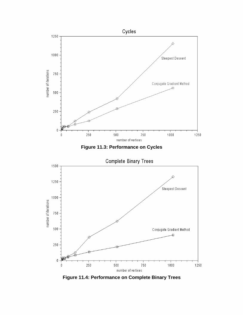
Figure 11.3: Performance on Cycles
Figure 11.4: Performance on Complete Binary Trees

Figure 11.5: Performance on Square Meshes
Figure 11.6: Performance on Hypercubes

Figure 11.7: Performance on Complete Graphs
11.3. Running Time
A review of the literature reveals that very few papers even consider the performance of
force-directed algorithms on large graphs. In fact, we could only find one paper that
reported running times for graphs of over a hundred vertices.
Frick et al., report running times of 9.19 seconds for a complete binary tree of 127
vertices, 9.54 seconds for a path of 128 vertices, 45.04 seconds for a binary tree of 255
vertices, 37.93 seconds for a path of 256 vertices, and 71.78 seconds for a square mesh of
256 vertices. They estimate that the number of iterations is linear in the number of
vertices, and hence that their running time is θ(n3), which would imply that doubling the
number of vertices would multiply the running time by eight.
Not only do we achieve better running times, but our algorithm scales more gracefully
because of both the Barnes-Hut and conjugate gradient procedures. If we make the same
assumption as Frick et al. that the number of iterations is linear in the number of vertices,
then our running time is θ(n2 log n) , which would imply that doubling the number of
vertices roughly multiplies the running time by four. If, as convergence analysis of the

conjugate gradient method suggests, the number of iterations is proportional to the square
root of the number of vertices, then this difference is even larger.
The plot below shows the running times for the families of graphs we have described in
the previous section. As we can see, for graphs of the same number of vertices, the
running time decreases as the density increases. Unfortunately, our implementation could
not handle large complete graphs.
Figure 11.8: Running Times on a Variety of Input Graphs

12. Conclusions and Future Work
The principle contribution of this dissertation is to approach graph drawing using time-
tested techniques from other fields. The original impetus for this work was an insight
about replacing the fixed step size in published force-directed algorithms with a primitive
line search procedure. Indeed, the adaptive line search procedure that we use is a major
improvement on either using a fixed step size or complicating the algorithm with a
“temperature” scheme. In general terms, however, we furthered the state of the art by not
treating graph drawing as an isolated field.
From numerical optimization, we learned that we could achieve a better rate of
convergence with conjugate gradients than with steepest descent. We also learned to pay
better attention to the smoothness of the objective function. Finally, we were able to take
advantage of the method of exterior penalties, both to incorporate a general class of
constraints into our model and to avoid poor local minima.
From the many-body simulation literature, we borrowed the Barnes-Hut algorithm. This
improvement is perhaps the most critical to making graph drawing scale to large graphs.
Finally, we had some new insights specific to graph drawing. In particular, our handling
of vertex shape and size and our introducing a vertex-edge repulsion force make the
general graph drawing model much more relevant to real visualization problems.
Of course, there are many open problems in graph drawing. Here are some questions that
suggest directions for future work:
1) Can we make a rigorous theoretical analysis of the number of iterations required
for convergence?
Both the method of steepest descent and the conjugate gradient method lend themselves
to theoretical analysis. Indeed, the former can be shown to have a linear rate of
convergence, while the latter can be show to have a superlinear rate. A more accurate
analysis of the rate of convergence requires that we know the condition number of the
Hessian of the objective function we are minimizing. Since our objective function is not
quadratic, the Hessian is not a constant, and therefore the condition number changes from

iteration to iteration. A deeper understanding of the convergence properties of different
optimization procedures on graph drawing problems probably requires analytical
techniques that specifically address this varying condition number.
2) Can we incorporate discrete terms, such as edge crossings, into a model based on
continuous optimization?
There is a consensus in the graph drawing community that, all else equal, it is best to
avoid edge crossings. Unfortunately, all else is not equal. The main problem with
incorporating edge crossings into a continuous optimization approach is that the number
of edge crossings is a discrete term. What would be ideal is a continuous term that
correlates, at least approximately, to the number of edge crossings.
3) Can we design an algorithm that recognizes easy patterns in a graph and uses a
divide-and-conquer approach to draw the graph more efficiently?
A first step in this direction would be to split a graph into its biconnected components, as
we discussed in Section 10.1. To review, the idea is to lay out the centroids of the
biconnected components using a specialized tree-drawing algorithm, and then to apply
our force-directed algorithm to each biconnected component separately, fixing its
centroid to where the tree-drawing algorithm placed it.
This approach, however, needs to address the subtlety that the edges connecting vertices
in different biconnected components will be affected by the placement of their endpoints
within their respective components. Moreover, it only helps us when we have a
significant number of biconnected components. It would be nice to explore more
sophisticated heuristics, such as partitioning the graph using small separators.
4) Can we do better than local optimization, e.g. can we obtain a drawing whose
energy is within some constant multiple of the globally optimal energy?
This problem, as far as we know, has been completely open since Eades wrote his first
paper on the spring model. An approach with guaranteed bounds in terms of the globally
optimal energy would seem to require a much deeper understanding of the problem than
we have thus far. We have nothing to offer but encouragement.
5) Can we achieve drawings that conform to the aesthetics of the force-directed
model without resorting to continuous optimization?
The only techniques in the graph drawing literature that address general graphs are the
topology-shape-metrics model and the force-directed model. The former only applies to
orthogonal graph drawing problems. The latter, while useful, is fraught with problems,
ranging from vulnerability to poor local minima to performance issues. Is there an
alternative technique for producing drawings with the aesthetics that the force-directed
model aims to quantify?

Bibliography
[Be94] B. Beckman, “Theory of Spectral Graph Layout,” Technical Report MSR-TR-94-
04, Microsoft Research, 1994.
[BH86] J. Barnes and P. Hut, “A Hierarchical O(N log N) Force-Calculation Algorithm,”
Nature, vol. 324, pp. 446-449, 1986.
[BK94] T. Biedl and G. Kant, “A Better Heuristic for Orthogonal Graph Drawings,” in
Proceedings of the Second Annual European Symposium on Algorithms, vol. 855
of Lecture Notes in Computer Science, pp. 24-35, 1994.
[BM76] J. Bondy and U. Murty, Graph Theory with Applications, Macmillan, London,
1976.
[Ca80] M. Carpano, “Automatic Display of Hierarchized Graphs for Computer-Aided
Decision Analysis,” IEEE Transactions on Systems, Man, and Cybernetics, vol.
10, no. 11, pp. 705-715, 1980.
[CLR90] T. Cormen, C. Leiserson, and R. Rivest, Introduction to Algorithms, MIT
Press, London, 1990.
[CP96] M. Coleman and D. Parker, “Aesthetics-based Graph Layout for Human
Consumption,” Software—Practice and Experience, vol. 26, no. 12, pp. 1415-
1438, 1996.
[DETT94] G. Di Battista, P. Eades, R. Tamassia, and I. Tollis, “Algorithms for Drawing
Graphs: An Annotated Bibliography,” Computational Geometry, vol. 4, pp. 235-
282, 1994.
[DETT99] G. Di Battista, P. Eades, R. Tamassia, and I. Tollis, Graph Drawing, Prentice-
Hall, New Jersey, 1999.
[DH96] R. Davidson and D. Harel, “Drawing Graphs Nicely Using Simulated
Annealing,” ACM Transactions on Graphics, vol. 15, no. 4, pp. 301-331, 1996.

[Ea84] P. Eades, “A Heuristic for Graph Drawing,” Congressus Numerantium, vol. 42,
pp. 149-160, 1984.
[Ea92] P. Eades, “Drawing Free Trees,” Bulletin of the Institute for Combinatorics and
its Applications, vol. 5, pp. 10-36, 1992
[ES90] P. Eades and K. Sugiyama, “How to Draw a Directed Graph,” Journal of
Information Processing, vol. 13, no. 4, pp. 424-437, 1990.
[Fa48] I. Fary, “On Straight Lines Representations of Planar Graphs,” Acta Scientiarum
Mathematicarum, vol. 11, pp. 229-233, 1948.
[FCW67] C. Fisk, D. Caskey, and L. West, “ACCEL: Automated Circuit Card Etching
Layout,” in Proceedings of the IEEE, vol. 55, no. 11, pp. 1971-1982, 1967.
[FLM94] A. Frick, A. Ludwig, and H. Mehldau, “A Fast Adaptive Layout Algorithm for
Undirected Graphs,” in [GD94], pp. 388-403.
[FR91] T. Fruchterman and E. Reingold, “Graph Drawing by Force-Directed Placement,”
Software—Practice and Experience, vol. 21, no. 11, pp. 1129-1164, 1991.
[GD93] G. Di Battista, H. de Frayssseix, P. Eades, P. Rosenstiehl, and R. Tamassia, eds.,
Proceedings of ALCOM International Workshop on Graph Drawing and
Topological Graph Algorithms (Graph Drawing ’93), Paris, France, 1993.
[GD94] R. Tamassia and I. G. Tollis, eds., Proceedings of DIMACS International
Workshop, GD ‘94, Princeton, New Jersey, USA, vol. 894 of Lecture Notes in
Computer Science, 1994.
[GD95] F. J. Brandenburg, ed., Proceedings of Symposium on Graph Drawing, GD ‘95,
Passau, Germany, vol. 1027 of Lecture Notes in Computer Science, 1995.
[GD96] S. North, ed., Proceedings of Symposium on Graph Drawing, GD ‘96, Berkeley,
California, USA, vol. 1190 of Lecture Notes in Computer Science, 1996.
[GD97] G. Di Battista, Proceedings of 5th International Symposium, GD ’97, Rome, Italy,
Algorithms, vol. 1353 of Lecture Notes in Computer Science, 1997.

[GJ83] M. Garey and D. Johnson, “Crossing Number is NP-Complete,” SIAM Journal of
Algebraic and Discrete Methods, vol. 4, no. 3, pp. 312-316, 1983.
[GMW81] P. Gill, W. Murray, and M. Wright, Practical Optimization, Academic Press,
London, 1981.
[GNV88] E. Gansner, S. North, and K. Vo, “DAG—A Program that Draws Directed
Graphs,” Software Practice and Experience, vol. 18, no. 11, pp. 1047-1062, 1988.
[GR87] L. Greengard and V. Rokhlin, “A Fast Algorithm for Particle Simulations,”
Journal of Computational Physics, vol. 73, pp. 325-248, 1987.
[GT94] A. Garg and R. Tamassia, “On the Computational Complexity of Upward and
Rectilinear Planarity Testing,” in [GD94], pp. 12-23.
[HM96] W. He and K. Mariott, “Constrained Graph Layout,” in [GD96], pp. 217-232.
[HT74] J. Hopcroft and R. Tarjan, “Efficient Planarity Testing,” Journal of the ACM,
vol. 21, no. 4, pp. 549-568, 1974.
[Ig95] J. Ignatowicz, “Drawing Force-Directed Graphs using Optigraph,” in [GD95], pp.
333-336.
[KK89] T. Kamada and S. Kawai, “An Algorithm for Drawing General Undirected
Graphs,” Information Processing Letters, vol. 31, pp. 7-15, 1989.
[PT98] A. Papakostas and I. Tollis, “Algorithms for Area-Efficient Orthogonal
Drawings,” Computational Geometry: Theory and Applications, vol. 9, nos. 1-2,
pp. 83-110, 1998.
[QB79] N. Quinn, Jr. and M Breuer, “A Force Directed Component Placement Procedure
for Printed Circuit Boards,” IEEE Transactions on Circuits and Systems, vol. 26,
no. 6, pp. 377-388, 1979.
[RM88] M. Reggiani and F. Marchetti, “A Proposed Method for Representing
Hierarchies,” IEEE Transactions on Systems, Man, and Cybernetics, vol. 18, no.
1, pp. 2-8, 1988.

[RT81] E. Reingold and J. Tilford, “Tidier Drawing of Trees,” IEEE Transactions on
Software Engineering, vol. 7, no. 2, pp. 223-228, 1981.
[Sa90] J. Salmon, Parallel Hierarchical N-Body Methods, PhD Thesis, California
Institute of Technology, 1990.
[SM94] K. Sugiyama and K. Misue, “A Simple and Unified Method for Drawing Graphs:
Magnetic-Spring Algorithm,” in [GD94], pp. 364-375.
[SR83] K. Supowit and E. Reingold, “The Complexity of Drawing Trees Nicely,” Acta
Informatica, vol. 18, pp. 359-368, 1983.
[STT81] K. Sugiyama, S. Tagawa, and M. Toda, “Methods for Visual Understanding of
Hierarchical System Structures,” IEEE Transactions on Systems, Man, and
Cybernetics, vol. 11, no. 2, 1981.
[SW94] J. Salmon and M. Warren, “Skeletons from the Treecode Closet,” Journal of
Computational Physics, vol. 111, no. 1, 1994.
[Ta87] R. Tamassia, “On Embedding a Grid with the Minimum Number of Bends,”
SIAM Journal of Computation, vol. 16, no. 3, pp. 421-444, 1987.
[Tu60] W. Tutte, “Convex Representations of Graphs,” in Proceedings of the London
Mathematical Society, vol. 10, no. 3, pp. 304-320, 1960.
[Tu63] W. Tutte, “How to Draw a Graph,” in Proceedings of the London Mathematical
Society, vol. 13, no. 3, pp. 743-768, 1963.
[Tu94] D. Tunkelang, “A Practical Approach to Drawing Undirected Graphs,” Technical
Report CS-94-161, Carnegie Mellon University School of Computer Science,
1994. Presented at [GD93].
[WM95] X. Wang and I. Miyamoto, “Generating Customized Layouts,” in [GD95], pp.
504-515.
[WS79] C. Wetherell and A. Shannon, “Tidy Drawing of Trees,” IEEE Transactions on
Software Engineering, vol. 5, no. 5, pp. 514-520, 1979.