RESEARCH MONOGRAPH NO. 8

A numerical model for predictingtime-temperature profiles in

concrete structures due to theheat of hydration of cementitious

materials

Y Ballim

PC GrahamSchool of Civil and Environmental Engineering,

University of the Witwatersrand

DEPARTMENTS OF CIVIL ENGINEERINGUniversity of Cape Town

University of the Witwatersrand

Published by the Department of Civil EngineeringUniversity of Cape Town

2004

Layout by Tim JamesPrinted by

Contents

Acknowledgements 4Introduction

Development of the finite-difference temperature model

Developing the node equations

Modelling the environmental temperature

Determining the rate of heat evolution of the cement binder

Operation of the temperature prediction model

Concrete details section

Construction details section

Structure and analysis details section

Running the model

Saving the results

Closure

References

Acknowledgements

The work presented in this monograph draws strongly on the earlydevelopmental research undertaken by a number of contributors to ourresearch programme. In particular, the names of Prof. GJ Gibbon, Mr ABenn and Mr P Mokonyama should be mentioned for their contributionsto the experimental developments of the research work. The financialcontributions of the NRF, THRIP, The Cement Industry through theCement & Concrete Institute, Eskom and LTA Construction are alsogratefully acknowledged

4

IntroductionWhen cement is mixed with water, a complex exothermic reaction imme-diately ensues (Roy, 1989). The heat from this reaction is commonlyknown as the ‘heat of hydration’ and it raises the temperature of all thematerials in the concrete mixture.

In slender concrete structures with moderate cement contents, theheat of hydration is usually of little consequence because all points in theconcrete are close to the surface and the heat generated is rapidly dissi-pated through the surfaces. However in large concrete structures, wherethe heart of the concrete is more than approximately one metre from asurface, or in structures with high cement contents (such as a high-strength beam or column), quasi-adiabatic conditions prevail (Taylorand Addis, 1994; Carlson and Forbrich, 1938) and the temperature dif-ferential caused by the heat of hydration is the predominant factor con -tributing to the potential for early age cracking in concrete structures.

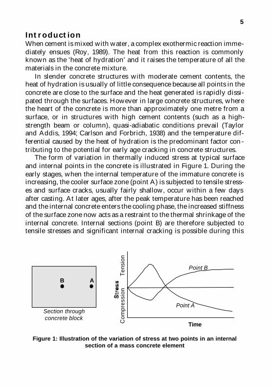
The form of variation in thermally induced stress at typical surfaceand internal points in the concrete is illustrated in Figure 1. During theearly stages, when the internal temperature of the immature concrete isincreasing, the cooler surface zone (point A) is subjected to tensile stress-es and surface cracks, usually fairly shallow, occur within a few daysafter casting. At later ages, after the peak temperature has been reachedand the internal concrete enters the cooling phase, the increased stiffnessof the surface zone now acts as a restraint to the thermal shrinkage of theinternal concrete. Internal sections (point B) are therefore subjected totensile stresses and significant internal cracking is possible during this

5

Figure 1: Illustration of the variation of stress at two points in an internalsection of a mass concrete element

Ten

sion

Com

pres

sion

Point B

Section throughconcrete block

Point A

Time

B A

period (Andersen, 1998). During this phase, the surface sections experi-ence compressive stress.

The purpose of this monograph is to provide designers of concretestructures with a basic numerical model for predicting time-temperatureprofiles in concrete elements during the early stages of hydration of thecementitious materials. The model is intended as a preliminary designtool and can be used to:• Provide an early assessment of the likely temperature profiles and

gradients in the structure as well as the time-based variations of theseprofiles;

• Select suitable binder type and binder content for the concrete to beused on the project

• Assess the impact of construction strategies such as artificial coolingof concrete constituents or placing concrete in different seasons, onthe likely temperature profiles in the structure.The model is based on a finite difference numerical solution of the

Fourier heat-flow equation and runs in a commercial spreadsheet(Ballim, 2004). Information on the rate of heat evolution of the cementi-tious binder in the concrete is obtained from laboratory-based adiabaticcalorimeter tests (Gibbon et al, 1997). The model uses this information asinput and typical heat rate curves for South African cementitious mate-rials are included in the model.

The development of stresses in the concrete and the potential forcracking are based on a complex interaction of temperature gradients,tensile strength, elastic modulus as well as creep and shrinkage capacity.All of these parameters change with time during the early stages ofhydration and it is beyond the scope of this monograph to deal withearly-age stress development in a complete manner.

The development of the model, its operation and limitations are cov-ered in the text of this monograph. The actual finite difference model,which runs as a Microsoft Excel® file is contained in the compact diskincluded with this monograph.

Development of the finite-difference temperature modelThe flow of heat in concrete is governed by the Fourier equation, whichin its two dimensional form is given as:

6

(1)

where: ? ? = density of the concreteCp = the specific heat capacity of the concreteT = temperaturet = timek = thermal conductivity of the concretex, y = the coordinates at a particular point in a structureq = the heat evolved by the hydrating cement

= is the time rate of heat evolution at point (x, y) in the structure.

Equation 1 is the transient form of the Fourier equation in that tem-perature at any point in the structure varies with time in first order form,as well as with position (x; y) in second order form. Also, the rate of heatevolution is required as input in the solution of Equation 1 and this termis time-dependent because the rate of hydration varies with time.Developing an appropriate form of the rate of heat evolution in concreteis discussed in more detail later.

The temperature prediction model presented in this monograph usesa finite difference numerical technique to solve Equation 1 for a rectan-gular block of concrete, which has a z dimension significantly longerthan the x and y dimensions. As shown in Figure 2, the block is cast ontoa rock foundation (thermal conductivity = kR) and the ambient air tem-perature (TA) varies with time.

Figure 2: Schematic arrangement of the modelled concrete block.

7

Concrete block

Time, TRock: k = k ; Temp = T = f(t)R R

Developing the node equationsThe numerical solution of Equation 1 is covered in a number of texts(Holman, 1990; Dusinberre, 1961; Croft and Lilley, 1977) and only thefinal form of the finite difference equations for the different situations inthe concrete block and associated boundary conditions are presentedhere. Figure 3 shows the different node positions for which the finite dif-ference equations were developed.

Note that points N, W, E and S are node points which are adjacent to (andexchange heat with) the point under consideration (point P)

Figure 3: Node positions and boundaries for the finite difference equations

The finite difference equations for each of the conditions shown in Figure3 are presented below.

Internal nodes (refer to Figure 3a)(2)

Subject to:

(3)

8

N N

a) P is an internal node

c) P is a corner node

b) P is a bottom node on rock

P

Ph h

PW

TA TA

WE

E

E

S

N

d) P is an exposed edge node

PW

SS

R = node in rock

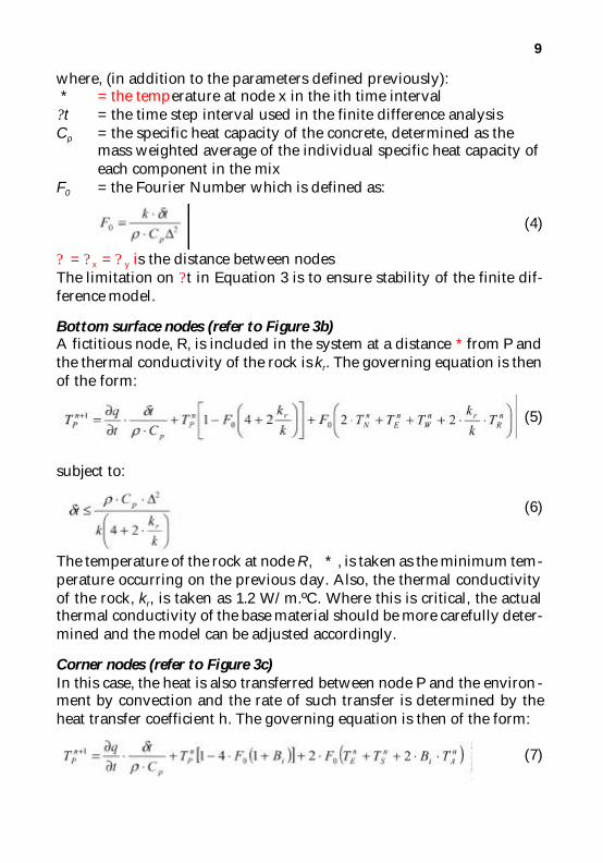
where, (in addition to the parameters defined previously):* = the temperature at node x in the ith time interval

?t = the time step interval used in the finite difference analysisCp = the specific heat capacity of the concrete, determined as the

mass weighted average of the individual specific heat capacity ofeach component in the mix

F0 = the Fourier Number which is defined as:

(4)

? = ? x = ? y is the distance between nodes The limitation on ?t in Equation 3 is to ensure stability of the finite dif-ference model.

Bottom surface nodes (refer to Figure 3b)A fictitious node, R, is included in the system at a distance * from P andthe thermal conductivity of the rock is kr. The governing equation is thenof the form:

(5)

subject to:

(6)

The temperature of the rock at node R, * , is taken as the minimum tem-perature occurring on the previous day. Also, the thermal conductivityof the rock, kr, is taken as 1.2 W/m.ºC. Where this is critical, the actualthermal conductivity of the base material should be more carefully deter-mined and the model can be adjusted accordingly.

Corner nodes (refer to Figure 3c)In this case, the heat is also transferred between node P and the environ -ment by convection and the rate of such transfer is determined by theheat transfer coefficient h. The governing equation is then of the form:

(7)

9

subject to:

(8)

where Bi is the Biot number and is defined as:

(9)

Exposed surface nodes (refer to Figure 3d)As for the corner nodes, heat is transferred to the environment and thefinite difference equation is:

(10)

subject to:

(11)

Modelling the environmental temperature TAAt the design stage of a construction project, it is unlikely that reliableambient temperature data are available for the area in which the con-struction is to take place. This is particularly true when temperature val-ues are required at approximately 1 hour intervals. However, daily ambi-ent maximum and minimum temperatures are usually easily availablefrom the local meteorological office. A model was developed to estimatethe ambient temperature at any time, using only the daily maximum andminimum values. This model takes the form:

(12)

where: td = the clock time of day at which the prediction is being made (0

to 24 hours)tm = the time at which the minimum overnight temperature occurs

(usually at sunrise)Tmax = the maximum temperature for the day under considerationTmin = the minimum temperature for the day under consideration

10

The model is fairly rough in that it ignores factors such as cloud cover,wind or direct sunlight and there is probably room for significant refine-ment. Nevertheless, Figure 4 shows that the model gives a reasonablygood prediction when compared with actual measured outdoor temper-atures over a period of approximately 10 days.

Figure 4: Measured air temperatures compared with the modelled valuesusing Equation 12

Determining the rate of heat evolution of the cementitious binderThe heat of hydration of cement can be determined by means of a test inan adiabatic calorimeter, such as the one described by Gibbon et al (1997)and illustrated schematically in Figure 5. Adiabatic testing is convenient,reproducible and practical. It has the added advantage that the test canbe conducted on a sample of the actual concrete to be used in the struc-ture.

In principle the test involves placing a 1litre sample of concrete,immediately after casting, in a water bath, such that a stationary pocketof air separates the sample from the water. The signal from a tempera-ture probe placed in the sample is monitored via an analogue to digitalconversion card by a personal computer which switches a heater in thewater bath on and off to maintain the water at the same temperature asthe concrete sample. This ensures that there is no exchange of heatbetween the concrete sample and the surrounding environment. Thepocket of air around the sample is important because it dampens any

11

0

5

10

15

20

25

Air

Te

mp

era

ture

(d

eg

. C

)

0 50 100 150 200 250 Time (hrs)

Measured Model

harmonic responses between the sample and the water temperatures asa result of the measurement sensitivity of the thermal probes. The test isusually run over a period of 7 days, by which time the rate of heat evo-lution is too low to be detected as a temperature difference by the ther-mal probes.

Figure 5: Schematic arrangement of an adiabatic calorimeter

The test produces a curve of temperature vs. time for a particularbinder type and mix composition. The total heat evolved at any time bya unit mass of cementitious binder can be determined from the relation-ship:

(13)

where:Cp = the specific heat capacity of the sample, is the change in tem-

perature of the sample over the time period under considerationms = the mass of the samplemc = the mass of cementitious material in the sample.

The rate of heat evolution can then be determined by means of numeri-cal differentiation with respect to time (t) of the total heat curve, i.e.:

(14)

An example of the total heat and heat rate curve for a ‘typical’ SouthAfrican cement, as measured in the Wits University adiabatic calorime-ter, is shown in Figure 6.

12

SampleHeater

Signal conditioningunit

PC with A/Dconversion

cardTemperature

probe

Air

Stirrer

Water

AC

Figure 6: Typical heat curves for a local Portland cement

However, the form of the heat rate relationship shown in Figure 6 isnot appropriate for use in solving the Fourier equation (Equation 1). Thisis because, as a chemical reaction, the rate of hydration of cement is alsotemperature dependent. The heat rate curve shown in Figure 6 thereforeonly applies to the unique temperature conditions under which the adi-abatic test was conducted. Since different points in a concrete structurecan be expected to experience different time-temperature histories, therate of heat evolution will vary at different points in the structure. Toaddress this problem, Ballim and Graham (2003) describe an approach inwhich the heat rate is expressed in maturity (or extent of hydration)form, rather than in clock-time form. The approach they proposes usesthe Arrhenius form of maturity, which can be written as (based on Naik1985):

(15)

Where:M = the equivalent maturity time as for a concrete cured at 20ºC,

expressed as t20 hours (see Figure 7 below)E = the activation energy parameter (33.5 kJ/mole) which is taken

as a constant (Bamford and Tipper, 1969)R = the universal gas constant (8.314 J/mole)Ti = the temperature in ºC at the end of the ith time interval ti = clock time at the end of the ith interval

13

Time (hours)

Total heat

Heat rate

400

300

200

100

0

6

5

4

3

2

1

00 20 40 60 80

The rate of heat evolution curve can therefore be normalised byexpression as a maturity rate of heat evolution:

This form of the heat rate curve can then be used as input for solution ofEquation 1. The time-based heat rate at each point in the structure at aparticular time of analysis is determined from the expression:

(16)

Equation 16 shows that, in the solution to Equation 1 for a concrete struc-ture, it is necessary to monitor the development of maturity as well asthe rate of change of maturity at each point under analysis in the struc-ture.

Figure 7 shows the heat curves for the Portland cement presented inFigure 6 above, but expressed in maturity form. In this maturity form,the heat rate curve is suitable for use in a numerical solution of Equation1.

Figure 7: Heat curves of Figure 6 expressed in maturity form.

Graham (2002) showed that the heat-rate profiles of South Africancements can vary significantly. Figure 8 shows the range of heat profilesfor nine South African cements tested in the adiabatic calorimeterdescribed above.

14

Time (t hours)20

Total heat

Heat rate

400

300

200

100

0

4

3

2

1

00 50 100 150 200 250

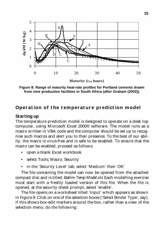
Figure 8: Range of maturity heat-rate profiles for Portland cements drawnfrom nine production facilities in South Africa (after Graham (2002)).

Operation of the temperature prediction model

Starting upThe temperature prediction model is designed to operate on a desk topcomputer, using Microsoft Excel 2000® software. The model runs as amacro written in VBA code and the computer should be set up to recog-nise such macros and alert you to their presence. To the best of our abil-ity, the macro is virus-free and is safe to be enabled. To ensure that themacro can be enabled, proceed as follows:

• open a blank Excel workbook

• select Tools; Macro; Security

• in the ‘Security Level’ tab, select ‘Medium’ then ‘OK’The file containing the model can now be opened from the attached

compact disc and is titled: Ballim Temp Model.xls. Each modelling exercisemust start with a freshly loaded version of this file. When the file isopened, at the security check prompt, select ‘enable’.

The file opens on a worksheet titled ‘Input’ which appears as shownin Figure 9. Click on one of the selection boxes (‘Select Binder Type’, say).If this shows box-edit markers around the box, rather than a view of theselection menu; do the following:

15

0

1

2

3

4

5

0 10 20 30 40 50

Maturity (t 2 0 hours)

dq/d

M (

W/k

g)K

F

A

B

EH

G

D C

• deselect the box by clicking on another cell

• select View; Toolbars; Control Toolbox

• in the Control Toolbox, click on the ‘Design Mode’ icon (the onewith a set square, ruler and pencil). This toggles between the ‘Edit’and ‘Operate’ modes of the selection boxes.

• close the Toolbox by clicking on the ‘x’Data should only be entered in the blue areas and selections should

be made from the three drop-down menus. There are two other work-sheets entitled ‘Analysis’ and ‘Results’ which the user should not nor-mally need to access at the model set-up stage. The section below dis-cusses data entry in more detail.

Concrete details sectionThis section calls for details of the actual concrete being considered forthe structure. The mass of the different concrete components should beadded in the blue areas. In this case, the admixture content refers to liq-uid admixtures. The mass of powder chemical admixtures should beadded to the sand content.

These quantities are used to calculate the density of the concrete (asthe sum of the component masses) and the specific heat capacity of theconcrete. The specific heat capacity is taken as the weighted average ofthe specific heats of the solid materials (taken as 900 J/kg.ºC) and that ofthe water and liquid admixture (taken as 4190 J/kg.ºC).

Binder type selectionThe software allows a selection of one binder type from a list of sevenbinders. This sets up the measured maturity heat-rate profile for thebinder type selected. The selection includes a typical South African CEMI, three blends of this CEM I with ground granulated blast furnace slag(GGBS) and three blends of the CEM I with fly ash (FA). Users wishingto run the model with a different heat-rate profile should contact theauthors at the contact details given at the end of this monograph. Whena binder type selection is made, the red note on the lower right of thescreen will turn off.

Aggregate type selectionThe main purpose of this selection is to assign a value of the thermal con-ductivity of the concrete. Concrete thermal conductivity is strongly influ-

16

17

Figure 9: Appearance of the Input worksheet for data entry before running themodel

enced by the aggregate type and the software allows a selection from thelist of aggregates shown in Table 1. This table also shows the thermalconductivity values that are assigned to the concrete for use in themodel. These values have been adapted from those presented by vanBreugel (1998).

Table 1: Aggregates types included in the software and correspondingthermal conductivity values.

Aggregate type Thermal conductivity(W/m.ºC)

Quartzite 3.5

Dolomite 3.2

Limestone 3.1

Granite 2.7

Rhyolite 2.2

Basalt 2.1

It should be noted that there can be a range of thermal conductivity val-ues for aggregates which are nominally the same. The values presentedin Table 1 are ‘average’ values and, as with other parameters, are intend-ed to provide a first estimate of the temperatures in the structure.

Again, when an aggregate type selection is made, the red note on thelower right of the screen will turn off.

Construction details sectionConcrete casting timeThis is the time of day at which the concrete is cast, using a 24-hour clock(e.g. 4.00 pm should be entered as 16). This value is required in usingEquation 12 to estimate the ambient temperature at each time interval inthe analysis.

Concrete casting temperatureThis is the initial temperature of the concrete at the time of casting. Thisvalue will appear as the temperature at all nodes in the time t=0 block ofthe results sheet after the model is run.

The initial temperature of the concrete is an important design andconstruction variable which can be used to control the temperature pro-

18

files in the concrete. Strategies to cool the aggregates or using chilledwater as mix water are effective ways to reduce the initial temperature ofthe concrete. In the absence of a more direct measurement, the initialtemperature of the concrete can be estimated from the mass and specificheat weighted average as shown in Equation 17.

(17)

where:Tc = the temperature of the concrete mixture;mi = mass of the ith component of the concrete (cement, sand, stone,

water, …)Cpi = specific heat capacity of the ith componentTi = temperature of the ith component at the time it is introduced

into the mixer.The specific heat capacity of the solid materials can be taken as 900J/kg.oC and that of the water and liquid admixture can be taken as 4190J/kg.oC.

Formwork typeThis is selected from a drop-down menu which has only two selections:timber or steel. This information is necessary to select the appropriatevalues for the heat transfer coefficient (h in Equations 9 and 11). Themodel uses a value of 25 W/m2.ºC for all exposed concrete surfaces. Thisvalue is appropriate for light wind weather conditions. While the sidesurfaces are covered with formwork, an h value of 5 W/m2.ºC is used ifthe formwork is timber, or 25 W/m2.ºC if steel formwork is used. If noformwork selection is made, the programme defaults to timber form-work. It is assumed that the top surface of the concrete is not covered byany formwork.

Concrete age at formwork removalAs discussed above, this value is used to determine the time at which thevalue of h should be changed to the exposed value for the side surfacesof the structure.

19

Maximum and minimum day temperaturesThese values are necessary to estimate the ambient temperature at dif-ferent times during the day using Equation 12. In solving this equation,the model takes tm, the time at which the minimum temperature occurs,as 06h00.

Structure and analysis details sectionHorizontal and vertical dimensions of the structureThese are the overall dimensions of the structure and set the limits forthe node positions in the model analysis. For a rectangular prismaticstructure, the smaller of the two horizontal dimensions should be usedas this will represent the direction of steepest temperature gradients.

Space interval (?x = ?y = ? ) for analysisThis value determines the spacing of the nodes to be used in the finite-difference analysis. The model temperature predictions will be calculat-ed and reported at each of these nodes. The overall dimension of thestructure should be whole number multiples of the space interval select-ed. If this is not so, the model will extend the overall dimension of thestructure to the next nearest node position. There are a few limitations onthe value of the space interval selected:• There should be more than 3 nodes in both directions

• There should be less than 26 nodes in the x direction and less than 39nodes in the y direction

• For a particular selection of the space interval, the time intervalshould be small enough to satisfy the conditions set by Equations 3,6, 8 and 11.

If a value for the space interval is entered and one or more of the condi-tions mentioned above are not satisfied, an appropriate warning willappear in one of the cells below the ‘Structure and Analysis Details’ box.A different value of space interval should be selected until this warningmessage is cleared.

Time interval for analysisThis is the ?t used in the model and represents the concrete age intervalsat which the analysis is undertaken and temperature results reported.The most important limitation on the time interval is that it should sat-isfy the conditions set by Equations 3, 6, 8 and 11. If a time interval isselected which does not satisfy all these conditions, an appropriate

20

warning will appear in one of the cells below the ‘Structure and AnalysisDetails’ box. A smaller value of time interval (or different value of spaceinterval) should be selected until this warning message is cleared. Themodel does allow factions of an hour to be used and it is good practiceto use a time interval of 4 hours or less.

Time duration of analysisThis is the time or concrete age over which the analysis is to be under-taken. The number of time cycles of analysis that will appear in theresults sheet is the time duration divided by the time interval selected.

Running the modelAfter the data fields have been completed in the ‘Input’ worksheet andthe appropriate selections have been made, hold down the ‘ctrl’ buttonand press ‘h’ to run the model. At the end of the model run, the‘Analysis’ and ‘Input’ worksheets are deleted and the top of the ‘Results’worksheet is displayed.

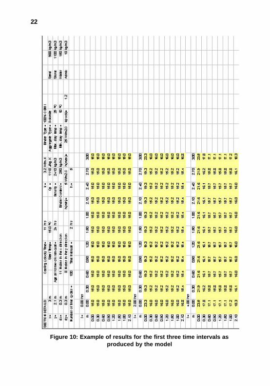
The top of the ‘Results’ worksheet shows the basic data that was usedin the analysis. Temperature predictions are shown at each node for suc-cessively increasing time intervals. Figure 10 shows the first three blocksof results in the analysis of a concrete element measuring 3 m x 2.1 m.The casting temperature of the concrete is 15ºC and the analysis wasundertaken in space intervals of 0.3 m with time intervals of 2 hours.

Saving and analysing the resultsAfter the model run, it is important that the results be saved under a newfile name using the ‘Save As’ facility. Saving the file without changingthe file name may overwrite the master analysis file. Also, the file stillcontains the macro used for the model analysis but this will no longeroperate as a temperature prediction model. It is advisable to delete thismacro using the ‘Tools; Macro …’ facility.The user can now interrogate the data in the ‘Results’ worksheet to con -sider the time-temperature profiles at different points in the structure.Predicted temperatures at particular points in the structure can also beextracted and compared with temperatures at other points in order todetermine the likely temperature gradients in the structure.

21

22

Figure 10: Example of results for the first three time intervals as produced by the model

Closure The method described in this monograph provides a simple and reason -ably accurate method for predicting temperatures in concrete elementsduring the early stages of hydration. The model has been structured tobe applicable in a wide range of applications. Heat rate data for a typicalCEM I and various combinations of FA and GGBS are included in themodel.

It must be emphasised that this model was developed as a prelimi-nary design and construction tool and should be used to provide initialestimates of the temperature profiles that are likely to occur in a largeconcrete element.

The authors welcome any suggestions for improvement of the modelor considerations of particular applications for which the parametersincluded in the model may not be appropriate. We would also appreci-ate any in situ measurements of concrete temperature which could beused to further verify the model. Please send communications to:

Prof. Yunus Ballim School of Civil & Environmental EgineeringUniversity of the WitwatersrandPrivate Bag 3, Wits, 2050, South AfricaTel: (+2711) 717-7103;Fax: (+2711) 339-1762e-mail: ballim@civil.wits.ac.za

Finally, this monograph and the included software are issued withoutany charge. Please include an appropriate acknowledgement if theresults of the model are used in any formal documentation.

ReferencesAndersen, ME (1998). Design and construction of concrete structures using tem-

perature and stress calculations to evaluate early-age thermal effects. In:Materials Science of Concrete V, Skalny, J and Mindess, S (Eds).American Ceramic Society, Westerville, Ohio.

Ballim, Y and Graham, PC (2003). A maturity approach to the rate of heat evo-lution in concrete. Magazine of Concrete Research vol. 55, No. 3, pp. 249-256

Ballim, Y (2004). Temperature rise in mass concrete elements – Model develop-ment and experimental verification using concrete at Katse dam. Journal ofthe SAICE, vol. 46, No. 1, pp. 9-14

23

Bamford, C. H. and Tipper, C. F. H. (eds.) (1969). Comprehensive chemicalkinetics , Vol. 1: The practice of kinetics. Elsevier Publishing Company,London.

Carlson, RW and Forbrich, LR (1938). Correlation of methods for measur-ing heat of hydration. Industrial and Engineering Chemistry (USA), Vol.10, No. 7, pp: 382-386.

Croft DR and Lilley DG (1977). Heat transfer calculations using finite differ-ence equations. Applied Science Publishers Ltd., London. 283 pgs.

Dusinberre GM (1961). Heat transfer calculations by finite differences.International Textbook Company, Pennsylvania, US. 293 pgs.

Gibbon, GJ., Ballim, Y. and Grieve, GRH (1997). A low-cost, computer-con-trolled adiabatic calorimeter for determining the heat of hydration of concrete.ASTM Jnl. of Testing and Evaluation, 25, No. 2, pp. 261-266.

Graham, PC (2003). The heat evolution characteristics of South African cementsand the implications for mass concrete structures. PhD Thesis submitted tothe University of the Witwatersrand.

Holman, J. P (1990). Heat transfer, 7th Ed. McGraw Hill Inc. New York.Naik T.R (1985). Maturity functions for concrete during winter conditions. In:

Temperature Effects on Concrete, ASTM STP 858, T.R. Naik, Ed.,American Society for Testing and Materials, Philadelphia.

Roy, DM (1989). Fly ash and silica fume chemistry and hydration. In: Proc. of3rd International Conference on Fly Ash, Silica Fume, Slag and NaturalPozzolans in concrete. Malhotra, VM (Ed). ACI SP-114. AmericanConcrete Institute, Detroit.

Taylor, PC and Addis, BJ (1994). Concrete at early ages. In: Fulton’s ConcreteTechnology, 7th Edition, Portland Cement Institute, Midrand, SouthAfrica.

van Breugel, K (1998). Prediction of temperature development in hardening con-crete. In Prevention of Thermal Cracking in Concrete at Early Ages.Springenschmid, R (ed.), Rilem Report 15. Chapter 4. E&FN Spon,London, pp. 51-75.

24