Embed Size (px)
Citation preview
A numerical algorithm for zero counting.
IV: An adaptive speedup
Josue Tonelli-Cueto∗
Inria Paris & IMJ-PRGSorbonne Universite
Paris, [email protected]
Abstract
In this paper, we provide an adaptive version of the algorithm for counting realroots of real polynomial systems of Cucker, Krick, Malajovich and Wschebor. Weshow that, unlike the original algorithm, the adaptive version runs in finite expectedtime, while preserving the good properties of the original: numerically stable, highlyparallelizable and good probabilistic run-time. Moreover, our probabilistic complexityanalysis will be robust not limiting itself to KSS random polynomial systems.
1 Introduction
The trilogy of papers A numerical algorithm for zero counting [26, 27, 28] by Cucker,Krick, Malajovich and Wschebor is the first milestone of the so-called grid method [21, 22].Their algorithm, from now on CKMW, is numerically stable, highly parallelizable and has agood run-time with high probability. The latter still holds under very general probabilisticassumptions [36, 37]. So, as with many trilogies in the last decade, we must answer thequestion: why does this classic trilogy need a sequel?
In one sentence: CKMW has infinite expected run-time (even for KSS polynomial sys-tems). The shadow of this fact affects subsequent descendants of CKMW for computing thehomology of real smooth projective varieties [29], basic semialgebraic sets [13] and generalsemialgebraic sets [15, 16] (cf. [76]). In this way, we cannot hope for finite expected run-times for the latter problems if we don’t have such finite expected run-time for the mostsimple problem: counting real zeros.
In this sequel paper, we present an adaptive version of CKMW, which we call aCKMW,whose run-time has finite expectation, and that preserving all the nice properties of theoriginal algorithm: numerical stability, highly parallelizability, and good probabilistic run-time. Our result is an step towards the holy grail of real numerical algebraic geometry: anumerical algorithm for computing the homology groups of semialgebraic sets in expectedsingle exponential time. Unfortunately, our results are not enough to solve this problem.
Without more hesitation, let’s state our main result in an informal way. To see the fulltechnical version, see Theorem 2.21 in the next section where we explain in full technicaldetail all the claims of the theorem.∗This work and the author were supported by a postdoctoral fellowship of the 2020 “Interaction”
program of the Fondation Sciences Mathematiques de Paris. Partially supported by ANR JCJC GALOP(ANR-17-CE40-0009), the PGMO grant ALMA, and the PHC GRAPE.
1
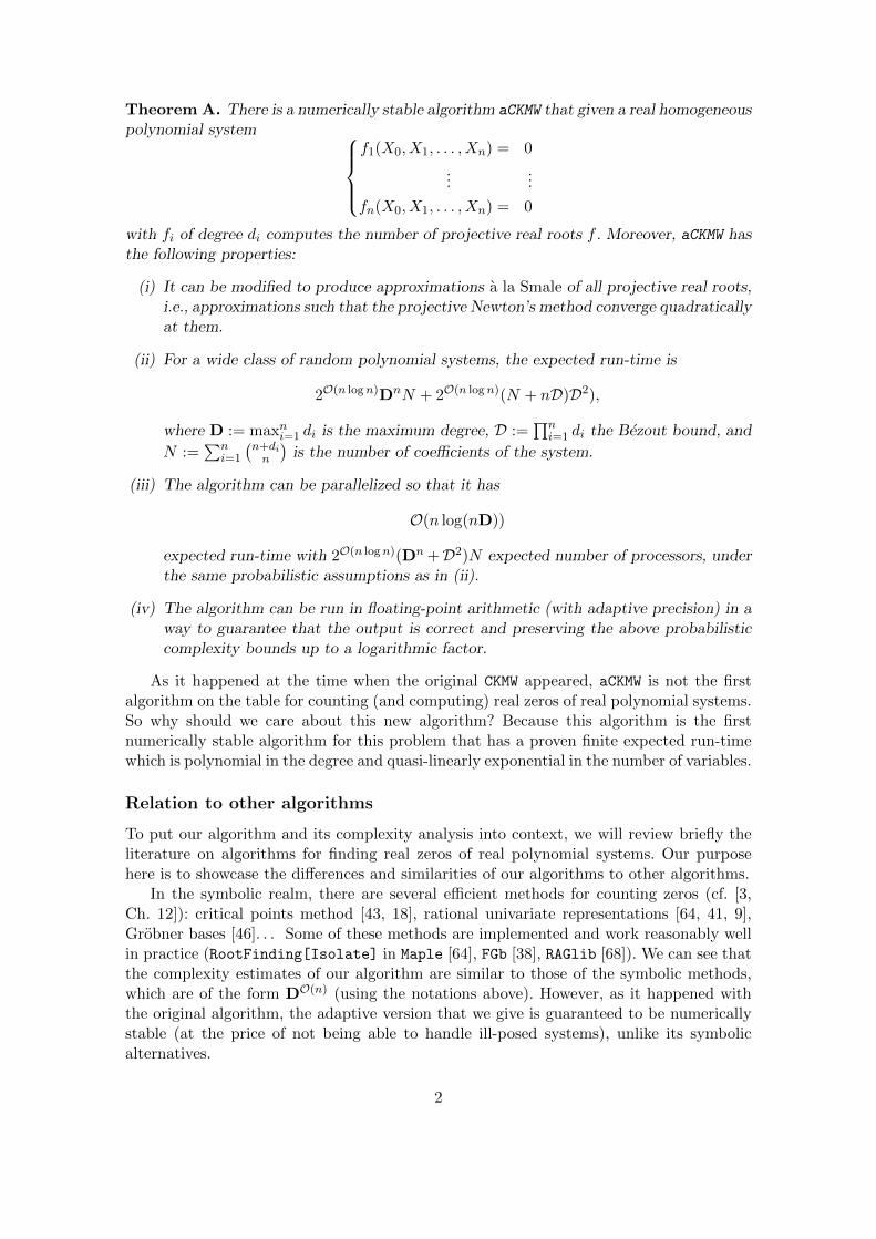
Theorem A. There is a numerically stable algorithm aCKMW that given a real homogeneouspolynomial system
f1(X0, X1, . . . , Xn) = 0
......
fn(X0, X1, . . . , Xn) = 0
with fi of degree di computes the number of projective real roots f . Moreover, aCKMW hasthe following properties:
(i) It can be modified to produce approximations a la Smale of all projective real roots,i.e., approximations such that the projective Newton’s method converge quadraticallyat them.
(ii) For a wide class of random polynomial systems, the expected run-time is
2O(n logn)DnN + 2O(n logn)(N + nD)D2),
where D := maxni=1 di is the maximum degree, D :=∏ni=1 di the Bezout bound, and
N :=∑n
i=1
(n+din
)is the number of coefficients of the system.
(iii) The algorithm can be parallelized so that it has
O(n log(nD))
expected run-time with 2O(n logn)(Dn +D2)N expected number of processors, underthe same probabilistic assumptions as in (ii).
(iv) The algorithm can be run in floating-point arithmetic (with adaptive precision) in away to guarantee that the output is correct and preserving the above probabilisticcomplexity bounds up to a logarithmic factor.
As it happened at the time when the original CKMW appeared, aCKMW is not the firstalgorithm on the table for counting (and computing) real zeros of real polynomial systems.So why should we care about this new algorithm? Because this algorithm is the firstnumerically stable algorithm for this problem that has a proven finite expected run-timewhich is polynomial in the degree and quasi-linearly exponential in the number of variables.
Relation to other algorithms
To put our algorithm and its complexity analysis into context, we will review briefly theliterature on algorithms for finding real zeros of real polynomial systems. Our purposehere is to showcase the differences and similarities of our algorithms to other algorithms.
In the symbolic realm, there are several efficient methods for counting zeros (cf. [3,Ch. 12]): critical points method [43, 18], rational univariate representations [64, 41, 9],Grobner bases [46]. . . Some of these methods are implemented and work reasonably wellin practice (RootFinding[Isolate] in Maple [64], FGb [38], RAGlib [68]). We can see thatthe complexity estimates of our algorithm are similar to those of the symbolic methods,which are of the form DO(n) (using the notations above). However, as it happened withthe original algorithm, the adaptive version that we give is guaranteed to be numericallystable (at the price of not being able to handle ill-posed systems), unlike its symbolicalternatives.
2
In the numerical realm, homotopy continuation is the queen. To solve the consideredproblem, the main path would be to compute all the complex roots and then counts thereal ones. To compute all the complex zeros, there are many ways: total degree homo-topy [63] (cf. [12, 18.4.1]), real homotopies [55], repeatedly computing one random rootuntil roots are obtained [5, §10.2], monodromy [33]. . . The majority of these methodsare implemented in many ways (PHCpack [78], Bertini [4], NAG4M2 [54] Hom4PS-3 [19],juliahomotopy.jl [11]) and perform very well in practice. Moreover, one can even cer-tify the final count of real zeros efficiently in practice using floating-point interval arith-metic [67, 53, 10] (cf. [59, Ch. 5]), or using the not so efficient rational arithmetic [47].
However, despite all the progress in numerical complexity theory on solving complexpolynomial systems through homotopy continuation [12, III], the full resolution of theoriginal Smale’s 17th problem [51] and theoretical achievements beyond its scope [52, 14],the numerical complexity of finding the real zeros (or finding just one complex zero) ofreal polynomial systems through homotopy continuation (or any other numerical method)remains a widely open problem1. Hence, by means of our algorithm and its complexityanalysis, we show for the first time that the problem of computing the real zeros of a realpolynomial system can be solved numerically in finite expected time. In the future, weshould aim at improving our complexity-theoretical knowledge of homotopy continuation,so that homotopy continuation becomes the complexity-theoretical queen also in the realmof real numerical algebraic geometry.
In the so-called symbolic-numerical realm, the class of relevant algorithms is thoseknown as subdivision methods. In the univariate setting, subdivision methods are nearoptimal to compute the real roots of real univariate polynomials [60, 69] (cf. [50]). In themultivariate case, there are not near optimal algorithms and one must consider a larger zooof subdivision methods. The simplest ones are based on some interval version of Newton’smethod [59, Ch. 5] or some test based on Miranda’s theorem [80], which work not only forpolynomials, but any C1-function with simple zeros. A more sophisticated class exploitsthe Bernstein basis to exclude roots using linear programming [70], normal cones [35] orreduction-to-one-dimension techniques [58], and for including roots they exploit Miranda’stheorem [39, 40]. We note that subdivision methods based in reduction techniques can beextended to more general functions [77] and to polynomials in the monomial basis [57].In practice, these algorithms work reasonably well (see, in addition to the mentionedreferences, GlobSol [48], INTLAB [66] and IntervalRootFinding.jl [7]). However, thecomplexity of these algorithms is not well understood [81, p. 32]. In the cases where acomplexity analysis is available, the complexity estimates seem to depend on quantitiesthat are either unknown or hard to interpret (e.g. ND(f) in [58, Theorem 5.7], the cost ofthe oracles in [57, Proposition 5.2.] or the λs in [80, §7]).
Anyone familiar with these subdivision methods described in the previous paragraphwill notice that aCKMW is very similar to a subdivision method. This similarity is not sur-prising as the underlying idea of the grid method (i.e., approximate the space with a cloudof points to capture an object in it) is ‘dual’ to that of subdivision methods (i.e., subdividethe space into smaller regions). In particular, our algorithm is very similar to those sub-division methods of [59, Ch. 5], but it uses a variation of Smale’s α-theory [74] (cf. [31])instead of interval versions of Newton’s method. In other words, our algorithm does notuse any fancy methods beyond Newton’s method in it. We note that our complexity anal-ysis of aCKMW is better than the ones existing for subdivision methods in two ways: 1) the
1Up to the knowledge of this author and without considering papers related to the grid method, [8] and[61] are the only existing works considering the numerical complexity of solving real polynomial systems.
3
condition-based estimate is easy to interpret, and 2) the probabilistic estimate allows usto understand how the algorithm works in practice. We think that this kind of complexityanalysis might help in understanding theoretically and not only in practice the subdivisionmethods.
Background, techniques and achievements
The core of the paper is to make the algorithm CKMW adaptive and analyze the complexityby taking this into account. However, the ideas of this paper didn’t generate ex nihilo.Here, we describe briefly what was known and what this paper brings to the table in termsof techniques of complexity analysis.
The idea that an adaptive grid method might provide acceleration was already in theair when CKMW was proposed in [26]. However, there were two main obstacles: 1) how tofind an efficient procedure to make the grid method adaptive, and 2) how to exploit theadaptive nature to the algorithm to obtain a better complexity estimate.
The existence of complexity analyses that could take advantage of the latter becameclear while analyzing the complexity of the Plantinga-Vegter algorithm in [23] (cf. [25]).In this work, the continuous amortization technique of [17] made it clear that, for theadaptive grid method, the condition-based bound of the run-time should be in terms ofan expression of the form
Ex∈Snκ(f, x)n, (1.1)
where κ(f, x) is a local condition number measuring how near is f of being ill-posedaround x. This ‘averaged-over-the-sphere’ expression contrasts with the ‘supremum-over-the-sphere’ expression,
supx∈Sn
κ(f, x)n, (1.2)
used to bound the run-time of all previous algorithms based on the (non-adaptive) gridmethod. The change from (1.2) to (1.1) has important probabilistic consequences. While(1.2) does not have finite expectation2 when we randomize f , (1.1) does indeed have finiteexpectation.
The above change in the bound can be seen as a real analogue of the change fromnon-adaptive homotopy to adaptive homotopy done by Shub [71] in complex numericalalgebraic geometry. In the complex setting, this change meant passing from infinite vari-ance to finite variance for the run-time of homotopy continuation [6]. As we have seenabove, in the real setting, the change is more dramatic as we pass from infinite expectedrun-time to finite run-time. However, as it happened with [71], the above change does notcome with an adaptive grid method.
The first construction of an algorithm using an adaptive grid method was done byHan [44, 45]3, but his algorithm has two major flaws: 1) it is not constructive, and 2) thebound of its run-time involves
Ex∈Snκ(f, x)2n, (1.3)
which does not have a finite expectation when we randomize f . Again, unlike in thecomplex setting, the real setting demands extra care. One can make a constructive grid
2Note that in previous works, one goes around the fact that (1.2) does not have finite expectation usingvariation of the notion of weak complexity [2]. In this way, one says that (1.2) is sufficiently small withhigh probability.
3We warn the reader about the numerous mistakes of these references. This means that any statementcan be false beyond trivial corrections.
4
method, as done by the author in [76, Ch. 4§3] to show that one can estimate (1.2) infinite expected time4. Building on this work, Eckhardt [34] proposes a fully constructiveversion of Han’s adaptive algorithm for computing the homology of basic semialgebraicsets5. Unfortunately, Eckhardt’s algorithm’s run-time’s bound still involves (1.3), whichdoes not have finite expectation (with respect a random f).
Hence, after all these developments, one can see that obtaining an adaptive grid methodthat works in finite expected time is non-trivial. The main reasons for this are the following:
(1) The procedure to select an approximating cloud of points from the adaptive grid seemsto require a quadratic condition in κ(f, x). The latter is enough to force (1.3) into thecomplexity estimates.
(2) The post-processing step of the approximating cloud of points has to be done in away that it avoids pairwise comparisons among all points. If pairwise comparisons,or even worse, k-subset comparisons as it required for current homology computingalgorithm, are required, the naive complexity estimates will be at quadratic in (1.1).A priori, we don’t expect squares of (1.1) to behave a lot more differently than (1.3),and, in particular, to have finite expectations.
In general, the post-processing step is the hardest part of subdivision methods. For ex-ample, although one might think that the analysis here is similar to the one done for thePlantinga-Vegter algorithm [23] (cf. [25]), we note that there we didn’t deal with the selec-tion or processing step. Dealing with them in a way that the complexity estimates don’tblow up can be a challenging problem. In particular, for the Plantinga-Vegter algorithmthis is so due to the need of very exact sign evaluations [81, p. 32].
In this paper, we solve these two issues for zero counting. For (1), we recover the useof Smale’s β in Smale’s α-criterion without using bounds of the form
β(f, x) ≤ µ(f, x)‖f(x)‖‖f‖W
, (1.4)
which were the ones responsible for the quadratic condition in (1). The reason this changeworks is because we can guarantee that β(f, x) is small, and so that Smale’s α-criterionis satisfied, if x is near enough a root. For (2), we use strongly that the topology of azero dimensional set is discrete. Now, doing this alone is not enough for the bounds inTheorem A. For this, we need to incorporate several tricks:
• Change of norm: Instead of using the Weyl norm ‖ ‖W , we use the real L∞-norm‖ ‖∞ following the ideas in [24]. Doing this, allows us to have N instead of Nn+1 isthe estimate of the expected run-time.
• Row normalization of the systems: We normalize our polynomial system, equationby equation. In other words, instead of normalizing f as f/‖f‖∞, we normalize it as(fi/‖fi‖)i. This substitutes a D2n factor is the estimate of the run-time by D2 thesignificantly smaller.
• Lipschitz-constant-decreasing normalization of condition: Instead of dealing with lo-cal condition numbers κ(f, x) that are D-Lipschitz in x (2nd Lipschitz property), we
4This publication is the first one containing results related to that part of the PhD thesis of the author.5Let us note that the work of Eckhardt was highly non-trivial, as it had to provide completely new
lower bounds for the local reach of a basic semialgebraic sets in [44, 45] are completely wrong.
5
introduce additional normalization by the diagonal matrix of degrees ∆ to force thisfunctions to be 1-Lipschitz in x. As the operation above, this allows us to transformseveral Dn in the estimates by D.
We note that the factor Dn comes from the need to compute ‖ ‖, but this computationcan be avoided at the price of turning aCKMW into a Montecarlo algorithm.
In the future, one should expect to extend the adaptive grid method to the computationof homology of algebraic and semialgebraic sets. The ideas exposed here generalize easily tosolve (1) for this problem (at least in the algebraic setting). The main challenge remains inthe solution of (2) when we cannot rely on the zero set being a discrete set. An alternativeline of work is to consider the original application of the grid method into feasibilityproblems [30, 20], whose complexity continues open [12, P.18].
Structure of the paper
In the next section, we explain in full detail the content of our algorithm, the probabilisticassumptions and all the complexity estimates. Then in Section 3, we provide all the resultsfor the variation of Smale’s α-theory that we will be using; in Section 4, we analyze thecondition-based and probabilistic complexity of the algorithm; and in section 6, we discussbriefly the finite precision of the algorithm.
2 Main Ingredients and Overview
Let n, q ∈ N, d := (d1, . . . , dq) ∈ Nq,
Hn,di := {g ∈ R[X0, . . . , Xn] | g is homogeneous of degree di},
the set of real homogeneous polynomials of degree di in X0, . . . , Xn, and
Hn,d[q] :=
q∏i=1
Hn,di = {f ∈ R[X0, . . . , Xn]q | for all i, fi is homogeneous of degree di},
the set of polynomial q-tuples f such that fi is an homogeneous polynomial of degree diin X0, . . . , Xn. We also introduce the following matrix
∆ = diag(d) =
d1 . . .
dq
∈ Rq×q. (2.1)
Associated to the above object, we consider the following constans:
• D := ‖d‖∞ = maxqi=1 di, the maximum degree.
• D :=∏qi=1 di ≤ Dq, the Bezout bound.
• N :=∑q
i=1
(di+nn
)≤ q(1 + D)n, the input size.
Given f ∈ Hn,d[q], we will consider the following notations:
• ∂kf ∈ R[X0, . . . , Xn]q×(n+1)⊗k is the tensor whose entries are given by the polyno-
mials ∂k
∂Xj1 ·∂Xjkfi. Note that given v1, . . . , vk ∈ Rn+1, ∂kf(v1, . . . , vk) is a q-tuple of
homogeneous polynomials (such that the ith component is of degree max{0, di−k}).
6
• ∂kxf is the value of ∂kf at x ∈ Rn+1.
• Dxf : TxSn → Rq is the tangent map of f (as a map on the sphere) at x ∈ Sn. Byabuse of notation, we will write Dxf = ∂xf(I− xx∗) for x ∈ Sn.
In what follows, we will describe the algorithm and the complexity results of this paper.Before that, we will introduce the main ingredients.
2.1 Main Ingredients
The main ingredients for our algorithm are the following ones: the L∞-norm, the conditionnumber, the δ-theory, and an adaptive grid. We will mainly do the exposition working onthe sphere Sn, as it is conceptually simpler. However, we note that all the relevant resultscan be adapted to the projective space, as the majority of the definitions are representative-invariant.
2.1.1 L∞-norm and exclusion lemma
In previous works in real numerical algebraic geometry, the usual norm to use was theWeyl norm. The Weyl norm of f ∈ Hn,d[q] is given by
‖f‖W :=
√√√√∑i
∑|α|=di
(diα
)−1f2i,α
where fi =∑|α|=di fi,αX
α. The disadvantage of this norm is the appearance of factors
of the form NO(n) in the complexity estimates of the algorithms. This can be avoided asshown in [24] by using other norms, such as the L∞-norm. The L∞-norm of f ∈ Hn,d[q]is given by
‖f‖∞ := maxx∈Sn
‖f(x)‖∞ = maxx∈Sn
maxi|fi(x)|.
We note that this norm is invariant not only under the action of the orthogonal groupO(n+1) on Hn,d[q], but also under the action of O(n+1)d on Hn,d[q]. The following resultby Kellogg [49, Theorem IV] (which we cite in the form given in [24, Corollary 2.20]) willbe the most useful result for us.
Theorem 2.1 (Kellogg’s Theorem). Let f ∈ Hn,d be an homogeneous polynomial ofdegree d. Then for all k ∈ N, x ∈ Sn and v1, . . . , vk ∈ Rn+1,∣∣∣∣ 1
k!∂kxf(v1, . . . , vk)
∣∣∣∣ ≤ (dk)‖f‖∞‖v1‖2 · · · ‖vk‖2.
In particular, f : Sn → R is d‖f‖∞-Lipschitz (with respect both the geodesic and Euclideanmetrics in Sn).
The above theorem can be applied component by component to f ∈ Hn,d[q] in orderto obtain an analogue of the exclusion lemma [26, Lemma 3.1]. Given f ∈ Hn,d[q], therow-normalization of f is the following polynomial tuple
f := (fi/‖fi‖∞)i ∈ Hn,d[q]. (2.2)
Note that the row-normalization is better than the naive normalization f/‖f‖∞, becauseit makes all polynomials of the same magnitude.
7
Proposition 2.2 (Exclusion lemma). Let f ∈ Hn,d[q]. Then ∆−1f : Sn → [0, 1] is awell-defined 1-Lipschitz map (with respect both the geodesic and Euclidean metrics onSn). In particular, for x ∈ Sn such that f(x) 6= 0,
BS
(x,∥∥∥∆−1f(x)
∥∥∥∞
)does not contain any zero of f .
The above result will allow us to exclude points that are very far away from the zeroset of f .
Remark 2.3. We note that [26] used originally the norm maxi ‖fi‖W because it was friendlyto the ∞-norm. Our choice for the L∞-norm has this advantage, with the addition of abetter probabilistic behaviour.
2.1.2 (Re-scaled) condition number
Given f ∈ Hn,d[q] and x ∈ Sn, the usually used condition numbers in numerical algebraicgeometry are
µ(f, x) := ‖f‖W∥∥∥Dxf
†∆12
∥∥∥2,2
and κ(f, x) :=(‖f(x)‖22/‖f‖2W + µ(f, x)−2
)− 12 ,
where A† := A∗(AA∗)−1 is the pseudoinverse, µ(f, x) = ∞ if Dxf is not surjective (byconvention), and ‖ ‖2,2 is the induced norm with the Euclidean norm ‖ ‖2 in both thedomain and codomain. The µ-condition number controls the conditioning of f around aroot x, the κ-condition number controls the conditioning of f around any point x. Becauseof this, the µ-condition number tends to appear in the complex setting and the κ-conditionnumber in the real one.
In [24, §3], these norms are adapted to the L∞-norm by changing ‖f‖W by√q‖f‖∞
and ∆12 by ∆. However, the scaling kept still favors the geometric approach of [12, Ch. 14]
instead of a more complexity-focused approach. To correct this, we introduce the followingvariant of the µ-condition.
Definition 2.4. Let f ∈ Hn,d[q] and x ∈ Sn. The ν-condition number of f at x is thequantity given by
ν(f, x) := ‖f‖∞∥∥∥D−1x f †∆2
∥∥∥∞,2
,
where ‖ ‖∞,2 is the operator norm with the ∞-norm in the domain and the Euclideannorm in the codomain, if Dxf is surjective, and ∞, otherwise.
Remark 2.5. Note that for the row-normalization of f , we have ν(f , x) =∥∥∥D−1x f †∆2
∥∥∥∞,2
.
The importance of the ν-condition lies in its use for controlling Newton’s methodthrough the means of δ-theory. We discuss this in the following point. The theorem belowshows the so-called Lipschitz properties of ν (term introduced in [76]). We note that ourchoice of scaling is so that the 2nd Lipschitz property has constant one. We postpone itsproof until Section 3.
Theorem 2.6. Let f ∈ Hn,d[q] and x ∈ Sn. Then the following holds:
8
• 1st Lipschitz property. For all g, g ∈ Hn,d[q],∣∣∣∣ ‖g‖∞ν(g, x)− ‖g‖∞ν(g, x)
∣∣∣∣ ≤ ‖∆−1(g − g)‖∞.
In particular, ν(f, x) ≥ 1.
• 2nd Lipschitz property. The map
Sn → [0, 1]
x 7→ 1
ν(f, x)
is 1-Lipschitz.
The condition number that will play a role in controlling the complexity around eachpoint will be the following one.
Definition 2.7. Let f ∈ Hn,d[q] and x ∈ Sn. The C-condition number of f at x is thequantity given by
C(f, x) := min
{‖f‖∞
‖∆−1f(x)‖∞, nν(f, x)
}.
Note that C(f, x) becomes ∞ if and only if x is a singular zero of f . This shows thatC(f, x) controls the conditioning of f around x.
2.1.3 δ-Theory
Recall that the Newton’s spherical operator for f ∈ Hn,d[q] is the partial map given by
Nf : Sn 99K Sn
x 7→ x−Dxf†f(x)
‖x−Dxf †f(x)‖.
One can easily see that Nf is defined on the domain
dom Nf := {x ∈ Sn | Dxf is surjective},
and the fixed points of Nf are precisely the non-singular zeros of f . Moreover, note thatNf is equivalent to projecting onto Sn a Newton step for f|TxSn .
Smale’s α-theory [74] provides point-wise bounds to determine if there is a zero of ananalytic function near given point and if convergence of Newton’s method happens. Thisis done in term of three parameters for f ∈ Hn,d[q] and x ∈ Sn:
• α-estimate:α(f, x) := β(f, x)γ(f, x).
• β-estimate:β(f, x) := ‖Dxf
†f(x)‖2.
9
• γ-estimate:
γ(f, x) := max
{1, supk≥2
∥∥∥∥ 1
k!Dxf
†∂kxf
∥∥∥∥ 1k−1
2,2
}where ‖ ‖2,2 is the operator norm of the multilinear map
(v1, . . . , vk) 7→1
k!Dxf
†∂kxf(v1, . . . , vk)
with respect the Euclidean norms.
We note that the β-estimate measures the length of the Newton step, in the sense that
distS(x,Nf (x)) = arctanβ(f, x) ≤ β(f, x). (2.3)
We note that for small values of β(f, x), the case in which we are interested, arctanβ(f, x)and β(f, x) are the same for any practical effects. More precisely,
|β(f, x)− arctanβ(f, x)| ≤ 1
3β(f, x)3. (2.4)
Let us state Smale’s α-theorem in a simple way (with explicit, although not optimalconstants) for the spherical case.
Theorem 2.8 (α-theorem). Let f ∈ Hn,d[q] and x ∈ Sn. If α(f, x) ≤ 1/20, then:
1. {Nkf (x)}k∈N is a well-defined convergent sequence.
2. The limit point of {Nkf (x)}k∈N, N∞f (x), is a non-singular zero of f .
3. For all k ≥ 0, distS
(Nkf (x), N∞f (x)
)≤ 3
2
(12
)2k−1β(f, x). In particular,
distS(x,N∞f (x)
)≤ 3
2β(f, x) ≤ 3
40
1
γ(f, x).
Following previous work, in particular [26], we would use the estimate
β(f, x) ≤ β(f, x) := ν(f, x)‖∆−1f(x)‖∞‖f‖∞
(2.5)
for Smale’s β, and the estimate
γ(f, x) ≤ γ(f, x) :=1
2(D− 1)ν(f, x), (2.6)
the latter a variant of the Higher Derivative Estimate [12, Theorem 16.1] (for the proofin this setting, see [24, §3]), for Smale’s γ. These two estimates together are not enoughto obtain finite expected run-time. The reason for this is that β(f, x)γ(f, x) can only beguaranteed to be sufficiently small if
(D− 1)ν(f, x)2 distS(x,ZS(f)) <1
10,
thus forcing (1.3) into our estimates.A priori, the above situation might seem unavoidable given that Smale’s α-criterion
is a sufficient condition. However, there is no need to estimate Smale’s β using β, we canjust compute β without affecting the overall complexity. When we do this, the followingconverse (whose proof we left for Section 3) shows that if x is sufficiently near the zeroset, the α-test must hold.
10
Proposition 2.9 (Converse of Smale’s α-theorem). Let f ∈ Hn,d[q] and x ∈ Sn. Ifγ(f, x) distS(x,ZS(f)) < 1, then
α(f, x) ≤ γ(f, x) distS(x,ZS(f))
1− γ(f, x) distS(x,ZS(f)).
In particular, if (D − 1)ν(f, x)2 distS(x,ZS(f)) < 1/11, then α(f, x) < β(f, x)γ(f, x) <1/20.
However, the Higher Derivative Estimate would force several powers of Dn into thecomplexity. To avoid this, and obtain the best possible bound, we develop the δ-theorywhich works exclusively in terms of the ν-condition without involving Smale’s γ at all.The letter ‘δ’, in δ-theory, is in honor of Dedieu, in whose exposition [31] we base ouradaptation.
We will prove in Section 3 the following two adaptation of the two results above. Notethat the constants in the results are not optimal.
Theorem 2.10 (δ-theorem). Let f ∈ Hn,d[q] and x ∈ Sn such that ν(f, x) <∞. If
δ(f, x) := ν(f, x)β(f, x) ≤ 1
4,
then:
1. {Nkf (x)}k∈N is a well-defined convergent sequence.
2. The limit point of {Nkf (x)}k∈N, N∞f (x), is a non-singular zero of f .
3. For all k ≥ 0,
distS
(Nkf (x), N∞f (x)
)≤ 3
2
(3
4
)k (1
3
)2k−1β(f, x) ≤ 3
8
(3
4
)k (1
3
)2k−1 1
ν(f, x).
In particular,
distS(x,N∞f (x)
)≤ 3
2β(f, x) ≤ 3
8
1
ν(f, x).
Theorem 2.11 (Converse of the δ-theorem). Let f ∈ Hn,d[q], x ∈ Sn such thatν(f, x) <∞ and c > 0. If there is a regular zero ζ ∈ Sn of f such that
distS(x, ζ) <c
ν(f, x),
thenδ(f, x) ≤ c
(1 +
c
2
).
Corollary 2.12. Let f ∈ Hn,d[q] and x ∈ Sn such that ν(f, x) <∞. If
BS
(x,
1
5
1
ν(f, x)
)∩ ZS(f) 6= ∅,
then δ(f, x) ≤ 14 .
11
The following technical proposition is needed to guarantee that, in the zero dimensionalcase, the above balls not only contain one zero, but that they don’t contain more than onezero. Its proof is at the end of Section 3.
Proposition 2.13. Let f ∈ Hn,d[n] and x ∈ Sn such that ν(f, x) <∞. Then
BS
(x,
1
3
1
ν(f, x)
)contains at most one zero of f .
2.1.4 An adaptive grid
The way in which our grid will be constructed is by considering a grid of points in theboundary of the cube, which we will refine locally in the boundary of the cube itself. Weonly project the points to the sphere when an evaluation is needed, which allows to storethe points in the cube with exact floating-point representation.
Consider the n-cube [−1, 1] and together with it the following set of 2(n + 1)-maps�k,σ : [−1, 1]n → Sn, where (k, σ) ∈ {0, . . . , n} × {+1,−1}, and given by
�k,σ(x) :=1√
1 + ‖x‖22
x1...
xi−1σxi...xn.
(2.7)
Note that all the above maps together is the same as considering the boundary fo the(n + 1)-cube, ∂[−1, 1]n+1, together with the central projection, x 7→ x/‖x‖, onto thesphere Sn. In this way, we have that the �k,σ[−1, 1]n cover the whole Sn.
In the original [26], one would consider a uniform grid in [−1, 1]n and then projectit onto Sn to obtain the desired grid on the sphere. Making these concrete, with a smallvariation, one would consider the grid
U` := [−1, 1]n ∩ 2−` (1 + 2Z)n . (2.8)
The main property of this grid is that every point x ∈ Sn, there is some (p, k, σ) ∈U` × {0, . . . , n} × {−1, 1} such that distS(x,�k,σ(p)) <
√n2−`.
In [26], the refinement of the grid was global. In other words, one would just pass fromUSn` to USn
`+1 whenever the verification of the conditions failed at one point (even if theyfailed at just one point). To make this process adaptive, we do the above process locally,i.e., we only refine at points were things went wrong.
In our construction, we will not only require that we cover the sphere. We will alsorequire to have an efficient cover of the cubes involved, like in subdivision methods such asthe Plantinga-Vegter algorithm [62]. Based on this, we introduce the following definition.
Definition 2.14. An adaptive cubical grid is a subset
G ⊂ [−1, 1]n × N× {0, . . . , n} × {−1, 1}
12
such that for all (k, σ) ∈ {0, . . . , n} × {−1, 1},
Bk,σ :={B∞
(x, 2−`
)| (x, `, k, σ) ∈ G
},
where B(y, r) := {x ∈ Rn | ‖y − x‖∞ ≤ r}, is a subdivision of [−1, 1]n. The latter meansthat
⋃Bk,σ = [−1, 1]n and that for any B, B ∈ Bk,σ, B ∩ B has volume zero.
For a point (x, `, k, σ) in such an adaptive cubical grid, we consider the followingrefinement operator :
R(x, `, k, σ) :={(x+ 2−`−1v, `+ 1, k, σ
)| v ∈ {−1, 1}n
}. (2.9)
Geometrically, R(x, `, k, σ) produces a subdivision of B∞(x, 2−`
)into 2n equal cubes. Also
note that
U`+1 × {`+ 1} × {0, . . . , n} × {−1, 1} =⋃
(x,`,k,σ)∈U`×{`}×{0,...,n}×{−1,1}
R(x, `, k, σ),
which shows why R is a local refinement of the global refinement described above.The following proposition is the geometric reason of why our adaptive grid covers the
full space.
Proposition 2.15. (i) For every ` ∈ N, U` × {`} × {0, . . . , n} × {−1, 1} is an adaptivecubical grid.
(ii) For every adaptive cubical grid G and every (x, `, k, σ) ∈ G,
(G \ {(x, `, k, σ)}) ∪ R(x, `, k, σ)
is an adaptive cubical grid.
(iii) If G is an adaptive cubical grid, then{BS
(�k,σ(x),
√n2−`
)| (x, `, k, σ) ∈ G
},
is a cover of Sn.
2.2 The algorithm
We now have all ingredients to present our adaptive version of aCKMW. The latter is given inpseudocode in page 14. For comparison, we have also given the original CKMW in pseudocodein page 15, written in the best way for comparison. Let us now give the definition ofapproximations a la Smale.
Definition 2.16. Let f ∈ Hn,d[n] and ζ ∈ ZS(f). An approximation a la Smale of ζ issome (x, r) ∈ Sn × [0, 1] such that not only {Nk
f (z)} converges to ζ, where Nf is Newton’sspherical operator, but such that for all k ∈ N,
distS(Nkf (z), ζ) ≤
(1
2
)2k−1r.
13
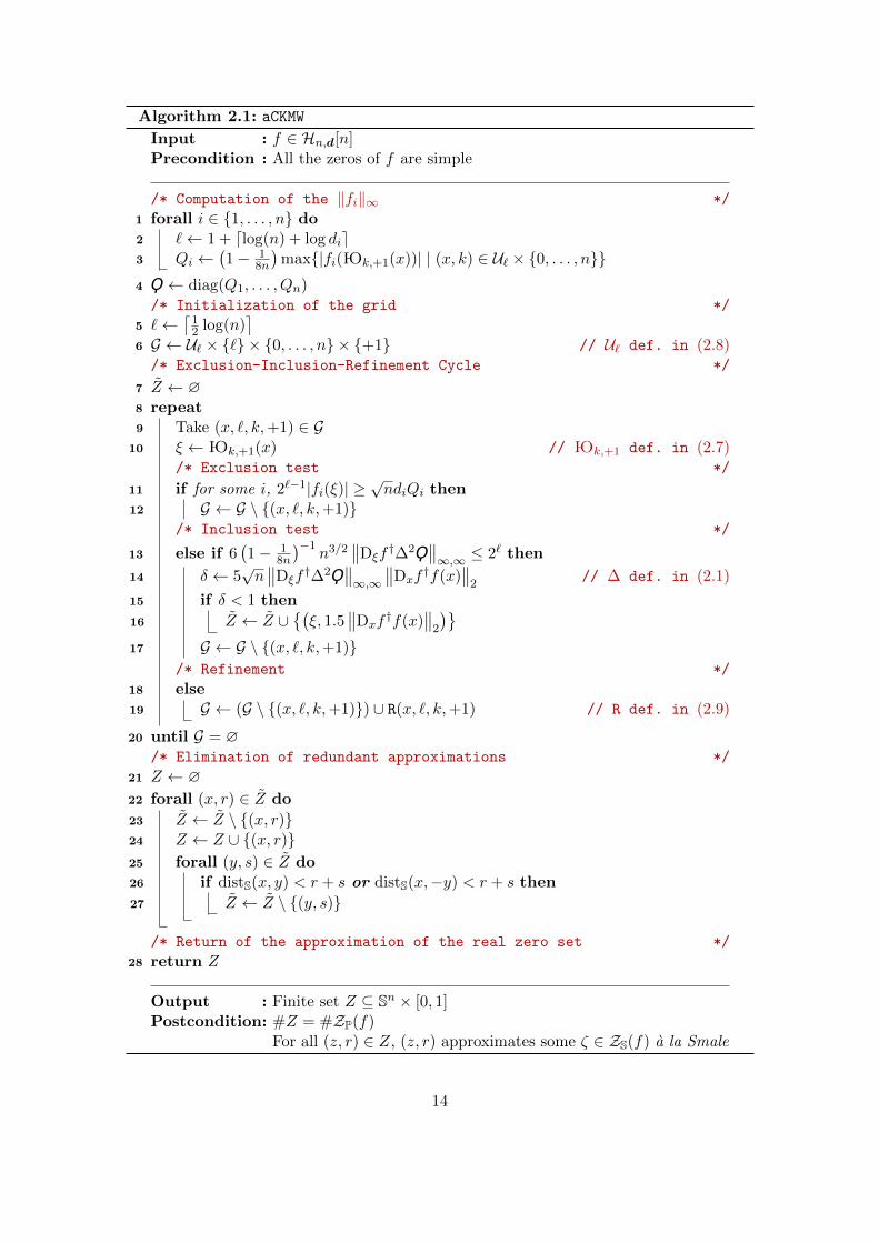
Algorithm 2.1: aCKMW
Input : f ∈ Hn,d[n]Precondition : All the zeros of f are simple
/* Computation of the ‖fi‖∞ */
1 forall i ∈ {1, . . . , n} do2 `← 1 + dlog(n) + log die3 Qi ←
(1− 1
8n
)max{|fi(�k,+1(x))| | (x, k) ∈ U` × {0, . . . , n}}
4 Ϙ← diag(Q1, . . . , Qn)/* Initialization of the grid */
5 `←⌈12 log(n)
⌉6 G ← U` × {`} × {0, . . . , n} × {+1} // U` def. in (2.8)/* Exclusion-Inclusion-Refinement Cycle */
7 Z ← ∅8 repeat9 Take (x, `, k,+1) ∈ G
10 ξ ←�k,+1(x) // �k,+1 def. in (2.7)/* Exclusion test */
11 if for some i, 2`−1|fi(ξ)| ≥√ndiQi then
12 G ← G \ {(x, `, k,+1)}/* Inclusion test */
13 else if 6(1− 1
8n
)−1n3/2
∥∥Dξf†∆2Ϙ
∥∥∞,∞ ≤ 2` then
14 δ ← 5√n∥∥Dξf
†∆2Ϙ∥∥∞,∞
∥∥Dxf†f(x)
∥∥2
// ∆ def. in (2.1)
15 if δ < 1 then
16 Z ← Z ∪{(ξ, 1.5
∥∥Dxf†f(x)
∥∥2
)}17 G ← G \ {(x, `, k,+1)}
/* Refinement */
18 else19 G ← (G \ {(x, `, k,+1)}) ∪ R(x, `, k,+1) // R def. in (2.9)
20 until G = ∅/* Elimination of redundant approximations */
21 Z ← ∅22 forall (x, r) ∈ Z do
23 Z ← Z \ {(x, r)}24 Z ← Z ∪ {(x, r)}25 forall (y, s) ∈ Z do26 if distS(x, y) < r + s or distS(x,−y) < r + s then
27 Z ← Z \ {(y, s)}
/* Return of the approximation of the real zero set */
28 return Z
Output : Finite set Z ⊆ Sn × [0, 1]Postcondition: #Z = #ZP(f)
For all (z, r) ∈ Z, (z, r) approximates some ζ ∈ ZS(f) a la Smale
14
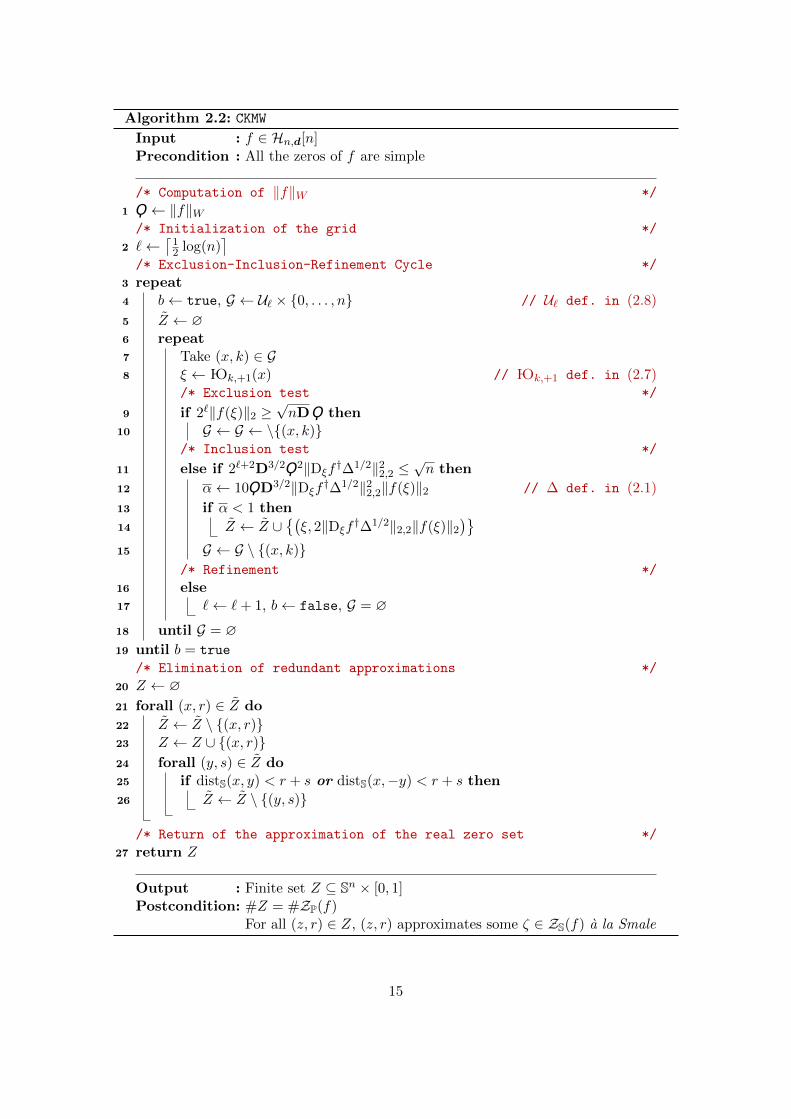
Algorithm 2.2: CKMW
Input : f ∈ Hn,d[n]Precondition : All the zeros of f are simple
/* Computation of ‖f‖W */
1 Ϙ← ‖f‖W/* Initialization of the grid */
2 `←⌈12 log(n)
⌉/* Exclusion-Inclusion-Refinement Cycle */
3 repeat4 b← true, G ← U` × {0, . . . , n} // U` def. in (2.8)
5 Z ← ∅6 repeat7 Take (x, k) ∈ G8 ξ ←�k,+1(x) // �k,+1 def. in (2.7)
/* Exclusion test */
9 if 2`‖f(ξ)‖2 ≥√nDϘ then
10 G ← G ← \{(x, k)}/* Inclusion test */
11 else if 2`+2D3/2Ϙ2‖Dξf†∆1/2‖22,2 ≤
√n then
12 α← 10ϘD3/2‖Dξf†∆1/2‖22,2‖f(ξ)‖2 // ∆ def. in (2.1)
13 if α < 1 then
14 Z ← Z ∪{(ξ, 2‖Dξf
†∆1/2‖2,2‖f(ξ)‖2)}
15 G ← G \ {(x, k)}/* Refinement */
16 else17 `← `+ 1, b← false, G = ∅
18 until G = ∅19 until b = true
/* Elimination of redundant approximations */
20 Z ← ∅21 forall (x, r) ∈ Z do
22 Z ← Z \ {(x, r)}23 Z ← Z ∪ {(x, r)}24 forall (y, s) ∈ Z do25 if distS(x, y) < r + s or distS(x,−y) < r + s then
26 Z ← Z \ {(y, s)}
/* Return of the approximation of the real zero set */
27 return Z
Output : Finite set Z ⊆ Sn × [0, 1]Postcondition: #Z = #ZP(f)
For all (z, r) ∈ Z, (z, r) approximates some ζ ∈ ZS(f) a la Smale
15
Note that the importance of approximations a la Smale is that they can be refined toany needed degree of precision fast. This is because, we can guarantee that the number ofbinary digits duplicates at each Newton iteration (quadratic convergence). Note that theδ-theorem (Theorem 2.10, provides a stronger convergence condition, but the given one isthe usual one.
We let the technical details of aCKMW to Section 4 where we will show that the algorithmis correct. Now, we give the intuition of the algorithm, so that one can see how all theingredients come together.
The algorithm is divided three main parts:
1. Computation of the norms
2. Cycle of Exclusion-Inclusion-Refinement
3. Elimination of redundant approximations
The computation of the norms is the most expensive part of the algorithm. While inCKMW, one only has to compute the Weyl norm; in aCKMW, we are required to compute theL∞-norms. This amounts to maximize a polynomial in the sphere, and it is the responsiblefor the Dn in the complexity estimates. As shown in [24, §3], the L∞-norms are neededfor obtaining the best complexity bounds for the grid method, despite the difficulty tocompute them.
In the cycle of Exclusion-Inclusion-Refinement, we do an exclusion test, an inclusiontest, if the latter fails; and we refine, if both tests fails. The main idea is to make the gridfiner and finer until we can certify at each point of the grid that either there are no rootsaround (exclusion) or that there is a root around (inclusion). For the exclusion test, weuse the exclusion lemma (Proposition 2.2); for the inclusion test, we use the δ-theorem(Theorem 2.10); and for the refinement we use the refinement operator R in (2.9).
In the above cycle, we can see several important difference between CKMW and aCKMW:
• Row-Normalization: We observe that while the normalization in CKMW is of the formf/‖f‖W , the normalization in aCKMW is the row-normalization defined in (2.2).
• Use of Smale’s β: Although aCKMW uses δ-theory instead of α-theory, this is notthe most important difference with CKMW. Note that δ-theory is nothing more thanα-theory adapted to homogeneous polynomials on the sphere. The main differenceis that aCKMW uses Smale’s β directly, without estimating it with expression of theform (1.4) and (2.5).
This difference between how β is used by both algorithm is the reason behind thedifferent form of the inequalities in line 13 of aCKMW and line 11 of CKMW. Theseconditions allow us to certify two things: 1) there is at most one root in BS(ξ,
√n2−`).
2) If there is such a root in BS(ξ,√n2−`) the inclusion test will be successful. Without
these two guarantees we risk undercounting the number of real roots.
• Local refinement : In CKMW, if any of the two tests fail, even if it just fails at a singlepoint, we refine the full grid. The latter means the lost of any information obtainedthrough the execution of the algorithm. In aCKMW, we avoid this lost of information,through means of local refinements. Of course, this is the adaptive character of thealgorithm.
16
In the elimination of redundant of redundant approximations, aCKMW and CKMW are verysimilar. The theoretical justification for the procedure in aCKMW is Proposition 2.13, whichguarantees that each approximation has only one zero in the ball considered around. Toavoid testing all possible pairs, we test one approximation against all other approximations,removing the ones that approximate the same root. Once we do this for one root, we don’thave to test the rest of the approximations against the removed roots.
Remark 2.17. We observe that instead of computing the ‖Dξf†∆2Ϙ‖∞,2 appearing in
the definition of ν(Ϙ−1f, ξ), we are computing the estimate ‖Dξf†∆2Ϙ‖∞,∞. The reason
for this is that while computing the first operator norm is computationally expensive,computing ‖Dξf
†∆2Ϙ‖∞,∞ is very cheap.
Remark 2.18. Note that we are not considering points (x, `, k, σ) only with σ = +1. Thisis because we are working in Pn and symmetry allows us to disregard half of the points tocheck.
Beyond the zero-dimensional case
If we are interested in the zero dimensional case, we can adapt turn aCKMW into Sampling
effortlessly. Unfortunately, there is no way of redundant approximations. Combining thepostcondition in Sampling with the results in [34, §2.3], where an adaptive version of theNiyogi-Smale-Weinberger theorem is proven following on work of [45, 44], we can guaranteetopological correctness. By this, we mean that we can guarantee that the inclusion ZS(f) ⊂⋃{BP(z, r) | (z, r) ∈ Z or (−z, r) ∈ Z} is an homotopy equivalence. Unfortunately, we are
unaware of any way of exploiting this to obtain an algorithm that computes the homologyor Betti numbers of smooth projective algebraic sets in finite expected time. We hope toexplore this possibility, the main motivation of this paper, in future work.
The condition-based complexity analysis of Sampling is almost identical to that ofaCKMW and we omit it. The probabilistic complexity analysis is harder than that of aCKMWbut it can be done using similar techniques to the ones we use in this paper. However,we omit such proofs, as we plan to include probabilistic complexity analyses under moregeneral hypotheses in future work.
2.3 Complexity results
In Section 4, we will perform a condition-based complexity of our algorithms in terms of
Ex∈SnC(f, x)n logl C(f, x),
where C was given in Definition 2.7. In these estimates l will vary depending on whetherwe only count arithmetic operations (the main case that we will consider in Section 4) orif we count bit operations (up to some degree) of the finite precision version (discussed inSection 5).
Now, condition-based complexity bounds explain why and how a numerical algorithmis faster depending on the input. Unfortunately, these input-dependent estimates do notgive a good idea about the complexity of an algorithm. A long tradition in numerical com-plexity, going back to Goldstine and von Neumann [42] and popularized by Demmel [32]and Smale [73, 72], is to randomize the input and consider the probabilistic behaviour ofthe algorithm. In this way, when we talk about expected run-time, we do so with respecta distribution or family of distributions of the input space.
17
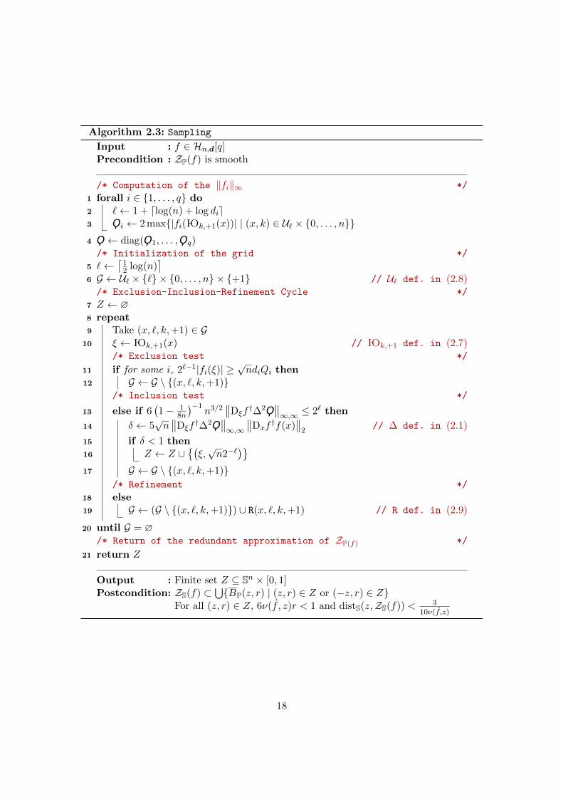
Algorithm 2.3: Sampling
Input : f ∈ Hn,d[q]Precondition : ZP(f) is smooth
/* Computation of the ‖fi‖∞ */
1 forall i ∈ {1, . . . , q} do2 `← 1 + dlog(n) + log die3 Ϙi ← 2 max{|fi(�k,+1(x))| | (x, k) ∈ U` × {0, . . . , n}}4 Ϙ← diag(Ϙ1, . . . ,Ϙq)/* Initialization of the grid */
5 `←⌈12 log(n)
⌉6 G ← U` × {`} × {0, . . . , n} × {+1} // U` def. in (2.8)/* Exclusion-Inclusion-Refinement Cycle */
7 Z ← ∅8 repeat9 Take (x, `, k,+1) ∈ G
10 ξ ←�k,+1(x) // �k,+1 def. in (2.7)/* Exclusion test */
11 if for some i, 2`−1|fi(ξ)| ≥√ndiQi then
12 G ← G \ {(x, `, k,+1)}/* Inclusion test */
13 else if 6(1− 1
8n
)−1n3/2
∥∥Dξf†∆2Ϙ
∥∥∞,∞ ≤ 2` then
14 δ ← 5√n∥∥Dξf
†∆2Ϙ∥∥∞,∞
∥∥Dxf†f(x)
∥∥2
// ∆ def. in (2.1)
15 if δ < 1 then16 Z ← Z ∪
{(ξ,√n2−`
)}17 G ← G \ {(x, `, k,+1)}
/* Refinement */
18 else19 G ← (G \ {(x, `, k,+1)}) ∪ R(x, `, k,+1) // R def. in (2.9)
20 until G = ∅/* Return of the redundant approximation of ZP(f) */
21 return Z
Output : Finite set Z ⊆ Sn × [0, 1]Postcondition: ZS(f) ⊂
⋃{BP(z, r) | (z, r) ∈ Z or (−z, r) ∈ Z}
For all (z, r) ∈ Z, 6ν(f , z)r < 1 and distS(z,ZS(f)) < 310ν(f ,z)
18
As it usual for numerical algorithms, these kind of condition-based complexity es-timates are not illustrative of the average behaviour of the algorithm. Following , werandomize the input of the algorithm to be able to talk about the expected run-time,which should give an idea of how the algorithm could work in practice. Moreover, we willconsider also an smoothed analysis of our algorithm.
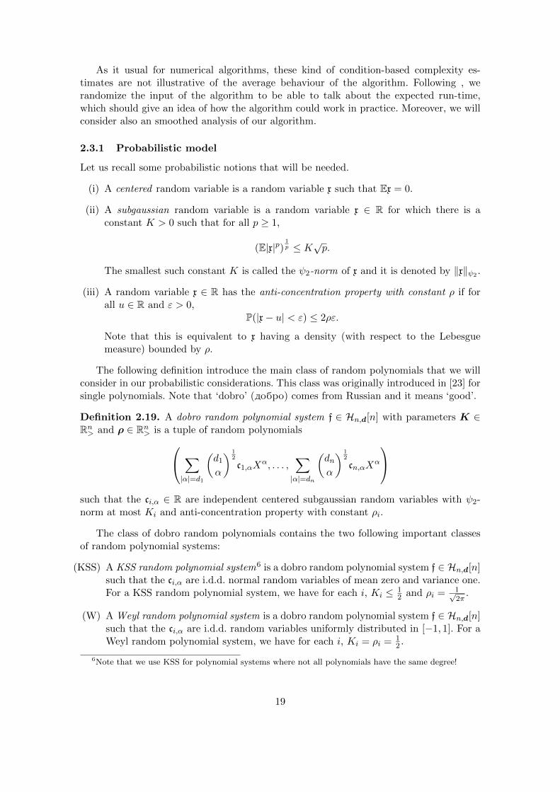
2.3.1 Probabilistic model
Let us recall some probabilistic notions that will be needed.
(i) A centered random variable is a random variable x such that Ex = 0.
(ii) A subgaussian random variable is a random variable x ∈ R for which there is aconstant K > 0 such that for all p ≥ 1,
(E|x|p)1p ≤ K√p.
The smallest such constant K is called the ψ2-norm of x and it is denoted by ‖x‖ψ2 .
(iii) A random variable x ∈ R has the anti-concentration property with constant ρ if forall u ∈ R and ε > 0,
P(|x− u| < ε) ≤ 2ρε.
Note that this is equivalent to x having a density (with respect to the Lebesguemeasure) bounded by ρ.
The following definition introduce the main class of random polynomials that we willconsider in our probabilistic considerations. This class was originally introduced in [23] forsingle polynomials. Note that ‘dobro’ (dobro) comes from Russian and it means ‘good’.
Definition 2.19. A dobro random polynomial system f ∈ Hn,d[n] with parameters K ∈Rn> and ρ ∈ Rn> is a tuple of random polynomials ∑
|α|=d1
(d1α
) 12
c1,αXα, . . . ,
∑|α|=dn
(dnα
) 12
cn,αXα
such that the ci,α ∈ R are independent centered subgaussian random variables with ψ2-norm at most Ki and anti-concentration property with constant ρi.
The class of dobro random polynomials contains the two following important classesof random polynomial systems:
(KSS) A KSS random polynomial system6 is a dobro random polynomial system f ∈ Hn,d[n]such that the ci,α are i.d.d. normal random variables of mean zero and variance one.For a KSS random polynomial system, we have for each i, Ki ≤ 1
2 and ρi = 1√2π
.
(W) A Weyl random polynomial system is a dobro random polynomial system f ∈ Hn,d[n]such that the ci,α are i.d.d. random variables uniformly distributed in [−1, 1]. For aWeyl random polynomial system, we have for each i, Ki = ρi = 1
2 .
6Note that we use KSS for polynomial systems where not all polynomials have the same degree!
19
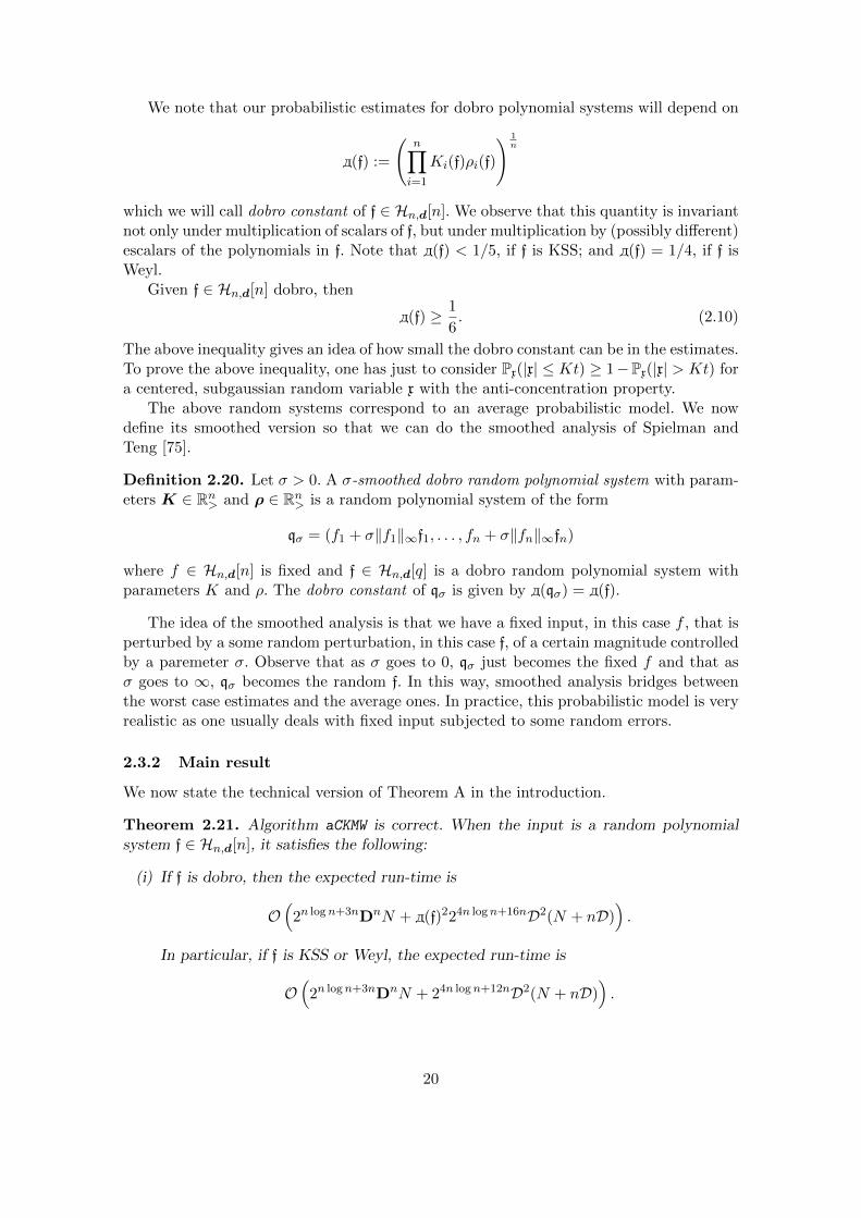
We note that our probabilistic estimates for dobro polynomial systems will depend on
d(f) :=
(n∏i=1
Ki(f)ρi(f)
) 1n
which we will call dobro constant of f ∈ Hn,d[n]. We observe that this quantity is invariantnot only under multiplication of scalars of f, but under multiplication by (possibly different)escalars of the polynomials in f. Note that d(f) < 1/5, if f is KSS; and d(f) = 1/4, if f isWeyl.
Given f ∈ Hn,d[n] dobro, then
d(f) ≥ 1
6. (2.10)
The above inequality gives an idea of how small the dobro constant can be in the estimates.To prove the above inequality, one has just to consider Px(|x| ≤ Kt) ≥ 1−Px(|x| > Kt) fora centered, subgaussian random variable x with the anti-concentration property.
The above random systems correspond to an average probabilistic model. We nowdefine its smoothed version so that we can do the smoothed analysis of Spielman andTeng [75].
Definition 2.20. Let σ > 0. A σ-smoothed dobro random polynomial system with param-eters K ∈ Rn> and ρ ∈ Rn> is a random polynomial system of the form
qσ = (f1 + σ‖f1‖∞f1, . . . , fn + σ‖fn‖∞fn)
where f ∈ Hn,d[n] is fixed and f ∈ Hn,d[q] is a dobro random polynomial system withparameters K and ρ. The dobro constant of qσ is given by d(qσ) = d(f).
The idea of the smoothed analysis is that we have a fixed input, in this case f , that isperturbed by a some random perturbation, in this case f, of a certain magnitude controlledby a paremeter σ. Observe that as σ goes to 0, qσ just becomes the fixed f and that asσ goes to ∞, qσ becomes the random f. In this way, smoothed analysis bridges betweenthe worst case estimates and the average ones. In practice, this probabilistic model is veryrealistic as one usually deals with fixed input subjected to some random errors.
2.3.2 Main result
We now state the technical version of Theorem A in the introduction.
Theorem 2.21. Algorithm aCKMW is correct. When the input is a random polynomialsystem f ∈ Hn,d[n], it satisfies the following:
(i) If f is dobro, then the expected run-time is
O(
2n logn+3nDnN + d(f)224n logn+16nD2(N + nD)).
In particular, if f is KSS or Weyl, the expected run-time is
O(
2n logn+3nDnN + 24n logn+12nD2(N + nD)).
20
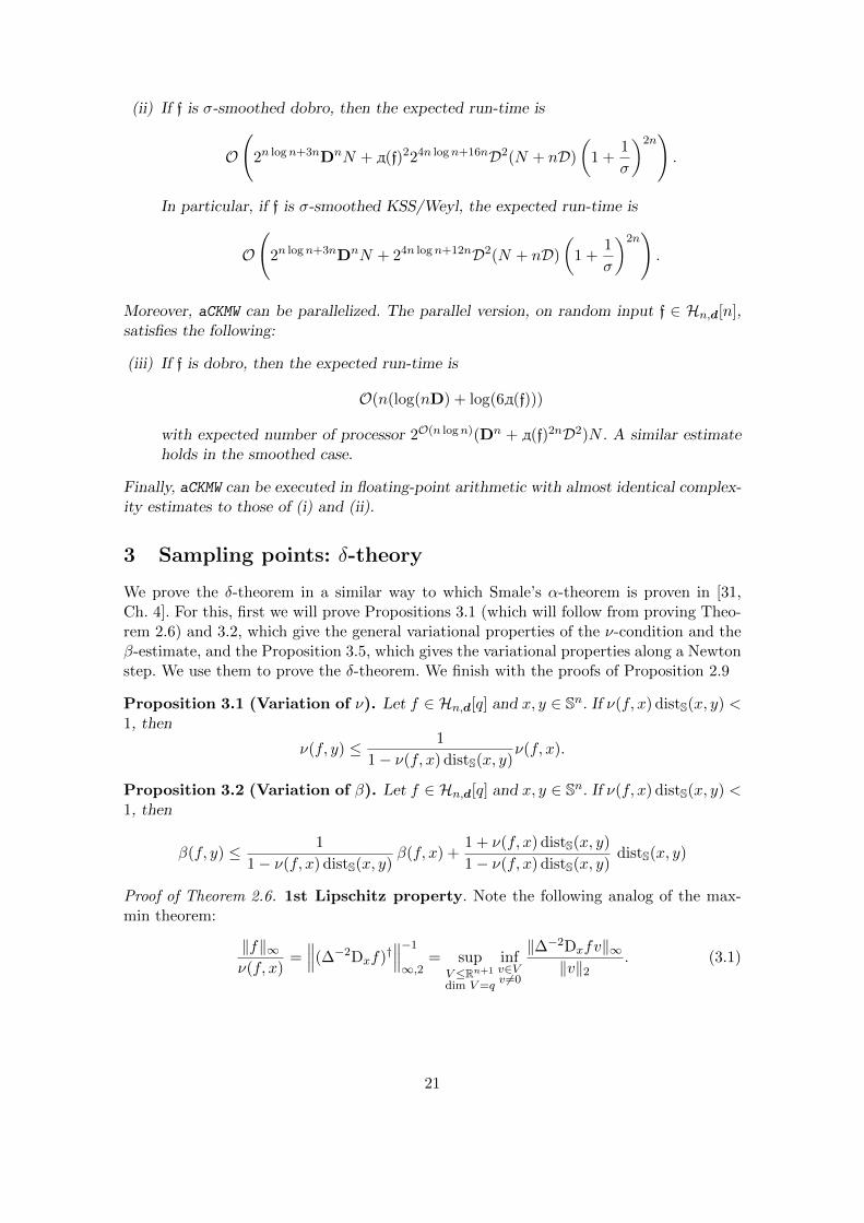
(ii) If f is σ-smoothed dobro, then the expected run-time is
O
(2n logn+3nDnN + d(f)224n logn+16nD2(N + nD)
(1 +
1
σ
)2n).
In particular, if f is σ-smoothed KSS/Weyl, the expected run-time is
O
(2n logn+3nDnN + 24n logn+12nD2(N + nD)
(1 +
1
σ
)2n).
Moreover, aCKMW can be parallelized. The parallel version, on random input f ∈ Hn,d[n],satisfies the following:
(iii) If f is dobro, then the expected run-time is
O(n(log(nD) + log(6d(f)))
with expected number of processor 2O(n logn)(Dn + d(f)2nD2)N . A similar estimateholds in the smoothed case.
Finally, aCKMW can be executed in floating-point arithmetic with almost identical complex-ity estimates to those of (i) and (ii).
3 Sampling points: δ-theory
We prove the δ-theorem in a similar way to which Smale’s α-theorem is proven in [31,Ch. 4]. For this, first we will prove Propositions 3.1 (which will follow from proving Theo-rem 2.6) and 3.2, which give the general variational properties of the ν-condition and theβ-estimate, and the Proposition 3.5, which gives the variational properties along a Newtonstep. We use them to prove the δ-theorem. We finish with the proofs of Proposition 2.9
Proposition 3.1 (Variation of ν). Let f ∈ Hn,d[q] and x, y ∈ Sn. If ν(f, x) distS(x, y) <1, then
ν(f, y) ≤ 1
1− ν(f, x) distS(x, y)ν(f, x).
Proposition 3.2 (Variation of β). Let f ∈ Hn,d[q] and x, y ∈ Sn. If ν(f, x) distS(x, y) <1, then
β(f, y) ≤ 1
1− ν(f, x) distS(x, y)β(f, x) +
1 + ν(f, x) distS(x, y)
1− ν(f, x) distS(x, y)distS(x, y)
Proof of Theorem 2.6. 1st Lipschitz property. Note the following analog of the max-min theorem:
‖f‖∞ν(f, x)
=∥∥∥(∆−2Dxf)†
∥∥∥−1∞,2
= supV≤Rn+1
dim V=q
infv∈Vv 6=0
‖∆−2Dxfv‖∞‖v‖2
. (3.1)
21
If Dxf is not surjective, then both sizes are zero and the equality holds. If Dxf is surjective,then∥∥∥(∆−2Dxf)†
∥∥∥−1∞,2
= infw 6=0
‖w‖∞‖(∆−2Dxf)†w‖2
= infv∈kerDxf⊥
v 6=0
‖∆−2Dxfv‖∞‖(∆−2Dxf)†∆−2Dxfv‖2
= infv∈(kerDxf)⊥
v 6=0
‖∆−2Dxfv‖∞‖v‖2
,
giving that the left-hand side is bounded by the right-hand side. For the other inequality,take a subspace V of Rn+1 of dimension q such that V ∩ker Dxf = 0, so that the orthogonalprojection P : V → (ker Dxf)⊥ is injective. Otherwise, the infimum on the right hand sidewould be zero. Then
infv∈Vv 6=0
‖∆−2Dxfv‖∞‖v‖2
≤ infv∈Vv 6=0
‖∆−2Dxfv‖∞‖Pv‖2
= infv∈Vv 6=0
‖∆−2Dxf(Pv)‖∞‖Pv‖2
= infv∈(kerDxf)⊥
v 6=0
‖∆−2Dxfv‖∞‖v‖2
=∥∥∥(∆−2Dxf)†
∥∥∥∞,2
,
where we use that projecting in the orthogonal complement of the kernel does not alterthe image. Thus the wanted equality follows.
Using the above max-min theorem and that taking maximums and minimums preservesLipschitz properties, we have that∣∣∣∣ ‖g‖∞ν(g, x)
− ‖g‖∞ν(g, x)
∣∣∣∣ ≤ ‖∆−2Dx(g − g)‖2,∞.
Now, by Kellogg’s theorem (Theorem 2.1),
‖∆−2Dxh‖2,∞ ≤ maxi
supv 6=0
1
d2i
|∂xhiv|‖v‖2
≤ maxi
‖hi‖∞di
= ‖∆−1h‖∞, (3.2)
so the 1st Lipschitz inequality follows. For the other inequality, take in the 1st Lipschitzinequality, g = f and g = 0, so that
ν(f, x) ≥ ‖f‖∞‖∆−1f‖∞
≥ 1.
2nd Lipschitz property. Let y, y ∈ Sn and u ∈ O(n + 1) be the planar rotationsending x to y. Then∣∣∣∣ 1
ν(f, y)− 1
ν(f, y)
∣∣∣∣ =1
‖f‖∞
∣∣∣∣ ‖fu‖∞ν(fu, y)− ‖f‖∞ν(f, y)
∣∣∣∣where fu := f(uX), by the chain rule and the invariance of the L∞-norm. Thus, by the1st Lipschitz property, ∣∣∣∣ 1
ν(f, y)− 1
ν(f, y)
∣∣∣∣ ≤ ‖∆−1(fu − f)‖∞‖f‖∞
.
Now, ‖∆−1(fu − f)‖∞ = maxz∈Sn ‖∆−1f(uz)−∆−1f(z)‖∞. By Kellogg’s theorem (The-orem 2.1), ∆−1f is ‖f‖∞-Lipschitz, since each d−1i fi is ‖fi‖∞-Lipschitz. Thus
‖∆−1f(uz)−∆−1f(z)‖∞ ≤ ‖f‖∞ distS(z, uz) ≤ ‖f‖∞ distS(y, y)
where the last inequality follows because u is the planar rotation taking y to y.
22
Proof of Proposition 3.1. By the 2nd Lipschitz property of the ν-condition (Theorem 2.6),x 7→ 1/ν(f, x) is 1-Lipschitz (with respect the geodesic distance on Sn). The propositionis just a rewriting of this condition.
Lemma 3.3. Let f ∈ Hn,d[q] and x, y ∈ Sn. Then
‖Dyf†Dxf‖2,2 ≤
1
1− ν(f, x) distS(x, y).
Lemma 3.4. Let f ∈ Hn,d[q] and x, y ∈ Sn be such that y 6= −x. Then
‖Dxf†f(y)‖2 ≤
∥∥∥Dxf†f(x) + distS(x, y)Dxf
†Dxfυx,y
∥∥∥2
+1
2ν(f, x) distS(x, y)2
where υx,y := (y − 〈y, x〉x)/ sin distS(x, y) is the tangent unit vector at x of the geodesicjoining x to y.
Proof of Proposition 3.2. Note that
β(f, y) = ‖Dyf†DxfDxf
†f(y)‖2 ≤ ‖Dyf†Dxf‖2,2‖Dxf
†f(y)‖2,
since DxfDxf† = I. The propositions follows now from Lemmas 3.3 and 3.4, 1/2 ≤ 1, the
triangle inequality and that Dxf†Dxf is an orthogonal projection.
Proof of Lemma 3.3. Note that for f, g ∈ Hn,d[q] and z ∈ Sn,
‖Dzg†Dzf‖2,2 ≤ ‖Dzg
†Dzg‖2,2 + ‖Dzg†Dz(f − g)‖2,2
≤ 1 + ‖Dzg†Dz(f − g)‖2,2
(Dzg
†Dzg is an orthogonal projection)
≤ 1 + ν(g, z)‖∆−2Dz(f − g)‖2,∞
‖g‖∞(Definition of ν-condition)
≤ 1 + ν(g, z)‖∆−1(f − g)‖∞
‖g‖∞. (Kellogg’s theorem, applied as in (3.2))
Now, let u ∈ O(n+ 1) be the planar rotation taking x to y. Then
‖Dyf†Dxf‖ = ‖Dx(fu)†Dxf‖.
Hence, arguing as in the proof of the 2nd Lipschitz property, but using the inequalityabove, we get
‖Dyf†Dxf‖ ≤ 1 + ν(f, y) distS(x, y).
Finally, Proposition 3.1 finishes the proof.
Proof of Lemma 3.4. For any smooth path ϑ : [0, 1]→ Rn+1, we have by Taylor’s theoremthat
‖ϑ(1)‖2 ≤ ‖ϑ(0) + ϑ′(0)‖2 +1
2maxs∈[0,1]
‖ϑ′′(s)‖2.
Now, let [0, 1] 3 t 7→ xt ∈ Sn a constant speed geodesic joining x and y and ϑ : [0, 1] →Rn+1 the smooth path given by ϑ(t) = Dxf
†f(xt). By the chain rule,
ϑ′(0) = distS(x, y)Dxf†Dxfυx,y = distS(x, y)υx,y,
23
since ∂xfυx,y = Dxfυx,y since x ∈ ker Dxf and υx,y is orthogonal to x; and
ϑ′′(s) = Dxf† (∂2xsf (xs, xs)−∆f(xs) distS(x, y)2
),
since xs = −distS(x, y)2xs and Dxf(xt) = ∆f(xt) by Euler’s formula for homogeneouspolynomials.
Now,
‖ϑ′′(s)‖2 ≤ ν(f, x)1
‖f‖∞∥∥∆−2∂2xsf (xs, xs)−∆−1f(xs) distS(x, y)2
∥∥∞ .
Now, by the triangle inequality, the above is bounded by
maxi
(|d−2i ∂2xsf (xs, xs) |+ |d−1i f(xs)|distS(x, y)2
).
Applying Kellogg’s inequality (Theorem 2.1, we get that
|d−2i ∂2xsf (xs, xs) | ≤(
1− 1
di
)‖f‖∞ distS(x, y)2 and |d−1i f(xs)| ≤
1
di‖f‖∞,
since ‖xs‖2 = distS(x, y). Hence
1
2maxs∈[0,1]
‖ϑ′′(s)‖2 ≤1
2
and the result follows.
Proposition 3.5 (Variation along a Newton step). Let f ∈ Hn,d[q] and x ∈ Sn besuch that δ(f, x) < 1. Then N2
f (x) is defined,
β(f,Nf (x)) ≤ 1
2
1 + δ(f, x)
1− δ(f, x)δ(f, x)β(f, x)
and
δ(f,Nf (x)) ≤ 1
2
1 + δ(f, x)
(1− δ(f, x))2δ(f, x)2.
Proof. We note that N2f (x) is well-defined, since DNf (x)f is surjective as ν(f,N(f, x)) <∞
by Proposition 3.1 and ν(f, x) distS(x,Nf (x)) ≤ δ(f, x) < 1.For the bound on β(f,Nf (x)), we argue as in Proposition 3.2 using Lemmas 3.3 and 3.4.
The main trick is that when we apply Lemma 3.4, we get that∥∥∥Dxf†f(x)− distS(x,Nf (x))DxfDxf
†υx,Nf (x)
∥∥∥ = β(f, x)|β(f, x)− arctanβ(f, x)|
≤ 1
3β(f, x)3
due to υx,Nf (x) = −Dxf†f(x)/β(f, x), (2.3) and (2.4). Hence
β(f,Nf (x)) ≤12 + 1
3β(f, x)
1− δ(f, x)δ(f, x)β(f, x).
The desired bound for β(f,Nf (x)) follows after noting that
1
2+
1
3β(f, x) ≤ 1
2+
1
3δ(f, x) ≤ 1
2(1 + δ(f, x)),
since ν(f, x) ≥ 1 by the 1st Lipschitz property (Theorem 2.6). For the inequality regardingδ(f,Nf (x)), we combined the inequality for β obtained with the one in Proposition 3.1.
24
Proof of the δ-Theorem (Theorem 2.10). We will show by induction that the Newton se-quence is well-defined and that
δ(f,Nkf (x)) ≤
(1
3
)2k−1δ(f, x)
and
β(f,Nkf (x)) ≤
(3
4
)k (1
3
)2k−1β(f, x)
using Proposition 3.5.Clearly both claims are true for k = 0, so the base case is true. We now show the
induction step. By Proposition 3.5 and the induction hypothesis, Nk+1f (x) = Nf (Nk
f (x)) iswell-defined,
β(f,Nk+1f (x)) ≤ 1
2
1 + δ(f,Nkf (x))
1− δ(f,Nkf (x))
δ(f,Nkf (x))β(f,Nk
f (x))
≤ 1
2
1 + δ(f, x)
1− δ(f, x)δ(f, x)
(3
4
)k (1
3
)2k+1−2β(f, x)
and
δ(f,Nk+1f (x)) ≤ 1
2
1 + δ(f,Nkf (x))
(1− δ(f,Nkf (x)))2
δ(f,Nkf (x))2
≤ 1
2
1 + δ(f, x)
(1− δ(f, x))2δ(f, x)
(1
3
)2k+1−2δ(f, x),
where we have used that both
t 7→ 1
2
1 + t
1− tand t 7→ 1
2
1 + t
(1− t)2
are monotonous on t for t ∈ [0, 1] and that β(f,Nkf (x)) ≤ β(f, x) and δ(f,Nf (x)) ≤ δ(f, x).
Now, by assumption, δ(f, x) ≤ 1/4, so
1
2
1 + δ(f, x)
(1− δ(f, x))δ(f, x) <
1
4and
1
2
1 + δ(f, x)
(1− δ(f, x))2δ(f, x) <
1
3. (3.3)
Hence our inductive claims hold. This shows 1 and 2.For 3, we note that for all k >= 0,
distS
(Nkf (x),Nk+1
f (x))≤(
3
4
)k (1
3
)2k−1β(f, x) ≤ 1
4
(3
4
)k (1
3
)2k−1 1
ν(f, x).
Adding the sum, the desired claim follows.
Remark 3.6. In the above proof, we can see that to improve the constants in the δ-theorem, we can just play we the values of δ(f, x) and the bounds obtained in (3.3). Forgetting quadratic convergence, we can use δ(f, x) < 1/3; and for getting convergence,
δ(f, x) ≤ 5−√17
2 ≈ 0.4385 . . .
We now prove the converses to the α-theorem and to the δ-theorem.
25
Proof of Proposition 2.9. Let ζ ∈ ZS be the nearest zero to x. Then, by Taylor’s theorem,
−Dxf†f(x) = Dxf
†f(ζ)−Dxf†f(x) =
∞∑k=1
1
k!Dxf
†∂kx(ζ − x, . . . , ζ − x).
Now, taking norms,
β(f, x) = ‖Dxf†Dxf(ζ − x)‖2 +
∞∑k=2
∥∥∥∥ 1
k!Dxf
†∂kx(ζ − x, . . . , ζ − x)
∥∥∥∥2
.
where the first summand side is bounded by ‖ζ − x‖2, since Dxf†Dxf is an orthogonal
projection, and the kth summand in the series is bounded by γ(f, x)k−1‖ζ − x‖k2. Hence,we have that,
β(f, x) ≤ distS(x,ZS(f))
( ∞∑k=0
(γ(f, x) distS(x,ZS(f)))k)
=distS(x,ZS(f))
1− γ(f, x) distS(x,ZS(f))
The rest follows from the Higher Derivative Estimate (2.6).
Proof of Theorem 2.11. We argue as in Lemma 3.4, taking the same map ϑ, but withy ∈ ZS(f) the nearest point to x. Using Taylor’s theorem for a smooth map ϑ : [0, 1]→ Sn,we have that
‖ϑ(1)− ϑ(0)‖2 ≤ ‖ϑ′(0)‖2 +1
2maxs∈[0,1]
‖ϑ′′(s)‖2.
Taking ϑ as in the proof of Lemma 3.4, , and arguing analogously, we obtain that
β(f, x) ≤ distS(x,ZS(f)) +1
2ν(f, x) distS(x,ZS(f))2.
Multiplying by ν(f, x) gives the desired bound.
We finish the section with the proof of Proposition 2.13.
Proof of Proposition 2.13. The proof follows a similar idea to the proof in of [1, p. 161],but with he technical difficulties associated to working in the sphere. Without loss ofgenerality, we assume that ‖f‖∞ = 1.
Let ζ0, ζ1 ∈ BS(x, 1/(3ν(f, x))) be distinct zeros of f . Let [0, 1] 3 t 7→ ζt be the constantspeed geodesic joining them. For each i, we have that t 7→ fi(ζt) takes the value 0 at theextremes of [0, 1]. Therefore, by Rolle’s theorem, for each i, there is some ti so that
Dζtifi(ζti) = 0.
Let y = ζ1/2 be the point equidistant to ζ0 and ζ1 in the geodesic joining them, and
v = ζ1/2 the tangent vector of the considered constant speed geodesic. Let u1, . . . , un bethe planar rotations that send y respectively to ζt1 , . . . , ζtn . These planar rotations can beobtained by rotating the plane containing ζ0, ζ1 and the geodesic joining them. Note that,because of this, we must have that
uiv = ζti ,
since these rotations must preserve tangent vectors along the geodesic joining ζ0 and ζi.
26
Let g = (fuii ). By assumption and orthogonal invariance, ‖g‖∞ = ‖f‖∞ = 1. Byconstruction, Dyg : TySn → Rn is not surjective, since v ∈ ker Dyg. Note that here it isessential that g is an n-tuple and not a q-tuple. Therefore
ν(g, y) =∞.
Now, we show that the above equality cannot happen. Therefore we cannot have tworoots inside the considered ball. By the Lipschitz properties in Theorem 2.6,
1
ν(g, y)≥ 1
ν(g, x)− distS(x, y) (2nd Lipschitz prop. of ν)
≥ 1
ν(f, x)−∥∥∆−1(g − f)
∥∥∞ − distS(x, y) (1st Lipschitz prop. of ν)
≥ 1
ν(f, x)−max
i
∥∥d−1i (fuii − fi)∥∥∞ − distS(x, y)
≥ 1
ν(f, x)−max
imaxz∈Sn
dist(z, uiz)− distS(x, y) (Kellogg’s Theorem (2.1)).
As ui is the planar rotation taking y = ζ1/2 to ζti along the geodesic where they lie, wehave that
dist(z, uiz) ≤ distS(ζ1/2, ζti) ≤1
2distS(ζ0, ζ1).
Hence1
ν(g, y)≥ 1
2ν(f, x),
since y, ζ0, ζ1 ∈ BS(x, 1/(3ν(f, x))). But this means that
ν(g, y) ≤ 2ν(f, x) <∞,
obtaining the desired contradiction.
4 Complexity Analysis
We now give the complexity analysis, which is the core of this paper. First, we give severalcondition-based complexity analyses; then we use them to produce probabilistic complexityanalyses.
4.1 Condition-based complexity analysis
The following theorem gives the condition-based estimate from where all our probabilisticestimates will be deduced.
Theorem 4.1. Algorithm aCKMW is correct. When the input is a polynomial system f ∈Hn,d[n], its run-time is bounded by
O
2n logn+3nDnN + voln(Sn)
(3n
2
)n(N + nD)
Ex∈Sn
C(f , x)n
‖x‖n+1∞
.
27
Remark 4.2. We note that
voln(Sn)Ex∈Sn1
‖x‖n+1∞
= 2n(n+ 1), (4.1)
due to the change of variables formula. Because of this, we don’t estimate further theelements in the statement above.
Recall that in both algorithms we are just bounding the number of arithmetic opera-tions. We divide the analysis between the three main part of aCKMW: 1) computation of thenorms, 2) the Exclusion-Inclusion-Refinement Cycle, and 3) the elimination of redundantapproximations. The proof of Theorem 4.1 follows from combining Propositions 4.3, 4.5and 4.6.
4.1.1 Computation of the norms (Lines 1-3)
To compute the L∞-norms, the main result is [24, Proposition 4.2].
Proposition 4.3. Let f ∈ Hn,d be an homogeneous polynomial of degree d and G ⊂ Snsuch that for every x ∈ Sn, distS(x,G) ≤ η. If dη ≤ 1, then
maxx∈G‖f(x)‖∞ ≤ ‖f‖∞ ≤
1
1− D2
2 η2
maxx∈G‖f(x)‖∞.
Using the above proposition, one proves the following result in a similar way to [24,Proposition 4.4].
Proposition 4.4. In lines 7-3 of aCKMW, the computed Qi satisfy that(1− 1
8n
)Qi ≤ ‖fi‖∞ ≤ Qi.
Moreover, this computation requires
O(
2n logn+3nDnN)
arithmetic operations.
Proof. We note that |U`| = 2`n. In this way, for each fi, we do O(n2nd1+logn+log die
)evalu-
ations, taking each one of them O((
n+din
))arithmetic operations (see [12, Lemma 16.31]).
The property of the Qi is justified by Proposition 4.3, since, by construction, for all i andall x ∈ Sn, distS(x,�k,+1(U`)) ≤ 1/di.
4.1.2 Exclusion-Inclusion-Refinement Cycle (Lines 7-20)
The next proposition is reminiscent of the continuous amortization of Burr, Krahmer andYap [17].
Proposition 4.5. Lines 7-20 of aCKMW satisfy the following:
28
(a) If for all i, ‖fi‖∞ ≤ Qi, then, at the end of the execution, we have that for all(z, r) ∈ Z, BS(z, r) contains exactly one root of f , of which (z, r) is an approximationa la Smale. And reciprocally, for each ζ ∈ ZS(f), there is some (z, r) ∈ Z such thatζ ∈ BS(z, r) ∪BS(−z, r).
(b) The total number of points that were processed in the cycle is bounded by
(3n
2
)n ∫x∈Sn
C(f , x
)n‖x‖n+1
∞dx.
(c) The total number of arithmetic operations is bounded by
O
(3n
2
)nN
∫x∈Sn
C(f , x
)n‖x‖n+1
∞dx
.
Proof of Proposition 2.15. (i) This is by construction.(ii) The refinement operator substitutes a cube by 2n copies of cube with half the
width. Therefore it preserves the cubical grid property.(iii) This follows from the fact that the �k,σ are 1-Lipschitz with the Euclidean dis-
tance in the domain and the geodesic distance in the codomain. Note that the√n comes
from the relation between the ∞-norm and the Euclidean norm.
Proof of Proposition 4.5. (a) Notice that(1− 1
8n
)‖∆−1f(ξ)‖∞ ≤ ‖Ϙ−1∆−1f(ξ)‖∞ ≤ ‖∆−1f(ξ)‖∞ (4.2)
and that1√nν(f , x) ≤ ‖Dξf
†∆2Ϙ‖∞,∞ ≤(
1− 1
8n
)−1ν(f , x) (4.3)
since for all i,(1− 1
8n
)≤ ‖fi‖∞/Ϙi ≤ 1.
If the inequality in line 11 holds, then
‖Ϙ−1∆−1f(ξ)‖∞ ≥√n21−`,
and so, by (4.2),‖∆−1f(ξ)‖∞ ≥
√n21−`.
Hence the exclusion lemma (Proposition 2.2) guarantees that there are not any roots insideBS(ξ,
√n21−`), so the exclusion is justified.
If the inequality in line 13 is satisfied, then, by (4.3),
6
(1− 1
8n
)−1nν(f , ξ) ≤ 2`
and so
BS(ξ,√n2−`) ⊆ BS
(ξ,
(1− 1
8n
)1
6√nν(f , ξ)
).
29
By the converse of the δ-theorem (Proposition 2.11), if there is a root ζ of f inBS(ξ,√n2−`),
then
5
(1− 1
8n
)−1√nδ(f , x) < 1,
and so, by (4.3),5√n‖Dξf
†∆2Ϙ‖∞,∞‖Dξf†f(ξ)‖2 ≤ 1.
Thus we conclude that the inclusion test would be passed in this case. Note that byconstruction of the adaptive grid (Proposition 2.15), the above situation happens to everypossible projective root.
Now, if the inclusion test is passed, this means that, by (4.3), the hypothesis of the δ-theorem (Theorem 2.10) holds, and so there is a root ζ ∈ ZS(f) such that (ξ, 1.5‖Dξf
†f(ξ)‖2)is an approximation a la Smaleof ζ, and such that
distS(ξ, ζ) ≤ 1.5‖Dξf†f(ξ)‖2 ≤
3
10
1
ν(f , x)<
1
3ν(f , x).
Hence ζ is the unique root of f in BS
(ξ, 1
3ν(f ,ξ)
), by Proposition 2.13. Note that this
means that if there was a root in and such that . This justifies the inclusion of the point.
Moreover, note that if there was a root in BS(ξ,√n2−`) ⊂ BS
(ξ, 1
3ν(f ,ξ)
), it has to be ζ.
Thus (a) follows, as this happens to every root.(b) Let (x, `, k,+1) ∈ G be a point that either passes either the test in line 11 or the test
in line 13, and (y, `−1, k,+1) the parent of (x, `, k,+1), i.e., (x, `, k,+1) ∈ R(y, `−1, k,+1).We define x = �k,+1(x) and y = �k,+1(y). Note that (y, ` − 1, k,+1) does not satisfythe conditions in lines line 11 and 13. Therefore, by applying (4.2) and (4.3), we have that
‖∆−1f(y)‖∞ ≤(
1− 1
8n
)−1√n2−` and ν(f , y)−1 ≤ 3n
(1− 1
8n
)−2√n2−`.
Therefore for all z ∈�k,+1(B∞(x, 2−`),(1− 1
8n
)−1√n2−` ≥ ‖∆−1f(y)‖∞ ≥ ‖∆−1f(z)‖∞ − 2
√n2−`,
by Proposition 2.2, and
3n
(1− 1
8n
)−2√n2−` ≥ ν(f , y)−1 ≥ ν(f , z)−1 − 2
√n2−`,
by the 2nd Lipschitz property of ν (Theorem 2.6). Hence for all z ∈ B∞(x, 2−`),
2`−1 ≤ min
√n∥∥∥∆−1f (�k,+1(z))
∥∥∥∞
,
(n+
1
2
)√n ν(f ,�k,+1(z)
) ,
and so for all z ∈ B∞(x, 2−`),
2`−1 ≤ 3√n C(f ,�k,+1(z)
). (4.4)
30
Now,
1 ≤(
3n
2
)n ∫z∈B∞(x,2−`)
C(f ,�k,+1(z)
)ndz.
Therefore the final set of points, those that pass either the test in line 11 or the one inline 13, is bounded by (
3n
2
)n n+1∑k=0
∫z∈B∞(0,1)
C(f ,�k,+1(z)
)ndz.
Now, for all k, ∂z�k,+1 has singular values
1√1 + ‖z‖2
, . . . ,1√
1 + ‖z‖2,
1
1 + ‖z‖2
and so
| det Dz�−1k,+1| =
1(1 +
∥∥�−1(z)∥∥2)n+1
2
=1
‖z‖n+1∞
.
And so, doing a change of variables, we get the bound
1
2
(3n
2
)n ∫z∈Sn
C(f , z)n
‖z‖n+1∞
dz.
This concludes the proof of (b) since the number of total points considered in the cycle isat most the double of the final number of points.
For the number of arithmetic operations, we apply [12, Proposition 16.32].
4.1.3 Elimination of redundant approximations (Lines 21-27)
The following proposition finishes the proof of Theorem 4.1.
Proposition 4.6. Lines 21-27 of aCKMW produces a set satisfying the postcondition of the
algorithm. The computation in them takes at most O(nD∣∣∣Z∣∣∣) arithmetic operations. In
particular, it requires
O
(3n
2
)n(nD)
∫x∈Sn
C(f , x
)n‖x‖n+1
∞dx
arithemtic operations.
Proof. Correctness follows from Proposition 4.5(i), as if two BS(z, r) intersect, they mustapproximate the same root.
We compare each elements of Z with the remainder elements of Z that haven’t beenremoved. Now, there are at most D points that we will select. So we will do at most D|Z|comparison. Note that each comparison requires O(n) operations, so the desired boundfollows. The last part is Proposition 4.5(ii).
4.2 Probabilistic complexity analysis
We prove now the probabilistic statements of Theorem 2.21. We will focus in provingpoints (i) and (ii) as the rest are similar.
31
4.2.1 Probabilistic tools
The following proposition is a version of [65, Theorem 1.1] with the explicit constantsof [56].
Proposition 4.7 (Anti-concentration bound). Let x ∈ RN be a random vector suchthat its components xi are random variables with anti-concentration property with con-stant ρ. Then, for every orthogonal projection P : RN → RN and measurable U ⊆ Rk,
Px (Ax ∈ U) ≤ vol(U)(√
2ρ)k.
The following technical lemmas will be useful for some of our estimates. The first oneis just Stirling’s approximation and the second one a simple application of the change ofcoordinates.
Lemma 4.8. For all n ≥ 1,
1√2πn
(2πe
n
)n2
≤ ωn ≤1√πn
(2πe
n
)n2
where ωn is the volume of the n-dimensional ball B(0, 1) ⊂ Rn.
Lemma 4.9. [12, Lemma 2.31] Let r ∈ [0, 1/2] and x ∈ Sn. Then
ωn (0.95r)n ≤ ωn sinn r ≤ voln(BS(x, r)) ≤ ωn rn (4.5)
where ωn is the volume of the n-dimensional ball B(0, 1) ⊂ Rn.
As the following integral will appear once and once again, we put its computation ina lemma.
Lemma 4.10. Let α ≥ 1 and β > 1. Then∫ ∞1
lnα t
tβdt =
Γ(α+ 1)
(β − 1)α+1≤ O
((α
e(β − 1)
)α+1).
4.2.2 Tail bound for C: Average case
We prove now the tail bound for C(f, x) for f dobro and x ∈ Sn.
Theorem 4.11. Let x ∈ Sn and f ∈ Hn,d[n] dobro. Then for all t ≥ 2n,
Pf
(C(f, x) ≥ t
)≤ 2n log(n)+13.5nD2d(f)2
ln2n(t)
tn+1
Corollary 4.12. Let x ∈ Sn and qσ ∈ Hn,d[n] dobro. Then
EqσC(f, x)n = O(
23n log(n)+13.5nD2d(f)2).
32
The proof rely on a lemma for controlling the L∞-norm of a dobro random polynomial,which is given in [24, Proposition 4.30]. We give the optimized version for just a singlepolynomial (using [24, Proposition 4.23]).
Lemma 4.13. Let f ∈ Hn,d be a dobro random polynomial with parameters K and ρ.Then, for all t > 0,
P (‖f‖∞ ≥ t) ≤ 2 exp
(− t2
128K2n ln(ed)
).
Proof of Theorem 4.11. If C(f , x) ≥ t, then for all i,
|fi(x)| ≤ di‖fi‖∞t−1,
and there is v ∈ S(TxSn) such that for all i,
|Dxfi(v)| ≤ nd2i ‖fi‖∞t−1.
To see the last one we use the max-min principle (3.1).Now, by Kellogg’s theorem (Theorem 2.1), the second condition implies that
{w ∈ S(TxSn) | ∀i, |Dxfi(v)| ≤ 2nd2i ‖fi‖∞t−1} ⊃ BS(v, nt−1).
Now, by Lemmas 4.8 and 4.9, the latter means that
Pv∈S(TxSn)(∀i, |Dxfi(v)| ≤ 2nd2i ‖fi‖∞t−1
)≥ 0.25
√n(0.95nt−1)n−1,
when t ≥ 2n.We consider the following events for the random f:
• Ai: |fi(x)| ≤ di‖fi‖∞t−1.
• Bi: |Dxfi(v)| ≤ 2nd2i ‖fi‖∞t−1.
By the above and the implication bound, we have that
Pf(C(f, x) ≥ t)≤ Pf
(∩iAi & Pv∈S(TxSn) (∩iBi) ≥ 0.25
√n(0.95nt−1)n−1
)≤ Pf
(Pv∈S(TxSn) (∩i(Ai ∩Bi)) ≥ 0.25
√n(0.95nt−1)n−1
)(Ai independent of v)
≤ 4√n
(1.1t
n
)n−1EfPv∈S(TxSn) (∩i(Ai ∩Bi)) (Markov’s inequality)
≤ 4√n
(1.1t
n
)n−1Ev∈S(TxSn)Pf (∩i(Ai ∩Bi)) (Tonelli’s theorem)
≤ 4√n
(1.1t
n
)n−1Ev∈S(TxSn)
∏i
Pf (Ai ∩Bi) (Ai ∩Bi independent)
33
Now, we only need to bound each Pf (Ai ∩Bi) when v is fixed to a constnat v. By a simpleprobabilistic argument, we have that
Pf (Ai ∩Bi)= Pf(|fi(x)| ≤ di‖fi‖∞t−1, |Dxfi(v)| ≤ 2nd2i ‖fi‖∞t−1)≤ Pf(‖fi‖∞ ≥ Qi) + Pf(‖fi‖∞ ≤ Qi, |fi(x)| ≤ di‖fi‖∞t−1, |Dxfi(v)| ≤ 2nd2i ‖fi‖∞t−1)≤ Pf(‖fi‖∞ ≥ Qi) + Pf(‖fi‖∞ ≤ Qi, |fi(x)| ≤ diQit−1, |Dxfi(v)| ≤ 2nd2iQit
−1)
≤ Pf(‖fi‖∞ ≥ Qi) + Pf(|fi(x)| ≤ diQit−1, |Dxfi(v)| ≤ 2nd2iQit−1)
For the first summand, we apply Lemma 4.13. For the second one, we apply Proposition 4.7,since, in the orthogonal coordinates of the Weyl basis,
fi 7→
(fi(x)
d−1/2i Dxfi(v)
)
is an orthogonal projection (by [12, §16.3] for example). In this way, we get
Pf(Ai ∩Bi) ≤ 2 exp
(− Q2
i
128K2n ln(edi)
)+ 8nd
32i ρ
2iQ
2i t−2.
By substituting Q2i = 256K2n ln(edi) ln t, we get
Pf(Ai ∩Bi) ≤ 2t−2 + 211n2d32i ln(edi)K
2i ρ
2i ln2(t)t−2 ≤ 212n2d
32i ln(edi)K
2i ρ
2i ln2(t)t−2.
Putting everything together and some simple computations give the desired bound.
Proof of Corollary 4.12. We use the fact that
EfC(f , x)n =
∫ ∞1
Pf(C(f , x) ≥ t1/n) dt
together with Theorem 4.11 and Lemma 4.10.
The results here prove (i) in Theorem 2.21, when combined with Theorem 4.1 and (4.1).
4.2.3 Tail bound for C: Smoothed case
The smoothed case is very similar to the average case and the result almost identical.
Theorem 4.14. Let x ∈ Sn and qσ ∈ Hn,d[n] σ-smoothed dobro. Then for all t ≥ 2n,
Pqσ
(C(f, x) ≥ t
)≤ 2n log(n)+13.5nD2d(f)2
ln2n(t)
tn+1
(1 +
1
σ
)2n
.
Corollary 4.15. Let x ∈ Sn and qσ ∈ Hn,d[n] σ-smoothed dobro. Them
EqσC(f, x)n = O
(23n log(n)+13.5nD2d(f)2
(1 +
1
σ
)2n).
We only need to substitute Lemma 4.13 in the proof of Theorem 4.11 by the followinglemma to prove Theorem 4.14.
34
Lemma 4.16. Let qσ ∈ Hn,d[q] be σ-smoothed dobro. Then for all i,
P (‖qσ,i‖∞ ≥ t) ≤ 2 exp
(− t2
128K2i n ln(edi)
).
Proof. By the triangular inequality,
P(‖qσ,i‖∞ ≥ t‖f‖) ≤ P(‖fi‖∞ ≥ (t− 1)/σ).
Here, Lemma 4.13 finishes the proof.
Sketch of proof of Theorem 4.14. Note that the probabilistic assumptions only enter atthe end of the proof of Theorem 4.11. There we use Lemma 4.16 instead of Lemma 4.13.
Proof of Corollary 4.15. As the proof of Corollary 4.12, but with Theorem 4.14 instead ofTheorem 4.11.
The results here prove (ii) in Theorem 2.21, when combined with Theorem 4.1 and (4.1).
5 Finite precision and Parallelization
We discuss briefly here how to get the results for finite precision and parallelization.
5.1 Finite precision
To see the computation in finite precision, one should just follow the results from theoriginal [26]. The main difference is that we have to guarantee that the precision growssufficiently in terms of `, which measure the fineness of the grid. This is similar to whatwas done in [25] with the Plantinga-Vegter algorithm.
We note, however, that one does not need to be as precise as in [25] with the finiteprecision analysis. If one wants certification is enough to use interval arithmetic with anincreasing of the precision compatible with bounds obtained.
Regarding the complexity, when we take into account the finite precision, the conditionbased complexity will depend on expression of the form
Ex∈Sn
C(f , x)n
‖x‖n+1∞
logl C(f , x) .
These expression can be easily controlled using the probabilistic bounds given.
5.2 Parallelization
Parallelization of the grid methods is easy. We only have to perform the cycles through thepoints in the grid in parallel. We refer to [76, 4§3-1] to more details of how the parallelizationof the grid method can be done in parallel.
The only point to be careful is the elimination of redundant approximations. In it, wemust substitute the existing method, by a tournament method. In this method, we wouldstar with pairs of approximations. In each round, we compare all survivor of one group
35
against all survivors of the other group. This can be parallelized, as in each match we willperform at most D2 comparissons. In this way, the parallel run-time of this method is
O(log |ZD|)
with O(D2|Z|) operations at most.Acknowledgments.
I am grateful to Evgenia Lagoda for moral support and Gato Suchen for useful sug-gestions for this paper.
References
[1] O. Aberth. Introduction to precise numerical methods. Elsevier/Academic Press, Amsterdam,second edition, 2007.
[2] D. Amelunxen and M. Lotz. Average-case complexity without the black swans. J. Complexity,41:82–101, 2017.
[3] S. Basu, R. Pollack, and M.-F. Roy. Algorithms in real algebraic geometry, volume 10 ofAlgorithms and Computation in Mathematics. Springer-Verlag, Berlin, second edition, 2006.
[4] D. J. Bates, J. D. Hauenstein, A. J. Sommese, and C. W. Wampler. Bertini: Soft-ware for numerical algebraic geometry. Available at bertini.nd.edu with permanent doi:dx.doi.org/10.7274/R0H41PB5.
[5] C. Beltran and L. M. Pardo. Fast linear homotopy to find approximate zeros of polynomialsystems. Found. Comput. Math., 11(1):95–129, 2011.
[6] Carlos Beltran and Michael Shub. A note on the finite variance of the averaging function forpolynomial system solving. Found. Comput. Math., 10(1):115–125, 2010.
[7] L. Benet and D. P. Sanders. Intervalrootfinding.jl, 2014. https://juliaintervals.github.io/IntervalRootFinding.jl/.
[8] C. E. Borges and L. M. Pardo. On the probability distribution of data at points in realcomplete intersection varieties. J. Complexity, 24(4):492–523, 2008.
[9] C. Brand and M. Sagraloff. On the complexity of solving zero-dimensional polynomial systemsvia projection. In Proceedings of the 2016 ACM International Symposium on Symbolic andAlgebraic Computation, pages 151–158. ACM, New York, 2016.
[10] P. Breiding, K. Rose, and S. Timme. Certifying zeros of polynomial systems using intervalarithmetic, November 2020. arXiv:2011.05000.
[11] P. Breiding and S. Timme. Homotopycontinuation.jl: A package for homotopy continuationin julia. In J. H. Davenport, M. Kauers, G. Labahn, and J. Urban, editors, MathematicalSoftware – ICMS 2018, pages 458–465, Cham, 2018. Springer International Publishing.
[12] P. Burgisser and F. Cucker. Condition: The geometry of numerical algorithms, volume 349 ofGrundlehren der Mathematischen Wissenschaften [Fundamental Principles of MathematicalSciences]. Springer, Heidelberg, 2013.
[13] P. Burgisser, F. Cucker, and P. Lairez. Computing the homology of basic semialgebraic setsin weak exponential time. J. ACM, 66(1):5:1–5:30, December 2018.
[14] P. Burgisser, F. Cucker, and P. Lairez. Rigid continuation paths II. Structured polynomialsystems. arXiv:2010.10997, October 2020.
[15] P. Burgisser, F. Cucker, and J. Tonelli-Cueto. Computing the Homology of Semialgebraic Sets.I: Lax Formulas. Foundations of Computational Mathematics, 20(1):71–118, 2020. On-linefrom May of 2019.
36
[16] P. Burgisser, F. Cucker, and J. Tonelli-Cueto. Computing the Homology of SemialgebraicSets. II: General formulas. Foundations of Computational Mathematics, 1 2021. On-line fromJanuary of 2021. arXiv: 1903.10710.
[17] M. A. Burr, F. Krahmer, and C. K. Yap. Continuous amortization: A non-probabilisticadaptive analysis technique. Electronic Colloquium on Computational Complexity, Report.No. 136, 2009.
[18] J. Canny, D. Yu. Grigor˜ ev, and N. N. Vorobjov, Jr. Finding connected components of asemialgebraic set in subexponential time. Appl. Algebra Engrg. Comm. Comput., 2(4):217–238, 1992.
[19] T. Chen, T.-L. Lee, and T.-Y. Li. Hom4PS-3: a parallel numerical solver for systems ofpolynomial equations based on polyhedral homotopy continuation methods. In Mathematicalsoftware—ICMS 2014, volume 8592 of Lecture Notes in Comput. Sci., pages 183–190. Springer,Heidelberg, 2014.
[20] F. Cucker. Approximate zeros and condition numbers. J. Complexity, 15(2):214–226, 1999.
[21] F. Cucker. Grid methods in computational real algebraic (and semialgebraic) geometry. Chin.Ann. Math. Ser. B, 39(2):373–396, 2018.
[22] F. Cucker. Recent advances in the computation of the homology of semialgebraic sets. InF. Manea, Barnaby Martin, D. Paulusma, and G. Primiero, editors, Computing with Foresightand Industry, pages 1–12, Cham, 2019. Springer International Publishing.
[23] F. Cucker, A. A. Ergur, and J. Tonelli-Cueto. Plantinga-Vegter Algorithm Takes Average Poly-nomial Time. In Proceedings of the 2019 on International Symposium on Symbolic and Alge-braic Computation, ISSAC ’19, pages 114–121. ACM, New York, 2019. (arXiv:1901.09234v2).
[24] F. Cucker, A. A. Ergur, and J. Tonelli-Cueto. Functional norms, condition numbers andnumerical algorithms in algebraic geometry. Manuscript. To appear in arXiv by the end ofFebruary, 2020.
[25] F. Cucker, A. A. Ergur, and J. Tonelli-Cueto. On the Complexity of the Plantinga-VegterAlgorithm, April 2020. arXiv:2004.06879.
[26] F. Cucker, T. Krick, G. Malajovich, and M. Wschebor. A numerical algorithm for zerocounting. I. Complexity and accuracy. J. Complexity, 24(5-6):582–605, 2008.
[27] F. Cucker, T. Krick, G. Malajovich, and M. Wschebor. A numerical algorithm for zerocounting. II. Distance to ill-posedness and smoothed analysis. J. Fixed Point Theory Appl.,6(2):285–294, 2009.
[28] F. Cucker, T. Krick, G. Malajovich, and M. Wschebor. A numerical algorithm for zerocounting. III: Randomization and condition. Adv. in Appl. Math., 48(1):215–248, 2012.
[29] F. Cucker, T. Krick, and M. Shub. Computing the homology of real projective sets. Found.Comput. Math., 18:929–970, 2018.
[30] F. Cucker and S. Smale. Complexity estimates depending on condition and round-off error.J. ACM, 46(1):113–184, 1999.
[31] J.-P. Dedieu. Points fixes, zeros et la methode de Newton, volume 54 of Mathematiques &Applications. Springer, Berlin, 2006.
[32] J. W. Demmel. The probability that a numerical analysis problem is difficult. Math. Comp.,50:449–480, 1988.
[33] T. Duff, C. Hill, A. Jensen, K. Lee, A. Leykin, and J. Sommars. Solving polynomial systemsvia homotopy continuation and monodromy. IMA J. Numer. Anal., 39(3):1421–1446, 2019.
[34] A. Eckhardt. An Adaptive Algorithm for Computing the Homology of Semialgebraic Sets.Master’s thesis, Technsiche Universitat Berlin, 2020.
37
[35] G. Elber and M.-S. Kim. Geometric constraint solver using multivariate rational spline func-tions. In Proceedings of the Sixth ACM Symposium on Solid Modeling and Applications, SMA’01, page 1–10, New York, NY, USA, 2001. Association for Computing Machinery.
[36] A. A. Ergur, G. Paouris, and J. M. Rojas. Probabilistic condition number estimates for realpolynomial systems I: A broader family of distributions. Found. Comput. Math., 19(1):131–157, 2019.
[37] A. A. Ergur, G. Paouris, and J. Maurice Rojas. Probabilistic Condition Number Esti-mates for Real Polynomial Systems II: Structure and Smoothed Analysis, September 2018.(arXiv:1809.03626).
[38] J.-C. Faugere. FGb: A Library for Computing Grobner Bases. In K. Fukuda, J. Hoeven,M. Joswig, and N. Takayama, editors, Mathematical Software - ICMS 2010, volume 6327 ofLecture Notes in Computer Science, pages 84–87, Berlin, Heidelberg, September 2010. SpringerBerlin / Heidelberg.
[39] J. Garloff and A. P. Smith. Investigation of a subdivision based algorithm for solving systemsof polynomial equations. In Proceedings of the Third World Congress of Nonlinear Analysts,Part 1 (Catania, 2000), volume 47, pages 167–178, 2001.
[40] J. Garloff and A. P. Smith. Solution of systems of polynomial equations by using Bernsteinexpansion. In Symbolic algebraic methods and verification methods (Dagstuhl, 1999), pages87–97. Springer, Vienna, 2001.
[41] M. Giusti, G. Lecerf, and B. Salvy. A Grobner free alternative for polynomial system solving.J. Complexity, 17(1):154–211, 2001.
[42] H. H. Goldstine and J. von Neumann. Numerical inverting of matrices of high order. II. Proc.Amer. Math. Soc., 2:188–202, 1951.
[43] D. Yu. Grigoriev and N. N. Vorobjov. Solving systems of polynomial inequalities in subexpo-nential time. J. Symbolic Comput., 5(1-2):37–64, 1988.
[44] J. Han. An Adaptive Grid Algorithm for Computing the Homology Group of SemialgebraicSet. Master’s thesis, Universite Paris Sud, 2018.
[45] J. Han. An Adaptive Grid Algorithm for Computing the Homology Group of SemialgebraicSet, March 2019. (arXiv:1903.02388).
[46] A. Hashemi and D. Lazard. Sharper complexity bounds for zero-dimensional Grobner basesand polynomial system solving. Internat. J. Algebra Comput., 21(5):703–713, 2011.
[47] J. D. Hauenstein and F. Sottile. Algorithm 921: alphaCertified: certifying solutions to poly-nomial systems. ACM Trans. Math. Software, 38(4):Art. 28, 20, 2012.
[48] R. B. Kearfott. Globsol: History, composition, and advice on use. In C. Bliek, C. Jermann, andA. Neumaier, editors, Global Optimization and Constraint Satisfaction, pages 17–31, Berlin,Heidelberg, 2003. Springer Berlin Heidelberg.
[49] O. D. Kellogg. On bounded polynomials in several variables. Math. Z., 27(1):55–64, 1928.
[50] A. Kobel, F. Rouillier, and M. Sagraloff. Computing real roots of real polynomials . . . andnow for real! In Proceedings of the 2016 ACM International Symposium on Symbolic andAlgebraic Computation, pages 303–310. ACM, New York, 2016.
[51] P. Lairez. A deterministic algorithm to compute approximate roots of polynomial systems inpolynomial average time. Found. Comput. Math., 17(5):1265–1292, 2017.
[52] P. Lairez. Rigid continuation paths I. Quasilinear average complexity for solving polynomialsystems. J. Amer. Math. Soc., 33(2):487–526, 2020.
[53] K. Lee. Certifying approximate solutions to polynomial systems on Macaulay2. ACM Com-mun. Comput. Algebra, 53(2):45–48, 2019.
38
[54] A. Leykin. Numerical algebraic geometry. Journal of Software for Algebra and Geometry,3:5–10, June 2011.
[55] T. Y. Li and Xiao Shen Wang. Solving real polynomial systems with real homotopies. Math.Comp., 60(202):669–680, 1993.
[56] G. Livshyts, G. Paouris, and P. Pivovarov. On sharp bounds for marginal densities of productmeasures. Israel Journal of Mathematics, 216(2):877–889, 2016.
[57] A. Mantzaflaris, B. Mourrain, and E. Tsigaridas. On continued fraction expansion of realroots of polynomial systems, complexity and condition numbers. Theoret. Comput. Sci.,412(22):2312–2330, 2011.
[58] B. Mourrain and J. P. Pavone. Subdivision methods for solving polynomial equations. J.Symbolic Comput., 44(3):292–306, 2009.
[59] A. Neumaier. Interval methods for systems of equations, volume 37 of Encyclopedia of Math-ematics and its Applications. Cambridge University Press, Cambridge, 1990.
[60] V. Y. Pan. Univariate polynomials: nearly optimal algorithms for numerical factorization androot-finding. J. Symbolic Comput., 33(5):701–733, 2002. Computer algebra (London, ON,2001).
[61] G. Paouris, K. Phillipson, and J. M. Rojas. A faster solution to Smale’s 17th problem I: realbinomial systems. In ISSAC’19—Proceedings of the 2019 ACM International Symposium onSymbolic and Algebraic Computation, pages [323–330]. ACM, New York, 2019.
[62] Simon Plantinga and Gert Vegter. Isotopic approximation of implicit curves and surfaces. InProceedings of the 2004 Eurographics/ACM SIGGRAPH Symposium on Geometry Processing,SGP ’04, pages 245–254, New York, NY, USA, 2004. ACM.
[63] J. Renegar. On the efficiency of Newton’s method in approximating all zeros of a system ofcomplex polynomials. Math. Oper. Res., 12(1):121–148, 1987.
[64] F. Rouillier. Solving zero-dimensional systems through the rational univariate representation.Appl. Algebra Engrg. Comm. Comput., 9(5):433–461, 1999.
[65] M. Rudelson and R. Vershynin. Small ball probabilities for linear images of high-dimensionaldistributions. Int. Math. Res. Not. IMRN, 19:9594–9617, 2015.
[66] S. M. Rump. INTLAB - INTerval LABoratory. In Tibor Csendes, editor, Develop-ments in Reliable Computing, pages 77–104. Kluwer Academic Publishers, Dordrecht, 1999.http://www.ti3.tuhh.de/rump/.
[67] S. M. Rump. Verification methods: rigorous results using floating-point arithmetic. ActaNumer., 19:287–449, 2010.
[68] M. Safey El Din. Raglib: A library for real solving polynomial systems of equations andinequalities. https://www-polsys.lip6.fr/~safey/RAGLib/.
[69] M. Sagraloff and K. Mehlhorn. Computing real roots of real polynomials. J. Symbolic Comput.,73:46–86, 2016.
[70] E. C. Sherbrooke and N. M. Patrikalakis. Computation of the solutions of nonlinear polynomialsystems. Comput. Aided Geom. Design, 10(5):379–405, 1993.
[71] M. Shub. Complexity of Bezout’s theorem. VI. Geodesics in the condition (number) metric.Found. Comput. Math., 9(2):171–178, 2009.
[72] S. Smale. Complexity theory and numerical analysis. In A. Iserles, editor, Acta Numerica,pages 523–551. Cambridge University Press, 1997.
[73] Steve Smale. On the efficiency of algorithms of analysis. Bull. Amer. Math. Soc. (N.S.),13(2):87–121, 1985.
39
[74] Steve Smale. Newton’s method estimates from data at one point. In The merging of disciplines:new directions in pure, applied, and computational mathematics (Laramie, Wyo., 1985), pages185–196. Springer, New York, 1986.
[75] D. A. Spielman and S.-H. Teng. Smoothed analysis of algorithms. In Proceedings of theInternational Congress of Mathematicians, volume I, pages 597–606, 2002.
[76] J. Tonelli-Cueto. Condition and Homology in Semialgebraic Geometry. Doc-toral thesis, Technische Universitat Berlin, DepositOnce Repository, December 2019.http://dx.doi.org/10.14279/depositonce-9453.
[77] P. Van Hentenryck, D. McAllester, and D. Kapur. Solving polynomial systems using a branchand prune approach. SIAM J. Numer. Anal., 34(2):797–827, 1997.
[78] J. Verschelde. Algorithm 795: Phcpack: A general-purpose solver for polynomial systems byhomotopy continuation. ACM Trans. Math. Softw., 25(2):251–276, June 1999.
[79] R. Vershynin. High-dimensional probability: An introduction with applications in data sci-ence, volume 47 of Cambridge Series in Statistical and Probabilistic Mathematics. CambridgeUniversity Press, Cambridge, 2018.
[80] J. Xu and C. Yap. Effective subdivision algorithm for isolating zeros of real systems of equa-tions, with complexity analysis. In ISSAC’19—Proceedings of the 2019 ACM InternationalSymposium on Symbolic and Algebraic Computation, pages 355–362. ACM, New York, 2019.
[81] C. Yap. Towards soft exact computation (invited talk). In Computer algebra in scientificcomputing, volume 11661 of Lecture Notes in Comput. Sci., pages 12–36. Springer, Cham,2019.
A Proofs of cited results of [24]
We include for completeness the proof from results cited from [24], so that they are avail-able easily to the reader.
Proof of Theorem 2.1. By [49, Theorem IV], we have that
|∂xf(v)| ≤ d‖f‖∞‖v‖.
The result follows applying induction.
Proof of Proposition 4.3. Let x∗ be the maximum of |f | on Sn, x ∈ G such that
distS(x∗, x) ≤ η
and [0, 1] 3 t 7→ xt the geodesic on Sn going from x∗ to x with constant speed. Then, for the
function t 7→M(t) := f(xt), we have that |M(1)| ≤ |M(0)|+ |M ′(0)|+ maxs∈[0,1]M ′′(s)
2 byTaylor’s theorem. Furthermore, |M(0)| = |f(x∗)| = ‖f‖∞, |M(1)| = |f(x)| and M ′(0) = 0.The latter is due to the fact that x∗ is an extremal point of f and so of M . Now,
M ′′(t) = ∂2xtf(xt, xt)− df(xt) distS(x∗, x)2,
since xt = −distS(x∗, x)2xt, as xt is a geodesic on Sn of constant speed distS(x∗, x), and∂xtf(xt) = df(xt) by Euler’s formula for homogeneous polynomials. Then, by Kellogg’sTheorem (Theorem 2.1),
maxs∈[0,1]
|M ′′(s)|2
≤(d
2
)‖f‖∞ +
d
2‖f‖∞ =
d2
2‖f‖∞.
Thus ‖f‖∞ ≤ |f(x)|+ d2
2 ‖f‖∞η2, and the desired inequality follows.
40
For proving Lemma 4.13, the following two propositions of [24] are needed. Note thatthese are just explicit version of results in [79].
Proposition A.1 (Subgaussian tail bounds). Let x ∈ R be a random variable.
1. If x is subgaussian with ψ2-norm at most K, then for all t > 0, P(|x| ≥ t) ≤ 2e−t2
2K2 .
2. If there are C > 1 and K > 0 such that for all t > 0, P(|x| ≥ t) ≤ Ce−t2
K2 , then x is
subgaussian with ψ2-norm at most K(
1 +√
2 lnC)
.
Proposition A.2 (Hoeffding inequality). Let x ∈ RN be a random vector such thatits components xi are centered subgaussian random varianbles with ψ2-norm at most Kand a ∈ SN−1. Then, a∗x is a subgaussian random variable with ψ2-norm at most 5
4K. Inparticular, for all t ≥ 0,
Px (|a∗x| ≥ t) ≤ 2e−8t2
25K2 .
Proof of Proposition 4.13. Fix η ∈ [0, 1/d]. By the proof of Proposition 4.3, we have that
‖f‖∞ > t implies vol{x ∈ Sn | ‖f(x)‖∞ ≥
(1− d2
2 η2)t}≥ volBS(x∗, η), where x∗ ∈ Sn
maximizes ‖f(x)‖∞. Therefore
P (‖f‖∞ ≥ t) ≤ Pf
(Px∈Sn
(‖f(x)‖∞ ≥
(1− d2
2η2)t
)≥ volBS(x∗, η)/volSn
).
Now, by Stirling’s approximation [12, Eq. (2.14)] and [12, Lemma 2.31] (plus some esti-mations of
∫ η0 sinn−1 θ dθ), we have that
volBS(x∗, η)/volSn ≥ 3√n+ 1
(2
5η
)n.
In this way,
P (‖f‖∞ ≥ t)
≤ Pf
(Px∈Sn
(‖f(x)‖∞ ≥
(1− d2
2η2)t
)≥ 3√n+ 1
(2
5η
)n)≤ 1
3√n+ 1
(5
2η
)nEfPx∈Sn
(‖f(x)‖∞ ≥
(1− d2
2η2)t
)(Markov’s inequality)
≤ 1
3√n+ 1
(5
2η
)nEx∈SnPf
(‖f(x)‖∞ ≥
(1− d2
2η2)t
)(Tonelli’s theorem)
≤ 1
3√n+ 1
(5
2η
)nmaxx∈Sn
Pf
(‖f(x)‖∞ ≥
(1− d2
2η2)t
)Since f is dobro, for all i and x ∈ Sn, fi(x) is a subgaussian random variable with ψ2-normat most 5
4K. Note that we are using that in the coordinates of an orthogonal monomialbasis for the Weyl norm, the following holds: 1) a dobro random polynomial looks likerandom vector whose components are independent and subgaussian of ψ2-norm at mostK, and 2) evaluation at a point of the sphere becomes inner product with a vector of normone.
41
Hence
P (‖f‖∞ ≥ t) ≤q
3√n+ 1
(5
2η
)nexp
(−(
1− d2
2η2)2
8t2
25K2
).
The claim follows taking η = 5/(6d). For the other inequalities on the moments useProposition A.1.
Proof of Proposition A.1. This is just [79, Proposition 2.5.2] with a twist. For the firstpart, we only have to follow the constants in the proof. For the second one, note that
E|x|p = Kp (2 lnC)p2 +
∫ ∞0
up−1e−u2
2K du,
which follows from
P(|x| > u) ≤
{1 if u ≤ K
√2 lnC
e−u2
2K2 if u ≥ K√
2 lnC,
dividing the integration domain into [0,K√
2 lnC] and [K√
2 lnC,∞], and applying somestraightforward calculations and bounds.
Now, applying the change of variables t = u2
2K and Stirling’s inequality, we obtain∫ ∞0
up−1e−u2
2K du = Kp2p2−1Γ
(p2
)≤ 2Kpe−
p2 p
p2 .
HenceE|x|p ≤ Kp
((2 lnC)
p2 + 2p
p2
),
from where the second part follows.
Proof of Proposition A.2. This is an application of [79, Proposition 2.6.1], where we onlyhave to find the explicit constants hidden in the proofs of [79, (2.5) and (2.6)] —theconstants are given as absolute constants in the statement, but one can find the pre-cise constants in the proofs—. Note however that for us the ψ2-norm is the K1 in [79,Proposition 2.5.2], while in [79] it is the constant K4 of that proposition.
The last claim is just applying Proposition A.1.
42