Graduate Theses and Dissertations Iowa State University Capstones, Theses andDissertations

2010

A Novel Thread Scheduler Design for PolymorphicEmbedded SystemsViswanath KrishnamurthyIowa State University

Follow this and additional works at: https://lib.dr.iastate.edu/etd

Part of the Computer Sciences Commons

This Thesis is brought to you for free and open access by the Iowa State University Capstones, Theses and Dissertations at Iowa State University DigitalRepository. It has been accepted for inclusion in Graduate Theses and Dissertations by an authorized administrator of Iowa State University DigitalRepository. For more information, please contact digirep@iastate.edu.

Recommended CitationKrishnamurthy, Viswanath, "A Novel Thread Scheduler Design for Polymorphic Embedded Systems" (2010). Graduate Theses andDissertations. 11331.https://lib.dr.iastate.edu/etd/11331

A Novel Thread Scheduler Design for Polymorphic Embedded Systems

by

Viswanath Krishnamurthy

A thesis submitted to the graduate faculty

in partial fulfillment of the requirements for the degree of

MASTER OF SCIENCE

Major: Computer Science

Program of Study Committee:Akhilesh Tyagi, Major Professor

Hridesh RajanZhao Zhang

Shashi K. Gadia

Iowa State University

Ames, Iowa

2010

Copyright c© Viswanath Krishnamurthy, 2010. All rights reserved.

ii

DEDICATION

I would like to dedicate my thesis to my mother Prema Krishnamurthy, father Mr. N.

Krishnamurthy, sister Vaasanthy Krishnamurthy and my dear friend Karthik Ganesan.

iii

TABLE OF CONTENTS

LIST OF TABLES . . . . . . . . . . . . . . . . . . . . . . . . . . . . . . . . . . . vi

LIST OF FIGURES . . . . . . . . . . . . . . . . . . . . . . . . . . . . . . . . . . vii

ACKNOWLEDGEMENTS . . . . . . . . . . . . . . . . . . . . . . . . . . . . . . viii

ABSTRACT . . . . . . . . . . . . . . . . . . . . . . . . . . . . . . . . . . . . . . . ix

CHAPTER 1. Introduction and Motivation . . . . . . . . . . . . . . . . . . . 1

1.1 Polymorphic Computing System . . . . . . . . . . . . . . . . . . . . . . . . . . 2

1.2 Novelty of Proposed Work . . . . . . . . . . . . . . . . . . . . . . . . . . . . . . 4

CHAPTER 2. Related Work . . . . . . . . . . . . . . . . . . . . . . . . . . . . 8

2.1 Hybrid Reconfigurable Systems . . . . . . . . . . . . . . . . . . . . . . . . . . . 8

2.2 Literature on Sigmoid Function . . . . . . . . . . . . . . . . . . . . . . . . . . . 9

2.3 Literature on Admission control . . . . . . . . . . . . . . . . . . . . . . . . . . . 10

CHAPTER 3. INTRODUCTION . . . . . . . . . . . . . . . . . . . . . . . . . 12

3.1 Concept of Morphism . . . . . . . . . . . . . . . . . . . . . . . . . . . . . . . . 12

3.2 Performance Assessment in Embedded System . . . . . . . . . . . . . . . . . . 14

3.3 Modeling User Satisfaction . . . . . . . . . . . . . . . . . . . . . . . . . . . . . 15

3.3.1 Approximation of sigmoid function . . . . . . . . . . . . . . . . . . . . . 17

3.4 Overview of Application Model . . . . . . . . . . . . . . . . . . . . . . . . . . . 18

3.4.1 Application State Transition Graph . . . . . . . . . . . . . . . . . . . . 18

3.5 Scheduling in Real-time Systems . . . . . . . . . . . . . . . . . . . . . . . . . . 19

3.6 Polymorphic Thread Scheduling . . . . . . . . . . . . . . . . . . . . . . . . . . . 20

3.6.1 Single Application Scenario . . . . . . . . . . . . . . . . . . . . . . . . . 20

iv

3.6.2 Multiple Application Scenario . . . . . . . . . . . . . . . . . . . . . . . . 20

3.6.3 Need for Objective Function . . . . . . . . . . . . . . . . . . . . . . . . . 21

3.7 Thread Control Flow Graph . . . . . . . . . . . . . . . . . . . . . . . . . . . . . 21

3.8 Scaling Factor . . . . . . . . . . . . . . . . . . . . . . . . . . . . . . . . . . . . . 21

3.8.1 Illustration - Scaling Factor . . . . . . . . . . . . . . . . . . . . . . . . . 22

3.8.2 Analogy with morphisms . . . . . . . . . . . . . . . . . . . . . . . . . . 23

3.9 Objective Function . . . . . . . . . . . . . . . . . . . . . . . . . . . . . . . . . . 24

3.9.1 Constraints . . . . . . . . . . . . . . . . . . . . . . . . . . . . . . . . . . 27

3.10 User Satisfaction as Objective Function . . . . . . . . . . . . . . . . . . . . . . 27

CHAPTER 4. MARGINAL UTILITY APPROACH . . . . . . . . . . . . . . 29

4.1 Scheduler Data Structures . . . . . . . . . . . . . . . . . . . . . . . . . . . . . . 29

4.2 User Sensitivity . . . . . . . . . . . . . . . . . . . . . . . . . . . . . . . . . . . . 30

4.3 Modeling Resource Contention . . . . . . . . . . . . . . . . . . . . . . . . . . . 32

4.3.1 Weighted Average Method . . . . . . . . . . . . . . . . . . . . . . . . . 32

4.3.2 Marginal Utility Function . . . . . . . . . . . . . . . . . . . . . . . . . . 33

4.4 Normalization . . . . . . . . . . . . . . . . . . . . . . . . . . . . . . . . . . . . . 34

4.4.1 Illustration . . . . . . . . . . . . . . . . . . . . . . . . . . . . . . . . . . 36

4.5 Scheduler Dataflow . . . . . . . . . . . . . . . . . . . . . . . . . . . . . . . . . . 37

CHAPTER 5. Scheduling Algorithm . . . . . . . . . . . . . . . . . . . . . . . 39

5.1 Greedy Scheduling Algorithm . . . . . . . . . . . . . . . . . . . . . . . . . . . . 39

5.2 Scheduling Heuristics . . . . . . . . . . . . . . . . . . . . . . . . . . . . . . . . . 41

5.2.1 Bottommost traversal . . . . . . . . . . . . . . . . . . . . . . . . . . . . 41

5.2.2 Topmost traversal . . . . . . . . . . . . . . . . . . . . . . . . . . . . . . 41

5.2.3 Topvariation Traversal . . . . . . . . . . . . . . . . . . . . . . . . . . . . 42

5.2.4 Binary search Traversal . . . . . . . . . . . . . . . . . . . . . . . . . . . 42

5.3 Comparison Approaches . . . . . . . . . . . . . . . . . . . . . . . . . . . . . . . 43

5.3.1 First Come First Serve(FCFS) Scheduling . . . . . . . . . . . . . . . . . 43

5.3.2 Priority Scheduling . . . . . . . . . . . . . . . . . . . . . . . . . . . . . . 43

v

5.3.3 Advantage of Greedy Scheduling Algorithm . . . . . . . . . . . . . . . . 44

CHAPTER 6. Random Graph Generation . . . . . . . . . . . . . . . . . . . . 45

6.1 Random graph generation . . . . . . . . . . . . . . . . . . . . . . . . . . . . . . 46

6.2 Edges between Adjacent Levels- Pseudocode . . . . . . . . . . . . . . . . . . . . 47

6.2.1 Forming Adjacency Matrix . . . . . . . . . . . . . . . . . . . . . . . . . 49

6.3 Adding edges between Non-Adjacent levels . . . . . . . . . . . . . . . . . . . . 49

6.3.1 Necessary Condition on Outgoing Edges . . . . . . . . . . . . . . . . . . 50

CHAPTER 7. Simulation Framework and Experimental Results . . . . . . . 51

7.1 Simulation Framework . . . . . . . . . . . . . . . . . . . . . . . . . . . . . . . . 51

7.2 Morphism Table Generation . . . . . . . . . . . . . . . . . . . . . . . . . . . . . 52

7.3 Context Size . . . . . . . . . . . . . . . . . . . . . . . . . . . . . . . . . . . . . 55

7.4 Experimental Results and Analysis . . . . . . . . . . . . . . . . . . . . . . . . . 57

7.5 Matrix Manipulation Class . . . . . . . . . . . . . . . . . . . . . . . . . . . . . 58

7.6 Sorting class of Algorithms . . . . . . . . . . . . . . . . . . . . . . . . . . . . . 60

7.7 Polynomial Manipulation Class . . . . . . . . . . . . . . . . . . . . . . . . . . . 64

7.8 Multiplication Class of Algorithms . . . . . . . . . . . . . . . . . . . . . . . . . 65

7.9 GCD Class of Algorithms . . . . . . . . . . . . . . . . . . . . . . . . . . . . . . 67

7.10 Analysis- Performance Overhead . . . . . . . . . . . . . . . . . . . . . . . . . . 69

CHAPTER 8. Conclusion . . . . . . . . . . . . . . . . . . . . . . . . . . . . . . 76

BIBLIOGRAPHY . . . . . . . . . . . . . . . . . . . . . . . . . . . . . . . . . . . 78

vi

LIST OF TABLES

4.1 Morphism Table . . . . . . . . . . . . . . . . . . . . . . . . . . . . . . . 35

4.2 Normalized Morphism Table . . . . . . . . . . . . . . . . . . . . . . . . 35

vii

LIST OF FIGURES

Figure 1.1 Growth of Embedded Systems . . . . . . . . . . . . . . . . . . . . . . . 3

Figure 3.1 User Satisfaction Plotted Against Throughput . . . . . . . . . . . . . . 17

Figure 3.2 Illustration of Application State Transition Graph . . . . . . . . . . . . 19

Figure 3.3 Independence of Scaling Factor and Morphisms . . . . . . . . . . . . . 23

Figure 3.4 Illustration - Thread Control Flow Graph . . . . . . . . . . . . . . . . 25

Figure 4.1 Scheduler Dataflow . . . . . . . . . . . . . . . . . . . . . . . . . . . . . 38

Figure 7.1 Components of Scheduler framework . . . . . . . . . . . . . . . . . . . 53

Figure 7.2 Matrix class: User Satisfaction vs Context Size . . . . . . . . . . . . . 61

Figure 7.3 Sorting class: User Satisfaction vs Context Size . . . . . . . . . . . . . 62

Figure 7.4 Polynomial class: User Satisfaction vs Context Size . . . . . . . . . . . 66

Figure 7.5 Multiplication class: User Satisfaction vs Context Size . . . . . . . . . 68

Figure 7.6 GCD class: User Satisfaction vs Context Size . . . . . . . . . . . . . . 69

Figure 7.7 Sorting class: Execution Time vs Context Size . . . . . . . . . . . . . . 71

Figure 7.8 Polynomial class: Execution Time vs Context Size . . . . . . . . . . . 72

Figure 7.9 Multiplication class: Execution Time vs Context Size . . . . . . . . . . 73

Figure 7.10 GCD class: Execution Time vs Context Size . . . . . . . . . . . . . . . 74

Figure 7.11 Matrix class: Execution Time vs Context Size . . . . . . . . . . . . . . 75

viii

ACKNOWLEDGEMENTS

First and foremost, I would like to thank my professor Dr. Akhilesh Tyagi who has been

an evergreen source of inspiration and motivation for my research. It was he, who instilled

the ideas of research and thanks to his patience and guidance throughout. I am grateful to

him for giving me an opportunity to carry out research under his guidance. I would also like

thank my committee members Prof. Rajan, Prof. Gadia, and Prof. Zhao Zhang for carefully

reviewing my thesis and consenting to serve in my POS committee. I am especially grateful

to my friends Prem Kumar and Gopal for their continued assistance during my period of stay

at Iowa State University. I wish to thank my best friends Karthik Ganesan and Vishwanath

Venkatesan for their invaluable guidance and emotional support during turbulent times. In

addition, I would like to thank my current and former friends at Iowa State including but not

limited to Shibhi, Gowri Shankar, Nikhil and Niranjan who extended their full support during

my course of stay at Iowa State University. I am also thankful to my lab mates Veerendra

Allada, Swamy Ponpandi and Ka-Ming Keung for their kind co-operation. I am indebted to

the Computer Science department for providing me a stimulating learning environment, which

was instrumental in shaping my career. I wish to thank my graduate secretary Linda Dutton

for her assistance and support. Lastly, but importantly, I would like to thank my mother,

father and sister without whose love, help, emotional and financial support, I would never

have been able to complete my MS thesis. I would like to dedicate my thesis to them.

ix

ABSTRACT

The ever-increasing complexity of current day embedded systems necessitates that these sys-

tems be adaptable and scalable to user demands. With the growing use of consumer electronic

devices, embedded computing is steadily approaching the desktop computing trend. End users

expect their consumer electronic devices to operate faster than before and offer support for a

wide range of applications. In order to accommodate a broad range of user applications, the

challenge is to come up with an efficient design for the embedded system scheduler. Hence the

primary goal of this thesis is to design a thread scheduler for a polymorphic thread computing

embedded system. This is the first ever novel attempt at designing a polymorphic thread

scheduler. None of the existing or conventional schedulers have been targeted for a polymor-

phic embedded environment. To summarize the thesis work, a dynamic thread scheduler for

a Multiple Application, Multithreaded polymorphic system has been implemented with User

satisfaction as its objective function. The sigmoid function helps to accurately model end user

perception in an embedded system as opposed to the conventional systems where the objective

is to maximize/minimize the performance metric such as performance, power, energy etc. The

Polymorphic thread scheduler framework which operates in a dynamic environment with N

multithreaded applications has been explained and evaluated. Randomly generated Applica-

tion graphs are used to test the Polymorphic scheduler framework. The benefits obtained by

using User Satisfaction as the objective function and the performance enhancements obtained

using the novel thread scheduler are demonstrated clearly using the result graphs. The ad-

vantages of the proposed greedy thread scheduling algorithm are demonstrated by comparison

against conventional thread scheduling approaches like First Come First Serve (FCFS) and

priority scheduling schemes.

1

CHAPTER 1. Introduction and Motivation

The ever-increasing complexity of current day embedded systems necessitates that these sys-

tems be adaptable and scalable to user demands. With the growing use of consumer electronic

devices, software applications supported by embedded processors is steadily approaching the

complexity of desktop computing applications. If this functionality trend continues, a stage

might be reached where embedded computing would outpace desktop computing. In the last

decade, rapid advancements have taken place in the processing and display capabilities of con-

sumer electronic devices. As a result, drastic reductions have been achieved in the size and

cost of embedded systems. Traditional embedded systems supported voice-only services along

with basic features in user interface. End users expect their consumer electronic devices to

operate faster than before and offer support for a wide range of applications. In any innova-

tive embedded system design, the design methodology plays a pivotal role. Future generation

embedded systems need to incorporate more user-friendliness into their devices and cater to

a heterogeneous class of applications. The design challenge is to offer multimedia and enter-

tainment support, in addition to traditional voice-only services to the end user. Among the

several design challenges, the resource allocation problem has gained a lot of interest in the

embedded systems community. In order to accommodate a broad range of user applications,

the challenge is to come up with an efficient design for the embedded system scheduler. Given

the precise timing constraints and unpredictable resource requirements in a highly dynamic

real time embedded system, the need for a clever thread scheduler design becomes inevitable.

The computational load in the system is data-dependent and varies with respect to time. It

also depends on the total number of tasks in the system. Hence to cope with this complexity,

the thesis proposes an embedded systems scheduler, which effectively operates in a dynamic

2

environment and ensures execution of threads with stringent timing constraints. The thread

scheduler makes resource allocation decisions with the intent of maximizing user satisfaction.

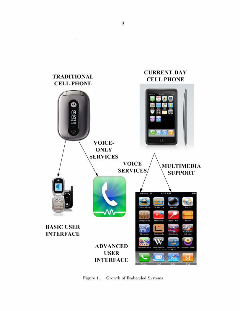
The complexity of current-day embedded systems is explained using Figure 1.1.

To give a brief introduction, ’Scheduling’ is the method by which threads or processes are given

access to system resources (processor time, memory, I/O channels). The processor software

component which is in charge of scheduling is called ’Scheduler’. In general, the aim of the

process/thread scheduler is to increase system throughput, maximize CPU utilization or to

ensure fairness among applications. In some cases, it could be minimizing metrics such as

Turn- around time, power, energy etc. Since modern day embedded systems work in a highly

dynamic environment, it is difficult to predict in advance the applications that will be run

and their resource requirements. The computational load in the system is data-dependent

and varies with respect to time and number of tasks in the system. We proceed further and

describe the concepts that help us define a polymorphic embedded system.

1.1 Polymorphic Computing System

In this section, we define and specify a polymorphic embedded system, a futuristic approach

for embedded system design. Before defining what a polymorphic thread system, we need an

efficient way for representing operating system tasks. Scheduling can be accomplished at differ-

ent granularities, course level(application level) or at fine grained level(threads/process) level.

Threads are optimized representation of tasks, due to their low context switching overhead.

Since modern day processors offer extensive support for multithreading, task scheduling is ac-

complished at thread level granularity. Also, thread level resource information is considerably

high compared to other task representations. Due to these compelling reasons, applications

are examined at thread level granularity in the proposed scheduler framework.

The origin of the word ’Polymorphism’ comes from words ’Poly’ and ’Morph’. Morphism is

the quality of taking up a particular form or shape. The word ’Poly’ means Multiple and

3

Figure 1.1 Growth of Embedded Systems

4

hence the term ’Polymorphism’ stands for multiple forms. The notion of morphism is similar

to Design Space Exploration. Design space exploration is the process of examining several

implementation choices, which are functionally similar, in order to identify an optimal solu-

tion. The threads within an application can be implemented in a multitude of ways, where

each thread’s implementation is referred to as morphism. A polymorphic embedded system is

one which supports execution of multiple multithreaded applications. The scheduler for such

a system has to efficiently choose morphisms for the threads lined up for execution in the

ready queue. The morphism choices for the threads, depends on the instantaneous resource

availability. Chapter 2 elucidates the concept of morphism in finer detail.

1.2 Novelty of Proposed Work

This is the pioneer attempt at designing a thread scheduler for a polymorphic embedded sys-

tem. None of the existing literature on thread scheduler design has accounted for thread

polymorphism. We describe the novelty and performance advantages of the proposed system

versus conventional high performance embedded systems. In the case of conventional high

performance embedded systems, makeup of applications is known at design time. We further

describe how the existing scheduling strategies tackled the resource allocation problem.

Priority scheduling has been predominantly employed for task scheduling in conventional sys-

tems VxWorks [1997], QNX [1999]. The traditional models for resource allocation, in real-

time embedded systems are based on periodic or sporadic execution model. C.L.Liu et Al.

[1973], Mok [1983], Spuri et Al. [1994], Buttazo et Al. [1995] discuss about the aperiodic and

sporadic resource allocation models. In the case of Rate Monotonic Scheduling(RMS)

scheme, tasks which have high recurrence rates receive precedence over tasks with low fre-

quency rates. The RMS scheduling approach is detailed in C.L.Liu et Al. [1973] Lehoczky

[1989]. In the Earliest Deadline First(EDF) scheduling strategy, the scheduler must ensure

that all tasks complete execution before their specified deadlines. Spuri et Al. [1994] Leung et

5

Al. [1982], elaborate about the Earliest Deadline Scheduling(EDS) technique. But the priority

scheduling scheme used in the EDF and RMS schemes, suffers from a number of shortcomings.

In the case of static priority scheduling, tasks are assigned priorities which remain the same

throughout the task’s execution. Priority scheduling performs badly for tasks whose run-time

behavior deviates significantly from its expected or design time behavior. Moreover the be-

havior of these tasks may vary with respect to time and the number of tasks in the system.

Another drawback in priority scheduling is that there is no foolproof mechanism for mapping

task requirements into priority values. In many cases, the system designer accomplishes this

mapping based on a pre-determined set of facts. The user-satisfaction based resource allocation

scheme employed by the proposed polymorphic thread scheduler addresses the above issues,

offering significant performance benefits over classical scheduling schemes.

Hybrid Reconfigurable Systems(HRS), an emerging trend in current embedded system

design has CPU cores and reconfigurable fabric on a single die. Programming models for hy-

brid CPU/FPGA systems were studied in D.Andrews et Al. [2004] Peck et Al. [2006]. In

these systems, the scheduler categorizes a thread as either software or hardware. But the de-

sign choices for the scheduler are limited in these systems. The polymorphic embedded system

explores a much bigger design space, by considering several functionally equivalent software im-

plementation alternatives for a given thread. In conventional embedded systems, the makeup

of applications is known at design time and the user has no way of dictating priority for the

applications. But in the proposed polymorphic embedded system, application characteristics

are known only at run time. Unlike conventional systems, where the objective is to increase

performance, reduce energy or power, the proposed polymorphic scheduler places an emphasis

on increasing user satisfaction. In any typical embedded system, human perception matters

the most. This is because of the fact that, user perception is a clear indicator of application

performance. Since there are limits to human perception, there are upper and lower limits to

the user satisfaction function. Considering an illustration, let the end-user be watching a video

at DVD clarity. The user satisfaction in this case, would have reached the upper saturation

6

limit and any further increase in video quality, doesn’t significantly alter user satisfaction. The

lower limit is the point, below which there is zero user satisfaction. There is a middle region,

where there is non-linear increase in user satisfaction with increase in performance metric. The

upper limit is the region beyond which, no pronounced increase in user satisfaction is achieved

with increase in resources.

In order to capture user perception, we require a function which holds similar properties. The

Sigmoid function is an S-shaped knee curve with near-linear central response and saturating

limits. The novelty in our approach compared to prior work is that, sigmoid function is used

for modeling user satisfaction. The function helps us to establish the Lower/Upper limit or

Desired Operating Points (DOP). Desired Operating Point is the region in the sigmoid curve,

above which marginal user satisfaction gain is imperceptible to the end user. Resources to

enhance output parameter (User satisfaction) is not proportional to actual/perceived enhance-

ment. This is the principal reason behind choosing sigmoid function to model user satisfaction.

This is the advantage of the proposed system over conventional systems, which have no clear

way of establishing the Desired Operating Points. To summarize, the thesis work, a dy-

namic thread scheduler which effectively functions in a multiple application, multithreaded

polymorphic environment has been implemented and evaluated. The rest of the thesis is orga-

nized in the following manner.

The related work for the thesis is summarized in Chapter 2. Chapter 3 discusses the pre-

liminary concepts, which form the basis for our scheduler framework. Chapter 4 describes

the data structures for the scheduler and explains how resource contention is modeled using

marginal utility approach. Chapter 5 elaborates on the proposed greedy scheduling algorithm

and discusses the scheduling heuristics implemented. Chapter 6 presents a methodology for

performance evaluation and testing of the polymorphic scheduler framework. This chapter

details the algorithm for generating random graphs, which serve as benchmarks for testing the

proposed scheduler framework. Chapter 7 discusses the experimental setup and the simulation

7

results, which demonstrate the performance benefits of the proposed greedy scheduler algo-

rithm over classical scheduling schemes.

8

CHAPTER 2. Related Work

The related work for the thesis can be categorized into three main classes. The first class of

literature is about the usage of sigmoid function for modeling user satisfaction in mobile sys-

tems. The polymorphic thread scheduler proposed in thesis, employs the sigmoid function to

capture user satisfaction changes. The second class of literature explores the design techniques

for Hybrid Reconfigurable Systems (HRS), an emerging trend in high performance embed-

ded computing systems. The third class of papers discuss about admission control, which is

implemented as part of the resource allocation strategy in an embedded system.

2.1 Hybrid Reconfigurable Systems

Embedded domain applications require high computing power. Jason et Al. [2006], proposed

the methodology to migrate application portions to custom hardware or ASIC (Application

Specific Integrated Circuit). Hybrid Reconfigurable System (HRS) is the ideal computing

platform which supports execution of a diverse class of applications. These systems have

reconfigurable fabric interspersed with high performance CPU cores. Hence, programming

models and operating system support for Hybrid Reconfigurable Systems (HRS) has gained

a lot of interest in the embedded systems community. Traditional programming models and

operating systems for hybrid systems have treated CPU cores as masters and the reconfig-

urable fabric as slaves. Recently proposed programming models such as H-threads model in

D.Andrews et Al. [2004] Peck et Al. [2006], have introduced the concept of abstraction at the

process level for Hybrid Reconfigurable systems. The H-threads programming model abstracts

the FPGA/CPU components to form a custom unified multiprocessor architecture platform.

Hence the designer is freed from specifying and embedding platform specific instructions for

9

communicating across the Hardware/Software Interface.

David et Al. [2005] talks about the design of a multithreaded RTOS kernel Hthreads - for

Hybrid CPU/FPGA systems. Jason et Al. [2006] discusses the methodology used by the sched-

uler to execute software threads and threads implemented in programming logic. The essential

feature with this model is that Operating System thread services such as Thread Management,

Thread Synchronization Primitives, and Thread Scheduling components are moved to hardware

to support scheduling of threads across the Hardware/Software Boundary. The other relevant

works on Operating System design for Hybrid Reconfigurable Systems (CPU/FPGA Hybrid

systems) is discussed in Nollet et Al. [2003], Mignolet et Al. [2003], Nollet et Al. [2008]. The

papers on Hybrid Reconfigurable Systems, do not account for thread polymorphism. In these

systems, the design space for the scheduler is limited, as the scheduler can categorize a thread

only as software or a hardware thread. This voids out the advantages that might be offered

by investigating other design spaces. In general, the embedded system designer can realize a

thread’s functionality using different algorithms. In other words, a thread can have multiple

software morphisms. The polymorphic thread scheduler helps the embedded system designer

explore such design spaces. The concept of thread morphism and its associated benefits are

examined in greater detail in Chapter 3.

2.2 Literature on Sigmoid Function

In our polymorphic thread scheduler design, the objective function to be maximized is user

satisfaction. We accomplish the task of maximizing user satisfaction by modeling it using

the sigmoid function. Chapter 3 talks in detail about how user satisfaction is modeled using

sigmoid function.

The work by Nicholas et Al. [2003] Sourav et Al. [2005] have used sigmoid function for model-

ing user satisfaction. The effectiveness of sigmoid function lies in modeling variations between

user satisfaction and service quality as mentioned in Xiao et Al. [2001], Stamoulis et Al. [1999].

10

Depending on the Quality of Service (QOS) offered to an application, the corresponding user

satisfaction changes. Ahmad et Al. [2005] addresses the issue of increasing user satisfaction by

preempting resources from other applications. When higher priority applications need to be

executed, lesser privileged applications are preempted. Sourav et Al. [2005] Pal et Al. [2005]

model user satisfaction/dissatisfaction using user irritation, i.e., the amount of performance

degradation or delay the user is willing to tolerate. Alpha is the parameter denoting service

quality in the sigmoid function. It is also a measure of user sensitivity to performance degrada-

tion. Hence for premium users, parameter alpha’s value is higher as users are willing to pay a

high price for a service and these users are more sensitive to performance degradation. Nicholas

et Al. [2003] proposes a Radio resource allocation strategy and discusses how sigmoid function

is used for modeling the user satisfaction for the different class of users. Current day mobile

phones, in addition to traditional voice services, offer a broad range of multimedia application

support to mobile users. In order to accommodate both these class of services, an efficient

resource management and allocation scheme as presented in Sampath et Al. [1995] Zhao et

Al. [2002] is needed. The users are categorized into different classes depending on the rev-

enue paid. Sourav et Al. [2005] Pal et Al. [2005] classify the traffic for user applications into

conversational, interactive and background. Each user class supports all services with differ-

ent commitment depending on the delay, the user is willing to tolerate for each traffic class.

Other relevant approaches such as Zhao et Al. [2002], Liang et Al. [2002], propose resource

management schemes for future generation wireless networks.

2.3 Literature on Admission control

In real time systems, admission control determines the feasibility for task scheduling. Admis-

sion control is a process which determines how to allocate network resources, e.g. bandwidth

to different applications. An application that wishes to use the network’s resources must first

request a QOS connection, which involves informing the network about its characteristics and

QOS requirements. If there are sufficient resources in the network to guarantee the QOS level,

then the application is admitted into the system. Admission control is implemented in the

11

first phase and the second phase reserves bandwidth and does resource allocation to admitted

requests. Pal et Al. [2005], Zhao et Al. [2002] present radio resource management schemes

which implements admission control Pellizoni et Al. [2007]. Admission control is also imple-

mented in the polymorphic scheduler, where threads are admitted into the system based on

their contribution to the user satisfaction function. We elaborate about how admission control

is implemented in our scheduler in chapter 5. In the next chapter, i.e. Chapter 3, we intro-

duce the underlying concepts and formulate objective function for the polymorphic embedded

system.

12

CHAPTER 3. INTRODUCTION

3.1 Concept of Morphism

Let us introduce the concept behind morphism in this section. Morphism is the property to

take up a specified form. In other words, morphisms are alternate ways of implementing a

thread’s functionality. A thread’s morphism decides the resource consumption for a thread

and its contribution to the application’s performance metric. The morphisms differs in their

resource requirements to realize a thread’s functionality. For illustration, let us assume a thread

has three morphisms. The first thread morphism can be tuned for faster execution, second

optimized for memory storage, while the third might be designed to operate in a power-saver

mode. Moreover, a thread’s behavior could be implemented in software/hardware. Multiple

software implementations possible for a thread by changing the algorithm used to realize a

thread’s functionality.

Morphism selection can be done at different levels such as (Algorithm or Design level), Source

code Level, Compile level etc. For instance if a thread needs to perform sorting, heap sort,

merge sort and quick sort are the different design choices. Let us assume that we picked

one among these design choices at the source code level. At the source code level, parallel

and sequential code implementations of a procedure form the different morphisms. At the

compile level, compiler optimized versions of the same program are the various morphisms.

Hence, there is a close analogy between thread morphisms and software optimization. Soft-

ware optimization involves modification of a software system aspect for efficient execution or

for consuming fewer resources. Similar to morphisms, software optimization can be carried out

at various levels such as at Algorithm, source code level etc.

13

Let us demonstrate the concept behind thread morphisms using an illustration. For instance,

given below is a for loop to add two arrays of size 1000 and store it in a third array.

for i = 1 to 1000 do

c[i] = a[i] + b[i]

end for

The for loop where the index variable runs from 1-1000 can be executed serially on the func-

tional units of the processor. This constitutes one morphism, or way of executing the procedure

onto the processor. Another morphism could be that the loop can be parallelized and exe-

cuted on a vector adder unit. Depending on compiler optimizations available and also based

on resource availability, one among these two morphisms will be chosen at run time. Consider

the following C code snippet, whose purpose is to obtain the sum of all integers from 1 - N .

for i = 1 to N do

sum+ = i;

end for

Assuming no arithmetic overflow, the above code can be rewritten efficiently using a mathe-

matical formula sum = (N ∗ (N + 1)) >> 1. We see that >> 1, is right shift by 1, which

is equivalent to divide by 2 when N is non-negative. Our choice of the algorithm version,

depends on the problem size N . For lower values of N the first morphism version is preferred

over the second. This is because, the looping operation takes lesser time to execute compared

to the multiplication and bit-shifting hardware time complexity. As the value of N increases,

the second version might be opted.

Morphism of a thread plays a role in determining how much a thread’s implementation enhances

the performance metric. Each thread morphism differs in its resource requirements in order

to realize a thread’s behavior. The scheduler decides on the appropriate morphism choice

for a thread depending on current resource availability and the thread’s relative priority. For

14

instance, some morphism might achieve considerable reduction in execution time, but at the

price of making it consume more memory. In systems where memory is at a premium, a

morphism which consumes less memory is preferred over the other morphisms. Modern day

processors have Graphic Processor Units (GPU), Field Programmable Gate Arrays (FPGA),

CPU and other heterogeneous computing units. The motivation of the morphism problem

in such cases, is to come up with the ideal system design, which includes the proper mix of

processor units, FPGA and GPU units in order to achieve enhanced user satisfaction. The

next section elaborates on user satisfaction and how it is modeled using the sigmoid function.

3.2 Performance Assessment in Embedded System

In an embedded system, user input is provided usig an input device such as mouse or pen and

output can be realized using LCD Display and speakers. In any typical embedded system, it is

human perception that matters the most. Unlike many conventional embedded systems, where

the objective of the system is to increase performance, reduce power or energy consumption, our

system plays an emphasis on increasing user satisfaction. In conventional embedded systems,

the makeup of applications is known at design time and the user has no way of dictating

priority for the applications. This is exactly where our scheduling algorithm differs in its

objective. The scheduler dynamically schedules threads from multiple applications with the

intent of maximizing user satisfaction. The marginal increase in user satisfaction per unit

resource decides application priority. This is because of the fact that user perception is a

clear indicator of application performance. Since there are limits to human perception, there

are upper and lower limits to the user satisfaction function. There is a lower limit on the

perception of human eye, or lower knee below which there is zero or no user satisfaction.

There is a middle region, where there is non-linear increase in user satisfaction with increase in

performance metric. Voice perception coupled with perceptible frequency range exhibits these

characteristics. In order to accurately capture user experience, user satisfaction is modeled

using sigmoid function, which is illustrated in the subsequent section.

15

3.3 Modeling User Satisfaction

Lower Knee In any embedded system, user-perceived satisfaction, which is a function

of the application throughput, is what matters the most. The aim of an embedded system

designer, is to maximize this user-perceived satisfaction. Since there is a limit to the perception

of the human senses, there is a lower bound on the performance metric, below which, there is

zero or no user satisfaction. In other words, this marks the lower threshold of the performance

metric, below which human perceived satisfaction is zero as shown in Figure 3.1.

Upper Knee In a similar manner, human eye cannot distinguish marginal user satisfac-

tion increase obtained due to additional performance gains beyond a particular point. This

establishes the upper bound or the upper knee in the S-shaped sigmoid curve, corresponding

to a sigmoid function as shown in Figure 3.1. Above this region, the user is unable to perceive

any notable increase in performance.

Middle Region Also there is a middle region between these lower and upper thresh-

old values, where the marginal increase in user satisfaction exhibits non-linear behavior with

increasing values of performance metric. Voice perception, audio and video applications ex-

hibit this behavior. Sigmoid function captures the user experience for all these applications.

The User Satisfaction function, represented by u(t), modeled using the sigmoid function has a

characteristic S-shaped curve whose equation is as follows.

u(t) =1

1 + c0 e−c1t

s

In the above equation c0, c1 are constants. The term t in the expression for sigmoid function,

represents the normalized throughput. Throughputmax is the maximum throughput among

all the thread morphisms. Throughputmin is the thread morphism with minimum throughput.

Throughputmid is the thread morphism with median throughput. Normalized throughput t,

where −1 ≤ t ≤ 1 is given by the following expression. Since normalized throughput is the

16

parameter in the sigmoid function, user satisfaction is a function of normalized throughput.

The normalized throughput value helps in achieving a bounded value for sigmoid function, due

to convergence of Taylor series. Throughput information is provided by the embedded system

designer in form of a morphism table, which is discussed in Chapter 4.

t =Throughputcur − Throughputmid

Throughputmax − Throughputmin

The value of sigmoid function is bounded between 0 and 1. For illustration let a user be watch-

ing or playing a movie with DVD clarity. In this case, user satisfaction would have already

reached its peak and any further increase in clarity is unlikely to be perceived by the end

user. This point is chosen as the upper threshold. Beyond this point, there is no significant

increase in user satisfaction, with increase in application’s performance metric. The sigmoid

function clearly captures that behavior and another reason for choosing this function is be-

cause it is defined at all points for parameter t. The sigmoid function therefore helps in clearly

establishing the lower and upper bounds for performance metric. This is an advantage over

conventional systems, where there is no clear way to establish these performance metric bounds.

The parameters of the sigmoid function can be either discrete or continuous. In the case of

video applications, the frame rate is a discrete parameter, since digital video sampling is done

at discrete intervals. On the other hand, webpage loading delay is an example of a continuous

parameter. Frame rate is one of the parameters which helps capture user experience in the

case of visual multimedia applications such as video chatting, teleconferencing etc. A video

player plays movie files/DVD can have a frame rate of 15 frames/sec (fps) to 30 fps in steps of

2 fps. 3D Gaming applications need 30 fps to 60 fps in steps of 5 fps and video chatting has

frame rate of 3 fps to 15 fps. The diagram illustrated in Figure 3.1 shows the plot of the user

satisfaction function versus the application’s performance metric namely throughput.

17

Figure 3.1 User Satisfaction Plotted Against Throughput

3.3.1 Approximation of sigmoid function

In the sigmoid equation, let us assume values for constants, c0 = 1, and c1 = 1. The value of

the sigmoid function can be approximated using the following Taylor series expansion.

1

1 + e−t=

1

2+t

4− t3

48+

t5

480+ . . .

Since we know that −1 ≤ t ≤ 1, and the scheduler must make decisions quickly, we can

approximate the value of the user satisfaction by considering the first N terms. The value of

N is decided, based on the precision desired for the system and the time taken to compute the

approximation. Fixing the optimal number of terms, would speed up scheduling decisions and

give us the right precision. In general, since the scheduling algorithm itself should not be an

overhead, the first three or four terms in the Taylor series expansion are considered to evaluate

the user satisfaction function. In the next section, we describe the Application model used in

18

the Polymorphic thread scheduler. The Application model depicts a typical state scenario in

any embedded system.

3.4 Overview of Application Model

The system framework consists of N multithreaded applications A0, A1 . . . An−1, with each

application Ai having pi threads. The morphism space for thread Ti,j 0 ≤ j < pi is denoted

by Ti,j,r where 0 ≤ r < mi,j . Here mi,j denotes the morphism space for the thread Ti,j .

3.4.1 Application State Transition Graph

In this section, we introduce the notion of an Application State Transition Graph (ASTG),

to capture the asynchronous nature of external events in an embedded system. Here, a state

is labeled with an n-bit vector, where the ith bit represents if application Ai 0 ≤ i < n is

active or not. In general, only a fraction of the entire space of 2n states are feasible, due to the

design constraints enforced by the embedded systems designer. The embedded system design

is greatly simplified, as the resource allocation problem has to be solved at each state in the

Application State Transition Graph(ASTG).

Let us consider an Application State Transition Graph as shown in Figure 3.2. For illustration,

we study the case with two applications in the embedded system, namely video and phone.

We have four states in the system namely S0,S1,S2,S3. Initially the system is in the idle

or start state S0, which reflects no user activity. When the user wants to watch a video or a

movie, a state transition occurs from state S0 to state S1 where, only the video application is

active. When the system is in state S0, and if the user receives a phone call, a state transition

occurs to state S2. This is an indication, that the user is attending a phone call and is not

engaged in any other activity. When the user is watching a video, and if there is a phone call,

the system allows both these applications to co-exist and transitions to state S3. The next

section describes scheduling in Real time systems and discusses in detail about polymorphic

thread scheduling.

19

Figure 3.2 Illustration of Application State Transition Graph

3.5 Scheduling in Real-time Systems

In Real time systems, admission control decides the feasibility for task scheduling. If a certain

level of QOS or minimum level of QOS cannot be guaranteed for a thread, it is not admitted

into the system. The application wishing to be scheduled onto the processor, informs the

processor about the characteristics of its computational load and its desired level of QOS. The

thread scheduler corresponds with the resource allocation layer and decides whether to admit

or reject the application’s request to enter the ready queue. If resources are not available to

guarantee a certain level of QOS, the task is not admitted. The task is admitted at some

later point of time when the system has sufficient resources. The objective here is to ensure

execution of tasks which have stringent deadlines. In general, the feasibility for scheduling a set

of tasks together is decided by their execution times and deadlines. Examples of some of the

20

scheduling strategies are Earliest Deadline First, Rate Monotonic Scheduling(RMS), Shortest

Job First(SJF) etc. The objective function in these strategies is to maximize the number of

tasks admitted into the system.

3.6 Polymorphic Thread Scheduling

Thread scheduling poses a lot of challenges in a polymorphic embedded system environment.

The scheduler has to deal with two cases which might arise during scheduling. Let us discuss

the motivation behind polymorphic thread scheduler design by considering a simple scenario

of running a single multithreaded application in the system. We then generalize the approach

for N multithreaded applications running in the system. In both these cases, the scheduler

has to choose a common optimization metric across applications.

3.6.1 Single Application Scenario

The scheduler decides to optimize the performance metric for that application e.g. Maximize

System throughput. When there is resource contention among threads, the thread with higher

marginal increase in performance metric is given precedence over others.

3.6.2 Multiple Application Scenario

The scheduler design for a multiple application multi-threaded scenario becomes a lot complex.

When multiple applications are active, with each application consisting of multiple threads, the

question is which thread from which application is to be scheduled. The problem’s complexity

increases when there is more than one morphism implementation is possible for a thread. The

aim of the scheduler is to come up with the correct morphism choices for the different threads

to be scheduled. Hence the scheduler’s job is to decide the admissible set(threads which can be

admitted into the system) as well as come up with morphism choices for ready-to-run threads.

21

3.6.3 Need for Objective Function

We need a common metric to help us determine the marginal utility of scheduling a thread per

unit resource. We formulate an objective function for the multithreaded multiple application

framework, with user satisfaction as the optimization metric. The objective function aids in

making resource allocation decisions and establishes the underlying application model. We

introduce the concepts of thread control flow graph and scaling factor in following section,

which forms the basis for the thread scheduler’s objective function.

3.7 Thread Control Flow Graph

We build the objective function S for a single multithreaded application. The scheduler chooses

to optimize the performance metric for an application, e.g. System or network throughput.

Throughput is expressed in terms of frames/sec or network throughput B/sec. The scheduler’s

goal is to maximize this throughput at the sink node. This is because of the fact that an appli-

cation’s actual user satisfaction can be perceived only at the sink node In our system, a subset

of N multithreaded applications can be active at any time instant. A single multithreaded

application’s functionality can be represented using a data structure called as thread control

flow graph. The graph clearly captures the computational and communication flow between

threads constituting an application. Nodes in the graph represent the threads and the edges

between nodes at different levels denote the scaling factor corresponding to each thread. Each

Application Ai, 0 ≤ i < n consists of pi threads Ti,j , 0 ≤ j < pi. Each of these threads are

designed by application designers for multiple morphisms. The morphism space for a thread

Ti,j is represented by mi,j , 0 ≤ r < mi,j .

3.8 Scaling Factor

Let us introduce the notion behind scaling factor associated with a particular thread. The

scaling factor determines the number of computational units of a particular thread required

to generate one computational unit of output information at the sink node. For instance if 1

frame at the output of a thread Ti,j , results in 1 frame at the output of the sink thread scaling

22

factor si,j = 1. If f(Ai) represents the performance metric for application Ai, the aim of the

local optimization function is to maximize si,j ∗ f(Ai). An application’s actual user satisfac-

tion is perceivable only at the sink node in the thread control flow graph and the scheduler’s

goal is to maximize the same. Therefore the maximization of performance metric problem, is

mapped into a local optimization problem. Since the scaling factor is a normalized metric, for

any thread j, 0 ≤ j < pi, we have 0 ≤ s0,j,k ≤ 1. Here k denotes the edge associated with a

particular thread j. If the total number of outgoing edges from thread j is e then 0 ≤ k < e.

Recall the fact that, morphism corresponds to the different ways of implementing a particular

algorithm choice. The scaling factor for a thread is dependent only on the algorithm choice

and not on morphism selection. Moreover, it decides a thread’s relative contribution to the

overall throughput. It is dependent on the design algorithm choice and remains unaffected by

morphism changes. Morphism of a thread decides the per unit time notion of the performance

metric. Morphism has zero effect on the scaling factor and morphism changes affect the

individual thread’s throughput and also system throughput. Let us better understand this

fact with an illustration.

3.8.1 Illustration - Scaling Factor

Let us illustrate how scaling factor and morphism are independent of each other. Consider

four equal sized jobs assigned to 4 strong individuals. Four equal sized jobs are assigned to 4

strong individuals. The jobs cannot be shared among people and each person is responsible

for completing the task assigned to him. Assuming that one among these strong persons falls

sick, we replace him by a weaker individual. Observe that the amount of work assigned to the

person remains the same, irrespective of the nature of individual. In other words, the workload

assigned to a person remains constant, regardless of the physical stature of the person. When

a person is exchanged in place of another, the time taken to complete the task changes thereby

affecting system performance.

23

3.8.2 Analogy with morphisms

Drawing similarity between the previous illustration and morphisms, tasks are analogous to

threads. The work expected from each person is comparable to the thread throughputs. The

switch in person’s nature is similar to switch in a thread’s morphism. When a person’s na-

ture changes from strong to weak, it affects the task’s throughput. Similarly when a thread

undergoes a morphism change, there is a corresponding throughput change affecting system

throughput. The figure 3.3 illustrates the above analogy with the strong-weak example. The

concepts relating to thread control flow graph and scaling factor have been explained. The

following section makes use of these concepts to formulate the objective function for the poly-

morphic thread scheduler.

Figure 3.3 Independence of Scaling Factor and Morphisms

24

3.9 Objective Function

We adopt the following approach to model the system behavior. As the first step, we model

the behavior of a single multi-threaded application and then generalize the approach to model

the system behavior of N applications. An application A0’s functionality, represented by a

thread control flow graph is illustrated in Figure 3.4. The nodes in the graph represent the

threads and the edges denote the scaling factors associated with the threads. Since the scaling

factor is a normalized metric, for any thread j, 0 ≤ j < pi, we have 0 ≤ s0,j,k ≤ 1. Here k

denotes the edge associated with a particular thread j. If the total number of edges in the

graph is e then 0 ≤ k < e. One interesting fact to note is that, a thread’s contribution to the

overall application throughput is dependent on the threads and edges which are active at any

time instant(active cut). From Figure 3.4, it is evident that a thread could be part of several

cuts at different time instants. For instance, both the threads T0,1 and T0,2 are part of cuts C1

and C2.

Let us consider a single multithreaded application A0 having pi threads, T0,j for 0 ≤ j < pi.

Let the performance metric be throughput, for these threads, denoted by Throughput(T0,j).

A thread’s throughput can be decided only when a corresponding morphism has been selected

for it. The morphism space or the maximum number of morphisms possible for a thread Ti,j

is denoted by mi,j . Let us find out a thread’s contribution to the overall performance metric.

As we mentioned earlier, this depends on the threads in the application, which are lined up

for execution in the ready queue. The sink node in the thread control flow graph is where

the user satisfaction for an application can be perceived. Since we cannot exactly determine

an application’s user satisfaction, a greedy approach is adopted, where the sensitivity of the

currently executing threads is maximized. Hence, the maximization problem of performance

metric translates into a local optimization problem, where we approximate the effect of cur-

rently executing threads on the application’s actual user satisfaction.

Let the threads present in the cut C2 for application A0 be active. Hence, threads T0,1, T0,2, T0,5

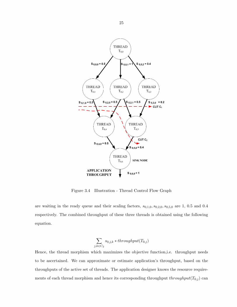
25

Figure 3.4 Illustration - Thread Control Flow Graph

are waiting in the ready queue and their scaling factors, s0,1,0, s0,2,0, s0,5,0 are 1, 0.5 and 0.4

respectively. The combined throughput of these three threads is obtained using the following

equation.

∑j,k∈C2

s0,j,k ∗ throughput(T0,j)

Hence, the thread morphism which maximizes the objective function,i.e. throughput needs

to be ascertained. We can approximate or estimate application’s throughput, based on the

throughputs of the active set of threads. The application designer knows the resource require-

ments of each thread morphism and hence its corresponding throughput throughput(T0,j) can

26

be determined using a table lookup. Let us determine thread T0,2’s relative contribution to

the overall throughput considering that cut C2 is active.

s0,2,0∑j,k∈C2

s0,j,k∗ throughput(T0,2) =

0.5

1.9∗ throughput(T0,2)

The value computed above, is the contribution of thread T0,2 to the overall throughput and

varies for each morphism r where 0 ≤ r < mi,j , denoted by throughput(T0,2,r). If the

thread T0,2 is part of another active cut, namely C1, where the scaling factors for the threads

are 0.5, 1, 0.2 for threads T0,1, T0,2, T0,3 respectively, thread T0,2’s contribution to the overall

throughput is as follows.

s0,2,0 + s0,2,1∑j∈C1

s0,j∗ throughput(T0,2) =

1

1.7∗ throughput(T0,2)

Let us restate the maximization problem in terms of the throughput of a thread morphism,

namely throughput(T0,j,r). Our aim is to maximize the objective function given below.

S =∑pi

j=0

∑m0,j−1r=0 s0,j,k ∗ throughput(T0,j,r) ∗Ready(T0,j) ∗M0,j,r.

Ready(Ti,j) =

1 if thread j is in ready to run

0 otherwise

M0,j,r is a Boolean variable, which represents if morphism r of a thread j is active or not in the

current scheduling cycle. Value of M0,j,r = 1 if thread T0,j assumes morphism r, 0 ≤ r < m0,j ,

in the current scheduling cycle. Otherwise M0,j,r = 0, if the thread does not assume this

morphism. Maximum number of morphisms possible for a thread is given by m0,j . In general,

the performance metric for a thread is denoted by f(T0,j). The performance metric makes

more sense, when it is specific to a thread morphism and is denoted by f0,j,r. The objective

function can be modified as follows.

S =∑pi

j=0

∑m0,j−1r=0 s0,j,k ∗ f0,j,r ∗Ready(T0,j) ∗M0,j,r

27

3.9.1 Constraints

The scheduling algorithm is bound by certain constraints at run time. Constraint one is that,

the scheduler also has to ensure that at most only one morphism for a thread can be active dur-

ing a scheduling cycle, by enforcing a constraint on the value of M0,j,r, i.e.,∑m0,j−1

r=0 M0,j,r ≤ 1,

where ∀j, 0 ≤ j < pi.

Also another constraint that must be obeyed is, the sum of the total number of resources of each

type allocated to all the active threads in the application can never exceed the total number

of resources present in the system. If we have q different resource types present in the system

ranging from R0, R1 . . . Rq−1 where each resource type can represent memory, processing units

or I/O devices. If resi,j,r,a, represents the number of resource units of type Ra allocated to

thread j 0 ≤ j < pi in application A0, where resource type a ∈ {0, 1, 2 . . . q − 1}, the second

constraint is as follows.

∑j,r

M0,j,r × res0,j,r,a ≤ Ra∀a ∈ {0, 1, 2 . . . q − 1}

3.10 User Satisfaction as Objective Function

From the Application State Transition Graph(ASTG), we can generalize the relative through-

put contribution of a thread. If we have a single application A0, then each thread l’s relative

contribution is given by the following equation, 0 ≤ l < pi. Here k′ represents the set of

outgoing edges from thread l, part of the active cut C1.∑k∈k′ s0,l,k∑

j,k∈C1s0,j,k

∗ throughput(T0,l).

We can restate objective function in terms of user satisfaction function, which we want to

maximize using the following expression.

USat =pi∑j=0

∑k∈cut

m0,j−1∑r=0

s0,j,k ∗ UserSat(NormalizedThrput(T0,j,r) ∗Ready(T0,j) ∗M0,j,r

UserSat(NormalizedThrput(T0,j,r)) denotes the normalized user satisfaction increase ob-

tained due to a thread morphism and is given by the following expression.

28

USat =pi∑j=0

∑k∈cut

m0,j−1∑r=0

s0,j,k ∗ UserSat(NormalizedThrput(T0,j,r)) ∗Ready(T0,j) ∗M0,j,r

Hence substituting the Sigmoid function for the User Satisfaction function, we have the fol-

lowing expression.

USat =pi∑j=0

∑k∈cut

m0,j−1∑r=0

s0,j,k ∗1

1 + eThrput(T0,j,mid)−Thrput(T0,j,r)

Thrput(T0,j,max)−Thrput(T0,j,min)

∗Ready(T0,j) ∗M0,j,r

Generalizing the above expression for N applications in the system, we have the following

equation.

USat =N−1∑i=0

pi∑j=0

∑k∈cut

mi,j−1∑r=0

si,j,k ∗1

1 + eThrput(Ti,j,mid)−Thrput(Ti,j,r)

Thrput(Ti,j,max)−Thrput(Ti,j,min)

∗Ready(Ti,j) ∗Mi,j,r

29

CHAPTER 4. MARGINAL UTILITY APPROACH

4.1 Scheduler Data Structures

The sections in this chapter are organized in the following manner. The first section details

the data structures maintained by the scheduler and the constraints for operation of the poly-

morphic thread scheduler. The subsequent sections introduce the idea behind Marginal Utility

Scheduling and elucidate it in finer detail. The scheduling algorithm has tables as data struc-

tures, in order to maintain information about the different thread morphisms. Any application

thread requires resources for execution, in order to produce a certain throughput. Since these

tables store morphism information for the different application threads, the data structure is

called morphism table. Morphism tables are maintained for each thread j, 0 ≤ j < pi, for every

application Ai, 0 ≤ i < n in the system. The entries in the morphism table are sorted in de-

creasing order of their performance metric (throughput). Hence, the first row in the morphism

table corresponds to the thread morphism which yields maximum throughput. The columns

in the morphism table are as follows. There is a column to index the different morphisms for

a thread and the subsequent columns store details about the amount of resources required for

its execution and throughput of the thread morphism. The resources in the system could be

the amount of Random Access Memory (M) required, Disk Memory (D) and Processing Units

(P ), which form the various columns M,P,D in the morphism table. The application designer

can statically estimate the needs of the thread morphisms and sort the entries in the table

in decreasing order of the throughputs. The constraints for the scheduling algorithm are as

follows.

The scheduler algorithm is bound by 2 constraints. Constraint 1 is as follows. A thread can

30

be assigned a maximum of one morphism r, 0 ≤ r < mi,j . The morphism space for thread Ti,j

is denoted by mi,j . Hence, a morphism table for a thread has a total of mi,j rows or morphism

entries. Mi,j,r is a Boolean variable, which represents if morphism r of a thread j is active or

not for Application Ai in the current scheduling cycle. Value of Mi,j,r = 1 if thread Ti,j assumes

morphism r, 0 ≤ r < mi,j , in the current scheduling cycle. Otherwise Mi,j,r = 0, if the thread

does not assume this morphism. Constraint 1 is given by the equation∑mi,j−1

r=0 Mi,j,r ≤ 1,

∀i, j. Constraint 2 states that the sum of resource requirements for thread morphisms must

never exceed the total resource limit. The above statement must hold good for every resource

type present in the system. The total number of resource types in the system are denoted by

q, with each resource type denoted by Ra,a∈ {0, 1, 2 . . . q− 1}. If (M,P,D), denotes resources

present in the system, memory requirements of currently running thread morphisms should

never exceed the total available memory in system. The same constraint should be enforced,

for the other resource types in the system namely Processing Elements and Disk Memory. If

Ri,j,r,a, represents the number of resource units of type Ra allocated to thread j, 0 ≤ j < pi in

an application Ai, 0 ≤ i < n, the second constraint is as follows.

∑i,j,r

M0,j,r ×Ri,j,r,a ≤ Ra∀a ∈ {0, 1, 2 . . . q − 1}

4.2 User Sensitivity

In this section, we introduce the concept behind user sensitivity, before describing how resource

contention is modeled in a multiple application multithreaded scenario. In any embedded sys-

tem, human perception is the actual measure of user satisfaction. The sink node in the thread

control flow graph is where, the actual user satisfaction for an application can be perceived.

But in any scheduling cycle, the executing threads might be located elsewhere in the thread

flow graph. So, we need to approximate the user satisfaction effect of the currently executing

threads on the application’s actual user satisfaction, referred to as user sensitivity. A greedy

approach is adopted, to predict the sensitivity on the sink node. The sum of user sensitivities

of individual threads part of the active cut is a good approximation of the application’s actual

user satisfaction. Hence for every thread part of the active cut, once morphism assignment is

31

done and resource constraints met, user sensitivity value is computed for all thread morphisms.

The value of user sensitivity is the approximation of first N terms in the sigmoid function. The

following equations show how user sensitivity fits into the sigmoid function, used to model user

satisfaction. The objective function (user satisfaction), which we want to maximize is given

by the following expression.

USat =n−1∑i=0

pi∑j=0

∑k∈cut

mi,j−1∑r=0

si,j,k ∗1

1 + eThrput(Ti,j,mid)−Thrput(Ti,j,r)

Thrput(Ti,j,max)−Thrput(Ti,j,min)

∗Ready(Ti,j) ∗Mi,j,r

The Sigmoid function’s approximation using taylor series is as follows.

1

1 + e−t=

1

2+t

4− t3

48+

t5

480+ . . .

The first step in the algorithm is to assign morphisms for threads part of the active cut. The

starting point or initial morphism assignment level for all threads could be at any entry in

the morphism table. The scheduler adopts various scheduling heuristics and accordingly the

starting point in the morphism tables can be decided. The entry position could be at the

bottommost morphism entry with minimum throughput, topmost one which yields maximum

throughput or at the median entry, adopting a binary search approach. The polymorphic

thread scheduler has to come up with an efficient morphism assignment strategy for threads

lined up for execution in the ready queue. The morphism choices for the threads depend

on the instantaneous resource availability. In a multiple application, multithreaded scenario,

the scheduling complexity increases. When multiple applications are active, each application

consisting of multiple threads, the question is which application thread would be scheduled.

The problem’s complexity increases when more than one morphism implementation is possible

for a thread. Hence, we need an effective scheme for modeling resource contention which will

help us make resource allocation decisions. The following section elaborates about this topic

in greater depth.

32

4.3 Modeling Resource Contention

This section explains how resolve contention is resolved in a multiple application scheduling

scenario. The objective of our scheduling algorithm is to maximize user satisfaction in the

system. In addition, it must also handle issues relating to resource contention. In a multiple

application scenario, there must be a way to deal with the resource contention problem. There

are different approaches to tackle the resource contention issue in an multiple applications

scenario, A0, A1 . . . An−1. For ease of explanation, the problem is illustrated by considering

two applications A0, A1 with S0, S1, being the performance metrics corresponding to these

two applications. Let u0(S0), u1(S1) denote the user satisfaction functions of these two ap-

plications, expressed as a function of their performance metrics. S0(A0,morph1,morph2),

S1(A1,morph1,morph2) represents the performance metrics for the applications expressed as

a function of morphisms, where morph1, morph2 are any two morphism table entries. The

following section elaborates on the weighted average method for modeling resource contention.

The subsequent sections describe the marginal utility approach and highlight its advantages

over the weighted average approach.

4.3.1 Weighted Average Method

A simple, yet straightforward way of combining resource contention is to calculate weighted

average of the user satisfaction functions as given by the equation below.

F (S0, S1) = w0 ∗ u0(S0) + w1 ∗ u1(S1)

The above equation, which takes the weighted average of the user satisfaction functions, has

several disadvantages. One main drawback is that, the weights in the above equation are

constants. In practice, the weights do not remain the same during the course of program

execution. Depending on the active cut (threads from application lined up for execution in

ready queue), and also on morphism assignments, an application’s throughput varies. If the

thread throughputs vary, it affects the weighting factors and an application’s user satisfaction.

Also, the weighted mean equation does not capture changes (increase or decrease) in user

33

satisfaction, with changes in morphism or configuration. Hence, it loses the essential properties

of a sigmoid function. Although user satisfaction function’s value is present in the equation, the

cost at which it is achieved i.e., in terms of resources is not part of the equation. The sigmoid

function is used to model user satisfaction, in terms of the parameter throughput t. Sigmoid

function captures modifications to the user satisfaction with increase in the performance metric

(throughput). When a thread switches morphism, the amount of resources assigned to it also

undergoes changes. We know that when morphism or configuration changes, performance

metric changes. With changes in performance metric, variations in user satisfaction function

can be analyzed and plotted. In a nutshell, merely taking a weighted average of the user

satisfaction function does not capture the dynamic nature of the objective function.

4.3.2 Marginal Utility Function

As discussed in the previous section, taking the weighted mean of user satisfaction functions

would not work. What we need is a normalized function, which must account for an applica-

tion’s user satisfaction changes, considering the amount of resources assigned to it. In order

to resolve resource contention among the currently executing application set, our scheduling

algorithm adopts the following strategy. The application which yields higher marginal utility

in user satisfaction per unit resource would be allocated with its requested resources. Hence

the idea behind marginal utility approach is that, when a thread undergoes a morphism change

there is a change in the performance metric. The corresponding change in the performance

metric reflects a change in the application’s user satisfaction function, which is captured by the

sigmoid function. Changes in user satisfaction and performance metric are expressed through

partial differential equations. Two applications A0, A1 are taken into consideration. Mor-

phism change for application A0 is denoted by ∂M0. Performance metric changes are denoted

by ∂S0. As the performance metric changes, there are variations in the user satisfaction func-

tion represented by ∂u0. Change in user satisfaction with respect to performance metric for the

applications is given by ∂u0∂S0

and ∂u1∂S1

. Performance metric changes with respect to morphism

changes are represented by ∂S0∂M0

and ∂S1∂M1

. The marginal utility for the 2 applications are given

34

by the following equations.

U0 =∂u0∂S0∗ ∂S0∂M0

U1 =∂u1∂S1∗ ∂S1∂M1

The component ∂S0∂M0

, can be approximated by the following method. For each polymorphic

thread in the ready queue, corresponding to the application A0, the throughput differences

between morphisms is averaged out. In other words, the second term’s approximation is

given by the following equation, where morph1,morph2 are any two morphism table entries

corresponding to thread Ti,j .

∂S0∂M0

=∑

Ti,j∈ReadyQueue

f(Ti,j,morph1)− f(Ti,j,morph2)

The marginal increase in user satisfaction for each application is computed taking all resource

types into consideration. Whichever application yields higher marginal utility in user satis-

faction receives more precedence during resource allocation. Hence in a nutshell, the idea

behind marginal utility approach is whenever a thread undergoes morphism change, there is

a change in the performance metric. The corresponding change in the performance metric

triggers changes in the application’s user satisfaction function, which is captured by the sig-

moid function. But a common currency of marginal utility per unit resource is needed, for

resolving resource contention across multiple applications. Hence morphism tables need to be

normalized in order to determine the marginal increase per unit resource. The next section

describes the procedure for normalization of morphism tables to compute marginal utility per

unit resource.

4.4 Normalization

This section outlines the steps for normalization of morphism tables, which is followed by an

illustration. Consider an application thread whose morphism table entries given in table 4.1.

35

Entry Throughput Mem Proc Unit Disk Mem

1 50 500 5 150

2 40 400 4 120

3 30 300 3 90

4 20 200 2 60

5 10 100 1 30

Table 4.1 Morphism Table

Index Usersat NorThrput Mem Proc Unit Disk Mem

1 0.6224 0.5 1 1 1

2 0.5622 0.25 0.8 0.8 0.8

3 0.0000 0 0.6 0.6 0.6

4 0.4378 -0.25 0.4 0.4 0.4

5 0.3776 -0.5 0.2 0.2 0.2

Table 4.2 Normalized Morphism Table

We assume that the application thread switches morphism from entry 2 to entry 1 in the table.

Considering the first three terms in the sigmoid function, the equation is as follows.

u(t) =1

1 + e−t=

1

2+t

4− t3

48

1. First step is to normalize each resource type with respect to the maximum number of

resources required by the thread morphism.

2. Find the difference between the normalized values of morphism table entries 1 and 2.

The difference is found for each resource type present in the system.

3. Calculate the average of the differences, and denote is as Avg.

4. Calculate the difference between the user sensitivity values and call it user sensitivity

difference. Sensitivity is the effect of this particular thread on the application’s overall

user satisfaction. Call it Sensdiff.

5. Determine Sensdiff/Avg. This is Marginal increase in user satisfaction per unit resource

and is used as the scheduling metric.

The user sensitivity per unit resource values are summed for all active threads belonging to

an application. This value is used as a scheduling metric to resolve resource contention among

36

applications. The application, which has the maximum value, will receive higher precedence

over other contending applications. The illustration of the normalization approach is as follows.

4.4.1 Illustration

The bottommost morphism entry has throughput of 10 units, memory requirements being 100

MB, processor( 1 unit) and disk memory consumption being 30 MB respectively.

Step 1: Normalize the resources with respect to the maximum resource requirements for each

resource type. Normalizing resources on a scale of 0 to 1 we get the following.

Memory: 100 MB = 0.2, 200 MB = 0.4, 300 MB = 0.6, 400 MB = 0.8, 500 MB = 1.

Processor: 5 units = 1, 4 units = 4/5 = 0.8, 3 units = 3/5 = 0.6, 2 units = 2/5 = 0.4 , 1

unit = 1/5 = 0.2.

Disk Memory: 150 MB = 1 , 120 MB = 120/150 = 0.8 , 90 MB = 90/150 = 0.6 , 60 MB =

60/150 = 0.4 , 30 MB = 30/150 = 0.2. These normalized entries are shown in table 4.2.

Step 2: Find the difference between normalized values of entries 1 and 2. This is found for

every resource type present in the system.

Change in disk memory space = |0.2− 0.4| = 0.2

Change in memory = |0.2− 0.4| = 0.2

Change in disk memory = |0.2− 0.4| = 0.2

Step 3: Find Mean Change in resource, Avg = (0.2+0.2+0.2)3 = 0.2.

Step 4: Increase in user satisfaction, Sensdiff = |0.3776− 0.4378| = 0.0602.

37

Step 5: Calculate Sensdiff/Avg. This value is increase in user sensitivity per unit resource.

0.0602/0.2 = 0.301. This is increase in user satisfaction per unit resource or otherwise marginal

increase in user satisfaction per unit resource.

4.5 Scheduler Dataflow

The input data structures to the polymorphic thread scheduler are as follows.

1. Random graphs for N multi-threaded application.

2. Thread Morphism Tables

Scheduler maintains a ready queue to keep track of the thread identifiers currently active

in the different multithreaded applications. The scheduler carries out the task of morphism

assignment for threads currently in the ready queue, taking thread morphism tables as its

input. The scheduler’s output is individual and total user satisfaction for all threads in the

active cut. Figure 4.1 illustrates the polymorphic thread scheduler’s working.

38

Figure 4.1 Scheduler Dataflow

39

CHAPTER 5. Scheduling Algorithm

This chapter discusses the greedy scheduler algorithm employed by the polymorphic thread

scheduler. The polymorphic thread scheduler operates in a multiple application, multithreaded

environment. Benchmarks are established standards for evaluating performance of computer

architectures. Since the proposed polymorphic thread scheduler is a futuristic approach for

embedded system design, no industry standard benchmarks are available to test the framework.

In order to test the scheduling algorithm, random graphs are generated for the N applications,

which are represented using adjacency matrices. These random graphs reflect the proper-

ties of real benchmarks and are used for testing the proposed polymorphic thread scheduler

framework. Chapter 6 outlines the procedure to accomplish random graph generation. In this

chapter, we detail the steps for the greedy scheduler algorithm. The ready queue maintains

the threads from the multiple applications, which are lined up for execution. Depending on

the scheduling heuristic, the starting point for the morphism table entries can be at any row

in the thread morphism table. The scheduler heuristics are discussed in the section following

the greedy scheduler algorithm. The sequence in which the different scheduler modules will be

invoked is described below.

5.1 Greedy Scheduling Algorithm

1. The first step is to fix the starting point in the morphism table, or pick an appropriate

scheduling heuristic. The aim of the scheduler algorithm is to move higher up in the

morphism table. This is because throughput increases as move up the table, which is

directly proportional to user satisfaction.

2. The second step is to check whether resource requirements are satisfied for threads part

40

of the active cut. To accomplish the above step, resource requirements for each thread

in the ready queue are summed for every resource type. The resource check module

is invoked to check if resource constraints are satisfied. This module takes the integer

resource array as its input and returns true, if resource constraints are satisfied and false,

if violations occur.

3. User satisfaction is calculated for every thread in the ready queue. Intuitively, at any

time instant, only a single morphism can be assigned to a thread.

4. In the equation for sigmoid function, let us assume c0 = 1, and c1 = 1. To recall,

the objective function or user satisfaction which we want to maximize is given by the

following expression.

n−1∑i=0

pi∑j=0

∑k∈cut

mi,j−1∑r=0

si,j,k ∗1

1 + eThrput(Ti,j,r)−Thrput(Ti,j,mid)

Thrput(Ti,j,max)−Thrput(Ti,j,min)

∗Ready(Ti,j) ∗Mi,j,r

Thrput(Ti,j,max) - Morphism for thread j in Application Ai with maximum throughput.

Thrput(Ti,j,min) - Morphism for thread j in Application Ai with minimum throughput.

Thrput(Ti,j,mid) - Morphism for thread j in Application Ai with median throughput.

5. User satisfaction for threads in the ready queue is determined. The absolute value for

total user satisfaction is obtained for threads in the active cut.

6. The scheduler needs to determine if any thread can undergo morphism transition. In

order to know this information, feasible set is computed. Feasible set contains threads

from multiple applications when they satisfy two conditions. Condition 1 is there should

be a possibility for a morphism switch. In other words, there should be some morphism

entry for the application thread, above their currently assigned morphism in the mor-

phism table, to which transition may occur. Once this is ensured, the second condition

is that after morphism transition, resource constraints should be satisfied. Threads in

the ready queue which do not satisfy the above 2 conditions are not part of the feasible

set.

41

7. Determine the marginal increase in user satisfaction per unit resource for threads in the

feasible set. The thread identifier with the maximum increase in user satisfaction per unit

resource undergoes morphism transition. Such a thread identifier is stored in a variable

targetid.

8. Increment the row index for thread targetid indicating that it has undergone morphism

transition. The updated user satisfaction value for thread targetid is calculated. The

algorithm proceeds in an iterative fashion, until the feasible set is empty.

5.2 Scheduling Heuristics

It is the scheduler’s job to assign morphisms for threads resident in the ready queue. Depending

on the starting point in the morphism tables for the threads, the scheduler can adopt different

scheduling heuristics. The following section elaborates on the different heuristics in finer detail.

5.2.1 Bottommost traversal

In this scheduling heuristic, the starting point is the bottommost morphism entry for all the

threads in the active cut. The throughput for thread morphisms increases as we move from

bottom to top in a thread morphism table. The resource requirements for the threads in the

active cut are summed up. If resource constraints are obeyed, we compute the feasible set,

which are the threads which can undergo morphism transition considering the current state

of resource allocation. Precedence among threads in the feasible set is decided by the metric

user satisfaction per unit resource. The thread which gives maximum value of this metric

gets scheduled. The procedure proceeds in an iterative fashion until the feasible set is empty.

The current row indices for the threads reflect their final morphism states.

5.2.2 Topmost traversal

The starting point in the morphism table is the topmost or first morphism entry for all the

threads in the active cut in their corresponding morphism tables. Resource requirements for

threads in the active cut are determined. If resource violations occur, all the thread pointers

42

are moved one level down in their morphism tables. This process continues until resource

constraints are obeyed. Once this stage is reached, check if any thread can undergo morphism

transition by computing the feasible set. The thread in the feasible set, with maximum increase

in user satisfaction per unit resource undergoes morphism transition. The algorithm iterates

until the feasible set is empty.

5.2.3 Topvariation Traversal

This scheduling heuristic is a variation of the top-down traversal approach. The starting point

in the morphism table is the topmost or first morphism entry for threads in the ready queue.

If resource requirements are obeyed, user satisfaction value is computed for all threads and

algorithm terminates. If resource violations occur, feasible set is computed. The thread in the

feasible set, with minimum decrease in user satisfaction per unit resource undergoes morphism

changes. This is due to the fact that throughput for thread morphisms decreases, when a

top-down traversal approach is adopted. If feasible set is empty, all the thread pointers are

moved one level down from their current positions. The algorithm terminates if the feasible

set is non-empty or when resource constraints are satisfied.

5.2.4 Binary search Traversal

The starting point for this heuristic is at the middle of the morphism tables for threads in the

ready queue. The resource requirements for threads are summed and if resource constraints

are not satisfied, thread pointers are moved down to row index current + (rows -1)/2. Here

current denotes the current row index and rows is the total number of rows present in the

each thread’s morphism table. This process is repeated until resource constraints hold. The

user satisfaction is computed for all threads in the ready queue. Feasible set is computed,

to check if any thread benefits from morphism changes. The thread in the feasible set, with

maximum increase in user satisfaction per unit resource undergoes morphism transition. The

algorithm proceeds in an iterative fashion till the feasible set is empty. The following section

illustrates the classical thread scheduling approaches such as First-Come-First-Serve (FCFS)

43

and priority scheduling, against which the marginal utility approach will be compared.

5.3 Comparison Approaches

5.3.1 First Come First Serve(FCFS) Scheduling

FCFS is a traditional thread scheduling algorithm, which relies on the thread ordering in the

ready queue to accomplish scheduling and doesn’t take into account an application’s past per-

formance. The middle morphism table entry is chosen as the starting point for all threads in

ready queue. User satisfaction is calculated for threads currently in the ready queue. Threads

are scheduled for execution until system resources are exhausted. If resource constraints pre-

vent all threads in ready queue from being scheduled, we track the last thread identifier until

which resource constraints are satisfied. The remaining threads in the ready queue are sched-

uled in the next time cycle. The algorithm proceeds in an iterative fashion, until the ready

queue is empty. FCFS can never guarantee a good response time for interactive tasks, since

higher priority( interactive applications) may be made to wait for lower priority applications

to complete execution.

5.3.2 Priority Scheduling

Since priority scheduling is a conventional thread scheduling approach, there must be a metric

to categorize applications into low or high priority classes. The priority metric in our case, is the

number of application threads. The priority values for applications are derived after analyzing

the past behavior of applications run in embedded systems. More often than not, end users run

a set of applications in an embedded system regularly. In general, past application behavior

provides a reasonable estimate in predicting its future characteristics. Thread identifiers are

loaded into a new queue called priority queue, based on their decreasing application priority.

The middle morphism entry is chosen as the starting point for threads in the ready queue.

FCFS scheduling strategy is implemented on the set of threads in the priority queue. Threads

in the priority queue are assigned morphisms until resource constraints hold. Threads in the

ready queue which cannot be scheduled due to lack of resources, are scheduled in the next

44

time cycle. The algorithm proceeds in an iterative fashion scheduling threads, until the ready

queue is empty.

5.3.3 Advantage of Greedy Scheduling Algorithm

The proposed greedy scheduling algorithm performs better than the classical thread scheduling

approaches. This is because, when resource violations occur, the greedy scheduling approach

accepts threads into the ready queue in the decreasing order of user satisfaction. In such a

situation, threads are admitted into the system depending on their user satisfaction increase.

Hence, the greedy scheduling approach is more effective in enhancing user satisfaction com-

pared to the conventional scheduling strategies. In FCFS scheduling, threads are scheduled for

execution based on their order of occurrence in ready queue. In priority scheduling, threads

are scheduled for execution depending on statically assigned application priorities.

45

CHAPTER 6. Random Graph Generation

This chapter details the algorithm for generating random graphs, which serve as benchmarks

for testing the proposed scheduler framework. In the proposed system, a multithreaded ap-

plication’s functionality is characterized using a data structure called as thread control flow

graph. This graph clearly captures the computational and communication flow between threads

constituting an application. Nodes in the graph represent the threads and the edges between

nodes at different levels denote the scaling factor corresponding to each thread. The poly-

morphic scheduler framework consists of Applications A = Ai, 0 ≤ i < n. Each application

has pi threads Ti,j for 0 ≤ j < pi. Each of these application threads can be implemented

in a multitude of ways, where each thread’s implementation is referred to as morphism. The

maximum number of morphisms possible or morphism space for a thread Ti,j is represented

by mi,j , 0 ≤ r < mi,j . Benchmarks are established standards to evaluate the performance of

computer architectures. Since the polymorphic scheduler is a futuristic approach for embedded

system design, no industry standard benchmarks are available to test the proposed framework.

Consequently, it is of paramount importance, for these random graphs to be representative of

real benchmarks. In order to accurately evaluate the performance of the proposed polymor-

phic scheduler framework, it must be tested against a broad range of applications. Hence a

test suite of N random graphs, represented using adjacency matrices are generated to test the

polymorphic thread scheduler. The characteristics of typical multimedia applications such as

video, audio etc. are analyzed. This analysis helps to determine the lower and upper bounds

on the total number of nodes, levels and the nodes at a particular level. Random graphs

are generated based on these bounds, so that they reflect the properties of industry standard

benchmarks. Hence in a multithreaded application, the total number of nodes, levels and node

46

count at every level is random. Also the edges which exist between adjacent and non-adjacent

levels follow a random pattern. The Random graph generation process takes place in two

steps. The first step is to create edges between nodes at adjacent levels and the second step

is to create edges between nodes at non-adjacent levels. The constraint for random graph

generation algorithm is that no dangling nodes must be generated, which are nodes without

any outgoing edges.

6.1 Random graph generation

We have the following variables to keep track of the random graph generation process. The

total number of nodes that can be generated in a graph is stored in a variable total. The

variable assigned keeps track of the number of nodes generated till the current level. To store

the number of nodes to be generated at a particular level, variable num is used. Since the

number of nodes at a level is a random number, generate num = (rand()%t) + a, where t, a

are variables, a ≥ 1 and t ≥ 2. The effective number of nodes we can generate is total − 1,

since provision has to be included for the sink node. Maintain two different queues q1, q2,

which aid the random graph generation process. The first queue q1 keeps track of the edges or

connectivity information between the nodes in the graph. q2 queue keeps track of the unique

nodes present in the thread control flow graph. A procedure similar to breadth first traversal is

followed, to generate nodes and its corresponding children. The number of nodes at a particular

level num is random and so is the edge pattern connecting a node to its children. Objects

pushed into the edge queue q1 have the following attributes.

1. A node/ thread’s identifier

2. Scaling factor for the incoming edge into the node

3. Parent for the node

4. Level at which a particular node lies.

For instance, the attributes of the root node in the graph is as follows. The thread identifier

for root is 0, scaling factor = 0.0 as the root node has no incoming edge, level for root node

47

is 0 and the parent is initialized to −1, as root has no parent. Objects in queue q2 have the

following attributes.

1. Thread/node’s identifier

2. Level at which a node is present

6.2 Edges between Adjacent Levels- Pseudocode

1. Add the root element for the graph into q2 queue with attributes threadid and level.

2. While q2 queue is not empty loop the following.

{

3. Remove the first element from the queue, and denote it as currentelem at level cur-

rentlevel.

4. Generate randomly, the number of children for thread currentelem num = (rand()%t)+

a

5. Check if there is provision to accommodate num children nodes at level currentlevel+1.

If (num ≥ (total − assigned))

{

num = total − assigned

}

6. Find the last thread identifier at level currentlevel and denote it as prevtid.

7. Run a loop to generate random edge connections between currentelem and its children.

For (k = prevtid+ 1; k < (prevtid+ 1 + num); k + +)

{

Check if node count has exceeded total, excluding sink and nodes assigned.

If (num <= (total − assigned)k <= (total − 2))

{

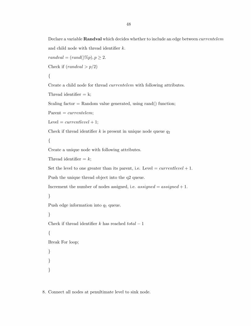
48

Declare a variable Randval which decides whether to include an edge between currentelem

and child node with thread identifier k.

randval = (rand()%p), p ≥ 2.

Check if (randval > p/2)

{

Create a child node for thread currentelem with following attributes.

Thread identifier = k;

Scaling factor = Random value generated, using rand() function;

Parent = currentelem;

Level = currentlevel + 1;

Check if thread identifier k is present in unique node queue q2

{

Create a unique node with following attributes.

Thread identifier = k;

Set the level to one greater than its parent, i.e. Level = currentlevel + 1.

Push the unique thread object into the q2 queue.

Increment the number of nodes assigned, i.e. assigned = assigned+ 1.

}

Push edge information into q1 queue.

}

Check if thread identifier k has reached total − 1

{

Break For loop;

}

}

}

8. Connect all nodes at penultimate level to sink node.

49

(a) The level of the last element in queue is the penultimate level, or lastlevel.

(b) Determine the number of elements at penultimate level, Numelements.

(c) Penultimate level elements are stored in array arr with size Numelements.

(d) Connect all elements in array arr to the sink node.

6.2.1 Forming Adjacency Matrix

We represent the random graph by an adjacency matrix. Declare an adjacency matrixAdjacencymat

with size equal to total number of application threads. Read from the queue q1 and form the

adjacency matrix created for the application.

While q1 is not empty, loop the following

{

Remove the thread object at head of queue with following attributes.

Thread identifier tid, Scale factor scalefac, Node’s parent parent.

Store Scaling factor at the location matrix location, Adjacencymat [parent][tid] = Scalefac;

}

6.3 Adding edges between Non-Adjacent levels

Step 1: Figure out the last level in the application thread control flow graph.

Step 2: Run a loop from lev = 0tolev = lastlevel−2. Within the body of the loop, collect all

elements at level lev in array arr1. Collect all thread elements at level lev + 2 in array

arr2.

Step 3: Let numelements denote the number of elements in arr1. Let numelements1 be the

number of elements in arr2. Now traverse each thread tid in arr1 and generate a random

number randval = (rand()%t), t ≥ 4, which yields a value between 0 and t−1. Randval

decides if there will be a connection from thread tid to any thread at level lev + 2.

50

Step 4: Generate index of the element to be connected in arr2. Check if randval >= t/2. If

condition holds, randomly generate index = rand()%numelements1.

Step 5: tid1 = arr2 [index] would return the thread identifier at position index in arr2.

Connect the threads tid and tid1 by an edge.

6.3.1 Necessary Condition on Outgoing Edges

Since we generate the nodes and edges connecting a node with its children randomly, there is

a possibility to create dangling nodes which have no outgoing edges. Here is a procedure to

ensure at least one outgoing edge exists for all nodes except for the sink.s

1. After finishing the two step process of random graph generation, the final step is to track

nodes which have no outgoing edges. This is accomplished by maintaining a Boolean

array visited with number of entries equal to the total number of threads in the appli-

cation, i.e. total. All entries in the visited array are initialized to 0. Threads with no

outgoing edges, except the sink node have their corresponding entries in the visited array

set to 1.

2. Figure out the level at which a dangling node exists and denote the level as curlevel.

Designate the thread identifier as tid. We need to connect tid to some arbitrary node at

the next level, i.e. curlevel + 1.

3. Let numelements be the number of elements at level curlevel + 1. Store these thread

elements in array arr1. Randomly generate a value for index = rand()%numelements.

tid1 = arr1[index] returns thread identifier present at index in array arr1. Connect the

edge between threads tid and tid1. In this way, we ensure that every thread identifier at

a level level has at least one outgoing edge.

51

CHAPTER 7. Simulation Framework and Experimental Results

This chapter outlines the components of the scheduler framework, and describes the exper-

imental setup and evaluation infrastructure. This chapter also presents the methodology to

generate morphism tables which serves as an essential input for the polymorphic thread sched-

uler. The subsequent sections in the chapter elaborate on the experiments conducted and

summarize key results. The benefits obtained by using User Satisfaction as the objective func-

tion and the performance enhancements using the novel thread scheduler are demonstrated

clearly using the result graphs. The advantages of the proposed greedy thread scheduling al-

gorithm are demonstrated by comparison against conventional thread scheduling approaches

like First Come First Serve (FCFS) and priority scheduling schemes. The chapter ends with

conclusions and scope for future work.

7.1 Simulation Framework

Extensive simulations have been conducted to evaluate the performance of the proposed user-

satisfaction based allocation scheme for heterogeneous class of applications. In our sched-

uler framework, the common performance metric across all the multithreaded applications is

throughput. For many embedded system applications such as movie players, streaming video,

video chatting, frame rate is a parameter which clearly captures user experience. Hence,

throughput generally expressed in terms of frames/sec is used as the discrete parameter in

the sigmoid function, which models user satisfaction. The following section describes the com-

ponents of the polymorphic thread scheduler framework. Figure 7.1 presents the simulation

framework for the polymorphic embedded systems scheduler in finer detail. An embedded

system simulator has been developed and implemented. A ready queue data structure is main-

52

tained, which keeps track of threads from multiple applications which are ready to run at any

time instant. The threads from different applications have a random arrival pattern when they

enter the ready queue. The other input data structures to the embedded systems scheduler are

morphism tables and the random thread flow graphs corresponding to the N multithreaded

applications, which are active in the system. Depending on the application threads lined up

for execution in the ready queue, the corresponding morphism tables are loaded at run time

into memory. As mentioned in Chapter 6, random graphs serve as benchmarks to evaluate

the proposed scheduler framework, due to the absence of industry-standard benchmarks. The

scheduler has to efficiently carry out the task of morphism assignment for the threads in the

ready queue. As mentioned in Chapter 5, the scheduler adopts different greedy scheduling

heuristics, depending on the starting position in the thread morphism tables. The morphism

choices for the threads, depends on the instantaneous resource availability. A resource allo-

cation module is invoked by the scheduler to check if resource constraints hold. This module

accepts the current resource allocation for the different thread morphisms as its input. After

communication with the resource availability layer, it returns true, if resource constraints are

satisfied and false if resource violations occur. The scheduler framework’s output is the final

morphism assignment for threads in the active cut along with their individual and total user

satisfaction. The following section describes the morphism data structure and elaborates on

the algorithm classes considered for morphism table generation.

7.2 Morphism Table Generation

This section motivates the problem of constructing morphism table patterns, based on prop-

erties of commonly used algorithm classes in embedded systems. Since polymorphic scheduler

is a futuristic approach for embedded system design, no industry standard benchmarks are

available to test the proposed framework. In order to evaluate the accuracy and usefulness of

the scheduler framework, random graphs are generated which are representative of scientific

embedded domain benchmarks. Consequently, it is of paramount importance, for these ran-

dom graphs to be representative of real benchmarks. Morphism tables also form one of the

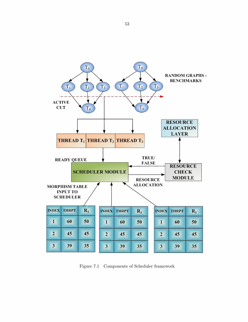
53

Figure 7.1 Components of Scheduler framework

54

essential inputs to the scheduler algorithm. As mentioned in Chapter 4, morphism table is

a scheduler data structure which stores information about thread morphisms. The entries in

the morphism table are sorted in decreasing order of their performance metric (throughput).

The columns in the morphism table are as follows. There is one column to index the different

morphism entries. The second column stores information about the throughput of a thread

morphism and the subsequent columns store details about the amount of resources required for

its execution. If the number of resource types is R, the total number of columns in a morphism

table is R + 2. The resources in the system could be the amount of Random Access Memory

(M) required, Disk Memory (D) and Processing Units (P ), which form the various columns

M,P,D in the morphism table. In the polymorphic scheduler framework, since the makeup of

applications is known only at run time, the morphism tables for the application threads are also

generated dynamically at run time. The thread morphism tables should reflect characteristics

of commonly run algorithms on embedded system. The entries in the thread morphism tables

should have variation patterns resembling the properties of an algorithm class. The number

of rows in a morphism table or thread morphisms is also decided randomly. There are five

classes of algorithms, based on which morphism table patterns are generated. When morphism

table entries adhere to an algorithm class pattern, it helps us conclusively decide which greedy

scheduling heuristic performs best, for an algorithm class. Extensive simulations using these

morphism classes and application benchmarks reveal that, the proposed polymorphic sched-

uler framework offers significant performance improvements in terms of user satisfaction over

other classical scheduling approaches. The different algorithm classes which serve as basis for

morphism table generation are as follows.

1. Matrix Manipulation class

2. Sorting Algorithm class

3. Polynomial class

4. Multiplication algorithms class

5. GCD algorithms class

55

Each algorithm class maintains the time complexities for the different thread morphisms. For

instance, the sorting class has ratios of time complexities for morphisms which realize the sort-

ing functionality. These ratios are stored in an array specific to each algorithm class. At run

time, a random number is generated which selects one among the five algorithm classes. Mor-

phism table entries are generated based on these class properties. To recall, rows in morphism

table are organized in the decreasing order of their throughputs. Hence the row entries for

thread morphism tables are generated from the bottom-upward. The number of row entries in

a thread morphism table is decided randomly. The first thread morphism or bottommost row

entry has random values generated for its throughput and resource requirements. The sub-

sequent thread morphisms are generated based on ratios within the selected algorithm class,

and values for previous row entries. The throughput for the thread morphism immediately

above the currently generated one and its corresponding resource requirements are scaled by

a ratio, randomly chosen within the algorithm class. A similar procedure is followed for gen-

erating rows all the way up to the topmost row entry in the morphism table. The following

section describes the central idea behind context size, which serves as an important metric for

performance evaluation.

7.3 Context Size

Traditional mobile phones offered support for voice-only services along with basic features in

user interface. Current day mobile phones offer extensive support for multimedia applications

along with supporting voice services. Moreover, end users expect their consumer electronic de-

vices to operate faster, in addition to offering support for a wide range of applications. Hence

it is a challenge to measure or evaluate the performance of such evolving embedded systems.

Since resource limitations are more severe in embedded systems, resource allocation plays a

crucial role in the design of an embedded system scheduler. The efficacy of the polymorphic

scheduler framework, in supporting a heterogeneous application class has to be evaluated.

Hence extreme load conditions are generated, by running several applications concurrently on

the embedded system. This includes testing the system under heavy loads and high concur-

56

rency, thereby constraining or limiting the computational resources. The goal of stress testing

the embedded system is to observe how the scheduling algorithm responds to situations, where

applications contend for limited system resources such as memory, processor cycles, network

bandwidth etc. This will present a perfect scenario for testing and evaluating the performance

of the greedy scheduler algorithm. The effectiveness of the proposed scheduler framework in

making resource allocation decisions becomes apparent only in such extreme conditions. A

good resource allocation strategy will effectively handle issues relating to resource contention

and lead to minimal performance degradations in the embedded system. When congestion oc-

curs in an embedded system, the quality of service deteriorates for applications in the system.

The typical effects of congestion include delayed response time for applications, packet loss, and

inability to accept additional applications into the system. Consequentially, any incremental

increase in computational load in the system results in drastic reductions in system throughput.

Congestion in an embedded system is analogous to the total number of applications running

concurrently along with an application. The target application is the application of interest

whose performance characteristics needs to be analyzed or observed. The target application

is randomly chosen from the currently running active set of applications. In this case, context

size refers to the total number of applications running in the system along with the target

application. In the proposed polymorphic thread scheduler, the value of the objective func-

tion (user satisfaction) is plotted against the context size. Embedded system applications are

driven by use case scenarios created by the user. Use case scenarios define the way, a sys-

tem responds to a request that originates from outside of that system. A typical use case

scenario is considered, where an embedded system user intends to run an MP3 application

along with other applications such as video, phone call etc. The end user’s interest lies in an-

alyzing the variations in user satisfaction exhibited by this application, during varying system

loads (context size). The context size in the system varies as applications leave or enter the

system, assuming the original MP3 application still keeps running. The performance of the

MP3 application can be analyzed by plotting its user satisfaction behavior for the different

57

greedy scheduling heuristics. Extensive simulations have been conducted to capture the user

satisfaction variations for a target application with increase in context size or computational

load in the system. The result graphs demonstrate that with increase in computational load,

the greedy scheduling heuristics outperform the classical thread scheduling schemes FCFS and

priority scheduling.

7.4 Experimental Results and Analysis

As mentioned in the previous section, the dynamic nature of workloads that run concurrently

along with the target application affects its performance. The extensive experiments conducted

demonstrate that the greedy scheduling heuristics adopted by the proposed scheduler, would

improve task scheduling in a multiple application, multithreaded environment. In the following

section, we discuss experimental results, where result graphs are plotted with user satisfaction

for the target application against the context size. The X-axis denotes the context size, or

number applications running concurrently along with the target application in the system.

The greedy scheduler heuristics adopted by the polymorphic scheduler traverse the morphism

table in different order. These heuristics are as follows.

1. Bottommost traversal

2. Topmost traversal

3. Top-variation traversal

4. Binary Search traversal

5. FCFS scheduling - Conventional approach

6. Priority scheduling - Conventional approach.

The experimental graphs plot user satisfaction for the target application against the total

number of applications running in the system. The target application is the application,

58

whose user satisfaction behavior is to be analyzed. The scheduling heuristics adopted by

the polymorphic thread scheduler scheme achieve greater performance benefits and resource

utilization. Therefore the proposed greedy scheduling heuristic approaches are more desirable

compared to classical scheduling schemes.

7.5 Matrix Manipulation Class

The first class of algorithms considered for generating morphism table patterns is the ma-

trix manipulation class. The time complexities for the matrix class of algorithms are O(n2),

O(n2.807) and O(n2.376) etc. The common matrix algorithms examined are matrix inversion,

determinant and matrix multiplication etc. From the results, show in Figure 7.2, we conclude

that for the matrix class of algorithms, the binary search traversal option has higher increase

in user satisfaction compared to other scheduling heuristics. The next best scheduling heuristic

for this algorithm class, is the topmost scheduling heuristic which comes close to the binary

search traversal in terms of achieving significant user satisfaction gain. This is closely followed

by the bottommost traversal approach. Overall, the bottommost scheduling heuristic suffers

the least, whereas top-variation scheduling heuristic suffers the most. From the results, we

conclude that for the matrix class of algorithms, the binary search traversal option has higher

increase in user satisfaction compared to other scheduling heuristics. Let us examine why bi-

nary scheduling heuristic performs better compared to the bottommost and other scheduling

heuristics.

For the bottommost heuristic, a case might arise, where the throughput of the thread, may not

monotonically increase with a corresponding increase in resources. Assuming one resource type,

a graph is plotted with resource type on the x-axis and throughput on the y-axis. If there is

more than one resource type, accordingly so many dimensions are present. In this graph, there

could be some regions, where a bursty increase in the throughput is experienced for increase

in resources and there may be some regions, where there is no significant throughput increase,

for increase in resources. A very good example of this kind of a behavior can be found in

59

application threads that have smaller data structures within bigger data structures. E.g. inner

structure nested within an outer structure. These application threads respond to an increase in

the cache size in the aforementioned manner. After the inner data structure fits in the cache,

the application may not show any improvement until the bigger data structure can fully fit

into the cache. Let us denote these kinds of application threads as class A. Application threads

without the bursty increase in throughput are categorized under class B. Class B threads, may

exhibit a monotonic or linear relationship between throughput and resources. When there is

a mix of both these class of application threads A and B in an active cut, the bottommost

traversal approach will allocate more resources to application threads in class B. This would

result in process starvation for applications in class A. Until the Class A application threads

reach a point, where bursty throughput appears, the bottommost scheduling heuristic keeps

allocating resources to Class B application threads. This results in an unbalanced or skewed

resource allocation among application threads, resulting in a sub-optimal solution in terms

of user satisfaction. But, this may necessarily not be the case with binary search scheduling

heuristic, since the starting position in the morphism table is at the middle morphism entries

for all threads. Since the greedy scheduling algorithm is applied from this point, it results in

a near uniform allocation state for the binary scheduling heuristic.

For illustration, consider an application which is composed of 5 threads. For the bottommost

scheduling heuristic, let the first 3 threads in the active cut be the ones that always exhibit lin-

ear increase in throughput during morphism transitions, i.e: threads which come under Class

B category. Meanwhile, let the morphism entries for the remaining 2 threads experience bursty

throughput increase in certain regions and let other regions, exhibit a non-monotonic increase

in their throughput per unit resource, similar to Class A threads. Let these two application

threads reach a point where there is temporarily no increase in the throughput at this instant.

In such a case, the bottommost scheduling heuristic always allocates more resources for the first

3 threads compared to the other 2 threads, where the throughput increase per unit resource

value is considerably low. Due to tight bounds on the amount of resources, this could result in

60

a very skewed/unbalanced allocation of resources, resulting in local maxima. In such cases, the

binary search heuristic performs better than the bottommost approach. The heuristic initially

allocates resources uniformly for all 5 threads which constitute an application. This is because

the starting position is at the middle entry in the morphism table, which can yield an optimal

solution without getting stuck at the local maxima. Since the bottommost approach decides

on its scheduling options too early in such cases, it prevents it from finding the best overall

solution.

Coming to the comparison approaches for the matrix manipulation class, FCFS scheduling out-

performs priority scheduling as shown in Figure 7.2. It is to be noted that, priority scheduling

performs badly for tasks whose run-time behavior deviates significantly from its expected or

design time behavior. Moreover the behavior of these tasks may vary with respect to time and

the number of tasks in the system. Another drawback in priority scheduling is that there is no

foolproof mechanism for mapping task requirements into priority values. In many cases, the

system designer accomplishes this mapping based on a pre-determined set of facts. Priority

scheduling performs badly in cases where, applications with low priority have higher marginal

user satisfaction increase, compared to applications with higher priority. Moreover, there may

be cases where applications with higher priority could potentially block all lower priority tasks

indefinitely from executing. If the target application chosen is one among these lower priority

tasks, it is very likely that its user satisfaction value would undergo a significant reduction

because of process starving.

7.6 Sorting class of Algorithms

The second class of algorithms considered for generating morphism table patterns is the sorting

class of algorithms. The complexities of the thread morphisms in the sorting class are O(n2)

and O(nlogn). Figure 7.3 plots the user satisfaction behavior for an application in the sort-

ing class against the context size, or the number of applications running concurrently in the

61

Figure 7.2 Matrix class: User Satisfaction vs Context Size

system. The performance of the greedy scheduling heuristics implemented by the polymorphic

thread scheduler is compared against conventional thread scheduling techniques. When the

congestion increases in an embedded system, QOS (Quality of Service) levels for application

are reduced drastically. In order to effectively handle such scenarios, a clever resource allo-

cation strategy is needed. The scheduling performance for a greedy scheduling heuristic is

measured by the user satisfaction reduction obtained as context size increases. For the sorting

class of algorithms, the observation is that the bottommost traversal heuristic outperforms

the other scheduling heuristics. The next best scheduling heuristic, which comes close to the

bottommost traversal in achieving significant user satisfaction gain, is the topmost scheduling

heuristic. For the scheduling heuristics under consideration, the value for the target applica-

tion’s user satisfaction is averaged over 50 iterations. The result graph in Figure 7.3 clearly

demonstrate that with increase in computational load, the greedy scheduling heuristics out-

62

perform classical thread scheduling schemes, namely FCFS and priority scheduling. During

times of congestion in the system, applications contend for system resources such as memory,

processor cycles etc. For the binary search scheduling heuristic, there is drastic reduction in

user satisfaction when the context size increases initially. With further increase in context size,

there is minimal variation in the target application’s user satisfaction for this heuristic. The

results also demonstrate that the topmost scheduling heuristic comes close to the bottommost

heuristic approach in achieving significant user satisfaction increases. This is closely followed

by the binary search and top-variation scheduling heuristics. Let us explain why bottommost

scheduling heuristic outperforms rest of the scheduling heuristics.

Figure 7.3 Sorting class: User Satisfaction vs Context Size

Let us recall the notion behind feasible set. The feasible set is computed at every intermedi-

63

ate step, which contains threads from multiple applications when they satisfy two conditions.

Condition 1 is there should be a possibility for a morphism switch. In other words, there

should be some morphism entry for the application thread, above their currently assigned

morphism in the morphism table, to which transition may occur. Once this is ensured, the

second condition is that after morphism transition, resource constraints should be satisfied.

Precedence among threads in the feasible set is decided by the metric user satisfaction gain

per unit resource. When there is a mix of class A and class B’s application threads in an

active cut, the bottom most traversal approach will allocate more resources to application

threads in class B. This results in an unbalanced or skewed resource allocation among applica-

tion threads, resulting in a sub-optimal solution in terms of user satisfaction. But the sorting

algorithm class consists of threads from class B. Hence the bottommost scheduling heuristic

outperforms the other scheduling heuristics. FCFS and priority scheduling are implemented as

comparison scheduling schemes. For the sorting class, priority scheduling outperforms FCFS

scheduling. As shown in Figure 7.3, regardless of the context size, priority scheduling outper-

forms FCFS scheduling heuristics for this algorithm class. While it may be true in some cases

that threads may enter the ready queue according to their application priorities, it might not

be necessarily true in all cases. In other words, there is no guarantee that the threads which

enter the ready queue earlier, have higher priority than the others appearing later in the queue.

In many cases, the embedded system designer accomplishes the mapping between problem

constraints into priority values, based on pre-determined set of facts. The priority values for

applications are derived after analyzing the past behavior of applications run in embedded

systems. More often than not, end users run a set of applications in an embedded system

regularly. In general, past application behavior provides a reasonable estimate in predicting

its future characteristics. Since the priority values for applications are based on established

set of facts, intuitively priority scheduling performs better than FCFS scheduling. On the

other hand, FCFS scheduling does not take an application’s past performance into account

and relies on the thread ordering in the ready queue to accomplish scheduling. If the target

64

application is one which requires more user interaction, then FCFS scheduling might not serve

the purpose. This is because FCFS can never guarantee a good response time for interactive

tasks and hence is not useful for scheduling interactive processes. Also, in FCFS application

threads are dispatched for execution depending on their arrival time into the ready queue.

This can result in cases, where higher priority or interactive applications may be made to wait

for lower priority applications to complete execution. This is the primary reason for priority

scheduling to outperform the FCFS scheduling strategy in the sorting algorithm class.

7.7 Polynomial Manipulation Class

The algorithm class considered for pattern generation in morphism tables is finding the GCD

for two polynomials of degree n, with fixed-size polynomial coefficients. The time complexi-

ties of the thread morphisms in this class O(n2) and O(n(logn)2log logn). Figure 7.4 plots

the user satisfaction behavior for a target application in the polynomial manipulation class

against the context size. The general observation from these graphs is that even though bi-

nary search traversal approach performs better when the context size is less, it is affected by

performance degradations as context size increases. The bottommost traversal approach also

undergoes reductions in user satisfaction and stabilizes with increase in context size. Over-

all from these results, we can conclude that for this algorithm class, the bottommost traversal

heuristic has higher increase in user satisfaction compared to the other approaches. Intuitively,

one can infer that for all the experiments conducted, as the context size increases, there are

user satisfaction reductions for all the scheduling heuristics. Similar to the sorting class, the

bottommost scheduling heuristic performs better than the binary search scheduling heuristic.

When there is a mix of class A and class B’s application threads in an active cut, the bottom

most traversal approach will allocate more resources to application threads in class B. This

results in an unbalanced or skewed resource allocation among application threads, resulting

in a sub-optimal solution in terms of user satisfaction. But the polynomial algorithm class

consists of threads only from class B. Hence the bottommost scheduling heuristic outperforms

the other scheduling heuristics. The next best scheduling heuristic which comes close to the

65

bottommost traversal in achieving significant user satisfaction gain is the binary search schedul-

ing heuristic, closely followed by topmost and top-variation scheduling schemes. Coming to

the comparison approaches for the polynomial manipulation class, FCFS scheduling scheme

performs better than the priority scheduling scheme because of the following reason. It is to

be noted that, priority scheduling performs badly for tasks whose run-time behavior deviates

significantly from its expected or design time behavior. Moreover the behavior of these tasks

may vary with respect to time and the number of tasks in the system. Another drawback

in priority scheduling is that there is no foolproof mechanism for mapping task requirements

into priority values. In many cases, the system designer accomplishes this mapping based on

a pre-determined set of facts. Priority scheduling performs badly in cases where, applications

with lower priority have higher marginal user satisfaction increase, compared to applications

with relatively higher priority. Moreover, there may be cases where applications with higher

priority could potentially block all lower priority tasks indefinitely from executing. If the tar-

get application chosen is one among these lower priority tasks, it is very likely that its user

satisfaction value would undergo a significant reduction because of process starving. Hence

FCFS scheduling offers better user satisfaction gain compared to priority scheduling as shown

in Figure 7.4.

7.8 Multiplication Class of Algorithms

The time complexities for the multiplication class morphisms are generally O(n2), O(n1.585)

and O(n1.465) etc. The result graphs for the multiplication class of algorithm plot the user

satisfaction behavior for the target application against the context size (total number of appli-

cations concurrently running along with target application), as shown in Figure 7.5. Similar

to the sorting and polynomial classes, even here the bottommost scheduling heuristic per-

forms better than the other scheduling heuristics. Overall the results conclusively demonstrate

that the bottommost scheduling heuristic performs better than the other scheduling heuris-

tics, similar to sorting and polynomial classes. As mentioned earlier in the polynomial class,

when there is a mix of class A and class B’s application threads in an active cut, the bottom

66

Figure 7.4 Polynomial class: User Satisfaction vs Context Size

most traversal approach will allocate more resources to application threads in class B. This

results in an unbalanced or skewed resource allocation among application threads, resulting

in a sub-optimal solution in terms of user satisfaction. But the multiplication algorithm class

consists of threads from class B. Hence the bottommost scheduling heuristic outperforms the

other scheduling heuristics. Another observation for the multiplication class of algorithms is

that as context size increases, applications contend for resources. When resource contention

increases, the classical scheduling approaches like FCFS and priority scheduling undergo dras-

tic performance degradations, but the greedy scheduler heuristics like are least affected by

the resource contention. This is because all these scheduler heuristics effectively implement

admission control in two phases. First phase admits resource requests into the system and

67

the second phase does resource allocation, for the admitted requests. The proposed greedy

scheduling algorithm performs better than the classical thread scheduling approaches. This

is because, when resource violations occur, the greedy scheduling heuristic approaches accept

threads into the ready queue in the decreasing order of their user satisfaction. In other words,

threads which yield higher user satisfaction increase are serviced before threads which give rise

to lesser user satisfaction increase. In FCFS scheduling, threads are scheduled based on their

order of occurrence in ready queue. In priority scheduling, threads are scheduled depending

on statically assigned application priorities. Hence, the greedy scheduling approach is more

effective in enhancing user satisfaction compared to the conventional scheduling strategies. In

FCFS, if due to resource constraints all threads in ready queue cannot be scheduled, threads

are admitted into the system, depending on their order of occurrence in the ready queue.

In the case of priority scheduling, admission control is implemented depending on statically

assigned application priorities. Coming to the comparison approaches, the FCFS scheduling

strategy outperforms the priority scheduling scheme. Due to similar reasons mentioned under

the polynomial algorithm class, FCFS scheduling performs better than priority scheduling.

7.9 GCD Class of Algorithms

This class is about finding the Greatest Common Divisor (GCD) for two n digit numbers. The

time complexities for the GCD class morphisms are O(n2) and O( n2

logn). As before, the result

graphs shown in Figure 7.6, plot the variations in user satisfaction for the target application

with increase in congestion(total number of applications concurrently running along with target

application). Similar to the sorting and polynomial classes, even in this class the bottommost

scheduling heuristic performs better than the other scheduling heuristics. Another observation

for the GCD class of algorithms is that, as context size increases, applications contend for

resources. When resource contention increases, the classical scheduling approaches like FCFS

and priority scheduling undergo drastic performance degradations, but the greedy scheduler

heuristics suffer the least due to the resource contention. Overall from the graphs we observe

that similar to the polynomial, multiplication and sorting classes, the bottommost scheduling

68

Figure 7.5 Multiplication class: User Satisfaction vs Context Size

heuristic performs better than the other scheduling heuristics. As mentioned earlier in the

polynomial and multiplication classes, when there is a mix of class A and class B’s application

threads in an active cut, the bottommost traversal approach will allocate more resources to

application threads in class B. This results in an unbalanced or skewed resource allocation

among application threads, resulting in a sub-optimal solution in terms of user satisfaction. But

the GCD algorithm class consists of threads from class B. Hence the bottommost scheduling

heuristic outperforms the other scheduling heuristics. Coming to the comparison approaches,

priority scheduling performs better than FCFS scheduling. In general, the embedded system

designer accomplishes the mapping between problem constraints into priority values, based on

well established set of facts. Since priority values for applications are derived after analyzing

their past behavior in embedded systems, it provides a reasonable estimate in predicting its

69

future characteristics. Moreover, priority values for applications are based on established set

of facts, intuitively priority scheduling performs better than FCFS scheduling. On the other

hand, FCFS scheduling does not take an application’s past performance into account and relies

on the thread ordering in the ready queue to accomplish scheduling.

Figure 7.6 GCD class: User Satisfaction vs Context Size

7.10 Analysis- Performance Overhead

The performance overhead of the proposed greedy scheduling heuristics compared to the clas-

sical scheduling approaches needs to be quantified. Hence result graphs are plotted with

execution time of the greedy scheduler heuristics on the Y-axis and context size along X-axis,

for every algorithm class. These applications are run on a processor with 3.791 GHz Proces-

sor clock frequency. The execution time of these scheduler heuristics is measured in terms of

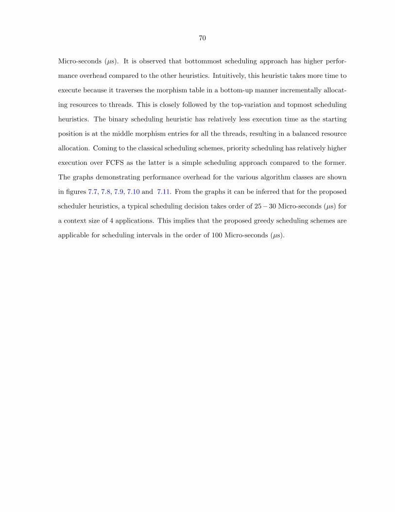
70

Micro-seconds (µs). It is observed that bottommost scheduling approach has higher perfor-

mance overhead compared to the other heuristics. Intuitively, this heuristic takes more time to

execute because it traverses the morphism table in a bottom-up manner incrementally allocat-

ing resources to threads. This is closely followed by the top-variation and topmost scheduling

heuristics. The binary scheduling heuristic has relatively less execution time as the starting

position is at the middle morphism entries for all the threads, resulting in a balanced resource

allocation. Coming to the classical scheduling schemes, priority scheduling has relatively higher

execution over FCFS as the latter is a simple scheduling approach compared to the former.

The graphs demonstrating performance overhead for the various algorithm classes are shown

in figures 7.7, 7.8, 7.9, 7.10 and 7.11. From the graphs it can be inferred that for the proposed

scheduler heuristics, a typical scheduling decision takes order of 25−30 Micro-seconds (µs) for

a context size of 4 applications. This implies that the proposed greedy scheduling schemes are

applicable for scheduling intervals in the order of 100 Micro-seconds (µs).

71

Figure 7.7 Sorting class: Execution Time vs Context Size

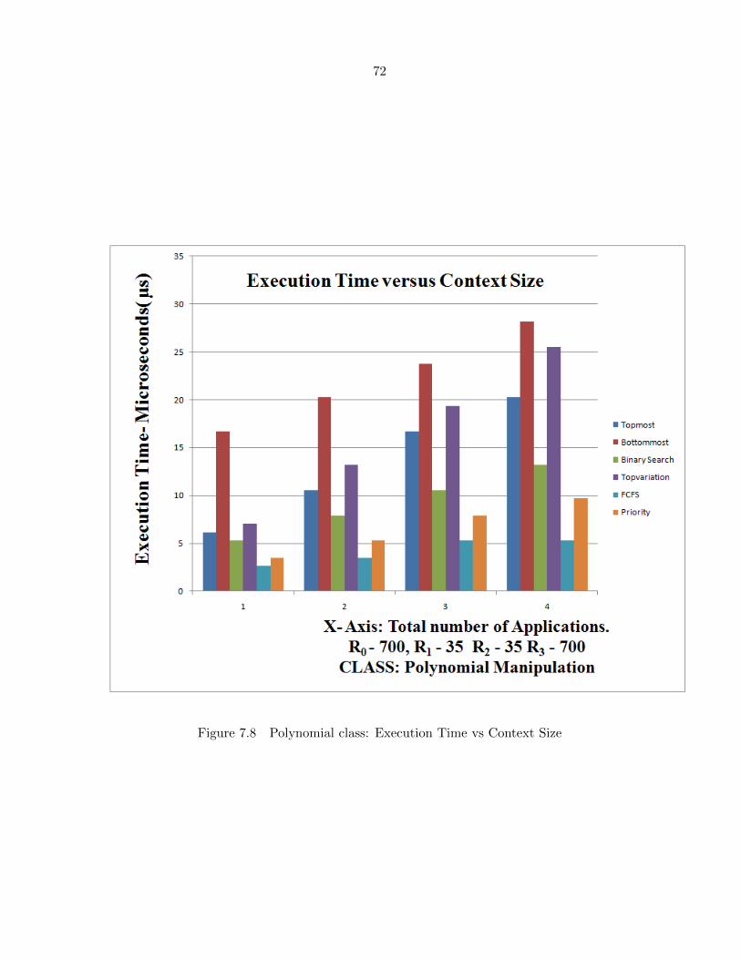
72

Figure 7.8 Polynomial class: Execution Time vs Context Size

73

Figure 7.9 Multiplication class: Execution Time vs Context Size

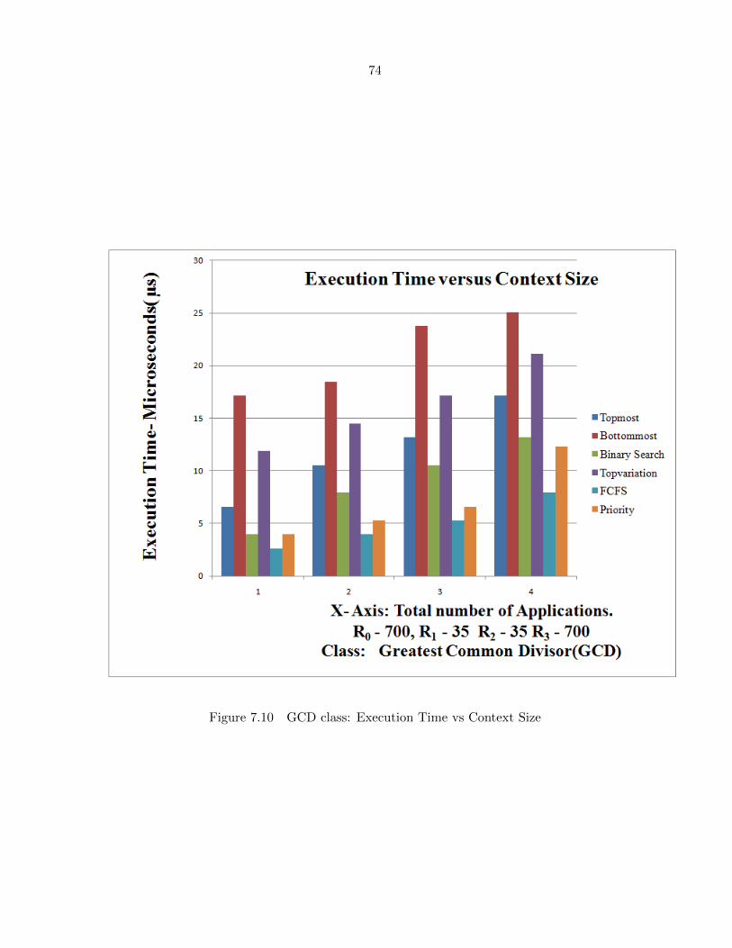
74

Figure 7.10 GCD class: Execution Time vs Context Size

75

Figure 7.11 Matrix class: Execution Time vs Context Size

76

CHAPTER 8. Conclusion

This thesis proposes a futuristic approach for embedded system scheduler design, which offers

extensive support to embedded system architects and designers. This is a pioneering attempt

at designing a novel thread scheduler for a polymorphic embedded system. In summary, a

dynamic thread scheduler which effectively operates in a multiple application, multithreaded

framework has been implemented and evaluated. Polymorphic embedded systems help in

exploring bigger design spaces compared to conventional systems like Hybrid Reconfigurable

Systems (HRS), where the design space is limited. In the proposed scheduler framework, user

satisfaction is used as the objective as opposed to conventional systems, where the performance

measure is power, energy etc. In any typical embedded system, user perception plays a key

role as it is a clear indicator of an application’s performance. Sigmoid function, an S-shaped

knee curve with near-linear central response and saturating limits, is employed to capture user

perception. The polymorphic scheduler uses the marginal utility approach to resolve resource

contention, with the intent of maximizing the objective function, which is user satisfaction. In

order to evaluate the performance of the proposed polymorphic thread scheduler framework

random graphs are used. These random graphs evaluate the efficacy of the proposed framework.

Using a set of benchmarks, which are representative of general purpose embedded applications,

we demonstrate the performance benefits of the proposed scheduler over classical scheduling

schemes like FCFS and priority scheduling. The conclusions derived from the experimental

results are stated as follows.

1. The greedy scheduling heuristics adopted by the proposed polymorphic thread scheduler

guarantees significant user satisfaction enhancements over classical thread scheduling

schemes namely FCFS and priority scheduling.

77

2. As the context size (congestion) increases, the user-satisfaction based resource allocation

strategy employed by the scheduler framework, effectively makes resource allocations,

leading to minimal performance degradations even under such extreme conditions, com-

pared to conventional thread scheduling schemes.

3. For application threads, where the increase in throughput with resources exhibits a uni-

form or monotonic relationship, bottommost scheduling heuristic gives the near-optimal

solution.

4. For application threads, where the increase in throughput with resources exhibits a non-

uniform or non-monotonic relationship, the binary search scheduling heuristic gives the

near-optimal solution.

5. Among the greedy scheduling heuristics presented, the bottommost scheduling heuristic

outperforms the other scheduling heuristics for the sorting, polynomial, GCD computa-

tion and multiplication classes. The binary scheduling heuristic performs better than the

other scheduling heuristics for the matrix algorithms class.

The proposed scheduling framework offers scope for future extensions. Currently the polymor-

phic embedded system considers several functionally equivalent software implementation alter-

natives for a thread. Future research activities could extend the proposed scheduler framework

to accommodate a much broader morphism space, offering support for hardware morphisms

as well. Also, any future work extending the proposed framework might want to explore a

broader algorithm class to generate morphism table patterns.

78

BIBLIOGRAPHY

C.L.Liu and J.W.Layland. Scheduling Algorithms for Multiprogramming in a Hard-Real-Time-

Environment Journal of ACM, Vol.20, January 1973 Pages 46-61.

J.Lehoczky, L.Sha et Al. The Rate Monotonic Scheduling Algorithm: Exact Characterization

and Average Case Behavior Proceedings of IEEE Real Time Symposium Santa Monica, CA,

December 1989 Pages 166-171.

A.K.Mok. Fundamental Design Problems of Distributed Systems for the Hard Real-Time En-

vironment Ph.D. Thesis, MIT, Dept of EE and CS. MIT/LCS/TR-297, May 1983

M.Spuri and G.Buttazo Efficient Aperiodic Service Under the Earliest Deadline Scheduling

Proceedings of 15’th IEEE Real-Time Systems Symposium, December 1994, Pages 2-11

J.Leung and J.Whitehead On the Complexity of fixed-priority scheduling of periodic, real-time

tasks. Performance Evaluation, Volume 2, Pages 237-50

M.Spuri and G.Buttazo Robust Aperiodic Scheduling Under Dynamic Priority Systems. Pro-

ceedings of 16’th IEEE Real-Time Systems Symposium, December 1995, Pages 288-299

VxWorks Programmer’s Guide VxWorks Operating System WindRiver System Inc, 1997.

QNX Operating System System Architecture and Neutrino System Architecture Guide QNX

Software Systems Ltd, 1999

David Andrews, Wesley Peck, Jason Agron Et Al. Hthreads: A Hardware/Software Co-

Designed Multithreaded RTOS Kernel 10’th International Conference on Emerging Tech-

nologies and Factory Automation(ETFA)-2005. Pages 1-4

79

Peck.W, Anderson.E, Agron.J Et Al. Hthreads: A computational model for Reconfigurable

Devices International Conference on Field Programmable Logic and Applications(FPL) 2006

Pages 1-4

D.Andrews, D.Niehaus and P.Ashenden Programming Models for Hybrid FPGA/CPU com-

putational components IEEE Computer 2004 Pages 118-120

Jason Agron, Wesley Peck, Erik Anderson, David Andrews et Al. Run-time Services for Hybrid

CPU/FPGA Systems on Chip 27’th International IEEE Real-Time Systems Symposium 2006

Pages 3-12.

V.Nollet,P.Coene,D.Verkest et Al. Desiging an Operating System for a Heterogeneous Recon-

figurable SOC. Parallel and Distributed Processing Symposium 2003 Pages 22-26.

J.Y.Mignolet, V.Nollet,P.Coene et Al. Infrastructure for design and management of relocat-

able tasks in a heterogeneous reconfigurable SOC. Design, Automation and Test in Europe

Conference and Exhibition 2003 Pages 986-991.

V.Nollet, P.Avasare, H.Eeckhaut, et Al. Run-time management of a mpsoc containing fpga

fabric tiles. IEEE Transactions on Very Large Scale Integration(VLSI) Systems, 2008. Pages

24-33, Vol.16

Pellizoni R, and Caccamo M. Real-Time Management of Hardware and Software Tasks for

FPGA-Based Embedded Systems. IEEE Computer Transactions Pages 16661680, 2007.

Nicholas Enderle and Xavier Lagrange (2003). User Satisfaction Models and Scheduling Al-

gorithms for Packet Switched Services in UMTS. Vehicular Technology Conference, VTC

Pages: 1704-1709, Vol.3

Pal S,Das S.K, Chatterjee M(2005). User Satisfaction Based Differential Services for Wireless

Data Networks ICC 2005, IEEE International Conference on Communications Pages: 1174-

1178,Vol.2

80

Ahmad I, Kamruzzaman J. and Aswatanarayaniah, S. An Improved Preemption Policy for

higher User Satisfaction International Conference on Advanced Information Networking and

Applications(AINA) 2005 Pages: 749-754,Vol.1

Dongmei Zhao, Xuemin Shen and Mark J.W Radio Resource Management for Cellular

CDMA Systems supporting Heterogeneous Services IEEE Transactions on Mobile Com-

puting, November 2002 Pages: 147-160, Vol.2

Liang Xu, Xuemin Shen and Mark J.W. Dynamic Bandwidth Allocation with Fair Scheduling

for WCDMA Systems IEEE Wireless Communications, April 2002 Pages 26-32, Vol.9

Sourav Pal,Mainak Chatterjee and Sajal K. Das. A Two-level Resource Management Scheme

in Wireless Networks Based on User Satisfaction Mobile Computing and Communications

Review, 2005 Pages 4-14, Vol.9

Sampath A. and Sarath Kumar. P, Holtzman J.M Power Control and Resource Manage-

ment for a Multimedia CDMA Wireless System IEEE International Symposium on Per-

sonal,Indoor,Mobile Radio Communications 1995 Pages 21-25, Vol. 1

Stamoulis G.D and Kalopsikakis. D, Kyrikoglou, A Efficient agent-based negotiation for

telecommunication services Global Telecommunications Conference, 1999 Pages 1989-1996,

Vol. 3

M.Xiao, Shroff N.B and Chong, E.K.P Utility-Based power control in cellular wireless systems.

INFOCOMM Conference of IEEE Computer and Communication Society 2001 Pages 412-

421, Vol.1