A Novel LMMSE Based Optimized Perez-Vega Zamanillo

Progress In Electromagnetics Research B, Vol. 63, 17–33, 2015

A Novel LMMSE Based Optimized Perez-Vega ZamanilloPropagation Path Loss Model in UHF/VHF Bands for India

Sridhar Bolli* and Mohammed Z. A. Khan

Abstract—Cognitive radio is the enabling technology for license-exempt access to the TV WhiteSpaces (TVWS). There is ever increasing demand of users in the broadcasting and communicationservices. Large portions of unused spectrum in the UHF/VHF bands exist in India which can be usedon geographical basis. This paper describes a study on path loss variation in UHF/VHF bands in India.The aim of this study is to develop and optimize a path loss model based on Linear minimum meansquare error estimation (LMMSE) for India. We propose the LMMSE based Optimized Perez-VegaZamanillo propagation path loss model. The measured path loss values, collected across India, arecompared with proposed Optimized Perez-Vega Zamanillo path loss model and other existing path lossmodels. It is found that Optimized Perez-Vega Zamanillo propagation path loss model has the leastroot mean square Error (RMSE) of 13.98 dB. Other existing path loss models have root mean squareError(RMSE) value greater than 24 dB. Therefore, Optimized Perez-Vega Zamanillo propagation pathloss model is best suited for predicting coverage area, interference analysis in India for TVWS.

1. INTRODUCTION

Cognitive radio identifies other radios in the environments that might use the same spectral resourcesand then designs a transmission methodology that minimises interference to and from other radios.It is necessary to understand the propagation channel for the identification, design, implementationand analysis of transmission methodologies. Propagation channel determines how much power emittedby transmitter is received at the receiver and also the amount of interference created at the receiver.All communication services seek frequency bands below 3.5 GHz because these frequency bands havelower propagation loss. Therefore UHF/VHF bands are ideal candidates for setting up cognitive radios.Today most of the UHF/VHF bands are used by broadcast television. The U.S. regulatory body, theFederal Communications Commission, has recently adopted rules to allow unlicensed radio transmittersto operate in the broadcast television spectrum at locations where the spectrum is not being used bythe licensed services [1]. The unused TV spectrum is often termed “white spaces”. In order to utilisethese “white spaces”, we need accurate channel models.

Path loss measurements and model comparison have been done in different parts of India [2–8].In [2] field strength measurements were conducted for VHF and UHF bands at different base stationantenna heights in the Coastal South India. These measured values were compared with differentprediction methods of Hata, ITU-R, Blomquist and Ladell, Egli, Ibrahim and Parsons. It was foundthat in sub-urban and urban regions Hata’s method gave moderate agreement with the observed values.Mobile train radio measurements for UHF band in Northern India were presented in [3]. Comparisonof three path loss models with measured data was presented in [3]. It was found that uniform theory ofdiffraction (UTD) gives good agreement in the urban zone, and over all Hata’s model shows reasonableagreement in all the environmental zones. However, the study was restricted only to Northern India.

Received 19 April 2015, Accepted 25 May 2015, Scheduled 31 May 2015* Corresponding author: Sridhar Bolli ([email protected]).The authors are with the Department of Electrical Engineering, IIT Hyderabad, India.

18 Bolli and Khan

In [4] mobile train measurements were conducted in the UHF band in Western India. Measured pathloss values were compared with seven path loss models using standard deviation to show that Walfishand Bertoni’s method gave good agreement followed by Hata. Investigation of attenuation of VHFsignals in band I and band II for Chennai TV and FM stations has been done in [5]. The experimentaldata collected in a RF survey from Chennai TV and FM stations have been utilized to deduce path lossexponents and these have been compared with the exponents deduced from the Perez-Vega Zamanillomodel. Path loss analysis using Pervez-Vega Zamanillo model in Indian subcontinent for UHF/VHFbands was presented in [6]. Experimental data were collected on signal measurements at 19 placesin India, and all these experimental carrier levels of the signal originating from various transmitterswere monitored at different distances, the signals levels were averaged and then converted into pathloss values. These observed path loss values were converted into path loss exponents. These werecompared with the model predicted values following the approach of Perez-Vega and Zamanillo. In [7]comparison of different path loss propagation models with measured field data was done in plane areain northern region of India, i.e., border district of Punjab and Jammu. It was found that Cost-231model is best suited for plane area in northern region of the border district of Punjab (India). Path lossmodels for broadcasting applications namely free space, Okumara, Okumara Hata, Extension of Hata,Hata-Davidson Model and Extended COST-231 Hata models were compared with path loss measured inbordering area of Punjab (State: India) and bordering area of Jammu (State: India) at different powersand antenna heights of broadcasting station [8]. A common fixed numerical value was then calculatedseparately for each model after taking average MSE of the respective model. The fixed numerical value,found for each model was then added to the respective model formula to get a new modified formula.Modified models were found to be best fitted for 100 W and 10 KW FM stations.

In other countries like USA, Longley-Rice Irregular Terrain model (ITM) has shown goodperformance in predicting TVWS in Seattle, WA [9]. Therefore, we have used Longley-Rice IrregularTerrain model(ITM) to compare with the measured path loss data collected at different places in India.In [10] Field strength measurements were conducted along six routes that spanned urban, suburban andrural areas of Kwara State, Nigeria. Measurement results were then compared with pathloss predictionof eight widely used empirical models. Least squares and linear iterative methods are employed tooptimise HataDavidson’s model, as it showed best fit compared with other models. Propagation modelsfor forest environments of Nigeria at the VHF and UHF bands are examined in [11]. The results of thepaper [11] show that the ITU-R foliage attenuation model is not suitable to predict the propagationloss between the radio transmitter with height of 130 m and the receiver located near the forest ground.In [11] it was found that free space model (which considers only the direct ray) augmented by theappropriate vegetation loss is more accurate than the other models.

There are many path loss models in VHF/UHF bands as discussed in Section 2 of our paper. So,we wanted to find the best path loss model among all of these path loss models. India has many cities,with different terrain and sizes. Also, some cities are well developed and some cities are in developingstages. So, we have selected many cities for our study on path loss variation in various parts of India.In this paper, we have measured and collected the carrier signal level, from Doordarshan (DD) TVtransmitters located in New Delhi, Mumbai, Hyderabad and Chennai. Table 1 shows details of DD TVtransmitters situated in Hyderabad, Chennai, New Delhi and Mumbai. In addition, the measurementdata given in [6], was also used. We select the Perez-Vega Zamanillo path loss model, for optimizationusing Linear minimum mean square error estimation (LMMSE) because Perez-Vega Zamanillo modelshowed good performance when compared to other known path loss models [12]. The performance of thisOptimized model was compared with other propagation path loss models. Measured path loss values

Table 1. List of transmitters in India from where data was collected.

Location of Tx Tx Height (m) Tx Frequency (MHz)Hyderabad 150 62.25, 224.25Chennai 175 175.23, 189.26

New Delhi 235 175.25, 189.25Mumbai 300 182.25, 224.25

Progress In Electromagnetics Research B, Vol. 63, 2015 19

were compared with predicted values from Optimized Perez-Vega Zamanillo, Perez-Vega Zamanillo,Longley-Rice, Hata, Egli, COST 231, Walfisch and Ikegami, Walfisch and Bertoni, ITU-R P.529-3,Green-Obaidat and FSPL models. It is found that Optimized Perez-Vega Zamanillo model is the bestsince it has the least Root Mean Square Error (RMSE) among the existing path loss models.

This paper is organised as follows: Section 1 provides introduction. Section 2 describes propagationmodels used for comparison. Section 3 provides the method of data collection. Section 4 describes theLMMSE Based optimization process. Section 5 gives plots comparing measured path loss and path losspredicted by various models. Section 6 gives the conclusion.

2. RADIO PROPAGATION PATH LOSS MODEL

A radio propagation model is an empirical mathematical formulation for characterization of radio wavepropagation as a function of frequency, distance and other conditions. In this paper following 10 modelshave been considered.

2.1. Hata Model

This model was developed by Y. Okumura and M. Hata and is based on measurements in urbanand suburban areas in Japan in 1968 [13]. The Okumura-Hata model also assumes that there are nodominant obstacles between the BS and the MS, and that the terrain profile changes only slowly [14].

2.2. Egli Model

Egli model is a terrain model for radio frequency propagation. This model is applicable at frequencyfrom 40 MHz to 900 MHz. This model was developed from real-world data on UHF and VHF televisiontransmissions in several large cities. It predicts the total path loss for a point-to-point link. This modeldoes not take into account travel through some vegetative obstruction, such as trees or shrubbery [17].

2.3. Perez-Vega Zamanillo Model

Based on the FCC curves, Perez-Vega and Zamanillo developed a computational path loss model. It isa simple propagation model for the VHF and UHF bands. It allows the estimation of median path loss,received power, or electrical field strength which usually is sufficient in many practical applications. Themodel is independent of frequency and is applicable to outdoor environments in a range of distancesfrom about 0.5 mi (800 m) up to 40 mi (64.36 km) and transmitting antenna heights from 100 ft (30.48 m)up to 2000 ft (609.6 m), and is based on a receiving antenna height of 30 ft (9 m) [15].

2.4. Cost-231 Model

It is extensively used model for predicting path loss in mobile wireless system. The frequency range ofoperation of this model is 500 MHz to 2000 MHz. This model requires that the base station antenna ishigher than all adjacent rooftops [24, 25].

2.5. Walfisch-Ikegami Model

This model distinguishes between LOS and non-line-of-sight (NLOS) propagation situations. The modelconsiders only the buildings in the vertical plane between the transmitter and the receiver. Since, thereare a lot of objects in realistic areas such as buildings, houses, roads, trees and river. Also, it is verydifficult to classify these objects in the propagation path. This make the WI model prone to errors [19].

2.6. Green-Obaidat Model

Green and Obaidat developed a path loss model for wireless LANs operating at 2.4 GHz that takesantenna height into account. This model considers the path loss due to Fresnel zone with near earthantenna height (i.e., typically between 1 and 2 meters) more accurately. This model does not take intoaccount the impact of fading caused by several objects, e.g., building, foliage, etc. [21].

20 Bolli and Khan

2.7. ITU-R P.529-3 Model

This model provides curves for predicting field strength under average conditions for three frequencyranges. It also provides analytical expressions which are valid for certain frequency ranges andconditions, and various correction factors which can be used to refine the average predictions. Thematerial in the Recommendation is statistical in nature and oriented towards application to planningand system design [20].

2.8. Walfisch-Bertoni Model

This model is suited for dense urban areas in which the buildings have uniform height and separationdistances. Any building height variations causes a significant error in the prediction of this model [18].

2.9. Free Space Path loss Model (FSPL)

Free-space propagation model is used to predict received signal strength when the path between thetransmitter and the receiver is a clear and unobstructed line-of-sight [22].

2.10. Longley-Rice Model

The Longley-Rice model is a radio propagation model for predicting the attenuation of radio signals fora telecommunication link in the frequency range of 20 MHz to 20 GHz. The Longley-Rice model is alsoknown as the Irregular Terrain Model (ITM) because it takes into account the terrain elevation andirregularities,(hills, mountains, etc.). The limitation of this model is that it does not take any accountof buildings and foliage [23].

3. MEASUREMENT CAMPAIGN

This section describes the steps followed during data collection and it gives the description of theequipment used. The data collection tool is composed of Anritsu spectrum analyzer MS2713E globalpositioning system receiver set (GPS system). The height of Doordarshan (DD) TV transmitters locatedin Mumbai, New Delhi, Chennai and Hyderabad are 300 m, 235 m, 175 m and 150 m respectively. Wewanted to obtain path loss measurement data for TV transmitters which differ significantly in theirantenna heights. Therefore, we have selected these cities for data collection. Power levels of Doordarshan(DD) TV Transmitter in New Delhi, Mumbai, Hyderabad and Chennai cities were measured at differentdistances from the transmitter, using Anritsu spectrum analyzer MS2713E.

While transmission is taking place, Anritsu spectrum analyzer was placed inside a car and drivenalong the routes in Hyderabad, Chennai, Mumbai, New Delhi cities shown in Figures 1–4. Receivedpower was measured continuously and stored in an external pen drive for subsequent analysis.

From these received power levels, path loss was calculated.

Figure 1. Measurement routes in Hyderabad. Figure 2. Measurement routes in Mumbai.


Figure 3. Measurement routes in New Delhi. Figure 4. Measurement routes in Chennai.

We have used [6] to obtain path loss values of UHF/VHF transmitters located in other parts ofIndia. From [6], measured pathloss exponent values (n) for received power of transmitters located invarious parts of India were obtained. From these measured pathloss exponent values, path loss L in dBwas calculated using formula given below:

L = 10n log10(d) + L0 dB, (1)

where d is distance between TX and RX in meters and L0 is attenuation at 1 m in free space:

L0 = 20 log10

(4πλ

), (2)

where λ is wavelength of transmitted wave in meters.We have compared the measured path loss values with Perez-Vega Zamanillo, Hata, Egli, COST

231, Walfisch and Ikegami, Walfisch and Bertoni, ITU-R P.529-3, Green-Obaidat and FSPL modelsin [12]. It is found that measured path loss values are more close to Perez-Vega Zamanillo model.

4. OPTIMIZATION PROCESS

A general flow chart of optimization process used in this paper is shown in Figure 5. Note that thisprocedure was used to optimize Hata model in [16]. Measured path loss values were compared usingRMSE, with predicted values from Perez-Vega Zamanillo, Hata, Egli, COST 231, Walfisch and Ikegami,Walfisch and Bertoni, ITU-R P.529-3, Green-Obaidat and FSPL models across 20 different places inIndia [12]. Perez-Vega Zamanillo model was found to be the better suited model for India. Therefore,Perez-Vega Zamanillo model is selected for optimization in block 2 of Figure 5. We have selectedLinear minimum mean square error estimation (LMMSE) as the Optimization process. The optimisedmodel is then validated in Mumbai, New Delhi, Hyderabad, Coastal Andhra, Chennai, Muzaffarnagar,Saharanpur, Pune, Neral, Ghaziabad, Meerut, Kalyan, Vangani, Talegaon, and Tirupati. Statisticalanalysis such as Root mean square error (RMSE) was used to compare between the Optimized modeland other known models.

4.1. Optimization into the Model

In this paper, optimizing of Perez-Vega Zamanillo model is done using Linear minimum mean squareerror estimation(LMMSE). In the present study, observed path loss values at different receiving antennaheights have been corrected to 9m height using the procedure given in [15].

Let n be the total number of set of measurements consisting of Path loss (Y ) in dB at distanced meters from the transmitting antenna of height h in meters and whose frequency of transmission isf (Hz). From Perez-Vega Zamanillo model, Path loss Yi in dB is expressed as below:

Yi = Y0 + 10n log10(di) dB, (3)

22 Bolli and Khan

where Yi is the ith Measured Path loss in dB at distance di between TX and RX in meters for transmitterof height hi and whose frquency of transmission is fi. Y0 is attenuation at 1m in free space:

Y0 = 20 log10

(4πλi

), (4)

where λi is wavelength of ith transmitted wave in m. The path loss exponent is characterized as afunction of distance and transmitting antenna height. According to Perez-Vega model n is given by:

n =4∑

u=0

4∑v=0

auvhiudi

v. (5)

The values of coefficients auv are given in [15].Combining (3), (4), (5) we get:

Yi = 20 log10

(4πλi

)+ 10

4∑u=0

4∑v=0

auvhiudi

v log10(di). (6)

Equation (6) can be further simplified as:

Yi = 20 log10

(4πc

)+ 20 log fi + 10

4∑u=0

4∑v=0

auvhiudi

v log10(di). (7)

Using Table 2, above equation can be written as:

Yi = a0 +26∑

k=1

akXk. (8)

Terms a0, a1, a2, a3, . . ., a26 are all constants. Omitting subscript i for simplification, we have:

Y = a0 +26∑

k=1

akXk, (9)

Now we have a LMMSE estimator (Yl), where estimation of random variable Y is based on observationsof multiple random variables, X1, X2, X3, . . ., X26.

Table 2. Expression of random variables in Perez-Vega Zamanillo model.

Random Variable ExpressionX1 log fi

X2 h0i d

0 log di

X3 h0i d

1i log di

X4 h0i d

2i log di

X5 h0i d

3i log di

X6 h0i d

4i log di

X7 h1i d

0i log di

X8 h1i d

1i log di

X9 h1i d

2i log di

X10 h1i d

3i log di

X11 h1i d

4i log di

X12 h2i d

0i log di

X13 h2i d

1i log di

Random Variable ExpressionX14 h2

i d2i log di

X15 h2i d

3i log di

X16 h2i d

4i log di

X17 h3i d

0i log di

X18 h3i d

1i log di

X19 h3i d

2i log di

X20 h3i d

3i log di

X21 h3i d

4i log di

X22 h4i d

0i log di

X23 h4i d

1i log di

X24 h4i d

2i log di

X25 h4i d

3i log di

X26 h4i d

4i log di


The LMMSE estimator may be written in the form

Yl = y(X) = a0 +26∑

j=1

ajXj . (10)

Now we have to find coefficients ai such that mean square error is minimized, i.e.,

minai

E

⎡⎣⎛⎝Y −

⎛⎝a0 +

26∑j=1

ajXj

⎞⎠

⎞⎠

2⎤⎦ . (11)

To minimize the expression in (11), we differentiate it with respect to ai for i = 0, 1, 2, . . . , 26, and seteach of the derivatives to 0. First differentiating with respect to a0 and setting the result to 0, we have

E[Y ] = E[a0 +26∑

j=1

ajXj ] = E[Yl], (12)

=⇒ a0 = μY −L∑

j=1

ajμXj , where μY = E[Y ] and μXj = E[Xj ]. (13)

Using (13) to substitute for a0 in (10), it follows that

Yl = μY +26∑

j=1

aj

(Xj − μXj

). (14)

Using (14), mean square error criterion (11) can be rewritten as :

E[{(Y − μY ) −

(Yl − μY

)}2

]= E

⎡⎣

⎛⎝Y −

26∑j=1

(ajXj

)⎞⎠

2⎤⎦ , (15)

whereY = Y − μY , Xj = Xj − μXj . (16)

Differentiating (15) with respect to each of the remaining coefficients ai, i = 1, 2, . . . , 26, and settingthe result to zero produces the equations

E

⎡⎣⎛⎝Y −

26∑j=1

ajXj

⎞⎠ Xi

⎤⎦ = 0, i = 1, 2, . . . , 26. (17)

From (14) and (17), we have

E[(Y − Yl)Xi] = 0, i = 1, 2, . . . , 26. (18)

From (17) we haveL∑

j=1

σXiXjaj = σXiY , (19)

where σXiXj is the covariance of Xi and Xj and σXiY is the covariance of Xi and Yi. Collecting theseequations in matrix form, we obtain⎡

⎢⎢⎣σX1X1 σX1X2 · · · σX1X26

σX2X1 σX2X2 · · · σX2X26

......

. . ....

σX26X1 σX26X2 · · · σX26X26

⎤⎥⎥⎦

⎡⎢⎢⎣

a1

a2...

a26

⎤⎥⎥⎦ =

⎡⎢⎢⎣

σX1Y

σX2Y...

σX26Y

⎤⎥⎥⎦ . (20)

24 Bolli and Khan

This set of equations are referred to as the normal equations. These normal equations can be writtenin more compact matrix notation:

(CXX)A = CXY , (21)

where the definitions are evident on comparing last two equations.The solution of this set of 26 equations in 26 unknowns yields the aj for j = 1, . . . , 26, and these

values may be substituted in (14) to completely specify the estimator. In matrix notation the solutionis

A = (CXX)−1CXY . (22)

Measurement data collected for transmitters located in Mumbai, New Delhi, Hyderabad, CoastalAndhra, Ghaziabad, Meerut, Kalyan, Vangani, Talegoan, Pangoli, Karjat and Chennai, was used tocalculate σXiXj and σXiY values. These calculated σXiXj and σXiY values are substituted in (22), toget the coefficients of Optimized Perez-Vega Zamanillo Model as given below in Table 3.

Table 3. Coefficients of optimized Perez-Vega Zamanillo model.

Coefficients Value

a0 −1.316059571257524e+002

a1 10.749305655172163

a2 55.244971979911995

a3 −5.259259194608717e-004

a4 7.511798058893486e-009

a5 −1.728227920979650e-014

a6 −2.094620171015809e-019

a7 −0.838372052342023

a8 3.279221332838490e-005

a9 −5.477200369749959e-010

a10 2.792227844898064e-015

a11 3.132291099616113e-021

a12 0.010636668971601

a13 −4.145240978477376e-007

Coefficients Value

a14 7.243743776746409e-012

a15 −4.024001323345321e-017

a16 −2.279606949659275e-023

a17 −4.412139591311738e-005

a18 1.685472705671079e-009

a19 −2.919411953590148e-014

a20 1.486966165594136e-019

a21 2.349453443660299e-025

a22 5.958804483573685e-008

a23 −2.242115276950905e-012

a24 3.826254001773790e-017

a25 −1.738412909795608e-022

a26 −5.206773596529897e-028

5. COMPARISON RESULTS

In this section we present performance comparison in terms of RMSE. For uniformity the observedpath loss values at different receiving antenna heights have been corrected to 9m height using theprocedure given in [15]. We have compared measured path loss values with predicted values fromOptimized Perez-Vega Zamanillo, Perez-Vega Zamanillo, Longley-Rice, Hata, Egli, COST 231, Walfischand Ikegami, Walfisch and Bertoni, ITU-R P.529-3, Green-Obaidat and FSPL models. In Hyderabad,Chennai, Mumbai and New-Delhi cities, path loss for Longley-Rice model was calculated using Point-to-Point method. For other places, path loss for Longley-Rice model was calculated using Area Predictionmethod.

Root Mean Square Error (RMSE) was calculated between measured path loss value and thosepredicted by path loss model using

RMSE =√(∑

(Pm − Pr)2/N), (23)

wherePm: Measured Path Loss (dB)Pr: Predicted Path Loss (dB)N : Number of Measured Data Points.

Tables 4 & 5 show the RMSE obtained between measured path loss and those predicted by the pathloss models across 48 routes in India. Optimized Perez-Vega Zamanillo model is validated at different


Table 4. Comparison of RMSE for various path loss models with measured data.

Location

of

Transmitter

Transmitter

Frequency

(MHz)

Transmitter

Height

(m)

RMSE

for

Optimized

Perez-Vega

Zamanillo

(dB)

RMSE

for

Perez-Vega

Zamanillo

(dB)

RMSE

for Hata

(dB)

RMSE

for

Green

Obaidat

(dB)

RMSE

for

Walfisch

Ikegami

(dB)

RMSE

for

Walfisch

Bertoni

(dB)

Coastal

Andhra

(Urban)

150 16 3.534071 1.928734 8.617627 24.92429 24.779159 35.659767

Coastal

Andhra

(Urban)

150 30 5.00466 1.846684 8.731298 24.54734 18.929366 20.370636

Coastal

Andhra

(Urban)

150 40 8.491702 2.310596 8.617888 24.570284 16.362293 18.920772

Coastal

Andhra

(Urban)

440 30 9.715568 2.417757 4.863326 26.608021 19.222075 18.418948

Coastal

Andhra

(Urban)

440 40 11.772175 2.762024 5.229462 25.984307 16.032524 17.59117

Chennai

(route-1)175.23 175 16.1604 43.266549 32.214485 69.149439 36.088907 27.962848

Chennai

(route-2)175.23 175 12.271322 45.522951 33.956242 71.023336 38.36332 29.047682

Chennai

(route-3)175.23 175 11.754603 47.410859 36.03672 72.385147 41.201276 30.552929

Chennai

(route-4)175.23 175 13.353393 40.127996 30.053401 63.650893 37.931666 22.515824

Chennai

(route-5)175.23 175 12.025285 42.958959 33.202365 67.914384 40.184195 26.584949

Chennai

(route-1)189.26 175 14.747048 46.161976 35.675225 73.707279 38.324451 31.942417

Chennai

(route-2)189.26 175 12.911291 42.470917 30.751453 67.054919 35.600167 25.088119

Chennai

(route-3)189.26 175 10.996772 51.62265 40.356003 77.014495 44.847835 34.950577

Chennai

(route-4)189.26 175 8.965308 42.92699 32.673092 66.668522 40.137027 24.940018

Chennai

(route-5)189.26 175 10.103468 46.196329 36.266491 70.998208 42.817729 29.495679

Ghaziabad 320 30 10.550893 16.459898 22.211366 14.328105 13.845147 34.474538

Hyderabad

(route-1)62.25 150 28.785712 72.572123 59.578224 97.326394 70.944087 55.350714

Hyderabad

(route-2)62.25 150 29.251249 68.371554 58.715296 93.478383 73.920539 52.158673

26 Bolli and Khan

Location

of

Transmitter

Transmitter

Frequency

(MHz)

Transmitter

Height

(m)

RMSE

for

Optimized

Perez-Vega

Zamanillo

(dB)

RMSE

for

Perez-Vega

Zamanillo

(dB)

RMSE

for Hata

(dB)

RMSE

for

Green

Obaidat

(dB)

RMSE

for

Walfisch

Ikegami

(dB)

RMSE

for

Walfisch

Bertoni

(dB)

Hyderabad

(route-1)224.25 150 17.271673 47.446138 39.007547 73.353159 46.346816 31.884137

Hyderabad

(route-2)224.25 150 7.446961 44.902007 33.085971 69.753323 37.708881 27.213414

Hyderabad

(route-3)224.25 150 12.518862 42.333018 34.078104 67.395188 42.453747 26.231866

Kalyan 320 49 15.622345 6.156842 8.364521 27.519219 14.544003 17.162961

Kurla 320 32 26.4429 15.079199 8.02059 39.886769 21.164916 8.997678

Meerut 320 40 10.550893 16.459898 22.211366 14.328105 13.845147 34.474538

Mumbai

(route-1)182.25 300 17.682736 61.563193 46.015483 84.318475 45.88266 42.07352

Mumbai

(route-2)182.25 300 6.88652 42.913344 34.024177 65.499205 39.085761 24.888407

Mumbai

(route-1)224.25 300 12.182778 43.058666 32.064011 65.166273 33.746457 25.893359

Mumbai

(route-2)224.25 300 19.218936 56.808463 42.462367 80.324414 41.331471 38.525012

Mumbai

(route-3)224.25 300 7.894556 34.562467 27.487063 57.639087 32.337596 17.399604

Muzaffarnagar 320 40 11.023052 19.153957 23.361808 9.229004 6.821531 35.317779

Neral 320 25 9.380195 6.575476 8.031796 28.148601 18.703303 20.092804

New Delhi

(route-1)175.25 235 9.663962 53.732046 45.711076 78.549451 52.077073 37.531463

New Delhi

(route-2)175.25 235 10.490144 43.29448 37.663299 70.55457 44.088478 30.237051

New Delhi

(route-3)175.25 235 8.278358 45.916731 39.148277 71.350224 46.100547 30.61131

New Delhi

(route-1)189.25 235 9.963577 41.117641 35.342401 68.044836 41.458921 27.734652

New Delhi

(route-2)189.25 235 8.972927 40.040521 33.87377 65.499275 40.923211 24.841618

New Delhi 320 40 17.287122 9.81371 13.264309 26.422852 10.529273 22.413681

Pune 320 45 11.632418 12.088047 17.391776 19.234135 8.712402 27.717504

Saharanpur 320 40 8.996877 15.797657 19.849099 12.279645 5.595488 31.847499

Talegaon 320 115 13.706138 8.437785 8.358142 29.58864 13.723777 15.226172

Tirupati 189.25 30 16.40488 5.284888 7.284491 32.337074 11.679938 16.043294

Vangani 320 26 8.249331 10.908134 18.201671 18.72141 13.123294 30.829985

Chennai

(route-1)62.25 130 24.652164 7.871311 4.871851 27.200754 24.22061 13.621755

Chennai

(route-2)62.25 130 22.361317 6.778475 5.640416 29.094933 27.427642 11.857094


Location

of

Transmitter

Transmitter

Frequency

(MHz)

Transmitter

Height

(m)

RMSE

for

Optimized

Perez-Vega

Zamanillo

(dB)

RMSE

for

Perez-Vega

Zamanillo

(dB)

RMSE

for Hata

(dB)

RMSE

for

Green

Obaidat

(dB)

RMSE

for

Walfisch

Ikegami

(dB)

RMSE

for

Walfisch

Bertoni

(dB)

Chennai

(route-3)62.25 130 24.310852 6.631586 9.535392 29.925722 29.225285 13.598483

Chennai

(route-4)62.25 130 27.565855 11.975789 10.992581 26.82781 27.533619 17.71194

Chennai

(route-5)62.25 130 23.079392 7.933264 7.243036 27.946695 28.445512 13.660561

Chennai

(route-6)62.25 130 21.285998 6.69998 7.64971 30.482901 30.045861 11.49775

Average

RMSE

(dB)

- - 13.98788831 28.9306304 24.95804302 49.54073948 31.21697881 26.31589898

Table 5. Comparison of RMSE for various path loss models with measured data.

Location

of

Transmitter

Transmitter

Frequency

(MHz)

Transmitter

Height

(m)

RMSE for

Free Space

(dB)

RMSE for

Egli (dB)

RMSE for

Cost-231

(dB)

RMSE for

ITU-R

P.529-3

(dB)

RMSE for

Longley

Rice

(dB)

Coastal

Andhra

(Urban)

150 16 32.481693 120.932299 5.16105 8.812686 15.443014

Coastal

Andhra

(Urban)

150 30 26.584644 121.342566 5.276135 8.934519 12.464804

Coastal

Andhra

(Urban)

150 40 24.001216 121.362515 5.162812 8.833159 11.569846

Coastal

Andhra

(Urban)

440 30 31.620139 119.251826 10.46289 5.464588 18.845938

Coastal

Andhra

(Urban)

440 40 28.43764 119.904403 10.834781 5.89166 17.436528

Chennai

(route-1)175.23 175 44.454981 78.91671 34.480981 32.214485 42.593168

Chennai

(route-2)175.23 175 46.79447 76.03508 36.278288 33.956242 46.346478

Chennai

(route-3)175.23 175 49.601941 74.75169 38.354676 36.03672 48.43179

Chennai

(route-4)175.23 175 46.265179 83.156138 32.347478 30.053401 45.106953

Chennai

(route-5)175.23 175 48.618527 79.254706 35.523938 33.202365 46.361891

28 Bolli and Khan

Location

of

Transmitter

Transmitter

Frequency

(MHz)

Transmitter

Height

(m)

RMSE for

Free Space

(dB)

RMSE for

Egli (dB)

RMSE for

Cost-231

(dB)

RMSE for

ITU-R

P.529-3

(dB)

RMSE for

Longley

Rice

(dB)

Chennai

(route-1)189.26 175 47.073855 74.352359 37.453657 35.675225 45.123219

Chennai

(route-2)189.26 175 44.417506 79.660436 32.560302 30.751453 43.926262

Chennai

(route-3)189.26 175 53.610895 70.174203 42.16046 40.356003 52.565339

Chennai

(route-4)189.26 175 48.932702 79.7398 34.489771 32.673092 47.874808

Chennai

(route-5)189.26 175 51.628408 76.186965 38.074002 36.266491 48.635438

Ghaziabad 320 30 20.82504 134.585928 25.331469 22.758307 7.606284

Hyderabad

(route-1)62.25 150 74.951388 49.759445 69.07302 59.578224 63.931063

Hyderabad

(route-2)62.25 150 77.966714 53.681808 68.280178 58.635772 70.363707

Hyderabad

(route-1)224.25 150 55.843944 74.147292 38.120372 38.973798 52.643145

Hyderabad

(route-2)224.25 150 47.215411 76.504965 32.19213 33.085971 40.180846

Hyderabad

(route-3)224.25 150 51.939931 79.804414 33.194311 33.978343 49.234658

Kalyan 320 49 24.402232 118.99 10.977469 8.424396 17.590746

Kurla 320 32 31.710758 106.620855 6.738227 8.02059 27.248884

Meerut 320 40 20.82504 134.585928 25.331469 22.758307 7.606284

Mumbai

(route-1)182.25 300 54.533615 63.877614 48.089677 46.015483 54.055552

Mumbai

(route-2)182.25 300 47.768622 81.961598 36.097144 32.896392 44.209666

Mumbai

(route-1)224.25 300 43.112149 84.337111 31.21802 31.728206 40.09859

Mumbai

(route-2)224.25 300 50.695381 68.673055 41.587554 42.462367 50.184329

Mumbai

(route-3)224.25 300 41.839201 89.420866 26.602297 25.950156 37.69197

Muzaffarnagar 320 40 13.297329 137.709464 26.707089 24.492622 5.554998

Neral 320 25 28.805545 118.192959 10.693912 8.031796 20.077267

New Delhi

(route-1)175.25 235 60.583736 69.506165 48.052233 45.193729 57.786141

New Delhi

(route-2)175.25 235 52.607232 78.112397 39.991326 36.198582 45.829496

New Delhi

(route-3)175.25 235 54.622868 76.409975 41.489406 38.375249 51.361278

New Delhi

(route-1)189.25 235 50.28768 80.324094 37.141605 33.974308 44.080905


Location

of

Transmitter

Transmitter

Frequency

(MHz)

Transmitter

Height

(m)

RMSE for

Free Space

(dB)

RMSE for

Egli (dB)

RMSE for

Cost-231

(dB)

RMSE for

ITU-R

P.529-3

(dB)

RMSE for

Longley

Rice

(dB)

New Delhi

(route-2)189.25 235 49.7607 81.815966 35.685509 32.958375 46.74191

New Delhi 320 40 20.469321 122.158881 15.824168 13.264309 15.838948

Pune 320 45 16.396865 129.156962 20.480173 17.649377 8.201219

Saharanpur 320 40 15.148229 134.244973 23.212977 20.947544 4.361736

Talegaon 320 115 23.246175 117.488583 9.75684 8.31993 20.103109

Tirupati 189.25 30 20.32507 114.481924 6.297165 7.284491 16.60808

Vangani 320 26 21.277754 129.260862 21.25272 18.211985 11.940045

Chennai

(route-1)62.25 130 28.06711 118.893701 9.399013 7.663228 5.843671

Chennai

(route-2)62.25 130 31.271608 117.029331 11.929025 6.217767 5.867691

Chennai

(route-3)62.25 130 32.918977 117.12852 14.369721 7.729493 5.512854

Chennai

(route-4)62.25 130 31.141728 121.139491 13.277847 12.631406 8.35588

Chennai

(route-5)62.25 130 32.248312 118.528393 12.376877 8.486163 4.688437

Chennai

(route-6)62.25 130 33.882946 115.984028 14.203048 6.278878 6.122784

Average

RMSE

(dB)

- - 39.26067515 97.69873425 27.15823358 24.96453402 31.04682602

Figure 5. Flow chart of optimization process.

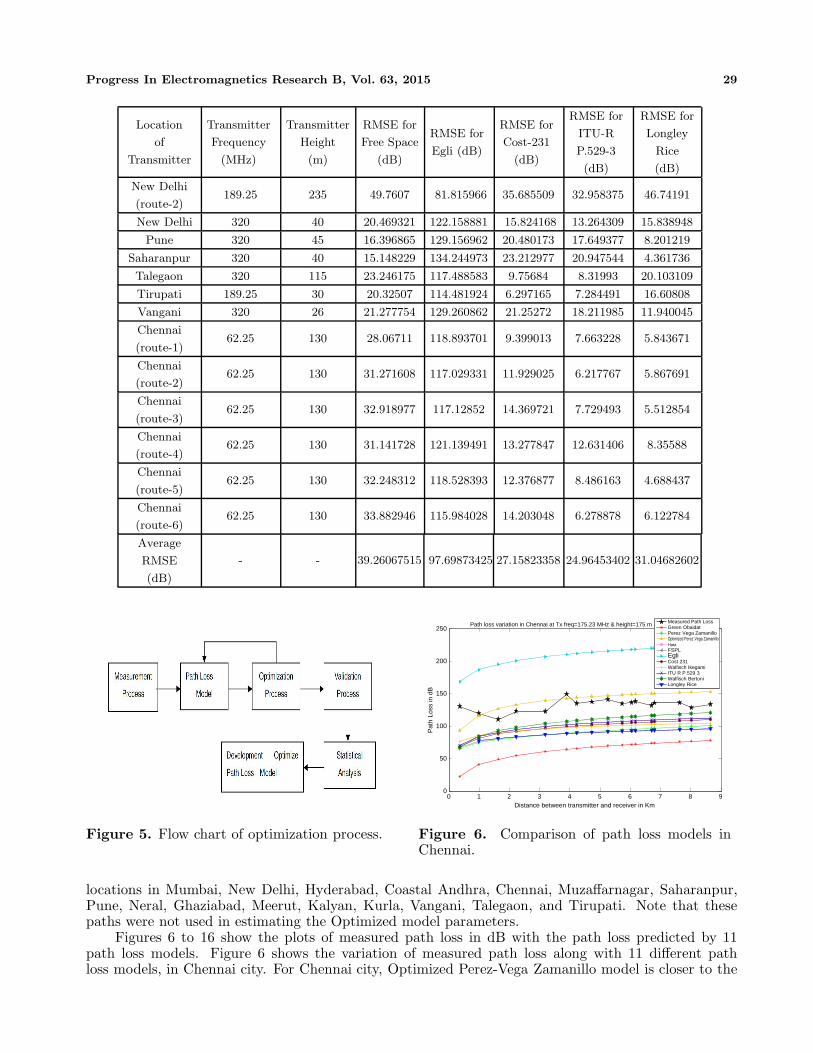
0 1 2 3 4 5 6 7 8 9Distance between transmitter and receiver in Km

Path loss variation in Chennai at Tx freq=175.23 MHz & height=175 m Measured Path LossGreen ObaidatPerez Vega ZamanilloOptimized Perez Vega ZamanilloHataFSPLEgliCost 231Walfisch IkegamiITU R P.529 3Walfisch BertoniLongley Rice

0

50

100

150

200

250

Pat

h Lo

ss in

dB

Figure 6. Comparison of path loss models inChennai.

locations in Mumbai, New Delhi, Hyderabad, Coastal Andhra, Chennai, Muzaffarnagar, Saharanpur,Pune, Neral, Ghaziabad, Meerut, Kalyan, Kurla, Vangani, Talegaon, and Tirupati. Note that thesepaths were not used in estimating the Optimized model parameters.

Figures 6 to 16 show the plots of measured path loss in dB with the path loss predicted by 11path loss models. Figure 6 shows the variation of measured path loss along with 11 different pathloss models, in Chennai city. For Chennai city, Optimized Perez-Vega Zamanillo model is closer to the

30 Bolli and Khan

5 10 15 20 25 30 35

Distance between transmitter and receiver in Km

Path loss variation in Talegaon at Tx freq=320 MHz & height=115 m

Measured Path LossGreen ObaidatPerez Vega ZamanilloOptimized Perez Vega ZamanilloHataFSPLEgliCost 231Walfisch IkegamiITU R P.529 3Walfisch BertoniLongley Rice

80

100

120

140

160

180

200

220

240

260

Pat

h Lo

ss in

dB

Figure 7. Comparison of path loss models inTalegaon.

0 5 10 15 20 25 30 35Distance between transmitter and receiver in Km

Path loss variation in Pune at Tx freq=320 MHz & height=45m


50

100

150

200

250

300

Pat

h Lo

ss in

dB

Figure 8. Comparison of path loss models inPune.

0 5 10 15 20 25 30 35 40 45 50Distance between transmitter and receiver in Km

Path loss variation in Saharanpur at Tx freq=320 MHz & height=40 mMeasured Path LossGreen ObaidatPerez Vega ZamanilloOptimized Perez Vega ZamanilloHataFSPLEgliCost 231Walfisch IkegamiITU R P.529 3Walfisch BertoniLongley Rice

50

100

150

200

250

300

Pat

h Lo

ss in

dB

Figure 9. Comparison of path loss models inSaharanpur

0 5 10 15 20 25Distance between transmitter and receiver in Km

Path loss variation in Vangani at Tx freq=320 MHz & height=26 m


50

100

150

200

250

300

Pat

h Lo

ss in

dB

Figure 10. Comparison of path loss models inVangani.

0 5 10 15 20 25 30Distance between transmitter and receiver in Km

Path loss variation in Hyderabad at Tx freq=224.25 MHz & height=150 m


-50

0

50

100

150

200

250

Pat

h Lo

ss in

dB

Figure 11. Comparison of path loss models inHyderabad.

0 5 10 15 20 25 30 35 40 45 50Distance between transmitter and receiver in Km

Path loss variation in Muzaffarnagar at Tx freq=320 MHz & height=40 mMeasured Path LossGreen ObaidatPerez Vega ZamanilloOptimized Perez Vega ZamanilloHataFSPLEgliCost 231Walfisch IkegamiITU R P.529 3Walfisch BertoniLongley Rice

50

100

150

200

250

300

Pat

h Lo

ss in

dB

Figure 12. Comparison of path loss models inMuzaffarnagar.

measured path loss values. Figure 11 shows the variation of path loss as a function of distance forDoordarshan (DD) TV tower located in Hyderabad along one radial. In this figure observed valuesare plotted from 0.5 km to 27 km. Optimized Perez-Vega Zamanillo model is found to give excellentagreement with observed values. All other models have large deviation with the observed path lossvalues. From Table 4 it is clear that Optimized Perez-Vega Zamanillo model has the best performancein Hyderabad city as it has the least RMSE of 7.44 dB, followed by Walfisch Bertoni model. Among the



Path loss variation in Coastal Andhra (Urban) at Tx freq=150 MHz & height=16 m


50

100

150

200

250

300

Pat

h Lo

ss in

dB

Figure 13. Comparison of path loss models inCoastal Andhra.


Path loss variation in New Delhi at Tx freq=189.25 MHz & height=235 mMeasured Path LossGreen ObaidatPerez Vega ZamanilloOptimized Perez Vega ZamanilloHataFSPLEgliCost 231Walfisch IkegamiITU R P.529 3Walfisch BertoniLongley Rice

0

50

100

150

200

250

300

Pat

h Lo

ss in

dB

Figure 14. Comparison of path loss models inNew Delhi.


Path loss variation in Meerut at Tx freq=320 MHz & height=40 mMeasured Path LossGreen ObaidatPerez Vega ZamanilloOptimized Perez Vega ZamanilloHataFSPLEgliCost 231Walfisch IkegamiITU R P.529 3Walfisch BertoniLongley Rice

50

100

150

200

250

300

Pat

h Lo

ss in

dB

Figure 15. Comparison of path loss models inMeerut.


Path loss variation in Mumbai at Tx freq=182.25 MHz & height=300 m


-50

0

50

100

150

200

250

Pat

h Lo

ss in

dB

Figure 16. Comparison of path loss models inMumbai.

11 path loss models discussed, Egli model has the worst performance in Hyderabad city as it has themaximum RMSE of 79.8 dB. Similarly, Figure 14 shows the variation of measured path loss and variouspath loss models w.r.t distance in New Delhi. For New Delhi city, Optimized Perez-Vega Zamanillomodel is in reasonable agreement with the measured path loss values. Figure 16 shows the variation ofmeasured path loss w.r.t distance and also of 11 different path loss models in Mumbai city. It is observedthat Optimized Perez-Vega Zamanillo model is closer to the measured path loss values. For Mumbaicity, Optimized Perez-Vega Zamanillo model has the least root mean square error. In [12], we foundthat Perez-Vega Zamanillo model is better model for India because it had the least RMSE of 16.93 dB.Therefore, Perez-Vega Zamanillo model was selected for Optimization in this paper. In our paper [12],we have considered 15 paths in India for comparison of different path loss models. In this paper, wehave the compared different path loss models with the measured path loss data, collected across 48different paths in India. We find that RMSE of Perez-Vega Zamanillo model increases from 16.93 dBin [12] to 28.9 dB. We can see that the performance of Optimized Perez-Vega Zamanillo model is bestin Hyderabad, Chennai, New Delhi, Ghaziabad, Mumbai, Meerut, and Vangani. Overall we can seethat performance of Optimized Perez-Vega Zamanillo model is best since it has the least average RMSEof 13.98 dB which is the least among the 11 path loss models discussed. Other path loss models overestimate the path loss because average root mean square error (RMSE) for other path loss models ismore than 24 dB. Therefore, Optimized Perez-Vega Zamanillo model is the best suited path loss modelfor India.

32 Bolli and Khan

6. CONCLUSION

In this paper, we have used the measurement data of path loss in (dB) at different distances fortransmitters in UHF/VHF bands, located at 21 different places in India. Optimized Perez-VegaZamanillo model is validated at different locations in Mumbai, New Delhi, Hyderabad, Coastal Andhra,Chennai, Muzaffarnagar, Saharanpur, Pune, Neral, Ghaziabad, Meerut, Kalyan, Kurla, Vangani,Talegaon, and Tirupati. We have compared the performance of 11 different known models with measureddata in terms of root mean square error (RMSE). RMSE obtained between Measured Path loss andthose predicted by the path loss models were compared across 48 routes in India. We can see thatthe performance of Optimized Perez-Vega Zamanillo model is best in Hyderabad, Chennai, New Delhi,Ghaziabad, Mumbai, Meerut, and Vangani. We found that performance of Optimized Perez-VegaZamanillo model is best as average root mean square error is 13.98 dB which is lowest when comparedto other models. Other path loss models over estimate the path loss because average root mean squareerror (RMSE) for other path loss models is more than 24 dB. India is a country with wide terrain andclimatic conditions. There is lot of variation in height of buildings in different cities of India. Also,there is a wide variation in sizes of cities in India. All these factors may have caused the RMSE of theoptimized model to become higher than the original model in some parts of India. We conclude thatOptimized Perez-vega zamanillo path loss model can be used in India for predicting coverage area forTVWS.

ACKNOWLEDGMENT

The research leading to this work was performed partly under the project “High PerformanceCognitive Radio Networks” funded by Department of Electronics and information Technology (DeitY),Government of India.

REFERENCES

1. First Report and Notice of Rulemaking in the Matter of Unlicensed Operation in TV BroadcastBands, ET Docket No. 04-186, Adopted Oct. 18, 2006.

2. Prasad, M. V. S. N. and I. Ahmad, “Comparison of some path loss prediction methods withVHF/UHF measurements,” IEEE Transactions on Broadcasting, Vol. 43, No. 4, 459–486, Dec. 1997.

3. Prasad, M. V. S. N. and R. Singh, “UHF train radio measurements in northern India,” IEEETransactions on Vehicular Technology, Vol. 49, No. 1, 239–245, USA, Jan. 2000.

4. Prasad, M. V. S. N. and R. Singh, “Terrestrial mobile communication train measurements inwestern India,” IEEE Transactions on Vehicular Technology, Vol. 52, No. 3, 671–682, May 2003.

5. Prasad, M. V. S. N., T. Rama Rao, I. Ahmad, and K. M. Paul, “Investigation of VHF signalsin bands I and II in southern India and model comparisons,” Indian Journal of Radio and SpacePhysics, Vol. 35, 198–205, Jun. 2006.

6. Prasad, M. V. S. N., “Path loss exponents deduced from VHF amp; UHF measurements over Indiansubcontinent and model comparison,” IEEE Transactions on Broadcasting, Vol. 52, No. 3, 290–298,2006.

7. Pathania, P., P. Kumar, and B. Shashi Rana, “Performance evaluation of different path loss modelsfor broadcasting applications,” American Journal of Engineering Research (AJER), Vol. 3, No. 4,335–342, 2014.

8. Pathania, P., P. Kumar, and B. Shashi Rana, “A modified formulation of path loss models forbroadcasting applications,” International Journal of Recent Technology and Engineering (IJRTE),Vol. 3, No. 3, 44–54, Jul. 2014.

9. Ying, X., C. W. Kim, and S. Roy, “Revisiting TV coverage estimation with measurement-basedstatistical interpolation,” http://www.dynamicspectrumalliance.org/assets/Revisiting TV Coverage Estimation with Measurement-based Statistical Interpolation 08202014.pdf.


10. Faruk, N., A. A. Ayeni, Y. Adediran, and N. Surajudeen-Bakinde, “Improved pathloss modelfor predicting TV coverage for secondary access,” International Journal of Wireless and MobileComputing, Vol. 7, No. 6, 565–576, 2014.

11. Mohammed Al Salameh, S. H., “Lateral ITU-R foliage and maximum attenuation models combinedwith relevant propagation models for forest at the VHF and UHF bands,”NNGT Int. J. onNetworking and Communication, Vol. 1, Jul. 2014.

12. Sridhar, B. and M. Z. A. Khan, “RMSE comparison of path loss models for UHF/VHF bands inIndia,” 2014 IEEE Region 10 Symposium, 330–335, Kuala Lumpur, Malaysia, Apr. 14–16, 2014.

13. Hata, M., “Empirical formula for propagation loss in land mobile radio services,” IEEE Trans.Vehicular Technology, Vol. 29, 317–325, 1980.

14. Farhoud, M., A. El-Keyi, and A. Sultan, “Empirical correction of the Okumura-Hata model forthe 900 MHz band in Egypt,” International Conference on Communications and InformationTechnology (ICCIT-2013): IEEE Wireless Communications and Signal Processing, 386–390,Beirut, Lebanon, Jun. 19–21, 2013.

15. Perez-Vega, C. and J. M. Zamanillo, “Path-loss model for broadcasting applications and outdoorcommunication systems in the VHF and UHF bands,” IEEE Transactions on Broadcasting, Vol. 48,No. 2, 91–96, Jun. 2002.

16. Roslee, M. B. and K. F. Kwan, “Optimization of Hata propagation prediction model in suburbanarea in Malaysia,” Progress In Electromagnetics Research C, Vol. 13, 91–106, 2010.

17. Egli, J. J., “Radio propagation above 40 MC over irregular terrain,” Proceedings of the IRE, Vol. 45,No. 10, 1383–1391, 1957.

18. Sharma, P. K. and R. K. Singh, “Comparative study of path loss model depends on variousparameter,” International Journal of Engineering Science and Technology, Vol. 3, 4683–4690,Jun. 2011.

19. Dayanand, A., K. Deepak, and P. Tejas, “Statistical tuning of Walfisch-Ikegami model in urban andsuburban environments,” Fourth Asia International Conference on AMS, 538–543, Kota Kinabalu,Malaysia, 2010.

20. ITU-R P.529-3, “VHF/UHF propagation data and prediction methods required for the terrestrialland mobile services,” 1994.

21. Green, D. B. and M. S. Obaidat, “An accurate line of sight propagation performance model for Ad-Hoc 802.11 wireless LAN (WLAN) devices,” Proceedings of IEEE ICC 2002, New York, Apr. 2002.

22. http://en.wikipedia.org/wiki/Free-space path loss.23. Rice, P. L., A. G. Longley, K. A. Norton, and A. P. Barsis, “Transmission loss predictions for

tropospheric communications circuits,” Technical Note 101, US Department of Commerce NTIA-ITS, 1967.

24. Rappaport, T. S., Wireless Communications Principles and Practice, Prentice Hall, 2002.25. Erceg, V., K. V. S. Hari, et al., “Channel models for fixed wireless applications,” Tech. Rep., IEEE

802.16 Broadband Wireless Access Working Group, Jan. 1986.

Documents

A Novel LMMSE Based Optimized Perez-Vega Zamanillo