Computers & Fluids 79 (2013) 105–119

Contents lists available at SciVerse ScienceDi rect

Computer s & Fluids

journal homepage: www.elsevier .com/ locate /compfluid

A novel Cartesian CFD cut cell approach

0045-7930/$ - see front matter � 2013 Elsevier Ltd. All rights reserved.http://dx.doi.org/10.1016/j.compfluid.2013.03.011

⇑ Tel.: +44 151 794 4818; fax: +44 151 794 4848.E-mail address: m.w.johnson@liv.ac.uk

Mark W. Johnson ⇑School of Engineering, University of Liverpool, Liverpool L69 3GH, UK

a r t i c l e i n f o a b s t r a c t

Article history:Received 22 October 2011 Received in revised from 14 February 2013 Accepted 22 March 2013 Available online 2 April 2013

Keywords:CFDCut cell Cartesian mesh

A new approach to evaluating the fluxes on the faces of Cartesian cut cells is presented. In contrast tomost established techniques where the value of a flow variable is only defined at specific points within a cell, in the new approach, the variable values are defined throughout the cell using spline functions. This ensures the first derivatives of the flow variables are continuous throughout the computational domain which is not achieved with existing finite volume methods. For cut cells the values of the variables along the cut faces are therefore defined and hence the mass and momentum fluxes are readily evaluated tosecond order accuracy. The method is validated against three test cases where analytical solutions orextensive experimen tal and comp utational data exists. The test cases are flow in an annulus, flow around an isolated cylinder and laminar boundary layer developm ent on a flat plate inclined at a range of angles to the gridlines. For these test cases, the flow is accurat ely resolved in the cut cells. The method therefore realises the potential of Cartesian CFD as a more efficient computational tool than more commonly used body fitted methods.

� 2013 Elsevier Ltd. All rights reserved.

1. Introduction

The majority of CFD calculations are currently performed onbody fitted meshes, which provide good resolution of the boundary layers providing an adequate ly fine grid is used and suitable cell types are used in the near wall region. The definition of a suitable grid for a complex engineering geometry can be a laborious task however and frequent ly requires a high degree of expertise and experience. As the capabilities of CFD have increased and hence the complexi ty of the engineeri ng geometries which can be com- puted, simpler alternativ es to body fitted meshes have been sought. Two alternatives have shown promise. The first approach is to abandon the mesh altogether and to use a meshless approach ,e.g. Shu et al. [1,2]. These methods use a finite differenc e rather than a finite volume formulation however, which means they have the disadvantages of being non-conservat ive. These methods have potential, but a full discussion is beyond the scope of the present paper. The second approach is the Cartesian grid approach where the flow domain is divided into simple squares in 2-d or cubes in3-d.

Cartesian CFD methods have several advantag es over methods that use a body fitted mesh. Firstly, the meshing process is consid- erably more straightforwar d and easily automated and hence the time taken to mesh a complex engineering geometry is signifi-cantly reduced. Secondly, the finite volume flow equation s are sim- pler as the mass flux through each face depends on only one

velocity component rather than all components and finally, the additional computational effort involved in problems with moving boundari es is greatly reduced because, after each time step, only the cells adjacent to the moving boundary need to be adapted rather than the whole mesh. Cartesian methods do however have one major drawback, which is that when conventi onal finite vol- ume procedures are used, accuracy is compromi sed in the cut cells on the boundaries particular ly for Navier Stokes solutions. This isoften of critical importance in CFD because the boundary layers are responsible for the aerodyna mic losses and hence any error in these regions leads to inaccurate predictio n of performance. This problem is not restricted to Cartesian grids and is also apparent inbody fitted schemes when cells, other than body fitted quadrilater- als (e.g. triangles), are used adjacent to wall boundari es.

A variety of approach es have been adopted to improve the res- olution of boundary layers in cut cells which can be divided into two categories [3]. The first category of methods, which was insti- gated by Peskin [4], retains full cells straddling the boundaries and introduce s a forcing function which modifies the flow adjacent tothe boundary in order to satisfy the required boundary condition .These methods have been developed by Peskin and other research- ers [5–14] but as the technique is not conservative the disadvan- tages associated with non-conservat ive schemes are inherited.The second category of methods uses the unmodified flow equa- tions and so the solutions are conservative, but the fluxes through the cut faces need to be determined. These Cartesian methods have had considerable success for Euler flow solutions, e.g. Nemec et al.[15]. In Euler flows the necessity to resolve the high velocity shear rate, which results within the boundary layers, is avoided and

Fig. 2. Error in continuity equation for cells cut at different heights and angles.Black lines – 2nd order scheme and grey lines – spline scheme.

106 M.W. Johnson / Computers & Fluids 79 (2013) 105–119

hence the modest gradients in flow properties across the cut cells adjacent to the boundary lead to acceptably small truncation er- rors. Boundary layer effects have been added to these calculations ,e.g. Aftosmis et al. [16] by undertak ing boundary layer calculations on 2-d planes aligned with the flow. This approach is applicable tocomputation of flow around streamline bodies providing the boundary layers remain attached or only mildly separated and the boundary layer flow is not significantly skewed by 3-d effects.The method is however not more generally applicable to flowswhere a full Navier Stokes solution is needed. Full Navier Stokes solutions have been obtained using embedded body fitted grids within the boundary layers, e.g. Cai et al. [17]. This displaces the cut cell resolution problem beyond the edge of the boundary layer where the flow variable gradients are once again weaker and hence any inaccuracies where the Cartesian and embedde d meshes over- lap are greatly reduced. This approach is however difficult to apply to general flow geometries where no a priori knowledge of the ex- tent of the boundary layer regions exists, particularly where boundary layer separation is present. The implementation of the embedded grid is also complex in comparison with a pure Carte- sian scheme and so much of the simplicity of the pure Cartesian meshing is lost. Hartmann et al. [18] use a pure Cartesian mesh and developed a conservati ve method for cut cells which they have applied successfully to 3-d compressib le viscid flow. A least squares approach , similar to that used in meshless methods, isadopted for evaluation of the fluxes through the cut faces.

There are strong motives to develop improved finite volume schemes for Cartesian grids which retain high accuracy within the cut cells on the boundaries. The objective of the current work was to develop a second order accurate procedure for determining the fluxes through the cut faces which could be implemented eas- ily and systematical ly in both two and three dimensions.

1.1. Solution accuracy in cut cells

In developing new methods for cut cells, it is useful to consider why many current approaches lead to poor accuracy. A sloping boundary and the resulting cut cells for a Cartesian grid are shown in Fig. 1. For a simple second order accurate finite volume scheme,the values of velocity at the points w, e and n on the faces are cal- culated as the average of the values in the two adjacent cells C andW, C and E and C and N. This will only give the correct flux through the face if the velocity varies linearly along the face length and the points w, e and n lie in the centres of their respective faces. When the boundary is parallel with the gridlines, i.e. a = 0, any error asso- ciated with the flux will be approximately the same on the w and e

Fig. 1. Cut cell geometry.

faces and so this will cancel out when the continuity and momen- tum balances are considered. However, when a–0 this is not the case as the deviation of the w and e points from the midpoint will differ. It should be noted that this is not a source of error for the nface in the current example as this face is uncut. To determine the magnitud e of the error and its depende nce on the cut angle a, con- sider the algebraic solution to the continuity and momentum equation s at infinite Reynolds number

U ¼ 2X�12Y V ¼ X�

32Y2 p ¼ 0 ð1Þ

where U and V are the wall parallel and normal veloc ities in the Xand Y direction as indicated in Fig. 1. Close to the wall this solution has the characterist ics of a boundary layer. The velocity compo- nents at the cell centres can then be determine d as

uði; jÞ ¼ ðDxÞ12ði cos aþ j sinaÞ

�32 ð�i sin aþ j cos aÞ½ið1

þ cos2 aÞ þ j sina cos a� ð2Þ

vði; jÞ ¼ ðDxÞ12ði cos aþ j sin aÞ

�32 ð�i sinaþ j cos aÞ½i sin a cos a

þ jð1þ sin2 aÞ� ð3Þ

where i and j are the cell indices. These values can then be used todetermine a resultan t error in the continuity equation using the 2nd order approxim ation to the face values (i.e. the average of adjacent cell values). This error is assumed to be similar in magnitud e to the error that would result in satisfying the continuity equation if the finite volume equation s were solved. The results are shown inFig. 2 for X = 1000 Dx and 10� increments of the cut face angle awith different heights of cut through the cell (cell volume). The re- sults clearly show that the error for any non zero angle a is about two orders of magnitude higher than the a = 0 case. It is also appar- ent that to overcome this problem the strong variation in the flowquanti ties along the cell faces must be taken into account.

2. The new method

2.1. Cartesian mesh generatio n

The Cartesian meshes for the current study were generate dusing established procedures. A structured Cartesian mesh in two dimensio ns can be produced simply by dividing the whole flow do- main into a number of identical square cells. Boundary nodes are then defined at each point where a mesh line crosses the flow do- main and for simplicity these nodes are connected with straight edges. This leads to rounding of any sharp corners in the domain boundary , but for realistic grids this will not compromise the

Fig. 3. Cell merging algorithm.

Fig. 4. Full cell surrounded by eight cell values.

M.W. Johnson / Computers & Fluids 79 (2013) 105–119 107

definition of the domain boundary significantly. Cells that intersect with the flow domain boundaries (the cut cells) will have a smaller volume than the uncut cells (full cells) which cover the majority ofthe domain. Cut cells which have much smaller volumes are anundesirable feature as the CFL condition would require a signifi-cantly smaller time step during the CFD solution. For this reason,in the current method, cut cells whose cell centre lie outside the flow domain, i.e. which have a volume less than half the full cell volume, are merged with the adjacent cell which shares the longest boundary with the cut cell. When these cells share a boundary node this is deleted, which leads to further rounding of sharp cor- ners in the flow domain boundary and may also lead to a cell cen- tre for the merged cell outside the flow domain. If this is the case the cell undergoes a further merging along its longest shared boundary. Every merged cell therefore ultimately consists of a par- ent whose cell centre lies within the flow domain and one or two children whose cell centres lie outside the flow domain. An exam- ple of this process is shown in Fig. 3. Four cells C, N, NE and E areshown where the boundary defined by the original geometry cuts the N, NE and E cells such that each of their cell centres lies outside the flow domain. The point defining the corner in the original geometry within the NE cell is not retained which, prior to cell merging, leads to the initial boundary shown in the figure. The firstpass of the merging algorithm will lead to the combination of cells C and N and cells E and NE. The cell centres of both E and NE areoutside the flow domain and hence the combined E/NE cell under- goes a further merging with C/N during a second pass of the algo- rithm. The combined merging will also lead to the deletion of the two node points between NE and its neighbours resulting in the fi-nal boundary in Fig. 3. The four original cells have thus been re- duced to a single cell where C is the parent and the remnants ofN and E are the children.

It should be noted that, although not implemented here, any structured Cartesian grid can be refined to produce an unstruc- tured grid using a quadtree structure whereby cells are succes- sively subdivided into quarters. Both the merging and subdivision methodol ogies are easily extended to three dimensions .

2.2. Finite volume equations

In the current work the 2-d unsteady incompress ible RANS equations are solved using a conservati ve finite volume formula- tion. The presentation of the methodol ogy is therefore limited to2-d incompressible flow, however extension to 3-d is discussed un- der future work and the methodology can also be used for com- pressible flow. The majority of existing approaches to forming finite volume equation s consider the value of each flow variable q at discrete points in space. q is defined at the storage locations (typically the cell centres or corners) and values required for the fluxes are then determined on the cell faces using Taylor series

approximat ions. The value of q elsewhere in the cell and in partic- ular the variation in q over the cell face is not generally considered and so q is often discontinuo us in value and almost always discon- tinuous in its first derivatives between adjoining cell faces. When the cells are approximately rectangular in shape, the cell face value is effectively evaluated at a point close to the centre of the cell face and is therefore a good approximat ion (usually second order) tothe cell face average value and therefore the cell fluxes are accu- rately determined . However, as demonstrat ed above, if the cells deviate significantly from a rectangu lar shape, there is a conse- quential degradat ion in accuracy. This problem can be addresse dby using a scheme whereby the flow variables are defined at all points within the flow domain and (at a minimum) their firstderivatives are also continuous within the flow domain. This isachieved in the current work by defining the variation of each flowvariable q throughout each cell using spline functions. As the value of q is also defined in this way within the cut cells then the varia- tion in q over the cut faces required to determine the flux is known.

2.2.1. Full cells To begin with consider a full cell which is surrounded by a com-

plete set of eight full cells as shown in Fig. 4. The value of the var- iable q is stored in each cell, but it should be noted that this is not the value of q given by the spline function at the cell centre. This value will be determined later. The value and first derivatives can now be determined to second order at each mesh point interms of the values stored in the four surrounding cells using Tay- lor series. For example for mesh point nw in Fig. 4.

qnw ¼ðqW þ qC þ qNW þ qNÞ

4ð4Þ

@q@x

� �nw

¼ ðqN þ qC � qNW � qWÞ2Dx

ð5Þ

@q@y

� �nw¼ ðqN þ qNW � qC � qWÞ

2Dyð6Þ

and also

@2q@x@y

!nw

¼ ðqN þ qW � qNW � qCÞDxDy

ð7Þ

The value for each variable q at any point in the cell can now bedefined using the cubic spline equation

Fig. 5. Determining values at the nw mesh point near a boundary where (a) one surrounding cell value is absent and (b) two surrounding cell values are absent.

108 M.W. Johnson / Computers & Fluids 79 (2013) 105–119

qðx; yÞ ¼ f0ðxÞf0ðyÞqsw þ f1ðxÞf0ðyÞqse þ f0ðxÞf1ðyÞqnw

þ f1ðxÞf1ðyÞqne þ g0ðxÞf0ðyÞ@q@x

� �sw

þ g1ðxÞf0ðyÞ@q@x

� �seþ g0ðxÞf1ðyÞ

@q@x

� �nw

þ g1ðxÞf1ðyÞ@q@x

� �neþ f0ðxÞg0ðyÞ

@q@y

� �sw

þ f1ðxÞg0ðyÞ@q@y

� �seþ f0ðxÞg1ðyÞ

@q@y

� �nw

þ f1ðxÞg1ðyÞ@q@y

� �ne

þ g0ðxÞg0ðyÞ@2q@x@y

!sw

þ g1ðxÞg0ðyÞ@2q@x@y

!se

þ g0ðxÞg1ðyÞ@2q@x@y

!nw

þ g1ðxÞg1ðyÞ@2q@x@y

!ne

ð8Þ

where the functions f0, f1, g0 and g1 are given by

f0ðxÞ ¼ðx� 1Þ2ð2xþ 1Þ

ðDxÞ3; f 1ðxÞ ¼

x2ð3� 2xÞðDxÞ3

;

g0ðxÞ ¼xðx� 1Þ2

ðDxÞ2and g1ðxÞ ¼

x2ðx� 1ÞðDxÞ2

ð9Þ

and the origin for x and y is the sw mesh point.The value of q determined from the spline functions at the cell

centre is therefore

14ðqsw þ qse þ qnw þ qneÞ

þ Dx16

@q@x

� �sw� @q

@x

� �seþ @q

@x

� �nw� @q

@x

� �ne

� �

þ Dy16

@q@y

� �swþ @q

@y

� �se� @q

@y

� �nw� @q

@y

� �ne

� �

þ DxDy64

@2q@x@y

!sw

� @2q@x@y

!se

� @2q@x@y

!nw

þ @2q@x@y

!ne

!

¼ 916

qC þ3

32ðqW þ qE þ qN þ qSÞ þ

164ðqSW þ qSE þ qNW þ qNEÞ

ð10Þ

The cubic spline formulation ensures that the value and firstderivatives are continuous across cell boundari es. The volume fluxthrough the vertical face between the mesh points sw and nw istherefore given byZ y¼Dy

y¼0udy ¼

Z y¼Dy

y¼0f0ðyÞusw þ f1ðyÞunw þ g0ðyÞ

@u@y

� �sw

�

þg1ðyÞ@u@y

� �nw

�dy

¼ 12ðusw þ unwÞ þ

Dy12

@u@y

� �sw

� @u@y

� �nw

� �� �Dy

¼ 13ðuW þ uCÞ þ

112ðuSW þ uS þ uNW þ uNÞ

� �Dy ð11Þ

and so is dependent on the six cell values nearest to that face.This formulation therefore differs from a conventi onal second

order finite volume approximat ion as the variation of u in both the x and y direction is considered. It seems entirely appropriate however to improve accuracy by including additional cell values in their order of proximity to the face being considered . The full fi-nite volume equations for mass and momentum will therefore use a nine point template consisting of the current cell value and the values from the surroundi ng eight cells. The template involves

more points than the seven points required for a conventional sec- ond order upwind scheme however the coefficients are simpler toevaluate than for a body fitted grid and for full cells in 2-d there are only three coefficient values, for the centre point C, offset points (W, E, N and S) and diagonal points (NW, NE, SW and SE). This in- creases to five coefficient values in 3-d. There is therefore an in- creased computational overhead when compared with aconventi onal Cartesian grid formulat ion, however the computa- tional cost is still considerabl y less than for a body fitted grid sys- tem. For consistency and simplicit y in coding, this nine point template is maintained for cells close to the boundaries where some of the surrounding eight cell values are no longer available.

2.2.2. Boundaries For mesh points close to the boundaries, Eqs. (4)–(7) cannot be

used because either one or two of the surrounding cells are cut such that they no longer store a value. These situations are shown in Fig. 5 where for the mesh point nw the value in the cell NW(Fig. 5a) or the values in the cells NW and N (Fig. 5b) are not stored.If a boundary condition for q is available on the cut face for all the cut cells surroundi ng the mesh point then these boundary condi- tion values at the points where the diagonal intersects the bound- ary can be used in place of each missing cell stored value as shown in Fig. 6. The revised equation s which replace Eqs. (4)–(7) can then be derived from the Taylor series to obtain

qnw¼1

ðfNfCþ fNW fCÞðfNW fW fCqNþ fNfW fCqNW þ fNfNW fCqW þ fNfNW fW qCÞ

ð12Þ

@q@x

� �nw

¼ 12DxðfNfCþ fNW fCÞ

f 2W þ fNW fCþ fWðfC� fNWÞ

ðfNþ fW ÞqN

�

� f 2C þ fNfW þ fCðfW � fNÞ

ðfNW þ fCÞqNW �

f 2N þ fNW fCþ fNðfNW � fCÞ

ðfNþ fWÞqW

þ f 2NW þ fNfW þ fNWðfC� fWÞ

ðfNW þ fCÞqC

�ð13Þ

@q@y

� �nw

¼ 12DyðfNfCþ fNW fCÞ

f 2W þ fNW fCþ fWðfNW � fCÞ

ðfNþ fWÞqN

�

� f 2C þ fNfW þ fCðfN� fWÞ

ðfNW þ fCÞqNW �

f 2N þ fNW fCþ fNðfC� fNWÞ

ðfNþ fWÞqW

þ f 2NW þ fNfW þ fNWðfW � fCÞ

ðfNW þ fCÞqC

�ð14Þ

and

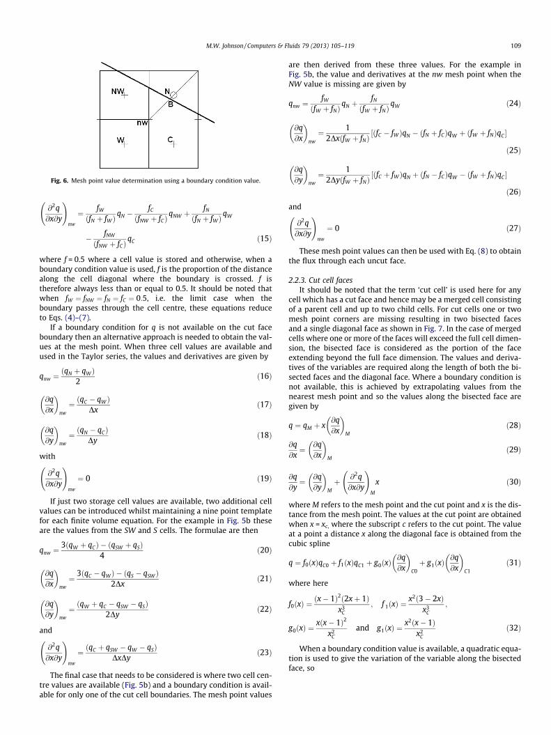
Fig. 6. Mesh point value determination using a boundary condition value.

M.W. Johnson / Computers & Fluids 79 (2013) 105–119 109

@2q@x@y

!nw

¼ fW

ðfN þ fWÞqN �

fC

ðfNW þ fCÞqNW þ

fN

ðfN þ fWÞqW

� fNW

ðfNW þ fCÞqC ð15Þ

where f = 0.5 where a cell value is stored and otherwis e, when aboundary condition value is used, f is the proportio n of the distance along the cell diagonal where the boundar y is crossed. f istherefore always less than or equal to 0.5. It should be noted that when fW ¼ fNW ¼ fN ¼ fC ¼ 0:5, i.e. the limit case when the boundary passes through the cell centre, these equations reduce to Eqs. (4)–(7).

If a boundary condition for q is not available on the cut face boundary then an alternative approach is needed to obtain the val- ues at the mesh point. When three cell values are available and used in the Taylor series, the values and derivatives are given by

qnw ¼ðqN þ qWÞ

2ð16Þ

@q@x

� �nw

¼ ðqC � qW ÞDx

ð17Þ

@q@y

� �nw¼ ðqN � qCÞ

Dyð18Þ

with

@2q@x@y

!nw

¼ 0 ð19Þ

If just two storage cell values are available, two additional cell values can be introduced whilst maintaining a nine point template for each finite volume equation. For the example in Fig. 5b these are the values from the SW and S cells. The formulae are then

qnw ¼3ðqW þ qCÞ � ðqSW þ qSÞ

4ð20Þ

@q@x

� �nw¼ 3ðqC � qWÞ � ðqS � qSWÞ

2Dxð21Þ

@q@y

� �nw

¼ ðqW þ qC � qSW � qSÞ2Dy

ð22Þ

and

@2q@x@y

!nw

¼ ðqC þ qSW � qW � qSÞDxDy

ð23Þ

The final case that needs to be considered is where two cell cen- tre values are available (Fig. 5b) and a boundary condition is avail- able for only one of the cut cell boundaries. The mesh point values

are then derived from these three values. For the example inFig. 5b, the value and derivatives at the nw mesh point when the NW value is missing are given by

qnw ¼fW

ðfW þ fNÞqN þ

fN

ðfW þ fNÞqW ð24Þ

@q@x

� �nw

¼ 12DxðfW þ fNÞ

½ðfC � fWÞqN � ðfN þ fCÞqW þ ðfW þ fNÞqC �

ð25Þ

@q@y

� �nw

¼ 12DyðfW þ fNÞ

½ðfC þ fWÞqN þ ðfN � fCÞqW � ðfW þ fNÞqC �

ð26Þ

and

@2q@x@y

!nw

¼ 0 ð27Þ

These mesh point values can then be used with Eq. (8) to obtain the flux through each uncut face.

2.2.3. Cut cell faces It should be noted that the term ‘cut cell’ is used here for any

cell which has a cut face and hence may be a merged cell consisting of a parent cell and up to two child cells. For cut cells one or two mesh point corners are missing resulting in two bisected faces and a single diagonal face as shown in Fig. 7. In the case of merged cells where one or more of the faces will exceed the full cell dimen- sion, the bisected face is considered as the portion of the face extendin g beyond the full face dimension. The values and deriva- tives of the variables are required along the length of both the bi- sected faces and the diagonal face. Where a boundary condition isnot available, this is achieved by extrapolati ng values from the nearest mesh point and so the values along the bisected face are given by

q ¼ qM þ x@q@x

� �M

ð28Þ

@q@x¼ @q

@x

� �M

ð29Þ

@q@y¼ @q

@y

� �M

þ @2q@x@y

!M

x ð30Þ

where M refers to the mesh point and the cut point and x is the dis- tance from the mesh point. The values at the cut point are obtained when x = xc, where the subscript c refers to the cut point. The value at a point a distance x along the diagonal face is obtained from the cubic spline

q ¼ f0ðxÞqC0 þ f1ðxÞqC1 þ g0ðxÞ@q@x

� �C0þ g1ðxÞ

@q@x

� �C1

ð31Þ

where here

f0ðxÞ ¼ðx� 1Þ2ð2xþ 1Þ

x3C

; f 1ðxÞ ¼x2ð3� 2xÞ

x3C

;

g0ðxÞ ¼xðx� 1Þ2

x2C

and g1ðxÞ ¼x2ðx� 1Þ

x2C

ð32Þ

When a boundary condition value is available , a quadratic equa- tion is used to give the variation of the variable along the bisected face, so

Fig. 7. Examples of cut cell types.

110 M.W. Johnson / Computers & Fluids 79 (2013) 105–119

qðxÞ ¼ 1� xxC

� �2 !

qM þxxC

� �2

qC þ x 1� xxC

� �@q@x

� �M

ð33Þ

and the boundary conditio n value is used on the diagonal face.

2.2.4. Cut cell errors The error in the continuity equation for the range of cut cells,

already considered using a simple 2nd order finite volume scheme,was determined using the new method. The results are also shown in Fig. 2 and indicate that, for all cut angles, the resultant error re- mains below that achieved at a = 0 for the conventional 2nd order scheme. The objective of devising an accurate finite volume formu- lation for cut cells therefore appears to have been achieved. It has been assumed though that solution of the flow equation s using the new method will result in errors similar to the ones calculated inFig. 2 from an exact flow solution. Full CFD solutions are required to validate the new method.

2.3. Solution procedure

In the current work, the unsteady 2-d RANS equation s are solved, but the methodology is readily applied to any form ofconservation equations. A conventional two step pressure correc- tion method following Voke and Yang [19] is used to solve the equations. In the first step, the velocity is marched explicitly intime using the velocity terms in the momentum equations. The time derivative is evaluated to second order accuracy in time by utilising the momentum flux from the previous time level.Thus

utþDt ¼ ut þ32

@u@t

� �t

� 12

@u@t

� �t�Dt

� �Dt ð34Þ

In the second step, the pressure is corrected such that the resul- tant change in the velocity from the momentum equation satisfiesthe continuity equation. The resulting Poisson equation in pressure is solved using point over-relaxation.

The finite volume templates using the new method involve more points than a conventional 2nd order method and are therefore more laborious to compute. The template s for the lin- ear terms in the equation s, which remained invariant throughout the calculation, were evaluated at the start and stored in mem- ory. These are the templates for u and v in the continuity equa- tion and for p in the x and y momentum equations. It should benoted that the templates for all full cells, which are surrounded by eight storage cells, i.e. the majority of internal cells, are iden- tical and hence the storage requiremen t is largely for the cut cells which, for typical geometri es, are less than 10% of the total cell count.

A flow solution is judged to be sufficiently accurate once the residuals to the continuity and momentum equations have been

reduced by at least three orders of magnitude from their initial values. Typically this requires sufficient time steps for the flow totravel through the geometry at least five times.

3. Test cases

Current Cartesian grid formulation s lead to poor resolution of the flow in the cut cells and so test cases were chosen spe- cifically to determine whether the current formulat ion over- comes this deficiency.

3.1. Test case 1

The first test case was chosen to test the accuracy of the current method for highly curved boundaries. The geometry is shown inFig. 8 and consists of an annular channel of inner and outer radii ri and ro respectively. Both the inner and outer boundari es are sta- tionary walls and flow is induced by introducing a discontinuity inpressure along the right hand horizontal radius. For laminar flowthis flow has the analytical solution

uh

�u¼ r2

o lnrro

� �� r2

i lnrri

� �� �r þ r2

i r2o ln

ro

ri

� �1r

� ��

�14

r2o � r2

i

� �2 þ r2i r2

o lnro

ri

� �� �2" #

ð35Þ

where �u is the bulk tangentia l velocity. The flow solution is inde- penden t of the Reynolds number. Calculations were performed for outer to inner radius ratios of 3 and 6 using the coarse and fine grids shown in Fig. 8, which have cell sizes of 0.1 ro and 0.05 ro respec-tively. Velocity vector plots of the results are shown in Fig. 9 andthe tangential velocities determine d for all mesh points are plotted in Fig. 10. The latter figure shows a slight dependenc e on angula rposition just for the coarse grid and radius ratio of 6 close to the in- ner radius. This is due to the poor grid definition of the inner radius for this case which is apparen t in Fig. 8. There is also a small differ- ence between the calculate d values and the analytical solution for the coarse grid and the radius ratio of 3, but there is no indication of any dependenc e on angular position. The results on the fine grid for both radius ratios are within 1% of the analytic al solution.

In order to check that the calculations were of second order accuracy, a mesh convergence test was performed for the radius ratio of 6 for mesh sizes from 0.01 ro to 0.1 ro. The error, computed as the average absolute value of the difference between the analyt- ical and numerica l solutions, for both the tangential and radial velocity components is shown in Fig. 11. The error values correctly follow the trend line for a second order scheme. A further test was performed using the wall shear stress in order to confirm that sec- ond order accuracy is achieved in the cut cells alone. The average absolute error in the wall shear stress is plotted in Fig. 11. The wall

Fig. 9. Velocity vectors on coarse and fine grids for radius ratios of 3 and 6.

Fig. 8. Coarse and fine grids for outer to inner radius ratios of 3 and 6.

M.W. Johnson / Computers & Fluids 79 (2013) 105–119 111

Fig. 12. Grid for cylinder test case.

Fig. 11. Grid convergence test for annular flow.

Fig. 10. Theoretical and numerical velocity distribution for coarse and fine grids and radius ratios of 3 and 6.

112 M.W. Johnson / Computers & Fluids 79 (2013) 105–119

shear stress depends on the velocity gradient and hence for second order accuracy in velocity, the wall shear stress error should follow the first order trend line. This is the case for all but the coarsest grid, where the poor definition of the inner wall shown in Fig. 8leads to an error on the inner wall which is more than four times greater than that on the outer wall. In comparison, for the finermeshes the error on the inner wall is only about 50% greater. These results therefore demonst rate that the cut cell methodol ogy presented in this paper achieves second order solution accuracy for highly curved boundaries.

3.2. Test case 2

The flow around an isolated cylinder of diameter D is chosen asthe second test case as there is a large quantity of experimental and numerical data available for validation. The uniform computa- tional grid shown in Fig. 12 uses a mesh size of 0.1 D and extends to10 D upstream, above and below the cylinder and to 20 Ddownstre am. A uniform flow boundary condition was imposed up- stream with constant pressure boundary condition s on the other three outer boundari es. Calculations were performed at Reynolds numbers of 20, 40, 50, 80 and 300. Velocity vector plots for the region close to the cylinder and for the near wake are shown inFig. 13. Experimental observations Wieselsber ger [20] and

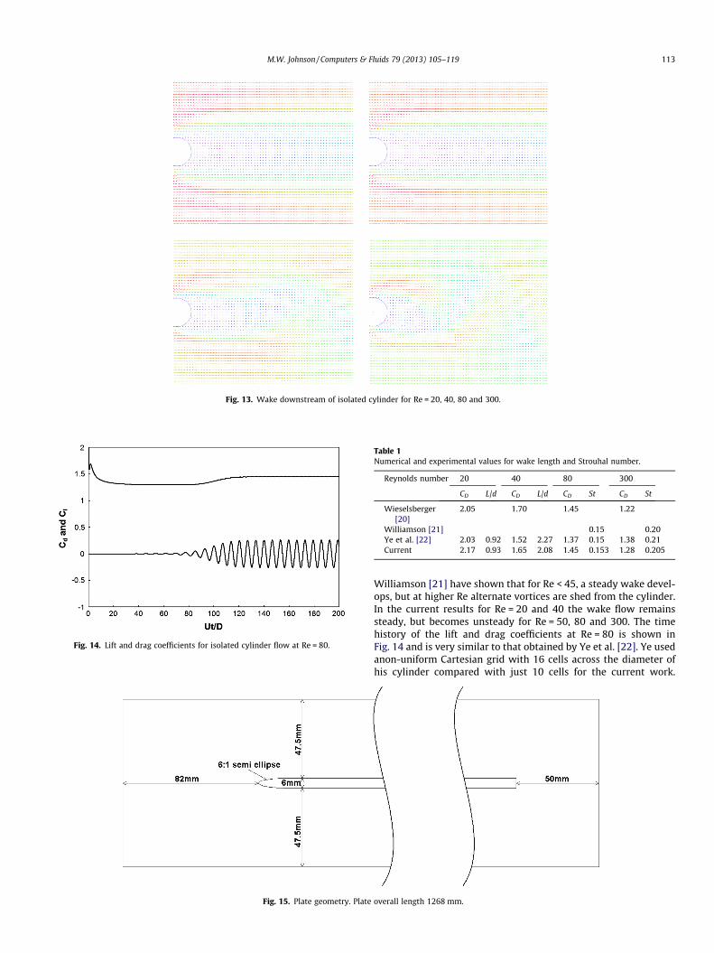
Fig. 13. Wake downstream of isolated cylinder for Re = 20, 40, 80 and 300.

Fig. 14. Lift and drag coefficients for isolated cylinder flow at Re = 80.

Table 1Numerical and experim ental values for wake length and Strouhal number.

Reynolds number 20 40 80 300

CD L/d CD L/d CD St CD St

Wieselsberger[20]

2.05 1.70 1.45 1.22

Williamson [21] 0.15 0.20 Ye et al. [22] 2.03 0.92 1.52 2.27 1.37 0.15 1.38 0.21 Current 2.17 0.93 1.65 2.08 1.45 0.153 1.28 0.205

Fig. 15. Plate geometry. Plate

M.W. Johnson / Computers & Fluids 79 (2013) 105–119 113

Williamson [21] have shown that for Re < 45, a steady wake devel- ops, but at higher Re alternate vortices are shed from the cylinder.In the current results for Re = 20 and 40 the wake flow remains steady, but becomes unsteady for Re = 50, 80 and 300. The time history of the lift and drag coefficients at Re = 80 is shown inFig. 14 and is very similar to that obtained by Ye et al. [22]. Ye used anon-uniform Cartesian grid with 16 cells across the diameter ofhis cylinder compared with just 10 cells for the current work.

overall length 1268 mm.

Fig. 16. Leading edge detail for 0�, 10�, 20�, 30� and 40� grids.

114 M.W. Johnson / Computers & Fluids 79 (2013) 105–119

The unsteadines s is much weaker at Re = 50 with peak to peak variations in CL of 10�4 at a Strouhal number of 0.083. Table 1shows the wake extent L, measure d to the detached stagnation point, for the steady wakes and the Strouhal numbers St for higher Re values for the current work, the experimental results Wiesels- berger [20] and Williamson [21] and the numerical work of Yeet al. [22]. The current values are very similar to these published results hence confirming that the numerical approach provides accurate results for this test case.

Fig. 17. Determination of freestream velocity.

3.3. Test case 3

The third test case is the developmen t of a laminar boundary layer on the flat plate shown in Fig. 15. The plate is 1268 mm inlength with a thickness of 6 mm and has a semi elliptic 6:1 leading edge. Five grids were used each consisting of approximat ely 140,000 1 mm � 1 mm cells where the gridlines were at angles of 0�, 10�, 20�, 30� or 40� to the plate surface. These five angles cov- er the full range of possible grids formed when the gridlines are ro- tated in increments of 10� through a full 360 �. Detail of the leading edge region for each of the grids is shown in Fig. 16. A wide range of cut cell and parent/child merged cells are present. A uniform flow inlet condition was applied on the boundary upstream ofthe plate with constant pressure outlet conditions applied on the boundaries above, below and downstream of the plate. The flowgeometry and boundary conditions were identical for the five grids such that the effect on the flow solution of rotating the gridlines

could be assessed. The flow was computed on each of the five grids for plate Reynolds numbers of 25,000, 62,500 and 125,000 (threedifferent viscosities). Boundary layer profiles were extracted atten streamw ise stations along the plate for each flow. For each pro- file the velocity values were determined using the spline functions at points where the measureme nt plane intersected each gridline.The boundary layer integral parameters were then obtained through numerical integration of the profiles. The integral param- eters are highly sensitive to the value of freestream velocity used intheir calculation and so an accurate algorithm is required. The velocity was averaged starting from the outermost freestrea m

Fig. 18. Boundary layer development for Reynolds numbers of 25,000, 62,500 and 125,000. Black symbols – upper and grey symbols – lower boundary layer.

Fig. 19. Boundary layer shape factors for Reynolds numbers of 25,000, 62,500 and 125,000. Black symbols – upper and grey symbols – lower boundary layer.

M.W. Johnson / Computers & Fluids 79 (2013) 105–119 115

velocity and this average value was compared with the local value and the local velocity gradient once the maximum velocity in the profile had been passed as shown in Fig. 17. The edge of the bound- ary layer was defined as the point where the local velocity was less than the integrated average velocity and the velocity gradient was greater than 5% of the gradient obtained by dividing the local velocity by the distance from the wall. The integrated average

velocity at this point is then used as the freestrea m velocity in eval- uating the boundary layer integral parameters. This definition en- sures only the flow inside the boundary layer contributes to the displacemen t thickness.

The predicted developmen t of the boundary layer along the plate for all 15 cases is shown in Fig. 18 together with the theoret- ical Blasius prediction. It can be seen that there is virtually no

116 M.W. Johnson / Computers & Fluids 79 (2013) 105–119

difference between the results for the different grids at the lowest Reynolds number, but as the Reynolds number is increased some grid dependence is apparent. The discrepancy appears to be largely due to incorrect prediction of the boundary layer developmen tclose to the leading edge as if the points on each grid were plotted using a different origin for Rex then they would lie much closer tothe theoretical Blasius curve for the higher plate Reynolds num- bers. It should be noted though that the largest errors are not asso- ciated with the larger grid angles and it is actually the 0� resultswhich lie furthest from the theoretical curve. The boundary layer

Fig. 20. Boundary layer profiles at a plate Reynolds number of 125,000 for the 0�, 10�, 20�

shape factors presented in Fig. 19 show a similar trend with increasing grid dependence as the plate Reynolds number is in- creased particularly close to the leading edge. The full boundary layer profiles in Fig. 20 show these discrepancies more clearly.The differences in the u velocity profiles for the profiles close tothe leading edge can be seen, but larger errors occur in the v veloc-ity profile which, when plotted in non-dimens ional form, is subject to errors in the determination of the momentum thickness. One possible reason for these discrepancies is the small changes inthe leading edge geometry which are apparent in the grids shown

, 30� and 40� grids. Black symbols – upper and grey symbols – lower boundary layer.

Fig. 22. Boundary layer development for a plate Reynolds number of 125,000 using fine grids. Black symbols – upper and grey symbols – lower boundary layer.

Fig. 21. Flow around the leading edge for a plate Reynolds number of 125,000 for the 0�, 10�, 20�, 30� and 40� grids.

M.W. Johnson / Computers & Fluids 79 (2013) 105–119 117

in Fig. 16. However , this does not have a significant effect at lower Reynolds numbers. The velocity vector diagrams for Replate = 125,000 in Fig. 21 indicate that the boundary layer is only a few cells thick in the leading edge region and is only about six cells thick at Rex = 10,000 where the first profile is taken. The res- olution of the boundary layer is therefore significantly less than the Replate = 25,000 case where the boundary layer extends to about 14

cells at this location. The calculations were therefore repeated for Replate = 125,000 using a grid with 0.5 mm � 0.5 mm cells. The boundary layer results are presented in Fig. 22 and velocity vector plots of the leading edge flow in Fig. 23. The results in Fig. 22 showthat the improved resolution of the leading edge reduces the variation with grid angle substantially and the increased number of cells within the boundary layer also leads to results closer to

Fig. 23. Flow around the leading edge for a plate Reynolds number of 125,000 for the 0�, 10�, 20�, 30� and 40� fine grids.

Fig. 24. Velocities for full flow domain for a plate Reynolds number of 125,000 and the 30� fine grid.

118 M.W. Johnson / Computers & Fluids 79 (2013) 105–119

the theoretical Blasius values. Some of the shape factors close tothe leading edge region are still more than 10% greater than the Blasius value, but over the majority of the plate are within 3%.There is a streamwise favourable pressure gradient from the stag- nation point over the leading edge followed by a weak adverse pressure gradient as the leading edge curvature relaxes which will result in a slightly raised shape factor not accounted for in the Bla- sius theory. Velocity results for the complete flow domain are shown in Fig. 24 for a = 30�. This figure shows how the vortex shedding from the blunt trailing edge of the plate is captured bythe present unsteady calculation.

The most important observation though is the lack of any differ- ence between the a = 0 case and the other cases where the grid- lines are at an angle to the plate confirming that the accuracy achieved in rectangular cells (a = 0) has also been achieved in a full range of skewed cells (a – 0).

4. Conclusion s

(1) A new method for representation of flow variables through- out a Cartesian cell using spline functions has been devel- oped. This method provides a convenie nt way to evaluate the fluxes in mass and momentum through the faces of cut cells on the flow domain boundaries. Results from a mesh convergence test confirm that the numerical scheme achieves 2nd order accuracy for both the cut and uncut cells.

(2) The method is tested for three flow cases to produce accu- rate results for cells which are cut at any angle even for boundaries with high curvature where this angle changes rapidly from cell to cell. The accuracy of the current method is shown to be at least as good as other published Cartesian methods.

5. Further work

Although not reported here, the method described in this paper has been used successfully to calculate 2-d flow for several other

M.W. Johnson / Computers & Fluids 79 (2013) 105–119 119

geometries including separated flow from an aerofoil and flow over a backward facing step. The accuracy of the results is similar to that for calculations on a body fitted grid of similar density but with areduction in both memory and cpu time requiremen ts.

There are no restrictions to extending the current method to 3-d flows. The algorithms presente d in this paper, although more com- plex to implement in 3-d, remain valid. However there are only three types of 2-d cut cell (2 � 4 node and 1 � 5 node) whereas there are five types (1 � 8 node and 4 � 10 node) in 3-d and this together with the increased number of nodes per cell and the use of splines in three directions increases complexi ty. This complexity will not add significantly to the cpu overhead as the template coef- ficients do not need to be evaluated at each time step.

Another necessary avenue for development of the current method is the adoption of quadtree (octree in 3-d) methods in or- der to provide high cell densities only in areas of high shear rate.This will lead to a significant reduction in the total number of com- putation cells required for any particular calculation. The cell faces between cells of differing size (quadtree/octree level) will need special treatment, but this is obtainab le without compromising the continuity in the flow quantity first derivatives achieved inthe present paper.

References

[1] Shu C, Fan LF. A new discretization method and its application to solve incompressible Navier–Stokes equations. Comput Mech 2001;27:292–301.

[2] Ding H, Shu C, Cai QD. Applications of stencil-adaptive finite difference method to incompressible viscous flows with curved boundary. Comput Fluids 2007;36:786–93.

[3] Mittal R, Iaccarino G. Immersed boundary methods. Ann Rev Fluid Mech 2005;37:239–61. http://dx.doi.org/10.1146/annurev.fluid.37.061903.175743.

[4] Peskin C. Flow patterns around heart valves: a numerical method. J Comput Phys 1972;10:252–71. http://dx.doi.org/10.1016/0021-9991(72)90065-4.

[5] Lai M, Peskin C. An immersed boundary method with formal second-order accuracy and reduced numerical viscosity. J Comput Phys 2000;160:705–19.http://dx.doi.org/10.1006/jcph.2000.6483.

[6] Peskin C. The immersed boundary method. Acta Numerica 2002:1–39.

[7] Griffith B, Peskin C. On the order of accuracy of the immersed boundary method: higher order convergence rates for sufficiently smooth problems. JComput Phys 2005;208:75–105. http://dx.doi.org/10.1016/j.jcp.2005.02.011.

[8] Griffith B, Hornung R, McQueen D, Peskin C. An adaptive, formally second order accurate version of the immersed boundary method. J Comput Phys 2007;223:10–49. http://dx.doi.org/10.1016/j.jcp.2006.08.019.

[9] Choi J, Oberoi R, Edwards J, Rosati J. An immersed boundary method for complex incompressible flows. J Comput Phys 2007;224:757–84. http://dx.doi.org/10.1016/j.jcp.2006.10.032.

[10] Taira K, Colonius T. The immersed boundary method: a projection approach. JComput Phys 2007;225:2118–37. http://dx.doi.org/10.1016/j.jcp.2007.03.005.

[11] Colonius T, Taira K. A fast immersed boundary method using a null space approach and multi-domain far-field boundary conditions. Comput Methods Appl Mech Eng 2008;197:2131–46. http://dx.doi.org/10.1016/j.cma.2007.08.014.

[12] Boffi D, Gastaldi L, Heltai L, Peskin C. On the hyper-elastic formulation of the immersed boundary method. Comput Methods Appl Mech Eng 2008;197:2210–31. http://dx.doi.org/10.1016/j.cma.2007.09.015.

[13] Mori Y, Peskin C. Implicit second-order immersed boundary methods with boundary mass. Comput Methods Appl Mech Eng 2008;197:2049–67. http://dx.doi.org/10.1016/j.cma.2007.05.028.

[14] Le D, Khoo B, Lim K. An implicit-forcing immersed boundary method for simulating viscous flows in irregular domains. Comput Methods Appl Mech Eng 2008;197:2119–30. http://dx.doi.org/10.1016/j.cma.2007.08.008.

[15] Nemec M, Aftosmis MJ, Wintzer M. Adjoint-based adaptive mesh refinementfor complex geometries. In: Proc 46th AIAA aerospace sciences meeting, Reno;2008.

[16] Aftosmis MJ, Berger MJ, Alonso JJ. Applications of a Cartesian mesh boundary- layer approach for complex configurations. In: Proc 44th AIAA aerospace sciences meeting, Reno; 2006.

[17] Cai J, Tsai H-M, Liu F. An offset grid solver for viscous computations with multigrid and parallel computing. Paper AIAA-2003-4232; 2003.

[18] Hartmann D, Meinke M, Schröder W. A strictly conservative Cartesian cut-cell method for compressible viscous flows on adaptive grids. Comput Methods Appl Mech Eng 2011;200:1038–52. http://dx.doi.org/10.1016/j.cma.2010.05.015.

[19] Voke PR, Yang Z. Numerical study of bypass transition. Phys Fluids 1995;7(9):2256. http://dx.doi.org/10.1063/1.86847.

[20] Wieselsberger C. New data on the laws of fluid resistance. NACA TN 84; 1922.[21] Williamson CHK. Vortex dynamics in the cylinder wake. Ann Rev Fluid Mech

1996;28:477.[22] Ye T, Mittal R, Udaykumar HS, Shyy W. An accurate Cartesian grid method for

viscous incompressible flows with complex immersed boundaries. J Comput Phys 1999;156:209–40.