Statistics and Probability Letters 96 (2015) 141–148

Contents lists available at ScienceDirect

Statistics and Probability Letters

journal homepage: www.elsevier.com/locate/stapro

A note on global suprema of band-limited spherical randomfunctionsDomenico Marinucci ∗, Sreekar VadlamaniDepartment of Mathematics, University of Rome Tor Vergata, ItalyTata Institute of Fundamental Research — Center for Applicable Mathematics, Bangalore, India

a r t i c l e i n f o

Article history:Received 11 April 2014Received in revised form 10 September2014Accepted 13 September 2014Available online 28 September 2014

MSC:60G6062M1553C6542C15

Keywords:Spherical random fieldsSupremaMetric entropyAlmost sure convergence

a b s t r a c t

In this note, we investigate the behaviour of suprema for band-limited spherical randomfields.Weproveupper and lower bound for the expected values of these suprema, bymeansof metric entropy arguments and discrete approximations; we then exploit the Borell–TISinequality to establish almost sure upper and lower bounds for their fluctuations. Bandlimited functions can be viewed as restrictions on the sphere of random polynomials withincreasing degrees, and our results show that fluctuations scale as the square root of thelogarithm of these degrees.

© 2014 Published by Elsevier B.V.

1. Introduction

The analysis of the behaviour of suprema of Gaussian processes is one of the classical topics in probability theory (Adlerand Taylor, 2007; Azaïs and Wschebor, 2009); in this note, we shall be concerned with suprema of band-limited randomfields defined on the unit sphere S2. More precisely, let T : S2×Ω → R be ameasurable zeromean, finite variance Gaussianfield defined on some probability space Ω, ℑ, P; we assume T (·) is isotropic, e.g. the vectors

T (x1), . . . , T (xk) and T (gx1), . . . , T (gxk)

have the same law, for all k ∈ N, x1, . . . , xk ∈ S2 and g ∈ SO(3), the group of rotations in R3. It is then known that thefield T (·) is necessarily mean square continuous (Marinucci and Peccati, 2012) and the following spectral representationholds:

T (x) =

ℓ

ℓm=−ℓ

aℓmYℓm(x),

where the spherical harmonics Yℓm form an orthonormal system of eigenfunctions of the spherical Laplacian, ∆S2Yℓm =

−ℓ(ℓ+1)Yℓm (see Stein andWeiss, 1971;Marinucci and Peccati, 2011), while the random coefficients aℓm form a triangular

∗ Corresponding author at: Department of Mathematics, University of Rome Tor Vergata, Italy.E-mail addresses:marinucc@mat.uniroma2.it, marinucci.domenico@gmail.com (D. Marinucci).

http://dx.doi.org/10.1016/j.spl.2014.09.0180167-7152/© 2014 Published by Elsevier B.V.

142 D. Marinucci, S. Vadlamani / Statistics and Probability Letters 96 (2015) 141–148

array of complex-valued, zero-mean, uncorrelated Gaussian variables with variance E |aℓm|2

= Cℓ, the angular powerspectrum of the field. In the sequel, we shall adopt the following general model for the behaviour of Cℓ; as ℓ → ∞, thereexist α > 2 and a positive rational function G(ℓ) such that

Cℓ = G(ℓ)ℓ−α, 0 < c1 < G(ℓ) < c2 < ∞. (1)

As a consequence of above, note that G(·) is a smooth function.Spherical random fields have recently drawn a lot of applied interest, especially in an astrophysical environment (see

Bennett et al., 2012;Marinucci and Peccati, 2011); closed form expressions for the density of theirmaxima and for excursionprobabilities have been given in Cheng and Schwartzman (2013), Cheng and Xiao (2012) and Marinucci and Vadlamani(2013). In particular, the latter references exploit the Gaussian Kinematic Fundamental formula by Adler and Taylor (seeAdler and Taylor, 2007) to approximate excursion probabilities by means of the expected value of the Euler–Poincarècharacteristic for excursion sets. It is then easy to show that

EL0(Au(T )) = 2 1 − Φ(u) + 4π

ℓ

2ℓ + 14π

Cℓ

ℓ(ℓ + 1)2

uφ(u)(2π)3

,

where φ, Φ denote density and distribution function of a standard Gaussian variable, while Au(T ) :=x ∈ S2 : T (x) ≥ u

.

It is also an easy consequence of results in Ch. 14 of Adler and Taylor (2007) that there exist α > 1 and µ+ > 0 such that,for all u > µ+P

supx∈S2

T (x) > u

− 2 (1 − Φ(u)) + uφ(u)λ

≤ 4πλ exp

−αu2

2

, (2)

where

λ :=

ℓ

2ℓ + 14π

Cℓ

ℓ(ℓ + 1)2

,

denotes the derivative of the covariance function at the origin, see again (Cheng and Schwartzman, 2013; Cheng and Xiao,2012; Marinucci and Vadlamani, 2013).

When working on compact domains as the sphere, it is often of great interest to focus on sequences of band-limitedrandom fields; for instance, a very powerful tool for data analysis is provided by fields which can be viewed as a sequenceof wavelet transforms (at increasing frequencies) of a given isotropic spherical field T . More precisely, take b(·) to be aC∞ function, compactly supported in [

12 , 2]; having in mind the wavelets interpretation, it would be natural to impose the

partition of unity property

ℓ b2( ℓ

2j) ≡ 1, but this condition however plays no role in our results to follow. Let us now focus

on the sequence of band-limited spherical random fields

βj(x) :=

2j+1ℓ=2j−1

b

ℓ

2j

ℓm=−ℓ

aℓmYℓm(x),

which have a clear interpretation as wavelet components of the original field, and as such lend themselves to a number ofstatistical applications, see for instance Baldi et al. (2009a), Cammarota and Marinucci (in press), Narcowich et al. (2006a)and Pietrobon et al. (2008). Band-limited spherical fields have also been widely studied in other contexts of mathematicalphysics, although in such cases b(·) is not necessarily assumed to be smooth, see for instance Zelditch (2009) and thereferences therein.

In the sequel, it will be convenient to normalize the variance ofβj(x)

to unity, and thus focus on

βj(x) :=βj(x)

ℓ

b2

ℓ

2j

2ℓ+14π Cℓ

.

The sequence of fieldsβj(x)

has covariance functions

ρj(x, y) =

ℓ

b2

ℓ

2j

2ℓ+14π CℓPℓ(⟨x, y⟩)

ℓ

b2

ℓ

2j

2ℓ+14π Cℓ

and second spectral moments

λj :=

ℓ

b2

ℓ

2j

2ℓ+14π CℓP ′

ℓ(1)ℓ

b2

ℓ

2j

2ℓ+14π Cℓ

=

ℓ

b2

ℓ

2j

2ℓ+14π Cℓ

ℓ(ℓ+1)2

ℓ

b2

ℓ

2j

2ℓ+14π Cℓ

,

D. Marinucci, S. Vadlamani / Statistics and Probability Letters 96 (2015) 141–148 143

see Marinucci and Vadlamani (2013). For fixed j, as in (2) it follows from results in Adler and Taylor (2007) that there existα > 1 and µ+

j > 0 such that, for all u > µ+Psupx∈S2

βj(x) > u

− 2

(1 − Φ(u)) + uφ(u)λj

≤4πλj

exp

−

αu2

2

. (3)

However, here for j → ∞ we also have λj → ∞, whence the previous result clearly becomes meaningless. Intuitively,sample paths become rougher and rougher as j grows, hence any fixed threshold is crossed with probability tending toone. In Marinucci and Vadlamani (2013), uniform bounds for band-limited fields have indeed been established, coveringeven nonGaussian circumstances; however these bounds require a further averaging in the space domain for the fieldsconsidered, and this averaging ensures the uniform boundedness of λj; in these circumstances, the multiplicative constanton the right-hand side of (3) can be simply incorporated into the exponential choosing a different constant 1 < α′ < α.

There is, however, a question that naturally arises for the cases where λj diverges—e.g., whether it is possible to providebounds on global suprema, allowing the thresholds to grow with frequency. This is a natural question for a number ofstatistical applications, for instancewhen considering thresholding estimates ormultiple testing. Loosely speaking, the issuewe shall be concernedwith is then related to the existence of a growing sequence τj and positive constants c1, c2, c ′

1, c′

2 suchthat

c1 ≤ E

supx∈S2

βj(x)

τj

≤ c2, and/or P

c ′

1 ≤

supx∈S2

βj(x)

τj≤ c ′

2

= 1.

In fact, we shall be able to bemore precisewith our lower bounds. Tomake this statementmore precise, it will be convenientto write ℓj := 2j; we shall then establish the following:

Theorem 1. There exist positive constants γ1, γ2 ≥ 1, such that

1 ≤ lim infj

E

supx∈S2

βj(x)

4 log ℓj

≤ lim supj

E

supx∈S2

βj(x)

4 log ℓj

≤ γ1,

and

P

1 ≤ lim infj

supx∈S2

βj(x)

4 log ℓj

≤ lim supj

supx∈S2

βj(x)

4 log ℓj

≤ γ2

= 1.

The corresponding upper bounds are proved in Section 2,while the proofs for the lower bounds are presented in Section 3.The random functions

βj(·)can be viewed as restrictions to the sphere of linear combinations of polynomials with

increasing degree pj = 2ℓj (Marinucci and Peccati, 2011). Our results can then be summarized by simply stating that asj → ∞, the supremum of

βj(·)grows as twice the square root of the logarithm of pj.

2. Metric entropy and upper bounds

The result we shall give in this section is the following.

Proposition 2. There exists a positive constant c such that, for all j ∈ N

lim supj

E

supx∈S2

βj(x)

4 log lj

≤ c. (4)

Moreover there exists another positive constant C such that

P

lim supj

supxβj(x)

4 log ℓj

≤ C +1

√2

= 1. (5)

144 D. Marinucci, S. Vadlamani / Statistics and Probability Letters 96 (2015) 141–148

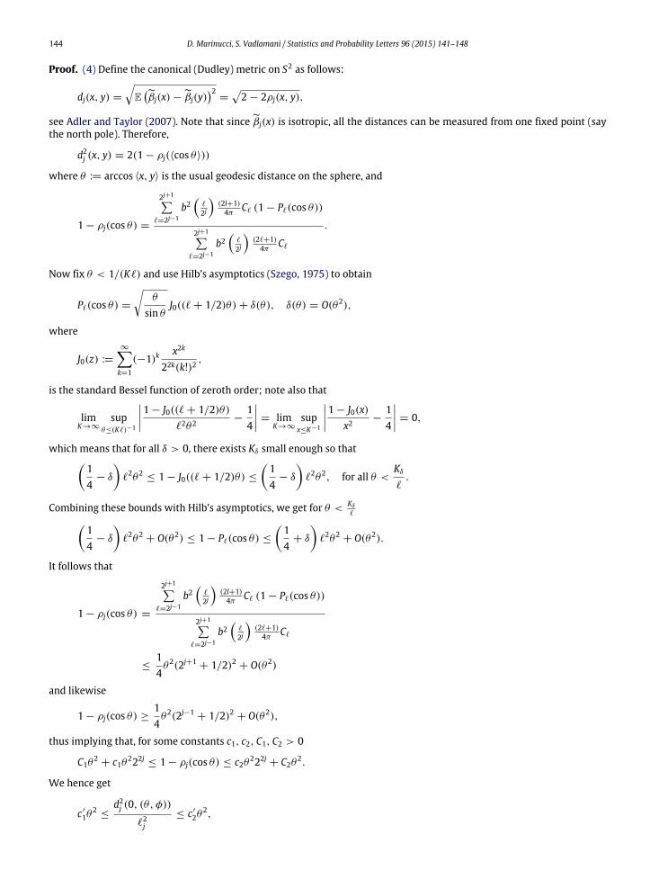
Proof. (4) Define the canonical (Dudley) metric on S2 as follows:

dj(x, y) =

Eβj(x) −βj(y)

2=2 − 2ρj(x, y),

see Adler and Taylor (2007). Note that sinceβj(x) is isotropic, all the distances can be measured from one fixed point (saythe north pole). Therefore,

d2j (x, y) = 2(1 − ρj(⟨cos θ⟩))

where θ := arccos ⟨x, y⟩ is the usual geodesic distance on the sphere, and

1 − ρj(cos θ) =

2j+1ℓ=2j−1

b2

ℓ

2j

(2l+1)4π Cℓ (1 − Pℓ(cos θ))

2j+1ℓ=2j−1

b2

ℓ

2j

(2ℓ+1)

4π Cℓ

.

Now fix θ < 1/(Kℓ) and use Hilb’s asymptotics (Szego, 1975) to obtain

Pℓ(cos θ) =

θ

sin θJ0((ℓ + 1/2)θ) + δ(θ), δ(θ) = O(θ2),

where

J0(z) :=

∞k=1

(−1)kx2k

22k(k!)2,

is the standard Bessel function of zeroth order; note also that

limK→∞

supθ≤(Kℓ)−1

1 − J0((ℓ + 1/2)θ)

ℓ2θ2−

14

= limK→∞

supx≤K−1

1 − J0(x)x2

−14

= 0,

which means that for all δ > 0, there exists Kδ small enough so that14

− δ

ℓ2θ2

≤ 1 − J0((ℓ + 1/2)θ) ≤

14

− δ

ℓ2θ2, for all θ <

Kδ

ℓ.

Combining these bounds with Hilb’s asymptotics, we get for θ <Kδ

ℓ14

− δ

ℓ2θ2

+ O(θ2) ≤ 1 − Pℓ(cos θ) ≤

14

+ δ

ℓ2θ2

+ O(θ2).

It follows that

1 − ρj(cos θ) =

2j+1ℓ=2j−1

b2

ℓ

2j

(2l+1)4π Cℓ (1 − Pℓ(cos θ))

2j+1ℓ=2j−1

b2

ℓ

2j

(2ℓ+1)

4π Cℓ

≤14θ2(2j+1

+ 1/2)2 + O(θ2)

and likewise

1 − ρj(cos θ) ≥14θ2(2j−1

+ 1/2)2 + O(θ2),

thus implying that, for some constants c1, c2, C1, C2 > 0

C1θ2+ c1θ222j

≤ 1 − ρj(cos θ) ≤ c2θ222j+ C2θ

2.

We hence get

c ′

1θ2

≤d2j (0, (θ, φ))

ℓ2j

≤ c ′

2θ2,

D. Marinucci, S. Vadlamani / Statistics and Probability Letters 96 (2015) 141–148 145

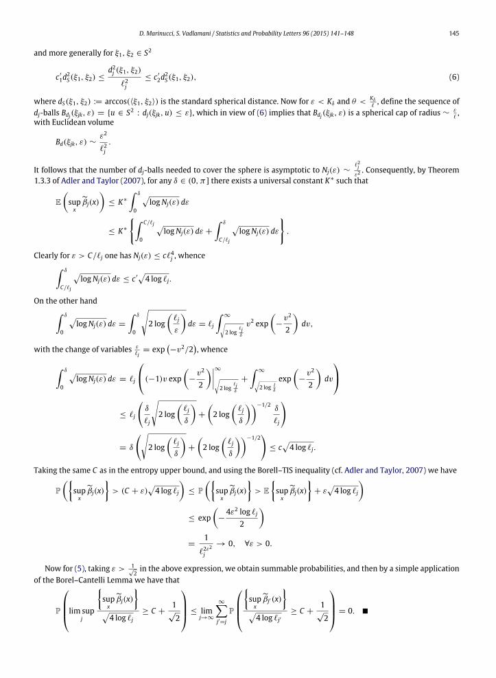
and more generally for ξ1, ξ2 ∈ S2

c ′

1d2S(ξ1, ξ2) ≤

d2j (ξ1, ξ2)

ℓ2j

≤ c ′

2d2S(ξ1, ξ2), (6)

where dS(ξ1, ξ2) := arccos(⟨ξ1, ξ2⟩) is the standard spherical distance. Now for ε < Kδ and θ <Kδ

ℓ, define the sequence of

dj-balls Bdj(ξjk, ε) = u ∈ S2 : dj(ξjk, u) ≤ ε, which in view of (6) implies that Bdj(ξjk, ε) is a spherical cap of radius ∼εℓ,

with Euclidean volume

Bd(ξjk, ε) ∼ε2

ℓ2j.

It follows that the number of dj-balls needed to cover the sphere is asymptotic to Nj(ε) ∼ℓ2jε2. Consequently, by Theorem

1.3.3 of Adler and Taylor (2007), for any δ ∈ (0, π] there exists a universal constant K ∗ such that

Esupxβj(x)

≤ K ∗

δ

0

logNj(ε) dε

≤ K ∗

C/ℓj

0

logNj(ε) dε +

δ

C/ℓj

logNj(ε) dε

.

Clearly for ε > C/ℓj one has Nj(ε) ≤ cℓ4j , whence δ

C/ℓj

logNj(ε) dε ≤ c ′

4 log ℓj.

On the other hand δ

0

logNj(ε) dε =

δ

0

2 log

ℓj

ε

dε = ℓj

∞2 log

ℓjδ

v2 exp

−v2

2

dv,

with the change of variables εℓj

= exp−v2/2

, whence

δ

0

logNj(ε) dε = ℓj

(−1)v exp

−v2

2

∞2 log

ℓjδ

+

∞2 log l

δ

exp

−v2

2

dv

≤ ℓj

δ

ℓj

2 log

ℓj

δ

+

2 log

ℓj

δ

−1/2δ

ℓj

= δ

2 log

ℓj

δ

+

2 log

ℓj

δ

−1/2

≤ c4 log ℓj.

Taking the same C as in the entropy upper bound, and using the Borell–TIS inequality (cf. Adler and Taylor, 2007) we have

P

supxβj(x)

> (C + ε)

4 log ℓj

≤ P

supxβj(x)

> E

supxβj(x)

+ ε

4 log ℓj

≤ exp

−

4ε2 log ℓj

2

=

1

ℓ2ε2j

→ 0, ∀ε > 0.

Now for (5), taking ε > 1√2in the above expression, we obtain summable probabilities, and then by a simple application

of the Borel–Cantelli Lemma we have that

P

lim supj

supxβj(x)

4 log ℓj

≥ C +1

√2

≤ limj→∞

∞j′=j

P

supxβj′(x)

4 log ℓj′

≥ C +1

√2

= 0.

146 D. Marinucci, S. Vadlamani / Statistics and Probability Letters 96 (2015) 141–148

3. Discretization and lower bounds

As explained in the Introduction, this section is devoted to the proofs for the lower bounds that follow.

Proposition 3. We have

lim infj

E

supx∈S2

βj(x)

4 log ℓj

≥ 1 (7)

and

P

lim infj

supx∈S2

βj(x)

4 log ℓj

≥ 1

= 1. (8)

Proof. We start showing that, for all δ > 0,

limj

P

supx∈S2

βj

4 log ℓj

> 1 − δ

= 1. (9)

Note first that supβj ≥ supkβj,k, where βj,k is any discrete sample taken fromβj. Now, let us choose a grid of points such

that the distance between them is at least 2−j(1−δ), for some δ > 0—e.g., a 2−j(1−δ)-net, see Baldi et al. (2009b). Note thatthe vectors βj,· andβj,· both have cardinality of order 22j(1−δ). By using the correlation inequality given in Lemma 10.8 ofMarinucci and Peccati (2011), we have

Eβj,kβj,k′ ≤CM

(1 + 2jδ)M,

where M ∈ N can be chosen arbitrarily large. The idea of the proof is to approximate these subsampled coefficients bymeans of a triangular array of Gaussian i.i.d. random variables, sayβj,k. More precisely, let Σj be the covariance matrix ofthe Gaussian vectorβj,·; then defineβj,· = Σ

−1/2j

βj,·, which is clearly a vector of i.i.d. Gaussian variables, and let λj,max andλj,min be the largest and the smallest eigenvalue of the matrix Σj. Then

λj,max, λj,min = 1 + O(εj),

for a deterministic sequenceεjwhich goes to zero faster than any polynomial (nearly exponentially). Indeed

λj,max = supx

x′Σjx = supx

x′Σj − I + I

x = sup

xx′Σj − I

x + 1

≤ ℓ4(1−δ)j

CM

1 + 2jδM+ 1,

where the bound follows crudely from the cardinality of the off-diagonal terms in the matrix. Similarly,

λj,min = infxx′Σjx = inf

xx′Σj − I + I

x

= infxx′Σj − I

x + 1 ≥ 1 − sup |x′

Σj − I

x|

≥ 1 − ℓ4j

CM

1 + ℓδMj

.

As a consequence, writing ∥ · ∥2 for the Euclidean inner product in the appropriate dimension we have

Esupk

|βj,k −βj,k|

≤

E∥βj,· −βj,·∥

22

=

E∥(I − Σ−1/2)βj,·∥

22 ≤ |1 − λ−1/2

max |

E∥βj,·∥

22

≤ ℓ4(1−δ)j

CM

1 + ℓδMj

· ℓ2j = ℓ

2+4(1−δ)j

CM

1 + ℓδMj

= O(ℓ6−δMj ).

D. Marinucci, S. Vadlamani / Statistics and Probability Letters 96 (2015) 141–148 147

We can now exploit a classical result by Berman (1962) to conclude that

P

supk

βj,k4 log ℓj

− 1

> ε

→ 0,

as j → ∞, for all ε > 0. Thus (9) is established; (7) follows immediately, given that δ is arbitrary. To establish (8), we useagain the Borel–Cantelli Lemma, so that we need to prove that, for all ε > 0

j

P

supx∈S2

βj

4 log ℓj

< 1 − ε

< ∞.

Clearly

P

supx∈S2

βj

4 log ℓj

< 1 − ε

≤ P

supk

βj,k4 log ℓj

< 1 − ε

, for all j, (10)

whence it suffices to prove that

j

P

supk

βj,k4 log ℓj

< 1 − ε

< ∞.

Now

P

supk

βj,k4 log ℓj

< 1 − ε

= P

supk

βj,k −βj,k +βj,k

4 log ℓj

< 1 − ε

≤ P

supk

βj,k − supk

βj,k −βj,k

4 log ℓj

< 1 − ε

≤ P

supk

βj,k − supk

βj,k −βj,k

4 log ℓj< 1 − ε

= P

supk

βj,k4 log ℓj

< 1 − ε +

supk

βj,k −βj,k

4 log ℓj

≤ P

supk

βj,k4 log ℓj

< 1 −ε

2

+ P

supk

βj,k −βj,k

4 log ℓj>

ε

2

≤ P

supk

βj,k4 log ℓj

< 1 −ε

2

+ O(ℓ6−δMj ).

The second term above is clearly summable by simply taking M large enough. To check summability of the first term wewrite

P

supk

βj,k4 log ℓj

< 1 −ε

2

=

k

P

βj,k4 log ℓj

< 1 −ε

2

=

1 − P

βj,1 >1 −

ε

2

4 log ℓj

ℓ2(1−δ)j

148 D. Marinucci, S. Vadlamani / Statistics and Probability Letters 96 (2015) 141–148

≤

1 −1

1 −ε2

4 log ℓj

1 −

11 −

ε2

4 log ℓj

·

1

ℓ2(1− ε

2 )2

j

ℓ2(1−δ)j

≤

1 −1

21 −

ε2

4 log ℓj

·1

ℓ2(1− ε

2 )2

j

ℓ2(1−δ)j

=

1 −1

21 −

ε2

4 log ℓj

·1

ℓ2(1− ε

2 )2

j

2(1− ε2 )

√4 log ℓjℓ

2(1− ε2 )

2

jℓ2(1−δ)j

2(1− ε2 )

√4 log ℓjℓ

2(1− ε2 )

2

j

≤ exp

−ℓ2(1−δ)−(1− ε

2 )2

j

21 −

ε2

4 log ℓj

≤ exp

−ℓ2[(1−δ)−(1− ε

2 )]j

21 −

ε2

4 log ℓj

≤ exp

−ℓ2[ ε

2 −δ]j

21 −

ε2

4 log ℓj

where we have used Mill’s inequality for standard Gaussian variables, P Z > z ≥

z1+z2

φ(z). This is summable wheneverε > 2δ, which can easily be obtained by choosing such a delta in Eq. (10).

Acknowledgement

Research supported by the ERC Grant no. 277742 Pascal, ‘‘Probabilistic and Statistical Techniques for CosmologicalApplications’’.

References

Adler, R.J., Taylor, J.E., 2007. Random Fields and Geometry. Springer.Azaïs, J.-M., Wschebor, M., 2009. Level Sets and Extrema of Random Processes and Fields. John Wiley & Sons, Inc., Hoboken, NJ.Baldi, P., Kerkyacharian, G., Marinucci, D., Picard, D., 2009a. Asymptotics for spherical needlets. Ann. Statist. 37 (3), 1150–1171.Baldi, P., Kerkyacharian, G., Marinucci, D., Picard, D., 2009b. Subsampling needlet coefficients on the sphere. Bernoulli 15, 438–463.Bennett, C.L., et al. 2012. Nine-year WMAP observations: final maps and results. arXiv:1212.5225.Berman, S., 1962. A law of large numbers for the maximum in a stationary Gaussian sequence. Ann. Math. Stat. 33 (1), 93–97.Cammarota, V., Marinucci, D., 2014. On the limiting behaviour of needlets polyspectra. Ann. Inst. H. Poincaré, in press, arXiv:1307.4691.Cheng, D., Schwartzman, A., 2013. Distribution of the height of local maxima of Gaussian random fields. arXiv:1307.5863.Cheng, D., Xiao, Y., 2012. The mean Euler characteristic and excursion probability of Gaussian random fields with stationary increments. arXiv:1211.6693.Marinucci, D., Peccati, G., 2011. Random Fields on the Sphere. Representation, Limit Theorem and Cosmological Applications. Cambridge University Press.Marinucci, D., Peccati, G., 2012. Mean square continuity on homogeneous spaces of compact groups. arXiv:1210.7676.Marinucci, D., Vadlamani, S., 2013. High-frequency asymptotics for Lipschitz–Killing curvatures of excursion sets on the sphere. arXiv:1303.2456.Narcowich, F.J., Petrushev, P., Ward, J.D., 2006a. Localized tight frames on spheres. SIAM J. Math. Anal. 38, 574–594.Pietrobon, D., Amblard, A., Balbi, A., Cabella, P., Cooray, A., Marinucci, D., 2008. Needlet detection of features in WMAP CMB sky and the impact on

anisotropies and hemispherical asymmetries. Phys. Rev. D 78, 103504.Stein, E.M., Weiss, G., 1971. Introduction to Fourier Analysis on Euclidean Spaces. Princeton University Press.Szego, G., 1975. Orthogonal Polynomials, fourth ed. In: Colloquium Publications, vol. XXIII. American Mathematical Society.Zelditch, S., 2009. Real and complex zeros of Riemannian random waves. Contemp. Math. 484, 321–342.